Embed Size (px)
Citation preview

A Better Way to DesignCommunication Protocols
Friedger Muffke
A thesis submitted to the University of Bristol in accordance with the requirements of thedegree of Doctor of Philosophy in the Faculty of Engineering, Department of Computer
Science
May 2004
Word Count: 38.586


Abstract
In this thesis a framework for the design of communication protocols is presented. It providesa theoretical foundation for an existing design method used in industry. The framework sup-ports the specification of protocols as well as the generation of protocol interfaces. For thespecification an appropriate formal design language is defined based on dataflow algebras. Thelanguage contains operators for conditional choice, hierarchical modelling and the specifica-tion of pipelines. For a protocol specification the framework provides decomposition rules thatproduce an interface for each component of the system for which the protocol has been defined.These rules formally relate dataflow-algebraic models with process-algebraic ones. Thus, theframework provides an intuitive and general as well as formally defined design method forcommunication protocols. As a case study the PI-bus protocol has been modelled using thisframework.


Acknowledgements
Firstly, I would like to thank my supervisor, Kerstin Eder. She supported and encouraged meto explore both theoretical and practical aspects of the broader research field of this thesis andprovided helpful feedback to tie up loose ends.
I am grateful for productive discussions with Greg Jablonwsky, James Edwards and GeraldLuettgen. Furthermore, I want to thank Kerstin Eder, Henk Muller, Jean and John, and Adinafor proof reading all or parts of this thesis. Their constructive feedback has helped to improvethis work.
I was supported during my PhD studies by a scholarship of the Department of ComputerScience and the EPSRC (GR/M 93758).


Declaration
I declare that the work in this dissertation was carried out in accordance with the Regulationsof the University of Bristol. The work is original except where indicated by special referencein the text and no part of the dissertation has been submitted for any other degree.
Any views expressed in the dissertation are those of the author and in no way representthose of the University of Bristol. The dissertation has not been presented to any other Univer-sity for examination either in the United Kingdom or overseas.
Signed: . . . . . . . . . . . . . . . . . . . . . . . . . . . . . . . . . . . . . . . . . . . . . .
Date: . . . . . . . . . . . . . . . . . . . . . . .


Contents
1 Introduction 31.1 Motivation. . . . . . . . . . . . . . . . . . . . . . . . . . . . . . . . . . . . . 31.2 The Challenge of Protocol Verification . .. . . . . . . . . . . . . . . . . . . . 51.3 Sketch of Solution .. . . . . . . . . . . . . . . . . . . . . . . . . . . . . . . . 51.4 Roadmap of the Thesis. . . . . . . . . . . . . . . . . . . . . . . . . . . . . . 7
2 Protocols and Specification Languages 92.1 Protocols . . . . . . . . . . . . . . . . . . . . . . . . . . . . . . . . . . . . . 9
2.1.1 Protocol Specification. . . . . . . . . . . . . . . . . . . . . . . . . . 102.1.2 Protocol Interfaces . .. . . . . . . . . . . . . . . . . . . . . . . . . . 11
2.2 Approaches to Formal Modelling. . . . . . . . . . . . . . . . . . . . . . . . . 122.2.1 Dataflow-oriented Descriptions .. . . . . . . . . . . . . . . . . . . . 132.2.2 Process-oriented Descriptions . .. . . . . . . . . . . . . . . . . . . . 13
2.3 Protocol Specification and Description Languages .. . . . . . . . . . . . . . . 142.3.1 Estelle . . .. . . . . . . . . . . . . . . . . . . . . . . . . . . . . . . . 152.3.2 Lotos . . .. . . . . . . . . . . . . . . . . . . . . . . . . . . . . . . . 162.3.3 SDL. . . . . . . . . . . . . . . . . . . . . . . . . . . . . . . . . . . . 162.3.4 Esterel . .. . . . . . . . . . . . . . . . . . . . . . . . . . . . . . . . 172.3.5 Interface Description Languages .. . . . . . . . . . . . . . . . . . . . 18
2.4 Process Algebras .. . . . . . . . . . . . . . . . . . . . . . . . . . . . . . . . 182.4.1 Syntax . .. . . . . . . . . . . . . . . . . . . . . . . . . . . . . . . . 192.4.2 Semantics .. . . . . . . . . . . . . . . . . . . . . . . . . . . . . . . . 202.4.3 Extensions to Process Algebras .. . . . . . . . . . . . . . . . . . . . 20
2.5 Dataflow Algebras . . . . . . . . . . . . . . . . . . . . . . . . . . . . . . . . 222.5.1 Introduction. . . . . . . . . . . . . . . . . . . . . . . . . . . . . . . . 222.5.2 Syntactic Modelling Level. . . . . . . . . . . . . . . . . . . . . . . . 242.5.3 Semantics .. . . . . . . . . . . . . . . . . . . . . . . . . . . . . . . . 262.5.4 Relation to Process Algebras . . .. . . . . . . . . . . . . . . . . . . . 27
2.6 SystemCSV . . . . . . . . . . . . . . . . . . . . . . . . . . . . . . . . . . . . 29
3 Conditional Choice based on Previous Behaviour 313.1 Introduction . . . . . . . . . . . . . . . . . . . . . . . . . . . . . . . . . . . . 313.2 Logic with Past Operator . . .. . . . . . . . . . . . . . . . . . . . . . . . . . 32
3.2.1 Semantics .. . . . . . . . . . . . . . . . . . . . . . . . . . . . . . . . 333.2.2 Logic with Past and Clock Signals. . . . . . . . . . . . . . . . . . . . 35
vii

viii CONTENTS
3.3 Conditional Choice in Dataflow Algebra . .. . . . . . . . . . . . . . . . . . . 353.3.1 Reducing Formulae. . . . . . . . . . . . . . . . . . . . . . . . . . . . 373.3.2 Semantics of the Conditional Choice. . . . . . . . . . . . . . . . . . . 413.3.3 Properties . . .. . . . . . . . . . . . . . . . . . . . . . . . . . . . . . 42
3.4 Conditional Choice in Process Algebra . . .. . . . . . . . . . . . . . . . . . . 453.4.1 Related Work .. . . . . . . . . . . . . . . . . . . . . . . . . . . . . . 453.4.2 Compositional Semantics. . . . . . . . . . . . . . . . . . . . . . . . 463.4.3 Property Processes. . . . . . . . . . . . . . . . . . . . . . . . . . . . 493.4.4 One-way Communication. . . . . . . . . . . . . . . . . . . . . . . . 503.4.5 Building Property Processes. . . . . . . . . . . . . . . . . . . . . . . 51
3.5 Summary . .. . . . . . . . . . . . . . . . . . . . . . . . . . . . . . . . . . . 54
4 Hierarchical Modelling 574.1 Introduction .. . . . . . . . . . . . . . . . . . . . . . . . . . . . . . . . . . . 574.2 Related Work . . . . . . . . . . . . . . . . . . . . . . . . . . . . . . . . . . . 594.3 Action Refinement for Protocol Design . .. . . . . . . . . . . . . . . . . . . 604.4 Semantics . .. . . . . . . . . . . . . . . . . . . . . . . . . . . . . . . . . . . 62
4.4.1 Extensions to the Operational Semantics. . . . . . . . . . . . . . . . . 634.4.2 Hiding Implementation Details . . .. . . . . . . . . . . . . . . . . . . 644.4.3 Synchronisation . . . . . . . . . . . . . . . . . . . . . . . . . . . . . 65
4.5 Difference between Dataflow Algebra and Process Algebra . . .. . . . . . . . 664.6 Summary . .. . . . . . . . . . . . . . . . . . . . . . . . . . . . . . . . . . . 67
5 Framework 695.1 Communication Items .. . . . . . . . . . . . . . . . . . . . . . . . . . . . . . 70
5.1.1 Definition . . .. . . . . . . . . . . . . . . . . . . . . . . . . . . . . . 705.1.2 Semantics . . .. . . . . . . . . . . . . . . . . . . . . . . . . . . . . . 72
5.2 Specification Process .. . . . . . . . . . . . . . . . . . . . . . . . . . . . . . 735.2.1 Hierarchical Development. . . . . . . . . . . . . . . . . . . . . . . . 745.2.2 Top-Level Specification .. . . . . . . . . . . . . . . . . . . . . . . . 755.2.3 Pipelines . . .. . . . . . . . . . . . . . . . . . . . . . . . . . . . . . 755.2.4 Comments . .. . . . . . . . . . . . . . . . . . . . . . . . . . . . . . 80
5.3 Interface Generation .. . . . . . . . . . . . . . . . . . . . . . . . . . . . . . 825.3.1 Decomposition Operators. . . . . . . . . . . . . . . . . . . . . . . . 835.3.2 Structural Changes. . . . . . . . . . . . . . . . . . . . . . . . . . . . 85
5.4 Implementation of Interfaces . . .. . . . . . . . . . . . . . . . . . . . . . . . 885.4.1 Dealing with Non-Relevant Items .. . . . . . . . . . . . . . . . . . . 885.4.2 Satisfying Constraints . .. . . . . . . . . . . . . . . . . . . . . . . . 89
5.5 Models with Global Clock Signals. . . . . . . . . . . . . . . . . . . . . . . . 905.5.1 Specifying Clock Cycles .. . . . . . . . . . . . . . . . . . . . . . . . 915.5.2 Timing Information of Clock Cycles. . . . . . . . . . . . . . . . . . . 925.5.3 Implementing Synchronisation . . .. . . . . . . . . . . . . . . . . . . 93
5.6 Summary . .. . . . . . . . . . . . . . . . . . . . . . . . . . . . . . . . . . . 93

CONTENTS ix
6 Case Study: PI-Bus 956.1 Protocol Specification. . . . . . . . . . . . . . . . . . . . . . . . . . . . . . . 96
6.1.1 Transaction. . . . . . . . . . . . . . . . . . . . . . . . . . . . . . . . 966.1.2 Phase-Level Modelling. . . . . . . . . . . . . . . . . . . . . . . . . . 976.1.3 Signal-Level Implementation . . .. . . . . . . . . . . . . . . . . . . . 986.1.4 Topology .. . . . . . . . . . . . . . . . . . . . . . . . . . . . . . . . 996.1.5 Top-Level Specification. . . . . . . . . . . . . . . . . . . . . . . . . 101
6.2 Interface Generation. . . . . . . . . . . . . . . . . . . . . . . . . . . . . . . 1026.2.1 Master Interface . . .. . . . . . . . . . . . . . . . . . . . . . . . . . 1036.2.2 Slave Interface. . . . . . . . . . . . . . . . . . . . . . . . . . . . . . 1046.2.3 Controller Interface . .. . . . . . . . . . . . . . . . . . . . . . . . . . 1066.2.4 Composition . . . . . . . . . . . . . . . . . . . . . . . . . . . . . . . 108
6.3 Clock . . . . . . . . . . . . . . . . . . . . . . . . . . . . . . . . . . . . . . . 1086.3.1 Specification . . . . . . . . . . . . . . . . . . . . . . . . . . . . . . . 1086.3.2 Implementation. . . . . . . . . . . . . . . . . . . . . . . . . . . . . . 109
6.4 Conclusions. . . . . . . . . . . . . . . . . . . . . . . . . . . . . . . . . . . . 110
7 Conclusions 1117.1 Summary . . . . . . . . . . . . . . . . . . . . . . . . . . . . . . . . . . . . . 111
7.1.1 Comparison with Similar Approaches . . .. . . . . . . . . . . . . . . 1137.1.2 Hierarchical Modelling. . . . . . . . . . . . . . . . . . . . . . . . . . 1147.1.3 Time . . .. . . . . . . . . . . . . . . . . . . . . . . . . . . . . . . . 115
7.2 Future Work. . . . . . . . . . . . . . . . . . . . . . . . . . . . . . . . . . . . 1157.2.1 Tool Support . . . . . . . . . . . . . . . . . . . . . . . . . . . . . . . 1157.2.2 Semantics of Dataflow Algebra .. . . . . . . . . . . . . . . . . . . . 1167.2.3 Low-level Communication. . . . . . . . . . . . . . . . . . . . . . . . 117
7.3 Further Application Areas . .. . . . . . . . . . . . . . . . . . . . . . . . . . 1177.3.1 Protocol Bridges . . .. . . . . . . . . . . . . . . . . . . . . . . . . . 1177.3.2 Performance Analysis. . . . . . . . . . . . . . . . . . . . . . . . . . 118
A VHDL-like Specification Language 119
Bibliography 129


List of Figures
3.1 Choice Dependent onϕ . . . . . . . . . . . . . . . . . . . . . . . . . . . . . . 313.2 Past Operators . . .. . . . . . . . . . . . . . . . . . . . . . . . . . . . . . . . 333.3 Topology ofSys . . . . . . . . . . . . . . . . . . . . . . . . . . . . . . . . . 443.4 Resolving Conditional Choice. . . . . . . . . . . . . . . . . . . . . . . . . . 49
4.1 Hierarchy: One-World View and Multi-World View. . . . . . . . . . . . . . . 584.2 Hierarchical Refinement . . .. . . . . . . . . . . . . . . . . . . . . . . . . . 61
5.1 Three-stage Pipeline. . . . . . . . . . . . . . . . . . . . . . . . . . . . . . . 805.2 Decomposition of Example . .. . . . . . . . . . . . . . . . . . . . . . . . . . 865.3 Splitting Parallel Composition. . . . . . . . . . . . . . . . . . . . . . . . . . 87
6.1 Routing Plan for High-Level Signals . . .. . . . . . . . . . . . . . . . . . . . 99
xi


List of Tables
3.1 Definition oftail andhead for Dataflow Algebra Sequences .. . . . . . . . . 343.2 Defintion of|=r . . . . . . . . . . . . . . . . . . . . . . . . . . . . . . . . . . 353.3 Definition of|=r for Clocked Past Operators. . . . . . . . . . . . . . . . . . . 363.4 Relevant Actions for Basic Present Properties . . .. . . . . . . . . . . . . . . 53
5.1 Precedence Hierarchy. . . . . . . . . . . . . . . . . . . . . . . . . . . . . . . 715.2 Deduction Rules for Pipeline Operators .. . . . . . . . . . . . . . . . . . . . 785.3 Definition of Optimisation Functionopt . . . . . . . . . . . . . . . . . . . . . 895.4 Decomposition of Clock Signals. . . . . . . . . . . . . . . . . . . . . . . . . 92
6.1 Topology of Read Transactions. . . . . . . . . . . . . . . . . . . . . . . . . . 100
1


Chapter 1
Introduction
1.1 Motivation
A communication protocol is defined as a set of conventions governing the format and control
of interaction among communicating functional units, e.g. for systems-on-chip these units are
the processor unit, on-chip memory, floating point arithmetic unit and similar components. The
set of conventions specifies the behaviour of the protocol and may contain certain constraints
about the environment the protocol may be applied in.
Generally speaking, specifications are used to define a framework within which design-
ers have to implement a system. Specifications have to be intuitive, easy to understand and
expressive enough to exclude ambiguities. On one hand specifications can be made in plain
English using pictures and diagrams as well to make the meaning of the specification easy to
understand, however ambiguities can not be excluded as text and diagrams can be interpreted
differently. On the other hand, formal specifications do not leave space for ambiguities, they
can be used to automate design as the semantics of the specification language can be supported
by tools. However, they are more difficult to write and to understand for designers because less
formal methods used to be more common.
Nevertheless, formal specifications become increasingly important as the complexity of the
designed systems grows. With the complexity of the system the time needed to verify existing
system models increases exponentially. In industry the gap between the size of system models
that are feasible to be modelled and manufactured and those that can be verified is growing
3

1.1 Motivation
rapidly, so-called verification gap [42].
The verification task consists of ensuring that the built system works as expected, there
is no mentioning of the methods how this is ensured and what level of confidence has been
achieved. In industry, the most common way of verifying a system is by simulation. In theo-
retical computer science, verification is defined as formally establishing a relationship between
different models. One model precisely specifies the requirements of the system. The other
more detailed model is verified against these requirements. Using formal methods, theorems
in mathematical sense are established to show whether the model satisfies the requirements or
not.
The drawback of formal verification is that the verification result is only as good as the
formal specification. Due to their formal nature, formal specifications can contain errors more
easily than verification tasks using simulation, debugging and human intuition. Therefore, it is
necessary to define methods and develop tools to increase the confidence in and reduce errors
of formal specifications. Otherwise, the specification has to be verified in the same way as the
implemented model.
The most important condition to successfully complete verification is to know what exactly
the verification task needs to achieve. This seems to be trivial. However, in practice formal
methods are often not applied due to a lack of awareness for the verification goal. In contrast
to simulation where certain behaviours of the system are tested, formal verification needs an
abstract understanding of the properties of the system.
There are several different approaches how to model communication protocols and there
are several tools (e.g. SPIN [28], FDR [26], VIS [54]) available that apply formal methods like
model checking, refinement checking or theorem proving to formally show the correctness of
the implementation, i.e. that the implementation satisfies the specification. Depending on the
methods used, the result can be obtained automatically or interactively.
However, until now there does not exist any commercial tool that formally verifies the cor-
rectness of protocols. Existing design methods do not provide a suitable framework for design-
ing communication protocols that are formal and general. In this thesis, existing approaches
are discussed and from there a modelling method is developed that ensures the correctness of
a protocol implementation by construction. A more detailed outline is given at the end of this
chapter.
4

1.2 The Challenge of Protocol Verification
1.2 The Challenge of Protocol Verification
The task of protocol verification consists of ensuring that the design of the protocol satisfies the
expectations and specifications given to the designer. One has to clearly distinguish between
the specifications a protocol designer publishes and the designer’s intention during the design
process because both often differ from each other, in practice e.g. due to complexity of the
problem or negligence during the design.
The implementation of communication protocols has to deal with difficulties arising from
the fact that the concerted behaviour of several components should result in the correct com-
munication between these components.
In [58] it has been shown for a preliminary specification of the PI-bus communication pro-
tocol that even with a correct specification the implemented system can be erroneous if the
specification is not stringent enough. In this case, some components of the system can imple-
ment the same specification differently and the whole system might fail to work at all. Weak
specifications cause problems in particular in communication protocols where communication
behaviour is specified independently of the remaining, not communication-related behaviour
of the components.
However, if the specification is too rigorous it fails to supply a framework for the designer.
It can be used as an implementation without any changes and the verification task is transferred
from the implementation to the specification. Hence, a method is necessary that allows to
specify systems without giving to much details and still exclude ambiguities.
The correct and verified design of protocols is still an unsolved problem. The problem
becomes apparent when analysing documentations of specifications and standards. They are
often informal and not easy to understand. Ambiguities cannot be excluded, especially when
it comes to implementation details. Furthermore, practical problems such as uniting different
manufacturers’ own designs in a standard have to be overcome.
1.3 Sketch of Solution
The classical description of a communication protocol takes a process-oriented view that de-
scribes the behaviour of each single component that participates at the communication. Process
5

1.3 Sketch of Solution
algebras1 have been developed to model such systems, i.e. concurrent communicating systems.
Their theory has been studied in great detail and various extensions have been developed. How-
ever, there is still work necessary to transfer the theoretical knowledge into applications. Thus,
the motivation was to investigate the applicability of process algebras for modelling modern
system-on-chip communication protocols. It became apparent that the presented work can be
applied in a more general context than this type of protocols. However, improving systems-on-
chip protocol design has been the original motivation.
The process-oriented view is most useful for implementation purposes. However, this ap-
proach makes it difficult to understand the overall behaviour of the protocol [27]. To reuse and
extend these protocol components becomes even more difficult as they are often specifically
designed for a certain environment.
A more appropriate design method would take a system-wide view of the protocol that
focuses on the global functioning of the communicating system. The main advantage of the
system-wide view is that the protocol specification considers the dataflow controlled by the
protocol instead of the behaviour of system components, which might or might not result in the
correct dataflow when combined with other components. Furthermore, from a global descrip-
tion the behaviour of the system components can be derived in a refinement-based approach
such that extensions and changes in the protocol will be reflected in the derived behaviour of
the components. This approach is formalised in dataflow algebras2.
For the design of communication protocols both methods should be combined because
communication protocols exhibits two different aspect of the system that uses the protocol:
Firstly, what kind of messages are communicated and when. Secondly, what each component
has to do in order to be compliant to the protocol. Dataflow algebras give a system-wide view
of all valid traces of a system and force the designer to concentrate on the properties and the
purpose of the protocol instead of focusing on the components of the system prematurely. In
contrast, process algebras naturally support composed models and include a way to abstract
from certain behaviour.
The combination and connection of the two formalisms allows both to globally specify the
protocol and to derive behaviours for system components. As the two formalisms are based on
1For references see Section 2.4.2For references see Section 2.5.
6

1.4 Roadmap of the Thesis
different semantics, a translation between them or a common semantics has to be found.
In order to handle the complexity of a system-wide specification, it is standard practice to
introduce protocol layers and describe the protocol parts in an hierarchical manner. Therefore,
the formalism should support hierarchical modelling.
1.4 Roadmap of the Thesis
The remaining chapters of this thesis are structured as follows. In the next chapter the ele-
ments of protocol design are presented. First, communication protocols are classified by their
properties. Second, a description of existing design methods and design languages for proto-
cols follows. The main focus here is on formal approaches using dataflow algebra and process
algebra.
In Chapter 3 and 4 two additional modelling features are introduced to dataflow algebra and
process algebra. These are conditional choice based on previous behaviour and hierarchical
modelling. Both features can be naturally embedded into the formalisms and are necessary for
a convenient design method for protocols.
The new design method for communication protocols is described in its entirety in Chap-
ter 5. It consists of a detailed explanation of the different design steps and how the interfaces for
the system components are derived from the global specification. The modelling of pipelines
is described as well as the effects of global clock signals which are often present in systems-
on-chip.
In Chapter 6 the method is exercised on a case study based on the open source protocol
of the PI-bus. This is a high performance bus protocol with a two-stage pipeline. It is also
outlined how the modelling of a three-stage pipeline would differ.
The last chapter concludes the thesis comparing the framework with existing methods. Its
usability in existing design flows and possible tool support is discussed. Finally prospects on
further research topics in this area are given.
7


Chapter 2
Protocols and Specification Languages
2.1 Protocols
Communication protocols describe the synchronous or asynchronous interaction between in-
dependent processes, i.e. functional units of a system, with the purpose of transferring informa-
tion between them. They rely on a usually fixed topology of the system defined by connections
between the processes. These connections are called channels.
Uni-directional channels describe the connection between a sending process that transfers
information just in one direction and possibly several receiving processes. Multi-directional
channels are used to send and receive information in any direction. If necessary, this type of
channel can be modelled as a collection of uni-directional channels.
A connection that can be used by more than one sending processes is called a bus or bus
channel. To ensure that the bus is not used by two sending processes at the same time a control
mechanism has to be introduced. It can consist of rigid timing constraints (scheduling) or a
separate control process that grants access to the bus.
Depending on the communication channel one distinguishes between synchronous and
asynchronous communication.
Synchronous communication imposes restrictions on participating components regarding
the time when communication may occur. Components are blocked until all participating com-
ponents are ready to perform the communication. This way of communication is, for example,
realised when rendez-vous channels are used.
9

2.1 Protocols
Asynchronous communication does not impose any restriction on the behaviour of the pro-
cesses. As a consequence the communicating components in general do not have any knowl-
edge about whether a message was received and how long the communication took.
Asynchronous communication is a super category of synchronous communication. Syn-
chronous communication can be modelled on the basis of asynchronous communication by
confirming the receipt of each message using so called handshake protocols.
Most protocols whether based on asynchronous or synchronous communication distinguish
between control channels and data channels. Control channels are only used to transmit infor-
mation about the state of the processes and of the data channels. The information itself is
transmitted via data channels and does not influence the behaviour of the protocol. However,
some protocols, e.g. the alternating bit protocol [25] or HTTP [40], encode control information
within the transmitted data in order to minimize the necessary bandwidth.
Depending on the number of participating processes one differentiates several classes of
protocols. For example, multi-cast protocols, like ad-hoc network protocols [41], allow to
transmit data to several receivers at the same time. In contrast, one-to-one protocols only allow
communication between two single processes, like the open core protocol [62].
The way of transmitting data is also used to classify protocols. In handshake protocols the
reception of a message is always confirmed, whereas in timed protocols messages are tagged
with time stamps and the successful delivery is determined from an estimated transmission
duration.
Hardware protocols transmit information via wires and have to take into account when and
for how long the information has to be driven. An example of a hardware protocols is the
PI-bus protocol [60]. It uses a bus architecture and is the basis for many system-on-chip bus
protocols. It will be discussed in depth in Chapter 6.
2.1.1 Protocol Specification
The description of a protocol has to specify whether the communication is synchronous or
asynchronous, multi-cast or one-to-one. However, in most cases the fundamental setting is
clear from the context of the protocol’s intended use. The main part of the specification then
focuses on the description of how information is transmitted.
The complete procedure of transmitting data is called a transaction. Usually, a protocol
10

2.1 Protocols
offers several transaction types that are used for the same topology of processes. A transaction
is described by messages that are passed between processes. Each message can consist of sub-
parts called packets, atomic actions or signals which are transmitted on the lowest level of the
system.
This kind of decomposition of a transaction is used to simplify the specification process
as well as to enable the separation of different aspects of the protocol. The most abstract
description is the transaction itself (transaction level); at the lowest level the transfer of each
single information bit is described respecting the physical properties of the system.
If the protocol relies on certain properties of the channels, these have to be explicitly stated
in the description of the protocol. If necessary, an additional protocol has to be used to ensure
that these properties are satisfied. In this case so-called protocol stacks or protocol layers
are built. A well known example for a protocol layer is the web service protocol SOAP [61]
which is built on top of HTTP [40]. Even more, the internet protocol can only be used for
reliable communication channels and therefore relies on the low-level internet protocol TCP
[67], which provides the necessary reliability for unreliable channels.
In addition to the layered decomposition, a protocol can also exhibit a temporal decom-
position. This kind of decomposition divides transactions into phases, which group messages
into meaningful sections. For example, the transfer of data describes one phase, the preparation
before the actual transfer another.
Furthermore, a complete protocol specification describes also the bandwidth of the chan-
nels and the format of the data and control information. However, in this thesis the influence
of these details is not considered to play an important role and, therefore, is not studied further.
Also data manipulations and their effects, the key points in security protocols, are not relevant.
For more information on these topics the reader can refer among others to [48].
2.1.2 Protocol Interfaces
Protocols give a global view of the possible communication between processes. They do not
describe the behaviour of a process that uses the protocol. However, when it comes to the
implementation of a protocol one has to take a different viewpoint. The transactions are not the
central object of interest anymore but the focus is on the behaviour of each process. The view
changes to a process-oriented one.
11

2.2 Approaches to Formal Modelling
The protocol is part of the specification for a process in the sense that the process has
to implement an interface of the protocol in order to be compliant to the protocol. Protocol
interfaces describe the parts of the protocol that a process has to perform in order to play a
particular role in the protocol. For each role a process may have during the execution of the
protocol a separate interface has to be implemented.
If the protocol distinguishes between different roles for processes, meaning that processes
can have different tasks in the protocol, then the process is said to be compliant to a protocol
role if it implements the interface for this role.
The complement of an interface with respect to the protocol is the behaviour of the re-
maining system observed through the interface. This is the environment of the process. The
environment together with the interface is equal to the protocol itself. The environment is used
when the process is tested how it behaves using the protocol.
The interface description can be derived from the global specification of the protocol. The
interface of a specific process results from the protocol by extracting the information about
the channels to be accessed and the time of access by the process. The access points are
called ports. One distinguishes between readable and writeable ports. In this thesis reading
from a channel is denoted in a CSP-like syntax [56] by a question mark after the channel’s
name, e.g.data? for channeldata , write actions by an exclamation mark, e.g.data!. If a
channel abstracts from the immediate transmission of information and describes a higher level
of communication read and write actions are not used, instead access to these channels is just
denoted by the channel name, e.g.data .
Note that the composition of the interfaces does not represent the whole protocol as the
information about the channels is not included. Only in conjunction with a model for each
channel, it is possible to reconstruct the protocol from the interfaces.
2.2 Approaches to Formal Modelling
In the previous section it has been explained that protocols can be described from the viewpoint
of the processes or from the viewpoint of the whole system. Depending on the viewpoint,
different approaches are used to formally describe protocols. The global view of a protocol is
best represented by a language that focuses on the data flow of a system, the process-oriented
12

2.2 Approaches to Formal Modelling
view requires a language that conveniently models the behaviour of communicating concurrent
systems.
2.2.1 Dataflow-oriented Descriptions
The dataflow of a system describes how data are manipulated or transformed in the system.
The description does not contain information about when and where the data is processed, only
the processing itself is described. It is assumed that data is processed as soon as it is available;
there is no explicit notation of time.
The most common description language to represent dataflow is a dataflow diagram. It
provides a technique for specifying parallel computations at a fine-grained level, usually in
the form of two-dimensional graphs where instructions available for concurrent execution are
written alongside each other while those that must be executed in sequence are written one
under the other. Data dependencies between instructions are indicated by directed arcs.
Alternative approaches, such as dataflow algebra (see Section 2.5) use grammar-based de-
scriptions. Grammars define valid patterns of a given language, e.g. in form of regular expres-
sions. In the case of protocols, the language is the set of communicated messages and valid
patterns are the valid communication patterns.
Automatic generation of pattern recognisers from grammar-based descriptions has been ap-
plied in the area of software compilers for a long time [1]. More recently, techniques from these
experiences have been transferred to hardware synthesis. For example, grammar-based spec-
ifications have been used to generate finite state machines described in VHDL [57, 52]. The
definition of the Protocol Grammar Interface Language provides a more theoretical foundation
for automatic interface generation using push-down automata [12].
2.2.2 Process-oriented Descriptions
The process-oriented view describes a system as a processing unit or a transformational system
that takes a body of input data and transforms it into a body of output data [24]. There are two
different approaches to describe systems from this viewpoint. One focuses on the states of the
system and offers a convenient way to describe them. For example, action systems [2] take this
approach. The second approach supports the intuitive description of the behaviour of a system
13

2.3 Protocol Specification and Description Languages
like process algebras [9] or Petri nets [55] do.
When protocols are described from the viewpoint of the processes of a system the language
has to reflect that processes progress concurrently. In formal languages so called maximal par-
allelism is assumed. That means concurrent processes are not in competition for resources like
processor time or memory; there are no implicit scheduling considerations. One distinguishes
between asynchronous and synchronous concurrent languages.
Asynchronous concurrent programming languages like CSP [39], Occam [6], Ada [69] de-
scribe processes as loosely coupled independent execution units, each process can evolve at
its own pace and an arbitrary amount of time can pass between the desire and the actual com-
pletion of communication. These languages also support non-deterministic behaviour meaning
that several actions are offered for execution at the same time. As there is no control about
which process may progress first, non-determinism is naturally embedded in asynchronous
concurrent languages. [11]
Synchronous concurrent programming languages like Esterel [10], Lustre [34], Signal [8]
or Statecharts [35] are used to model processes that react instantaneously to their input. The
processes communicate by broadcasting information instantaneously. Determinism is a re-
quirement for these languages as the processes are fully dependent on their input. [11]
The way processes treat their inputs characterises systems; this also holds for non-concurrent
systems. Usually, processes are seen either as reactive systems or as interactive systems. A re-
active system reacts continuously to changes of its environment at the speed of the environment.
In contrast, interactive systems interact with the environment at their own speed [24]. There is
a third group of systems which are generative systems. Processes of these systems can choose
between events offered by the environment. They are a combination of reactive and interactive
systems [30].
2.3 Protocol Specification and Description Languages
This section gives a short introduction to five different classes of modelling languages. For
each class one prominent example is presented. As a language based on finite automata Estelle
was selected, Lotos is a language based on process algebra. Languages with asynchronous
communication are represented by SDL, with synchronous by Esterel. Higher-level languages
14

2.3 Protocol Specification and Description Languages
that allow both synchronous and asynchronous languages like Promela [28] are not considered
as they do not present any new modelling features. The last example is IDL, an interface
specification language for distributed software. It was chosen as an example to show how
interfaces are defined in a different context.
This section is followed by a more extensive discussion about process algebra and dataflow
algebra as well as an extension to SystemC, which is used to specify hardware protocols. These
three languages had a major influence during the development of the framework that is pre-
sented in Chapter 5.
2.3.1 Estelle
Estelle was developed to model open system interconnection services and protocols. More
generally, it is a technique of developing distributed systems. It is based on the observation that
most communication software is described using a simple finite automaton.
The main building blocks of Estelle are modules and channels. Modules communicate with
each other through channels and may be structured into sub-modules.
Modules in Estelle are modelled by finite state automata which can accept inputs and out-
puts through interaction points. Interactions received by one module from another one are
stored in a queue at the receiving module. The modules act by making transitions, depending
on the inputs and the current state of the module. A transition is composed of consuming an
input, changing a state, and producing an output. This is sometimes called firing the transition,
to differentiate from spontaneous transitions which require no input. Spontaneous transitions
may also have time constraints placed on them to delay them. In addition to this, modules may
be non-deterministic, an implementation of Estelle may resolve non-determinism in any way
required. In particular, there is no guarantee of fairness.
Channels link the modules together, they connect modules by the interaction points through
which only specific interactions can pass, which provides a form of typing. The channels may
be individual or combined into a common queue. There may be at most one common queue.
The modules may be structured in Estelle to have other modules inside them, from the out-
side they are black boxes. A module, sometimes called a parent module may create and destroy
other modules within itself, called children modules. This process provides decomposition of
modules. Estelle can describe modules as containing sub-modules, this process is referred to
15

2.3 Protocol Specification and Description Languages
as structuring, which may be static or dynamic. There are notions of a parent, child, sibling,
and of ancestors and descendants.
During the computation, each module selects an enabled transition to fire, if any. Within
any subsystem, the ancestors have priority over descendants, the transaction to be fired is found
recursively from the root of the system. If it does not have any transitions to fire, there are two
cases depending on the type of module: processes and activities. If it is an activity it will
non-deterministically choose one of its children to fire. If it is a process it will give all of its
children a chance to fire. [14, 66, 68]
2.3.2 Lotos
Lotos was developed to define implementation-independent formal standards of OSI services
and protocols. Lotos stands for ”Language Of Temporal Ordering Specification”, because it is
used to model the order in which events of a system occur.
Lotos uses the concepts of process, event and behaviour expression as basic modelling con-
cepts. Processes appear as black boxes in their environment, they interact with each other via
gates. Lotos provides a special case of a process which is used to model the entire system. This
is called a specification. The actual interactions between processes are represented by actions.
Actions are associated with particular gates and can only take place once all the processes that
are supposed to participate in it are ready, that means processes synchronise on the actions.
Non-deterministic behaviour is modelled using internal actions. Lotos also supports data types
with parametrised types, type renaming and conditional rules. [13, 46]
2.3.3 SDL
The Specification and Description Language (SDL) is a formal description technique that has
been standardised by the telecommunications industry and is increasingly applied to more di-
verse areas, such as aircraft, train control, hospital systems etc. SDL has been designed to
specify and describe the functional behaviour of telecommunication systems. SDL models can
be represented either graphically or textually.
The basis for the description of behaviour is formed by communicating extended state
machines that are represented by processes. Communication is represented by asynchronous
16

2.3 Protocol Specification and Description Languages
signals and can take place between processes, or between processes and the environment of the
system model.
A process must be contained within a block, which is the structural concept of SDL. Blocks
may be partitioned into sub-blocks and channels. This produces a tree-like structure with the
system block (which may be considered as a special case of a block, not having any input
channels) partitioned into smaller blocks. The partitioned blocks and channels do not contain
processes which are held within the leaf-blocks of the tree. This would allow easier partitioning
from a global specification over the area concerned as the partitioning does not have to occur
at the first instance.
Channels are bi-directional. To get from one block to another one has to proceed along
a channel to the next block until you get to the required block, the series of channels used is
called a signal route.
The communication between processes makes use of a first-in-first-out queue given to each
process. As a signal comes in, it is checked to see if it can perform a state transition, if not it is
discarded, and the next signal processed. Signals may also be saved for future use. They may
also be delayed by use of a timer construct present in the queue, this means that all signals with
a time less than or equal to that given by the timer will be processed first, before consuming
the timer itself. Signals may only be sent to one destination. This may be done by specifying
the destination, or the signal route, since the system structure may define the destination.
Protocols may be associated with signals to describe lower-level signals. This approach is
used as a form of abstraction. [18]
2.3.4 Esterel
Esterel is a synchronous reactive language, having a central clock for the system and in contrast
to other synchronous languages it does allow non-determinism and non-reactive programming
as well.
An Esterel program is defined by a main module which can call sub-modules. An Esterel
compiler translates a module into a conventional circuit or program written in a host language
chosen by the user such as C++. The module has an interface part and a statement part, the
interface contains all the data objects, signals and sensors. Data objects in Esterel are declared
abstractly, their actual value is supposed to be given in the host language and linked to the
17

2.4 Process Algebras
target language. Signals and sensors are the primary objects the program deals with. They are
the logical objects received and emitted by the program. Pure signals have a boolean presence
status with statuspresent or absent. In addition to pure signals, value signals have a value of
any type. There is a pre-defined pure signal called tick, which represents the activation clock
of the program. Sensors are valued input signals with constant presence, they are read when
needed and differ from signals in the way they interface to the environment.
The communication is realised via these signals and sensors, which can be tested for at any
time, and therefore, can be said to be asynchronous, however the entire system is tied to the
clock, and hence, the signals become synchronous. [18]
2.3.5 Interface Description Languages
The interface description language IDL is part of a concept for distributed object-oriented soft-
ware development called CORBA (Common Object Request Broker Architecture) defined as a
standard in [33]. The IDL is independent of any programming language and is the base mech-
anism for object interaction. The information provided by an interface is translated into client
side and server side routines for remote communication.
An interface definition provides all of the information needed to develop clients that use
the interface. An interface typically specifies the attributes and operations belonging to that
interface, as well as the parameters of each operation. It is possible to specify whether the
caller of an operation is blocked or not while the call is processed by the target object.
In order to structure the interface definitions, modules are used to group them into logical
units. The language also contains a description for simple and composed data types as well as
for exceptions.
2.4 Process Algebras
Process algebras have been developed in the early eighties to model concurrent communicating
systems. They provide a behavioural view of a system. The strength of process algebras lies in
their support to compose the system behaviour from the behaviour of several components and,
thereby, to focus on the description of each system component. Furthermore, they allows to
easily abstract from details of a system model by means of the hiding operator and, thereby, to
18

2.4 Process Algebras
support the stepwise development of a model using refinement relations.
Process algebras have been studied in detail, resulting in a large bibliography. As a repre-
sentative, only the most comprehensive recent compendium [9] is mentioned explicitly. Process
algebras have been successfully applied to various systems as a formal modelling language, e.g.
stochastic system [36], workflow management [7] and embedded software [23].
As a formal modelling language, process algebras are used on one hand to derive a correct
implementation of the model by developing several models and stepwise proving that the most
concrete model is a refinement of the most abstract one. On the other hand, process algebras are
used to verify system properties. The analysis of these models usually involves either another
formalism to specify properties, like temporal logical expressions [64] that can be verified using
a model checker, or refinement relations that compare two models of a system at different levels
of abstraction.
The focus of this thesis will be on the first aspect of process algebras, i.e. the derivation
of a correct implementation from a given specification. Furthermore, we only consider asyn-
chronous process algebras, in contrast to synchronous ones where communication actions may
occur only at the same time.
2.4.1 Syntax
The syntax used for process algebra in this thesis is mainly taken from CCS [49]. Actions are
denoted by lower-case lettersa, b, c, .., processes by capitalsP,Q,R, ..., the set of actions as
A and the set of processes asP. The prefix operator is described by a period, e.g.a.P , the
choice operator by+, the parallel composition‖. However, there is also a parallel composition
operator‖S with synchronisation setS and a sequential composition operator of processes;
taken from CSP [39]. Furthermore, an action is interpreted as multi-cast communication. Fore
recursive definition theµ operator is used, for exampleP = µX.(a.Q+ b.X) is equivalent to
P = a.Q+ b.P . An alternative, resp. parallel, composition over an index setI are denoted by∑i∈I , resp.
∏i∈I .
19
2.4 Process Algebras
2.4.2 Semantics
The semantics of process algebras can be defined operationally on the basis of labelled tran-
sition systems or Kripke structures or denotationally on the basis of traces, failures or similar
properties.
Labelled transition systems describe the relation between states by means of labels where
the labels are taken from the set of actions. The set of states is described by all possible
processes given by the process algebra. For example, an actiona performed by processa.P
can be represented as:
a.Pa−→ P
In contrast, Kripke structures do not have an explicit notation for states. These are defined
by means of enabled actions, i.e. they are described by a set of actions, e.g.{a}. The transitions
between states are not labelled. The following fragment shows the representation of actiona:
{} −→ {a} −→ {}
Kripke structures and labelled transition systems have the same expressive power when
used as semantic models in an interleaving semantics, i.e. only one action can be performed at
a time. The two formalisms differ in the way labels are used; in the former, states are labelled
to describe how they are modified by the transitions, while in the latter, transitions are labelled
to describe the actions which cause state changes [22].
2.4.3 Extensions to Process Algebras
Due to the fact that process algebras already exist for around two decades, many different
extensions to the formalism have been developed. It is beyond the scope of this section to give
a complete survey. Here only those are presented that are relevant for this thesis.
Pre-emption and Priority
Both pre-emption and priority constitute an extension to the choice operator.
Pre-emption or timeout describes the choice between two actions where one action can pre-
empt the execution of the other. This can be described by means of an internal action denoted
by τ .
20

2.4 Process Algebras
TIMEOUT = a.STOP + τ.b.STOP
The branch starting with the internal action pre-empts the execution of the other branch as
soon as the internal action has been executed.
While pre-emption initially handles both actions equally the priority operator always favours
one action. As a prerequisite for the definition of a priority operator the actions have to be to-
tally ordered with respect to their associated priority value. When a process has the choice
between two actions the smaller action is only selected if and only if the greater action is not
enabled.
This behaviour is expressed in the following operational semantics rule.
Pa−→ P ′ P �b−→P
a−→ P ′ a < b
The concept of priority can be used to introduce a new way of communication, namely
one-way communication. One-way communication describes communication where the sender
broadcasts data to its environment. It has been shown that one-way communication, as studied
in the context of the process algebra CCS [53], can be realised by means of a priority operator
[43].
One-way communication is applied in modelling mobile systems and ad-hoc networks as
well as to model observer processes that can feedback information about the state of the system.
The latter will be discussed in Section 3.4.3.
Time
There are many different ways to add time information to process algebras. Depending on
whether time should use a discrete or dense (real-time) domain and whether the time domain
is linear or branching, meaning that any non-empty subset of the time domain has only one
least element or not. The time information can either be added directly to actions or as an
orthogonal dimension to the progress of the processes. Thereby, one distinguishes between
process algebras with actions that take a duration of time to be executed and process algebras
with two types of actions; the first type takes no time at all, the second are urgent actions
that represent the progress of time. Furthermore, there are process algebra extensions that add
absolute time information or that add information relative to previous actions.
21
2.5 Dataflow Algebras
In this context the meaning of maximal progress is an important property respected by most
timed process algebras. This means that an action occurs at the instant that all participants are
ready to perform this action. Consequently, all enabled actions, including internal ones, are
executed before time progresses [56]. In contrast, persistent systems allow actions that were
enabled before a certain point in time also to be executed thereafter. These systems are also
time-deterministic, i.e. choice is not resolved by time.
As an example, a discrete, relative time extension to ACP, named ACP−drt [4] is discussed.
In contrast to real-time, discrete time can be dealt with in an abstract way. Time is introduced
by an explicit delay operator that signifies the passage of one time unit. After time passed, all
enabled actions are immediately executed, i.e. actions are not delayable.
As a further consequence of the delay operator, the process algebra is time-deterministic,
not persistent and not patient. For a system to be patient means that time is allowed to pass if
no real actions are enabled.
Instead of using an operator the same effect can be achieved by introducing a distinct action
that describes the passing of time. However, if this time action is interpreted as a clock signal
indicating a particular point in time, a different time model is created. Now, two subsequent
clock signals define a time step. Within a step only a finite, but arbitrary long sequence of ac-
tions is possible and the system components progress asynchronously or in cooperation. From
a more abstract viewpoint that only considers time steps the components appear to progress in
synchronisation as time is global and all components have to synchronise on the clock signal
action [50].
2.5 Dataflow Algebras
2.5.1 Introduction
The development of dataflow algebras was motivated by the need of a formal model for dataflow
diagrams. Dataflow algebras take a global view of the system. This method of modelling forces
the designer - especially when modelling protocols - to concentrate on the purpose and on the
communication behaviour of the system instead of the behaviour of individual system compo-
nents.
As dataflow algebras are not as well known as process algebras a more explicit introduction
22

2.5 Dataflow Algebras
to this formalism is given. This section is mainly based on [21, 19].
Dataflow algebras represent a system at three different levels.
1. The topological level: It defines the components of the system and their connection by
channels. Formally, the topology of the system is defined as a collection of actions that
represent unidirectional channels with fixed sender and receiver components.
2. The syntactic level: It specifies when channels have to be used, i.e. the ordering of the
actions. This level is described by dataflow algebra terms. The terms define the set of
valid and invalid sequences of actions, which are referred to as traces.
3. The semantic level: This is the lowest level and defines the properties of actions and,
thereby, the properties of the channels. At this level it is specified which values are
transmitted through the channels and how repetitions and choices are resolved. A syn-
tax for this level has not been defined, instead, a host language, like the higher-level
programming language OBJ3 [31], has to be used to express the details of the system.
A formal definition of a model in dataflow algebras is given below to clarify the different
aspects of the formalism. The definitions use two finite subsets of a set of names, e.g. the
natural numbersN, calledPro andCha that describe the identifiers for processes and channels.
The set of actionsA is a finite subset ofPro × Pro × Cha where the first two elements in
the triple describe the sender and receiver processes and the the third element identifies the
communication channel.
A topology for dataflow algebra based on setsPro andCha is a function
Top : (Pro × Pro) −→ P(Cha)
whereP(Cha) describes the powerset ofCha.
A basic sequence term based on the action setA is defined as a term built from the following
grammar:
Seqb = a | ε | Φ | Seqb;Seqb | (Seqb|Seqb)
wherea ∈ A andε �∈ A andΦ �∈ A. The itemε describes the empty sequence, i.e. no action is
performed, whileΦ describes the forbidden action, i.e. all sequences that contain or end with
23

2.5 Dataflow Algebras
the forbidden action are said to terminate unsuccessfully. The operator; describes a sequential
composition of basic sequences and the choice operator is denoted by|.The following two definitions are used to define dataflow algebras:
A model in dataflow algebra is defined as a tupleSys = (Pro,Cha, Top, Seq, Sem),
whereTop is a topology based onPro andCha, Seq a dataflow algebra term based on actions
from the action setA, Sem a description of the semantics ofTop andSeq.
The description ofSem depends on a suitable host language. In the original work OBJ [31]
has been used. Here, it is not further formalised as this level of modelling is not considered
in this thesis. If the low-level semanticsSem is not specified the system specification can be
written asSys = (Pro,Cha, Top, Seq).
2.5.2 Syntactic Modelling Level
The most interesting part of dataflow algebras is the syntactic level. It specifies most of the
behaviour of a system by a dataflow algebra termSeq . The term, similar to a regular expression,
defines a set of possible sequences of actions. This set is also referred to asSeq . A sequence
s ∈ Seq is constructed from atomic actions, the empty sequenceε and the forbidden action
Φ, as well as from their compositions using operators for sequencing (;) and for alternation (|).These are the two basic operators for sequences and all sequences can be described in this way.
In other words,
s ∈ Seq =⇒s ∈ A ∨∃s1, s2 ∈ Seq .s = s1; s2 wheres1 �= Φ ∧ s1 �= ε ∧ s2 �= ε ∨∃s1, s2 ∈ Seq .s = s1|s2 where s1 �= Φ �= s2∧
(s1 ∈ A ∧ s2 ∈ A =⇒ s1 �= s2)
The following properties hold for the basic operators [21]: Sequencing is associative; al-
ternation is associative, commutative and idempotent; sequencing distributes over alternation
on both sides; the silent action is the left and the right identity for sequencing, the forbidden
action the one for alternation; and the forbidden action is a left zero element for sequencing.
24

2.5 Dataflow Algebras
The basic operators are not sufficient to conveniently model larger systems, therefore, the
syntax for terms has been extended for convenience. As in regular expressions there are rep-
etition operators for zero or more (∗) and for at least one (+) repetition. Some operators are
borrowed from process algebras to reflect the structure of a system. These are the parallel op-
erator‖, that allows interleaved execution of actions, the merge operatorMC which is used for
synchronisation and the hiding operator\. Furthermore, the intersection operator∩ has been
defined to easily manipulate the set of traces. The constrained parallel composition operator
‖c/cons restricts the parallel composition such that a certain constraintcons is always satisfied.
The repetition operators are defined for a terms as follows where⋃i∈I defines a choice
indexed over the setI:
s0 = ε
sn = s; (sn−1)
s∗ =⋃i=0...k<∞ si
s+ =⋃i=1...k<∞ si
Note, that the following properties hold:
s+ = s; s∗
s∗ = ε|s+
As an example for the axiomatisation of an operator that also exists in process algebras
the parallel composition operator is used. It can be axiomatically defined using six axioms
depending on the structure of the composed sequences. A simplified set of axioms could be
used that contains one axiom less. However, the following rules are intuitively related to the
construction of sequences.
(s1a|s1b)‖s2 = (s1a‖s2)|(s1b‖s2) (2.1)
s1‖(s2a|s2b) = (s1‖s2a)|(s1‖s2b) (2.2)
a1‖a2 = (a1; a2)|(a2; a1) (2.3)
(a1; s1)‖a2 = (a1; (s1‖a2))|(a2; a1; s1) (2.4)
a1‖(a2; s2) = (a1; a2; s2)|(a2; (s2‖a1)) (2.5)
(a1; s1)‖(a2; s2) = (a1; (s1‖(a2; s2)))|(a2; ((a1; s1)‖s2)) (2.6)
25

2.5 Dataflow Algebras
As a consequence from these rules and the properties of the basic terms, the following
properties hold for parallel composition: Parallel composition is associative and commutative;
and the silent action is its left and right identity. These properties are proven using induction
over the structural complexity of the sequence expressions. The complexity is counted by the
number of actions appearing as operands in the expression, in short structural complexity count
(SCC). It is a property of the sequence expression, not the dataflow algebra expression. The lat-
ter can have more than one equivalent sequence expression, e.g.a1; (a2|a3) = (a1; a2)|(a1; a3)
whose SCCs are3 and4, respectively.
Finally, there is a constraining parallel composition operator (‖C ), which combines the
aspect of the process-algebraic parallel operator with the manipulation of sets. Two terms
composed by this operator can progress interleaved only using those combinations of traces
that satisfy the constraint. The constraint is expressed as a sequence; it is satisfied by a dataflow
algebra term if and only if the sequence of the constraint can be extracted from any valid trace
of the dataflow algebra term in the sense that a sequencec can be extracted from a sequencetr
by removing all actions from sequencetr that do not occur in the sequencec, e.g. the sequence
c = a; d can be extracted fromtr = a; b; c; d.
Two constraints have been identified in the context of pipeline models [21]: the buffering
constraint which consists of a linear sequence of actions that controls the access to a resource,
and the no-overtaking constraint, which ensures the correct ordering of actions of two or more
processes sending data through the same pipeline.
To complete this section on dataflow algebra it has to be mentioned that also a concrete
syntax has been defined in [21]. It can be used to describe systems in dataflow algebra for
machine processing.
2.5.3 Semantics
The semantics is not defined as an operational semantics but as a denotational semantics defined
by the sets of valid and invalid traces. The semantics is closely related to the trace semantics
of process algebras where the following expression holds:
a.(b+ c) = a.b+ a.c
However, sequences containing the forbidden actionΦ, that indicates unsuccessful termina-
26

2.5 Dataflow Algebras
tion, can be seen as failures. The relation to the failure semantics is still being investigated [19].
In contrast to process algebras, there is no explicit statement of refusals. As a consequence, an
invalid sequence does not necessarily have a valid prefix.
The following rules define the semantics for normal actionsa, the empty sequenceε, the
forbidden actionΦ and the two basic operators in terms of a tuple< v, i > where the first
elementv specifies the set of valid traces and the second onei the set of invalid traces. Traces
Trace are defined as a sequence of actions. The operator� used below denotes concatenation
of traces.
[[a]] = < {a}, ∅ >[[ε]] = < {ε}, ∅ >[[Φ]] = < ∅, {ε} >
[[s1|s2]] = < v, i > where v = v1 ∪ v2,i = i1 ∪ i2,< vi, ii >= [[si]] for i ∈ {1, 2}
[[s1; s2]] = < v, i > where v = {t1 � t2|t1 ∈ v1, t2 ∈ v2},i = {t1 � t2|t1 ∈ v1 ∪ i1, t2 ∈ i2 ∨ t1 ∈ v1 ∧ t2 ∈ i2},< vi, ii >= [[si]] for i ∈ {1, 2}
Note that the sets of valid and invalid sequences are disjoint but do not form a partition of
the set of all possible sequences.
Based on these definitions a refinement relation between dataflow algebra models could
be defined using containment of valid and invalid traces. However, the inventors of dataflow
algebras put more emphasis on defining the relationship between dataflow algebra terms and
their sequences instead of investigating properties of their semantics.
2.5.4 Relation to Process Algebras
Dataflow algebra systems give a system-wide view of communication occurring between com-
ponents. In order to focus on one particular process the system description can be restricted
using the restricting operator, which is denoted like the hiding operator but uses component
names instead of action names as second operand. The result is a subsystem that contains
27

2.5 Dataflow Algebras
only actions that interact with the selected components. Therefore, the restriction describes the
communication actions of these processes.
In [51] the alternating bit protocol has been developed in dataflow algebra using two dif-
ferent ways of modelling, first from a process-oriented view and second, from a system-wide
view. It has been shown that both models result in the same description in the following sense:
The first model is a composition of a sender, receiver and two medium processes:
ABP1 = (SenderMCMed1)MC(ReceiverMCMed2)
The second modelABP2 just describes the protocol as a sequence of messages. If the sec-
ond model is restricted to the sender componentS, receiver componentR and the medium
componentsM1,M2 then the composition of these subsystems is equal to the first model:
(ABP2\S MC ABP2\M1) MC (ABP2\R MC ABP2\M2) = ABP1
The example shows that, using the topological information of a dataflow algebra model, it is
possible to derive interfaces for each process, i.e. an operational description of communication
from the viewpoint of the process. In order to obtain a process algebra model of the interfaces
it remains to translate the dataflow algebra actions into corresponding process-algebra actions.
A dataflow actiona has to be translated into a send action for the source process ofa as well
as into a receive action for the destination process ofa. A more formal description is contained
in Chapter 5.
Note that dataflow algebra actions and process-algebra actions differ essentially, as each
dataflow action is connected to particular processes, whereas a process-algebra action can be
used by any process. As a consequence similar communication actions cannot be described
with the same action names. In order to reuse parts of the dataflow description one has to
introduce parameters to the language on the syntactical level.
Furthermore, wrong or undesired actions have different meanings in both formalism. In-
valid sequences in dataflow algebras can be seen as sequences that are possible to be performed
but lead to deadlock or to a state that does not specify any further predictable behaviour. This
is different from failure used in process algebra. If an action is contained in a refusal set of a
failure then the trace of the failure might still be extended with this action, for example, the
28

2.6 SystemCSV
failure set of the CSP processa.STOP � b.STOP contains(∅, {a}) while the trace< a > is
a valid extension of the empty trace.
2.6 SystemCSV
SystemCSV [59] is a hardware modelling language based on SystemC [65] that implements
the concept of designing protocols from a global viewpoint. The aim of the language is to
provide a modelling language for hierarchical models that are reversible, i.e. models derived
from a global specification can still be composed in parallel, even though they are modelled at
different levels.
The global specification consists of a set of interface objects; these objects define at differ-
ent levels how information is transferred between different components. Only these objects can
be used by system components for the protocols and define the ports of it. The communication
objects can be described at the following three predefined hierarchy levels: transaction level,
message level and signal level. Each level uses its own communication items, i.e. transactions,
messages or signals, as well as compositions of items at the same or at a lower level.
Transactions are the most abstract items; they can describe multi-directional communica-
tion in a single item. In contrast, messages are uni-directional and are used to describe frames
or high-level data. The lowest level represents the actual physical channel and is used to clock-
synchronously map transactions and messages to physical signals. Hence, signals are called
phy-maps in SystemCSV.
The interface objects can be composed from objects of the same or lower level using similar
operators as in dataflow algebra. There are operators for serial and parallel composition, a
choice operator, as well as two operators for repetitions where the number of repetitions is
either static or depends on parameters attached to interface objects.
In order to support decomposition of transmitted data the parameters attached to interface
items can be passed on to lower level items as a whole or decomposed into smaller units. The
language provides operators to decompose data into its bits or into bit slices and data arrays
into its elements or into a range of elements.
The interface objects are used to generate so-called ports, which are used by components
to communicate. Ports can be read or written. Each directed object, i.e. a message or a signal,
29

2.6 SystemCSV
is decomposed into a read port and a write port.
The decomposition of the interface object relies on the assumption that all system com-
ponents synchronise at the start and at the end of executing an interface object, i.e. access its
ports. For transactions and messages, an artificial channelTstart andTdone is introduced to
force synchronisation, whereas signals are connected directly.
In the current version of SystemCSV (0.9) parallel composition and the transaction level
are not implemented, instead all interface objects have to be defined on the message and signal
level. It has been announced that this will change in the next version. Then, concurrent objects
will be supported and several instances of the same resource can be instantiated. Arbitration
schemes can be implemented if there are more requests for a type of resources than instances.
Furthermore, non-blocking send and receive actions might be supported in the future.
30

Chapter 3
Conditional Choice based on Previous
Behaviour
3.1 Introduction
For modelling protocols it is convenient to split the description into a number of separate phases
or modules which are activated depending on certain conditions. Figure 3.1 shows a choice
between two branches that are chosen depending on the conditionϕ.
ϕ
¬ϕ
Figure 3.1: Choice Dependent onϕ
For example, the address phase of a bus protocol during which the address of the recipient
is communicated is a protocol phase that will be executed only under the following condition:
if the bus has been granted to the sender or if the sender has locked the bus and starts a new
transfer immediately. This means that the choice between executing the address phase or not
depends on whether the bus has been granted or whether the bus has been locked. The fol-
lowing sections will explore the possibilities of how to integrate this kind of conditionals into
dataflow algebra and process algebra, i.e. how to introduce a choice operator that depends on
the previous behaviour of the process.
Taking a state-oriented view of the system, similar to action systems –first mentioned
31

3.2 Logic with Past Operator
in [2]–, initial conditions can be expressed naturally by guarding state changes. All formalisms
based on weakest precondition semantics are suitable for the description of changing conditions
of the system’s environment in this way.
Alternatively, for behavioural description languages it is necessary to explicitly describe all
behaviours of the system that lead to the satisfaction of the initial condition.
If it is not possible to describe the different behaviours, e.g. because the system contains
non-deterministic behaviours, or if a very abstract description is sufficient, the most imperfect
solution would be to abstract from the condition and to describe the alternative behaviour as a
choice where any branch has the same priority and the choice is independent of any conditions.
This approach is only suitable for a very high modelling level, e.g. when details used in the
condition are still to be determined.
In cases where the condition does not depend directly on the description of the process
which contains the choice, but on an orthogonal aspect of the system, an additional layer can
be added to the formalism to evaluate these conditions. For example, process algebras have
been extended by a conditional choice operator that depends on atomic propositions [3]. In
the context of protocols, however, the condition depends on the behaviour of the processes,
more precisely on their previous behaviour. Therefore, a mechanism to describe the history of
a process is needed. In the following, a temporal logic is introduced that includes a previous
operator as a dual to the next operator of standard linear time logic [64] and we will use the
operatorϕ : s to describe that the system behaves ass if ϕ holds in the current state. Similarly,
ϕ : s1#s2 denotes the if-then-else operator, i.e. ifϕ holds then the system behaves ass1
otherwise ass2.
3.2 Logic with Past Operator
The logic used to build formulae for conditional choice consists of a set of propositions, basic
logic operators and past operators. A formula is also referred to as a property.
The set of atomic propositions covers the actions contained in a given alphabetA. A
formula can consist of first-order logic terms and two timing operatorsP andB that describe
properties in previous states.Pϕ means that the formulaϕ holds in the immediately preceding
state and is the dual to the next-operatorX . ϕBψ means thatϕ holds in every state back to a
32

3.2 Logic with Past Operator
state whereψ held and is the dual to the weak until operator as defined for example in [64].
Figure 3.2 shows on a time line wherePϕ andϕBψ are satisfied.
ϕBψψ ϕ ϕ
ϕ Pϕ
Figure 3.2: Past Operators
The grammar for a formulaψ is as follows wherea denotes an atomic proposition indicat-
ing that a certain actiona ∈ A occurred.
ψ = ϕ | ψ ∨ ψ | ¬ψ | a | true
ϕ = Pψ | ψBψ
A logic that refers to the action of the last state transition is very restricted when used with
formalisms that are based on an interleaving semantics because the truth value of properties is
effected by the slightest change of the ordering of interleaved actions. To make the logic more
powerful, the past operators are changed such that they reason about macro steps for process
algebra defined by a global clock signal. Macro steps combine several state transitions to a
single abstract transition. They have been described in the setting of process algebras in [50].
The operators of the extended logic are subscribed withclk to indicate that clock signals are
used for the definition of the operators. More precisely, the operatorsPclkϕ andϕBclkψ refer
to the set of actions between the previous two clock actions instead of referring to the action of
the previous state transitions.
The semantics is described first using the unclocked past operatorsP andB to keep the
description as simple as possible. In the section thereafter it is extended to the clocked operators
which will be used in examples and should be kept in mind as motivation.
3.2.1 Semantics
As in standard temporal logic the semantics of a property is defined by satisfying traces. A
trace is defined as a sequence of actions performed by the system.
33

3.2 Logic with Past Operator
tail(ε) = ε
tail(a) = ε
tail(s1; s2) = s1; tail(s2)
tail(s1|s2) = tail(s1)|tail(s2)
head(ε) = {Φ}head(a) = {a}
head(s1; s2) =
head(s2) if s2 �= ε
head(s1) otherwise
head(s1|s2) = head(s1) ∪ head(s2)
Table 3.1: Definition oftail andhead for Dataflow Algebra Sequences
For finite traces – and only finite traces are dealt with when regarding the previous be-
haviour of a process – the reversal of a tracetr is denoted byrev(tr). The reversal is also
referred to as history of the trace. The last element of the trace is referred to as head of the his-
tory, the remaining elements as tail. In order to clarify the meaning of the history the elements
of the trace are enumerated in reversed order, i.e. the head of the history is denoted bytr0.
In the context of dataflow algebra and process algebra head and tail are defined differently
as an expression represents a set of traces. The tail of a sequence is defined as a sequence with
the last action removed from any possible trace of the sequence. The head of a sequence is the
set of these last actions. The head of an empty sequence is defined as the forbidden actionΦ.
The formal definitions for dataflow algebra are given in Table 3.1; for process algebras similar
definitions are used.
If a system has produced a tracetr upto the current states thenrev(tr) is called the history
relative tos. As several traces can lead to the states the history relative tos is not unique.
However, when analysing just one run of the system, i.e. a valid sequence of actions performed
by the system, then the run defines a unique history relative tos.
Using these definitions the satisfaction of the propertyϕ by tracetr, written tr |= ϕ is
defined by regarding the reversal of the trace. The reversal is necessary because the logic deals
with the past of a process, more precisely with the past of runs of a process.
tr |= ϕ iff rev(tr) |=r ϕ
The definition of|=r is given in Table 3.2.
34

3.3 Conditional Choice in Dataflow Algebra
tr |=r true
tr |=r ¬ϕ if tr �|=r ϕ
tr |=r a if tr0 = a
tr |=r ϕ ∨ ψ if tr |=r ϕ ∨ tr |=r ψ
tr |=r ϕ ∧ ψ if tr |=r ϕ ∧ tr |=r ψ
tr |=r Pϕ if trtail |=r ϕ
tr |=r ϕBψ if trtail |=r ψ ∨ trtail |=r (ϕ ∧ ϕBψ)
Table 3.2: Defintion of|=r
3.2.2 Logic with Past and Clock Signals
When the clocked versions of the past operators are used, a formula in the logic with past and
clock signals can consist of first order logic terms and two timing operatorsPclk andBclk that
describe properties in previous clock cycles.Pclkϕ means thatϕ holds in the previous clock
cycle andϕBclkψ means thatϕ holds in every clock cycle back to the cycle whereψ holds.
The definition of the semantics has to be amended as follows because an action can occur
at any position in a sequence between two clock signals. An atomic propositiona is satisfied
if action a occurs in the history before anyclk action. For formulae of the formPclkϕ, resp.
ϕBclkψ, theclk action is used to reduce the formulae: If aclk action occurred the remaining
history has to satisfyϕ, resp.ψ ∨ (ϕ ∧ ϕBclkψ). The complete new definition of|=r is given
in Table 3.3.
3.3 Conditional Choice in Dataflow Algebra
The conditional choice operator is introduced to dataflow algebra by prefixing all sequences
s with a logic formula, writtenϕ : s. The standard dataflow algebra is embedded into the
extension by the inclusion functionı(s) = true : s. Intuitively, the operatorϕ : s means that
any trace built using the sequences is only a valid trace if the history of the trace satisfiesϕ.
This definition divides the valid traces that are built from the sequences into two sets; one
containing only traces that satisfyϕ and one containing the traces that do not. It would be
35

3.3 Conditional Choice in Dataflow Algebra
tr |=r true
tr |=r ¬ϕ if tr �|=r ϕ
tr |=r a if tr0 �= clk ∧ trtail |=r a
∨ tr0 = a
tr |=r ϕ ∨ ψ if tr |=r ϕ ∨ tr |=r ψ
tr |=r ϕ ∧ ψ if tr |=r ϕ ∧ tr |=r ψ
tr |=r Pclkϕ if tr0 �= clk ∧ trtail |=r Pclkϕ∨tr0 = clk ∧ trtail |=r ϕ
tr |=r ϕBclkψ if tr0 �= clk ∧ trtail |=r ϕBclkψ∨tr0 = clk ∧ (trtail |=r ψ ∨ trtail |=r ϕ ∧ ϕBclkψ)
Table 3.3: Definition of|=r for Clocked Past Operators
possible to define the valid traces in the latter set as invalid traces by appending the forbidden
actionΦ to each sequence. However, this would make it difficult to define the negation of a
property. Instead, an if-then-else construct is used, i.e. a sequence is specified for both cases,
formally ϕ : s#snot . This gives the designer not only the possibility but also the responsibility
to decide what should happen ifϕ is not satisfied. The else branchsnot can for example be the
forbidden action to indicate thatϕ is a requirement for the successful progress of the system.
Alternatively, it can be any other sequence to indicate that the system implements a different
behaviour whenϕ is not satisfied.
The truth value ofϕ depends on the history of the process, i.e. the sequence performed
immediately beforeϕ : s1#s2. Therefore the construct can also be seen as a function from
the set of sequences into the set of sequences, i.e.ϕs1,s2 : Seq → Seq . The function maps
the history onto a sequence in accordance with theϕ construct. However, the definition of the
construct is more subtle because the history might not be long enough to determine whether
ϕ is satisfied or not. For example, the terma;PPb : c#d cannot be resolved to a sequence
in the basic syntax because the action prior toa is not specified and thereforePPb cannot
be evaluated. In order to resolve the choice as soon as possible the only useful equivalent
transformation is to shift the condition to the beginning of the sequence:Pb : a; c#a; d.
36

3.3 Conditional Choice in Dataflow Algebra
Hence, the choice construct has to be defined as a reduction function which minimises the
size of the condition with respect to the number of past operators. The domain and the values
of the function are a triple of sequencesϕ : (Seq ,Seq ,Seq) −→ (Seq ,Seq ,Seq), where the
first argument describes the history, the second the sequence to be performed in case the history
satisfies the propertyϕ and the third describes the sequences for the opposite case. Even if the
first argument is not given the functionϕ(·, s1, s2) is denoted byϕ : s1#s2.
Sequencess in basic syntax are embedded by the identity functionstrue(·, s, s) ≡ (·, s, s).These functions are identified ass.
3.3.1 Reducing Formulae
In the following reduction rulesR are defined in order to reduce the size of the history that is
used to determine which branch to take. The underlying idea is to move the property backward
along the history and at the same time to append the head actions of the history to the sequence
of the appropriate if or else branch. For example,a;PPb : c#d can be reduced toPb :
a; c#a; d.
The rules are applied recursively. The simplest cases are the constructϕ : s1#s2 without
any previous behaviour and the single actiona. They cannot be reduced any further:
R(ϕ : s1#s2) = ϕ : s1#s2 R(a) = a
For the basic choice operator the choice is lifted into the branchess1 ands2.
R(t|ϕ : s1#s2) = ϕ : ((t|s1)#(t|s2))
The actual reduction takes place whenϕ : s1#s2 occurs in a sequential composition.
R(t;ϕ : s1#s2) = R(c(R(t), ϕ, s1, s2))
The functionc takes four arguments, a sequencet that describes the history, a logic for-
mulaϕ and two further sequencess1, s2. The function returns a new sequence constructed by
walking down the sequencet and resolving the different cases with respect toϕ that lead to the
sequences1 or s2.
The functionc can be used to redefine whether a sequencet satisfies a propertyϕ or not:
If c(t, ϕ, s1, s2) = t; s1 thent satisfiesϕ.
37

3.3 Conditional Choice in Dataflow Algebra
If c(t, ϕ, s1, s2) = t; s2 thent does not satisfyϕ.
If c(t, ϕ, s1, s2) = ϕ′ : t; s1#t; s2 thent is said to be conform withϕ.
In all other casest is said to satisfyϕ partly, meaning that some traces are satisfyingϕ and
some are not.
The definition of the functionc is such that it meets the intuitive definition of the if-then-
else construct. There are two cases for a formula where the formula is immediately reduced
without considering the first argument, i.e. the history. In case the formulaϕ is equal totrue
the sequential composition of the history and the third argument is returned.
c(t, true , s1, s2) = t; s1
The negation of a formula is resolved by swapping the relevant argumentss1, s2.
c(t,¬ϕ, s1, s2) = c(t, ϕ, s2, s1)
In all other cases the history has to be analysed before any reduction takes place.
If the history consists of a conditional choice the whole construct cannot be reduced any
further as there are no information how to resolve the choice.
c(ϕ′ : s′1#s′2, ϕ, s1, s2) = ϕ′ : s′1#s
′2;ϕ : s1#s2
An ordinary choice in the history sequence leads to two independent cases.
c(t1|t2, ϕ, s1, s2) = c(t1, ϕ, s1, s2)|c(t2, ϕ, s1, s2)
If the historyt consists of a sequential composition the second part is considered first. As
the reduction rules are applied recursively, the first part is considered when the reduction rules
are applied the next time.
c(t1; t2, ϕ, s1, s2) = t1; c(t2, ϕ, s1, s2)
If both t1 andt2 are not relevant for the propertyϕ they can later be merged to the original
choice(t1|t2). For example,
(a|b);PPc : d#e = (a;PPc : d#e)|(b;PPc : d#e) = (Pc : a; d#a; e)|(Pc : b; d#b; e) =
Pc : (a|b); d#(a|b); e.
38

3.3 Conditional Choice in Dataflow Algebra
If the history consists of the empty sequence the expression cannot be reduced any further.
c(ε, ϕ, s1, s2) = ϕ : s1#s2
The more interesting case occurs when the head of the historyt consists of just one action
a. In this case the propertyϕ can be evaluated using a functioneval . This function takes as
arguments the head of the history and the propertyϕ. It returns a new property that has to be
satisfied by the history under the assumption that the head of the history isa. The assumption
allows to simplify the property. For example, under the assumption that the head of the history
is a the atomic propositiona is satisfied and the new property is justtrue, i.e.
eval(a, a) = true
.
The functioneval can also be used to distinguish between properties for which the head
of the history does not affect the satisfaction of the property and those properties for which it
does. For properties that are not affected the following equation holds for all actionsa ∈ A.
eval(a, ϕ) = ϕ
Formulae that contain an atomic propositiona without the use of a past operator – and
therefore specify a property of the present state of the system – can create a paradox situation.
For example, in¬a : a#b the execution ofb would satisfy the property¬a which should have
forceda to be performed. On the other hand the execution ofa would violate the property in
the first place.
To resolve the paradox one can either restrict the use of propositiona only in composed
formulae with past operators or define paradox constructs to be resolved to the forbidden action
Φ. The other possible solution is to understand the constructϕ : s1#s2 such that the else
branchs2 describes an exception handling, executed when the property is not satisfied or not
valid.
Here the latter solution has been chosen because it allows a uniform definition of the func-
tionsc andeval . Then the following equation holds for all sequencest, s1, s2 and all properties
ϕ wherex is a distinguishable action from all actions occurring in the system description. The
actionx describes the still unknown action that will be performed in the next step.
c(t, ϕ, s1, s2) = c(t, eval (x, ϕ), s1, s2)
39

3.3 Conditional Choice in Dataflow Algebra
Before defining the functioneval the definition for the functionc is completed. For the
propertiesϕ1 ∧ ϕ2, ϕ1 ∨ ϕ2 anda the functioneval is used to simplify the property.
c(a, ϕ1 ∧ ϕ2, s1, s2) = c(a, eval (x, ϕ1 ∧ ϕ2), s1, s2)
c(a, ϕ1 ∨ ϕ2, s1, s2) = c(a, eval (x, ϕ1 ∨ ϕ2), s1, s2)
c(a, b, s1, s2) = c(a, eval (x, b), s1, s2) = c(a, false , s1, s2)
For the past operatorPϕ a simplification can be performed by moving the heada of the
history into the sequencess1 ands2 and thereby shifting the subformulaϕ to the state before
actiona. The new condition is determined byeval(a, ϕ).
c(a,Pϕ, s1, s2) = c(ε, eval(a, ϕ), a; s1, a; s2)
For the operatorB the property is unfolded once.
c(a, ϕBψ, s1, s2) = c(ε, eval(a, ϕ) ∧ ϕBψ, a; s1, a; s2)|c(ε, eval(a, ψ), a; s1, a; s2)
The functioneval performs a partial evaluation of the formula given as the second argument
with respect to the action given as the first argument. This action is assumed to be the next
action in a dataflow algebra term. If this information can be used to evaluate the formula the
truth value is returned, otherwise a new property is returned that takes this information into
account.
The function is defined recursively over the construction of the formula.
The base case is the single propositionb ∈ A.
eval(a, b) = a ≡ b
A formula consisting of one of the past operators is mapped to itself as the actiona does
not affect the truth value of the formula.
eval(a,Pϕ) = Pϕ
eval(a, ϕBψ) = ϕBψ
The past operators can be moved in and out of formulae.
eval(a,¬Pϕ) = P(¬ϕ)
40

3.3 Conditional Choice in Dataflow Algebra
eval(a,Pϕ1 ∧ Pϕ2) = P(eval(a, ϕ1) ∧ eval(a, ϕ2))
eval(a,Pϕ1 ∨ Pϕ2) = P(eval(a, ϕ1) ∨ eval(a, ϕ2))
For the other cases the property is decomposed and evaluated separately.
eval(a, true) = true
eval(a,¬ϕ) = ¬eval(a, ϕ)
eval(a, ϕ1 ∧ ϕ2) = eval(a, ϕ1) ∧ eval(a, ϕ2)
eval(a, ϕ1 ∨ ϕ2) = eval(a, ϕ1) ∨ eval(a, ϕ2)
With this definition the conditional choice constructs are reduced as much as possible. The
reduction of the previous examplea;PPb : c#d returns indeed the desired sequence:
R(a;PPb : c#d) = c(a,PPb, c, d)= c(a, eval (x,PPb), c, d)= c(ε, eval(a,Pb), a; c, a; d)= c(ε,Pb, a; c, a; d)= Pb : a; c#a; d
3.3.2 Semantics of the Conditional Choice
As described in the previous chapter the semantics for dataflow algebras is defined over the
set of valid and invalid traces. Due to the dependency of theϕ construct on the history the
semantics of the conditional choice can only be determined depending on sequences describing
previous behaviour of the term that contains theϕ construct. Hence, the semantics is defined
as a function fromSeq to Trace × Trace using the functionc and the distinguishable actionx
introduced on page 39:
[[ϕ : s1#s2]] = λt.[[c(t;x, ϕ, s1, s2)]]
For a sequencet that is sufficiently long, i.e.c(t;x, ϕ, s1, s2) ∈ Seq , the semantics can be
given in terms of valid and invalid traces. The valid tracesvt of the sequencet are used in the
description for these cases. The valid traces ofc(t;x, ϕ, s1, s2) are built using functionc with
41

3.3 Conditional Choice in Dataflow Algebra
the valid tracesvt of t. The invalid traces are the union of the invalid tracesit of t and the
invalid traces built using functionc and the valid traces oft:
[[c(t, ϕ, s1, s2)]] =⋃t′∈vt
valid trace(c(t′, ϕ, s1, s2)) ×⋃t′∈vt
invalid trace(c(t′, ϕ, s1, s2)) ∪ it
The functionc was exactly built such that the semantics for the conditional choice can be
described following the definition on page 37:
[[t;ϕ : s1#s2]] =< vt, it > × < vs1, is1 > if and only if t satisfiesϕ.
[[t;ϕ : s1#s2]] =< vt, it > × < vs2, is2 > if and only if t does not satisfyϕ.
In all other cases, the semantics cannot be given explicitly.
Within a given topology and syntax description the expressionϕ : s1#s2 can be resolved
even if there does not exist a trace that satisfiesϕ. In this case the conditional choice is reduced
to the second branchs2 indicating that the propertyϕ cannot be satisfied due to the lack of
history and the behaviour for exceptional cases is chosen.
Whether this approach is suitable depends on the purpose of the system. Closed systems
and systems that may not impose requirements onto their environment should follow this ap-
proach. Systems that are used as an internal part of bigger systems should leave the choice
unresolved until a satisfying or not satisfying sequence can be generated.
In the case of closed systems, one could also introduce a new actionstart indicating the
start of the system. Then the following axiom resolves all cases where the history is not suffi-
ciently long to evaluate the formula:
start ;ϕ : s1#s2 = start ; s2
3.3.3 Properties
The if-then-else constructϕ : s1#s2 is associative with sequencing, e.g.
(a; (Pa : b#c));Pc : d#e = a; ((Pa : b#c);Pc : d#e)
and generally,
(t1; t2); (ϕ : s1#s2) = t1; (t2; (ϕ : s1#s2)).
42

3.3 Conditional Choice in Dataflow Algebra
The following properties are deduced from the properties of thec function. The first two
show how to change the formulaϕ, the third one describes that common sequences of two
branches can be moved outside of theϕ construct. The fourth states that aϕ construct with the
same sequence for both branches can be replaced by this sequence.
1. Pϕ1 ∧ Pϕ2 : s1#s2 = Pϕ1 ∧ ϕ2 : s1#s2
2. Pϕ1 ∨ Pϕ2 : s1#s2 = Pϕ1 ∨ ϕ2 : s1#s2
3. ϕ : (s1; s3)#(s2; s3) = (ϕ : s1#s2); s3
4. ϕ : s1#s1 = s1
Use in extended syntax
Sequences in the extended syntax which includes the parallel operator and synchronisation
operator, can be reduced to sequences in basic syntax. Therefore, the conditional choice can
also be used after translating the extended syntax into basic syntax.
To illustrate what effect conditional choice has on the operators of the extended syntax,
some examples are given in the following. In the examples, the distinguishable actionx is used
to ensure that there is always a history to evaluate a formula.
Using the parallel operator can result in both branches of theϕ construct depending on how
the parallel sequences are interleaved.
(a‖b);Pa : c#d = b; a; c|a; b; d
A ϕ construct can be resolved depending on which side of a parallel composition performs
the first action. Only in case that the second component performs the first action theϕ construct
can be resolved to the second sequence, i.e. in the example below tod; s2.
x; (a; s ‖ Pa : c; s1#d; s2) = x; ( a; (s‖Pa : c; s1#d; s2) | d; (a; s‖s2) )
The transformation looks similar for the synchronised parallel composition. Note that the
occurrence ofa in the formula does not mean that the two sequences have to synchronise on
actiona.
x; (a; s MC Pa : c; s1#d; s2) = x; ( a; (sMCPa : c; s1#d; s2) | d; (a; sMCs2) )
43

3.3 Conditional Choice in Dataflow Algebra
A
C D
bacs2
s1B
Figure 3.3: Topology ofSys
However, if both sequences contain actiona they have to synchronise on actiona and the
left side cannot be used to resolve the formula.
x; (a; s MC Px : a; s1#d; s2) = x; a; (sMCs1)
Restriction
The restriction operator of dataflow algebra cannot easily be extended to the conditional choice
construct as the logic about history has to keep track of all actions of the system. Although the
restriction is not applied in the framework for protocol design in Chapter 5 an idea about how
to extend the restriction operator is given in the following.
When a system is restricted to a process the result of resolving the choice might be different
to the result when the choice is resolved before restriction because actions from other processes
are disregarded when building the history. For example, consider the systemSys = (a;Pa :
c; s1#s2)‖b wherea, c and the actions ofs1 ands2 connect processA with C andb connects
processB withD (see Figure 3.3). Resolving the conditional choice in a restricted system with
processesA andC would result in the sequence
(a;Pa : c; s1#s2‖ε) = a; c; s1.
In contrast, resolving the choice before restriction would result in the following sequence; note
that actionb is not considered as processB andD are not involved:
(a; ( (c; s1‖b)|b; s2 ) | b; a; c; s1
)\{A,C} = a; (c; s1|s2).
In order to achieve a consistent description the restriction operator\ has to be redefined for
theϕ construct because the truth value ofϕ might depend on processes not mentioned in the
restricted description.
44

3.4 Conditional Choice in Process Algebra
A restricted system would be described as
(ϕ : s1#s2)\P = (ϕ\P ) : s1\P#s2\P
The restrictionϕ\P of the formulaϕ with respect toP is defined recursively. The base
case is the propositional formula.
a\P = a ∨ a
wherea is satisfied if and only ifa is performed by the environment ofP .
For the basic logical operators the restriction is lifted into its operands.
(ϕ1 ∗ ϕ2)\P = ϕ1\P ∗ ϕ2\P ∗ ∈ {∧,∨}
¬ϕ\P = ¬(ϕ\P )
For the previous operatorP the restriction is defined similarly to the base case as the
process itself or the environment can perform an action.
(Pϕ)\P = P(ϕ\P ) ∨∨a∈A
(a ∧ ϕ\P )
3.4 Conditional Choice in Process Algebra
3.4.1 Related Work
Conditional choice based on propositional logic was introduced into process algebra in the
context of ACP in [3]. Choice is resolved depending on the value of a propositional logic
expression. Its truth value is usually determined independently of the process containing the
logic expression.
In [3] a state operator was introduced to process algebra that can be used to encode the
truth value of properties. The state operatorλs describes processes that are in states. This
state lies in an additional state spaceS that generally is orthogonal to the state space of the
process. There are two functions that are used to define the semantics of the operator. The
functioneff (a, s) determines a new states′ such thatλs(P ) a−→ λs′(P ′) andPa−→ P ′. The
function act(a, s) transforms the intended actiona into the actual actionact(a, s) while the
process is in states.
45

3.4 Conditional Choice in Process Algebra
An appropriate state spaceS to represent the state of a systemSys which can be used to
resolve conditional choice is the set of all possible combinations of the truth values of all logic
formulae and subformulae occurring in the system’s description, i.e.BLSys whereB denotes
the Boolean set andLSys the set of the system’s formulae and sub formulae.
As the state of the system does not affect the action to be performed the functionact is the
identity, i.e.
act(a, s) = a
The functioneff updates the state[vϕ]ϕ∈LSysaccording to the history of the system. This
is done in a similar way to the evaluation function used for conditional choice in dataflow
algebra. The primed valuev′ϕ describes the new value ofvϕ
eff (a, [vϕ]ϕ∈LSys) = [v′ϕ]ϕ∈LSys
where
v′Pa= true,
v′Pb= false ∀b �= a,
v′ϕ1∧ϕ2= v′ϕ1
∧ v′ϕ2etc.
The actual transition of a process in statev = [vϕ]ϕ∈LSysis determined in the same way as
for standard process algebra if the process does not contain a conditional choice. If it contains
a conditional choiceϕ : P1#P2 it is resolved using the state valuevϕ:
λv(a.(ϕ : P1#P2)) =
λv′(P1) if v′ϕ == true
λv′(P2) otherwise
wherev′ϕ = eff (a, v).
If there is no history to resolve the conditional choice the process is identified as the excep-
tional behaviourP2 for the same reasons as discussed in the section about dataflow algebra.
3.4.2 Compositional Semantics
The main drawback of the approach using explicit state representation is that the semantics
is not compositional because the choice may be resolved differently when traces of parallel
46

3.4 Conditional Choice in Process Algebra
components are taken into account. In order to obtain a compositional semantics for process
algebras with conditional choice the usual operational semantics represented by labelled tran-
sition systems is augmented with traces.
The labels of the extended transition system consist of tuples inA × Trace . The second
parameterw ∈ Trace is intended to represent the global trace of the first process of the transi-
tion. However, initially, there is no relationship between the process and the second parameter
w. This makes the transition rule for parallel composition straightforward because the traces of
the parallel components are not merged to form the trace of the composed process. Instead, it
is only required that both components use the same parameterw which is intended to represent
the global trace of the composed process.
The desired relationship between processes and global traces is established by restricting
the application of the transition rules such that only valid runs are allowed. Valid runs are those
runs wherew indeed describes the global trace of the corresponding process. This restriction
is formally described in statement (3.1).
For normal actions the second parameter, i.e. the global tracew, does not have any influence
on the behaviour.
a.Pa−→w P
Conditional choice is intuitively resolved using the global trace, i.e. the concatenationw.a
of actiona and the previous tracew:
P1a−→w P
′1
ϕ : P1#P2a−→w P ′
1
w.a |= ϕ
P2a−→w P
′2
ϕ : P1#P2a−→w P ′
2
w.a �|= ϕ
The parallel composition of two processesP andQ can progress if both processes have the
same global trace, i.e. they have been exercised within the same system and, hence, have the
same history. That means that the semantics of a static system can be derived indeed from its
components.
Pa−→w P
′ Qa−→w Q
′
P‖SQ a−→w P ′‖SQ′ a ∈ S
47

3.4 Conditional Choice in Process Algebra
Similarly, the definition of bisimulation has to respect the global trace; informally, two
processes are bisimilar if they can perform the same actions and the global trace is equivalent,
in the sense that the traces satisfy the same logic formulae.
w ∼ v ⇐⇒ w |= φ↔ v |= φ
Formally, strong bisimulationP ∼ Q of two processesP andQ is defined as
Pa−→w P
′ impliesQa−→v Q
′ ∧ P ′ ∼ Q′ ∧ w ∼ v
Qa−→v Q
′ impliesPa−→w P
′ ∧ P ′ ∼ Q′ ∧ v ∼ w
.
The standard process algebra is obtained from the extended semantics by restricting the
labelled transition system such that only valid runs of a processP are produced, in the sense
that a finite or infinite path〈a1, a2, . . .〉 with ai ∈ A is valid if the second parameter of each
transition is indeed the global trace ofP , i.e. ∃P = P1, P2, . . . ∃w1, w2, . . . such that
Piai−→wi Pi+1 andwi+1 = wi.a (3.1)
wherewi.a describes the concatenation ofwi anda.
This restriction ensures that the global trace represents the actual history of the process (if
the logic can distinguish between all traces). As the history of a process representing a closed
system is unique the transition can be identified with the transition of the standard labelled
transition system.
This identification allows to map a processP containingϕ : P1#P2 in the extended se-
mantics to a process that only uses prefix and ordinary choice operators. The construction of
the mapping is guided by the following observation: Considering all valid paths ofP leading
to processϕ : P1#P2, these paths are split into two sets depending on whether the history
satisfies the conditionϕ or not. For every pathw1 that has a common section with a pathw2
from the other set there is an actiona in w1 that causes the truth value of the conditionϕ with
respect tow1 to be different from the value with respect tow2. In order to resolve the condition
it is therefore necessary to introduce a new state for all states of the common section aftera as
it is shown schematically in Figure 3.4.
48

3.4 Conditional Choice in Process Algebra
...
...
...
ϕ
¬ϕϕ
¬ϕa
b
b
aw1
w2
w1
w2
Figure 3.4: Resolving Conditional Choice
3.4.3 Property Processes
The approach to explicitly unfold the choice as described for dataflow algebras in the last
section seems not to be adequate for process algebras: Dataflow algebras take the view of
the whole system and therefore the unfolding of properties along the history has immediate
effect on all parts of the system. In contrast, process algebras reflect a local viewpoint of
each component. An unfolding of the property would mean to distribute the property over
the system’s parts according to the actions relevant to the property. Similar difficulties as for
restricting conditional choices in the context of dataflow algebras would occur. Moreover, the
dependencies between parts caused by blocking communication have to be taken into account.
For these reasons, a different approach is proposed here to integrate conditional choice into
process algebra.
The evaluation of a propertyϕ is delegated to a separate process that is placed in parallel
to the whole system. This property processP (ϕ) observes the actions of the system and forces
the part of the system that usesϕ in an if-then-else construct (ϕ : P1#P2) to resolve the choice
in accordance to the property’s truth value. The construction of the property processP (ϕ)
must guarantee that the processP containingϕ indeed continues as
P1 if tr |= ϕ
P2 otherwisewheretr is the trace that led toP .
Therefore, the process offers at each point in time the actionreadϕtrue or readϕfalse,
representing the truth value ofϕ in the current state.
Using the property processP (ϕ) the conditional choice constructP = ϕ : P1#P2 can be
translated into a normal choice expression:
P = readϕtrue.P1 + readϕfalse .P2
49

3.4 Conditional Choice in Process Algebra
where the tilde on top of the action means a passive (one-way) communication.
3.4.4 One-way Communication
One-way communication was chosen to allow an easy modelling of the system without having
to consider possible deadlocks introduced by blocking communication action of the property
process. As a consequence, synchronisation is not only specified by the synchronisation set
but may also take place with any other action as long as a one-way communication action is
enabled.
The two most important rules of the operational semantics under one-way communication
are the rules for parallel composition:
Pa−→ P ′ Q
a−→ Q′
P‖SQ a−→ P ′‖SQ′
Pa−→ P ′ Q �a−→
P‖SQ a−→ P ′‖SQFor example, the process(a.a.b + c)‖{b}a.b can produce the traceca, when the left part
of the parallel composition performs the first action. In this case, the actiona can not be
performed as there is no actiona to synchronise on. Therefore actionc is executed. If the right
part performs an action first the left side has to synchronise on actiona. Thereafter, actiona of
the left process and the synchronised actionb are performed interleaved. Thus, the tracesaab
or aba can be produced. Using ordinary communication it would be necessary to analyse parts
of the composition and rename those actions that would synchronise witha in order to obtain
the same traces from a parallel composed process.
From the semantics rules above one can see that a process of the forma.P abbreviates the
most non-deterministic process that synchronises on all actions and loops until the actiona has
been performed. Such a process fora.P can be described as follows:
µX.(∑
b∈A\{a}b.X + a.P )
However, this process can perform any action whereasa.P on its own cannot perform any
action at all. The difference becomes clear when the traces are considered. Similar to standard
process algebra the traces are not built compositionally, i.e. the traces of the processes on their
50

3.4 Conditional Choice in Process Algebra
own do not produce the traces of their composition because the synchronisation set has to be
respected. For example, the traces of processa.b.STOP anda.c.STOP and the traces of their
parallel composition are shown below:
tr(a.b.STOP ) = ∅tr(a.c.STOP ) = {ac}tr(a.b.STOP‖a.c.STOP ) = {abc, acb}While processa.b.STOP does not produce any trace on its own it does so if placed in parallel
with any process starting with actiona.
3.4.5 Building Property Processes
The creation of property processes is described in the following based on the logic with past
and clock signals. In the unclocked version it would not be possible to use the past operator
P together with actions representing the truth value of a formulaϕ because performing these
actions would already change the truth value. Hence, the property processes are only used for
the logic with past and clock signals.
A property process representing a propertyϕ in the logic with past and clock signals con-
sists of two parts running in parallel. One component enables an appropriate action repre-
senting the truth value of the property, that the system model might want to use, the other
component evaluates the actual truth value of the property.
The enabling processEϕ is a simple process modelling a read-write variable. It can be read
by all components of the system and is written ot by the evaluating component of the property
process. The truth value has to be updated immediately after everyclk action. The process is
defined as follows:
Eϕ = clk .E0ϕ
E0ϕ = setϕtrue.E+
ϕ + setϕfalse.E−ϕ
E+ϕ = readϕtrue.E+
ϕ + clk .E0ϕ
E−ϕ = readϕfalse .E−
ϕ + clk .E0ϕ
To ensure that the value is set exactly at the beginning of each clock cycle, the clock ac-
tion can be divided into two clock actions,clkstart andclkfinish that all components have to
synchronise on. The setting of the values is then performed between these two actions. Al-
51

3.4 Conditional Choice in Process Algebra
ternatively, – if a priority operator is available in the process algebra – priority could be given
to setϕvalue over normal actions. In the following it is assumed that the value is set at the
beginning of each clock cycle using one of the two possibilities.
The evaluating processP (ϕ) uses one-way communication and listens to the actions that
appear in the formula, i.e. the relevant actions. At the beginning of each clock cycle the process
indicates whether the system satisfies the property or not. An actionsetϕvalue is performed in
synchronisation with the enabling process. This action indicates the truth value of the formula
at the very beginning of each clock cycle.
The structure of the process depends on the formula. We distinguish two types: formulae
whose truth value is determined by actions that were performed in the previous clock cycle
(past properties) and formulae whose relevant actions are performed within the actual clock
cycle (present properties). The formulae used to express practical properties are typically past
properties with present properties as sub-formulae.
Formulae of the formPclkϕ or ϕBclkψ, and the logical combination of both are the only
past properties. These properties are easily translated to processes because theclk action de-
fines a state where further actions cannot influence their value. At the time when the truth value
is updated the relevant actions have been performed in the previous clock cycle. Therefore, the
property process can revert to another property process for the formulaϕ in the case ofPclkϕor to processes forϕ andψ in the case ofϕBclkψ. The relevant actions are thereadϕvalue
actions for the sub-formulaeϕ andψ.
The corresponding processes forPclkϕ andϕBclkψ are presented below:
P (Pclkϕ) = readϕtrue.clk .setPclkϕtrue.P (Pclkϕ)
+ readϕfalse .clk .setPclkϕfalse.P (Pclkϕ)
P (ϕBclkψ) = readψtrue.clk .setϕBclkψtrue.P ′(ϕBclkψ)
+ readψfalse .clk .setϕBclkψfalse.P (ϕBclkψ)
P ′(ϕBclkψ) = readϕ∨ψtrue.clk .setϕBclkψtrue.P ′(ϕBclkψ)
+ readϕ∨ψfalse.clk .setϕBclkψfalse .P (ϕBclkψ)
52

3.4 Conditional Choice in Process Algebra
The sub-formulaϕ, say in propertyPclkϕ, is a present property because the truth value for
ϕ in the actual clock cycle is used, represented by thereadϕvalue actions in the process for
Pclk . Theseread actions have to be replaced by a sequence of actions that captures the value
of ϕ in the actual clock cycle in order to get the complete property processP (Pclkϕ). For
example, to know whether actiona is performed in the actual clock cycle, i.e. whenϕ = a, the
process has to listen toa. Thus,readatrue has to be replaced bya. However, the absence ofa
in the clock cycle is more difficult to prove. The absence ofa is only assured if theclk action
occurs before anya action. Therefore,readafalse cannot be replaced by any action, but has to
be removed. The occurrence ofclk will resolve the choice whetherϕ = a is true or false in
that clock cycle. Table 3.4 shows the relevant values of the six basic formulae forreadϕtrue
andreadϕfalse.
ϕ readϕtrue readϕfalse
a a −¬a − a
Pclkϕ readPclkϕtrue readPclkϕfalse
¬Pclkϕ readPclkϕfalse readPclkϕtrue
ϕBclkψ readϕBclkψtrue readϕBclkψfalse
¬ϕBclkψ readϕBclkψfalse readϕBclkψtrue
Table 3.4: Relevant Actions for Basic Present Properties
For a general sub-formulaϕ in DNF, i.e.∨i=1...n(
∧j=1...mi
ϕij) where eachϕij is a basic
present formula, the following definition has to be used forreadϕvalue. It recursively defines
a process that generates the relevant action sequences. Those sequences ending with label
TRUE indicate that the propertyϕ holds in the actual clock cycle, those ending with label
FALSE describe the conditions when the property fails. In the definitionIi describes the
index set for thei-th conjunction and a hat on top of a parameter means that it is left out.
53

3.5 Summary
P (I1, . . . , In) =∑i∈{1,...,n}
(∑
j∈Ii �={j}readϕij
true.P (I1, . . . , Ii\{j}, . . . , In)
+∑
j∈Ii={j}readϕij
true.TRUE
+∑j∈Ii
readϕijfalse.P (I1, . . . , Ij , . . . , In) )
P () = FALSE
To get the final property process for a past formula that usesϕ as a sub-formula the label
TRUE , resp.FALSE , has to be replaced by what followsreadϕtrue, resp.readϕfalse in the
definition ofP (Pclkϕ) or P (ϕBclkψ) on the previous page.
Example
As an example, the property process forϕ = Pclk (φ ∨ ψ) with φ = a andψ = b is derived
here:
P (ϕ) = P (Pclk (φ ∨ ψ)) =
a.clk .setϕtrue.P (ϕ)
+ b.clk .setϕtrue.P (ϕ)
+ readafalse.(b.clk .setϕtrue.P (ϕ)
+read bfalse .clk .setϕfalse .P (ϕ))
+ read bfalse.(a.clk .setϕtrue.P (ϕ)
+readafalse.clk .setϕfalse.P (ϕ))
As read afalse andread bfalse have no corresponding actions the process simplifies to:
P (ϕ) = a.clk .setϕtrue.P (ϕ)
+ b.clk .setϕtrue.P (ϕ)
+ clk .setϕfalse.P (ϕ)
3.5 Summary
The conditional choice construct based on previous behaviour has been developed to improve
the modelling of protocol transactions. Conditions can be used to guard protocol phases and
thereby simplify the composition of the phases of a transaction. These conditions use a logic
with past operators that can express previous behaviour of a system.
54

3.5 Summary
It has been shown how the logic expressions are translated into observer processes. As the
approach with constraining processes has been abandoned in favour of the dataflow algebra
approach the reverse direction has not been investigated. If it can be shown that any process,
more precisely, at least an equivalent process of any process, can be described in the logic then
the past logic would be as expressive as constraining observer processes.
In dataflow algebras conditions about the previous behaviour of a dataflow algebra term
can be evaluated directly as the topology of the term is fixed and all traces of the system can be
extracted. A condition is evaluated by analysing the behaviour of the system in reverse order
and separating traces into two classes: one for traces that satisfy the condition and one for the
remaining traces. The latter class contains the traces that do not satisfy the condition and those
traces that are too short to evaluate the condition.
In order to support a conditional choice construct in process algebra, property processes
have been introduced. The approach used for dataflow algebras is not appropriate because
the intention of process algebras is to describe the behaviour of each component instead of
the global behaviour of the system. Therefore, the property processes have been defined as
additional components to the system that observe the satisfaction of properties. This approach
allows all components to access information about the truth value of a property.
This approach is not compositional as the property processes are placed in parallel to the
whole system. Hence, the composition of two systems would require to remove the property
processes from both systems and place them in parallel to the composition of the two systems.
In contrast to processes that are placed in parallel of a system in order to constrain the
system such that a certain property holds the property processes introduced here have no other
effect on the system’s behaviour than resolving the conditional choice.
From a modelling point of view the definition and availability of the conditional choice
operator is appealing. It allows to conveniently model behaviour using logic formulae without
the need to prove satisfaction because even if a formula is not satisfied the system still behaves
correctly. Therefore, the operator can be used to model exceptional behaviour when an unde-
sired event occurs. However, as it will be explained in Chapter 6 the operator is not efficient for
modelling pipelines which was the main motivation to define the conditional choice construct.
From a verification point of view the conditional choice construct does not simplify the
verification task. By using the construct the complexity of a system might even increase unin-
55

3.5 Summary
tentionally because the increase in complexity depends both on the formula used as condition
as well as the remaining system description.
56

Chapter 4
Hierarchical Modelling
4.1 Introduction
Hierarchical modelling is the most convenient way to capture behaviour and properties of com-
plex systems. It allows to focus on the different aspects of the system and provides a connection
between different levels of modelling.
For the development of a design language there are two aspects: the syntax and the seman-
tics. The syntax for a language that can describe different hierarchy levels is easily defined and
depends only on the purpose of the language and on the design tasks. The bigger challenge is
to describe the semantics. In [71] two fundamentally different approaches have been presented
as the most common views of hierarchy: the one-world view and the multi-world view.
In the one-world view a description on a higher level is just an abbreviation for a long
description on the lowest level. For example, the expansion law in process algebra states that
parallel composition is a short hand for a complex process that only uses prefix and choice
operators. This approach is suitable for automatic verification because only one semantic level
is needed. However, any verification goal has to be expressed at the lowest level which is
in most cases error-prone and counter-intuitive as most systems exhibit a natural hierarchical
structure. Furthermore, it is not possible to combine results to a higher level description as the
semantics only defines one level. This view is schematically depicted in Figure 4.1 on the left
side.
In multi-world semantics, shown on the right side of Figure 4.1, each level has its own
57

4.1 Introduction
?
Figure 4.1: Hierarchy: One-World View and Multi-World View
semantics. Verification can be done independently at each level and for each verification goal
an adequate level of modelling can be chosen. The challenge of this approach is to overcome
the gaps between the different semantics and to express the relationship between the levels such
that the verification result from one level can be translated to other levels. In general, there is
no immediate answer how to do that as the transformation methods depend on the semantics
used and the aspects of the system to be represented.
Three different solutions were proposed to overcome the disadvantages of both approaches.
First, higher-level semantics can be seen as an ideal system in the lower level. That means
that verification goals can be translated between levels under the assumption that the system at
the lower level behaves ideally, i.e. as specified by the high-level semantics. Second, results
from higher-level verification tasks can be seen as invariants of the lower-level system. The
results at the higher level have to be a consequence of any claim at the levels below. Third, one
can restrict the lower-level semantics such that every claim on a higher level will be satisfied at
the lower level.
In this chapter a hierarchical modelling feature is introduced to process algebra and dataflow
algebra that supports high-level system design by bridging specifications used at different lev-
els. The solution presented here follows the idea to regard higher-level results as invariants for
lower levels.
This means one can reason about any level in the same way. One just has to specify on
which level the verification should be carried out. This approach has the advantage that ver-
ification can take place within one semantics without loosing the possibility to abstract from
details. Even more, it is possible to use different levels for different parts of a distributed sys-
tem and thereby, to carry out verification tasks without having all parts modelled on the lowest
level.
58

4.2 Related Work
4.2 Related Work
In standard process algebra, the relationship between specification and implementation of a
system are expressed in terms of bisimulation relations or, more generally, pre-orders or com-
parisons between sets of traces, failures or similar system properties [29]. These relationships
describe a so-called horizontal refinement relation between two independent system models.
However, hierarchical modelling is understood to be the vertical refinement of one single
model.
There are several attempts to express a hierarchy of state spaces. Most are based on or
inspired by state charts. State charts [35] is a graphical modelling language for concurrent
systems based on state diagrams. It describes the hierarchical structure of a system by encom-
passing substructures in boxes.
In [70] a hierarchy operator was defined for labelled transition systems to model hierarchi-
cal structures of state charts. In [47], hierarchical structures of state charts have been modelled
in an extension of standard process algebra with global clock signals and a disable operator.
The clock signals define macro steps as described in [50] for temporal process algebra (TPA).
Statecharts and their translation to process algebra deal with a hierarchy of states. However,
the hierarchy that shall be used in the specification of protocols has to reflect that a transition
on one level is composed of several transitions on a lower level of abstraction, e.g. that a bus
transaction is composed of several phases. Therefore, the hierarchy is based on a structure of
transitions, not states, and thereby, it is possible to compound several low-level transitions as
well as alternative and recursive behaviour to one high-level transition. In some cases renaming
and hiding could be used to describe this relationship – hide all actions of the subcomponent
but the last one and rename the remaining actions to the upper-level action. A general solution,
however, cannot be defined because renaming can only be applied if the lower-level process
starts with a unique action that is not contained in the remainder of the subcomponent.
Another possibility to express hierarchies would be to use contexts. A context describes
a function from processes to processes. A context can also be seen as a process with holes in
it. Each hole is filled with a process. In [45], an operational semantics for contexts has been
defined describing that a context progresses by consuming actions from the environment and
its internal processes.
59

4.3 Action Refinement for Protocol Design
In contrast to hiding and renaming, contexts are general. Any process can be used to fill the
holes. This seems to be suitable for developing system models from top to bottom by leaving
context holes whenever more details at a lower level have to be described. The disadvantages
of contexts are that contexts do not abstract from the possible behaviour of their holes. On
the contrary, they represent the process where the holes are filled with the most general, most
non-deterministic process – in the process algebra CSP it is called CHAOS.
The approaches to hierarchical refinement mentioned above use trace or failure refinement
or similar definitions to establish a relation between a process and its refinement. An orthogonal
approach is action refinement that adds a hierarchical aspect to the semantics of actions.
4.3 Action Refinement for Protocol Design
Action refinement allows to specify system behaviour at different abstraction levels using dif-
ferent sets of actions. Action refinement describes a mapping between the semantics of an
action of the higher-level action set to a semantics structure of the lower level.
The classical approach to action refinement is by defining a refinement operator. The op-
erator describes how an abstract action has to be implemented. In [32] the operator has been
interpreted as a definition of a procedure that introduces the procedure body associated with a
given procedure name.
The solution proposed in this work follows this idea and introduces action names that can
be replaced by processes. It is a combination of hierarchical structures and contexts. The action
names can be seen as names for context holes. If a hole is filled with a process it behaves like
the process placed into the context and annotates consumed actions of the inner process with
the context name. If abstracted from the details the action behaves just like a single action. For
the ability to abstract from details these actions are called hierarchical actions.
A hierarchical action is described using a name and the description of the action details.
Formally, n : [P ], whereP is the lower-level description. The lowest hierarchy level in a
specification is a term of the formn : [BOTTOM ] indicating that no more details are available
for this action. The name of the hierarchical actionn is used to describe both the action at the
higher level as well as the lower-level description. The lower-level description is also referred
to as the hierarchy leveln. If the processP describing the details ofn does not terminate
60

4.3 Action Refinement for Protocol Design
the hierarchy leveln is valid for the remainder of the whole system. If the process terminates
successfully the hierarchy level is closed and the system continues on the higher level.
As an example for hierarchical refinement the processa : [b; b′ + c; c′ + d] whereb = b :
[b1; b2] is visualised in Figure 4.2 .
a
b
c
d
b2b1
c′
b′
Figure 4.2: Hierarchical Refinement
In accordance with the intuition about hierarchy, the use of action names is restricted such
that the different hierarchy levels are separated from each other and that an action within a
hierarchy level can only affect the behaviour of the same or higher levels. Hierarchy names are
local to their hierarchy level to avoid infinite hierarchy structures. Hence, circular declarations
are not allowed. The following two definitions of actiona andb are not valid as the details of
a containb and vice versa:
a : [b] b : [a]
Using the special actionBOTTOM , any standard expression in process algebra or dataflow
algebra can be expressed within the hierarchical extension by specifying the details of any ac-
tion asBOTTOM . The interpretation of hierarchical actions of the forma : [BOTTOM ]
depends on the semantics.
The hiding operator is redefined such that one can abstract from the details of a hierarchy
level, i.e. all actions occurring within the given hierarchy level can be hidden. This operator
\n, wheren is a hierarchy level name
has only an effect if it is used outside of the hierarchy leveln. Then all actions used within
61

4.4 Semantics
the description of the hierarchy leveln are hidden. The actions outside of the hierarchy level
remain unchanged, e.g.
(m : [a];n : [b])\n = m : [a];n : [τ ]
As the ordering of a sequence of hierarchy operators does not matter a shorthand for several
hierarchy operators is defined as\N whereN is the set of hierarchy levels to be hidden.
4.4 Semantics
There are two different ways to look at hierarchical actions. First, in atomic refinement, actions
are seen as atomic units and so are their refinements; with the consequence that one action and
the whole process of its details is performed at a time. Second, in non-atomic refinement, the
refinement of an action can be interleaved with other actions from parallel components of the
system.
For modelling protocols it is necessary to use non-atomic action refinement because ac-
tions describe behaviours that have a temporal meaning. The description of a transaction is a
sequence of phases, a phase consists of several clock cycles and each clock cycle has an early
and a late phase. Hence, two or more descriptions of the same protocol part that are supposed
to run in parallel have to be executed truly interleaved, otherwise it would not be possible to
describe two behaviours running in parallel within the same time frame.
The refinement has to be strict in the sense that sequential composition has to be preserved
and the resolution of choice cannot be delayed in refined processes. For example, in process
a : [a1; a2]; b the actionb and its refinements cannot be executed before actiona2 has been
performed. A different interpretation of the operators in the context of protocol modelling does
not make sense because hierarchies and refinement are used to summarise certain behaviour and
not to introduce different functionality. A useful application of non-strict refinement would be
scheduling, for example thread scheduling where it does not matter or where it is not known
how long a thread takes to be executed.
As a consequence of the non-atomic refinement the semantics for actions is non-atomic
meaning that actions can run in true concurrency, e.g. the processa : [a1; a2]‖b can perform
actionb betweena1 anda2, i.e. during the execution of actiona. Non-atomic semantics makes
it much harder to understand and verify concurrent systems, therefore atomicity is introduced
62

4.4 Semantics
by considering actions as processes with special start and finish actions. These two actions are
defined as the only atomic actions.
The semantics of a hierarchical actionn is defined by its startε(n) and finish ε(n) actions.
This associates an abstract interval with each action.
Note that it is not necessary to annotate the finish action with the name of the hierarchical
action as the finish actionεis always associated with the last start actionε that is not yet associ-
ated with any finish action. However, to clearly identify hierarchy levels the explicit annotation
was chosen. The drawback of this annotation is that ill-defined processes, i.e. processes where
start and finish actions do not match, could be defined. Yet, this does not cause any concerns
as the syntax of the refinement formalism ensures that all processes are well-defined.
If an actiona is interleaved with another actionb one distinguishes between six cases
within this semantics, depending on which start and which finish action happens before the
other, instead of two cases in standard semantics:
a : [BOTTOM ]‖b : [BOTTOM ] = ε(a); ε(b); ε(a); ε(b)
+ε(a); ε(b); ε(b); ε(a)
+ε(b); ε(a); ε(a); ε(b)
+ε(b); ε(a); ε(b); ε(a)
+ε(a); ε(a); ε(b); ε(b)
+ε(b); ε(b); ε(a); ε(a)
4.4.1 Extensions to the Operational Semantics
In the operational semantics, the hierarchy is represented by an extension of the transitions;
each transition is annotated with a list of so-called actions in progress. As soon as a start action
ε(a) is performed the hierarchy levela is said to be in progress. This is denoted bya : Q′
whereQ′ denotes the remainder of the processQ. The action in progressa : Q′ behaves
like the processQ′ but adds an element to the list of actions in progress that is attached to the
transitions. The transition rule (4.1) for the start actionε(a) also ensures that the corresponding
finish action will be executed after the action in progress has finished.
63

4.4 Semantics
The following transition rules describe these behaviours.
n : [P ]ε(n)−→[n] (n : P ); ε(n)
(4.1)
BOTTOM τ−→[] SKIP(4.2)
Pa−→l P
′
n : P a−→[n|l] n : P ′ (4.3)
ε(n)
ε
(n)−→[n] SKIP(4.4)
The list of actions in progress is rebuilt every time the system performs a transition. For
the transition labelled withε(n) and ε(n) the list just containsn, for any other transition a new
element is inserted at the beginning of the list if the process is of the formn : P such that the
list represents the hierarchy levels, the highest level at the beginning of the list, the lowest at
the end.
The operational semantics given above maintains the information about the hierarchy of
the actions. However, it does not express the potential of an action to be refined and how a
system changes when an action is refined. There is no meaningful relationship between the
semantics ofa : [P ] anda : [BOTTOM ] because properties like the termination of action
a : [P ] are determined by processP . Therefore, the operational semantics is only applicable
to fully refined systems.
4.4.2 Hiding Implementation Details
The special hiding operator that abstracts from the details of a given hierarchy leveln hides all
actions performed within this level, i.e. the actions performed by the process that describes the
details of the hierarchy leveln are replaced byτ .
Pa−→l P
′
P\n τ−→l P ′\nhead(l) = n (4.5)
Pa−→l P
′
P\n a−→l P ′\nhead(l) �= n (4.6)
Only actions of the outermost hierarchy level are hidden, i.e. the first element in the list of
actions in progress. This means thatn : [P ]\m = n : [P ] if n �= m, butn : [P\m] �= n : [P ]
if P ’s detailed description contains a process of the formm : [Q].
64

4.4 Semantics
The hiding operator is distributive over choice and sequencing. Therefore, these operations
are not effected when a hierarchy level is hidden.
(S1|n : [S2])\n = S1\n|n : [S2]\n(S1;n : [S2])\n = S1\n;n : [S2]\n
4.4.3 Synchronisation
The intention of synchronising on a refined action is that the synchronising processes start and
finish the same action at the same time. This is realised by synchronising on the start and finish
actionsε(n) and ε(n).
In order to clarify on which actions of which hierarchy level processes have to synchronise,
the basic synchronisation set has to be amended. A synchronisation set now contains tuples of
the forma : Sa that associate an actiona, which represents the name of a particular hierar-
chy level, with a setSa of actions. This set contains those actions of the levela that require
synchronisation while the actiona is in progress. For the purpose of uniformity, the name�is defined to refer to the outermost hierarchical level, i.e. the level that is not given a name
through normal action refinement. Hence,a ‖Sb can be written as� : [a ‖
�:S�b].
Synchronisation is restricted to processes at the same hierarchy level, otherwise a higher-
level action would need to know about the details of lower-level actions which would violate
the scope of hierarchy names.
The following transition rules for start actions ensure that both components of a parallel
composition start a hierarchical actiona if the action is contained in the synchronisation set
Sm for the actual action in processm (4.7). If a is not contained inSm each component can
progress individually (4.8, 4.9). The operator∪ used in the rules denotes disjoint union.
Pε(a)−→l P
′ Qε(a)−→k Q
′
m : P ‖{m:Sm} ∪ S
m : Qε(a)−→[a] m : P ′ ‖
{m:Sm∪{ ε(a)}} ∪ S
m : Q′a ∈ Sm (4.7)
Pε(a)−→l P
′
m : P ‖{m:Sm}∪S
Qε(a)−→[a] m : P ′ ‖
{m:Sm}∪SQ
a �∈ Sm (4.8)
65

4.5 Difference between Dataflow Algebra and Process Algebra
Qε(a)−→l Q
′
P ‖{m:Sm}∪S
m : Qε(a)−→[a] P ‖
{m:Sm}∪Sm : Q′
a �∈ Sm (4.9)
As the finish actions are added to the synchronisation set in Rule 4.7 the synchronisation
of theses actions is captured by the following rules for the synchronisation of all other actions
(4.10 - 4.12). In the case that the action (a) is contained in the synchronisation set (Sm) of the
current action in progress (m) the components have to perform the action in synchronisation.
The list of actions in progress of each component is disregarded as the new action is a synchro-
nised action that can not be performed by a single component. This results in a list of actions
in progress that consists of the single elementm. In the case that actiona is not contained in
the synchronisation set of the actual hierarchy level, i.e.Sm wherem is the head of the list (l)
of the component that can perform actiona, the components can progress individually and the
list of actions in progress remains unchanged (4.11, 4.12).
Pa−→l P
′ Qa−→k Q
′
m : P ‖{m:Sm}∪S
m : Q a−→[m] m : P ′ ‖{m:Sm}∪S
m : Q′ a ∈ Sm ∧ a �= ε (4.10)
Pa−→l P
′
P ‖{m:Sm}∪S
Qa−→l P ′ ‖
{m:Sm}∪SQ
m = head(l) ∧ a �∈ Sm ∧ a �= ε (4.11)
Qa−→l Q
′
P ‖{m:Sm}∪S
Qa−→l P ‖
{m:Sm}∪SQ′ m = head(l) ∧ a �∈ Sm ∧ a �= ε (4.12)
A simplification can be introduced if both components in a parallel composition are in the
same hierarchy leveln, i.e. are of the formn : [P ] andn : [Q]. In this case, the level name can
be lifted outside the parallel composition and the synchronisation set for leveln becomes the
synchronisation set for� inside the hierarchy leveln:
n : [P ] ‖{�:S�,n:Sn}
n : [Q] = n : [P ‖{�:Sn}
Q]
4.5 Difference between Dataflow Algebra and Process Algebra
Within the atomic semantics action refinement means to replace a processε(n); ε(n) with a
refined processε(n);P ; ε(n). This could be realised by an operatorχ(n : [P ]) which replaces
66

4.6 Summary
all occurrences ofn andn : [.] in the system description byn : [P ]. This global definition is
in accordance with the global view of a system by dataflow algebra description. Hence, in the
extension of dataflow algebra with hierarchy only one unique definition for the details of an
action should be allowed. In contrast, in the process-oriented view of a distributed system the
same actions could be refined differently in each system component. For example, a transaction
request can be implemented pipelined with other transactions for fast master components or
sequentially for slower components. This means that an extension of process algebra with
hierarchy has to provide a mechanism to combine several hierarchy levels of different processes
with possibly the same names to a consistent hierarchy of the composed system.
In the framework presented in the next chapter the differences between two refinements of
an action are restricted to the way of accessing ports, i.e. an action can be implemented as a
reading action or as a writing action. The composed system then performs just one communi-
cation action.
4.6 Summary
In this chapter hierarchical actions are introduced that allow the designer to describe models in
a hierarchical manner. Each action can be extended with a description of its details introducing
a new hierarchy level. The special actionBOTTOM had been defined to identify the lowest
hierarchy level that does not require further refinement.
The semantics for hierarchical actions has been defined by means of start and finish actions.
Only the interpretation of these actions as the beginning and the end of modelling descriptions
at a lower abstraction level define the hierarchical structure of the model. If the start and finish
actions are treated as normal actions the models become an unstructured description.
In order to reflect which actions are in progress the operational semantics has been extended
with a list of actions in progress. The list gives information at which level an action has been
defined. This information can be used to hide lower-level descriptions.
The hierarchical structure requires an extension of the synchronisation sets of the parallel
composition operator because new actions can be introduced in lower-level descriptions that
have not been specified in the higher-level synchronisation set. This makes the definition of the
transition rules more difficult.
67

4.6 Summary
A disadvantage of this approach is that actions are not bound to a particular hierarchy level.
The same actions can be used at different levels which could cause confusion when reading a
specification. Furthermore, the hierarchy levels are only partly ordered and it is possible that
some actions are refined in more refinement steps than others. However, for modelling com-
munication this approach is appropriate as a communication item (see Section 5.1) can define
both higher-level communication and lower-level communication depending on the context.
68

Chapter 5
Framework
This chapter will describe a framework that allows the intuitive design and implementation of
communication protocols. The framework is based on a combination of dataflow algebra and
process algebra. It provides theoretically sound guidelines for the design of protocol specifica-
tions and for the implementation of automatically generated protocol interfaces.
The core of the framework consists of translation rules from a dataflow algebraic expression
that describes the communication behaviour of the protocol from a system-wide viewpoint to
a process algebraic expression that describes the interfaces of all components for the modelled
protocol. These rules translate a communication item that is connected to specific system
components into several actions distributed over the system and at the same time preserve the
structure of the whole specification.
From a computational point of view it has been suggested that the two approaches are
not different in [20]. The main benefit of the combination of the two approaches is that data
flow descriptions simplify the specification process by their transparency of cause and effect
of communication while the component-oriented view of process algebras gives a better model
for implementation purposes.
If one follows the translation rules given by the framework it is assured that the created
design is correct by construction in the sense that if a system component implements the gen-
erated interface correctly, i.e. is a refinement of the interface, then the component’s behaviour
is compliant with the protocol specification.
The framework lets the protocol designer focus on the specification of the protocol instead
69

5.1 Communication Items
of its verification and thereby reduce the number of potential design errors. The specification
is developed in a hierarchical manner from top to bottom. When a description is completed for
one hierarchy level an interface-generation process automatically extracts information about
each system component and generates protocol interfaces from this information.
The framework supports the protocol specifications and implementations by hierarchical
modelling and the conditional choice operator described in the previous chapters. These con-
structs, in addition to sequencing, alternation and parallel as well as constrained parallel com-
position plus two constructs for pipelined descriptions, are sufficient to specify common bus
protocols as the example in Chapter 6 will show. In Appendix A a VHDL-like syntax of the
design language is presented.
The basis for all models in this framework consists of communication items. They are a
generalisation of actions in dataflow algebra and are the elements from which protocol specifi-
cations are built. The whole protocol specification itself is a communication item as well.
5.1 Communication Items
5.1.1 Definition
Communication within a closed system consists of the transfer of data between several com-
ponents of the system. The process of transferring data and the communicated data itself are
summarised as a communication item. They are defined formally on the basis of a set of com-
ponent namesN and a set of communication items’ namesA. The setA also includes the
special name ø specifying no communication.
A communication item is defined as a quadruple(a, S,R, d). It is denoted asa(S,R) : [d].
The first element of the quadrupel defines the name of the communication itema ∈ A, fol-
lowed by two non-empty sets of component names components (S ⊂ N ) and the receiving
components (R⊂ N ) of the communication item. The parametersS andR will be omitted
when the information is not relevant or clear from the context. The fourth element specifies the
details of the communication behaviour which is a composition of communication items and
the two special constant itemsSKIP andSIGNAL built using the following grammar:
70

5.1 Communication Items
0th ;
1st +
2nd ‖ ‖c ;;
3rd ‖→4th ϕ : #
Table 5.1: Precedence Hierarchy
C = a(S;R) : [C] | C;C | C +C | C ‖SC | C ‖
Sc C\cons |
C;;C | C ‖→ C | ϕ#C : C |v | SIGNAL | SKIP
whereC;C denotes sequential composition,C + C the choice between two communica-
tion items,C ‖SC the synchronised parallel composition with the synchronisation setS, and
C ‖Sc C\cons denotes the constraint synchronised composition with constraintcons . Pipelines
are supported by the stage operatorC;;C and the potential pipeline operatorC ‖→ C described
in Section 5.2.3. The conditional choice operator from Chapter 3 is denoted byϕ : C#C. For
convenience, variablesv are used that can hold a composition of communication items to be
used several times in a specification. An internal choice operator as it is defined for process
algebras has not be added to the framework for the reasons explained in Section 5.2.4 about
deterministic behaviour.
Table 5.1 indicates the precedence of the operators. The operator with 0th precedence is
considered to have the strongest binding power, while the operator with 5th precedence has the
lowest. Operators with the same precedence are evaluated from left to right.
The itemSKIP is a special item that indicates successful termination of a communica-
tion item. In Section 2.5.3 its semantics in the context of dataflow algebra has been defined
as({ε}, ∅). In operational semantics successful termination is denoted by a special actionδ
followed by a process that refuses all actions, i.e.STOP .
This item is used as default specification for the details of any yet unrefined communication
item in order to support intermediate specifications. All details that have not yet been specified
71

5.1 Communication Items
are declared to complete successfully and are left for further description later in the design
process. Hence, an item of the formname : [SKIP ] behaves as a well-defined item that
can later be refined. It is usually written asname. The second special communication item
SIGNAL indicates that no further refinement of the item is desired. In Section 4.3 this item
has been introduced asBOTTOM . In the context of hardware protocols the nameSIGNAL
is more appropriate. The two itemsSIGNAL andSKIP behave in the same way and their
formal semantics are equivalent. However, for the design process is it essentially to identify
those hierarchical actions that have not yet been refined and therefore two names are used. This
also allows to automate the identification of unspecified communication items.
There is another special item not mentioned in the grammar above, called ø, that is used
only in the interface description of the protocols. It specifies that the communication item
name : [ø] is not relevant for the component whose interface is generated. This item will be
discussed in Section 5.3 on interface generation.
One distinguishes between different types of communication items. A communication
item m is called message if the transfer is unidirectional, that is if the item is defined as
(m, {n1}, {n2}, d), otherwise it is called atransaction. Note that the sender and receiver of
an item might not be empty if the item is a transaction.Atomic messages are defined as mes-
sages with detailsSIGNAL. They are also calledsignals and correspond to actions in dataflow
algebra.
5.1.2 Semantics
A communication item specifies how the components of the system communicate. Its seman-
tics is defined by the start and finish event of the communication as well as its details.
The semantics is described as both operational semantics as it is used for process algebras
and as valid and invalid traces as used for dataflow algebra, referred to as valid trace seman-
tics from now on. Although the main motivation for the definition of communication items
originated from dataflow algebras it is appropriate to use an operational semantics because the
interfaces that are later generated from the protocol specification are used for system compo-
nents in an operational sense.
The two semantics differ in the way deadlock and unsuccessful termination are dealt with.
In dataflow algebra unsuccessful termination is specified by the forbidden actionΦ. In process
72

5.2 Specification Process
algebra one could define a similar action but usually only successful termination is used, de-
scribed by a special action (δ) followed by the processSTOP that deadlocks. In contrast, a
dataflow algebra term never deadlocks, it can result in either the forbidden action, e.g. when
two expressions fail to synchronise, or in a valid sequence, e.g. when an expression is finite.
Deadlock is not defined in dataflow algebra as there is no need to distinguish between actions
and processes as in process algebra, instead the action set is a subset of the set of sequences.
The operational semantics of a communication item has been defined in Section 4.4.1,
Rules (4.1) – (4.4). The semantics of the operators‖→ and;; is presented in Section 5.2.3.
The valid trace semantics for communication items is described by a couple of disjoint sets
of sequences of communication items representing the valid and invalid sequences as known
from dataflow algebra. The hierarchical levels are implicitly defined by the enclosure of the
details of an itema given by the start and finish eventsε(a) and ε(a), more precisely, the
enclosure of the valid tracesvd and the invalid tracesid of the detailsd:
[[a(S,R) : [d]]] = ({ε(a); v; ε(a)|v ∈ vd}, {ε(a); i; ε(a)|i ∈ id})The valid trace semantics for composed communication items is built following the same
rules as in dataflow algebra as described in Section 2.5.3.
In order to abstract from lower levels of the hierarchy the actions between these events are
removed from the traces of the whole system.
5.2 Specification Process
The framework relies on a pre-defined configuration of the system for which the protocol will
be defined. The configuration is defined by the set of system componentsN as used for the
communication items. The connections between the components are not yet defined. As it
will be described in Section 5.3.2 the configuration can be refined during the specification
process by splitting one component into two. New components, however, cannot be added
later on. The combination of the configuration given before the specification process and the
communication channels introduced during the specification process describe the topology of
the system as defined on page 23.
A protocol specification will include the configuration as well as the communication oc-
curring between components represented by communication items. The specification does not
73

5.2 Specification Process
describe any particular behaviour of the system components but the communication behaviour
of the system as a whole. Internal actions of a component can be introduced when implement-
ing a generated protocol interface, they are not part of the protocol specification. The only way
to model behaviour of a specific component is by defining communication from the component
to itself. However, this behaviour is not internal and can be observed by, and has influence on,
other components.
5.2.1 Hierarchical Development
The specification consists of a top-down description of the protocol. Although there are no
restrictions on the depth of the hierarchy usually three levels are sufficient to describe the
protocol. As described in Section 2.1.1 for protocols in general the highest level specifies
how different transactions can be interleaved, e.g. whether they are executed sequentially, in
parallel, whether a certain ordering has to be satisfied, or whether some transactions have higher
priority than others. The middle level describes the transactions themselves, and the lowest
level specifies which signals are used during each phase of the protocol.
The hierarchy is created by the description of the details of the communication item, i.e. the
protocol. On the transaction level of the specification the dependencies of different transaction
types are specified, for example whether a read and a write transaction can be performed at the
same time.
The refinement of a transaction consists of a collection of multi-directional items that de-
scribe different phases of a transaction. Each phase can be refined to read and write actions of
signals which are specified via the communication itemSIGNAL.
In order to prevent circularity in the hierarchy only details of higher-level descriptions may
be added under the condition that the order of hierarchy levels is transitive and strict. This is
assured by restricting the scope of communication item names to the hierarchy level in which
they are defined. The names can be seen as local variables.
The refinement process is complete when the details of all used communication items have
been specified. Note that it is not necessary to specify the protocol up to the most detailed spec-
ification before generating interfaces. Interfaces generated from intermediate specifications can
be used to validate the protocol specification.
For protocols used on clocked bus systems each phase can be refined in a further step
74

5.2 Specification Process
to represent clock cycles. This has a major impact on the way of modelling. Usually each
description of a phase and cycle is guarded by an initial condition as the clock will redefine the
states of the phases depending on whether a certain action took place within a clock cycle or
not. A more detailed discussion is given in Section 5.5.
5.2.2 Top-Level Specification
The highest level of the protocol specification just consists of the single communication item
that describes the protocol. As mentioned above the details of the protocol are concerned with
the interleaving of transactions.
In dataflow algebra there is a constrained parallel composition operator. This is suitable to
model interleaving of transactions while certain conditions are satisfied. For example in [21]
a buffering and a non-overtaking condition has been defined using this operator. Regarding
the semantics, the operator divides the valid sequences of the unconstrained parallel composed
communication items into valid and invalid sequences depending on whether the condition is
satisfied or not. The invalid traces are not affected by the constrained parallel operator.
In the constraint only communication items can be used from the level of the parallel com-
position because details of other communication items are not specified at this level. This
means that the designer has to lift all necessary details used in the constraint to the level of
constraint composition. Alternatively, one could allow to use information from the possibly
not yet specified details in the constraint. However, this would require that each refinement
step has to be verified to ensure that the details used in the constraint are actually specified as
details of the refinement as they were intended in the constraint. Hence, it has been decided
that the items used in the constraint are restricted to those defined in the modelling level of the
constraint composition.
5.2.3 Pipelines
Protocols nowadays allow pipelined execution of protocol phases as long as the ordering of the
transactions is preserved. The specification language has to be extended to be able to express
this fact. The difficulty of specifying a pipeline is that the system-wide viewpoint, i.e. the
dataflow, does not reflect the stages of the pipeline. The dataflow of communication items
75

5.2 Specification Process
passing through a pipeline is the same as overlapping execution of communication items. Only
during implementation is it decided whether a pipeline or a sequential implementation is used
for the potentially overlapping items. Additional synchronisation points within the details of
the communication items are necessary to assure that the items pass through the stages of the
pipeline in the correct order. This is necessary as the dataflow does not specify how fast the
items can progress internally.
The two operators used for the specification of pipelines are‖→ and;; as already mentioned
at the beginning of this chapter. Firstly, the operator‖→ is needed to specify the potential
for items to be executed in a pipeline, i.e. the execution of these items may be overlapped.
Secondly, synchronisation points are needed by means of the extended sequential operator;;.
The potentially overlapped execution of two communication itemsa andb is denoted by:
a ‖→ b
The meaning of this expression is that these two potentially pipelined actions can be imple-
mented either as a sequence or in a pipeline. They cannot be implemented as parallel composed
items as the operator requires the first item to start first. The semantics is similar to the left
merge operator of ACP as described in [5].
Note that the operator does not describe the behaviour of each stage of the pipeline but
the items passing through the pipeline. A first approach to specifying the actual stages of the
pipeline was to augment the operator with a condition as to when the next item can enter the
pipeline. A description like
(a; b) ‖→after a (a; b)
would give enough information to implement a pipeline with two stages where the first stage
executesa, the secondb. However, there is no information about when the first item should
pass on to the second stage. It might be possible that the second item passes faster through the
pipeline than the first one. Considering the example
(a; b1)‖→after a (a; b2)
the sequencea; a; b2; b1, where the second item passed through the pipeline before the first
item, would satisfy the conditionafter a and, hence, would be valid in contrast to the under-
standing of the functioning of a pipeline.
76

5.2 Specification Process
In order to facilitate the proper implementation of overlapped execution of communication
items as a pipeline, the operator;; identifies the possible stages of the pipeline. It has the same
semantics as the sequential operator;; in a context where the pipeline operator is not used.
However, in conjunction with the pipeline operator the operator specifies the synchronisation
points of the stages of the pipeline.
Expressions that contain the operator;; are supposed to be items that will pass through a
pipeline. The following example shows the refinement of two potentially overlapping commu-
nication itemsa andb. The operator‖→ ensures that items pass through the stages in the correct
order because the communication items have to synchronise when they have passed through
one stage. In the example below the first subpart ofb can start as soon as the first part ofa
has finished. Thus,b1 anda2 are executed in parallel and pass through stage 1 and stage 2,
respectively, at the same time.
a ‖→ b
a = a : [a1;;a2]
b = b : [b1;;b2]
The example shows that only in conjunction with the stage operator;; it is possible to
specify pipelines sensibly.
Semantics
The operational semantics of the operators‖→ and;; is defined using the rules shown in Ta-
ble 5.2.
The first rule states that the stage operator allows to progress to the next stage using the
hand-over actionı. The second rule defines the behaviour of the first stage: As long as the first
stage has not been finished the potentially overlapping items cannot be executed in parallel.
As soon as the first stage has been finished, the potentially overlapping items are trans-
formed into parallel items that have to synchronise onı. The hand-over action is hidden be-
cause following potentially overlapping communication items cannot proceed until a second
hand-over action has been performed.
77

5.2 Specification Process
Pδ−→l P
′
P;;Qı−→l Q
(hand over)
Pa−→l P
′
P ‖→ Qa−→l P ′ ‖→ Q
a �= ı (kick off)
Pı−→l P
′
P ‖→ Qτ−→l P ′; ı∗ ‖
{ı}Q; ı∗
(connecting more pipelines)
ı∗;P ı∗−→l P(finishing action)
Pı∗−→l P
′
P ‖{ı}Q
ı∗−→l Q(finishing)
Qı∗−→l Q
′
P ‖{ı}Q
ı∗−→l P(finishing)
Table 5.2: Deduction Rules for Pipeline Operators
78

5.2 Specification Process
The last three rules deal with the final subparts of the communication items and transform
the parallel composition back into a single expression without synchronisation. Note that only
items in a parallel composition can perform the finishing actionı∗.
Pipeline Stages
The length of the pipeline is determined by the highest number of;; operators in the refined
process of the operands. If the number is different for the operands this means that the item
represented by the operand with the lower number of;; operators does not pass through the
whole pipeline but terminates earlier.
The actual behaviour of the stages of the pipeline is extracted from the potentially pipelined
items. If a pipeline is specified by overlapping execution of identical items then the stages
consist of the elements between the;; operators. These elements are referred to as subparts.
The following example illustrates how four items pass through a three-stage pipeline. The last
item starts the passage through the pipeline with subpartsa1, a2, a3 after the previous one has
entered the third stage.
a ‖→ a ‖→ a ‖→ SKIP;;a
a = a : [a1;;a2;;a3]
The example is visualised in Figure 5.1 where the offset of the last transactions becomes
apparent.
The pipeline operator does not allow empty stages during the sequential transfer of several
items through the pipeline but at the beginning and the end of the transfer. An empty stage,
sometimes calledbubble in a pipeline can not be specified because the items have to synchro-
nise on the internal handover actionı. If an empty stage is intended in the pipeline aSKIP
item or an item with name ”no operation” or similar has to be specified explicitly.
The stages of the pipeline have to implement the behaviour of the corresponding subpart of
each item. The first stage has to implement the first subpart of the first item, the second item
and so on. The second stage has to implement the second subpart of the first item, the second
item and so. In the examplea ‖→ b of page 77 above the stages would consist ofa1 + b1 and
a2 + b2, in the three-stage pipeline of Figure 5.1 stagei would consists ofai.
79

5.2 Specification Process
a1 a2 a3
a1 a2 a3
a1 a2 a3
a1 a2 a3
Figure 5.1: Three-stage Pipeline
After the stages have been specified in potentially overlapping communication items it
might be useful to calculate the length of pipelines and extract the possible behaviour of the
stages in order to validate the specification and improve the confidence in the design. For ex-
ample, if a potentially pipelined item contains recursive definitions the number of stages would
be infinite and the specification could not be implemented as a pipeline. Or, if the extracted
behaviour of a stage contains communication items that are supposed to be in different stages
it is necessary to introduce additional items into the flow through the pipeline.
5.2.4 Comments
Property Specification
At the stage of the specification of a design in this framework no verification is necessary.
However, the model can be validated as soon as the description of one hierarchy level has
been completed. For validation, protocol properties can be checked using model checkers,
refinement checkers or theorem provers. Furthermore, validated templates can be provided by
tools to accelerate the design process. In [38] this approach has been described for transfer
protocols and channel properties.
It would be possible to extend the refinement process such that properties suitable for pro-
tocols can be specified and then strengthened during the refinement. However, this would need
an additional extension to the modelling language that expresses these properties and would go
beyond the scope of this thesis.
80

5.2 Specification Process
Value passing
When parameters are used in the description of communication items or values are passed with
communication items, the effect of a higher-level item on the parameter and values must be the
same as the effect of the details of this transaction. Thus, the item is part of the specification
for its details.
This aspect of refinement of parameters has been described in the design methodology
for hardware design for example in [57]. As the support for value passing would mean that
verification is necessary – which is not desired in a correct-by-construction approach – our
method requires that only data-independent parameters are used.
Deterministic Behaviour
In order to generate compliant interfaces a necessary requirement is that the protocol specifi-
cation is deterministic. Otherwise, it would not be possible to distribute the specification to
compliant interfaces because a non-deterministic behaviour of each component when speci-
fied by the protocol would not necessarily result in one single compound action of the protocol
specification. Therefore, a non-deterministic choice operator as it is defined in process algebras
is not included in the framework.
In fact, the restriction could be weakened. Non-deterministic behaviour of the specifica-
tion could be allowed if it only involves one single component. An example for this kind
of specification would be if there is a choice over the same communication action and the
sender and receiver sets of this item just consist of the same single component, in formulae
a(C1,C1); b(C1,C2) + a(C1,C1); c(C2,C1). The specification of this expression, as well as the inter-
face for componentC1 is non-deterministic whereas the interface for componentC2 consists
of a deterministic choice betweenb? andc!.
Dataflow algebra circumvents this restriction of determinism by defining the semantics of
a specification by its sequences of valid and invalid traces. This implies that an expression of
the forma; b|a; c is deterministic because it is equal toa; (b|c).
81

5.3 Interface Generation
5.3 Interface Generation
As soon as the description of a communication item is completed the specification for its inter-
faces can be extracted. Usually, the most abstract item, i.e. the protocol description is used for
interface generation. However, it is also possible to use lower-level items when interfaces of a
sub-system should be generated.
The communication item used for interface generation is decomposed into several inter-
faces. For each component that is specified as a sender or receiver component of the commu-
nication item one interface is generated by restricting the specification of the communication
item to the relevant information for this component. This is denoted byS\C whereS is the
specification andC a component from the set of system componentsN as described in Sec-
tion 4.4.2. Note that this operator is not contained in the specification language. It is only used
to describe the interface generation process.
The goal of the decomposition is to produce interfaces such that the parallel composi-
tion of all interfaces represents the original communication item. This property is the basis
for a formal relationship between the system-wide view of the communication item and the
component-oriented view of the interfaces. There is no immediate relationship between one
single interface and the communication item, only the parallel composition of all interfaces
allows a comparison with the communication item.
For dataflow algebras (see Section 2.5) this property has been shown valid in [51] for the
composition of restricted dataflow algebra expressions, in particular two descriptions of the
alternating bit protocol have been shown to be equal. The property is stated formally in the
following proposition using the parallel composition operator over a set:
S =∏P∈N
S\P
whereN describes the set of components.
In order to ensure that a system of compliant components satisfies the specification of
the protocol an important requirement for the decomposition is that the decomposed parts are
executed at the same time. Therefore, the interfaces are composed in parallel in full synchro-
nisation, i.e. the synchronisation set is equal to the alphabet of the system.
The interface-generation process is defined as a transformation from the system-oriented
82

5.3 Interface Generation
view, i.e. dataflow to the component-oriented view, i.e. process algebra. Furthermore, the trans-
lation has to ensure that communication is represented correctly with respect to its direction.
5.3.1 Decomposition Operators
The interface of a particular component is deduced from the communication item in the same
hierarchical manner as the communication item has been specified. The behaviour of the inter-
face is exactly the same as the details of the communication item but with each communication
item replaced by a sending or receiving action if the component is involved in the communica-
tion of this item. All communication items that are not relevant for the component are marked
as no-operation actions, i.e. the details contain just the ø action.
The decomposition is formally defined by a functiondc on communication items. This
decomposition function takes a component and a communication item as argument and re-
turns a process algebraic process. The process has the same structure as the original item,
the communication items are handled separately using the functiondc′ which is defined later
on. Generally speaking, the decomposition can be seen as copying the specification up to the
necessary hierarchy level for each component.
dc(T, P(S,R)) =
SKIP if P = SKIP
dc(T, P ′(S,R)) ∗ dc(T, P ′′
(S,R)) if P = P ′ ∗ P ′′
ϕ : dc(T, P ′(S,R))#dc(T, P
′′(S,R)) if P = ϕ : P ′#P ′′
dc′(T, a(S,R) : [P ′]) if P = a(S,R) : [P ′]
(5.1)
where∗ ∈ {; ,+, ‖, ‖c ,;;, ‖→}A high-level actiona is decomposed into two actions, a send and a receive action denoted
by a! anda? using functiondc′. The send and receive actionsa! anda? behave like the action
a, and have to be used in the same way asa when synchronising processes. The exclamation
and question marks are used to indicate the direction of the communication, which could be
further extended to allow value passing between components [16]. The special action ø in the
definition ofdc′ indicates, as mentioned before, that the details of the current communication
item are not relevant for the component. This information can be used later to implement the
83
5.3 Interface Generation
interface specification. Functiondc′ is defined as follows:
dc′(T, a(S,R) : [P ]) =
a? : [dc(T, P )] if T ∈ R\Sa! : [dc(T, P )] if T ∈ S\Ra : [dc(T, P )] if T ∈ S ∩Ra : [ø] if T �∈ S ∪R
(5.2)
The distinction between send and receive actions is necessary to be able to reconstruct
the original specification from a composition of interfaces because the information about the
topology of the system is lost as soon as the components of the system are synchronised.
Process algebras do not maintain this information (cf. expansion law,a‖b = a.b+ b.a). Hence,
any process that distinguishes send and receive actions and has a so-called simple form can
be (re-)translated into a system-oriented specification. Simple form means that the process
consists of one parallel composition of several processes, i.e. the system has to be written as
Sys =∏Pi wherePi are the system components. A similar definition was introduced to
stochastic process algebra (PEPA) [15].
Note that the decomposition of a process into a parallel composition of processes is in gen-
eral not unique. However, the topology of the system predetermines exactly one configuration.
This configuration is used as the canonic decomposition of the system.
Using the decomposition functiondc the desired relationship between the system-wide
view and the component-oriented view can be stated formally as follows where a system spec-
ification Sys is decomposed into the individual componentsC that are participating at any of
the high-level actions in the system model. The generated interfacesPi on the right-hand side
are synchronised on the full alphabet of the system (ASys). In order to establish a meaning-
ful relationship between the parallel composition∏i∈I Pi and the system specificationSys it
is necessary that each interfacePi is equivalent, e.g. bisimular, to a decomposed component
dc(C,Sys).
Sys(S,R) �∏i∈I
Pi
if ∀i ∈ I∃C ∈ S ∪R such thatdc(C,Sys) = Pi.
The relationship (�) between the system specification and the parallel composed sys-
tem has to be read with caution because the system specification contains explicit information
84

5.3 Interface Generation
about the structure of the system whereas for the parallel composed system only parts of this
information are given implicitly. Furthermore, the compositionality of the operators has only
been shown to be true in the context of dataflow algebra for the operators+, ; , ‖ in [19]. It is
believed that the same properties hold in this context for all operators and can be proven in the
same way. As research on dataflow algebra is still going on the proofs have not been pursued
in this thesis.
Example
As an example the decomposition of a process composed of actiona({M},{S}) andb({S},{M})
into the componentsM andS is given below.
a; b � dc(M,a; b) ‖{a,b}
dc(S, a; b)
= a?; b! ‖{a,b}
a!; b?
Figure 5.2 shows the decomposition of the example introduced on page 61 into two com-
ponentsA andB. Both components are involved in the communication of actionsa andd, but
only componentA participates in the communication of actionsb, b′, c andc′. Therefore, com-
ponentB does not contain the details ofb, and in addition the details ofc, b′ andc′ are fixed to
ø. These are still represented inB because the choice has to be resolved for both components
in favour of the same branch in order to avoid deadlocks.
5.3.2 Structural Changes
Topology refinement
The topology of the system can be refined in an orthogonal step by splitting one component into
two. This change can be made during the specification process and requires that the interfaces
are generated again.
A topology refinementtop ref is formally defined as a quadruple of functions(s1, s2, r1, r2)
from the set of componentsN to the power set of channelsP(Cha). It is called refinement of
componentM for the topologyTop if and only if
Top(M, ·) = s1(·) ∪ s2(·)
85
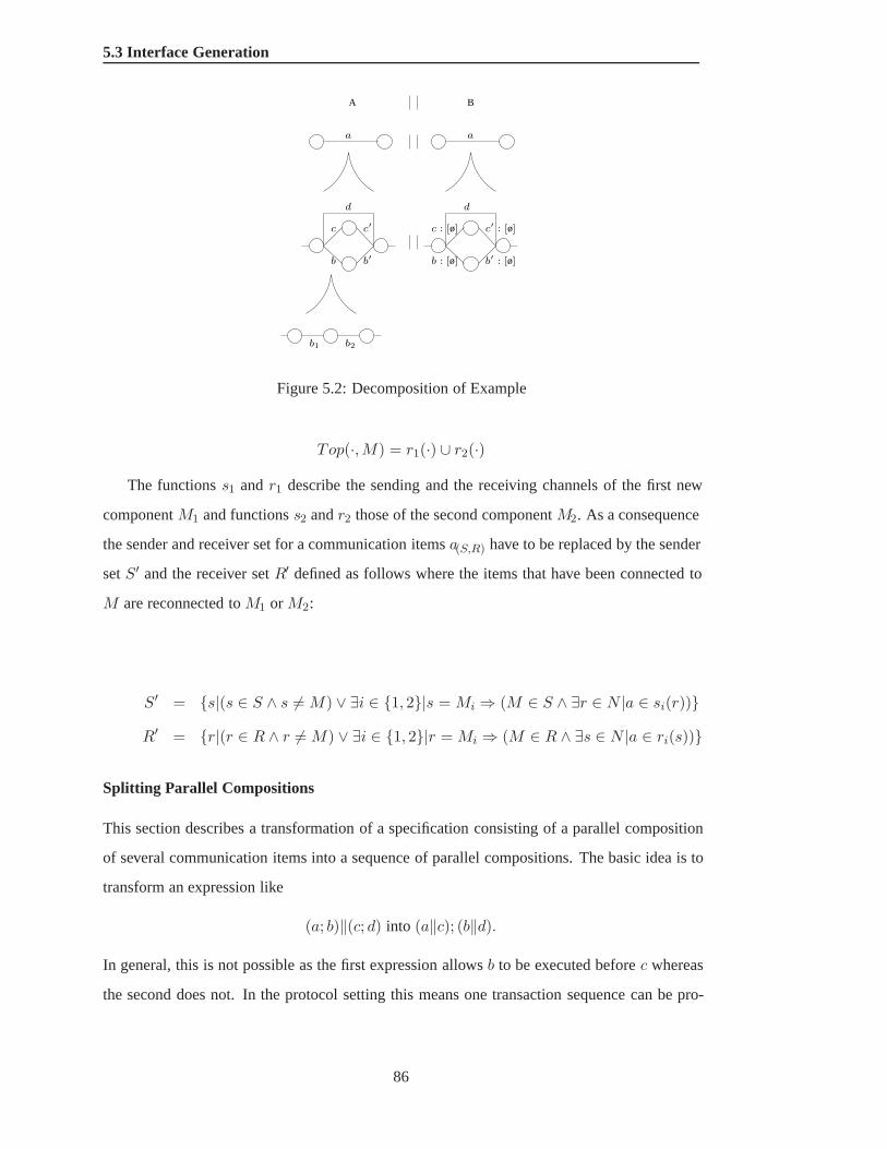
5.3 Interface Generation
a a
b2b1
A B
dd
b′
c′ c′ : [ø]
b′ : [ø]
c
b
c : [ø]
b : [ø]
Figure 5.2: Decomposition of Example
Top(·,M) = r1(·) ∪ r2(·)
The functionss1 andr1 describe the sending and the receiving channels of the first new
componentM1 and functionss2 andr2 those of the second componentM2. As a consequence
the sender and receiver set for a communication itemsa(S,R) have to be replaced by the sender
setS′ and the receiver setR′ defined as follows where the items that have been connected to
M are reconnected toM1 orM2:
S′ = {s|(s ∈ S ∧ s �= M) ∨ ∃i ∈ {1, 2}|s = Mi ⇒ (M ∈ S ∧ ∃r ∈ N |a ∈ si(r))}R′ = {r|(r ∈ R ∧ r �= M) ∨ ∃i ∈ {1, 2}|r = Mi ⇒ (M ∈ R ∧ ∃s ∈ N |a ∈ ri(s))}
Splitting Parallel Compositions
This section describes a transformation of a specification consisting of a parallel composition
of several communication items into a sequence of parallel compositions. The basic idea is to
transform an expression like
(a; b)‖(c; d) into (a‖c); (b‖d).
In general, this is not possible as the first expression allowsb to be executed beforec whereas
the second does not. In the protocol setting this means one transaction sequence can be pro-
86

5.3 Interface Generation
gressing faster than another in the parallel composition whereas in the sequential composition
this is not possible. The parallel composition allows more combinations than the sequential
one.
When the parallel composed behaviour should be implemented, especially of an interface it
is much more efficient to implement the parallel execution of several pipelines as one pipeline
that deals with parallel actions in each stage. As the mechanisms do not depend on properties of
the pipeline the proposed transformation can be generalised to pure sequences of transactions.
When parallel composition is split such that each parallel item does one item at a time those
items that take longer will block the progress of the other items. For example, the transaction
of a bus protocol that received access to the bus takes longer than a transaction that was refused
access and finishes after the unsuccessful request phase. However, as a controller component is
involved in the first communication item of all parallel transactions the sequential composition
is a possible implementation of the specification such that a new bus transaction is only allowed
after the previous one has been finished.
Generally, the transformation is possible under the condition that one component is in-
volved in one item of all parallel transactions. Then the component can delay the progress of
each parallel transaction until the others have progressed sufficiently. The parallel composition
can be split into two parallel compositions exactly at the point before the component has to
participate in the communication with all parallel transactions. This is visualised in Figure 5.3.
C involved
Figure 5.3: Splitting Parallel Composition
This means that an expression of the form (5.3) can be transformed into an expression of the
form (5.4) if there is at least one component that is a sender or receiver for all communication
itemst2i after point of splitting, formally:⋂i(S2i ∪R2i) �= ∅.
87

5.4 Implementation of Interfaces
∏i
(t1i(S1i,R1i); t2i(S2i,R2i)) (5.3)
∏i
t1i(S1i,R1i);∏i
t2i(S2i,R2i) (5.4)
If the condition is satisfied, a componentC ∈ ⋂i(S2i ∪ R2i) can ensure that for expres-
sion (5.3) the second itemst2i are only performed after the first onest1i. This is possible
because the generated interface for componentC still contains all information about all items
t1i. For example fori ∈ {1, 2}, componentC would not allow the sequencest11; t21; t12; t22
andt12; t22; t11; t21. These are the only two valid traces of expression (5.3) that are not con-
tained in the set of valid traces of expression (5.4). Hence for componentC, it is sufficient to
replace the original expression by the transformed one. Due to the synchronisation between all
system components the whole system behaves in the desired way performing the split parallel
composition.
5.4 Implementation of Interfaces
Until now the generated interfaces are fully synchronised on all actions, all components of
the system progress in the same way at the same speed. However, this does not reflect the
intention of the protocol. Components should only need to progress during communication
that is relevant to them. Therefore, this section describes the implementation of the interfaces
and how the intention of the protocol is met.
5.4.1 Dealing with Non-Relevant Items
During the decomposition of the protocol specification non-relevant items are replaced by items
that do not contain any relevant details, i.e. the details consist of the ø item. These items give
only additional information about the state of the protocol which is not necessary for the de-
scription of the communication of the component. Therefore, these non-relevant communica-
tion items can be removed altogether. Only those items remain that describe communication
in which the component is involved. Removing these items does not change the behaviour of
the interface because all communication items are still executed in synchronisation with all
88

5.4 Implementation of Interfaces
opt(a : [ø]; b) = opt(b)
opt(a; b : [ø]) = opt(a)
opt(a : [ø]; ; b) = SKIP ; ; opt(b)
opt(a; ; b : [ø]) = opt(a); ;SKIP
opt(a+ b) = opt(a) + opt(b)
opt(a ‖ b) = opt(a) ‖ opt(b)
opt(a ‖→ b) = opt(a) ‖→ opt(b)
Table 5.3: Definition of Optimisation Functionopt
other components, that means that there are no internal actions and that no component can
change its internal state. However, the description has been optimised as only relevant items
are represented.
The optimisation is described by functionopt defined in Table 5.3.
In the definition for the;; operator aSKIP item is introduced because the information
about the stages of a pipeline has to be preserved. That means non-relevant items cannot be
removed but they are replaced bySKIP items as the details are not relevant.
5.4.2 Satisfying Constraints
The constrained parallel composition operator allows the designer to easily describe behaviour
that would be error prone and tedious with the standard parallel and sequential composition op-
erator. However, when it comes to the implementation of the constrained parallel composition
extra care has to be taken that the constraints are satisfied.
If one component is involved in the communication of all items occurring in the constraint
it is sufficient that this component satisfies the constraint. As the component will synchronise
with its environment it ensures that the system as a whole satisfies the constraint. All other
components can use the parallel construct without implementing the constraint.
If a constraint cannot be satisfied by a single component several components have to imple-
89
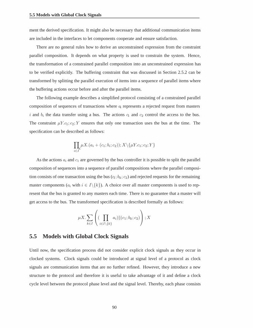
5.5 Models with Global Clock Signals
ment the derived specification. It might also be necessary that additional communication items
are included in the interfaces to let components cooperate and ensure satisfaction.
There are no general rules how to derive an unconstrained expression from the constraint
parallel composition. It depends on what property is used to constrain the system. Hence,
the transformation of a constrained parallel composition into an unconstrained expression has
to be verified explicitly. The buffering constraint that was discussed in Section 2.5.2 can be
transformed by splitting the parallel execution of items into a sequence of parallel items where
the buffering actions occur before and after the parallel items.
The following example describes a simplified protocol consisting of a constrained parallel
composition of sequences of transactions whereai represents a rejected request from masters
i and bi the data transfer using a bus. The actionsc1 and c2 control the access to the bus.
The constraintµY.c1; c2;Y ensures that only one transaction uses the bus at the time. The
specification can be described as follows:
∏i∈Ic
µX.(ai + (c1; bi; c2));X\{µY.c1; c2;Y }
As the actionsai andc1 are governed by the bus controller it is possible to split the parallel
composition of sequences into a sequence of parallel compositions where the parallel composi-
tion consists of one transaction using the bus (c1; bk; c2) and rejected requests for the remaining
master components (ai with i ∈ I\{k}). A choice over all master components is used to rep-
resent that the bus is granted to any masters each time. There is no guarantee that a master will
get access to the bus. The transformed specification is described formally as follows:
µX.∑k∈I
(
∏i∈I\{k}
ai)‖(c1; bk; c2) ;X
5.5 Models with Global Clock Signals
Until now, the specification process did not consider explicit clock signals as they occur in
clocked systems. Clock signals could be introduced at signal level of a protocol as clock
signals are communication items that are no further refined. However, they introduce a new
structure to the protocol and therefore it is useful to take advantage of it and define a clock
cycle level between the protocol phase level and the signal level. Thereby, each phase consists
90

5.5 Models with Global Clock Signals
of one or a choice of sequences of clock cycles. At the clock cycle level it is specified which
signals are driven or read in each cycle. However, there are no restrictions for the clock signals
to be used at a higher level as well.
5.5.1 Specifying Clock Cycles
During the specification clock signals can be used like any other communication items. The
specification just describes what should happen within a clock cycle. There is no verification
whether the specification can indeed be satisfied, e.g. whether all specified items fit within one
clock cycle, as communication items do not contain information about their duration. However,
it is easy to add an additional parameter that includes this information. From this augmented
specification it is possible to extract timing constraints for the clock rate. In the following
sections the duration of the communication items is considered not relevant for the functionality
of the protocol and it is assumed that the clock rate will be amended such that all timing
constraints are satisfied.
The main impact of global clock signals is that all communication items that might contain
a clock signal are relevant for all components. One could restrict the use of clock signals to
the highest modelling level and thereby allow non-relevant items at lower levels without clock
signals. However, this would mean that the highest level is already cycle accurate and the
advantages of hierarchical modelling are lost.
The solution proposed here is that clock information is represented by special communica-
tion items and the synchronisation with these clock items is handled separately. The sender and
receiver sets of clock items are equal to{clk}. These items represent certain points of the clock
cycle. The set of components is augmented with a clock component (Nclk = N∪{clk}) as well
as the set of communication items with clock items (AclkSys = ASys∪{a(S,R)|S = R = {clk}}).
As a consequence there are no relevant components for the clock signals and the advantages of
the previously described hierarchical specification method are preserved.
During optimisation of the generated interfaces these items are not rigorously removed but
the information about clock cycles is used to ensure the synchronised progress of the compo-
nents. The separate handling of clock items is justified by the fact that passing time contains
no information about the dataflow of the protocol.
The definition of the interface generation has to be amended to respect clock items as it is
91

5.5 Models with Global Clock Signals
dc′(T, a(S,R) : [SIGNAL]) = a, if R = S = clk andT a component
Table 5.4: Decomposition of Clock Signals
necessary to maintain the information about clock cycles after decomposition. Therefore, the
decomposition functiondc′ defined in Section 5.3.1 is extended to deal with the clock items as
shown in Table 5.4
5.5.2 Timing Information of Clock Cycles
While the clock signals have no other impact on the specification and interface generation as
other communication items, they affect interface optimisation and implementation in general.
In addition, the clock signals describe the concrete synchronisation points that are implicitly
defined in each communication item. They are different from the hand-over actionsı of a
pipeline because the hand-over actions are local actions of the pipeline and are still persistent
even if the stages of the pipeline are not relevant for a component. The clock signals are the
means to break down high-level synchronised actions into low-level asynchronous communi-
cation which can be directly implemented by signal drives and receivers.
As long as the specification did not contain any clock signals the optimisation of the in-
terfaces was very simple because non-relevant items could be reduced without any needs for
verification due to the synchronisation of each item. By introducing clock signals to the specifi-
cation it becomes necessary to reflect the behaviour of an item with respect to the clock signals
also in the components that are not involved in the communication of this item because the
occurrence of a clock signal affects all components.
Formally, the transformation for a system with one clock itemclk has to follow the rules
below:
a : [ø]; b = µX.(clk;X + SKIP ); b = µX.(clk;X + b)
a : [ø] + b = µX.(clk;X + SKIP ) + b = µX.(clk;X + b)
a : [ø]‖b = µX.(clk;X + SKIP )‖b
The interface has to be changed such that the component always allows time progress while
waiting for its next relevant action. The time that a component – whether participating at the
92

5.6 Summary
communication or not – has to wait is either determined by the longest time of all participating
components if these are deterministic or is described by a condition when the item has to start or
finish. The exact number of clock items to be introduced can only be determined by analysing
all components.
5.5.3 Implementing Synchronisation
With clock items it is possible to implement synchronisation asynchronously as it is physically
realised using signal drivers and receivers.
The synchronisation information of parallel composed communication items is only needed
when decomposing the system to ensure synchronisation takes place. While synchronisation
is abstract on the higher levels it becomes concrete on the signal level by establishing com-
munication. Communication is implemented by the senders driving a signal and the receivers
reading the signal line at the same time. The clock signals give indications for the sender, resp.
receiver, when the receiver, resp. sender, will perform its part of the synchronisation. If a re-
ceiver performs its part of the action while the sender does then it is said that the action took
place in synchronisation of sender and receiver.
5.6 Summary
The framework presents a methodology to model hardware communication protocols. The
main emphasis was to provide an intuitive and general as well as formally defined design
method. The three stages in the design process are summarised below:
1. The designer starts with a high-level specification of possible protocol transactions and
refines them stepwise until a signal-level specification has been created. There is no need for
verification for these steps.
2. After the specification protocol interfaces are generated. Any specification level can be
used to create the interfaces. Each interface reflects the specified transactions to the details that
the interface is generated for.
3. The generated interface can be optimised using further refinement steps that have to be
verified if necessary. These optimisations can use information about the state of the protocol,
the suggestions of the designer about the implementation, e.g. pipelines, and resolve constraints
93

5.6 Summary
that would need additional logic.
94

Chapter 6
Case Study: PI-Bus
In this chapter the framework described in the previous chapter is applied to the transactions
specified in the open-source PI-bus protocol [60]. This protocol defines the communication
between master and slave components via an on-chip bus connection. The bus is controlled by
a bus control unit.
In a first attempt the different phases of a bus transaction have been modelled as individual
processes that are connected using the conditional choice construct described in Chapter 3.
However, this approach does not allow to conveniently model pipelines because the phases
of one single transaction can not be easily identified. For each transaction the same phase
description is used. While this seems to be good at first sight it proves to be inconvenient to
describe sequences of transactions. For example, it becomes difficult to describe a transaction
that is aborted and a transaction that goes through the address and data phases more than once
using the same phase descriptions. In contrast, the data flow approach allows to describe each
transaction and each phase of a transaction individually while specifying the behaviour of all
system components at the same time. Hence, the latter approach developed in the framework
is more appropriate for these protocols than the pure process algebraic one.
In the next section a general transaction between one master and one slave component is
specified and refined down to signal level. When the protocol specification for the interleaving
of transactions is described later on, annotations to the general transaction are introduced to
distinguish between different components.
95

6.1 Protocol Specification
6.1 Protocol Specification
6.1.1 Transaction
The PI-bus protocol describes two bus transaction types, namely read and write transactions.
They can be performed with data of different lengths. A third type, so-called split transactions,
where the bus is released during a transfer, are optional and not fully defined in the standard.
Typically, several transactions can be ready for execution. However, only one of these will
be granted access to the bus at any one time. After the bus has been granted, data can be
transferred. All transactions that were not granted the bus are cancelled and their requests have
to be performed again as new transactions.
The behaviour described in the previous paragraph should be intuitively stated at trans-
action level. All other details are not relevant at the moment. They are summarised as one
communication item, e.g. in a transaction the data transfer is represented by an item named
transfer , and are defined later. This has the additional advantage that all transaction types can
be described with the same high-level specification. Hence, a transaction can be described by
the following expression:
transaction = request ;
(no bus granted+ (6.1)
(bus granted ; ; transfer ; bus release))
In the above description, the itemsno bus granted andbus granted are used to explicitly
model the choice of which transaction will be granted the bus. The itembus granted, resp.
no bus granted, would be used in the description of the whole protocol such that the bus
control unit does, resp. does not, grant the bus to the master that drives this transaction1.
1In the PI-bus specification one signalgnt per master is used which indicates whether the bus has been granted.
As value passing has not been introduced into the design language two signals (bus granted andno bus granted)
are used here instead.
96

6.1 Protocol Specification
6.1.2 Phase-Level Modelling
A transaction consists of a combination of three phases, the request phase, which is already
used in the definition of atransaction , the address and the data phase. The address and data
phases are only relevant if the bus has been granted and therefore are only used in the descrip-
tion of the details oftransfer items. There can be several address and data phases during one
transfer, but they are always paired and the address phase always has to finish before the corre-
sponding data phase starts. As the protocol allows the transfer of several data during one trans-
action there are two possibilities during a transfer. First, the transfer just finishes with a data
phase, hereafter denoted bytransfer data , or second, the data phase is performed potentially
overlapped with a newtransfer data . The hierarchical refinement oftransfer representing
these two possibilities is given below.
97

6.1 Protocol Specification
transfer : [transfer details ]
transfer details = transfer data + (transfer data ‖→ transfer details)
transfer data : [address ; ; data ]
The transfer finishes after the last data phase has been executed, i.e. the choice has been
resolved in favour of a single transfertransfer data .
In the protocol standard the request phase also contains the grant signalsbus granted and
no bus granted . However, these signals can not be included into the request phase within this
modelling framework because the phase level would hide these grant signals on the transaction
level whereas they are needed to control which transaction may proceed and start the transfer
of data.
An advantage of this hierarchical refinement approach is that at this level the specification
still abstracts from the signal-level implementation. The description of the transfer at the phase
level makes clear in which order address and data phases may occur without giving signal-level
details of the phases. Each phase can subsequently be refined to signal level as shown in the
following section.
6.1.3 Signal-Level Implementation
Finally, it remains to define which wires are used for communication in each phase. The
hierarchical modelling allows to define each phase independently of the other phases. The
request phase just uses one request signal and, hence, does not need further refinement. Its
details are described by the signal itemSIGNAL:
request : [SIGNAL]
In the address phase the bus can be locked (lock ), the length of data is specified (opc),
the type of transaction is communicated (read ) and the address (addr ) of the slave is de-
fined. These four actions are performed by driving signals, therefore they are defined as
lock : SIGNAL, etc. For simplicity reasons the actions are executed sequentially, although
the protocol description does not specify any ordering. If it is necessary to model all possible
sequences one would use the parallel operator instead of the sequential operator.
98

6.1 Protocol Specification
12
3
45
6Master Slave
Controller
Figure 6.1: Routing Plan for High-Level Signals
address : [lock ; opc; read ; addr ]
The data phase consists of sending data (dbus) and an acknowledgement (ack ) signal. For
read transactions the acknowledgement is sent before the data is transmitted. In case of a
negative acknowledgement, i.e. a wait or an error value has been sent as acknowledgement, the
data is not sent and a timeout might occur. Hence, the data phase of the read transaction can
drivedbus or timeout or do nothing after the acknowledgement, formally:
data : [ack ; (dbus + timeout + SKIP)]
For write transactions the specification looks similar butack anddbus can occur in any
order.
6.1.4 Topology
After the communication behaviour of the PI-bus protocol has been specified, the topology of
the system needs to be defined. The topology states which system components are connected
by which items and in which direction the data flows. In contrast to other design methods
where the behavioural description defines the system components, here, the topology can be
defined independently of the behaviour.
Table 6.1 shows which system components participate at which items. It can be used to
generate a routing plan for the protocol signals as shown in Figure 6.1 for the first six high-
level signals of Table 6.1 denoted by 1 to 6 in the figure.
99
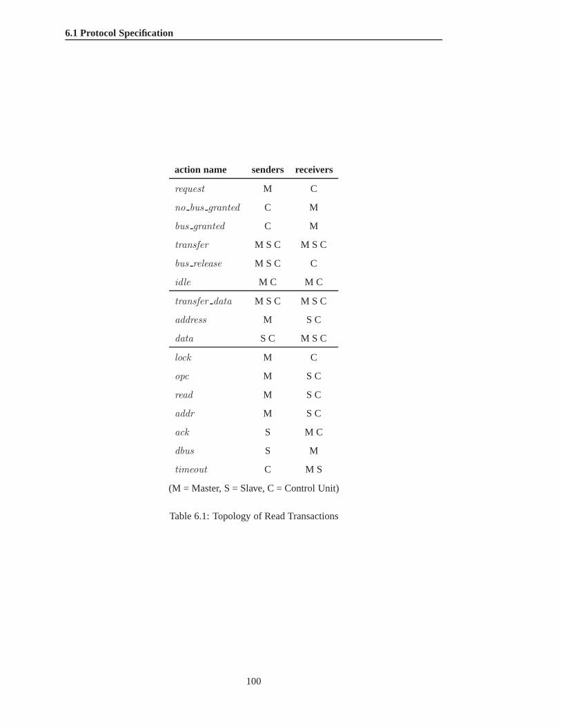
6.1 Protocol Specification
action name senders receivers
request M C
no bus granted C M
bus granted C M
transfer M S C M S C
bus release M S C C
idle M C M C
transfer data M S C M S C
address M S C
data S C M S C
lock M C
opc M S C
read M S C
addr M S C
ack S M C
dbus S M
timeout C M S
(M = Master, S = Slave, C = Control Unit)
Table 6.1: Topology of Read Transactions
100

6.1 Protocol Specification
6.1.5 Top-Level Specification
In the previous section one transaction between a specified master and slave component has
been described. In order to model the general case where several transactions between different
master (M ) and slave (S) components take place a parametrised version of the above described
transaction has to be used.
transaction = transaction(M,S)
To each communication item a parameter is appended that indicates which master and
which slave is involved in this transaction. Later, during the optimisation phase, the bus signals
of several transaction, e.g.dbus, addr will be identified as one single communication item.
As already mentioned the bus can be used just by one transaction at a time. It is the
controller’s task to satisfy this property by selecting the master that drives this transaction.
One has to decide how to implement the property that only one transaction is using the
bus at a time. One possibility is to constrain the parallel composition of all transactions. The
constraint would specify that bus grant and release items have to alternate using items of the
details of the transaction item. This is problematic as the details are not specified yet, thus, no
action names are known.
The second possibility would be to model the grant and release items explicitly on the
transaction level and split a transaction into two parts, one before the grant item and the other
part in between grant and release items. Thereby, the transaction does not introduce a new
hierarchy level, it is just a composition of communication items. The communication items for
the transaction are reused unchanged in the protocol specification, annotated with parameters
indicating between which components the transaction takes place.
The protocol definition for master componentsMi and slave componentsSj with i, resp.
j in index set∈ IM , resp.∈ IS is shown below. It consists of a parallel composition of
transactions that is constraint by a conditionc. This condition has to ensure that the bus is only
used by one transaction at a time.
protocol =∏i∈IM
trans sequence(i)\{c} (6.2)
trans sequence(i) = (∑j∈IS
transaction(Mi ,Sj ) + idle) ‖→ trans sequence(i)
101

6.2 Interface Generation
transaction(Mi ,Sj ) = requesti ;
((no bus grantedi )+ (6.3)
(bus grantedi ; ; transfer(Mi ,Sj ); bus releasei ))
In the constraintc the communication itemsrequesti , no bus grantedi , bus grantedi ,
transfer , bus releasei can be used to express that only one transaction should use the bus
at the time. As it is assumed that there is a default master the case that no master is granted the
bus does not have to be described. The constraint consists of two parts that are repeated. The
first partc1 describes that only one masteri ∈ IM is granted the bus, the second partc2 that no
master is granted the bus until the bus is released. As both parts use the information about the
masteri currently using the bus they take a parameteri. Altogether the constraint looks like
the following:
c1(i) = bus grantedi‖∏
j∈IM\ino bus granted(j)
c2(i) = (∏
j∈IM\ino bus granted(j))∗; bus releasei
c =
∑i∈IM
c1(i); c2(i)
∗
The constraint can be satisfied by the controller of the bus. The interface for the controller
will be transformed from a specification that uses parallel constructs into a specification that
describes the protocol in sequences. This is described in the following section about the con-
troller interface.
6.2 Interface Generation
From the information given above it is now possible to generate interfaces for the master,
slave and controller component by decomposing the protocol description with respect to the
corresponding component.
102
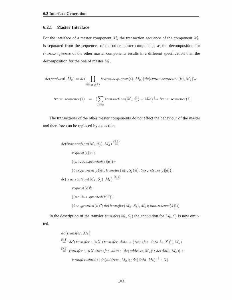
6.2 Interface Generation
6.2.1 Master Interface
For the interface of a master componentMk the transaction sequence of the componentMk
is separated from the sequences of the other master components as the decomposition for
trans sequence of the other master components results in a different specification than the
decomposition for the one of masterMk.
dc(protocol,Mk) = dc(∏
i∈IM \{k}trans sequence(i),Mk)‖dc(trans sequence(k),Mk)\c
trans sequence(i) = (∑j∈IS
transaction(Mi ,Sj ) + idle) ‖→ trans sequence(i)
The transactions of the other master components do not affect the behaviour of the master
and therefore can be replaced by a ø action.
dc(transaction(Mi, Sj),Mk)(5.1)=
request(i)[ø];
((no bus granted(i)[ø])+
(bus granted(i)[ø]; transfer(Mi ,Sj )[ø]; bus release(i)[ø]))
dc(transaction(Mk, Sj),Mk)(5.1)=
request(k)!;
((no bus granted(k)?)+
(bus granted(k)?; dc(transfer(Mk ,Sj ),Mk ); bus release(k)!))
In the description of the transfertransfer(Mk ,Sj ) the annotation forMk, Sj is now omit-
ted.
dc(transfer ,Mk )(5.1)= dc′(transfer : [µX .(transfer data + (transfer data ‖→ X ))],Mk )
(5.2)= transfer : [µX .transfer data : [dc(address,Mk ); ; dc(data,Mk )] +
transfer data : [dc(address,Mk ); ; dc(data,Mk )] ‖→ X ]
103

6.2 Interface Generation
dc(address,Mk ) = address! : [lock !; opc!; read !; addr !]
dc(data,Mk ) = data? : [ack?; (dbus? + timeout? + SKIP)]
As the master component is involved in every communication of its transaction sequences
all actions are represented in the interface of the component.
Implementation
The interface for the master still contains information about other master components. As
theses are not relevant they can be removed following the optimisation described on page 89.
dc(transaction(Mi, Sj),Mk)opt= ø
Assuming that the controller will ensure that the constraint is satisfied the implementation
of the master does not deal with the constraint. That means that the final interface for the master
component looks like the following:
dc(protocol ,Mk) = dc(trans sequence(k),Mk)
6.2.2 Slave Interface
In the transaction sequences driven from any master component there can be a transaction with
which the slave componentSk is involved. Therefore, all parallel processes remain persistent
but the choice within a transaction sequence is split into those transactions with slaveSk and
those with other slaves.
dc(protocol, Sk) = dc(∏i∈IM
trans sequence(i), Sk)\c
trans sequence(i) =((
∑j∈IS\{k}
transaction(Mi ,Sj ) + idle)+
transaction(Mi ,Sk ))
‖→ trans sequence(i)
104

6.2 Interface Generation
The transactions driven by master components to other slave components do not affect the
behaviour of the slave and therefore can be replaced by a ø action. There is only one branch of
the choice over the transaction sequences which involve the slave componentSk.
dc(idle, Sk) = idle[SKIP ]
dc(transaction (Mi, Sj), Sk)(5.1)=
request(i)[ø];
((no bus granted(i)[ø])+
(bus granted(i)[ø]; transfer(Mi ,Sj )[ø]; bus release(i)[ø]))
dc(transaction (Mi, Sk), Sk)(5.1)=
request(i)[ø];
((no bus granted(i)[ø])+
(bus granted(i)[ø]; dc(transfer(Mi ,Sk ),Sk ); bus release(i)!))opt=
ø; ((no bus granted(i)[ø])+
(bus granted(i)[ø]; dc(transfer(Mk ,Sk ),Sk ); bus release(i)!))
The choice whether the bus is granted or not only influences the behaviour of the slave
component at the first sight. When analysing the whole behaviour, the slave has to wait until
a master has been granted the bus and the transfer starts. Therefore, the whole transaction
sequence reduces to a sequence of transfers (6.4) after optimisation.
dc(trans sequence(i), Sk) = (6.4)
dc(transfer (Mk, Sk), Sk)‖→ dc(transfer (Mk, Sk), Sk)
For the slave the topology of the system specifies that it has to be ready only for the transfer
of data. In the decomposition of the transaction with respect to the slave this is reflected by
one ø action for the details of the non-relevant actions, i.e. the actions in which the slave is not
involved.
The refinement oftransfer is similar to the one of the master component, only the direction
of some actions is changed and thelock action is replaced by a ø action.
105

6.2 Interface Generation
Implementation
All transactions the slave componentSk is not involved in can be reduced to a ø according to
the definition of the optimisation function on page 5.4.1.
dc(transaction(Mi, Sj), Sk)opt= ø
As the controller ensures the satisfaction of the constraint the final interface for the slave
looks like the following:
dc(protocol , Sk) =∏i∈IM
dc(transfer (Mi, Sk), Sk)‖→ dc(protocol , Sk)
6.2.3 Controller Interface
The controller is involved in any transaction. Therefore, the whole structure of the protocol
remains persistent.
dc(protocol, C) =∏i∈IM
dc(trans sequence(i), C)\c
trans sequence(i) = (∑j∈IS
transaction(Mi ,Sj ) + idle) ‖→ trans sequence(i)
dc(transaction(Mi, Sj), C)(5.1)= request(i)?;((no bus granted(i)!)+
(bus granted(i)!; transfer(Mi ,Sj ); bus release(i)?))
However, the constraint can be used to simplify the transaction as the controller can resolve
the choice of which master is granted the bus in accordance to the constraint.
In a first step, the choice is moved over the slave components inside of the transaction de-
scription. This was not useful for slave and master components as only some of the transactions
were relevant for the components. The controller is involved in all transactions with any slave.
106

6.2 Interface Generation
The second step is more substantial. The parallel composition of transaction sequences is
translated into a sequence of parallel communication items as described in Section 5.3.2.
The controller is involved in the request item of any transaction and therefore it is possible
to split the parallel transaction sequences into sequences of parallel transactions.
∏(µX.(transaction ‖→ X)) = µX.(
∏(transaction) ‖→ X)
In the third step, the parallel transactions∏
(transaction) are split into a sequence of
parallel items. As the controller is involved in thebus granted andno bus granted signal
the transaction can be split before the choice in each transaction. Schematically, the operation
consists of a transformation between
∏(request?; (no bus granted + (bus granted ; ; transfer ; bus release)))
and
∏(request?);
∏(no bus granted + (bus granted ; ; transfer ; bus release))
The result of the two splitting transformations is that the Expression 6.6 is transformed into
Expression 6.7 as given below.
∏µX .request?; (no bus granted+ (6.5)
(bus granted ; ; transfer ; bus release)) ‖→ X
µX .((∏
request?);∏
(no bus granted+ (6.6)
(bus granted ; ; transfer ; bus release)))
‖→ X
The transformation described in the previous subsection simplifies the way to satisfy the
constraint of the outermost parallel composition in the specification. It remains to introduce a
conditional choice that resolves the choice betweenbus granted andno bus grant accord-
ingly to the constraint. The condition is expressed bybus available?. Altogether the descrip-
tion is as follows:
dc(protocol, C, bus available?) =
107

6.3 Clock
∏i∈IM
request(i)?; ((bus available?) :
( ∑k∈IM
(∏
i∈IM \{k}no bus granted(i)!‖
bus granted(k)!); ;∑j∈IS
transfer(Mk ) ‖→ dc(protocol ,C , false))#
( ∏i∈IM
no bus granted(i)! ‖→ dc(protocol ,C , false ))
6.2.4 Composition
Placing the components into a parallel composition results in a description behaviourally equiv-
alent to the first specification of the protocol given in (6.2) in accordance to the definition in
Section 5.3.1.
protocol �∏i∈IM
dc(protocol ,Mi ) ‖ dc(protocol ,C ) ‖∏j∈IS
dc(protocol ,Sj )
where the synchronisation sets are the intersection of the alphabets of the components of the
parallel composition.
6.3 Clock
6.3.1 Specification
So far the protocol has been specified without using clock signals. Using this specification the
clock cycles can be defined by the phases which each take one clock cycle. The clock signals
are added at the end of each phase. The specification with clock is stated below:
protocol =∏
trans sequence\{c}trans sequence = (
∑transaction + idle) ‖→ trans sequence
transaction = request ; ((no bus granted ; clk)+
(bus granted ; clk ; ; transfer ; bus release))
transfer = transfer : [µX .(address; clk ; ; data; clk)+
(address; clk ; ; data; clk) ‖→ X ]
108

6.3 Clock
It differs from the original only by the additionalclk items with which the components
have to communicate. The decomposition is built using the functiondc in the same way as
described in the previous section.
6.3.2 Implementation
At the highest level of the PI-bus specification the clock affects only the optimisation of the
slave components. The master and controller components are involved in at least one commu-
nication item of each phase and therefore their interfaces do not have to deal with empty clock
cycles.
For the slave component the itemsidle andrequest are not relevant. In the un-clocked
case this allows the reduction to
transfer ‖→ transfer
for a single slave component. In the clocked case there can be severalclk signals before the
first transfer with this slave starts. Therefore, empty clock cycles have to be introduced where
time just passes and the component does nothing but is able to synchronise on theclk signal as
described in Section 5.5.
When the rules for interface generation are applied to the slave component then its interface
looks like the following:
dc(protocol ,Sk ) =∏trans sequence\{c}
trans sequence = (transaction + idle) ‖→ trans sequence
transaction =
µX .(clk ;X + SKIP);
((µX .(clk ;X + SKIP); clk)+
(µX .(clk ;X + SKIP); clk ; ; transfer ; bus release)) =
µX .((clk ;X + clk);SKIP + transfer ; bus release))
transfer = addr ; clk ; ; data; clk
109

6.4 Conclusions
The transaction sequence can be simplified by summarising the empty clock cycles:
trans sequence = µX .((clk ;X + clk ;SKIP); transfer ; bus release)
6.4 Conclusions
The presented example shows how interfaces for system components can be derived from a
single specification. The interfaces are generated automatically and they bear the same hier-
archical structure as the specification. A further advantage is that the method is modular. In
principle, further refinements could be done in the same systematic way. As long as the rules
are applied correctly the resulting interfaces are compatible with each other. In that sense, the
method applied is correct-by-construction.
The resulting model can be used for analysis and synthesis purposes. It is as accurate as
signal-level VHDL description and therefore, could be directly synthesised using transforma-
tion rules similar to C-to-VHDL converters like SPARK [63]. However, the focus of the work
is on the improvement of the specification methods, not on synthesis.
110

Chapter 7
Conclusions
7.1 Summary
This research project was guided by the challenge to find a better way to model communication
protocols like the PI-bus protocol. The introduction of the conditional choice based on previous
behaviour was a first step towards a better support for the modelling of protocol phases. The
idea was that possible behaviours for a component during a phase are modelled separately and
then combined using the choice operator. Based on the previous behaviour the choice has been
restricted to the valid behaviours for the actual state of the protocol. This construct was first
realised in process algebras.
However, the conditional choice construct does not model pipelines conveniently because
the construct merges the description of data transfers with the definition of pipeline stages. It
becomes difficult to model the protocol because transactions passing through a pipeline are
not easily identified. Dataflow algebras can provide the distinction between the data and the
architecture of the system. The challenge is to combine both approaches in one theoretical
framework.
Additionally, the aim of the research project was to bridge between the theoretical aspect of
specifications and industrial design aspects. The most interesting approach used for industrial
applications was SystemCSVdescribed in Section 2.6. The hierarchical approach seems to be
predestinated to represent communication. However, no formal foundation existed prior to the
presented thesis that provides such a foundation for the hierarchical modelling approach.
111

7.1 Summary
The framework presented in this thesis provides a method to specify communication proto-
cols in a formal and intuitive way. It allows to describe a high-level system specification and to
derive a refined specification in a hierarchical manner. It excludes ambiguities by a rigorously
defined semantics that not only defines the communication behaviour between the system com-
ponents but also includes all modelling levels. This consistent hierarchical way of modelling
ties together and even intermixes specification and implementation. The verification gap be-
tween specification and implementation is minimised. Action refinement has been exploited as
a theoretical basis for hierarchical modelling within the framework.
Furthermore, new operators have been introduced to the design language to allow mod-
elling pipelines conveniently. An approach based on dataflow has been taken such that transac-
tions of a protocol can be described from a system-wide viewpoint. This is different to process
algebras, where the focus of the modelling is on the behaviour of individual components and
therefore extra precaution has to be taken to ensure compatibility between components.
The presented framework brings together the benefits of process algebra and dataflow al-
gebra. It presents a link between the needs of high-level specification of protocols realised
by dataflow algebra and the needs of behaviour-oriented, imperative descriptions of protocol
interfaces which are better modelled in process algebras or state-based languages. This link
goes beyond the restriction of dataflow algebra terms because a formal relationship is defined
between dataflow-algebraic and process-algebraic models which have different semantics.
Formal state-based languages, such as Petri nets, have not been used because communica-
tion protocols are better understood by describing their behaviour. Obviously, protocol states
are used to identify behaviour. However, for the definition of a protocol the nature of commu-
nication protocols suggests itself to use a description of how the system progresses instead of
a collection of state variables.
First attempts using pure behavioural descriptions without the concept of dataflow have not
been very fruitful. The conditional choice construct based on previous behaviour resulted from
such an early attempt to improve pure process algebraic descriptions for protocols. The goal
was to represent each protocol phase as a single process. Then, the protocol process would
consist of a composition of the phase processes. In order to reuse the same phase process under
different conditions the conditional choice construct is used. It simplifies the process and makes
it easy to understand. The conditions, e.g. whether the bus has been granted or not, or whether
112

7.1 Summary
the slave could deliver data in time or not, are explicitly described as dataflow. Attempts to
unroll the conditions led to large processes and it was difficult to find a general solution for
all conditions. Furthermore, this approach did not extend to pipelines. As mentioned above, it
merged the specification and implementation of pipelines such that it was difficult to distinguish
between implementational details like the hand-over and the high-level description of protocol
phases.
7.1.1 Comparison with Similar Approaches
In comparison to the work by Seidel [58] about the compatibility of an early version of the PI-
bus protocol the framework presented in this thesis could indeed improve the modelling of the
protocol. Seidel models the PI-bus in CSP but the intended pipeline structure of the protocol
implementation could not be captured within the language. Furthermore, the different phases
of a transaction could not be easily identified or altered as parts of them were spread over the
whole specification.
Herrmann and Krumm present a framework for modelling transfer protocols [37, 38], here
for short FFMTP. It consists of a collection of predefined, parametrised modules that facilitate
the formal specification of protocols and service constraints. The FFMTP comprises each
typical functional property of data transfer services as well as basic protocol mechanism and is
therefore limited to the predefined modules and not as general as the presented framework in
this thesis.
A complete protocol description in FFMTP consists of a combination of service constraints
and a separate combination of protocol mechanisms. FFMTP provides proofs for valid com-
binations of protocol mechanisms that satisfy a given service constraint. These proofs have
been generated manually and use an intermediate level between service constraints and basic
protocol mechanisms. Users of FFMTP have to provide proofs for their models and service
constraints based on the proofs provided by the framework. The verification of the correct re-
lation between the specification and the model is then performed in two major steps: from the
specification to the intermediate level and from the intermediate level to the service constraints.
The approach of Herrmann and Krumm is closer to a construct-by-correction approach
as users of FFMTP have to iteratively redesign their model until a proof can be found. In
contrast, the presented framework can be called a correct-by-construction approach because
113

7.1 Summary
the resulting model can directly be related to the top-level specification and is in the sense of
this relationship correct.
Furthermore, the design language of FFMTP is a variant of Lamport’s temporal logic of
actions [44] which requires the designer to express the specification in logical formulae instead
of a behavioural description as done in this thesis.
Oeberg presented a similar modelling approach to the framework in this thesis. He defined
theProGram system [52] for hardware synthesis. The system provides synthesis rules from a
grammar-based specification and returns VHDL code at register-transfer-level. It separates the
communication description and the behavioural description similar to the dataflow approach.
However, the system has been developed to explore lower-level design issues. For example,
the impact of different port widths can be analysed using ProGram. Furthermore, hierarchical
design is not supported.
7.1.2 Hierarchical Modelling
On one hand hierarchical modelling allows the designer to abstract from details that are de-
fined on lower levels. On the other hand hierarchical modelling allows the designer to focus
separately on each particular aspect when modelling the lower-level details. The designer does
not have to think about the influence of the details onto the whole system.
It is only possible to take advantage of this approach if a naturally and easy to understand
hierarchy is present in the system that has to be modelled. In the case of communication
protocols the hierarchy is given by the composition of lower-level communication items to
meaningful higher-level communication items.
The constrained parallel composition makes it difficult to maintain a rigorously defined
hierarchy because the level used for the parallel composition might not provide enough details
to express conditions for high-level parallel composition of communication items. In the case
of the PI-bus the granting of the bus cannot be represented at transaction level. In the protocol it
is described by the grant signal. In order to use the bus granting in a constraint it is necessary to
artificially introduce a high-level item that represents the grant and release of the bus. Later in
the design process the grant item is refined to the original signals creating an hierarchical item
that represents just a signal. The bus-release item does not have a physical representation and
is therefore not relevant for the implementation. Due to the hierarchy and the lack of details at
114

7.2 Future Work
higher levels it is necessary to introduce these items explicitly.
7.1.3 Time
The framework only deals with abstract time. Abstract or discrete time is only concerned
with distinct time events like clock signals. This representation of time is suitable for higher-
level specification and globally synchronised systems such as bus architectures. Discrete time
models produce qualitative rather than quantitative information. However, it has been shown
that the discrete time events can be used as counter e.g. for the duration of an action [17].
Generally, clock signals in behavioural descriptions have a semantics that differs from nor-
mal actions. For example in process algebras, normal actions can have priority over clock
signals. However, considering dataflow, the specification treats communication items equally
to time progress. Extra treatment for clock signals has been introduced only for convenience
in order to better support hierarchical modelling.
The clock signals that are contained in the generated interfaces indeed indicate passing
time. It can be argued that, therefore, these actions have to be treated differently. However,
as the framework is intended to generate specifications instead of executable models the clock
signals represent information similar to communication actions. Finally, at signal level clock
signals are sent via wires as well.
The clock signals can be used to extract information about the required clock frequency
and the signal driver specification. This aspect involves the physical properties of the com-
munication architecture and has not been covered in this research as it would need orthogonal
extensions to the design language.
7.2 Future Work
7.2.1 Tool Support
The framework should be supported by a collection of tools, that further simplifies the spec-
ification and modelling process. Visual editors should allow the designer to browse the hier-
archical description of the model. Unspecified communication items should be identified and
checks for the scope of names performed.
115

7.2 Future Work
Furthermore, interfaces to verification tools such as model checkers should be provided to
increase the confidence in the model as well as to verify implementation steps such as removing
constraints.
A different application of the framework would be as a simulation stimulus generator. The
models of one or more components can be used to simulate communication that is conform to
the protocol without having to specify the remaining system. Due to the hierarchical modelling
approach, the components do not have to be specified in full detail as the protocol interface can
be generated at any hierarchy level.
Finally, automated generation from an implementation to synthesisable hardware descrip-
tion languages would be desirable.
7.2.2 Semantics of Dataflow Algebra
In the presented framework the semantics has been defined using the valid/invalid trace se-
mantics of dataflow algebra and the operational semantics of process algebra. Further work
has to be done to generally relate the valid/invalid trace semantics to the semantics of process
algebras.
As the topology of the system is fixed the semantics is not assumed to be compositional.
Although this is an important property for process algebra this property is not relevant and has
not been investigated in the presented framework.
Dealing with constraints, used in constrained parallel composition, is vital in the modelling
of interleaved protocol transactions. Constraints introduce a different composition of traces,
namely intersection, which makes a translation to operational semantics difficult. In the frame-
work the resolution of constraints has been referred until the interfaces are implemented. The
resolution needs manual verification, which is not very satisfying. A solution would be to in-
troduce constraining processes that are composed in parallel to the components as it has been
done for the conditional choice based on previous behaviour. However, these constraints are
rarely implemented as parallel components. Instead, registers and additional logic are used
most commonly. Therefore, the framework leaves the resolution of constraints to the designer.
116

7.3 Further Application Areas
7.2.3 Low-level Communication
The implementation of generated interfaces of a protocol has been described down to the signal
level. All signals have been described and sender and receiver of a signal have to perform their
part of the communication in synchronisation.
However, systems-on-chip usually do not provide such a synchronisation mechanism. The
sender and receiver of a signal are just connected by one or more wires. The clock signals are
used to synchronise the components. This aspect has not been described as it would require
information about the physical properties of the system.
With additional information about how long a signal is driven and how long a wire is
sampled it would be possible to extend the framework such that the low-level unsynchronised
communication can be modelled.
In order to support unsynchronised communication it would be necessary to introduce as
many clock signals representing time points in the clock cycle as required to capture the du-
ration of the sending and receiving signals. Usually three clock signals are sufficient to mark
time pointsearly, half andlate in the clock cycle. Additionally, the synchronised parallel com-
position operator has to be replaced with the interleaving parallel composition operator. Then,
during a further implementation step of the protocol interfaces, the send and receive action can
be shifted into different slices of the clock cycles in order to respect the latencies of wires and
drivers.
7.3 Further Application Areas
7.3.1 Protocol Bridges
The generation of protocol interfaces is in particular interesting for components where the
behaviour of the component is only defined by the protocol itself and no further implementation
is necessary. For example, the bus controller is such a component. For these components
it would be possible to synthesise them without requiring any further information about the
behaviour.
Taking it a step further, bus protocol bridges, i.e. the connection between two bus architec-
tures, could be specified and synthesised in a similar way as the task of a bridge can be defined
117

7.3 Further Application Areas
universally. However, the challenge for the automated synthesis consists of integrating two
interfaces to different protocols.
It might also be interesting to investigate properties of the separately generated protocol
interfaces for both protocols of the bridge and deduce properties of the whole system, e.g.
duration of communication or possible deadlocks.
7.3.2 Performance Analysis
At the beginning of the research project, performance analysis of protocols for systems-on-chip
has been investigated. Probabilistic process algebras have been shown to be helpful for perfor-
mance analysis, e.g. [36]. In the context of communication protocols, it would be possible to
calculate approximate performance values based on latency of wires, estimates for the traffic
and the behaviour of the system components.
However, the tasks of modelling protocols needs accurate information and the behaviour of
protocols, in contrast to components, cannot be approximated using probabilities. Therefore,
the probabilistic approach has been abandoned and the focus was on the functional verification.
As the protocols are deterministic the performance of a system using a protocol is better
calculated using methods like counting clock cycles, [17]. Based on these calculations it would
be possible to analyse the performance of the whole system. This approach would be more
suitable than modelling the protocol in probabilistic process algebra because it clearly separates
estimations of the components and deterministic behaviour of the protocol.
118

Appendix A
VHDL-like Specification Language
The specification language of the framework in this thesis was presented in an algebraic syntax.
In order to make the language accessible to non-theoreticians the language has been translated
to a VHDL-like syntax.
The concept of communication items nicely translates the VHDL constructs forENTITY
andPROCESS. The declaration of a communication item with its ports is described as a com-
munication entityCOM ENTITY. The ports are described byPORT whereOUT denotes the
senders of this item andIN the receivers. The details of a communication item is described as
a communication processCOM PROCESS:
COM ENTITY transaction IS
PORT (master, controller:OUT;
slave:IN)
END transaction;
COM PROCESS OF transaction IS
BEGIN
req;
addr;
data;
END transaction;
119

VHDL-like Specification Language
The sequential composition operator is denoted by the original operator (;). The parallel
composition and constraint parallel composition use the VHDL constructPAR ... END
PAR where the composed items are separated byAND. Similarly, overlapping, potentially
pipelined items are enclosed byOVERLAP andEND OVERLAP and the stage operator;; re-
mains unchanged. For the choice operator the VHDL constructSELECT has been used. The
repetition of a process is declared byREPEAT ... END REPEAT.
PAR [CONSTRAINT ... END CONSTRAINT]
... AND ...
END PAR;
OVERLAP
trans-1 AND
trans-2
END OVERLAP
SELECT t-1 OR s-1 END SELECT
The process declaration of signals and partly specified items just consists of aSIGNAL or
SKIP item.
COM PROCESS OF acknowledge IS
BEGIN
SIGNAL
END acknowledge;
COM PROCESS OF transaction IS
BEGIN
SKIP
END transaction;
120

VHDL-like Specification Language
For convenience a choice or a parallel composition over an index setI can be described
using the extensionSELECT OVER i ∈ I... or PAR OVER i ∈ I. Using indentation
gives a specification a better structure. For example a simplified version of a protocol could be
described as follows where requests are described bya-i, transfers byb-i and control signals
by c-i:
REPEAT
SELECT OVER J ⊂ I, j ∈ J
PAR OVER i ∈ J
a-i
END PAR;
c-1;
b-j;
c-2
END SELECT
END REPEAT
121

Bibliography
[1] A. Aho, R. Sethi, and J. Ullman.Compilers, Principles, Techniques and Tools. Addison-
Wesley Publishing Company, 1986.
[2] R. Back and R. Kurki-Suonio. Decentralisation of process nets with centralised control.
2nd ACM SIGACT-SIGOPS Symposium on Principles of Distributed Computing, pages
131–142, 1983.
[3] J. Baeten and J. Bergstra. Process algebra with signals and conditions. In M. Broy,
editor, Programming and Mathematical Method, volume Proceedings Summer School
Marktoberdorf of1990 NATO ASi Series F, pages 273–323. Springer, 1992.
[4] J. Baeten and C. Middelburg.Handbook of Process Algebra, chapter Process algebra with
timing: Real time and discrete time. Elsevier, 2001.
[5] J. Baeten and W. Weijland.Process Algebra. University Press, Cambridge, 1990. BP and
ACP in all its variants with axioms.
[6] G. Barrett.occam 3 Reference Manual. INMOS Ltd, draft edition, 1992.
[7] A. Barros and A. Hofstede. Modelling extensions for concurrent workflow coordination.
Proceedings of Fourth IFCIS International Conference, pages 336–347, 1999.
[8] A. Benveniste, P. LeGuernic, and C. Jacquemot. Synchronous programming with events
and relations: the SIGNAL language and its semantics.Science of Computer Program-
ming, 16:102–149, 1991.
[9] J. A. Bergstra, A. Ponse, and A. S. Smolka, editors.Handbook of Process Algebra.
Elsevier Science Ltd, 2001.
123

BIBLIOGRAPHY
[10] G. Berry. The Foundations of Esterel. MIT Press, 2000.
[11] G. Berry, S. Ramesh, and R. Shymasundar. Communicating reactive processes.Confer-
ence Record of the Twentieth Annual ACM SIGPLAN-SIGACT Symposium on Principles
of Programming Languages, pages 85–98, 1993.
[12] R. Bloks. A Grammar Based Approach towards the Automatic Implementation of Data
Communication Protocols in Hardware. Ph.d. thesis, Eindhoven University of Technol-
ogy, 1983.
[13] T. Bolognesi and E. Brinksma. Introduction to the ISO specification language LOTOS.
Comput. Networks and ISDN Syst., 14(1):25–59, 1987.
[14] S. Budkowski and P. Dembinski. An introduction to ESTELLE: A specification language
for distributed systems.Comput. Networks and ISDN Syst., 14(1):3–23, 1987.
[15] G. Clark, S. Gilmore, and J. Hillston. Specifying performance measures for PEPA.Lec-
ture Notes of Computer Science, 1601:211–227, 1999. (PMLµ).
[16] R. Cleaveland and D. Yankelevich. An operational framework for value-passing pro-
cesses.Proceedings of the 21st ACM SIGPLAN-SIGACT symposium on Principles of
programming languages, pages 326 – 338, 1994.
[17] S. Cmpos, E. Clarke, W. Marrero, and M. Minea. Verifying the performance of the pci
local bus using symbolic techniques.Proceedings of IEEE Internation Conference in
Computer Design, 1995.
[18] F. Cook. Concurrent languages in the heterogeneous specification. available at
http://mint.cs.man.ac.uk/Projects/UPC/Languages/ConcurrentLanguages.html,
2000.
[19] A. J. Cowling. A simplified abstract syntax for the dataflow algebra. CS CS-02-09,
University of Sheffield, 2002.
[20] A. J. Cowling and M. C. Nike. Using datflow algebra to analyse the alternating bit proto-
col. Software Engineering for Parallel and Distributed Systems, pages 195–207, 1996.
124

BIBLIOGRAPHY
[21] A. J. Cowling and M. C. Nike. Datflow algebra specifications of pipeline structures. 1997.
[22] R. De Nicola, A. Fantechi, S. Gnesi, and G. Ristori. An action-based framework for
verifying logical and behavioural properties of concurrent systems.Computer Networks
and ISDN Systems, 25(7):761–778, 1993.
[23] P. Dechering, R. Groenboom, E. de Jong, and J. Udding. Formalization of a software
architecture for embedded systems: a process algebra for splice.Proceedings of the 1st
FMERail Seminar, 1998.
[24] S. Edwards, L. Lavagno, E. A. Lee, and A. Sangiovanni-Vinventelli. Design of embedded
systems: Formal methods, validation, and synthesis.Proceedings of the IEEE, 85(3):366–
390, 1997.
[25] W. H. J. Feijen, A. van Gasteren, and B. Schieder. An elementary derivation of the
alternating bit protocol.Lecture Notes of Computer Science, 1422:175–187, 1998.
[26] P. Gardiner, M. Goldsmith, J. Hulance, D. Jackson, B. Roscoe, and B. Scattergood.
Failures-Divergence Refinement, FDR2 User Manual. Formal Systems (Europe) Ltd.,
5 edition, May 2000.
[27] B. Gepper and R¨oßler. A complementary modularization for communication protocols.
ALR-2002-022, 2001.
[28] R. Gerth. Spin Version 3.3: Language Reference. Eindhoven University, Eindhoven,
1997.
[29] R. v. Glabbeek. The linear time – branching time spectrum.Lecture Notes of Computer
Science, 458:278 – 297, 1990.
[30] R. v. Glabbeek, S. Smolka, B. Steffen, and C. Tofts. Reactive, generative and stratified
models of probabilistic processes.IEEE Symposium on Logic in Computer Science, 1990.
[31] J. Goguen, T. Winkler, J. Meseguer, K. Futatsugi, and J.-P. Jouannaud. Introducing OBJ.
In J. Goguen, editor,Applications of Algebraic Specification using OBJ. Cambridge,
1993.
125

BIBLIOGRAPHY
[32] R. Gorrieri and A. Rensink.Handbook of Process Algebra, chapter Action refinement,
pages 1047–1147. Elsevier Science, 2001.
[33] O. M. Group. Common object request broker architecture: Core specification. Technical
report, 2002.
[34] N. Halbwachs and P. Raymond. A tutorial of lustre. Technical report, 2001.
[35] D. Harel. Statecharts: A visual formalism for complex systems.Science of Computer
Programming, 8(3):231–274, 1987.
[36] H. Hermanns, U. Herzog, and J.-P. Katoen. Process algebras for performance evaluation.
Theoretical Computer Science, 2001.
[37] P. Herrmann and H. Krumm. Compositional specification and verification of high-speed
transfer protocols. In S. Vuong and S. Chanson, editors,Proceedings of PSTV XIV, pages
171–186, London, 1994. Chapmann & Hall.
[38] P. Herrmann and H. Krumm. A framework for modeling transfer protocols.Computer
Networks, 34:317 – 337, 2000.
[39] C. A. R. Hoare.Communicating Sequential Processes. Prentice-Hall, 1985.
[40] Internet standard: Hypertext transfer protocol. available at
http://www.w3.org/Protocols/rfc2616/rfc2616.html.
[41] M. Ilyas, editor.The Handbook of Ad Hoc Wireless Networks. Interpharm/CRC, 2002.
[42] International Technology Roadmap for Semiconductors, Design Chapter, 2001 Edition.
available athttp://public.itrs.net/.
[43] C. T. Jensen. Interpreting broadcast communication in ccs with priority choice.Proceed-
ings of the 6th Nordic Workshop on Programming Theory, pages 220 – 236, 1994.
[44] L. Lamport. The temporal logic of actions.ACM Transactions on Programming Lan-
guages and Systems, 16(3):872–923, May 1994.
[45] K. Larsen and L. Xinxin. Compositionality through an operational semantics of contexts.
Journal of Logic Computations, 1(6):761–795, 1991.
126

BIBLIOGRAPHY
[46] L. Logrippo, T. Melanchuk, and R. J. D. Wors. The algebraic specification language
LOTOS: An industrial experience. InProc. ACM SIGSOFT Int’l. Workshop on Formal
Methods in Software Development, 1990.
[47] G. Luettgen, M. v. d. Beeck, and R. Cleaveland. A compositional approach to statecharts
semantics. Report 12, ICASE, 2000.
[48] A. J. Menezes, P. van Oorschot, and S. A. Vanston.Handbook of Applied Cryptography.
Interpharm/CRC, 1996.
[49] R. Milner. Communication and Concurrency. Prentice Hall, New York, 1989.
[50] X. Nicollin and J. Sifakis. The algebra of timed processes, ATP: Theory and application.
Information and Computation, 114(1):131–178, 1994.
[51] M. Nike. Using Dataflow Algebra asa Specification Method. PhD thesis, University of
Sheffield, 2000.
[52] J.Oberg.ProGram: A Grammar-Based Method for Specification and Hardware Synthesis
of Communication Protocols. D. techn., Royal Institute of Technology, Stockholm, 1999.
[53] K. Prasad. A calculus of broadcasting systems.Science of Computer Programming, 25,
1995.
[54] R. K. Brayton, G. D. Hachtel, and A. Sangiovanni-Vincentelli. VIS: a system for verifi-
cation and synthesis. In Rajeev Alur and Thomas A. Henzinger, editors,Proceedings of
the Eighth International Conference on Computer Aided Verification CAV, volume 1102,
pages 428–432, New Brunswick, NJ, USA, 1996. Springer Verlag.
[55] W. Reisig.Petri Nets: An Introduction. Springer-Verlag, New York, 1985.
[56] S. Schneider.Concurrent and Real-time Systems: The CSP Approach. John Wiley &
Sons, Ltd., Chichester, England, 2000.
[57] A. Seawright. Grammar-Based Specifications and Synthesis for Synchronous Digital
Hardware Design. PhD thesis, University of California, Santa Barbara, 1994.
127

BIBLIOGRAPHY
[58] K. Seidel. Case study: Specification and refinement of the PI-bus.Lecture Notes in
Computer Science, 873:532–546, 1994. remark: CSP model.
[59] R. Siegmund.SystemC-SV, 2002.
[60] Siemens. Omi 324: Pi-bus. Draft standard, Open Microprocessor Systems Initiative,
Munich, Germany, 1994.
[61] Internet standard: Simple object access protocol. available at
http://www.faqs.org/rfcs/rfc3288.html.
[62] Sonics Inc.Open Core Protocol Specification 1.0. Sonics Inc., 1.2 edition, 2000.
[63] Spark: High-level synthesis using parallelizing compiler techniques. available at
http://www.cecs.uci.edu/ spark.
[64] C. Stirling. Modal and temporal logics. In S. Abramsky, D. Gabbay, and T. Maibaum,
editors,Handbook of Logic in Computer Science, volume 2, pages 477–563. Oxford Uni-
versity Press, 1992.
[65] I. Synopsis.SystemC User’s Guide, version 2.0 - update for 2.0.1 edition, 2002.
[66] I. P. SystemsOSI. Iso international standard 9074:estelle - a formal description technique
based on an extended state transition. Technical report, International Organisation of
Standardization, 1989.
[67] Internet standard: Transfer control protocol. available at
http://www.faqs.org/rfcs/rfc793.html.
[68] J. Thees. Protocol implementation with estelle – from prototypes to efficient implemen-
tations, 1998.
[69] T. S. Tucker and R. A. Duff, editors.Ada 95 Reference Manual: Language Anda Standard
Libraries, volume 1246 ofLecture Notes in Computer Science. Springer-Verlag, 1997.
[70] A. Uselton and S. Smolka. A process algebra semantics for state charts via state refine-
ment.Proceedings of IFIP Working Conference on Programming Concepts, Methods and
Calculi (PROCOMET), pages 267–286, 1994.
128

BIBLIOGRAPHY
[71] P. Varaiya. System Theory: modeling, analysis and control, chapter A question about
hierarchical systems. T. Djaferis and I. Schick, 2000.
129


![01. Communication Protocols [Read-Only] - GE Grid Solutions · Communication Protocols 53 SUBSTATION NAME ADDRESS. 01. Communication Protocols ... 4 Bit Quality Indicator Code BINARY](https://img.pdfslide.us/doc/110x75/5ea71692763a4653fa3ac4f8/01-communication-protocols-read-only-ge-grid-solutions-communication-protocols.jpg)