Embed Size (px)
Citation preview

A Benchmarking System for
the SAMBA/CIFS Protocol
An Applied Learning and Replay Methodology
Guang Yang
Master’s Thesis Spring 2014

Abstract
This project focuses on how to benchmark a SMB/CIFS storage with trace andreplay methodology. Traces are used primarily by file system researchers in an at-tempt to understand, categorize, and generalize file system workloads. However,because such traces provide a detailed information about how a specific system isactually used, they should also be of interest to system administrators. The goal ofthis thesis is to produce a trace-driven synthetic workload and show that it is sim-ilar with the original workload for all practical purposes. This has been achievedby examining properties of the original workload such as the inter-arrival time andrequest length. Upon examination of the original workload, it is shown that oursystem regenerate a synthetic workload with the same properties. The syntheticworkload is also been used on several SAMBA/CIFS servers with different hard-wares, the variety of the results show the system can be used to benchmark theperformance of a system.

Acknowledgements
I would like to express my very great appreciation to Hårek Haugerud. Advicegiven by him has been a great help in both research area and writing skills. DrBegnum Kyrre provided me with very valuable advices during the research aswell.My grateful thanks are also extended to my classmates, their willingness togive their time and ideas so generously has been very much appreciated.
Finally, I wish to thank my lovely wife for her consistent support and encour-agement throughout my study.
2

Contents
1 Introduction 81.1 Motivation . . . . . . . . . . . . . . . . . . . . . . . . . . . . . . 81.2 Problem Statement . . . . . . . . . . . . . . . . . . . . . . . . . 9
2 Background 112.1 Storage structures . . . . . . . . . . . . . . . . . . . . . . . . . . 11
2.1.1 DAS . . . . . . . . . . . . . . . . . . . . . . . . . . . . . 112.1.2 SAN . . . . . . . . . . . . . . . . . . . . . . . . . . . . 11
2.1.2.1 History . . . . . . . . . . . . . . . . . . . . . . 112.1.2.2 SCSI . . . . . . . . . . . . . . . . . . . . . . . 122.1.2.3 iSCSI and IP SAN . . . . . . . . . . . . . . . . 13
2.1.3 NAS . . . . . . . . . . . . . . . . . . . . . . . . . . . . . 132.1.4 NFS . . . . . . . . . . . . . . . . . . . . . . . . . . . . . 132.1.5 SMB/CIFS . . . . . . . . . . . . . . . . . . . . . . . . . 14
2.1.5.1 History . . . . . . . . . . . . . . . . . . . . . . 142.1.5.2 Protocol detail . . . . . . . . . . . . . . . . . . 15
2.2 Benchmarking . . . . . . . . . . . . . . . . . . . . . . . . . . . . 242.2.1 Network benchmarking . . . . . . . . . . . . . . . . . . . 242.2.2 Storage benchmarking . . . . . . . . . . . . . . . . . . . 24
2.3 Related work . . . . . . . . . . . . . . . . . . . . . . . . . . . . 26
3 Method 283.1 System model . . . . . . . . . . . . . . . . . . . . . . . . . . . . 283.2 Tools and equipment . . . . . . . . . . . . . . . . . . . . . . . . 29
3.2.1 Workload trace . . . . . . . . . . . . . . . . . . . . . . . 293.2.1.1 System setup and configuration . . . . . . . . . 31
3.2.2 Capture file analyze . . . . . . . . . . . . . . . . . . . . . 323.2.2.1 System setup and configuration . . . . . . . . . 34
3.2.3 Simulation . . . . . . . . . . . . . . . . . . . . . . . . . 343.2.3.1 Oplist . . . . . . . . . . . . . . . . . . . . . . 353.2.3.2 System setup or configuration . . . . . . . . . . 35
3

4 System design 374.1 Work flow introduction . . . . . . . . . . . . . . . . . . . . . . . 37
4.1.1 Evaluation . . . . . . . . . . . . . . . . . . . . . . . . . 374.1.2 Benchmarking . . . . . . . . . . . . . . . . . . . . . . . 38
4.2 Learning system design . . . . . . . . . . . . . . . . . . . . . . . 384.2.1 Capture traffic information: The learning system will col-
lect current product SMB (Server Message Block) trafficinformation. . . . . . . . . . . . . . . . . . . . . . . . . 42
4.2.2 Analyze log file which is dumped in previous step . . . . 424.2.3 Identify workload . . . . . . . . . . . . . . . . . . . . . . 454.2.4 Generate a workload report, which will represent all key
characterizations by the previous workload identification . 454.2.5 Generating a synthetic workload operation list. . . . . . . 46
4.3 simulation system design . . . . . . . . . . . . . . . . . . . . . . 464.4 Comparison system design . . . . . . . . . . . . . . . . . . . . . 47
5 Results 505.1 Copy file workload . . . . . . . . . . . . . . . . . . . . . . . . . 50
5.1.1 Request offset property . . . . . . . . . . . . . . . . . . . 515.1.2 Inter-arrival times . . . . . . . . . . . . . . . . . . . . . . 525.1.3 Data length . . . . . . . . . . . . . . . . . . . . . . . . . 52
5.2 Data compression workload, original workload and simulationworkload comparison . . . . . . . . . . . . . . . . . . . . . . . . 555.2.1 Request offset property . . . . . . . . . . . . . . . . . . . 565.2.2 inter-arrival times . . . . . . . . . . . . . . . . . . . . . . 565.2.3 Data length . . . . . . . . . . . . . . . . . . . . . . . . . 59
5.3 System benchmarking . . . . . . . . . . . . . . . . . . . . . . . . 60
6 Discussion and conclusion 626.1 Review of the approach . . . . . . . . . . . . . . . . . . . . . . . 626.2 Tools used . . . . . . . . . . . . . . . . . . . . . . . . . . . . . . 636.3 Replay decision . . . . . . . . . . . . . . . . . . . . . . . . . . . 636.4 System benchmarking . . . . . . . . . . . . . . . . . . . . . . . . 646.5 Problem statement discussion . . . . . . . . . . . . . . . . . . . . 646.6 File system aging . . . . . . . . . . . . . . . . . . . . . . . . . . 656.7 Future work and suggested improvements . . . . . . . . . . . . . 65
6.7.1 Customize the SMBclient . . . . . . . . . . . . . . . . . 666.7.2 Implementing a distributed-simulator . . . . . . . . . . . 666.7.3 Add capacity tuning option . . . . . . . . . . . . . . . . . 67
6.8 Conclusion . . . . . . . . . . . . . . . . . . . . . . . . . . . . . 67
4

7 Appendixes 697.1 Learning system . . . . . . . . . . . . . . . . . . . . . . . . . . . 69
7.1.1 Analyze.pl . . . . . . . . . . . . . . . . . . . . . . . . . 697.1.2 filegenerator.pl . . . . . . . . . . . . . . . . . . . . . . . 747.1.3 Sort.pl . . . . . . . . . . . . . . . . . . . . . . . . . . . . 76
7.2 Simulation system . . . . . . . . . . . . . . . . . . . . . . . . . . 797.3 Oplist example . . . . . . . . . . . . . . . . . . . . . . . . . . . 85
5

List of Figures
2.1 NFS history[5] . . . . . . . . . . . . . . . . . . . . . . . . . . . 142.2 NFS structure[5] . . . . . . . . . . . . . . . . . . . . . . . . . . 152.3 SMB header[8] . . . . . . . . . . . . . . . . . . . . . . . . . . . 172.4 SMB parameter[8] . . . . . . . . . . . . . . . . . . . . . . . . . 172.5 SMB data block[8] . . . . . . . . . . . . . . . . . . . . . . . . . 18
3.1 Learning system structure . . . . . . . . . . . . . . . . . . . . . . 303.2 Simulation system structure . . . . . . . . . . . . . . . . . . . . . 303.3 Port mirror from port 20 to port 5 . . . . . . . . . . . . . . . . . . 313.4 Random read example . . . . . . . . . . . . . . . . . . . . . . . 35
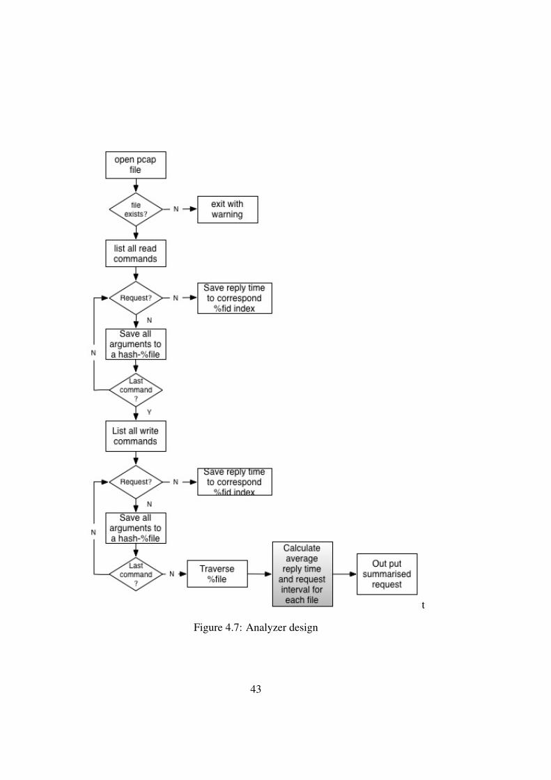
4.1 Design work flow for evaluation system[8] . . . . . . . . . . . . . 394.2 Learning system . . . . . . . . . . . . . . . . . . . . . . . . . . . 404.3 simulation system . . . . . . . . . . . . . . . . . . . . . . . . . . 404.4 Comparison system . . . . . . . . . . . . . . . . . . . . . . . . . 404.5 Design work flow for benchmark system[8] . . . . . . . . . . . . 414.6 Comparison system . . . . . . . . . . . . . . . . . . . . . . . . . 424.7 Analyzer design . . . . . . . . . . . . . . . . . . . . . . . . . . . 434.8 Fid structure . . . . . . . . . . . . . . . . . . . . . . . . . . . . . 444.9 Worker process . . . . . . . . . . . . . . . . . . . . . . . . . . . 484.10 Reply time collect . . . . . . . . . . . . . . . . . . . . . . . . . 49
5.1 Offset initial position histogram . . . . . . . . . . . . . . . . . . 535.2 Inter-arrival time for copy files . . . . . . . . . . . . . . . . . . . 545.3 Inter-arrival time for copy files zoom in . . . . . . . . . . . . . . 545.4 Histogram of inter-arrival time . . . . . . . . . . . . . . . . . . . 555.5 Offset initial position histogram . . . . . . . . . . . . . . . . . . 575.6 Inter-arrival time for copy files, red line stands for synthetic work-
load,the black line for original workload . . . . . . . . . . . . . . 585.7 Histogram of inter-arrival time . . . . . . . . . . . . . . . . . . . 595.8 Reply time . . . . . . . . . . . . . . . . . . . . . . . . . . . . . 61
6

List of Tables
3.1 Variables for Requests . . . . . . . . . . . . . . . . . . . . . . . 333.2 Variables for Responses . . . . . . . . . . . . . . . . . . . . . . 34
4.1 key parameters . . . . . . . . . . . . . . . . . . . . . . . . . . . 46
5.1 key parameters for original and synthetic workload . . . . . . . . 515.2 Request length for original and synthetic workload . . . . . . . . 555.3 key parameters for original and synthetic workload . . . . . . . . 565.4 Request length for original and synthetic workload . . . . . . . . 595.5 NAS server hardware information . . . . . . . . . . . . . . . . . 60
7

Chapter 1
Introduction
This chapter explains why we are focusing on storage benchmarking and whatchallenges we variety are facing?
1.1 MotivationAccording to the IDC report[9], world wide IT spending is expected to reach 2.14trillion dollars in 2014. The investment on storage reaches $37.3 billion by 2015.IDC also predicts that in the year of 2017, the raw digital data storage capacitycould rise to 7,235 EB. This tremendous amount of investment is great news forall the manufacturers in this industry, but it introduces new challenge as well.
Today we are in an information-explosion era, more and more companies cre-ate their private or public cloud environments. The enterprise storage system is acritical component of the entire system. The performance of the storage systemaffects all upper layer applications and devices.Realizing this fact, all the manufacturers advertise their storage system by per-formance specs. But the different products have been optimized for the differentdata structures and workloads. In some cases it is determined by the hardware,in other cases it is affected by manufacturers’ operation system on the top of theraw storage box. Hence there is not universal solution that can satisfy all kinds ofworkloads. The storage administrator has to conFigure a proper synthetic work-load carefully, which is demanding task for them.
Normally users always have one typical and common question for the pre-saleengineers, "I understand all the specs you have shown, but I am more interestedin how the performance will be in our product environment." Thus the best wayto answer the question is testing all target storages under real workload. It re-quires two steps. First one has to implement all target storages in their productenvironment, then create a mirror or snapshot of all their production data from the
8

original storage to the new target. By monitoring the performance matrix of thenew implemented storage system, one could make a solid conclusion about eachcandidate system. But in real cases, no company would do this, since the proce-dure requires a too large amount of human resource, time, financial support, etc.An alternative solution is naturally required. How one can test all target systemswithout affecting the product environment is very important.Some research has been done addressing this practical problem [2, 1, 3]. The ba-sic idea is so called Trace and Replay by [1]. The first step is to learn from thecurrent workload, and then create a synthetic workload based on what one learnedpreviously. According to [3], they have implemented a benchmarking tool, knownas TBBT, for NFS workload. They also applied with the trace and replay method-ology. There is also an solution for iSCSI protocol, developed by [2]. But there isnot any trace and replay benchmarking tool for SMB/CIFS protocol.
The thesis is to target this empty area. Our solution makes a methodologywithout full application deployment and which does not affect the performanceof the real production environment. This paper is focusing on SMB/CIFS storageprotocol environment, it is the most common storage protocol used in Windowsand Linux environment. By sniffing the network, one can trace storage transec-tions, and reproduce the workload based on it. The system can serves as a decisionmaking tool for storage administrator when purchasing.
1.2 Problem StatementTo get a more accurate benchmark result for every unique SMB/CIFS storageenvironment, we should learn from each environment and then generate the testworkload based on it. In this thesis, we focus on SMB/CIFS storage system in-stead of the local disk or storage area network (SAN) system. The reason forbypassing SAN/IP-SAN is that one has to implement an initiator to do that. Un-like the file level request replaying, one has to implement a client or an initiator forthe block level replay. This would require a long period of development. The timeis limited for this thesis work, so we only focus on SMB/CIFS benchmarking.
To accomplish our goal, we implement a system which solves the followingchallenges,
• How to learn the original workload without compromising users’ storageperformance
• How to generate a synthetic workload based on the first step
• How to show that the synthetic workload has the same impact as the originalworkload
9

• Run the simulation against different storage systems and verify that the re-sults are useful when evaluating the capacity of the storage system
By answering these three questions, we can show that our system is reliable tobenchmark the performance of a new SMB/CIFS storage.
10

Chapter 2
Background
In this chapter, we introduced all related knowledge. They include all storagestructures, benchmarking methodologies and related works.
2.1 Storage structuresToday, modern storage system is divided into three parts, DAS (Direct-AttachedStorage), SAN (Storage Area Network) and NAS (Network Attached Storage).The following sections introduce each of them respectively
2.1.1 DASDAS is most widely used in our daily life. It is a storage system directly attachedto a computer. It is a non-networked storage. Typically all hard disks connect toa server or a workstation through HBA (Host Bus Adapter). Since the structureof DAS does not rely on the network, and usually HBA is embedded in computer,DAS turns to be easy to use.
2.1.2 SAN2.1.2.1 History
Along with the data burst era came, DAS can no longer satisfy users’ requirementson capacity and performance. SAN is designed under such circumstance, whichintroduces the idea of separating storage system from computer system. SAN isdefined by Storage Networking Industry Association (SNIA) as a network. Its ma-jor mission is to transfer data among computer systems under high performance[4].
11

The most common protocol used by SAN is SCSI (Small Computer SystemInterface). In the early era of internet, SCSI protocol was designed for faster dataprocessing. This protocol is still commonly used in DAS structures today. SCSI isrecognized by its high performance and stability. Since most SAN are connectedthrough fiber channel, SCSI commands are transported over FCP (Fiber ChannelProtocol). SAN storage meets requirements on large scale storage capacity andhigh performance.
Although SAN has dominate advantages on capacity and performance, it isonly used in large companies or government at first. The reason is the pricesof fiber channel switch and cable are expensive compare to the Ethernet. Byrealizing the price is the major limitation of development in SAN technology,iSCSI (Internet Small Computer System Interface) protocol is innovated. Insteadof transferring SCSI command over FCP, iSCSI, known as IP SAN, are transferredby IP protocol through Ethernet network. IP SAN solution has the same structureas traditional FC SAN. The transfer speed of FC is 8 Gb/sec. It is higher thanEthernet cable with 1 Gb/sec. But the speed of new Ethernet is about to leapfrogfiber, with 10Gb/sec. In conclusion, IP SAN can run in the same speed as standardSAN storage. Meanwhile one can leverage from current enterprise IP network. Itlower the TCO (total cost of ownership) by sharing the existing IP network andnetwork administrators. More and more enterprises are migrating from FC SANto IP SAN recently.
2.1.2.2 SCSI
SCSI is a set of ANSI(American National Standards Institute) standard electronicinterfaces that used for system communicate with hard disks, tape drivers, CD-ROM drivers or printers.
SCSI commands are transferred in CDB (Command Descriptor Block). EachCDB can be a total of 6, 10, 12, or 16 bytes, but later versions of the SCSI standardalso allow for variable-length CDBs. The CDB consists of a one byte operationcode followed by some command-specific parameters.
There are two parts of SCSI architecture, clients and server. Client is definedas initiator in this module as server is target. Initiator will initiate any commu-nications between two parts. The target devices accessed by initiator, it uses asblock devices. A block device is a computer data storage device that supportsreading and writing data in fixed-size blocks, sectors, or clusters. This also meansthe file structure is transparent to SCSI devices. They need to break down a fileto blocks. So the host of initiators has the responsibility to mange how files arestored and retrieved. In the other word SAN devices only provided storage but notfile system.
12

2.1.2.3 iSCSI and IP SAN
The iSCSI protocol maps the SCSI to TCP/IP. It defines the way that how couldinitiator encapsulate the SCSI data to TCP/IP packet, and also how should targetdecode the coming TCP/IP packet to SCSI command and data. The benefits ofiSCSI protocol can be obviously, SCSI is the most common applied protocol bymost storages, tapes and other devices. Meanwhile TCP/IP is also the most stableand widely used network communication protocol. The combination of the twoprotocols makes iSCSI been an cheaper alternative solution of FC SAN.
2.1.3 NAS
Compare with SAN, NAS provides both filesystem and storage to clients. NASdevices will contain file system their self, which is totally isolated with the filesys-tem of clients. The architecture of NAS is also a client-server structure. Clientsuse particular protocol to communicate with server, the most widely used NASprotocols are NFS (Network File System) and SMB/CIFS(Server Message Block-/Common Internet File System). Both predate the modern NAS by many years;original work on these protocols took place in the 1980s. NAS is a remote fileprotocol. By definition, it must be accessed from remote devices through a cer-tain network, for example LAN. CIFS and NFS are also encapsulated by TCP/IPor UDP. That means NAS device can leverage from the current network environ-ments. NAS devices have their own IP address over network, so all users couldaccess to all files on NAS devices directly as long as their have the privilege to dosuch operation.
By setting up the file system on storage sides, the NAS devices could providemore file level function then SAN devices, for example user privilege control. Themajor task of NAS is how to find and mange files, instead of file itself, so this is adifferent scenario compare with block device such as SAN. This will be a criticaladvantage in enterprise environment, since they usually have very complicatedprivilege structure. NAS could employe the current user administration system,for example Active Directory for privilege control. The storage administrator willbe relieved from user management requirements. In the following sections, wewill introduce more details about NFS and SMB.
2.1.4 NFS
There are four versions of NFS since the first time it has been introduced by Sun.The most recently version of it is NFS V4. In this paper we will only discussabout version 4.
13
Figure 2.1: NFS history[5]
NFS is the first network file system. It began in the early 1980s as an experi-mental file system at Sun Microsystems. Since NFS protocol was widely used, itwas documented as a Request for Comments (RFC) specification. That was thetime NFSv2 was introduced. It evolved into version 3, by large file supporting,asynchronous writes, also used TCP as the transport protocol, which enabled itto extend to world wide network. Today, the newest version is 4.1, documentedas RFC 5661. The major change is they add protocol support for parallel ac-cess across distributed servers. IBM illustrated the history of NFS as Figure 2.2shows.2.1
NFS is a client-server structure, as Figure 2.3 shows [11]. It encapsulatesNFS CMD into TCP/IP packet. By capture the network transections, one canlearn attributes of files on serve, such as file name, path. NFS is also a statelessprotocol. File server does not store client information, and server and client donot maintain a connections between them. For example, NFS has no operation toopen a file, since this would require the server to store state information. Instead,NFS supports a Lookup procedure, which converts a filename into a file handle.This file handle is an unique, immutable identifier, usually an i-node number, ordisk block address. NFS does have a Read procedure, but the client must specifya file handle and starting offset for every call to Read. Two identical calls to Readwill yield the exact same results. If the client wants to read further in the file, itmust call Read with a larger offset.
2.1.5 SMB/CIFS2.1.5.1 History
SMB stands for Server Message Block, and CIFS stands for Common InternetFile System.
From CIFS to SMB version1 and SMB version 2, they have evolved SMBprotocol. They are developed by many of storage vendors and operating systemvendors for NAS solution. The first invention of SMB is by Dr. Barry Feigenbau,an IBM employee[6]. He first named it after his own name initial “BAF”, and then
14
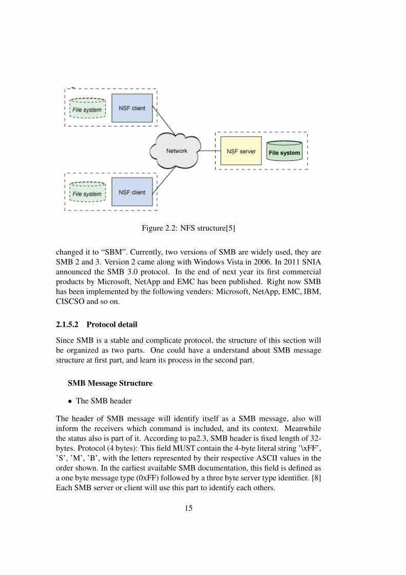
Figure 2.2: NFS structure[5]
changed it to “SBM”. Currently, two versions of SMB are widely used, they areSMB 2 and 3. Version 2 came along with Windows Vista in 2006. In 2011 SNIAannounced the SMB 3.0 protocol. In the end of next year its first commercialproducts by Microsoft, NetApp and EMC has been published. Right now SMBhas been implemented by the following venders: Microsoft, NetApp, EMC, IBM,CISCSO and so on.
2.1.5.2 Protocol detail
Since SMB is a stable and complicate protocol, the structure of this section willbe organized as two parts. One could have a understand about SMB messagestructure at first part, and learn its process in the second part.
SMB Message Structure
• The SMB header
The header of SMB message will identify itself as a SMB message, also willinform the receivers which command is included, and its context. Meanwhilethe status also is part of it. According to pa2.3, SMB header is fixed length of 32-bytes. Protocol (4 bytes): This field MUST contain the 4-byte literal string ’\xFF’,’S’, ’M’, ’B’, with the letters represented by their respective ASCII values in theorder shown. In the earliest available SMB documentation, this field is defined asa one byte message type (0xFF) followed by a three byte server type identifier. [8]Each SMB server or client will use this part to identify each others.
15

Command sector is a 8-bytes length structure. In the last version of SMB,version 3, there are 26 current used commands[8], we will discuss their details inlater section.
There are two kinds of flags. The first one of them indicates different featuresin effect for the message. Flags2 is a 16-bit field of 1-bit flags that represent var-ious features in effect for the message. Unspecified bits are reserved and MUSTbe zero.[8]
Tree ID (TID): The TID is a 16-bit number that identifies which resource(disk share or printer, typically) this particular CIFS packet is referring to. Whenpackets are exchanged which do not have anything to do with a resource, thisnumber is meaningless and ignored.
If a client wishes to gain access to a resource, the client sends a CIFS packetwith the command field set to SMB_COM_TREE_CONNECT_ANDX. In thispacket, the share or printer name is specified (i.e. \\SERVER\DIR). The serverthen verifies that the resource exists and the client has access, then sends back aresponse indicating success. In this response packet, the server will set the TIDto any number that it pleases. From then on, if the client wishes to make requestsspecific to that resource, it will set the TID to the number it was given.
Process ID (PID): The PID is a 16-bit number that identifies which processis issuing the CIFS request on the client. The server uses this number to checkfor concurrency issues (typically to guarantee that files will not be corrupted bycompeting client processes).
User ID (UID): The UID is 16-bit number that identifies the user who is is-suing CIFS requests on the client side. The client must obtain the UID from theserver by sending a CIFS session setup request containing a username and a pass-word. Upon verifying the username/password, the server responds to the sessionsetup and includes a generated UID. The client then uses the assigned UID inall future CIFS requests. If any of these client requests require file/printer per-missions to be checked, the server will verify that the UID in the request has thenecessary permissions to perform the operation.
A UID is valid only for the given NetBIOS session. Other sessions couldpotentially be using an identical UID that the server correlates with a differentuser. Note: if a server is operating in share level security mode (see above), theUID is meaningless and ignored.
Multiplex ID (MID): The MID is a 16-bit value that is used to allow multipleoutstanding client requests to exist without confusion. Whenever a client sends aCIFS packet, it checks to see if it has any other unanswered requests pending. Ifit does, it insures that the new request will have a different MID then the previ-ously outstanding requests. Whenever a server replies to a CIFS request, it insuresthat the response it sends matches the request MID that it received. In followingthis procedure, the client can always know exactly which outstanding request an
16

Figure 2.3: SMB header[8]
Figure 2.4: SMB parameter[8]
incoming reply is correlated to.
• The SMB parameter block
SMB was originally designed as a rudimentary remote procedure call protocol,and the parameter block was defined as an array of "one word (two byte) fieldscontaining SMB command dependent parameters". In the CIFS dialect, how-ever, the SMB_Parameters.Words array can contain any arbitrary structure. Theformat of the SMB_Parameters.Words structure is defined individually for eachcommand message. The size of the Words array is still measured as a count ofbyte pairs. The general format of the parameter block is as follows. 2.4
WordCount and parameter words: CIFS packets use these two fields to holdcommand-specific data. The CIFS packet header template above cannot hold ev-ery possible data type for every possible CIFS packet. To remedy this, the param-eter words field was created with a variable length. The wordcount specifies howmany 16-bit words the parameter words field will actually contain. In this way,each CIFS packet can adjust to the size needed to carry its own command-specificdata.
The wordcount for each packet type is typically constant and defined in theCIFS1.0 draft. There are two wordcounts defined for every single command; onewordcount for the client request and another for the server response. Two counts
17
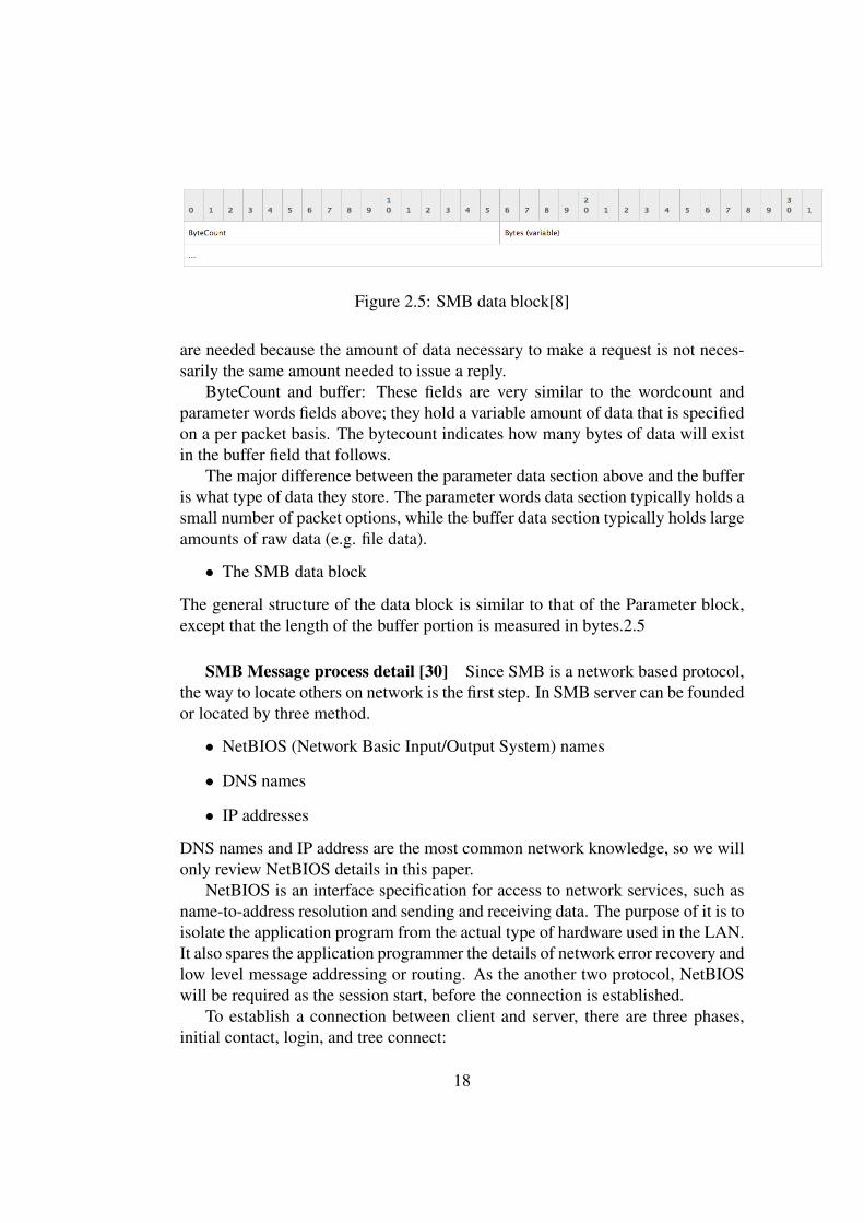
Figure 2.5: SMB data block[8]
are needed because the amount of data necessary to make a request is not neces-sarily the same amount needed to issue a reply.
ByteCount and buffer: These fields are very similar to the wordcount andparameter words fields above; they hold a variable amount of data that is specifiedon a per packet basis. The bytecount indicates how many bytes of data will existin the buffer field that follows.
The major difference between the parameter data section above and the bufferis what type of data they store. The parameter words data section typically holds asmall number of packet options, while the buffer data section typically holds largeamounts of raw data (e.g. file data).
• The SMB data block
The general structure of the data block is similar to that of the Parameter block,except that the length of the buffer portion is measured in bytes.2.5
SMB Message process detail [30] Since SMB is a network based protocol,the way to locate others on network is the first step. In SMB server can be foundedor located by three method.
• NetBIOS (Network Basic Input/Output System) names
• DNS names
• IP addresses
DNS names and IP address are the most common network knowledge, so we willonly review NetBIOS details in this paper.
NetBIOS is an interface specification for access to network services, such asname-to-address resolution and sending and receiving data. The purpose of it is toisolate the application program from the actual type of hardware used in the LAN.It also spares the application programmer the details of network error recovery andlow level message addressing or routing. As the another two protocol, NetBIOSwill be required as the session start, before the connection is established.
To establish a connection between client and server, there are three phases,initial contact, login, and tree connect:
18

When a CIFS client try to access resources on a CIFS server, it will process thefollowing packets in sequence. The NetBIOS session is established at first in orderto provide a reliable message sequence transport service. Then, the client andserver negotiate the CIFS dialect in which version they will use. The client then tryto login to the server, sending its username and password. Then if server verifiedthe coming user has the rights to access this shared storage, then the connection isestablished.
Packet #1 request, client –⌘ server Command id: SMB_COM_NEGOTIATE.Purpose: Establish NetBIOS session Summary: The client, wishing to exchangeCIFS packets with the server, initiates a NetBIOS session between itself and theserver (referred to as “calling the server” in the previous NetBIOS section). Thisprovides for sequenced, reliable message delivery between the two endpoints.Note that the client must know the server’s NetBIOS name in order to call it andalso must indicate its own NetBIOS name.
The events to establish the NetBIOS session are as follows. First, the clientestablishes a full duplex TCP connection with the server on port 139. Once this isaccomplished, the client builds and sends a NetBIOS session request packet (notdiagrammed in the NetBIOS section above, but described in RFC1002) over theTCP connection. In summary, the session request packet contains the client’s Net-BIOS name, the server’s NetBIOS name, and an integer constant which indicatesthe packet’s purpose is to establish a NetBIOS session. Please see RFC1002 formore details.
Packet #2 response, server –⌘ client Purpose: Positive NetBIOS session ac-knowledgement Summary: If the above session request packet contained the server’sNetBIOS name, and the packet was formatted correctly, the server replies with asimple session established acknowledgement. This 4-byte packet is also describedin RFC1002. In summary, it indicates either a successful session establishment oran error code.
Packet #3 request, client –⌘ server Purpose: Negotiate CIFS dialect Sum-mary: Now that the NetBIOS session is established, the client is ready to sendthe first real CIFS request. The client sends the SMB_COM_NEGOTIATE com-mand and includes a list of CIFS dialects that it understands. Packet: Command:SMB_COM_NEGOTIATE (0x72) TID: Ignored in this packet. PID: Set to pro-cess ID of client process. UID: Ignored in this packet. MID: Any unique num-ber. WordCount: 0 ParameterWords: There are none because wordcount is 0.Bytecount: Set to 119 (variable depending on how many CIFS dialects the clientunderstands). Buffer: Contains 119 bytes worth of dialect descriptions, exam-ples would be as follows: “PC NETWORK PROGRAM 1.0”, “MICROSOFTNETWORKS 3.0”, “DOS LM1.2X002”, “DOS LANMAN2.1”, “Windows forWorkgroups 3.1a”, “NT LM 0.12”.
19

Packet #4 response, server –⌘ client Purpose: Choose CIFS dialect from re-quest list Summary: The server is now responding to the negotiate protocol re-quest by selecting the dialect that it wishes to communicate in. Packet: Com-mand: SMB_COM_NEGOTIATE (0x72) TID: Ignored in this packet. PID: Ig-nored when packet is from server. UID: Ignored in this packet. MID: matchesunique number chose above. WordCount: This number depends on the dialectthat is chosen. For this example, we will assume that the server chose “NT LM0.12” [8] . In this case, the wordcount is 17. ParameterWords: The 17 wordscontained here indicate the chosen dialect and many server properties. Of note isthe MaxMpxCount (which states the max number of pending requests the clientcan initiate) and the 32-bit capabilities flags (which indicate if UNICODE is sup-ported, if large files are supported, if NT commands are supported, and more).Bytecount: Variable, usually greater than 8. Buffer: Typically contains an 8-byterandom string that the client uses in the next packet for encryption purposes.
Packet #5 request, client –⌘ server Purpose: User login Summary: Now thatthe CIFS dialect has been agreed upon, the client sends a packet containing ausername and password to gain a user ID (UID). This packet also relays clientcapabilities to the server, so the packet must be sent even if the server is usingshare level security. Packet: Command: SMB_COM_SESSION_SETUP_ANDX(0x73) TID: Ignored in this packet. PID: Set to process ID of client process. UID:Ignored in this packet. MID: Any unique number. WordCount: 12 Parameter-Words: This section is very similar to the server’s negotiate protocol parameterwords response. However, instead of listing the server’s capabilities, it lists theclient’s. It also contains the size of the passwords to be supplied in the buffersection below. Bytecount: Variable, the buffer below contains the encrypted pass-word, the username, the name of the operating system and the native LAN manger.Therefore, the size listed here depends on the string sizes of all these entities.Buffer: As mentioned above, this field actually contains the password, username,and other strings that identify the operating system involved.
Packet #6 response, server –⌘ client Purpose: Indicates User ID (UID) orreturns error if bad password Summary: Once the server receives the encryptedpassword and username, it checks if the combination is valid. If the password isinvalid, this response packet will be returned with the error class and code set tothe appropriate error value. If the username/password is correct, then this packetcontains the UID that the client will begin to send with every packet from hereon. Packet: Command: SMB_COM_SESSION_SETUP_ANDX (0x73) TID: Ig-nored in this packet. PID: Ignored when packet is from server. UID: The 16-bit number that the server has assigned to represent client user identity. MID:Matches unique number chose above. WordCount: 3 ParameterWords: Noth-ing relevant to normal operation. Bytecount: Variable, the buffer below containsstrings stating the server OS and native LAN manager type. Buffer: Contains
20

strings indicating the server OS and LAN manager type.Packet #7 request, client –⌘ server Purpose: Connect to particular resource
Summary: At this point, the client has authenticated itself to the server and mayproceed to connect to the actual share. In this packet, the client specifies theshare that it wishes to access. Share names are specified in UNC format (i.e.\\SERVER\SHARE). Packet: Command: SMB_COM_TREE_CONNECT_ANDX(0x75) TID: Ignored in this packet. PID: Set to process ID of client process. UID:Set to the server returned UID from the above session setup response. MID: Anyunique number. WordCount: 4 ParameterWords: Nothing relevant to normal oper-ation. Bytecount: Variable, depends on the size of the UNC string that is requestedbelow. Buffer: Contains the share name that the client wishes to access.
Packet #8 response, server –⌘ client Purpose: Indicates Tree ID (TID) or er-ror if share name does not exist Summary: If the share specified above existsand the user has access permission, then the server returns a successful responsewith the TID set to the number it wishes to refer to the resource as. If the sharedoes not exist or the user does not have access permission, the server will re-turn the appropriate error class and error code here. Assuming that this packetindicates success, the client now has everything it needs to access files from thespecified share. This is the final packet in this client/server exchange. Packet:Command: SMB_COM_SESSION_SETUP_ANDX (0x73) TID: 16-bit numberwhich server has assigned to represent the requested resource. PID: Ignored whenpacket is from server. UID: 16-bit number representing the user. MID: Matchesunique number chosen above. WordCount: 3 ParameterWords: Nothing relevantto normal operation. Bytecount: Variable, the buffer below contains strings statingthe native file system and device type of the requested resource. Buffer: Containsstrings that state the native file system and device type.
Then it is the process of file open and read.Once a client has completed the initial packet exchange sequence described
above, it may open and read files from the share that was requested. The fileopen consists of one CIFS request and one CIFS response. The read request alsoconsists of one request and one response packet.
Packet #1 request, client –⌘ server Purpose: Open a file Summary: In orderto read or write to a file, it first must be opened. This CIFS packet does exactlythat. Packet: Command: SMB_COM_OPEN_ANDX (0x2D) TID: Set to theserver returned TID from the tree connect response above. PID: Set to processID of client process. UID: Set to the server returned UID from the session setupresponse above. MID: Any unique number. WordCount: 15 ParameterWords:Specifies many open options such as mode (read, write, or readwrite) and sharingmode (none, read, write). Bytecount: Variable, depends on the size of the stringthat contains the filename. Buffer: Contains the name of the file to be opened.
21

Packet #2 response, server –⌘ client Purpose: Indicate File ID, or error code ifproblem Summary: The server checks to see if the filename above exists and if theuser specified in the UID has permission to access the file. If these conditions arenot met, the server will return the appropriate error class and error code indicatingwhat that problem is. If there are no errors, the server returns a response packetthat includes a File ID (FID) that can be used in subsequent packets for accessingthe file. Note that the FID is returned to the client in the parameter words field ofthe response. There is no FID field in the standard CIFS header. Packet: Com-mand: SMB_COM_OPEN_ANDX (0x2D) TID: 16-bit number which the serverassigned to represent the requested resource. PID: Ignored when packet is fromthe server. UID: 16-bit number representing the user. MID: Matches unique num-ber chosen above. WordCount: 15 ParameterWords: Many flags indicating whattype of actions occurred and the very important 16-bit FID. Bytecount: 0 Buffer:No data in buffer.
Packet #3 request, client –⌘ server Purpose: Read from a file Summary: As-suming that the above response indicated a FID for the client to use, an actual readrequest for file data can now be issued. Packet: Command: SMB_COM_READ_ANDX(0x2E) TID: Set to the server-returned TID from the tree connect response above.PID: Set to process ID of client process. UID: Set to the server-returned UID fromthe session setup response above. MID: Any unique number. WordCount: 10 Pa-rameterWords: Here, the FID is stated so the server knows which opened file theclient is referring to. Also indicated here are a 32-bit file offset and a 16-bit countvalue. These two numbers dictate where and how much data to return from thefile. Bytecount: 0 Buffer: No data in buffer.
Packet #4 response, server –⌘ client Purpose: Returns file data requestedSummary: This packet contains the requested file data. Assuming the UID,TID, and FID were all valid numbers in the request, an error here should be un-likely. Packet: Command: SMB_COM_READ_ANDX (0x2E) TID: 16-bit num-ber which server has assigned to represent the requested resource. PID: Ignoredwhen packet is from the server. UID: 16-bit number representing the user. MID:Matches unique number chosen above. WordCount: 12 ParameterWords: Here,the number of bytes that were actually read is indicated. This does not necessar-ily match the number requested (in case the request exceeded the file boundary).Bytecount: Variable, the buffer holds the file data, so this number is also the num-ber of bytes that were actually read. Buffer: The file data requested.
Then it is the process of file open and write.Once a client has completed the initial packet exchange sequence described
above, it may open and write files from the share that was requested. The fileopen consists of one CIFS request and one CIFS response. The read request alsoconsists of one request and one response packet.
22

Packet #1 request, client –⌘ server Purpose: Open a file Summary: In orderto read or write to a file, it first must be opened. This CIFS packet does exactlythat. Packet: Command: SMB_COM_OPEN_ANDX (0x2D) TID: Set to theserver returned TID from the tree connect response above. PID: Set to processID of client process. UID: Set to the server returned UID from the session setupresponse above. MID: Any unique number. WordCount: 15 ParameterWords:Specifies many open options such as mode (read, write, or readwrite) and sharingmode (none, read, write). Bytecount: Variable, depends on the size of the stringthat contains the filename. Buffer: Contains the name of the file to be opened.
Packet #2 response, server –⌘ client Purpose: Indicate File ID, or error code ifproblem Summary: The server checks to see if the filename above exists and if theuser specified in the UID has permission to access the file. If these conditions arenot met, the server will return the appropriate error class and error code indicatingwhat that problem is. If there are no errors, the server returns a response packetthat includes a File ID (FID) that can be used in subsequent packets for accessingthe file. Note that the FID is returned to the client in the parameter words field ofthe response. There is no FID field in the standard CIFS header. Packet: Com-mand: SMB_COM_OPEN_ANDX (0x2D) TID: 16-bit number which the serverassigned to represent the requested resource. PID: Ignored when packet is fromthe server. UID: 16-bit number representing the user. MID: Matches unique num-ber chosen above. WordCount: 15 ParameterWords: Many flags indicating whattype of actions occurred and the very important 16-bit FID. Bytecount: 0 Buffer:No data in buffer.
Packet #3 request, client –⌘ server Purpose: Write to a file Summary: Thisrequest is used to write bytes to a regular file, a named pipe, or a directly accessibleI/O device such as a serial port (COM) or printer port (LPT). Packet: Command:SMB_COM_WRITE_ANDX (0x2F) TID: Set to the server-returned TID fromthe tree connect response above. PID: Set to process ID of client process. UID:Set to the server-returned UID from the session setup response above. MID: Anyunique number. If the client negotiates the NT LAN Manager dialect or later theclient SHOULD use the 14-parameter word version of the request, as this versionallows specification of 64-bit file offsets. This is the only write command thatsupports 64-bit file offsets.
Packet #4 response, server –⌘ client Purpose: Returns write result Summary:This packet contains the write result status. WordCount (1 byte): This field MUSTbe 0x06. The length in two-byte words of the remaining SMB_Parameters.AndXCommand(1 byte): The command code for the next SMB command in the packet. This valueMUST be set to 0xFF if there are no additional SMB command responses in theserver response packet. AndXReserved (1 byte): A reserved field. This MUSTbe set to 0x00 when this response is sent, and the client MUST ignore this field.AndXOffset (2 bytes): This field MUST be set to the offset in bytes from the start
23
of the SMB Header (section 2.2.3.1) to the start of the WordCount field in thenext SMB command response in this packet. This field is valid only if the AndX-Command field is not set to 0xFF. If AndXCommand is 0xFF, this field MUSTbe ignored by the client. Count (2 bytes): The number of bytes written to the file.Available (2 bytes): This field is valid when writing to named pipes or I/O devices.This field indicates the number of bytes remaining to be written after the requestedwrite was completed. If the client wrote to a disk file, this field MUST be set to0xFFFF.<63> Reserved (4 bytes): This field MUST be 0x00000000. ByteCount(2 bytes): This field MUST be 0x0000. No data is sent by this message.
2.2 BenchmarkingBenchmarking technology is widely used by all industries. For example, mobilemanufacturers will post their benchmarking scores for every new device they post.By reading those scores users or customers could evaluate their performance. Itapplies for storage system. Unlike a mobile phone, storage systems usually workunder huge pressures, accessed by multiple servers, and meanwhile storage sys-tem is the slowest components compare with CPU, memory. The same methodol-ogy applies for system permanence test.
2.2.1 Network benchmarkingIn his 1999 HotOS paper, Mogul insisted that benchmarks must predict absoluteperformance in a production environment, rather than simply focusing on quan-tified, repeatable results in a carefully constructed laboratory setting [10]. Oneshould generate synthetic workload based on the current environment. By ana-lyzing original workload module, tools could adjust itself to simulate the TCPand UDP packets. There are several systems apply trace and replay methodol-ogy, for example, TCPivo. They use tcpdump to catch the original workload, anduse TCPivo to reproduce the synthetic workload. The trace and replay skills theyuse in such system, that is very similar with the system we are using in SAMBAbenchmarking.
2.2.2 Storage benchmarkingAlthough many manufacturers offer SSD (Solid State Drive) for better perfor-mance, but since the price of it is almost ten times then traditional hard drive disk,so in most cases customers have to use HDD (Hard Drive Disk) as their primarystorage system. So the performance results will affect users’ finial decision a lot.
24

But it is not that easy to benchmark a target storage system. Because storage sys-tems are in the bottom layer of OS kernel. It will be affected by all up-layersfacts, such as kernel daemons, applications access patterns, properties of files.Some storage systems are optimized for one or more applications such as DB(DataBase), or video applications. So it is hard to generate a universal workload to testall target storages.By AVISHAY [1] there are three popular methods to evaluate a storage system,they are
• Macro-benchmarks.
• Trace-Based.
• Micro-benchmarks.
For macro-benchmarks, one would employee this method under general purpose.Which means the workload or pressure generate by this kind of tools will representstandard requirement. That usually will not suitable for one’s interest, becausemost time the real workload in their product environments are unique.
Micro-benchmark is a adjustment for macro-benchmark, it will change someconfigurations or embedded with different types of operations to highlight one ormore aspects in that one. This requires a solid understand of current environmentsin order to adjust a proper simulate by optimization all operations. But it is stillhard to say whether the two workloads, the synthetic workload and the originalworkload, are the same. One could always argue with some other aspects will alsoaffect the result in someway.
Trace-Based tools is divided benchmarking with two steps. The first one istrace. The tool will learn the current environment by some method at first. Thenreplay it according to the pattern we learned from the first step. By doing thesesteps, we could generate the simulation more accurate as original workload, mean-while the results are more reliable for anyone depends on them. But to achievethat goal, one need to solve two challenges, one is how to collect the trace, andhow to replay it efficiently.
There are two types of tracing. The first one is to capture system calls. One canlearn about application dependencies between file system operations. The secondtype of tracing is to capture NAS protocol packets from network. Compare withfirst type, the advantage of the second one is that, it will no affect or lower thesystem performance when running capture tools. But it is difficult for user toknow about application dependencies and application think time from networkcapture.
25

2.3 Related workIn the paper of AVISHAY’s[1], it surveyed 415 file system and benchmarks from106 papers. It introduces all the currently used benchmarking methodologies, andalso it argued how to present and discuss the test results. It categories the threekinds of benchmark system.
• Macrobenchmarks
• Trace Replays
• Microbenchmarks
Macrobenchmarks is that one test storage system against a particular workload.The workload can usually represent some real industrial workload. The advan-tage of this method is that it is good for overall view of the storage system andeasy to implement. But the tradeoff is that the result maybe not reliable, sincethe workload may not be realistic. Postmark[13, 14] is one of the most famousbenchmark tools in this category. SPEC (The Standard Performance EvaluationCorporation)[16], TPC (The Transaction Processing Performance Council)[15]and SPC (The Storage Performance Council)[17] are three organizations whichfocusing on macorbenchmarks tools and workloads development.
Microbenchmarks test the same storage system serval time, and modify a vari-able or some variables each time. So one can isolate the bottleneck from the sys-tem. Bonnie++[18] is a fairly well-known benchmark tool. It performs a seriestest on a single file. Based on the test, it reports the process capacity per secondfor CPU and the percent of CPU usage.
They defines the benchmark tools, in the “trace-based” category, as “A pro-gram replays operations which were recorded in a real scenario, with the hopethat it is representative of real-world workloads.” It is critical to generate an iden-tical synthetic workload of the original workload. Recent studies point out thatstorage workloads are diverse. They vary widely from different applications theyserve. Therefor how to measure a workload is important. This paper[1] is ourguid book for the entire system, since it listed all the key variables to evaluate astorage system by a benchmarking tool.
For all benchmarking systems belong to this category, they trace the workloadfirst and analyze the workload, at last step they generate the synthetic workloadbased on previous analyze results.
• Trace capture: There is no accepted way to capture traces. Traces can becaptured at the system call, networking, and driver levels.
– System call: It is easy and the system call API is portable[19, 20, 21],but the tradeoff is it adds extra work on the system.
26

– Network traffic: Specialized tools[22, 23] only work for network basedstorage protocol, and the trace file only contain requests that were notsatisfied from the cache.
– Driver level: Driver-level traces contain only non-cached requests. Butit is unable to correlate the requests with the associated meta-data[24].
• Replay: Some extra work is required before one can generate a syntheticworkload successfully, and replay method should be chosen carefully.
– Extra work
⇤ Target file system must be prepared.⇤ Missing operations have to be guessed[3].
– Replay method
⇤ Replay level: In the most common case, one should replay tracesat the level the traces were captured. Network replaying can bedone entirely from the user-level.
⇤ Replay speed: Many believes that the trace should be played asfast as possible[25, 26, 27, 28]. The timings of the original work-load should be ignored. But there are replaying tools, such asButtress[29] , that have been shown to follow timings accurately.
According to Christina et. [2], the workload pattern of block device can be identi-fied with Markov Chain module. They implemented the trace-based benchmark-ing tool for IP-SAN. In their model they used the Markov Chain to represent thecharacteristics of the original workload. Characteristics correspond to ranges oflogical blocks on disk (LBN). Transitions related to the probabilities of switchingbetween LBN ranges. Transition is characterized by block size, randomness, typeof IO and inter-arrival between subsequent request. The probabilities for transi-tions is calculated as the percentage of correspond I/Os. But they did not discussabout other type of storage system, they mainly introduced about SAN or IP SANstructure.
In the paper of Ningning[3], they also implemented their benchmark systemaccording to trace and replay methodology. They focused on NFS. They use thenetwork sniff to capture original workload. Then they create initial file systemimage according to the NFS trace. Their approach is similar compare with ours.Instead of benchmarking NFS system, we implement a SMB benchmark system.
27

Chapter 3
Method
This chapter will introduce the reader to the methods, tools and equipment usedin this project.
3.1 System modelAs explained in the introduction, one will need two subsystems to benchmark thetarget storage. First it requires to trace the current system workload.
The SMB/CIFS protocol transfers all information through network. We traceall network packets from different network structure. But a single point to pointnetwork structure is enough for us to evaluate our results and design.
The first subsystem is learning system. Two major components are involved init. The first part is product storage, which is responsible for the current productiondata access requirements. The second one is the learning system, with this system,one grabs the SAMBA/CIFS data flow by copying the TCP traffic flow from theport connected with storage. The port number for SAMBA/CIFS service is TCP445. It shows in Figure 3.1
The learning system is running a Ubuntu 13.04 server version. The systemwill use TCPDUMP to track the input and output traffic on product storage. Theoutput of the learning system is a pcap file. After data collection, the learningsystem will also response for generating a analyze report for previous collectedworkload, and an operation list. The goal of this step is that one can learn all thecharacteristics of the workload. As mentioned before, the key for generating arealistic synthetic workload is to trace the all characteristics of original one andreplay according to it.
We named the second system as simulation system, it will simulates the work-load based on the operation list, that is generated by learning system. We em-ployed the second system at two stage.
28

1. Under the different environments, one should evaluate our system first be-fore one can use it as a benchmarking system. We discussed the reason inChapter Discussion. The key to evaluate our system is to compare the syn-thetic workload with the original workload. The two workloads should havethe same characteristics. After all the informations of the original workloadare learned by learning system, a synthetic workload is going to be made. Atthis stage, the synthetic workload is used to test in the original environmentagain, which means we test the product storage with synthetic workload,and all network informations are captured in the same way by learning sys-tem. Then the two workloads are compared by their characteristics.
2. Once one has evaluated the system is capable to generate the similar work-load as the original one, then the system is used to benchmark the multipleNAS storage systems. In this stage, the synthetic workload is used to testmultiple target storage systems. Once the simulator start to generate thepressure for target storage, monitor will run again to dump the syntheticworkload. It shows in Figure 3.2. Unlike the previous step, the character-istics are identical for all the synthetic workloads, since we use exactly thesame workload for all targets. Then we only compare their reply times foreach NAS storage system. The reply times represent their performances.
3.2 Tools and equipmentOur system is developed in a virtual environment, and the network structure is apoint to point connection. But all of our tools are capable in larger and complicatorenvironment. We picked up the current system configuration according to ourresource and time limitations.
3.2.1 Workload traceTo trace the workload, one needs to use switch port forward technical on switch.Switch port forward technical is also known as port mirror, it is generally usedby networking troubleshooting. By setting up port mirroring on switch, one canreceive all packets on the port connected with storage. Most of modern switchdevices support this function. The port mirror feature was introduced on switchesbecause of a fundamental difference between switches and hubs. A hub broadcastsa packet to all ports whenever it receives it on one, but it will not send it to the onethat receives it. Instead of broadcasting packets among all ports, the switch willcreate a forwarding table on the physical layer, based on MAC address. Based on
29

Client PC
Client PC
Client PC
Client PC sniffer
Ethernet EthernetProduct storage
tcpdump
Figure 3.1: Learning system structure
sniffer
Ethernet EthernetTarget storage
tcpdump
simulator
Figure 3.2: Simulation system structure
30
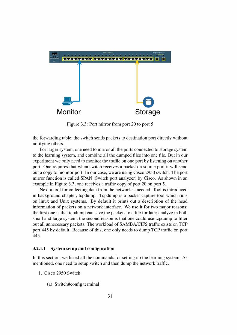
Figure 3.3: Port mirror from port 20 to port 5
the forwarding table, the switch sends packets to destination port directly withoutnotifying others.
For larger system, one need to mirror all the ports connected to storage systemto the learning system, and combine all the dumped files into one file. But in ourexperiment we only need to monitor the traffic on one port by listening on anotherport. One requires that when switch receives a packet on source port it will sendout a copy to monitor port. In our case, we are using Cisco 2950 switch. The portmirror function is called SPAN (Switch port analyzer) by Cisco. As shown in anexample in Figure 3.3, one receives a traffic copy of port 20 on port 5.
Next a tool for collecting data from the network is needed. Tool is introducedin background chapter, tcpdump. Tcpdump is a packet capture tool which runson linux and Unix systems. By default it prints out a description of the headinformation of packets on a network interface. We use it for two major reasons:the first one is that tcpdump can save the packets to a file for later analyze in bothsmall and large system, the second reason is that one could use tcpdump to filterout all unnecessary packets. The workload of SAMBA/CIFS traffic exists on TCPport 445 by default. Because of this, one only needs to dump TCP traffic on port445.
3.2.1.1 System setup and configuration
In this section, we listed all the commands for setting up the learning system. Asmentioned, one need to setup switch and then dump the network traffic.
1. Cisco 2950 Switch
(a) Switch#config terminal
31

(b) Switch(config)#monitor session 1 source interface fastEthernet 0/25
(c) Switch(config)#monitor session 1 destination interface fastEthernet 0/5
2. Tcpdump
(a) root# tcpdump port 445 -w oringinalworkload.pcap
3.2.2 Capture file analyzeThe capture file is a standard pcap (packet capture) file. We use tshark to analyzethem. Tshark is known as text version of wireshark, which is one of the bestpacket analyzers. Tshark is similar with tcpdump but has some integrated sortingand filtering options. We take advantages from SMB filtering options of tshark.Tshark enable us to filter SMB traffic by SMB commands, and it offers a statisticresult of reply time for each correspond requests. In our system, we require onlywrite and read workload between server and clients. For each request we need toknow the timestamp for this packet, start offset, length for this request, Fid andfile name. One can collect all of those necessary information from tshark outputas ?? shows. Besides that we also require reply time for this request, the result ofreply time is used for later comparison.
One could specify the SMB command by “smb.cmd== ” options. As we listedin Introduction part, the command id for read is 0x2e, and it is 0x2f for writerequest. By extend normal tshark command with smb.cmd==0x2e(Read request)options, tshark generates the results as shown in following log. The output ofsmb.cmd==0x2f (Write request) is very similar with previous one, but it showsWrite AndX Request in command field. The log file is discrete log, it combinesboth read requests and write requests, and their replies. But this log can presentall the information we used in later phrase.
Log of tshark output:21461 53.761943 10.0.0.40 -> 10.0.0.2 SMB 117 Read AndX Request, FID: 0x2407, 61440
bytes at offset 14987264 smb.file == "\\a.rvt"21462 53.761969 10.0.0.40 -> 10.0.0.2 SMB 117 Read AndX Request, FID: 0x2407, 61440
bytes at offset 10854400 smb.file == "\\a.rvt"21463 53.761971 10.0.0.40 -> 10.0.0.2 SMB 117 Read AndX Request, FID: 0x2407, 61440
bytes at offset 12951552 smb.file == "\\a.rvt"21465 53.762280 10.0.0.2 -> 10.0.0.40 SMB 237 Read AndX Response, FID: 0x2407, 61440
bytes smb.time == 0.000337000 smb.file == "\\a.rvt"21480 53.764403 10.0.0.2 -> 10.0.0.40 SMB 237 Read AndX Response, FID: 0x2407, 61440
bytes smb.time == 0.002434000 smb.file == "\\a.rvt"21489 53.765769 10.0.0.2 -> 10.0.0.40 SMB 237 Read AndX Response, FID: 0x2407, 61440
bytes smb.time == 0.003798000 smb.file == "\\a.rvt"44047 92.872010 10.0.0.40 -> 10.0.0.2 SMB 1418 Write AndX Request, FID: 0x23d6, 65536
bytes at offset 208142336 smb.file == "\\a.rvt"
32

Column 1 Sequence number of the packet It indicates the order of the packetColumn 2 Time stamp of the packet Time stampColumn 3 Source and Destination The IP addresses of Server and ClientColumn 4 Operation type The request type of this packetColumn 5 FID A file handle, representing an open
file on the server.Column 6 Length Requested lengthColumn 7 Offset Offset of the requestColumn 8 Requested file File name
Table 3.1: Variables for Requests
44049 92.872060 10.0.0.40 -> 10.0.0.2 SMB 1418 Write AndX Request, FID: 0x23d6, 65536bytes at offset 208207872 smb.file == "\\a.rvt"
44051 92.872495 10.0.0.40 -> 10.0.0.2 SMB 64294 Write AndX Request, FID: 0x23d6,65536 bytes at offset 208273408 smb.file == "\\a.rvt"
44053 92.872716 10.0.0.2 -> 10.0.0.40 SMB 105 Write AndX Response, FID: 0x23d6, 65536bytes smb.time == 0.001794000 smb.file == "\\a.rvt"
44057 92.873066 10.0.0.2 -> 10.0.0.40 SMB 105 Write AndX Response, FID: 0x23d6, 65536bytes smb.time == 0.001056000 smb.file == "\\a.rvt"
44058 92.873170 10.0.0.2 -> 10.0.0.40 SMB 105 Write AndX Response, FID: 0x23d6, 65536bytes smb.time == 0.001110000 smb.file == "\\a.rvt"
We listed all the variables of requests in the Table 3.1. The time stamp is usedfor us to simulate the inter-arrival times between requests. Since in this thesis,we only simulate the situation of a point to point connected server and client, theaddresses of the destination and the source are dropped. The operation type isused to category all requests by their type. In later stage one need to call differentsubroutines for different types of operation. As one can see, a single file hasmultiple FIDs. The FID is representing an open file on server, in that case, themultiple FIDs for a single file means that the file is opened multiple times by aclient or different clients.
Most of the variables we get from the reply packet are the same as the requests.But the reply time is only observed in reply packet. We use the reply time toevaluate the performance of a storage system.
To store all the arguments from this step, we employ perl to go through allpackets of the pcap file. In our case, a pipe connects the tshark command outputand our scripts. A pipe is a unidirectional I/O channel that can forward a streamof bytes from one process to another. In that case, all outputs of tshark will beredirect as input to our script. Then we use perl REGEX (Regular expression)function to dispatch each output, and store them in to correspond variables.
The analyze script is response to generate two files. Result report is the firstone, it includes summarize of all statistic result of workload. It shows all details
33

Column 1 Sequence number of the packet It indicates the order of the packetColumn 2 Time stamp of the packet Time stampColumn 3 Source and Destination The IP addresses of Server and ClientColumn 4 Operation type The request type of this responseColumn 5 FID A file handle, representing an open
file on the server.Column 6 Length Replied lengthColumn 7 Requested file File nameColumn 8 Time The time between the response and its request
Table 3.2: Variables for Responses
of files that been accessed, which includes the average inter-arrival between eachaccess, the total request data length for each file, average response time for allrequests of each file. The analyze script generates an operation lists file as well.This file lists all requests and their arguments, for example timestamp for eachrequest, command type etc. It is prepared for simulation part.
3.2.2.1 System setup and configuration
The command we used to get the informations of the packets.
1. Tshark command
(a) For read request: sun@guang-ubuntu-server:~/code$ tshark -R "smb.cmd==0x2e"-r test3.copyeclipse.pcap
(b) For write request: sun@guang-ubuntu-server:~/code$ tshark -R "smb.cmd==0x2f"-r test3.copyeclipse.pcap
2. Perl pipe command
(a) open (r,"tshark -R ’smb.cmd==0x2e’ -z proto,colinfo,smb.file,smb.file-z proto,colinfo,smb.time,smb.time -r $f|");
3.2.3 SimulationIn this part, two tools is required. Linux “dd” command is used to generate all filesthat listed in operation. The “dd” command works for converting and copying afile. The reason for using dd copy function as a file generator in our system is that,by supplying appropriate arguments for dd, we can generate file with accurate size
34

Figure 3.4: Random read example
and random content. /dev/urandom is the source file for dd command. /dev/uran-dom is embedded by Linux as a character special file - it provides an interface tothe kernel’s random number generator.
In some case, a file is accessed randomly instead of sequentially. For example,as shown in 3.4, the file was read from three different start offset. To simulate itone should set start offset and length for each request. So a SAMBA client appli-cation is required to fulfill the requirements. We are using perl Filesys-SmbClientmodule. It is a interface for accessing Samba filesystem. One can simulate normalread and write access and move file offset of a file handler by calling this module.A request from Filesys-SmbClient module bypasses buffering, then the simula-tion operations can be spotted on network exactly the same as asked. This partis very important for simulator to generate a similar workload. Otherwise servaloperations might be ignored because of they stored already in cache by previousrequest.
3.2.3.1 Oplist
Oplist is generated at the last step of the learning system. It contains all the in-formation which are used by simulation system. As we mention in 3.2.2, thesimulator should be able to generate a similar workload according to the key char-acteristics. The first column indicates the operation type of the request, and thesecond column indicates the time of the request should be generated. The time iselapse time since the first packet. The third and fourth column present the startoffset and the length of the request. The last two column show the file information.The FID information is used to identify each open operations for a file. When wereplay the synthetic workload according to this oplist file, one can easily tell whenshould an open operation should be invoked according to different FID.
3.2.3.2 System setup or configuration
1. dd
(a) dd -if=/dev/urandom -of=/share-location-for-a-share/filename bs=filesizecount=1
2. Filesys-SmbClient
35

(a) Create SAMBA client instance: my $smb = new Filesys::SmbClient(username=> "", password => "", workgroup => "WORKGROUP");
(b) Open a file and save the file handle to a variable:
$a=$smb->open("smb://10.0.0.2/share2/eclipse/jre7/lib/fontconfig.properties.src");
(a) Sets FILEHANDLE’s system position in 0: $smb->seek($a,0);
(b) Attempts to read 2 bytes of data into variable $a from the specified filehandler $a: $smb->read($a,2);
36

Chapter 4
System design
In this chapter, we introduced the design of our system. We designed the systemfor two scenarios, the first is evaluation, the other is benchmarking. As mentionedin 3.1, our system has two major subsystems, learning system and simulation sys-tem. In this chapter we first explained the different approaches for the two scenar-ios and then we introduced the design and implement details for both subsystems.
4.1 Work flow introductionBy this tools, we intent to develop a light weight tools, which can both monitorthe current Environment and generate the synthetic workload based on previousworkload. According to Avishay ET.AL [1], they mentioned such method by"trace and replay", it is the method we are using in our system. The learningsubsystem is used to analyze the
4.1.1 EvaluationAs shown in Figure 4.1, we divided our system into 7 modules, they are listedon the left side of Figure 4.1. They work together to fulfill the requirement oftrace and replay benchmarking. The right side of Figure 4.1 is the outputs thatgenerated by each module.
At this point, our goal is to evaluate the synthetic workload. We use the keycharacteristics of different workloads to compare them. At first one should learnall the characteristics of the original workload, then a synthetic workload is gen-erated according to the informations of the original workload. Then we ran thesynthetic workload on the same product environment again and collected the net-work traffics. After we analyzed the network dump file of the synthetic workload,
37

we summarized all the characteristics of the two workloads, and compare them.Since both time we use the same storage system, so the difference of those twoworkloads are caused by our system only.
We use the first three subsystems to learn from original workload. They in-clude tracing function and an analyzer script. The learning system also generatethree files as output, they are a pcap file, operations list file and a result report.
Then a simulation system is involved in next step. It replays a synthetic work-load and it records the traffic information as learning system. Therefor its outputis also a pcap log file.
At the last part of our system, a sub system called comparison system is em-ployed, shown in Figure 4.4. It analyzes the capture file of simulator and generatea result report for synthetic workload. Then the system compares both reports oforiginal workload and simulation workload.
4.1.2 BenchmarkingAt this point, our goal is to benchmark different NAS storage systems with thesynthetic workload. We use the key characteristics of different workloads to com-pare them. At first one should learn all the characteristics of the original workload,then a synthetic workload is generated according to the informations of the orig-inal workload. The synthetic workload is used for all the NAS storage systems.Each time the network traffic is collected, and the mean value and standard devia-tion of the reply time are calculated according to each network dump file as shownin Figure 4.5.
As the evaluation, We use the first three subsystems to learn from originalworkload. One need to collect longer period traffic then evaluation stage.
Then we use the simulation workload to benchmark all the NAS systems. Itreplays a synthetic workload several times and it records the traffic information aslearning system. At the last part of our system, a sub system called comparisonsystem is employed, shown in Figure 4.4. It analyzes the capture file of simulatorand generate the mean value and the standard deviations of the reply times for eachtime test. The mean values of the reply times are used to evaluate the performanceof the target NAS storage systems.
4.2 Learning system designFirst we are focusing on trace part, in this part one critical mission is how to collectall the necessary information we need. After monitor the product environment fora while, we have to understand what are the workload characterizations. In caseto replay it more accurate, we generate the simulation R/W operation as original
38

Trace current workload from network layer
Analyse capture file
Generate all files on target storage
Running simulator to generate
synthetic workload
Analyse caputure file
Compare results report
Trace the workload from network layer
Workload pcap file
Operationlist
Resultreport
File structure as original file
system
Workload pcap file
Result report
Work flowOutputInput
System process Output list
Figure 4.1: Design work flow for evaluation system[8]
39

Trace current workload from network layer
Analyse capture file
Workload pcap file
Generate all files on target storage
Operation list
Result report
Learning system Output list
Out putIn put
Out put
In put
Figure 4.2: Learning system
Running simulation
workload with synthetic workload
Trace current workload from network layer
Workload pcap file
Simulation system Output list
Out put
Figure 4.3: simulation system
Analyse capture file
Compare results
Result report
Comparison system
Out put list
In put
Figure 4.4: Comparison system
40
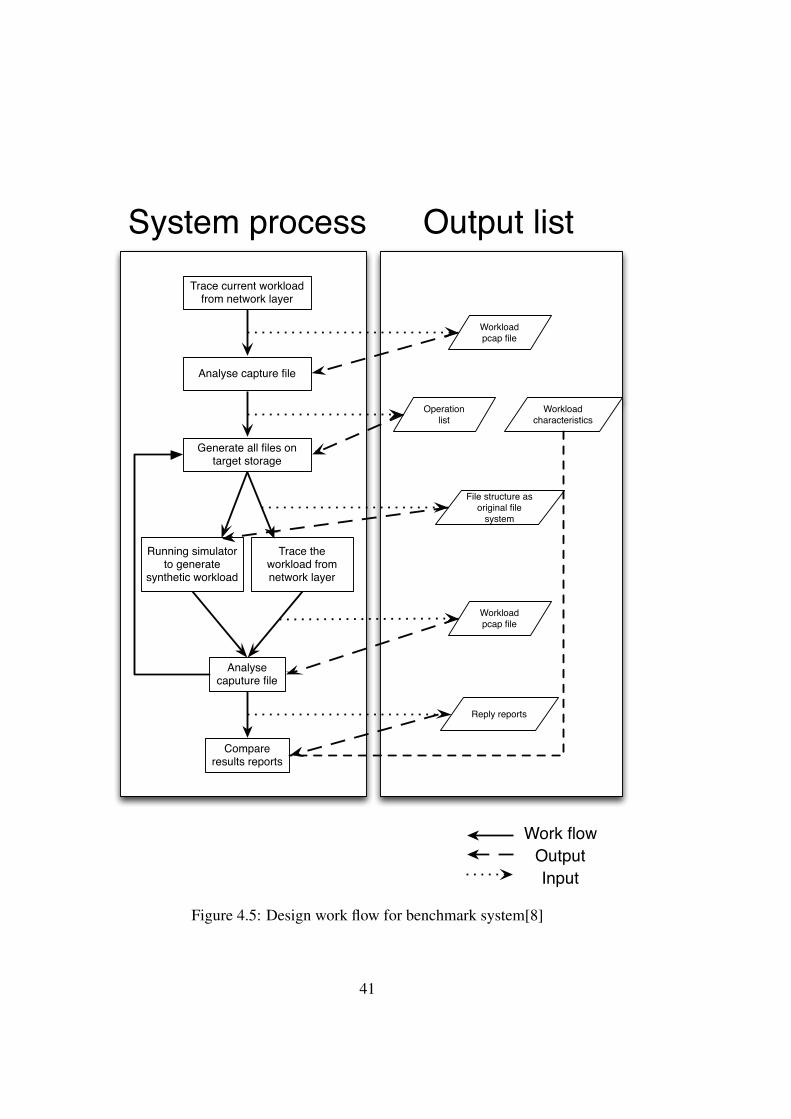
Trace current workload from network layer
Analyse capture file
Generate all files on target storage
Running simulator to generate
synthetic workload
Analyse caputure file
Compare results reports
Trace the workload from network layer
Workload pcap file
Operationlist
Workload characteristics
File structure as original file
system
Workload pcap file
Work flowOutputInput
System process Output list
Reply reports
Figure 4.5: Design work flow for benchmark system[8]
41

Analyse capture file
Compare results
Result report
Comparison system
Out put list
In put
Figure 4.6: Comparison system
ones, to do that it requires us to decode all operations and log them down for thenext step. Without it one is not able to prove whether the synthetic workload isidentical compare with the original workload. In the first part we need to do thefollowing tasks by developing the learning system.
4.2.1 Capture traffic information: The learning system willcollect current product SMB (Server Message Block) traf-fic information.
In this step, the implement is straight forward. One needs to dump the SAMBAtraffic to a pcap file.
4.2.2 Analyze log file which is dumped in previous stepAnalyzer is response for two outputs, the first one is a result report, the secondone is a operation list.
We designed the analyzer scripts as shown in Figure 4.54.7. After collected thetraffic dump file, we open this file and process it twice as showed. First the scriptfilter the pcap file with only read command traffic, which include both requestsreplies. The script break down each packet information, and save all requiredelements to a hash variable– %fid. The structure of %fid is a nested structure asshown in Figure 4.6. At the first level we use file name to index all entries.
The structure of %fid is a nested structure as shown in Figure 4.6. At the firstlevel we use file name to index all entries. We only save two types of commands,read and write, it serves as second level index, Then each file can be opened bydifferent processes concurrently, the SAMBA server assigns a unique fid to eachopen request for a file. After the first three level index, the script push all detail
42
t
Figure 4.7: Analyzer design
43

Figure 4.8: Fid structure
arguments of a command in to an array. We employees the array - hash structureto store all the details. We use the time stamp to calculate the time inter-arrivalbetween each requests, and we sum up the correspond sequential requests lengthand only present the start position and total length as one record in operation list.By integrating all sequential access requests as one record, one can achieve betterperformance in simulation system, without compromising the workload character-istic. Since we create any random offset access as separate records. According tothis structure of fid, one is also able to calculate how many times a file is opened,how many requests for each open fid and total length acquired for this file. Theinter-arrival time for each request of one open file handler is also been calculated.Since we only monitor the workload on network layer, so the application layerdependence relationship is transparent for us. Therefor the timestamp is a criticalelement to approach the similar parallel I/O pattern.
44

4.2.3 Identify workloadIt is critical for us to compare the simulation workload with the original workload.The result can verify the accuracy of our system. In this step, the key properties ofa workload are used to identify one. As mention by [12], the following argumentsare used to identify a workload:
• Total data length
• Total files
• Average file size
• Read requests
• Write requests
• Mean value of the length of the requests
• Standard deviation of the length of the requests
• inter-arrival time between requests
• offset distance of discrete requests
• Total read request length
• Total write request length
A workload can be defined by these arguments. In the evaluation stage, originalworkload and synthetic workload are used to test the same storage system twice,then calculate all the arguments for each time. By comparing them, one can tellwether the two workloads are similar or not.
4.2.4 Generate a workload report, which will represent all keycharacterizations by the previous workload identification
As one of the two outputs of this step, and according to Figure 4.5, the learningsystem represents a report which lists all key parameters for identifying a work-load. All these parameters are used for both evaluating new storage system andvalidation of current system. The output files are organized by files appeared innetwork trace.
45

Name ExampleRequest inter-arrival 5.23 e-15Request length 57890 BytesOperation type WReply time 0.0000434 sFrequency 23
Table 4.1: key parameters
4.2.5 Generating a synthetic workload operation list.Refer to 4.2.1, an operation list is created based on the request details. Instead ofwrite all request entries to oplist file, those sequential requests are integrated as asingle request with their first offset and their total length. In this file, requests areorganized as : operation type; time stamp; start offset; length; fid; file name.
4.3 simulation system designAfter data collection and analyzation step, we need to replay a synthetic workload.For any storage system, one will experience four kinds of operations, Write/Readoperations, and meta operations. We will only replay all read and write operationsby this tools, since they will generate the most pressure to storage system. Oursimulation system is divided into three parts. The first part is preparation part, itreads oplist file and store all requests parameters to a hash variable- %fid. Thethread pool is prepared in the preparation part. Using the thread pool can save oursimulator from thread create and reclaim. Since the one could only simulate theparallel workload according to time stamp, we need to shrink the overhead of thesimulator. Thread pool creates all worker threads as required, and each time a newthread is called, thread pool assigns a available worker to it. Then after the workfinishes its task, the thread pool reclaims it afterward.
The original workload is simulated based file level access pattern. The simu-lator open the target file at the exactly time as original workload did, then performall operations for this file handler sequentially. To do that the simulator requiresthe timestamp for opening a file, then the worker of the simulator is passed allrelated arguments for replay actual read or write operations.
Each time the worker receives the following arguments:
• File name
• Operation type
• Operation start offset list under an unique file handler
46

• Operation length list under an unique file handler
A worker open a file according to the file name, and then set the offset one byone according to the offset array. Each time after the worker set up the offset, itstart to perform a read or write operation as the arguments specified. All opera-tions for the same file will be performed linearly. The reason for that discussedin Chapter 7 Conclusion. The Figure 4.74.9 shows the simulator will continues toperform the read or write operation according to the operation list, until it traverseall the elements in the operation start offset list, which is passed as an argumentfor worker. The file handler is closed at the bottom of the worker to avoid ex-ceeding of the limitation of operation system. Because it is a linearly process ina single thread, so we can make sure the access sequential is exactly the same asthe original workload.
Simulator begin to generate the synthetic workload as shown. Meanwhile oneexecutes the monitor on network again to capture all information for syntheticworkload. The learning tool is used again for two reasons:
• Compare with original workload to calculate accuracy rate.
• Compare with test results of other test target storages to evaluate them.
4.4 Comparison system designTo compare the results between the different storage systems, we need to recordtheir reply time for each response. Tshark is used to collect the reply time from thelog file. Tshark can extended its function with a parameter “-z” to display the ex-tra information of each packet. We use the “-z proto,colinfo,smb.time,smb.time”to show the time inter-arrival between a response packet and the related requestpacket. In Figure 4.10, we listed the work flow of this part. As shown, the replytime is only revealed inside response packet. After we log the reply time into afile named replytime.csv, we can compare this file with others’ replytime.csv. Themean value and standard divination can be calculated later.
47

Open a file according to operation type
Save the file handler to a variable
Read from the offset list to get the start offset
Set the offset to the previous locate position
Read from the length list to get the length for read or write operation
Read or write
Is this the last operation?
N
Close file and exit thread
Y
Figure 4.9: Worker process
48

open TCPdump
log file
file exists?
Is it a response package?
Log the response
time to replytime.csv
Figure 4.10: Reply time collect
49

Chapter 5
Results
This chapter describes the experiments and their results. The result and systemdesign is divided into two chapters. The chapter 4 shows all the design process andmakes a clear separation between results and the incremental experiment design,the design considerations were put in the separate system design chapter. In thischapter we organized the results in three parts, They are analyze report for originalworkload, analyze report for synthetic workload, and the compression report forthem. The first one and the second one listed the result for evaluation our systemin different environments, which is explained in Section 4.1.1. The last part listedthe result for benchmarking, one can find the related design in Section 4.1.2.
We use a the4.1 to identify the workload. We have run our tests with differentworkloads.
5.1 Copy file workloadAs we mentioned in previous chapters, the original workload is the workload wedumped in the product environment. The synthetic is the workload we generatedby the simulation subsystem.
The first experiment is performed using the following setup:
1. Windows 2008 server as client
2. Ubuntu 12.04 64 server as SAMBA server
3. Direct connection between the client and server
4. The original workload is to copy 13 pictures from the SAMBA server to thelocal disk of the client
50

Original workload Synthetic workloadTotal data length 11620313 byte Total data length 11620313 byteTotal files 13 Total files 13Average file size 893870.2 Average file size 893870.2Read requests 238 Read requests 238Write requests 179 Write requests 179
Table 5.1: key parameters for original and synthetic workload
We observed both workload by our learning system, and the brief result of the bothworkloads are shown in Table 5.1. Both workloads requests the same amount ofdata from server, and the same amount of files.
As mentioned in Chapter 4, until we analyzed the workload properties in thefollowing aspects, one can not tell wether the two workload are identical.
• The offset distances of the workload
• inter-arrival time of each requests
• Request length
We use these properties to identify the workload.
5.1.1 Request offset propertyThe offset is the position in the file, measured s the number of byes counted fromthe start of the file, at which the requested bytes should be read from or written to.
The offset property has influence on the storage performance. Since the diskperforms better when it access the data sequentially, especially for traditional harkdisk. The offset indicates whether the file is accessed sequentially or randomly.
All files are linear spread on disks in our case. We must simulate all offset asit revealed in the original workload. In Figure 5.1 we listed the offset histogramcomparison of the original workload and simulation workload. On the upper sideof the Figure, we isolated the write operations from the both workloads, it showsthe simulation can replay the entire offsets “jump” of the write request as origi-nal workload. The histogram Figure shows the offsets location of both the bothworkloads are identical with each other.
For the read operations, it is also very important to replay the exact offsetoperations. Since the offset distance can impact the read performance. The bestscenario of memory control is that the kernel cache pages with data from the diskin an asynchronous mode, also known as read ahead, so that subsequent read orwrite system calls can find the requested content in memory. But this request the
51

data is accessed sequentially. As shown in Figure 3.4, it clearly shows that theoperations are not sequential. According to Figure 5.1 our system generate all theinitial locations as original workload.
5.1.2 Inter-arrival timesThe inter-arrival time of requests is the elapse time between a request and theprevious one. It indicate the tensity of the server. From the network dump file,all requests are linearly. The Figure 5.2 shows the simulation workload inter-arrival time is larger then the original workload. They have the same shape. Theoriginal workload opened a file to operate before the time we could observedthe read or write requests on network. But in the simulation system, we did notopen the file until the time we should read or write it in simulation workload.The overhead time was consumed by open operation, as shown in Figure 5.2.To shrink the overhead time, the simulator generated all requests those have thesame file identifier descriptor (FID) continuously without any sleep time. Therefor the original workload has longer inter-arrival time then synthetic workload. Inthe original workload, the inter-arrival time between requests can be caused byapplication dependency, network latency or other delay cause by SAMBA clientand network.
Figure 5.4 shows the probabilities of the inter-arrival times histogram of bothworkloads. While the most of requests arrive within less than 0.02 second of theimmediately previous request for both workloads. Less then 1% of all requests ar-rive exceed 0.4 second after the previous request. The left requests arrive less then0.4 second immediately after the previous requests. The log scale on the y-axis in-dicates that the magnitude of these inter-arrival time modes tails off sharply. Theregularity of this behavior suggests the client system generate a constant accessrequest in this time period.
The inter-arrival time of the original workload is shown in Figure 5.4, if onecompare it with the inter-arrival time of the synthetic workload, it shows the syn-thetic workload inter-arrival time mode tails off even more sharply. The reasonfor that is the simulator will ignore all the inter-arrival times for all the requestsunder the same FID.
5.1.3 Data lengthData length is how many bytes client requested from the server. The system replayall the previous requests with the same length and offset positions. As shown inTable 5.2, the original workload is identical to the simulation workload. Bothworkloads requested the same amount data. The SAMBA server input totally11620313 bytes and output 11620313 in both cases. The server was requested the
52

0 100 200 300 400 500 6000
1
2
3
4
5
6
Per
centa
ge
Read offset location (KB)
0 100 200 300 400 500 6000
10
20
30
40
50
60
Per
cen
tag
e
Write offset location (KB)
Original workloadSynthetic workload
Figure 5.1: Offset initial position histogram53

0 100 200 300 400
0.0
0.4
0.8
Request number
Inte
r−ar
rival
tim
e
Oringinal workloadSynthetic workload
Figure 5.2: Inter-arrival time for copy files
0 5 10 15 20 25
0.0
0.4
0.8
Request number
Inte
r−ar
rival
tim
e
Oringinal workloadSynthetic workload
Figure 5.3: Inter-arrival time for copy files zoom in
54

0 0.05 0.1 0.15 0.2 0.25 0.3 0.35 0.40
10
20
30
40
50
60
70
80
90
100
Per
centa
ge
Inter−arrival time
orsim
Figure 5.4: Histogram of inter-arrival time
Original workload Synthetic workloadTotal data length 11620313 byte Total data length 11620313 byteMean value of request 27866.46 Mean value of request 27866.46Standard deviation 20265.59 Standard deviation 20265.59Max request length 61440 Max request length 61440Min request length 4096 Min request length 4096Total read request length 5915734 Total read request length 5915734Total write request length 5704579 Total write request length 5704579
Table 5.2: Request length for original and synthetic workload
same amounted data. Considering how similar this request length information, theinter-arrival times and the offset information, one can say the simulation workloadis very similar with the original workload.
5.2 Data compression workload, original workloadand simulation workload comparison
During the second experiment, we run it on Windows client for a compressingtask.
The first experiment is taken under the following setup:
1. Windows 2008 server as client
55

Original workload Synthetic workloadTotal data length 798824763byte Total data length 798824763byteTotal files 5 Total files 5Average file size 159764953 Average file size 159764953Read requests 4485 Read requests 4485Write requests 7876 Write requests 7876
Table 5.3: key parameters for original and synthetic workload
2. Ubuntu 12.04 64 server as SAMBA server
3. Direct connection between the client and server
4. The original workload is to compress 4 files which on the SAMBA serverinto an archive file on server.
We observed both workload by our learning system, and the brief result of the bothworkloads are shown in Table 5.3. Both workloads requests the same amount ofdata from server, and the same amount of files. The task is compress 4 files into anarchive file. All the files are on the NAS disk. The final archive file is also on NASdisk. This client should read all files into memory, and then the compression toolsshould analyze them and write a new file into disk. As shown in 5.3, the clientrequest 780613751 bytes from the SAMBA server. There are 5 files included inthis workload, and the average transferred length of files is 156122750 bytes.
5.2.1 Request offset propertyIn Figure 5.5 we listed the offset histogram comparison of the original workloadand simulation workload. On the upper side of the Figure, we isolated the writeoperations from the both workloads, it shows the simulation can replay the entireoffsets “jump” of the write request as original workload. The histogram Figureshows the offsets location of both the both workloads are identical with each other.
5.2.2 inter-arrival timesThe Figure 5.6 shows the simulation workload inter-arrival time is larger then theoriginal workload. They have the same shape. The original workload opened afile to operate before the time we could observed the read or write requests onnetwork. But in the simulation system, we did not open the file until the time weshould read or write it in simulation workload. The overhead time was consumedby open operation.
56

0 50 100 150 200 2500
0.5
1
1.5
2
2.5
3
3.5
4
4.5
5
Per
centa
ge
Read offset location (MB)
Original workloadSynthetic workload
0 50 100 150 200 2500
1
2
3
4
5
6
7
8
9
10
11
Per
cen
tag
e
Write offset location (MB)
Figure 5.5: Offset initial position histogram57

0 2000 4000 6000 8000 10000 12000
0.0
0.5
1.0
1.5
Request number
Inte
r−ar
rival
tim
e
Oringinal workloadSynthetic workloadOringinal workloadSynthetic workloadOringinal workloadSynthetic workloadOringinal workloadSynthetic workload
Figure 5.6: Inter-arrival time for copy files, red line stands for synthetic work-load,the black line for original workload
As shown in Figure 5.6, the original workload has similar inter-arrival timeas the synthetic workload does. The mean value of the inter-arrival time of theoriginal workload is 0.009159702, the mean value of the simulation workloadis 0.006249655. The simulator generated all requests those have the same fileidentifier descriptor (FID) continuously without any sleep time, but in the originalworkload, the compress tool need to process all the data to generate a archive file,therefor one can see the time of the original workload is longer then the simulatorworkload.
Figure 5.7 shows the probabilities of the inter-arrival times histogram of bothworkloads. While the 90% of requests arrive within less than 0.02 second of theimmediately previous request for both workloads. The log scale on the y-axisindicates that the magnitude of these inter-arrival time modes tails off sharply asthe first experiment. The regularity of this behavior suggests the client systemgenerate a constant access request in this time period. It also shows the syntheticworkload inter-arrival time mode tails off even more sharply. The reason for thatis the simulator will ignore all the inter-arrival times for all the requests under thesame FID.
58

0 0.01 0.02 0.03 0.04 0.05 0.06 0.07 0.08 0.09 0.10
10
20
30
40
50
60
70
80
90
100
Per
centa
ge
Inter−arrival time
orsim
Figure 5.7: Histogram of inter-arrival time
Original workload Synthetic workloadTotal data length 798824763byte Total data length 798824763byteMean value 5 Mean value 5Standard deviation 20265.59 Standard deviation 20265.59Max 61440 Max 61440Min 4096 Min 4096Total read request length 5915734 Total read request length 5915734Total write request length 5704579 Total write request length 5704579
Table 5.4: Request length for original and synthetic workload
5.2.3 Data length
The system synthetic all the previous requests with the same length and offset po-sitions. As shown in Table 5.4, the original workload is identical to the simulationworkload. Both workloads requested the same amount data. The SAMBA serverinput totally 5704579 bytes and outputted 5915734 in both time. The server wastested under the same pressure both times. Combine this request length informa-tion with the inter-arrival times and offset information, one can say the simulationworkload is similar with the original workload.
59

LAPTOP VMCPU 2.53GHz i5 2.93GHz E7500MEMORY 4GB 200MBHARD DISK TYPE SSD 5400RPM, shared by VMwareNETWORK 10G 10G
Table 5.5: NAS server hardware information
5.3 System benchmarkingOnce after we have proved the synthetic workload is identical with the originalworkload, we ran the same synthetic workload on two SAMBA servers. They areset up differently. One is a laptop, with SSD and 6GB memory, the other one isa virtual machine, it has a shared 5400RPM disk, and 100MB memory. Underthe same network condition, we expected the performance of the laptop wouldbe better then VM. Because the larger memory can lower the chance of havingpage out and page in operation. The SSD should also response faster then thetraditional hard disk.
The same synthetic workload is used to test both servers and the client. Thetwo workloads were generated with the same client.
The reply times are shown in Figure 5.8 , one can tell the reply times from theVM is longer then those from laptop. The laptop reply times are more stable withstandard deviation 0.0000411s, the mean value is 6.500e-05 second. The standarddeviation of the VM server is 0.0007578231, mean value is 0.000075 second. Thelaptop performed better as we expected.
60

0 500 1000 1500 2000 2500
0.00
00.
010
0.02
0
Response packet
Rep
ly ti
me
(sec
ond) VM result
PM result
Figure 5.8: Reply time
61
Chapter 6
Discussion and conclusion
6.1 Review of the approach
Storage administrators try to find a way to benchmark a potential storage systemefficiently and accurately, but no such system exists today. The entire project isset up on a trace and replay methodology. Instead of using general workloads totest users’ highly customized environment, we first learn from the product envi-ronment, and then we analyze the workload we dumped from the network. Thelast step is to generate a synthetic workload to test the potential storage systems.By doing so, one can benchmark the storage system efficiently and accurately.
In the first step, the goal is to dump all network requests to the storage. Toreplay them accurately one need to dump as complete as possible. To satisfy thisrequirement, one need to dump the network traffic by using a mirror port, sincethis function consumes the least resources on switch. To keep the traffic tracecompletely, one should make sure the sniffer machine, which is shown in Figure4.2, is capable to process the traffic fast enough.
SMB/CIFS protocol has seventy five different command category totally, butin our project only the request and reply of read and write commands are recorded.Since the most resources of the storage system are consumed by read and writerequests. We record all the necessary variables for workload identifications, therequest type of a request, the time of a request, the length and offset of a request,and the file handler and the file name of a request. This information is used totailor the simulation workload.
In the replay part, we first pre-load all the necessary variables in to memory.This pre-load operation can accelerate the program efficiency for the replay part.All the request are grouped according to the file handler. The simulator replaysall the request groups according to the time stamp of every first request of eachgroup. The time gap between the group is filled with sleep time. All the following
62
requests in the group are replayed one by one. During the simulation, all packetsare dumped to sniffer again, as shown in Figure 3.2. After the simulation is im-plemented on all storages, the traces are used to generate the reply time reports.The performance capacity of each storage system is evaluated by the reply timereport.
6.2 Tools usedAt the first and the last stage, TCPdump is used for capturing the workload weneed to analyze. We chose TCPdump to capture the network traffic because TCP-dump is known as a stable and fast trace recording tool. It is embedded withUbuntu server. We take advantage from a filter function of TCPdump. Since theSMB/CIFS protocol is only running on TCP 445 port normally, one can minimizethe size of the log file by only dumping the traffic on port 445. This lowers therisk of losing packet from the network traffic.
Tshark is used for analyzing the network capture file. Since we do not replaythe workload at the same time we record it in our system, the analyzer is not re-quired to be efficient. Tshark can extract all the variable we need from every TCPpacket. Meanwhile it can calculate the time elapse between the request packetsand its response packets. This function is very useful in our project. Since thereply time is what we used to evaluate the performance of all the storage systems.
SmbClient is employed to generate the SMB requests. This perl module is auseful tool set. It helps us to establish the SMB/CIFS connection between clientand server, it also encapsulates all the contents according to protocol requirement.But since this tool set is designed to test the functionality of the SMB/CIFS en-vironment, it initializes a new connection every time we open a file, and discon-nected it once the file is closed. This costs extra time on the server. The extra timeis revealed as inter-arrival time difference in Figure5.2. Along with this weakness,it still satisfies our requirement to show that the trace and replay methodology canbe used in real product environment.
6.3 Replay decisionWhen replaying the commands used for opening a file for reading or writing, wereplay them ahead of the read or write requests. This makes it easier to replay theworkload, but the trade off of that is that it also lowers the accuracy of the inter-arrival time. Since in the original workload, the file is opened ahead of the reador write request. That is the reason we observed overhead in Figure 5.2 and Fig-ure 5.3. We also replayed all the following request in the same group as a linear
63
flow without any waiting time, even when there is waiting time in original work-load. We are implement it in this way because we assume the it generates largerpressure for the storage systems, but it is still similar with the original workload.The waiting time in the original workload can be caused by multi requests fromdifferent clients, different threads or user behavior. User behavior caused the timegap inside a group in three ways, first is the user’s behavior, for example read-ing a large document, the client only loads a part of the file at once. The secondis that application dependency, the application will not require further data untilother application has done with the current data. The third reason is that client isoverloaded, it will cause the delay between requests. Our choice is to assume thatthe time inter-arrival inside each group is caused by different threads. Since thiscan increase the pressure of each group requests for server, and the inter-arrivaltime between each group is still maintain the same.
Another decision we made to replay the workload is that we only simulate allthe requests from a single client. In the original workload, the requests generallycome from several clients and not just a single one. But the time and resource arelimited, so we put this improvement into future work.
During the analyzing part, the default assumption is that the user network isstable and match the bandwidth requirement. Otherwise the test result may becompromised, the reason of performance enhancement is hard to define.
6.4 System benchmarkingIn our project, the reply time is the only variable we used to score a target storagesystem. Normally one also need to consider more variables to get a conclusionfor performance evaluation of a storage system, for example IOPS. Normally re-sponse time and throughput is matters for storage performance. We have alreadyuse the similar workload for every test, the throughput is depends on how fast theserver can response. So that is the reason one can only focus on the response timein our project. Our system has a fixed and highly customized synthetic workloadto generate the pressure for storage systems.
6.5 Problem statement discussionThe goal of this thesis was to get an accurate benchmark result for every uniqueuser environment. To accomplish that we have performed the following tasks:
• Learned the original workload without compromising users’ storage perfor-mance
64

• Generated a synthetic workload based on the first step
• Shown that the synthetic workload is identical to the original workload
• Run the simulation against different storage systems and verify that the re-sults are useful when evaluating the capacity of the storage system
We consider the third task the most important one. In the learning sub-system ofour project, we have fulfilled the first requirement by extracting all the necessarydata from the raw network dump log. We also managed to generate a simulationworkload based on the first step results. To do the last step, we have employed amethod designed by Kavalanekar[12] to identify a workload. The key variablesfor a workload are request length, request offset, request type, and inter-arrivaltime between requests. By analyzing all the variables, we were able to define asynthetic workload which was similar compared with the original workload, butthe simulation is not identical with the original workload. We have discussed thereasons for that in Section 6.3.
6.6 File system agingAs mentioned in Subsection 3.2.3.1 System setup and configuration, our systemgenerated all necessary files on the target system. We used the linux command ddto implement that operation. But since all of our target storage systems are newlyinstalled or conFigured, all data will be perfectly striped on the storage. This gen-erally is different from the product storage system. Fragmentation is unavoidablefor any storage system. After they have been used for a while. The discrete filelayout lower the performance of all kinds of storages. Therefor the performanceof a simulation which runs on a newly set up storage can take advantage of thecontinuous distributed file layout.
But it is impossible to observed a fragmentation status of a file system fromthe network trace. Because of this, we are unable to age our target storage systemsaccording to the file layout of the product storage system.
However, we can still use our current system to evaluate all target storagesystems. Because all the test targets are newly installed or configured, there allhave the identical continuous layout. Under such situation we can compare theperformance results of them.
6.7 Future work and suggested improvementsFor the learning system, one can collect more types of operations, such as remove,create, get attribute and operations for directories. By inserting all of those vari-
65

ables into our simulation system, one can get a more accurate synthetic workload.But some of those operations may fail due to lack of necessary contents. For
example, when the simulator attempt to execute a create file request on the server,but the file already exists. Then the operation will fail. To avoid such situations,we need manually insert some correction operations into the replay workload. Forthe previous example, a remove operation is required before the create operation.
For the simulation system, we can improve it in the following aspects, andthese aspects will be discussed in the next subsections.
• Customize the SMBclient
• Implementing a distributed-simulator
• Add capacity tuning option
6.7.1 Customize the SMBclientThe current perl module we used in our simulation system is designed for a func-tionality test. Instead of maintaining a long connection between server and client,it establishes and releases the connection every time a file is opened or closed.One can observe many connect/disconnect requests from the simulation work-load, they are nonexistent in the original workload. The other shortcoming of thismodule is that it is not thread safe. The module is calling the libsmbclient library,and this library is not thread safe. One can experience some unexpected error dur-ing the simulation process. Since the file handler is a shared data structure of allthe threads, and it can be accessed by more then one thread in some case.
To solve this problem one can use multi-process instead of a multi-thread im-plementation. With the multi-thread implementation, one can create all threadsahead. Therefor the system requires no extra CPU time and other resources tohandle the creation or termination work for all threads, which is not avoidable inmulti-process implementation. Our simulator is a time sensitive system, the inter-arrival times between requests are usually smaller than 0.001 second or of thesame order of magnitude. Therefor multi-thread implementation has advantagesfor that it consumes no extra time when all the SMB/CIFS requests are generated.
6.7.2 Implementing a distributed-simulatorIn the current system, we simulate all workload by a single client. But in theoriginal workload, the requests are generally generated by several clients. Sothe distribute-simulator can offer more accurate impact to the server. One needto consider about the synchronized method between clients. As we mention inSubsection 6.7.1, the simulation system is a time sensitive system, hence the time
66

synchronize must be implemented. It also requires a central control system todirect all the systems.
6.7.3 Add capacity tuning option
Most of the benchmarking tools or systems can provide a tuning function, userscan increase or decrease the workload pressure for the server. By doing this, onecan estimate how much pressure can be taken for a target storage, and where thebottleneck of the current system is. This option works in the similar way as amicro-benchmarking tool. These are useful if you are measuring a very smallchange, to better understand the results of a workload, to isolate the effects ofspecific parts of the system, or to show worst-case behavior[1]. The challenge ofthis part is that one should able to show the adjusted workload is still similar oridentical with the original one.
6.8 ConclusionAlong with the data explosion era, storage capacity requirement is growing rapidly.It leads the cost of storage systems has a significant percentage of the totoal ITcosts. A benchmarking system can secure one’s investment on storage can satisfytheir requirements both on capacity and performance. An easy implement andaccurate benchmarking system is naturally required.
Our system significantly lower the complexity in the implementation stagecompare with data maceration, and it could provide the almost same accuracy. Aswe mentioned in the problem statement, the system can analyze all the SAMBAtraffic, and generate a synthetic workload based on previous analyzation. It canalso be evaluated for a new environment, to verify is this system can generate asimilar workload as it should be.
But as the Section 5.2, the system can not work perfectly under some scenario.If the client needs to process each packet by some application, the inter-arrivaltime of the synthetic workload will be smaller then the original workload. Whichalso means the simulator will generate larger pressure for the NAS storage com-pare with the original workload. To get a more accurate synthetic workload, weneed to develop a more efficient simulator, so we can replay the original workloadinter-arrival time for each request, instead of only focusing on request groups.Currently, we group multiple requests by their FIDs. But current version of thesystem still can be a useful tool even under the worse scenario. In that case, thebenchmarking result of our system shows the system performance under largerpressure then current usage.
67

This project opens several potential path for future research and business ap-proach methods.
68

Chapter 7
Appendixes
7.1 Learning system
7.1.1 Analyze.pl
1 # ! / u s r / b i n / p e r l
23 use s t r i c t " v a r s " ;4 use Ge to p t : : S td ;5 use S t a t i s t i c s : : B a s i c qw ( : a l l ) ;67 my %o p t s ;8 my %f i l e ;9 my $ t o t a l t i m e ;
10 my $ g l o b a l c n t ;11 my $f ;12 my $ f i l e c o u n t =0 ;13 my @ f i l e s i z e ;1415 my $b ig =0;16 system " rm �f o p l i s t " ;17 g e t o p t s ( ’ f : h ’ ,\% o p t s ) ;18 i f ( $ o p t s { f } ) {19 $f = $ o p t s { f } ;20 } e l s e {21 d i e ( " P l e a s e s u p p l y pcap f i l e name f o r
a n a l y z i n g ! \ n " ) ;22 }
69

23 system " rm �f o p l i s t " ;2425 open ( r e p l y , "> r e p l y t i m e . csv " ) ;2627 &read ;28 &w r i t e ;2930 &summary ;3132 sub read {33 open (w, ">> o p l i s t " ) ; # t h i s i s o p e r a t i o n l i s t ,
we w i l l use t h i s t o g e n e r a t e r e p l a y code
based on t h i s
34 open ( r , " t s h a r k �R ’smb . cmd==0 x2e ’ �z p r o t o ,c o l i n f o , smb . f i l e , smb . f i l e �z p r o t o , c o l i n f o ,smb . t ime , smb . t ime �r $ f | " ) ;
3536 my $ i ==0;3738 whi le (my $ l i n e = <r >) {39 my $ o f f ;40 my $ l e n g t h ;41 my $ f i d ;42 my $ t ime ;43 my $fn ;44 i f ( $ l i n e =~ / . ⇤ Reques t . ⇤ / ) {45 $ l i n e =~ / \ d + \ s + ( \ d + \ . \ d +) .⇤
FID : \ s ( . ⇤ ) , \ s ( \ d +) \ s b y t e s .⇤o f f s e t \ s ( \ d +) .⇤ " ( . ⇤ ) " / ;
46 $ t ime =$1 ;47 $ f i d =$2 ;48 $ l e n g t h =$3 ; i f ( $3> $b ig ) { $b ig =
$3 ; }49 $ o f f =$4 ;50 $fn =$5 ;51 $fn =~ s / [ ^ \ d | \ w | \ \ | \ . | \ � | \ % | \ $
] / / g ;52 $ f i l e { $fn }{ r }{ c o u n t }++;53 push (@{ $ f i l e { $fn }{ r }{ $ f i d }} ,{
t ime=>$t ime , l e n g t h => $ l e n g t h, f i d => $ f i d , o f f => $of f , fn =>
70

$fn } ) ;5455 }56 i f ( $ l i n e =~ / . ⇤ Response . ⇤ / ) {57 $ l i n e =~ / smb . t ime == ( \ S+) \ s+
smb . f i l e == " ( . ⇤ ) " / ;58 $fn =$2 ;59 $fn =~ s / [ ^ \ d | \ w | \ \ | \ . | \ � | \ % | \ $
] / / g ;60 push (@{ $ f i l e { $fn }{ r }{
r e p l y t i m e }} , $1 ) ;61 $ l i n e =~ / smb . t ime == ( \ S+) / ;62 p r i n t r e p l y " $1 \ n " ;6364 }65 }6667686970 }717273 sub w r i t e {74 open (w, ">> o p l i s t " ) ; # t h i s i s o p e r a t i o n l i s t ,
we w i l l use t h i s t o g e n e r a t e r e p l a y code
based on t h i s
75 open ( r , " t s h a r k �R ’smb . cmd==0 x2f ’ �z p r o t o ,c o l i n f o , smb . f i l e , smb . f i l e �z p r o t o , c o l i n f o ,smb . t ime , smb . t ime �r $ f | " ) ;
7677 my $ i ==0;7879 whi le (my $ l i n e = <r >) {8081 my $ o f f ;82 my $ l e n g t h ;83 my $ f i d ;84 my $ t ime ;85 my $fn ;86 i f ( $ l i n e =~ / . ⇤ Reques t . ⇤ / ) {
71

87 $ l i n e =~ / \ d + \ s + ( \ d + \ . \ d +) .⇤FID : \ s ( . ⇤ ) , \ s ( \ d +) \ s b y t e s .⇤o f f s e t \ s ( \ d +) .⇤ " ( . ⇤ ) " / ;
88 $ t ime =$1 ;89 $ f i d =$2 ;90 $ l e n g t h =$3 ;91 $ o f f =$4 ;92 $fn =$5 ;93 $fn =~ s / [ ^ \ d | \ w | \ \ | \ . | \ � | \ % | \ $
] / / g ;94 i f ( e x i s t s $ f i l e { $fn }{ r }{ $ f i d
} ) {95 $ f i d =" w$f id " ;96 ## i n c a s e f i l e i s
opened as read , and
a l s o a c c e s s e d as
append or c r e a t
97 }98 $ f i l e { $fn }{w}{ c o u n t }++;99 push (@{ $ f i l e { $fn }{w}{ $ f i d }} ,{
t ime=>$t ime , l e n g t h => $ l e n g t h, f i d => $ f i d , o f f => $of f , fn =>$fn } ) ;
100101102 }103 i f ( $ l i n e =~ / . ⇤ Response . ⇤ / ) {104 $ l i n e =~ / smb . t ime == ( \ S+) \ s+
smb . f i l e == " ( . ⇤ ) " / ;105 $fn =$2 ;106 $fn =~ s / [ ^ \ d | \ w | \ \ | \ . | \ � | \ % | \ $
] / / g ;107 push (@{ $ f i l e { $fn }{w}{
r e p l y t i m e }} , $1 ) ;108109 }110 }111112 }113 sub avgsub {114 my @input=@_;
72

115 my $avg ;116 foreach ( @input ) {117 $avg=+$_ ;118 }119 my $num= s c a l a r ( @input ) ;120 i f ( $num ! = 0 ) {121 $avg=$avg / $num ;122 re turn $avg ;123 } e l s e {124 re turn 0 ;125 }126127 }128129 sub summary{130 foreach my $k1 ( keys %f i l e ) {131 my $ t m p f i l e l e n g t h ;132 i f ( $k1 ) {133 foreach my $o ( keys %{ $ f i l e {
$k1 } } ) {134 p r i n t " o p e r t : $o \ n " ;135 my $avg=&avgsub (@{ $ f i l e { $k1 }{
$o }{ r e p l y t i m e } } ) ;136 i f ( $avg ==0) {137 p r i n t " check t h i s f i l e
: $k1 \ n " ;138 }139 my $ s t d = s t d d e v (@{ $ f i l e { $k1 }{ $o
}{ r e p l y t i m e } } ) ;140 my $ t o t o a l l e n g t h ;141142 foreach my $k2 ( keys %{ $ f i l e { $k1 }{ $o } } ) {143 i f ( $k2 eq " r e p l y t i m e " ) { next ; }144 my @a1=@{ $ f i l e { $k1 }{ $o }{ $k2 } } ;145 foreach ( s o r t { $$a { t ime } <=> $$b { t ime }
} @a1) {146 my $end= $$_ { o f f } +$$_ { l e n g t h }
;147 $ t o t o a l l e n g t h +=$$_ { l e n g t h } ;148 $ t m p f i l e l e n g t h +=$$_ { l e n g t h } ;
73

149 p r i n t w " $o \ t$$_ { t ime } \ t $$_ {o f f } \ t $$_ { l e n g t h } \ t $$_ { f i d} \ t $$_ { fn } \ n " ;
150 }151 }152 }153 }154 $ f i l e c o u n t ++;155 push ( @ f i l e s i z e , $ t m p f i l e l e n g t h ) ;156 }157158159 }160 my $ a v e r a g e f i l e l e n g t h =mean ( @ f i l e s i z e ) ;161162 p r i n t " T o t a l f i l e a c c e s s e d i s $ f i l e c o u n t , a v e r a g e f i l e
l e n g t h i s $ a v e r a g e f i l e l e n g t h \ n " ;163164 system " cp o p l i s t $ f . t x t " ;
7.1.2 filegenerator.pl
1 # ! / u s r / b i n / p e r l
23 use s t r i c t " v a r s " ;4 use Ge to p t : : S td ;56 my $ p a t h ;7 my %fn ;8 my %o p t s ;9 g e t o p t s ( ’ f : h ’ ,\% o p t s ) ;
10 i f ( $ o p t s { f } ) {11 i f (�d $ o p t s { f } ) {12 $ p a t h = $ o p t s { f } ;13 } e l s e {14 warn " f o l d e r n o t e x i s t s , use / s r v /
samba / s h a r e 2 i n s t e a d . \ n " ;15 $ p a t h =" / s r v / samba / s h a r e 2 " ;1617 }
74

18 }1920212223 open ( r , " o p l i s t " ) ;2425 whi le (my $ l i n e =<r >) {2627 my @l= s p l i t ( / \ t / , $ l i n e ) ;28 # r 3017 .755829 13373440
13393920 0 x1d0e \ \ GruppeC7�P r o s j e k t
. r v t
29 my $name= $ l [ 5 ] ;30 $name =~ s / \ \ \ \ / \ / / g ;31 chomp ( $name ) ;32 my $ l e n = $ l [ 3 ] ;33 my $ s t a r t = $ l [ 2 ] ;34 my $end= $ l e n + $ s t a r t ;35 i f ( $ fn {$name } ) {36 i f ( $ fn {$name}<= $end ) {37 $fn {$name}= $end ;38 }3940 } e l s e {41 $fn {$name}= $end ;42 }4344 }4546 foreach my $key ( keys %fn ) {47 $key =~ / ( . ⇤ ) \ / . ⇤ / ;48 my $fp = $ p a t h . $1 ;49 system " sudo mkdir �p $fp " ; p r i n t " $fp \ n " ;50 system " sudo dd i f = / dev / urandom of = $pa th$key
bs= $fn { $key } c o u n t =1 " ;51 p r i n t " sudo dd i f = / dev / urandom of = $pa th$key bs
= $fn { $key } c o u n t =1 " ;52 system " sudo chmod 777 �R $ p a t h " ;5354 }
75

7.1.3 Sort.pl
1 # ! / u s r / b i n / p e r l
2 use s t r i c t " v a r s " ;3 use Ge to p t : : S td ;45 my %o p t s ;6 my $ s o r t o n l y =0;7 my $f ;8 my $minus =0;9 my $ i n s e r t =0 ;
1011 g e t o p t s ( ’ s f : im ’ ,\% o p t s ) ;12 i f ( $ o p t s {m} ) {13 $minus =1;14 }15 i f ( $ o p t s { s } ) {16 $ s o r t o n l y =1;17 }18 i f ( $ o p t s { i } ) {19 $ i n s e r t =1 ;20 }21 i f ( $ o p t s { f } ) {22 $f = $ o p t s { f } ;23 }242526 my %t ime ;27 my %f i d ;2829 my $min =11111111111111111111111111111111111111111;3031 i f ( d e f i n e d $ o p t s { f } ) {32 # p r i n t " f i l e name i s $ f \ n " ;
33 open ( r , $ f ) o r d i e " P l e a s e run a n a l y z e . p lf i r s t , and check o p l i s t f i l e o r s u p p l y f i l ename wi th �f \ n " ;
34 } e l s e {
76

35 open ( r , " o p l i s t " ) o r d i e " P l e a s e run a n a l y z e .p l f i r s t , and check o p l i s t f i l e . \ n " ;
36 }37 whi le (my $ l i n e = <r >) {3839 my @a= s p l i t ( / \ t / , $ l i n e ) ;40 $ t ime { $a [ 1 ] } { l i n e }= $ l i n e ;41 # r 17997.074110 0 4096 0 x47ba
\ \ www \ \ n e t b e a n s \ \ o b l i g 1 \ \ . _ob l ig_1_oppg_1
. php
42 $ t ime { $a [ 1 ] } { o}= $a [ 0 ] ;43 $ t ime { $a [ 1 ] } { s }= $a [ 2 ] ;44 $ t ime { $a [ 1 ] } { l }= $a [ 3 ] ;45 $ t ime { $a [ 1 ] } { f }= $a [ 4 ] ;46 $ t ime { $a [ 1 ] } { fn }= $a [ 5 ] ;4748 i f ( n o t e x i s t s $ f i d { $a [ 4 ] } { f i r s t } o r $ f i d { $a
[ 4 ] } { f i r s t }>= $a [ 1 ] ) {49 $ f i d { $a [ 4 ] } { f i r s t }= $a [ 1 ] ;50 $ f i d { $a [ 4 ] } { t y p e }= $a [ 0 ] ;51 }5253 chomp ( $ t ime { $a [ 1 ] } { fn } ) ;54 $ t ime { $a [ 1 ] } { fn } =~ s / \ \ \ \ / \ / / g ;5556 i f ( $min >=$a [ 1 ] ) { $min=$a [ 1 ] ; }57 }5859 c l o s e ( r ) ;6061 i f ( d e f i n e d $ o p t s { f } ) {62 open (w, "> $f " ) ;63 } e l s e {64 open (w, "> o p l i s t " ) ;65 }6667 i f ( $ s o r t o n l y ) {68 p r i n t " r u n n i n g s o r t on ly \ n " ;69 &o n l y s o r t ;70 }71 e l s i f ( $minus ) {
77

72 p r i n t " r u n n i n g s u b s t r a c t on ly \ n " ;73 &s u b s t r a c t ;74 } e l s i f ( $ i n s e r t ) {75 &i n s e r t ;76 &o n l y s o r t ;77 } e l s e {78 &i n s e r t ;79 &s u b s t r a c t ;80 }81828384 sub s u b s t r a c t {85 my $ l a s t =0 ;86 foreach my $key ( s o r t {$a <=>$b } keys %t ime ) {8788 i f ( $ l a s t ==0) {89 p r i n t w " $t ime { $key }{ o } \ t 0 \
t $ t i m e { $key }{ s } \ t $ t i m e { $key}{ l } \ t $ t i m e { $key }{ f } \ t $ t i m e{ $key }{ fn } \ n " ;
90 } e l s e {9192 my $ t = $key�$ l a s t ;93 p r i n t w " $t ime { $key }{ o } \ t $ t \
t $ t i m e { $key }{ s } \ t $ t i m e { $key}{ l } \ t $ t i m e { $key }{ f } \ t $ t i m e{ $key }{ fn } \ n " ;
94 }95 $ l a s t =$key ;9697 }9899 # p r i n t $min . " \ n " ;
100101 }102103104 sub o n l y s o r t {105 foreach my $key ( s o r t {$a <=>$b } keys %t ime ) {106
78

107 p r i n t w " $t ime { $key }{ l i n e } " ;108109 }110 }111112 sub i n s e r t {113 foreach my $key ( keys %f i d ) {114 my $open t ime = $ f i d { $key }{ f i r s t }�2;#
open 2 s e c o n d s b e f o r e f i r s t r e q u e s t
115 $ t ime { $open t ime }{ o}= " o $ f i d { $key }{ t y p e }" ;
116 # p r i n t " open t i m e $open t ime \ n " ;
117 $ t ime { $open t ime }{ fn }= $ t ime { $ f i d { $key }{f i r s t }}{ fn } ;
118 $ t ime { $open t ime }{ f }= $ t ime { $ f i d { $key }{f i r s t }}{ f } ;
119 $ t ime { $open t ime }{ l i n e }= " $ t ime {$open t ime }{ o } \ t $ o p e n t i m e \ t $ t i m e {$open t ime }{ f } \ t $ t i m e { $open t ime }{ fn} \ n " ;
120 }121122 }
7.2 Simulation system
1 # ! / u s r / b i n / p e r l
23 use s t r i c t ;4 use Ge to p t : : S td ;5 use F i l e s y s : : SmbCl ien t ;6 use Time : : HiRes qw ( u s l e e p n a n o s l e e p ) ;7 use t h r e a d s ;8 use Thread : : Pool ;9
1011 my $ i p ;12 my $ u s e r ;13 my $ p a s s ;
79
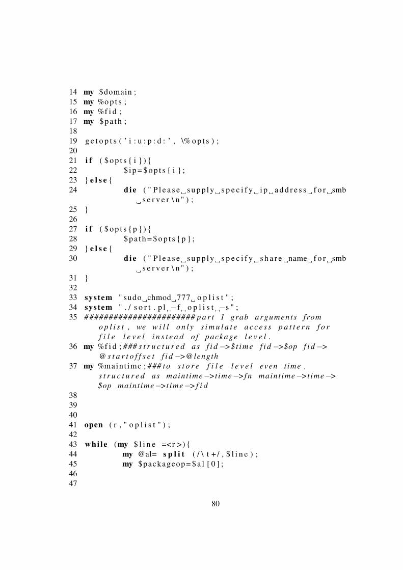
14 my $domain ;15 my %o p t s ;16 my %f i d ;17 my $ p a t h ;1819 g e t o p t s ( ’ i : u : p : d : ’ , \% o p t s ) ;2021 i f ( $ o p t s { i } ) {22 $ i p = $ o p t s { i } ;23 } e l s e {24 d i e ( " P l e a s e s u p p l y s p e c i f y i p a d d r e s s f o r smb
s e r v e r \ n " ) ;25 }2627 i f ( $ o p t s {p } ) {28 $ p a t h = $ o p t s {p } ;29 } e l s e {30 d i e ( " P l e a s e s u p p l y s p e c i f y s h a r e name f o r smb
s e r v e r \ n " ) ;31 }3233 system " sudo chmod 777 o p l i s t " ;34 system " . / s o r t . p l �f o p l i s t �s " ;35 # ###################### p a r t 1 grab arguments from
o p l i s t , we w i l l o n l y s i m u l a t e a c c e s s p a t t e r n f o r
f i l e l e v e l i n s t e a d o f package l e v e l .
36 my %f i d ; ### s t r u c t u r e d as f i d �>$ t i m e f i d �>$op f i d �>
@ s t a r t o f f s e t f i d �>@length
37 my %maint ime ; ### t o s t o r e f i l e l e v e l even t ime ,
s t r u c t u r e d as maint ime�>time�>f n maint ime�>time�>
$op maint ime�>time�>f i d
38394041 open ( r , " o p l i s t " ) ;4243 whi le (my $ l i n e =<r >) {44 my @al= s p l i t ( / \ t + / , $ l i n e ) ;45 my $packageop = $ a l [ 0 ] ;4647
80

48 i f ( $packageop eq "w" | | $packageop eq " r " ) {49 my $ p a c k a g e t i m e = $ a l [ 1 ] ;50 my $ p a c k a g e s t a r t = $ a l [ 2 ] ;51 my $ p a c k a g e l e n g t h = $ a l [ 3 ] ;52 my $ p a c k a g e f i d = $ a l [ 4 ] ;53 my $ p a c k a g e f n = $ a l [ 5 ] ;54 $ p a c k a g e f n =~ s / \ \ \ \ / \ / / g ;5556 i f ( d e f i n e d $ f i d { $ p a c k a g e f i d } ) {57 i f ( $ f i d { $ p a c k a g e f i d }{ t ime }>=
$ p a c k a g e t i m e ) {58 $ f i d { $ p a c k a g e f i d }{ t ime
}= $ p a c k a g e t i m e ; ##
o n l y l o g f i l e f i r s t
a c c e s s t ime , o t h e r
a c c e s s w i l l be
s e q u e n c i a l
59 }6061 } e l s e {62 $ f i d { $ p a c k a g e f i d }{ t ime }=
$ p a c k a g e t i m e ;63 $ f i d { $ p a c k a g e f i d }{ op}=
$packageop ;64 $ f i d { $ p a c k a g e f i d }{ fn }=
$ p a c k a g e f n ;65 }66 push (@{ $ f i d { $ p a c k a g e f i d }{ s t a r t }} ,
$ p a c k a g e s t a r t ) ;67 push (@{ $ f i d { $ p a c k a g e f i d }{ l e n g t h }} ,
$ p a c k a g e l e n g t h ) ;68 }69 }70717273 # i n s e r t f i r s t a c c e s s t i m e t o main t ime
74 foreach my $key ( keys %f i d ) {7576 $main t ime { $ f i d { $key }{ t ime }}{ f i d }= $key ;
81

77 $main t ime { $ f i d { $key }{ t ime }}{ op}= $ f i d { $key }{ op} ;
7879 }8081 #### t e s t area
82 foreach my $ t ime ( s o r t {$a <=>$b } keys %maint ime ) {83 # p r i n t " main t ime t i m e : $ t i m e op : $main t ime { $ t i m e
} { op } f i d : $main t ime { $ t i m e } { f i d } f n : $main t ime { $ t i m e
} { f n } \ n " ;
84 }85 # ###################### p a r t 2 p r e p a r a t i o n p a r t
####################################
86 open ( r2 , " s t r i n g " ) ; ## p r e p a r e f o r w r i t e o p e r a t i o n , i t
w i l l read t h i s random f i l e and w r i t e i t s c o n t e n t t o
t a r g e t f i l e l o c a t i o n
878889 # p r e p a r e t h r e a d poo l f o r l a t e r usage
90 my $poo l = Thread : : Pool�>new (91 {92 worke r s => 1 ,93 do => \&do ,94 }95 ) ;969798 system " u l i m i t �s 16384 " ; # t h i s o p e r a t i o n w i l l
i n c r e a s e t h e s t a c k v a l u e t o 16M f o r t h r e a d i n l i n u x
. By do ing t h i s one c o u l d read more a t once from
smb s e r v e r w i t h o u t " S e g m e n t a t i o n f a u l t ( co re dumped
) "
99100 my $ s t r i n g 1 0 m : s h a r e d = &g e n s t r i n g (10485760) ; # p r e p a r e d
t h e f i x c o n t e n t f o r w r i t e o p e r a t i o n
101102 my @sleep=&s l e e p t i m e ;103104105 # ###################### p a r t 3 s i m u l a t i o n p a r t
####################################
82

106 foreach my $ t ime ( s o r t {$a <=>$b } keys %maint ime ) {107 i f ( $main t ime { $ t ime }{ op } eq " r " ) {108 $pool�>j o b ( \ $ f i d { $main t ime { $ t ime }{ f i d
}}{ fn } , " r " , \@{ $ f i d { $main t ime { $ t ime}{ f i d }}{ s t a r t } } , \@{ $ f i d { $main t ime {$ t ime }{ f i d }}{ l e n g t h } } ) ;
109 }110 i f ( $main t ime { $ t ime }{ op } eq "w" ) {111 $pool�>j o b ( \ $ f i d { $main t ime { $ t ime }{ f i d
}}{ fn } , "w" , \@{ $ f i d { $main t ime { $ t ime}{ f i d }}{ s t a r t } } , \@{ $ f i d { $main t ime {$ t ime }{ f i d }}{ l e n g t h } } ) ;
112 }113114 my $ s l e e p = s h i f t @sleep ;115 $ s l e e p = $ s l e e p ⇤1000000000;116 n a n o s l e e p ( $ s l e e p ) ;117 }118119 $pool�>au toshu tdown ( 1 ) ; # shutdown when o b j e c t i s
d e s t r o y e d
120 $pool�>shutdown ; # w a i t u n t i l a l l j o b s done
121 $pool�>a b o r t ;122123 # ###################### p a r t 4 s u b r u t i n e p a r t
124125 sub do{126 my $smb = new F i l e s y s : : SmbCl ien t ( username => " " ,127 password => " " ,128 workgroup => "
WORKGROUP" ) ;129 my ( $f , $op , $s , $ l ) =@_;130 my $fn = $$f ;131 chomp ( $ fn ) ;132 my $ f i d =0;133 whi le ( 1 ) {134135 $ f i d =$smb�>open ( " smb : / / 1 0 . 0 . 0 . 2 /
s h a r e 2 $ f n " ) o r p r i n t " Can ’ t r e a df i l e : " , $ ! , " $ fn \ n " ;
136 n a n o s l e e p ( 2 0 ) ;
83

137 i f ( $ f i d )138 {139 p r i n t " open s u c c e s s e d \ n " ;140 l a s t ;141 }142 }143 my @ s t a r t =@$s ;144 my @length=@$l ;145 foreach my $key ( keys @ s t a r t ) { ## run each
a c c e s s r e q u e s t f o r one open f i l e w i t h one
t h r e a d
146 $smb�>seek ( $ f i d , $ s t a r t [ $key ] ) ;147 # w h i l e ( $ l e n g t h [ $key ] >104857) {### c u t
t h e r e q u e s t t o max l e n g t h f o r s t a c k s i z e ,
t h i s w i l l i n c r e a s e t h e t h r o u g h p u t
148 # i f ( $op eq " r " ) {
149 # my $a=$smb�>read ( $ f i d
, 1 0 4 8 5 7 ) ;
150 # }
151 # i f ( $op eq "w" ) {
152 # $smb�>w r i t e ( $ f i d ,
$ s t r i n g 1 0 m ) ;
153 # }
154 # $ l e n g t h [ $key ]�=104857;
155 ## }
156157 i f ( $op eq " r " ) {158 my $a=$smb�>read ( $ f i d , $ l e n g t h
[ $key ] ) ;159 }160 i f ( $op eq "w" ) {161 my $ s t r i n g =&g e n s t r i n g ( $ l e n g t h
[ $key ] ) ;162 $smb�>w r i t e ( $ f i d , $ s t r i n g ) ;163 }164165166 }167 $smb�>c l o s e ( $ f i d ) ;168 p r i n t " j o b $fn end \ n " ;169 }
84
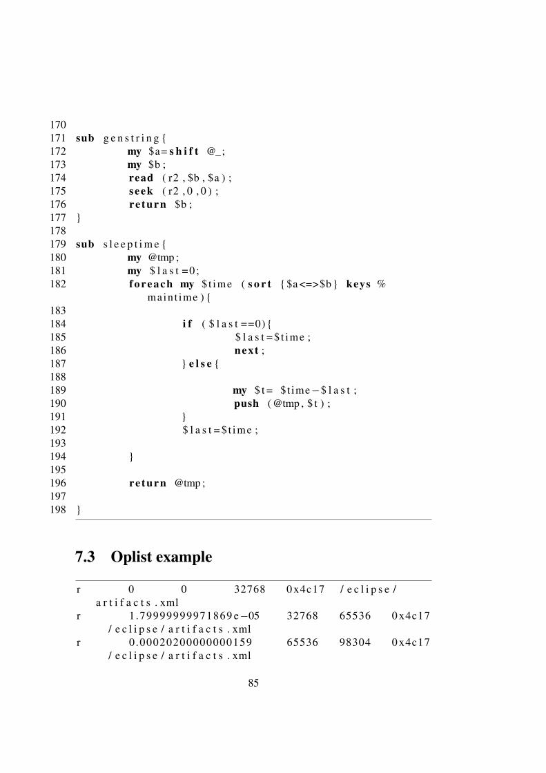
170171 sub g e n s t r i n g {172 my $a= s h i f t @_;173 my $b ;174 read ( r2 , $b , $a ) ;175 seek ( r2 , 0 , 0 ) ;176 re turn $b ;177 }178179 sub s l e e p t i m e {180 my @tmp ;181 my $ l a s t =0 ;182 foreach my $ t ime ( s o r t {$a <=>$b } keys %
maint ime ) {183184 i f ( $ l a s t ==0) {185 $ l a s t = $ t ime ;186 next ;187 } e l s e {188189 my $ t = $t ime�$ l a s t ;190 push (@tmp , $ t ) ;191 }192 $ l a s t = $ t ime ;193194 }195196 re turn @tmp ;197198 }
7.3 Oplist example
r 0 0 32768 0 x4c17 / e c l i p s e /a r t i f a c t s . xml
r 1 .79999999971869 e�05 32768 65536 0 x4c17/ e c l i p s e / a r t i f a c t s . xml
r 0 .00020200000000159 65536 98304 0 x4c17/ e c l i p s e / a r t i f a c t s . xml
85

r 5 .99999999906231 e�06 98304 131072 0 x4c17/ e c l i p s e / a r t i f a c t s . xml
r 1 .00000000102796 e�06 131072 147612 0 x4c17/ e c l i p s e / a r t i f a c t s . xml
r 0 .0558109999999985 0 17920 0 x4c18/ e c l i p s e / e c l i p s e c . exe
r 0 .00697900000000118 0 16536 0 x4c19/ e c l i p s e / ep l�v10 . h tml
r 0 .0918069999999993 0 32768 0 x4c1a/ e c l i p s e / e c l i p s e . exe
r 1 .80000000007396 e�05 32768 65536 0 x4c1a/ e c l i p s e / e c l i p s e . exe
r 2 .99999999953116 e�06 65536 98304 0 x4c1a/ e c l i p s e / e c l i p s e . exe
r 2 .00000000205591 e�06 98304 131072 0 x4c1a/ e c l i p s e / e c l i p s e . exe
r 2 .99999999953116 e�06 131072 163840 0 x4c1a/ e c l i p s e / e c l i p s e . exe
r 1 .9999999985032 e�06 163840 196608 0 x4c1a/ e c l i p s e / e c l i p s e . exe
r 0 .011375000000001 196608 229376 0 x4c1a/ e c l i p s e / e c l i p s e . exe
r 0 .0510629999999992 229376 262144 0 x4c1a/ e c l i p s e / e c l i p s e . exe
r 0 .207333999999999 262144 294912 0 x4c1a/ e c l i p s e / e c l i p s e . exe
r 2 .3999999999802 e�05 294912 312320 0 x4c1a/ e c l i p s e / e c l i p s e . exe
r 0 .00414300000000267 0 514 0 x4c1b/ e c l i p s e / e c l i p s e . i n i
r 0 .0352969999999999 0 32768 0 x4c1c/ e c l i p s e / . e c l i p s e p r o d u c t
r 2 .09999999967181 e�05 32768 65536 0 x4c1c/ e c l i p s e / . e c l i p s e p r o d u c t
r 3 .00000000308387 e�06 65536 98304 0 x4c1c/ e c l i p s e / . e c l i p s e p r o d u c t
r 2 .99999999953116 e�06 98304 131072 0 x4c1c/ e c l i p s e / . e c l i p s e p r o d u c t
r 1 .9999999985032 e�06 131072 163840 0 x4c1c/ e c l i p s e / . e c l i p s e p r o d u c t
86

r 2 .00000000205591 e�06 163840 196608 0 x4c1c/ e c l i p s e / . e c l i p s e p r o d u c t
r 3 .9999999970064 e�06 196608 229376 0 x4c1c/ e c l i p s e / . e c l i p s e p r o d u c t
r 0 .00714900000000185 229376 262144 0 x4c1c/ e c l i p s e / . e c l i p s e p r o d u c t
r 0 .0334219999999981 262144 294912 0 x4c1c/ e c l i p s e / . e c l i p s e p r o d u c t
r 0 .000504000000002947 294912 327680 0 x4c1c/ e c l i p s e / . e c l i p s e p r o d u c t
r 0 .0430089999999979 327680 360448 0 x4c1c/ e c l i p s e / . e c l i p s e p r o d u c t
r 0 .000150000000001427 360448 393216 0 x4c1c/ e c l i p s e / . e c l i p s e p r o d u c t
r 0 .000796999999998604 393216 425984 0 x4c1c/ e c l i p s e / . e c l i p s e p r o d u c t
r 0 .000305000000000888 425984 458752 0 x4c1c/ e c l i p s e / . e c l i p s e p r o d u c t
r 0 .00125699999999895 458752 491520 0 x4c1c/ e c l i p s e / . e c l i p s e p r o d u c t
r 6 .00000000261502 e�06 491520 524288 0 x4c1c/ e c l i p s e / . e c l i p s e p r o d u c t
r 0 .000919999999997145 524288 557056 0 x4c1c/ e c l i p s e / . e c l i p s e p r o d u c t
r 0 .000685000000000713 557056 589824 0 x4c1c/ e c l i p s e / . e c l i p s e p r o d u c t
r 0 .000855999999998858 589824 622592 0 x4c1c/ e c l i p s e / . e c l i p s e p r o d u c t
r 0 .000827000000001021 622592 655360 0 x4c1c/ e c l i p s e / . e c l i p s e p r o d u c t
r 0 .00106699999999904 655360 688128 0 x4c1c/ e c l i p s e / . e c l i p s e p r o d u c t
r 3 .00000000308387 e�06 688128 720896 0 x4c1c/ e c l i p s e / . e c l i p s e p r o d u c t
r 0 .00884799999999686 720896 753664 0 x4c1c/ e c l i p s e / . e c l i p s e p r o d u c t
r 0 .000417000000002332 753664 786432 0 x4c1c/ e c l i p s e / . e c l i p s e p r o d u c t
r 0 .000606999999998692 786432 819200 0 x4c1c/ e c l i p s e / . e c l i p s e p r o d u c t
87
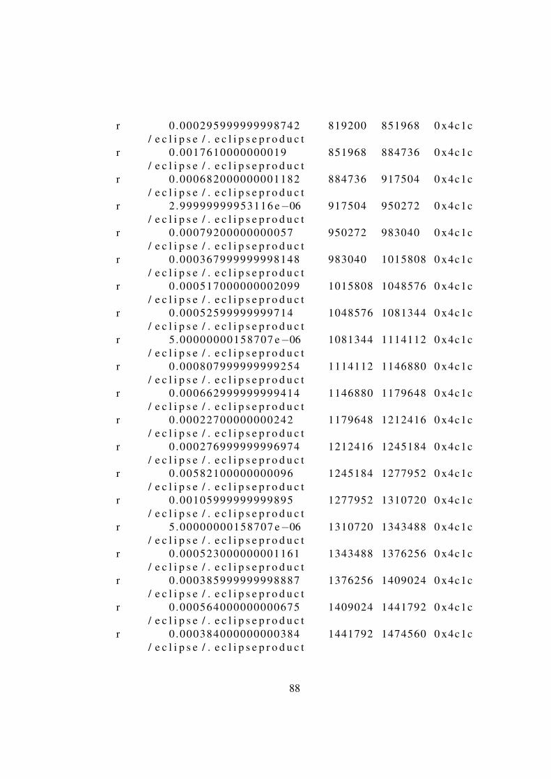
r 0 .000295999999998742 819200 851968 0 x4c1c/ e c l i p s e / . e c l i p s e p r o d u c t
r 0 .0017610000000019 851968 884736 0 x4c1c/ e c l i p s e / . e c l i p s e p r o d u c t
r 0 .000682000000001182 884736 917504 0 x4c1c/ e c l i p s e / . e c l i p s e p r o d u c t
r 2 .99999999953116 e�06 917504 950272 0 x4c1c/ e c l i p s e / . e c l i p s e p r o d u c t
r 0 .00079200000000057 950272 983040 0 x4c1c/ e c l i p s e / . e c l i p s e p r o d u c t
r 0 .000367999999998148 983040 1015808 0 x4c1c/ e c l i p s e / . e c l i p s e p r o d u c t
r 0 .000517000000002099 1015808 1048576 0 x4c1c/ e c l i p s e / . e c l i p s e p r o d u c t
r 0 .00052599999999714 1048576 1081344 0 x4c1c/ e c l i p s e / . e c l i p s e p r o d u c t
r 5 .00000000158707 e�06 1081344 1114112 0 x4c1c/ e c l i p s e / . e c l i p s e p r o d u c t
r 0 .000807999999999254 1114112 1146880 0 x4c1c/ e c l i p s e / . e c l i p s e p r o d u c t
r 0 .000662999999999414 1146880 1179648 0 x4c1c/ e c l i p s e / . e c l i p s e p r o d u c t
r 0 .00022700000000242 1179648 1212416 0 x4c1c/ e c l i p s e / . e c l i p s e p r o d u c t
r 0 .000276999999996974 1212416 1245184 0 x4c1c/ e c l i p s e / . e c l i p s e p r o d u c t
r 0 .00582100000000096 1245184 1277952 0 x4c1c/ e c l i p s e / . e c l i p s e p r o d u c t
r 0 .00105999999999895 1277952 1310720 0 x4c1c/ e c l i p s e / . e c l i p s e p r o d u c t
r 5 .00000000158707 e�06 1310720 1343488 0 x4c1c/ e c l i p s e / . e c l i p s e p r o d u c t
r 0 .000523000000001161 1343488 1376256 0 x4c1c/ e c l i p s e / . e c l i p s e p r o d u c t
r 0 .000385999999998887 1376256 1409024 0 x4c1c/ e c l i p s e / . e c l i p s e p r o d u c t
r 0 .000564000000000675 1409024 1441792 0 x4c1c/ e c l i p s e / . e c l i p s e p r o d u c t
r 0 .000384000000000384 1441792 1474560 0 x4c1c/ e c l i p s e / . e c l i p s e p r o d u c t
88

r 0 .00054399999999788 1474560 1507328 0 x4c1c/ e c l i p s e / . e c l i p s e p r o d u c t
r 0 .000265999999999877 1507328 1540096 0 x4c1c/ e c l i p s e / . e c l i p s e p r o d u c t
r 0 .000934000000000879 1540096 1572864 0 x4c1c/ e c l i p s e / . e c l i p s e p r o d u c t
r 0 .000282999999999589 1572864 1605632 0 x4c1c/ e c l i p s e / . e c l i p s e p r o d u c t
r 0 .000209999999999155 1605632 1638400 0 x4c1c/ e c l i p s e / . e c l i p s e p r o d u c t
r 0 .000615000000003363 1638400 1671168 0 x4c1c/ e c l i p s e / . e c l i p s e p r o d u c t
r 0 .00139999999999674 1671168 1703936 0 x4c1c/ e c l i p s e / . e c l i p s e p r o d u c t
r 0 .000262000000002871 1703936 1736704 0 x4c1c/ e c l i p s e / . e c l i p s e p r o d u c t
r 0 .000237999999999516 1736704 1769472 0 x4c1c/ e c l i p s e / . e c l i p s e p r o d u c t
r 0 .000610999999999251 1769472 1802240 0 x4c1c/ e c l i p s e / . e c l i p s e p r o d u c t
r 0 .000852999999999327 1802240 1835008 0 x4c1c/ e c l i p s e / . e c l i p s e p r o d u c t
r 2 .99999999953116 e�06 1835008 1867776 0 x4c1c/ e c l i p s e / . e c l i p s e p r o d u c t
r 0 .000348000000002457 1867776 1900544 0 x4c1c/ e c l i p s e / . e c l i p s e p r o d u c t
r 0 .000753999999997035 1900544 1933312 0 x4c1c/ e c l i p s e / . e c l i p s e p r o d u c t
r 0 .000505000000000422 1933312 1966080 0 x4c1c/ e c l i p s e / . e c l i p s e p r o d u c t
r 5 .00000000158707 e�06 1966080 1998848 0 x4c1c/ e c l i p s e / . e c l i p s e p r o d u c t
r 0 .00075999999999965 1998848 2031616 0 x4c1c/ e c l i p s e / . e c l i p s e p r o d u c t
r 0 .000236999999998488 2031616 2064384 0 x4c1c/ e c l i p s e / . e c l i p s e p r o d u c t
r 0 .000720000000001164 2064384 2097152 0 x4c1c/ e c l i p s e / . e c l i p s e p r o d u c t
r 0 .000375999999999266 2097152 2129920 0 x4c1c/ e c l i p s e / . e c l i p s e p r o d u c t
89
r 0 .000325000000000131 2129920 2162688 0 x4c1c/ e c l i p s e / . e c l i p s e p r o d u c t
r 0 .000711000000002571 2162688 2195456 0 x4c1c/ e c l i p s e / . e c l i p s e p r o d u c t
r 0 .000552999999996473 2195456 2228224 0 x4c1c/ e c l i p s e / . e c l i p s e p r o d u c t
r 7 .00000000009027 e�06 2228224 2260992 0 x4c1c/ e c l i p s e / . e c l i p s e p r o d u c t
r 0 .000288000000001176 2260992 2293760 0 x4c1c/ e c l i p s e / . e c l i p s e p r o d u c t
r 0 .000852999999999327 2293760 2326528 0 x4c1c/ e c l i p s e / . e c l i p s e p r o d u c t
r 0 .000752000000002084 2326528 2359296 0 x4c1c/ e c l i p s e / . e c l i p s e p r o d u c t
r 0 .000489999999999213 2359296 2392064 0 x4c1c/ e c l i p s e / . e c l i p s e p r o d u c t
r 4 .99999999803435 e�06 2392064 2424832 0 x4c1c/ e c l i p s e / . e c l i p s e p r o d u c t
r 0 .000467000000000439 2424832 2457600 0 x4c1c/ e c l i p s e / . e c l i p s e p r o d u c t
r 5 .00000000158707 e�06 2457600 2490368 0 x4c1c/ e c l i p s e / . e c l i p s e p r o d u c t
r 0 .000541999999999376 2490368 2523136 0 x4c1c/ e c l i p s e / . e c l i p s e p r o d u c t
r 7 .00000000009027 e�06 2523136 2555904 0 x4c1c/ e c l i p s e / . e c l i p s e p r o d u c t
r 0 .00076699999999974 2555904 2588672 0 x4c1c/ e c l i p s e / . e c l i p s e p r o d u c t
r 0 .000410999999999717 2588672 2621440 0 x4c1c/ e c l i p s e / . e c l i p s e p r o d u c t
r 0 .000517000000002099 2621440 2654208 0 x4c1c/ e c l i p s e / . e c l i p s e p r o d u c t
r 0 .000322999999998075 2654208 2686976 0 x4c1c/ e c l i p s e / . e c l i p s e p r o d u c t
r 0 .000707999999999487 2686976 2719744 0 x4c1c/ e c l i p s e / . e c l i p s e p r o d u c t
r 0 .000636000000000081 2719744 2752512 0 x4c1c/ e c l i p s e / . e c l i p s e p r o d u c t
r 6 .00000000261502 e�06 2752512 2785280 0 x4c1c/ e c l i p s e / . e c l i p s e p r o d u c t
90

r 0 .000251999999999697 2785280 2818048 0 x4c1c/ e c l i p s e / . e c l i p s e p r o d u c t
r 0 .00123299999999915 2818048 2850816 0 x4c1c/ e c l i p s e / . e c l i p s e p r o d u c t
r 0 .000555999999999557 2850816 2883584 0 x4c1c/ e c l i p s e / . e c l i p s e p r o d u c t
r 5 .99999999906231 e�06 2883584 2916352 0 x4c1c/ e c l i p s e / . e c l i p s e p r o d u c t
r 0 .000212000000001211 2916352 2949120 0 x4c1c/ e c l i p s e / . e c l i p s e p r o d u c t
r 0 .00179299999999927 2949120 2981888 0 x4c1c/ e c l i p s e / . e c l i p s e p r o d u c t
r 8 .40000000010832 e�05 2981888 3014656 0 x4c1c/ e c l i p s e / . e c l i p s e p r o d u c t
r 0 .000298000000000798 3014656 3047424 0 x4c1c/ e c l i p s e / . e c l i p s e p r o d u c t
r 0 .000163999999998055 3047424 3080192 0 x4c1c/ e c l i p s e / . e c l i p s e p r o d u c t
r 0 .00169800000000109 3080192 3112960 0 x4c1c/ e c l i p s e / . e c l i p s e p r o d u c t
r 0 .000537999999998817 3112960 3145728 0 x4c1c/ e c l i p s e / . e c l i p s e p r o d u c t
r 0 .000409000000001214 3145728 3178496 0 x4c1c/ e c l i p s e / . e c l i p s e p r o d u c t
r 0 .000209999999999155 3178496 3211264 0 x4c1c/ e c l i p s e / . e c l i p s e p r o d u c t
r 0 .00102500000000205 3211264 3244032 0 x4c1c/ e c l i p s e / . e c l i p s e p r o d u c t
r 0 .000150999999998902 3244032 3276800 0 x4c1c/ e c l i p s e / . e c l i p s e p r o d u c t
r 0 .000270000000000437 3276800 3309568 0 x4c1c/ e c l i p s e / . e c l i p s e p r o d u c t
r 0 .000239000000000544 3309568 3342336 0 x4c1c/ e c l i p s e / . e c l i p s e p r o d u c t
r 0 .00137999999999749 3342336 3375104 0 x4c1c/ e c l i p s e / . e c l i p s e p r o d u c t
r 0 .000717999999999108 3375104 3407872 0 x4c1c/ e c l i p s e / . e c l i p s e p r o d u c t
r 0 .000442000000003162 3407872 3440640 0 x4c1c/ e c l i p s e / . e c l i p s e p r o d u c t
91

r 0 .000276999999996974 3440640 3473408 0 x4c1c/ e c l i p s e / . e c l i p s e p r o d u c t
r 0 .000220000000002329 3473408 3506176 0 x4c1c/ e c l i p s e / . e c l i p s e p r o d u c t
r 0 .000467999999997915 3506176 3538944 0 x4c1c/ e c l i p s e / . e c l i p s e p r o d u c t
r 0 .000239000000000544 3538944 3571712 0 x4c1c/ e c l i p s e / . e c l i p s e p r o d u c t
r 0 .00105100000000036 3571712 3604480 0 x4c1c/ e c l i p s e / . e c l i p s e p r o d u c t
r 0 .000830000000000553 3604480 3637248 0 x4c1c/ e c l i p s e / . e c l i p s e p r o d u c t
r 2 .99999999953116 e�06 3637248 3670016 0 x4c1c/ e c l i p s e / . e c l i p s e p r o d u c t
r 0 .000358000000002079 3670016 3702784 0 x4c1c/ e c l i p s e / . e c l i p s e p r o d u c t
r 0 .000167999999998614 3702784 3735552 0 x4c1c/ e c l i p s e / . e c l i p s e p r o d u c t
r 0 .00201900000000066 3735552 3768320 0 x4c1c/ e c l i p s e / . e c l i p s e p r o d u c t
r 0 .000394999999997481 3768320 3801088 0 x4c1c/ e c l i p s e / . e c l i p s e p r o d u c t
r 0 .000499000000001359 3801088 3833856 0 x4c1c/ e c l i p s e / . e c l i p s e p r o d u c t
r 5 .99999999906231 e�06 3833856 3866624 0 x4c1c/ e c l i p s e / . e c l i p s e p r o d u c t
r 0 .00130700000000061 3866624 3899392 0 x4c1c/ e c l i p s e / . e c l i p s e p r o d u c t
r 0 .000299000000001826 3899392 3932160 0 x4c1c/ e c l i p s e / . e c l i p s e p r o d u c t
r 0 .000153999999998433 3932160 3964928 0 x4c1c/ e c l i p s e / . e c l i p s e p r o d u c t
r 0 .000272999999999968 3964928 3997696 0 x4c1c/ e c l i p s e / . e c l i p s e p r o d u c t
r 0 .00153099999999995 3997696 4030464 0 x4c1c/ e c l i p s e / . e c l i p s e p r o d u c t
r 0 .000398000000000565 4030464 4063232 0 x4c1c/ e c l i p s e / . e c l i p s e p r o d u c t
r 4 .00000000055911 e�06 4063232 4096000 0 x4c1c/ e c l i p s e / . e c l i p s e p r o d u c t
92

r 1 .9999999985032 e�06 4096000 4128768 0 x4c1c/ e c l i p s e / . e c l i p s e p r o d u c t
r 0 .000900000000001455 4128768 4161536 0 x4c1c/ e c l i p s e / . e c l i p s e p r o d u c t
r 0 .000464000000000908 4161536 4194304 0 x4c1c/ e c l i p s e / . e c l i p s e p r o d u c t
r 0 .000417999999999807 4194304 4227072 0 x4c1c/ e c l i p s e / . e c l i p s e p r o d u c t
r 4 .99999999803435 e�06 4227072 4259840 0 x4c1c/ e c l i p s e / . e c l i p s e p r o d u c t
r 0 .00309599999999932 4259840 4292608 0 x4c1c/ e c l i p s e / . e c l i p s e p r o d u c t
r 0 .00023400000000251 4292608 4325376 0 x4c1c/ e c l i p s e / . e c l i p s e p r o d u c t
r 0 .000440999999998581 4325376 4358144 0 x4c1c/ e c l i p s e / . e c l i p s e p r o d u c t
r 0 .00045599999999979 4358144 4390912 0 x4c1c/ e c l i p s e / . e c l i p s e p r o d u c t
r 0 .000461000000001377 4390912 4423680 0 x4c1c/ e c l i p s e / . e c l i p s e p r o d u c t
r 0 .000478999999998564 4423680 4456448 0 x4c1c/ e c l i p s e / . e c l i p s e p r o d u c t
r 0 .000427000000001954 4456448 4489216 0 x4c1c/ e c l i p s e / . e c l i p s e p r o d u c t
r 2 .99999999953116 e�06 4489216 4521984 0 x4c1c/ e c l i p s e / . e c l i p s e p r o d u c t
r 0 .00115399999999966 4521984 4554752 0 x4c1c/ e c l i p s e / . e c l i p s e p r o d u c t
r 2 .99999999953116 e�06 4554752 4587520 0 x4c1c/ e c l i p s e / . e c l i p s e p r o d u c t
r 0 .000408000000000186 4587520 4620288 0 x4c1c/ e c l i p s e / . e c l i p s e p r o d u c t
r 5 .99999999906231 e�06 4620288 4653056 0 x4c1c/ e c l i p s e / . e c l i p s e p r o d u c t
r 0 .00112199999999874 4653056 4685824 0 x4c1c/ e c l i p s e / . e c l i p s e p r o d u c t
r 0 .000679000000001651 4685824 4718592 0 x4c1c/ e c l i p s e / . e c l i p s e p r o d u c t
r 0 .000223999999999336 4718592 4751360 0 x4c1c/ e c l i p s e / . e c l i p s e p r o d u c t
93

r 0 .000154000000001986 4751360 4784128 0 x4c1c/ e c l i p s e / . e c l i p s e p r o d u c t
r 0 .0027659999999976 4784128 4816896 0 x4c1c/ e c l i p s e / . e c l i p s e p r o d u c t
r 0 .000410000000002242 4816896 4849664 0 x4c1c/ e c l i p s e / . e c l i p s e p r o d u c t
r 4 .99999999803435 e�06 4849664 4882432 0 x4c1c/ e c l i p s e / . e c l i p s e p r o d u c t
r 0 .000206999999999624 4882432 4915200 0 x4c1c/ e c l i p s e / . e c l i p s e p r o d u c t
r 0 .0016820000000024 4915200 4947968 0 x4c1c/ e c l i p s e / . e c l i p s e p r o d u c t
r 2 .99999999953116 e�06 4947968 4980736 0 x4c1c/ e c l i p s e / . e c l i p s e p r o d u c t
r 1 .00000000102796 e�06 4980736 5013504 0 x4c1c/ e c l i p s e / . e c l i p s e p r o d u c t
r 0 .000242000000000075 5013504 5046272 0 x4c1c/ e c l i p s e / . e c l i p s e p r o d u c t
r 0 .00131499999999818 5046272 5079040 0 x4c1c/ e c l i p s e / . e c l i p s e p r o d u c t
r 0 .000212000000001211 5079040 5111808 0 x4c1c/ e c l i p s e / . e c l i p s e p r o d u c t
r 0 .000480999999997067 5111808 5144576 0 x4c1c/ e c l i p s e / . e c l i p s e p r o d u c t
r 4 .00000000055911 e�06 5144576 5177344 0 x4c1c/ e c l i p s e / . e c l i p s e p r o d u c t
r 0 .000728000000002282 5177344 5210112 0 x4c1c/ e c l i p s e / . e c l i p s e p r o d u c t
r 0 .000363000000000113 5210112 5242880 0 x4c1c/ e c l i p s e / . e c l i p s e p r o d u c t
r 0 .000500999999999863 5242880 5275648 0 x4c1c/ e c l i p s e / . e c l i p s e p r o d u c t
r 5 .90000000002533 e�05 5275648 5308416 0 x4c1c/ e c l i p s e / . e c l i p s e p r o d u c t
r 0 .0030179999999973 5308416 5341184 0 x4c1c/ e c l i p s e / . e c l i p s e p r o d u c t
r 0 .0004489999999997 5341184 5373952 0 x4c1c/ e c l i p s e / . e c l i p s e p r o d u c t
r 6 .00000000261502 e�06 5373952 5406720 0 x4c1c/ e c l i p s e / . e c l i p s e p r o d u c t
94

r 0 .000379999999999825 5406720 5439488 0 x4c1c/ e c l i p s e / . e c l i p s e p r o d u c t
r 0 .000824999999998965 5439488 5472256 0 x4c1c/ e c l i p s e / . e c l i p s e p r o d u c t
r 0 .000617999999999341 5472256 5505024 0 x4c1c/ e c l i p s e / . e c l i p s e p r o d u c t
r 0 .000372000000002259 5505024 5537792 0 x4c1c/ e c l i p s e / . e c l i p s e p r o d u c t
r 0 .000593999999999539 5537792 5570560 0 x4c1c/ e c l i p s e / . e c l i p s e p r o d u c t
r 0 .000498000000000332 5570560 5603328 0 x4c1c/ e c l i p s e / . e c l i p s e p r o d u c t
r 0 .000258999999999787 5603328 5636096 0 x4c1c/ e c l i p s e / . e c l i p s e p r o d u c t
r 0 .000308000000000419 5636096 5668864 0 x4c1c/ e c l i p s e / . e c l i p s e p r o d u c t
r 0 .000418999999997283 5668864 5701632 0 x4c1c/ e c l i p s e / . e c l i p s e p r o d u c t
r 0 .000845000000001761 5701632 5734400 0 x4c1c/ e c l i p s e / . e c l i p s e p r o d u c t
r 0 .000378999999998797 5734400 5767168 0 x4c1c/ e c l i p s e / . e c l i p s e p r o d u c t
r 0 .000226000000001392 5767168 5799936 0 x4c1c/ e c l i p s e / . e c l i p s e p r o d u c t
r 0 .000272999999999968 5799936 5832704 0 x4c1c/ e c l i p s e / . e c l i p s e p r o d u c t
r 0 .000554999999998529 5832704 5865472 0 x4c1c/ e c l i p s e / . e c l i p s e p r o d u c t
r 0 .000680000000002678 5865472 5898240 0 x4c1c/ e c l i p s e / . e c l i p s e p r o d u c t
r 0 .000490999999996689 5898240 5931008 0 x4c1c/ e c l i p s e / . e c l i p s e p r o d u c t
95

Bibliography
[1] AVISHAY TRAEGER, EREZ ZADOKA, NIKOLAI JOUKOV, CHARLESP. WRIGHT, “Nine Year Study of File System and Storage Benchmarking”.ACM. 2008.
[2] Christina Delimitrou, Sriram Sankar, Kushagra Vaid, Christos Kozyrakis,“Accurate Modeling and Generation of Storage I/O for Datacenter Work-loads”. Exascale Evaluation and Research Techniques (EXERT) Work-shop.2011.
[3] Ningning Zhu, Jiawu Chen, Tzi-Cker Chiueh, “TBBT: Scalable and Accu-rate Trace Replay for File Server Evaluation”. FAST. 2005.
[4] Jon Tate, Pall Beck, Hector Hugo Ibarra, Shanmuganathan Kumaravel, LiborMiklas, “Introduction to Storage Area Networks and System Networking”.
[5] Ralph O. Weber, ”SCSI Architecture Model - 3 (SAM-3)”. T10 TechnicalCommittee. 16 March 2002.
[6] Jelmer R. Vernooij, “The Official Samba-4 HOWTO”.http://www.samba.org/samba/docs/man/Samba4-HOWTO/protocol.html
[7] Jose Barreto, “SMB remote file protocol(including SMB 3.0)”. @StorageNetworking Industry Association.
[8] Mircrosoft, “Common Internet File System (CIFS) Protocol”.
[9] IDC, http://online.wsj.com/article/BT-CO-20131106-709604.html.
[10] J. C. Mogul, ”Brittle metrics in operating systems research”. Proceedings of7th Workshop on Hot Topics in Operating Systems. January 1999.
[11] IBM, “Network file systems and Linux”.http://www.ibm.com/developerworks/library/l-network-filesystems/.
96

[12] Kavalanekar S, Worthington B, Qi Zhang, Sharda V, “Characterizationof storage workload traces from production Windows Servers”. WorkloadCharacterization, 2008. IISWC 2008.
[13] J. Katcher. “PostMark: A New Filesystem Benchmark”.Technical Report TR3022, Network Appliance, 1997.www.netapp.com/tech_library/3022.html.
[14] VERITAS Software. VERITAS File Server Edition Performance Brief: APostMark 1.11 Benchmark Comparison. Technical report, Veritas SoftwareCorporation, June 1999. http://eval.veritas.com/webfiles/docs/fsedition-postmark.pdf.
[15] Transaction Processing Performance Council. Transaction Processing Per-formance Council. www.tpc.org, 2005.
[16] SPEC. The SPEC Organization. www.spec.org/, April 2005.
[17] SPC. Storage Performance Council, 2007. www.storageperformance.org.
[18] R. Coker. The Bonnie++ home page. www.coker.com.au/bonnie++, 2001.
[19] W. Akkerman. strace software home page. www.liacs.nl/~wichert/strace/,2002.
[20] L. Mummert and M. Satyanarayanan. Long term distributed file referencetracing: Implementation and experience. Technical Report CMU-CS-94-213, Carnegie Mellon University, Pittsburgh, PA, 1994.
[21] J. Ousterhout, H. Costa, D. Harrison, J. Kunze, M. Kupfer, and J. Thompson.A Trace-Driven Analysis of the UNIX 4.2 BSD File System. In Proceedingsof the 10th ACM Symposium on Operating System Principles, pp. 15-24,Orcas Island, WA, December 1985
[22] D. Ellard and M. Seltzer. New NFS Tracing Tools and Techniques for Sys-tem Analysis. In Proceedings of the Annual USENIX Conference on LargeInstallation Systems Administration, San Diego, CA, October 2003.
[23] M. Blaze. NFS Tracing by Passive Network Monitoring. In Proceedings ofthe USENIX Winter Conference, San Francisco, CA, January 1992.
[24] C. Ruemmler and J. Wilkes. UNIX Disk Access Patterns. In Proceedings ofthe Winter USENIX Technical Conference, pp. 405-420, San Diego, CA,January 1993.
97

[25] J. Flinn, S. Sinnamohideen, N. Tolia, and M. Satyanaryanan. Data Stagingon Untrusted Surrogates. In Proceedings of the 2nd USENIX Conference onFile and Storage Technologies, pp. 15-28, San Francisco, CA, March 2003.
[26] N. Tolia, J. Harkes, M. Kozuch, and M. Satyanarayanan. IntegratingPortable and Distributed Storage. In Proceedings of the 3rd USENIX Con-ference on File and Storage Technologies, pp. 227-238, San Francisco, CA,March/April 2004.
[27] Z. N. J. Peterson, R. Burns, G. Ateniese, and S. Bono. Design and implemen-tation of verifiable audit trails for a versioning file system. In Proceedings ofthe 5th USENIX Conference on File and Storage Technologies, pp. 93-106,San Jose, CA, February 2007.
[28] V. Prabhakaran, A. C. Arpaci-Dusseau, and R. H. Arpaci-Dussea. Analy-sis and Evolution of Journaling File Systems. In Proceedings of the AnnualUSENIX Technical Conference, pp. 105-120, Anaheim, CA, April 2005.
[29] E. Anderson, M. Kallahalla, M. Uysal, and R. Swaminathan. Buttress: AToolkit for Flexible and High Fidelity I/O Benchmarking. In Proceedings ofthe 3rd USENIX Conference on File and Storage Technologies, pp. 45-58,San Francisco, CA, March/April 2004.
[30] CodeFX. “CIFS Explained”. 2001.
98