A beginner’s course in finite volume approximation

of scalar conservation laws

Pamplona – Pau – Toulouse – Zaragoza summer school on

nonlinear conservation laws

Jaca 11-13/09/2008

Jerome Droniou1

Version: October 10th, 2008

This is a first version, with probably typos errors (but hopefully no mathematical mistake...); feelfree to contact me (see footnote) if you happen to notice some.

1Departement de Mathematiques, UMR CNRS 5149, CC 051, Universite Montpellier II, Place Eugene Bataillon, 34095Montpellier cedex 5, France. email: droniou@math.univ-montp2.fr

Contents

1 Schemes for linear transport equations 31.1 Introduction, principle of the finite volume scheme . . . . . . . . . . . . . . . . . . . . . . 31.2 Centered scheme . . . . . . . . . . . . . . . . . . . . . . . . . . . . . . . . . . . . . . . . . 41.3 Upwind scheme . . . . . . . . . . . . . . . . . . . . . . . . . . . . . . . . . . . . . . . . . . 5

1.3.1 L∞ stability and convergence . . . . . . . . . . . . . . . . . . . . . . . . . . . . . . 61.3.2 Relation with the discretization of convection-diffusion equations . . . . . . . . . . 91.3.3 About the time-implicit discretization . . . . . . . . . . . . . . . . . . . . . . . . . 11

2 Schemes for non-linear conservation laws 132.1 Introduction . . . . . . . . . . . . . . . . . . . . . . . . . . . . . . . . . . . . . . . . . . . . 132.2 Monotone schemes . . . . . . . . . . . . . . . . . . . . . . . . . . . . . . . . . . . . . . . . 13

2.2.1 A first idea . . . . . . . . . . . . . . . . . . . . . . . . . . . . . . . . . . . . . . . . 142.2.2 General monotone schemes, L∞ stability . . . . . . . . . . . . . . . . . . . . . . . . 152.2.3 Examples of monotone fluxes, interpretation of the CFL condition . . . . . . . . . 172.2.4 Numerical diffusion . . . . . . . . . . . . . . . . . . . . . . . . . . . . . . . . . . . . 19

2.3 Study of monotone schemes . . . . . . . . . . . . . . . . . . . . . . . . . . . . . . . . . . . 192.3.1 BV estimates . . . . . . . . . . . . . . . . . . . . . . . . . . . . . . . . . . . . . . . 192.3.2 Discrete entropy inequalities . . . . . . . . . . . . . . . . . . . . . . . . . . . . . . 212.3.3 Convergence of the scheme . . . . . . . . . . . . . . . . . . . . . . . . . . . . . . . 22

2.4 Some numerical results . . . . . . . . . . . . . . . . . . . . . . . . . . . . . . . . . . . . . . 242.5 Semi-linear parabolic equations . . . . . . . . . . . . . . . . . . . . . . . . . . . . . . . . . 242.6 Two concluding remarks . . . . . . . . . . . . . . . . . . . . . . . . . . . . . . . . . . . . . 28

2.6.1 Implicit discretization of the fluxes . . . . . . . . . . . . . . . . . . . . . . . . . . . 282.6.2 Convergence without BV estimates . . . . . . . . . . . . . . . . . . . . . . . . . . . 28

3 MUSCL methods 303.1 Position of the problem, principle of MUSCL schemes . . . . . . . . . . . . . . . . . . . . 303.2 General stability and entropy lemmas . . . . . . . . . . . . . . . . . . . . . . . . . . . . . 303.3 Example of a MUSCL scheme . . . . . . . . . . . . . . . . . . . . . . . . . . . . . . . . . . 323.4 Numerical results . . . . . . . . . . . . . . . . . . . . . . . . . . . . . . . . . . . . . . . . . 34

1

SummaryIn this lecture, we present and study some methods to discretize scalar conservation laws ∂tu+∂xf(u) = 0.Considering first the case of a linear equation (f(u) = cu) we try and understand a basic construction ofnumerical schemes (using finite volume techniques) and the issues related, mainly concerning the stabilityof the method. We then introduce the principle of monotone schemes for general non-linear equations,and give some classical examples (Lax-Friedrichs, Godunov); we try to explain the concept of numericaldiffusion associated with such schemes (and its link with the discretization of parabolic equations), andwe give some elements of study: stability, discrete entropy inequalities, convergence in the BV case.The numerical diffusion introduced by monotone fluxes allow to stabilize the scheme, but gives poorapproximations of the qualitative properties of the continuous solution (shocks, rarefaction waves...); inthe last chapter, we introduce some higher order methods (MUSCL techniques) which allow to obtainbetter approximations.

2

Chapter 1

Schemes for linear transportequations

1.1 Introduction, principle of the finite volume scheme

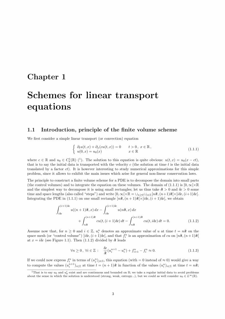
We first consider a simple linear transport (or convection) equation{∂tu(t, x) + ∂x(cu(t, x)) = 0 t > 0 , x ∈ R ,u(0, x) = u0(x) x ∈ R (1.1.1)

where c ∈ R and u0 ∈ C1b (R) (1). The solution to this equation is quite obvious: u(t, x) = u0(x − ct),

that is to say the initial data is transported with the velocity c (the solution at time t is the initial datatranslated by a factor ct). It is however interesting to study numerical approximations for this simpleproblem, since it allows to exhibit the main issues which arise for general non-linear conservation laws.

The principle to construct a finite volume scheme for a PDE is to decompose the domain into small parts(the control volumes) and to integrate the equation on these volumes. The domain of (1.1.1) is [0,∞[×Rand the simplest way to decompose it is using small rectangles; let us thus take δt > 0 and δx > 0 sometime and space lengths (also called “steps”) and write [0,∞[×R = ∪n≥0∪i∈Z [nδt, (n+1)δt[×[iδx, (i+1)δx[.Integrating the PDE in (1.1.1) on one small rectangle [nδt, (n+ 1)δt[×[iδx, (i+ 1)δx[, we obtain∫ (i+1)δx

iδx

u((n+ 1)δt, x) dx−∫ (i+1)δx

iδx

u(nδt, x) dx

+

∫ (n+1)δt

nδt

cu(t, (i+ 1)δx) dt−∫ (n+1)δt

nδt

cu(t, iδx) dt = 0. (1.1.2)

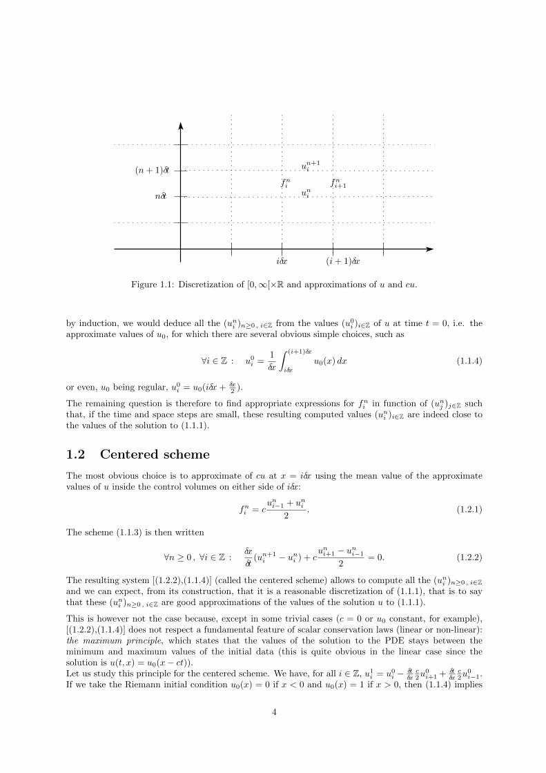
Assume now that, for n ≥ 0 and i ∈ Z, uni denotes an approximate value of u at time t = nδt on thespace mesh (or “control volume”) [iδx, (i+ 1)δx[, and that fni is an approximation of cu on [nδt, (n+ 1)δt[at x = iδx (see Figure 1.1). Then (1.1.2) divided by δt leads

∀n ≥ 0 , ∀i ∈ Z :δx

δt(un+1i − uni ) + fni+1 − fni ≈ 0. (1.1.3)

If we could now express fni in terms of (unj )j∈Z, this equation (with = 0 instead of ≈ 0) would give a way

to compute the values (un+1i )i∈Z at time t = (n + 1)δt in function of the values (uni )i∈Z at time t = nδt;

1That is to say u0 and u′0 exist and are continuous and bounded on R; we take a regular initial data to avoid problemsabout the sense in which the solution is understood (strong, weak, entropy...), but we could as well consider u0 ∈ L∞(R).

3

(i+ 1)δxiδx

nδt

(n+ 1)δt

fni+1fni

un+1i

uni

Figure 1.1: Discretization of [0,∞[×R and approximations of u and cu.

by induction, we would deduce all the (uni )n≥0 , i∈Z from the values (u0i )i∈Z of u at time t = 0, i.e. theapproximate values of u0, for which there are several obvious simple choices, such as

∀i ∈ Z : u0i =1

δx

∫ (i+1)δx

iδx

u0(x) dx (1.1.4)

or even, u0 being regular, u0i = u0(iδx+ δx2 ).

The remaining question is therefore to find appropriate expressions for fni in function of (unj )j∈Z suchthat, if the time and space steps are small, these resulting computed values (uni )i∈Z are indeed close tothe values of the solution to (1.1.1).

1.2 Centered scheme

The most obvious choice is to approximate of cu at x = iδx using the mean value of the approximatevalues of u inside the control volumes on either side of iδx:

fni = cuni−1 + uni

2. (1.2.1)

The scheme (1.1.3) is then written

∀n ≥ 0 , ∀i ∈ Z :δx

δt(un+1i − uni ) + c

uni+1 − uni−12

= 0. (1.2.2)

The resulting system [(1.2.2),(1.1.4)] (called the centered scheme) allows to compute all the (uni )n≥0 , i∈Zand we can expect, from its construction, that it is a reasonable discretization of (1.1.1), that is to saythat these (uni )n≥0 , i∈Z are good approximations of the values of the solution u to (1.1.1).

This is however not the case because, except in some trivial cases (c = 0 or u0 constant, for example),[(1.2.2),(1.1.4)] does not respect a fundamental feature of scalar conservation laws (linear or non-linear):the maximum principle, which states that the values of the solution to the PDE stays between theminimum and maximum values of the initial data (this is quite obvious in the linear case since thesolution is u(t, x) = u0(x− ct)).Let us study this principle for the centered scheme. We have, for all i ∈ Z, u1i = u0i − δt

δxc2u

0i+1 + δt

δxc2u

0i−1.

If we take the Riemann initial condition u0(x) = 0 if x < 0 and u0(x) = 1 if x > 0, then (1.1.4) implies

4

u0j = 0 for all j < 0 and u0j = 1 for all j ≥ 0. Thus,

u1−1 = − δtδx

c

2and u10 = 1− δt

δx

c

2.

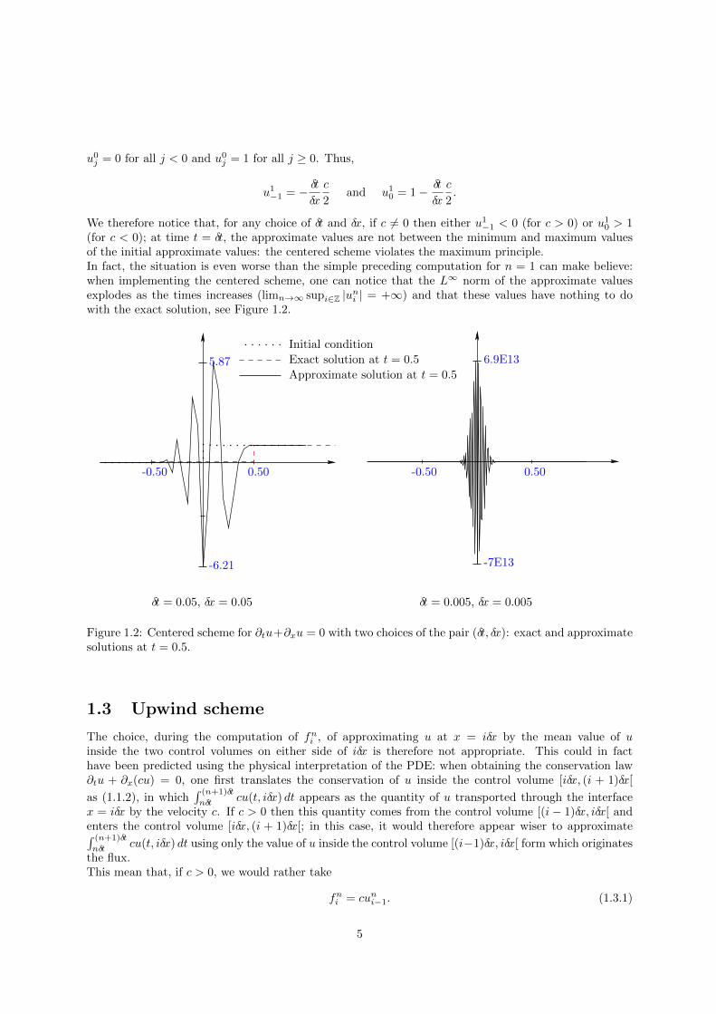
We therefore notice that, for any choice of δt and δx, if c 6= 0 then either u1−1 < 0 (for c > 0) or u10 > 1(for c < 0); at time t = δt, the approximate values are not between the minimum and maximum valuesof the initial approximate values: the centered scheme violates the maximum principle.In fact, the situation is even worse than the simple preceding computation for n = 1 can make believe:when implementing the centered scheme, one can notice that the L∞ norm of the approximate valuesexplodes as the times increases (limn→∞ supi∈Z |uni | = +∞) and that these values have nothing to dowith the exact solution, see Figure 1.2.

-6.21

5.87

δt = 0.05, δx = 0.05 δt = 0.005, δx = 0.005

-7E13

6.9E13

-0.50 0.50 -0.50 0.50

Initial condition

Exact solution at t = 0.5

Approximate solution at t = 0.5

Figure 1.2: Centered scheme for ∂tu+∂xu = 0 with two choices of the pair (δt, δx): exact and approximatesolutions at t = 0.5.

1.3 Upwind scheme

The choice, during the computation of fni , of approximating u at x = iδx by the mean value of uinside the two control volumes on either side of iδx is therefore not appropriate. This could in facthave been predicted using the physical interpretation of the PDE: when obtaining the conservation law∂tu + ∂x(cu) = 0, one first translates the conservation of u inside the control volume [iδx, (i + 1)δx[

as (1.1.2), in which∫ (n+1)δt

nδtcu(t, iδx) dt appears as the quantity of u transported through the interface

x = iδx by the velocity c. If c > 0 then this quantity comes from the control volume [(i − 1)δx, iδx[ andenters the control volume [iδx, (i + 1)δx[; in this case, it would therefore appear wiser to approximate∫ (n+1)δt

nδtcu(t, iδx) dt using only the value of u inside the control volume [(i−1)δx, iδx[ form which originates

the flux.This mean that, if c > 0, we would rather take

fni = cuni−1. (1.3.1)

5

Of course, if c < 0, the same reasoning would lead to choosing fni = cuni . From now on, let us consideronly the case c > 0; with the choice (1.3.1), (1.1.3) is written

∀n ≥ 0 , ∀i ∈ Z :δx

δt(un+1i − uni ) + cuni − cuni−1 = 0. (1.3.2)

The scheme [(1.3.2),(1.1.4)] is called the upwind scheme, precisely because it is constructed using theupwind (with respect to the velocity c) choice (1.3.1) to compute the flux values.

1.3.1 L∞ stability and convergence

On the contrary to the centered scheme, the upwind scheme respects the maximum principle and istherefore L∞ stable: we can prove a L∞ bound on the approximate values.

Proposition 1.3.1 (Stability of the upwind scheme for the linear transport equation) Let c > 0 andassume that δt > 0 and δx > 0 are such that

δt

δx≤ 1

c. (1.3.3)

If (uni )n≥0 , i∈Z satisfies [(1.3.2),(1.1.4)], then

∀n ≥ 0 ,∀i ∈ Z : infj∈Z

unj ≤ un+1i ≤ sup

j∈Zunj . (1.3.4)

In particular, all the values (uni )n≥0 , i∈Z are between the infimum and supremum values of u0 and

supn≥0 , i∈Z

|uni | ≤ ||u0||L∞(R).

Remark 1.3.2 The condition (1.3.3), linking the discretization steps with the velocity and called theCFL condition (for “Courant-Friedrichs-Levy”), states that a small space step imposes a small time step:if the space step is divided by 10, then the time step must also be divided by 10. We will further discussthis condition in Sections 1.3.2 and 2.2.3.

Proof of Proposition 1.3.1The proof is completely trivial if we rewrite (1.3.2) in the following way:

un+1i = uni −

δt

δxcuni +

δt

δxcuni−1 =

(1− δt

δxc

)uni +

δt

δxcuni−1.

The sum of 1 − δtδxc and δt

δxc is equal to 1 and, under the condition (1.3.3), both these terms are non-

negative; hence, un+1i appears as a convex combination of uni and uni−1, and is therefore between the

minimum and maximum value of these two real numbers. Relation (1.3.4) then follows, and the rest ofthe properties stated in the proposition are easy consequences of this relation.

We can now easily prove that the upwind scheme for (1.1.1) converges, i.e. that, for δt and δx small, thevalues (uni )n≥0 , i∈Z computed by [(1.3.2),(1.1.4)] are indeed close (at least in a weak sense) to the valuesof the solution to (1.1.1)

Theorem 1.3.3 (Convergence of the upwind scheme for linear transport equations) Let c > 0. Forδt > 0 and δx > 0, let uδt,δx : [0,∞[×R→ R be the function equal to uni on [nδt, (n+ 1)δt[×[iδx, (i+ 1)δx[for all n ≥ 0 and i ∈ Z. Then, as δt and δx tend to 0 while satisfying the CFL condition (1.3.3), uδt,δxconverges in L∞(]0,∞[×R) weak-∗ to the solution u of (1.1.1).

6

Remark 1.3.4 In fact, the convergence is much stronger than a weak-∗ convergence, as we will seein Chapter 2. However, since (1.1.1) is linear, the weak convergence is enough to pass to the limit inthe numerical scheme and we therefore only state this weak convergence in order to avoid unnecessarycomplexity at this stage.

Proof of Theorem 1.3.3Proposition 1.3.1 implies that, as δt and δx tend to 0 while satisfying (1.3.3), uδt,δx remains bounded inL∞(]0,∞[×R). Up to a subsequence, we can therefore assume that it converges in L∞ weak-∗ to some u;if we prove that any such limit u of a subsequence of uδt,δx is the weak solution to (1.1.1) then, this weaksolution being unique (the equation is linear), this will show that the whole sequence uδt,δx converges tothis solution and will complete the proof.Let us therefore consider that uδt,δx → u weak-∗ and prove that u is a weak solution to (1.1.1), i.e. thatfor all ϕ ∈ C∞c ([0,∞[×R),∫ ∞

0

∫Ru(t, x) (∂tϕ(t, x) + c∂xϕ(t, x)) dtdx+

∫Ru0(x)ϕ(0, x) dx = 0. (1.3.5)

Take ϕ such a regular function and define ϕni = 1δt

1δx

∫ (n+1)δt

nδt

∫ (i+)1)δx

iδxϕ(t, x) dtdx. Multiplying (1.3.2) by

δtϕni and summing on n ≥ 0 and i ∈ Z (notice that, since ϕ has a compact support, these sums in factonly involve a finite number of indices), we find

0 =∑i∈Z

δx∑n≥0

(un+1i − uni )ϕni + c

∑n≥0

δt∑i∈Z

(uni − uni−1)ϕni . (1.3.6)

But ∑n≥0

(un+1i − uni )ϕni =

∑n≥0

un+1i ϕni −

∑n≥0

uni ϕni

=∑n≥1

uni ϕn−1i −

∑n≥0

uni ϕni

=∑n≥1

uni (ϕn−1i − ϕni )− u0iϕ0i

(this series of manipulation comes down to a discrete integration by parts: the “derivative” un+1i − uni

has been put on ϕ). Using a similar manipulation for the second sum on i ∈ Z in (1.3.6), we obtain

0 =∑i∈Z

δx∑n≥1

δtuniϕn−1i − ϕni

δt−∑i∈Z

δxu0iϕ0i + c

∑n≥0

δt∑i∈Z

δxuniϕni − ϕni+1

δx,

that is to say, owing to the definition of uδt,δx and of u0i ,

0 = −∫ ∞nδt

∫Ruδt,δx(t, x)Γδt,δx(t, x) dtdx−

∫Ru0(x)Θδx(x) dx− c

∫ ∞0

∫Ruδt,δx(t, x)Ξδt,δx(t, x) dtdx (1.3.7)

where Γδt,δx, Θδx and Ξδt,δx are defined by

Γδt,δx =ϕni − ϕ

n−1i

δton [nδt, (n+ 1)δt[×[iδx, (i+ 1)δx[,

Θδx = ϕ0i on [iδx, (i+ 1)δx[,

Ξδt,δx =ϕni+1 − ϕni

δxon [nδt, (n+ 1)δt[×[iδx, (i+ 1)δx[.

By regularity of ϕ, we have Γδt,δx → ∂tϕ, Θδx → ϕ(0, ·) and Ξδt,δx → ∂xϕ uniformly as δt and δx tend to0. The weak-∗ convergence of uδt,δx then allows to pass to the limit in (1.3.7) and to see that u satisfies(1.3.5), thus concluding the proof.

7

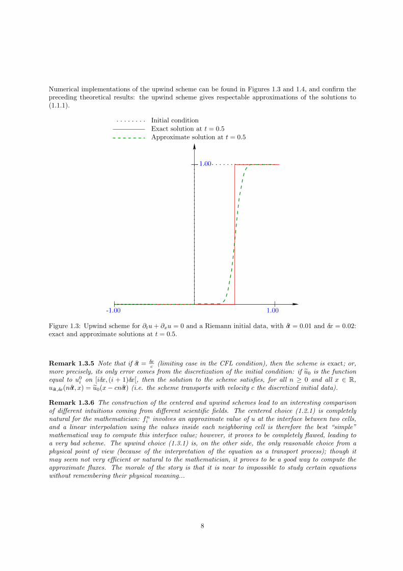
Numerical implementations of the upwind scheme can be found in Figures 1.3 and 1.4, and confirm thepreceding theoretical results: the upwind scheme gives respectable approximations of the solutions to(1.1.1).

-1.00 1.00

1.00

Approximate solution at t = 0.5Exact solution at t = 0.5Initial condition

Figure 1.3: Upwind scheme for ∂tu+ ∂xu = 0 and a Riemann initial data, with δt = 0.01 and δx = 0.02:exact and approximate solutions at t = 0.5.

Remark 1.3.5 Note that if δt = δxc (limiting case in the CFL condition), then the scheme is exact; or,

more precisely, its only error comes from the discretization of the initial condition: if u0 is the functionequal to u0i on [iδx, (i + 1)δx[, then the solution to the scheme satisfies, for all n ≥ 0 and all x ∈ R,uδt,δx(nδt, x) = u0(x− cnδt) (i.e. the scheme transports with velocity c the discretized initial data).

Remark 1.3.6 The construction of the centered and upwind schemes lead to an interesting comparisonof different intuitions coming from different scientific fields. The centered choice (1.2.1) is completelynatural for the mathematician: fni involves an approximate value of u at the interface between two cells,and a linear interpolation using the values inside each neighboring cell is therefore the best “simple”mathematical way to compute this interface value; however, it proves to be completely flawed, leading toa very bad scheme. The upwind choice (1.3.1) is, on the other side, the only reasonable choice from aphysical point of view (because of the interpretation of the equation as a transport process); though itmay seem not very efficient or natural to the mathematician, it proves to be a good way to compute theapproximate fluxes. The morale of the story is that it is near to impossible to study certain equationswithout remembering their physical meaning...

8

-1.00 1.00-0.50 0.50

-1.00

1.00

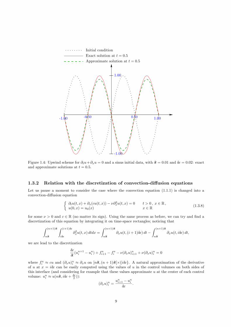
Exact solution at t = 0.5

Approximate solution at t = 0.5

Initial condition

Figure 1.4: Upwind scheme for ∂tu+∂xu = 0 and a sinus initial data, with δt = 0.01 and δx = 0.02: exactand approximate solutions at t = 0.5.

1.3.2 Relation with the discretization of convection-diffusion equations

Let us pause a moment to consider the case where the convection equation (1.1.1) is changed into aconvection-diffusion equation{

∂tu(t, x) + ∂x(cu(t, x))− ν∂2xu(t, x) = 0 t > 0 , x ∈ R ,u(0, x) = u0(x) x ∈ R (1.3.8)

for some ν > 0 and c ∈ R (no matter its sign). Using the same process as before, we can try and find adiscretization of this equation by integrating it on time-space rectangles; noticing that∫ (n+1)δt

nδt

∫ (i+1)δx

iδx

∂2xu(t, x) dtdx =

∫ (n+1)δt

nδt

∂xu(t, (i+ 1)δx) dt−∫ (n+1)δt

nδt

∂xu(t, iδx) dt,

we are lead to the discretization

δx

δt(un+1i − uni ) + fni+1 − fni − ν(∂xu)ni+1 + ν(∂xu)ni = 0

where fni ≈ cu and (∂xu)ni ≈ ∂xu on [nδt, (n + 1)δt[×{iδx}. A natural approximation of the derivativeof u at x = iδx can be easily computed using the values of u in the control volumes on both sides ofthis interface (and considering for example that these values approximate u at the center of each controlvolume: uni ≈ u(nδt, iδx+ δx

2 )):

(∂xu)ni =uni+1 − uni

δx.

9

Taking then a centered discretization for fni , we obtain the following discretization of the PDE in (1.3.8):

δx

δt(un+1i − uni ) + c

uni+1 − uni−12

− νuni+1 − uni

δx+ ν

uni − uni−1δx

= 0. (1.3.9)

What would it take for (1.3.9) to satisfy the maximum principle (which is valid for the PDE (1.3.8) itdiscretizes)? Let us make the same reasoning as in the proof of Proposition 1.3.1: from (1.3.9) we write

un+1i =

(1− 2ν

δt

δx2

)uni +

(νδt

δx2− c

2

δt

δx

)uni+1 +

(νδt

δx2+c

2

δt

δx

)uni−1.

The sum of the coefficients of uni−1, uni and uni+1 is equal to 1 and un+1i is thus a convex combination of

uni−1, uni and uni+1 provided that all these coefficients are non-negative, that is to say:

2νδt

δx2≤ 1 (1.3.10)

and|c|2δx ≤ ν. (1.3.11)

Remark 1.3.7 Condition (1.3.10) plays the role of the CFL condition, albeit involving a relation betweenthe discretization steps and the coefficient ν of the higher order term in (1.3.8) (i.e. the diffusion term);one can notice that this condition is much more restrictive than the CFL for the upwind discretizationof the transport equation: the time step must here be of order the square of the space step (hence a smallspace step imposes a much smaller time step: if the space step is divided by 10, the time step must bedivided by 100).

Remark 1.3.8 Although we have chosen a centered discretization for the convection term ∂x(cu), thepresence of the diffusion term allows to bound the approximate solution provided that (1.3.11) is satisfied;this condition (called the Peclet condition) states that, if the convection and diffusion coefficients arefixed, then a small enough space step is enough to control the convection term using the diffusion term.However, in many practical situations, ν can be quite small with respect to c and (1.3.11) then imposesa strong condition on δx.

Let us now come back to the upwind discretization (1.3.2) of (1.1.1) (we thus take c > 0), and let usrewrite it the following way:

δt

δx(un+1i − uni ) + c

uni+1 − uni−12

− cδx

2

uni+1 − uniδx

+cδx

2

uni − uni−1δx

= 0. (1.3.12)

Comparing this writing with (1.3.9), we notice that the upwind scheme for the linear pure convectionequation is identical to the discretization of a convection-diffusion equation using the centered scheme forthe convective part and the diffusion coefficient

ν =cδx

2

(of course, this comparison is formal and only holds at the discrete level since the diffusion coefficient ina true convection-diffusion equation cannot depend on some kind of “time step”).In other words, we can also say that the upwind discretization of a convection equation consists in adding

a small discrete diffusion term (namely − cδx2uni+1−u

ni

δx + cδx2

uni −u

ni−1

δx ≈ − cδx2∫ (i+1)δx

iδx∂2xu) to the centered

discretization of the same convection equation (compare (1.2.2) and (1.3.12)).One can also notice that, with this diffusion coefficient ν = cδx

2 (recall that c > 0 here), the Pecletcondition (1.3.11) of this formal discretization of a convection-diffusion equation is satisfied, and thatthe related CFL condition (1.3.10) is equivalent to the CFL condition (1.3.3) for the pure convectionequation.

10

1.3.3 About the time-implicit discretization

In (1.1.3), fni plays the role of an approximation of cu on [nδt, (n+ 1)δt[×{iδx}. We discussed the use ofapproximate values of u in the control volumes on either side of x = iδx to compute the numerical fluxfni ; however, we did not discuss the time at which these approximate values should be taken: t = nδt ort = (n+ 1)δt?In fact, right from the beginning we only considered that fni should be computed using (unj )j∈Z (i.e.only the values at time t = nδt); the advantage of this a priori choice is that it ensures that (1.1.3) isan equation allowing to simply and directly compute the approximate values at time t = (n+ 1)δt fromthe approximate values at time t = nδt. This is a quite natural expectation for evolution equations suchas (1.1.1) (which precisely tells how u evolves from a given initial state), but since fni is supposed toapproximate cu at x = iδx on the whole time interval [nδt, (n+ 1)δt[, a similar natural expectation wouldalso be to use the values at time t = (n+ 1)δt to compute fni .Still considering the case of an upwind scheme with c > 0, we could in particular choose, instead of(1.3.1),

fni = cun+1i−1 . (1.3.13)

The resulting scheme is

∀n ≥ 0 , ∀i ∈ Z :δx

δt(un+1i − uni ) + cun+1

i − cun+1i−1 = 0, (1.3.14)

to be completed with the discretization (1.1.4) of the initial condition. On the contrary to (1.3.2), (1.3.14)does not give a straightforward way to compute (un+1

i )i∈Z from (un)i∈Z; in fact, nothing ensures that,given (un)i∈Z, there exists (un+1

i )i∈Z which satisfies (1.3.14); put in another way: once (1.1.4) has given(u0i )i∈Z, will we even be able to find (let alone compute) (u1i )i∈Z from (1.3.14) ?

This scheme [(1.3.14),(1.1.4)] is called “implicit” because it only gives (if it exists) (un+1i )i∈Z from (uni )i∈Z

in an implicit way: solving (1.3.14) to compute (un+1i )i∈Z is not obvious. Implicit schemes are less easy

to use in practical, but they sometimes have very interesting properties. The reader familiar with theEuler discretizations of ODE can for example remember that, for equations of the kind y′(t) = −y(t),the explicit Euler scheme does not always preserve the positivity of the initial data (which is howeverpreserved by the ODE), whereas the implicit scheme ensures that the approximate solution stays positiveif the initial data is positive. For the conservation law (1.1.1), the implicit upwind scheme also has suchan interesting property: it satisfies the maximum principle whatever the values of the time and spacesteps (recall that the explicit scheme only satisfies this principle if the steps satisfy the CFL condition(1.3.3)).

Proposition 1.3.9 (Stability of the implicit upwind scheme) Let c > 0. For any δt > 0 and δx > 0, if(un)n≥0 , i∈Z satisfies [(1.3.14),(1.1.4)] and, for all n ≥ 0, supj∈Z |unj | < +∞, then

∀n ≥ 0 , ∀i ∈ Z : infj∈Z

unj ≤ un+1i ≤ sup

j∈Zunj . (1.3.15)

Proof of Proposition 1.3.9Let n ≥ 0 and assume first that there exists i0 ∈ Z such that un+1

i0= supj∈Z u

n+1j . The scheme (1.3.14)

gives

un+1i0− uni0 =

δt

δxc(un+1

i0−1 − un+1i0

). (1.3.16)

Now, by definition of i0 we have un+1i0−1 − u

n+1i0≤ 0 and thus supj∈Z u

n+1j = un+1

i0≤ uni0 ≤ supj∈Z u

nj ,

which proves the second inequality in (1.3.15).If such an i0 does not exist, then one can choose (ik)k≥1 such that un+1

ik→ supj∈Z u

n+1j as k →∞ (recall

that (un+1j )j∈Z is bounded by assumption) and deduce from (1.3.16) with ik instead of i0:

un+1ik≤ sup

j∈Zunj +

δt

δxc(supj∈Z

un+1j − un+1

ik).

11

Passing to the limit k →∞ gives back supj∈Z un+1j ≤ supj∈Z u

nj .

The first inequality in (1.3.15) can be deduced with a similar reasoning using either i0 such that un+1i0

=

infj∈Z un+1j or a sequence (ik)k≥1 such that un+1

ik→ infj∈Z u

n+1j as k →∞.

It remains to prove that there exists a bounded solution to [(1.3.2),(1.1.4)]. This solution indeed exists,and is unique (see e.g. the end of Section 2.5 for an idea of the proof, or the comments on the bibliographyat the end of the document).

Let us conclude this discussion on the implicit discretization by the following remark: in the equation∂tu + ∂x(cu) = 0, the same way the term ∂x(cu) models the convection of u at the velocity c along thespace direction, one could interpret ∂tu as the convection of u along the time direction with a velocity 1(evolution equations are nothing more than a transport toward the future). With such an interpretationin mind, our discussion on the discretization of convection terms would lead us to discretize ∂tu using anupwind choice; if we think of uni as an approximation on [nδt, (n+ 1)δt[×[iδx, (i+ 1)δx[ (and not only on[iδx, (i+ 1)δx[ at time t = nδt as our in previous idea) — which is coherent with the definition of uδt,δx inTheorem 1.3.3 — one would thus replace the term

δx

δt(un+1i − uni )

in (1.1.3) withδx

δt(uni − un−1i )

(approximating u at t = (n + 1)δt on [iδx, (i + 1)δx[ with its time-upwind value, that is to say its valueon [nδt, (n+ 1)δt[×[iδx, (i+ 1)δx[). With such a change, the upwind scheme (1.3.2), with the same choice(1.3.1) for fni as in the previous explicit discretization, becomes

δx

δt(uni − un−1i ) + cuni − cuni−1 = 0,

that is to say, up to a change of index n→ n+ 1, precisely the implicit upwind scheme (1.3.14).

Hence, the time-implicit discretization is nothing else than an upwind discretization of the temporalconvection term in the equation...

12

Chapter 2

Schemes for non-linear conservationlaws

2.1 Introduction

We now consider a non-linear scalar conservation law{∂tu(t, x) + ∂x(f(u(t, x))) = 0 t > 0 , x ∈ R ,u(0, x) = u0(x) x ∈ R (2.1.1)

with f : R → R locally Lipschitz-continuous and u0 ∈ L∞(R). Our aim is, once again, to constructa stable converging scheme to approximate the solution to (2.1.1); since this equation is non-linear, itswell-posedness requires the use of the notion of entropy solution (which we recall below) and we thereforehave to be careful to construct approximations to the (unique) entropy solution, and not another weaksolution.

Definition 2.1.1 (Entropy solution for (2.1.1)) An entropy solution to (2.1.1) is u ∈ L∞(]0,∞[×R)such that, for all κ ∈ R and all non-negative ϕ ∈ C∞c ([0,∞[×R),∫ ∞

0

∫R|u(t, x)− κ|∂tϕ(t, x)+(f(u(t, x)>κ)− f(u(t, x)⊥κ))∂xϕ(t, x) dtdx

+

∫R|u0(x)− κ|ϕ(0, x) dx ≥ 0 , (2.1.2)

where a>κ = max(a, κ) and a⊥κ = min(a, κ).

Remark 2.1.2 The usual definition of entropy solution makes use of general convex functions η : R→ Rand replaces |u(t, x) − κ| with η(u(t, x)) and f(u(t, x)>κ) − f(u(t, x)⊥κ) with φ(u(t, x)), where φ(s) =∫ s0η′(r)f ′(r) dr. Definition 2.1.1, using only Krushkov’s entropies η(s) = |s − κ|, is equivalent to the

general definition.

2.2 Monotone schemes

The principle of construction of a finite volume scheme for (2.1.1) is the same as in the linear case: wetake time and space steps δt and δx, and we integrate the equation on a cell [nδt, (n+ 1)δt[×[iδx, (i+ 1)δx[,obtaining ∫ (i+1)δx

iδx

u((n+ 1)δt, x) dx−∫ (i+1)δx

iδx

u(nδt, x) dx

13

+

∫ (n+1)δt

nδt

f(u(t, (i+ 1)δx)) dt−∫ (n+1)δt

nδt

f(u(t, iδx)) dt = 0.

If uni is an approximate value of u at time t = nδt on [iδx, (i+ 1)δx[ and fni is an approximation of f(u)on [nδt, (n+ 1)δt[ at x = iδx, dividing the preceding expression by δt, we are lead to consider the scheme

∀n ≥ 0 , ∀i ∈ Z :δx

δt(un+1i − uni ) + fni+1 − fni = 0. (2.2.1)

Assuming that fni is expressed in terms of (unj )j∈Z, completing (2.2.1) with the initial data

∀i ∈ Z : u0i =1

δx

∫ (i+1)δx

iδx

u0(x) dx , (2.2.2)

we obtain a scheme giving by induction the approximate values (uni )n≥0 , i∈Z. The hanging question istherefore to find an way to compute the approximation fni of f(u) in terms of the approximations (unj )j∈Zof u.

2.2.1 A first idea

Obviously, since it failed in the linear case (when f(u) = cu), there is little chance that the “natural”(for the mathematician) centered choice

fni =f(uni−1) + f(uni )

2(2.2.3)

works in general. However, following the reasoning in section 1.3.2 (linking, in the linear case, the upwindchoice with the discretization of an additional diffusion term), we can try and modify this centered choiceby adding some numerical diffusion.The centered discretization (2.2.3) leads to the scheme

∀n ≥ 0 , ∀i ∈ Z :δx

δt(un+1i − uni ) +

f(uni+1) + f(uni )

2−f(uni ) + f(uni−1)

2= 0.

Adding some diffusion terms as in (1.3.12), we would write

∀n ≥ 0 , ∀i ∈ Z :δx

δt(un+1i − uni ) +

f(uni+1) + f(uni )

2−f(uni ) + f(uni−1)

2−D(uni+1 − uni ) +D(uni − uni−1) = 0 (2.2.4)

with some D > 0 to be chosen so as to ensure the stability of the scheme. This scheme corresponds to(2.2.1) with

fni =f(uni−1) + f(uni )

2−D(uni − uni−1). (2.2.5)

A proper choice of D can be made by trying, as in the linear case, to transform (2.2.4) in order to expressun+1i as a convex combination of uni−1, uni and uni+1. We have

un+1i = uni −

δt

δx

f(uni+1) + f(uni )

2+δt

δx

f(uni ) + f(uni−1)

2

+Dδt

δx(uni+1 − uni )−D δt

δx(uni − uni−1)

= uni −δt

δx

f(uni+1)− f(uni )

2+δt

δx

f(uni−1)− f(uni )

2

+Dδt

δx(uni+1 − uni )−D δt

δx(uni − uni−1)

= uni −δt

δxαni (uni+1 − uni ) +

δt

δxβni (uni − uni−1)

+Dδt

δx(uni+1 − uni )−D δt

δx(uni − uni−1)

14

where αni =f(un

i+1)−f(uni )

2(uni+1−un

i )and βni =

f(uni−1)−f(u

ni )

2(uni −un

i−1)(if one or the other of the denominators vanishes, we

simply let αni = 0 or βni = 0). This leads to

un+1i = uni −

δt

δx(αni −D)(uni+1 − uni ) +

δt

δx(βni −D)(uni − uni−1)

=

(1 +

δt

δx(βni + αni − 2D)

)uni +

δt

δx(D − αni )uni+1 +

δt

δx(D − βni )uni−1

and un+1i is therefore a convex combination of uni−1, uni and uni+1 if

|αni | ≤ D and |βni | ≤ D (2.2.6)

and

|βni + αni − 2D| δtδx≤ 1. (2.2.7)

By construction, if Ln is the Lipschitz constant of f on [infi∈Z uni , supi∈Z u

ni ] then |αni | ≤ Ln

2 and |βni | ≤ Ln

2

and (2.2.6) and (2.2.7) are satisfied as soon as Ln

2 ≤ D and (Ln+2D) δtδx ≤ 1. It is easy to see by inductionon n that if we choose D, δt and δx such that

Lipu0(f)

2≤ D (2.2.8)

(with Lipu0(f) the Lipschitz constant of f on [infR u0, supR u0]) and

(Lipu0(f) + 2D)

δt

δx≤ 1 , (2.2.9)

then (2.2.6) and (2.2.7) are satisfied for all n ≥ 0 and the scheme [(2.2.1),(2.2.2),(2.2.5)] is stable: thecomputed approximate values all belong to [infR u0, supR u0].Equation (2.2.8) indicates how to take D in (2.2.5); we notice that D can be chosen only depending onf and u0. Equation (2.2.9) is the CFL condition associated with the scheme: as in the linear case, thetime step must not be to large with respect to the space step in order to obtain a stable approximation.This scheme is called the “modified” Lax-Friedrichs scheme (1).

2.2.2 General monotone schemes, L∞ stability

We would like to find more general ways to write the fni in (2.2.1) in terms of (unj )j∈Z. In a first approach,it seems reasonable to decide that fni will be computed using only uni−1 and uni (this was the case in thelinear upwind choice (1.3.1) and in the non-linear modified Lax-Friedrichs choice (2.2.5)), that is to say

fni = F (uni−1, uni ) with F : R× R→ R. (2.2.10)

The question is to find properties on F which ensure that [(2.2.1),(2.2.2),(2.2.10)] is a “good” scheme.

Obviously, there must be some kind of relation between F and f , since fni given by (2.2.10) is supposedto be an approximation of f(u) on [nδt, (n + 1)δt[ at x = iδx. A simple way to find such a relation is toconsider the case where the approximate values uni−1 and uni of u in the two cells neighboring x = iδxare identical: there is then no reason to imagine that an approximate value of u at x = iδx would differfrom this common value and thus, in this situation, we would like to have fni = f(uni−1) = f(uni ). Thisimposes

∀a ∈ R : F (a, a) = f(a).

1The original Lax-Friedrichs scheme consists in taking D = δx2δt

; its convergence however imposes an “inverse” CFL

condition δtδx≥ C (for some C > 0), therefore forcing δt and δx to have the same order (such a inverse CFL condition is not

required to obtain the convergence of the modified Lax-Friedrichs scheme, as we show below).

15

This property is satisfied by F (a, b) = f(a)+f(b)2 +D(a− b), the modified Lax-Friedrichs numerical flux.

As we already pointed out in the linear case and during the construction of the modified Lax-Friedrichsscheme, a crucial property of schemes is their stability. A way to ensure that F leads to a stable schemeis, once again, to check if (2.2.1) and (2.2.10) allow to see un+1

i as a convex combination of uni−1, uni anduni+1. We begin with

un+1i = uni −

δt

δxfni+1 +

δt

δxfni = uni −

δt

δxF (uni , u

ni+1) +

δt

δxF (uni−1, u

ni ) (2.2.11)

and, subtracting and adding F (uni , uni ) to the last two terms,

un+1i = uni −

δt

δx(F (uni , u

ni+1)− F (uni , u

ni )) +

δt

δx(F (uni−1, u

ni )− F (uni , u

ni ))

= uni +δt

δxani (uni+1 − uni ) +

δt

δxbni (uni−1 − uni ) (2.2.12)

where

ani = −F (uni , u

ni+1)− F (uni , u

ni )

uni+1 − uni(2.2.13)

and

bni =F (uni−1, u

ni )− F (uni , u

ni )

uni−1 − uni(2.2.14)

(as before, if one or the other denominator vanishes, so does the corresponding quantity ani or bni ). From(2.2.12) we obtain

un+1i =

(1− δt

δx(ani + bni )

)uni +

δt

δxani u

ni+1 +

δt

δxbni u

ni−1. (2.2.15)

The convex combination is achieved if

ani ≥ 0 , bni ≥ 0 andδt

δx(ani + bni ) ≤ 1. (2.2.16)

The non-negativity of ani and bni is ensured if we impose that F is non-decreasing with respect to itsfirst argument, and non-increasing with respect to its second argument. If we assume that F is locallyLipschitz-continuous with respect to each of its arguments then, denoting Ln1 and Ln2 the Lipschitzconstants with respect to its first and second variables on [infi∈Z u

ni , supi∈Z u

ni ]2, we have |ani | ≤ Ln1 and

|bni | ≤ Ln2 and the last condition in (2.2.16) is satisfied if δtδx (Ln1 + Ln2 ) ≤ 1.

The preceding reasoning leads us to the following general definition of a “good” way to compute theapproximate fluxes fni by a formula (2.2.10).

Definition 2.2.1 (Monotone numerical flux and monotone schemes) A monotone (upwind) numericalflux for (2.1.1) is a function F : R× R→ R which satisfies the following properties:

∀a ∈ [infR u0, supR u0] : F (a, a) = f(a) , (2.2.17)

F is Lipschitz-continuous with respect to each of its variables on [infR u0, supR u0]2 , (2.2.18)

on [infR u0, supR u0]2, F is non-decreasing with respect to its first variableand non-increasing with respect to its second variable.

(2.2.19)

A monotone (upwind) scheme is [(2.2.1),(2.2.2),(2.2.10)] with F a monotone (upwind) numerical flux,that is to say

∀n ≥ 0 , ∀i ∈ Z :δx

δt(un+1i − uni ) + F (uni , u

ni+1)− F (uni−1, u

ni ) = 0 ,

∀i ∈ Z : u0i =1

δx

∫ (i+1)δx

iδx

u0(x) dx.

(2.2.20)

16

Remark 2.2.2 We ask for properties of F only on [infR u0, supR u0]2 because, as stated in the followingproposition, under a suitable CFL condition all the approximate values (uni )n≥0 , i∈Z computed by thescheme stay in fact inside [infR u0, supR u0].

The following proposition, which establishes the stability of monotone schemes, is a simple consequence(by induction on n) of the above reasoning.

Proposition 2.2.3 (Stability of monotone schemes) Assume that F is a monotone numerical flux for(2.1.1) and denote by Lip1,u0

(F ) and Lip2,u0(F ) the Lipschitz constants of F with respect to its first and

second variables on [infR u0, supR u0]2. Then, under the CFL condition

δt

δx(Lip1,u0

(F ) + Lip2,u0(F )) ≤ 1, (2.2.21)

if (uni )n≥0 ,i∈Z satisfies the scheme (2.2.20) we have

∀n ≥ 0 ,∀i ∈ Z : infj∈Z

unj ≤ un+1i ≤ sup

j∈Zunj .

In particular, all the values (uni )n≥0 , i∈Z are between the infimum and supremum values of u0 and

supn≥0 , i∈Z

|uni | ≤ ||u0||L∞(R).

2.2.3 Examples of monotone fluxes, interpretation of the CFL condition

Here are three possible kinds of F satisfying (2.2.17)–(2.2.19).

1. F (a, b) = f(a)+f(b)2 +D(a− b) with D ≥ Lipu0

(f)

2 (recall that Lipu0(f) is the Lipschitz constant of

f on [infR u0, supR u0]). This is the modified Lax-Friedrichs numerical flux.

2. F (a, b) = f1(a) + f2(b), where f is written f(s) = f1(s) + f2(s) with f1 non-decreasing and f2non-increasing (both functions being locally Lipschitz-continuous). This is the splitting numerical

flux (2). The modified Lax-Friedrichs flux is a special case of splitting flux with f1(s) = f(s)2 +Ds

and f2(s) = f(s)2 −Ds.

3.

F (a, b) =

{min[a,b] f if a ≤ b ,max[b,a] f if a > b.

(2.2.22)

This is the Godunov numerical flux, which we now discuss in more depth.

Remark 2.2.4 For a linear flux f(s) = cs, the modified Lax-Friedrichs numerical flux with D =Lipu0

(f)

2 = c2 and the Godunov numerical flux give back the upwind choice (1.3.1).

Expression (2.2.22) is a simple and straightforward definition of the Godunov numerical flux, but this isnot the original way it has been constructed. The idea of the Godunov flux is the following: in order toconstruct an approximation fni = F (a, b) of f(u) on [nδt, (n+ 1)δt] at x = iδx when uni−1 = a and uni = b,consider the Riemann problem ∂tv + ∂x(f(v)) = 0 t > 0 , x ∈ R ,

v(0, x) =

{a = uni−1b = uni

if x < 0 ,if x > 0.

(2.2.23)

2Not to be confused with the “splitting method” sometimes used in numerical analysis, see Remark 2.5.1.

17

and let fni = F (a, b) = f(v(δt, 0)) (the solution v might not be pointwise well-defined at x = 0, but theflux f(v) always is). In other words, we let the scalar conservation law evolve from the Riemann initialdata defined by uni−1 and uni and take the value of the resulting flux at time t = δt at the interface x = iδx.It is known that the solution to (2.2.23) is self-similar and can therefore be written v(t, x) = v∗(x/t); theGodunov flux also can be defined by F (a, b) = f(v∗(0)).If f is convex (or concave), then there are simple expressions for v (depending on whether a ≤ b — vis then a rarefaction wave — or a > b — v is then a shock) and it is easy to check that the definitionof F (a, b) through (2.2.23) is identical to (2.2.22). This is also true for more general f , but less easy toverify.

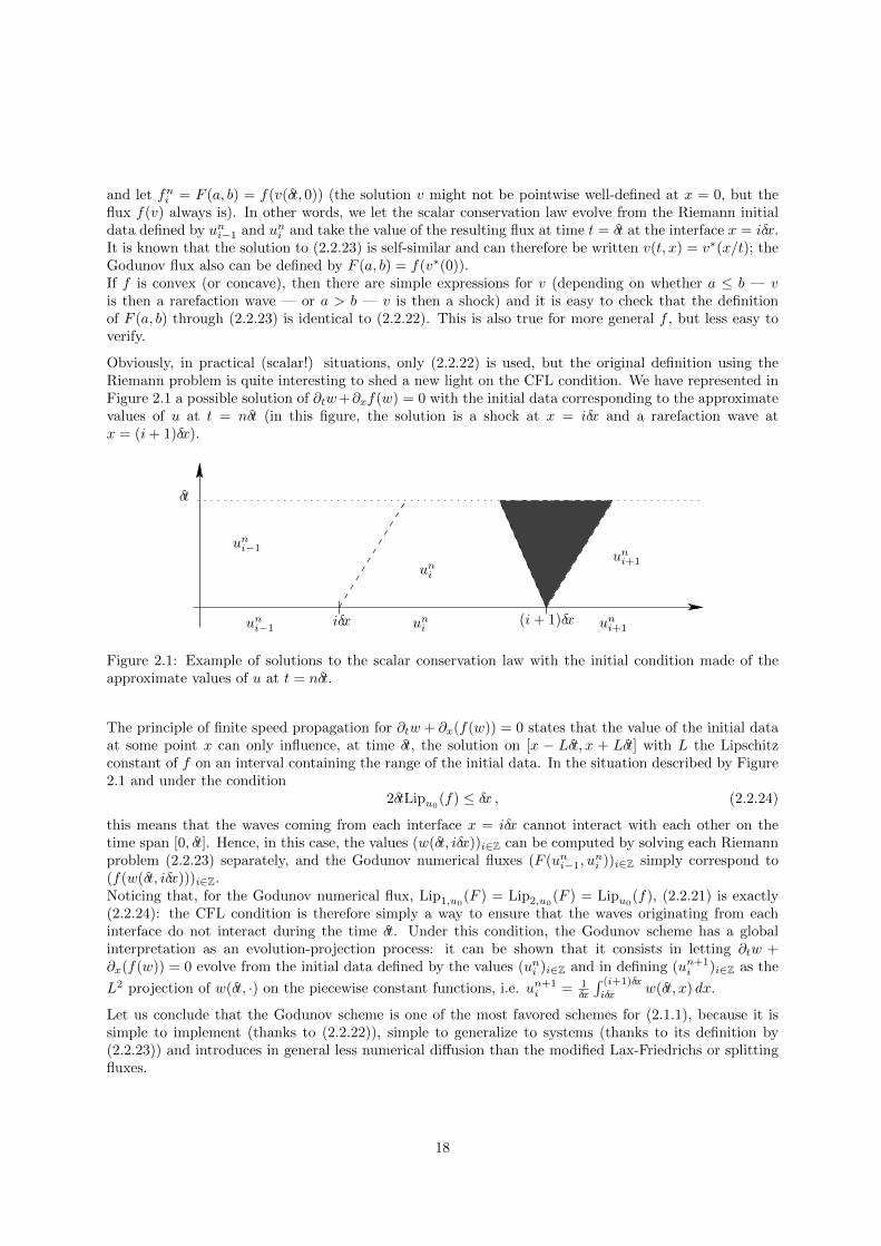
Obviously, in practical (scalar!) situations, only (2.2.22) is used, but the original definition using theRiemann problem is quite interesting to shed a new light on the CFL condition. We have represented inFigure 2.1 a possible solution of ∂tw+∂xf(w) = 0 with the initial data corresponding to the approximatevalues of u at t = nδt (in this figure, the solution is a shock at x = iδx and a rarefaction wave atx = (i+ 1)δx).

uni uni+1uni−1

uni−1

uniuni+1

iδx (i+ 1)δx

δt

Figure 2.1: Example of solutions to the scalar conservation law with the initial condition made of theapproximate values of u at t = nδt.

The principle of finite speed propagation for ∂tw + ∂x(f(w)) = 0 states that the value of the initial dataat some point x can only influence, at time δt, the solution on [x − Lδt, x + Lδt] with L the Lipschitzconstant of f on an interval containing the range of the initial data. In the situation described by Figure2.1 and under the condition

2δtLipu0(f) ≤ δx , (2.2.24)

this means that the waves coming from each interface x = iδx cannot interact with each other on thetime span [0, δt]. Hence, in this case, the values (w(δt, iδx))i∈Z can be computed by solving each Riemannproblem (2.2.23) separately, and the Godunov numerical fluxes (F (uni−1, u

ni ))i∈Z simply correspond to

(f(w(δt, iδx)))i∈Z.Noticing that, for the Godunov numerical flux, Lip1,u0

(F ) = Lip2,u0(F ) = Lipu0

(f), (2.2.21) is exactly(2.2.24): the CFL condition is therefore simply a way to ensure that the waves originating from eachinterface do not interact during the time δt. Under this condition, the Godunov scheme has a globalinterpretation as an evolution-projection process: it can be shown that it consists in letting ∂tw +∂x(f(w)) = 0 evolve from the initial data defined by the values (uni )i∈Z and in defining (un+1

i )i∈Z as the

L2 projection of w(δt, ·) on the piecewise constant functions, i.e. un+1i = 1

δx

∫ (i+1)δx

iδxw(δt, x) dx.

Let us conclude that the Godunov scheme is one of the most favored schemes for (2.1.1), because it issimple to implement (thanks to (2.2.22)), simple to generalize to systems (thanks to its definition by(2.2.23)) and introduces in general less numerical diffusion than the modified Lax-Friedrichs or splittingfluxes.

18

2.2.4 Numerical diffusion

The modified Lax-Friedrichs scheme has been constructing by adding some numerical diffusion to thecentered flux and, in fact, all monotone schemes can be seen as such.If F is a monotone numerical flux, (2.2.10) gives

fni =F (uni−1, u

ni−1) + F (uni , u

ni )

2+

1

2

(F (uni−1, u

ni )− F (uni−1, u

ni−1)

)+

1

2(F (uni−1, u

ni )− F (uni , u

ni ))

=f(uni−1) + f(uni )

2− g(uni−1, u

ni )(uni − uni−1) (2.2.25)

with

g(uni−1, uni ) = −

F (uni−1, uni )− F (uni−1, u

ni−1)

2(uni − uni−1)+F (uni−1, u

ni )− F (uni , u

ni )

2(uni−1 − uni ).

The monotony assumption (2.2.19) on F ensures that g(uni−1, uni ) ≥ 0 and (2.2.25) therefore shows that

fni indeed corresponds to a centered flux with the addition of a numerical diffusion term (compare with(2.2.5)), the coefficient of which depends on the unknowns at time step n.

2.3 Study of monotone schemes

We shall now prove that monotone schemes converge, as the time and space steps tend to 0 whilesatisfying the CFL condition, to (2.1.1). We have already proved in Proposition 2.2.3 an L∞ estimateon the approximate solution, which implies (up to a subsequence) the weak convergence of this solution;however, because of the non-linearity in (2.1.1), this weak convergence is not enough to conclude: wehave to prove stronger compactness properties on this solution, as well as some inequalities which ensurethat its possible limits are not only weak solutions to (2.1.1), but also entropy solutions.

2.3.1 BV estimates

The strong compactness property of the approximate solution is a consequence of the following BVestimates.

Proposition 2.3.1 (Space BV estimates) Assume that F is a monotone numerical flux for (2.1.1) andthat (2.2.21) holds. If (uni )n≥0 ,i∈Z satisfies the scheme (2.2.20), then

∀n ≥ 0 :∑i∈Z|un+1i − un+1

i−1 | ≤∑i∈Z|uni − uni−1|. (2.3.1)

In particular, if u0 ∈ BV (R) then

∀n ≥ 0 :∑i∈Z|uni − uni−1| ≤ |u0|BV (R) (2.3.2)

where |u0|BV (R) is the usual BV semi-norm of u0.

Remark 2.3.2 One can easily verify that∑i∈Z |uni −uni−1| is the total variation (the BV semi-norm) on

R of the piecewise constant function equal to uni on [iδx, (i+1)δx[ for all i ∈ Z; (2.3.1) therefore states thatthe space BV semi-norm of the approximate solution is non-increasing with respect to the time. Schemessatisfying this property are called Total Variation Decreasing (TVD).

Proof of Proposition 2.3.1

19

We use the expression (2.2.12) of the scheme to write

un+1i − un+1

i−1 = uni +δt

δxani (uni+1 − uni ) +

δt

δxbni (uni−1 − uni )

−uni−1 −δt

δxani−1(uni − uni−1)− δt

δxbni−1(uni−2 − uni−1)

=

(1− δt

δx(bni + ani−1)

)(uni − uni−1) +

δt

δxani (uni+1 − uni )− δt

δxbni−1(uni−2 − uni−1).

Under (2.2.17)–(2.2.19) and (2.2.21), since all the values (uni )i∈Z belong to [infR u0, supR u0] by Proposition2.2.3, we have 1− δt

δx (bni + ani−1) ≥ 0, ani ≥ 0 and bni−1 ≥ 0 (see (2.2.13) and (2.2.14)) and therefore

|un+1i − un+1

i−1 | ≤(

1− δt

δx(bni + ani−1)

)|uni − uni−1|+

δt

δxani |uni+1 − uni |+

δt

δxbni−1|uni−1 − uni−2|.

Summing this inequality on i ∈ Z and re-indexing the sums, we find∑i∈Z|un+1i − un+1

i−1 | ≤∑i∈Z

(1− δt

δx(bni + ani−1)

)|uni − uni−1|+

∑i∈Z

δt

δxani |uni+1 − uni |

+∑i∈Z

δt

δxbni−1|uni−1 − uni−2|

≤∑i∈Z

(1− δt

δx(bni + ani−1)

)|uni − uni−1|+

∑i∈Z

δt

δxani−1|uni − uni−1|

+∑i∈Z

δt

δxbni |uni − uni−1|

=∑i∈Z|uni − uni−1|

and (2.3.1) is proved.If u0 ∈ BV (R), one can check (3) that∑

i∈Z|u0i − u0i−1| ≤ |u0|BV (R)

and the proof is therefore complete by induction on n.

Proposition 2.3.3 (Time BV estimates) Assume that F is a monotone numerical flux for (2.1.1) andthat (2.2.21) holds. If (uni )n≥0 ,i∈Z satisfies the scheme (2.2.20) and u0 ∈ BV (R), then, for all T ≥ 0,

∑i∈Z

δx

[T/δt]∑n=0

|un+1i − uni | ≤ (T + δt)(Lip1,u0

(F ) + Lip2,u0(F ))|u0|BV (R)

where [T/δt] is the integer part of T/δt.

Remark 2.3.4 One can check that∑[T/δt]n=0 |u

n+1i − uni | is the BV semi-norm on [0, T ] of the piecewise

constant function equal to uni on [nδt, (n + 1)δt[ for all n ≥ 0. Proposition 2.3.3 therefore states a timeBV estimate on the approximate solution, which is quite expected once we have the space BV estimateof Proposition 2.3.1: indeed, for the continuous equation ∂tu+ ∂x(f(u)) = 0, a space BV estimate on ugives an estimate on ∂x(f(u)), which therefore translates into a similar estimate on ∂tu, i.e. a time BVestimate on u.

3Assume first that u0 ∈ C1 and write u0i − u0i−1 = 1δx

∫ (i+1)δxiδx (u0(x) − u0(x − δx)) dx =

∫ (i+1)δxiδx

∫ 10 u′0(x − sδx) dsdx,

so that∑i |u0i − u0i−1| ≤

∫ 10

∑i

∫ (i+1)δxiδx |u′0(x − sδx)| dx ds =

∫ 10

∫R |u′0(x − sδx)| dx ds = ||u′0||L1(R); the general case

u0 ∈ BV (R) is obtained by a density argument.

20

Proof of Proposition 2.3.3We have, from (2.2.12)–(2.2.14), (2.2.18) and the L∞ estimate in Proposition 2.2.3,

δx|un+1i − uni | ≤ δtLip2,u0

(F )|uni+1 − uni |+ δtLip1,u0(F )|uni−1 − uni |.

Summing on i ∈ Z and n = 0, . . . , [T/δt] (there is at most Tδt + 1 such n) and using Proposition 2.3.1 we

find ∑i∈Z

δx

[T/δt]∑n=0

|un+1i − uni | ≤ δt

(T

δt+ 1

)(Lip1,u0

(F ) + Lip2,u0(F ))|u0|BV (R)

and the proof is complete.

Corollary 2.3.5 Assume that F is a monotone numerical flux for (2.1.1) and that u0 ∈ BV (R). Then,for all T > 0, there exists C = C(T, F, u0) such that, if δx > 0 and δt ∈]0, 1[ satisfy (2.2.21) and(uni )n≥0 ,i∈Z satisfies the scheme (2.2.20),

|uδt,δx|BV ([0,T ]×R) ≤ C ,

where uδt,δx : R+×R→ R is the piecewise constant function equal to uni on [nδt, (n+ 1)δt[×[iδx, (i+ 1)δx[for all n ≥ 0 and i ∈ Z.

Proof of Corollary 2.3.5

We have |uδt,δx|BV ([0,T ]×R) ≤∫ T0|uδt,δx(t, ·)|BV (R) dt+

∫R |uδt,δx(·, x)|BV ([0,T ]) dx and the corollary follows

from Propositions 2.3.1, 2.3.3 and Remarks 2.3.2, 2.3.4.

2.3.2 Discrete entropy inequalities

The previous BV estimates and Helly’s theorem ensure the strong convergence of a subsequence ofapproximate solutions. However, in order to prove that the limit is not only a weak solution but theunique entropy solution to (2.1.1), we need some kind of discrete entropy inequalities (which, passing tothe limit, will give the strong entropy inequalities for the limit of the approximations).

Proposition 2.3.6 (Discrete entropy inequalities) Assume that F is a monotone numerical flux for(2.1.1) and that (2.2.21) holds. If (uni )n≥0 ,i∈Z satisfies the scheme (2.2.20) then, for all κ ∈ R,

∀n ≥ 0 , ∀i ∈ Z :δx

δt

[|un+1i − κ| − |uni − κ|

]+[F (uni >κ, uni+1>κ)− F (uni ⊥κ, uni+1⊥κ)

]−[F (uni−1>κ, uni >κ)− F (uni−1⊥κ, uni ⊥κ)

]≤ 0. (2.3.3)

Remark 2.3.7 Noticing that F (·>κ, ·>κ)−F (·⊥κ, ·⊥κ) satisfies (2.2.17) with f(·>κ)− f(·⊥κ) insteadof f , inequality (2.3.3) clearly is a discretization of

∂t|u− κ|+ ∂x (f(u>κ)− f(u⊥κ)) ≤ 0 ,

which is just another way of writing the entropy inequalities in Definition 2.1.1.

Proof of Proposition 2.3.6Let H(a, b, c) = b + δt

δxF (a, b) − δtδxF (b, c). The assumptions on F show that, under (2.2.21), H is non-

decreasing on [infR u0, supR u0]3 with respect to each of its variables, and we clearly have H(a, a, a) = a.By (2.2.11) we have un+1

i = H(uni−1, uni , u

ni+1) and the monotony properties of H therefore show that,

for all κ ∈ [infR u0, supR u0], since · ≤ ·>κ,

un+1i ≤ H(uni−1>κ, uni >κ, uni+1>κ). (2.3.4)

21

On the other hand, κ = H(κ, κ, κ) and therefore, still using the monotony of H,

κ ≤ H(uni−1>κ, uni >κ, uni+1>κ). (2.3.5)

We deduce from (2.3.4) and (2.3.5) that

un+1i >κ ≤ H(uni−1>κ, uni >κ, uni+1>κ). (2.3.6)

Similarly, it is easy to show that

un+1i ⊥κ ≥ H(uni−1⊥κ, uni ⊥κ, uni+1⊥κ). (2.3.7)

Subtracting (2.3.7) from (2.3.6), and using ·>κ− ·⊥κ = | · −κ| and the definition of H gives (2.3.3) whenκ ∈ [infR u0, supR u0]. If κ does not belong to this interval, then it is either greater or lower than all thevalues (uni )n≥0,i∈Z and one can check that the left-hand side of (2.3.3) then vanishes, thanks to (2.2.11).

Remark 2.3.8 This representation of the scheme as

un+1i = H(uni−1, u

ni , u

ni+1) (2.3.8)

(with H non-decreasing with respect to each of its variables and H(a, a, a) = a) has other applications;for example, one can prove Proposition 2.2.3 using this expression, by simply remarking that, if mn =infi∈Z u

ni and Mn = supi∈Z u

ni ,

mn = H(mn,mn,mn) ≤ H(uni−1, uni , u

ni+1) ≤ H(Mn,Mn,Mn) = Mn.

2.3.3 Convergence of the scheme

It is now quite easy to prove the convergence of the scheme.

Theorem 2.3.9 (Convergence of monotone schemes) Assume that F is a monotone numerical flux for(2.1.1) and that u0 ∈ BV (R). For δt > 0 and δx > 0, denote by uδt,δx the piecewise constant functionequal to uni on [nδt, (n + 1)δt[×[iδx, (i + 1)δx[, where (uni )n≥0 , i∈Z is the solution to the scheme (2.2.20).Then, as δt and δx tend to 0 while satisfying (2.2.21), uδt,δx converges to the entropy solution of (2.1.1)weakly-∗ in L∞(]0,∞[×R) and strongly in Lploc([0,∞[×R) for all p <∞ .

Remark 2.3.10 The condition u0 ∈ BV (R) is not mandatory, see Section 2.6.2.

Proof of Theorem 2.3.9By Proposition 2.2.3, Corollary 2.3.5 and Helly’s lemma (compact embedding of L1

loc ∩BVloc into L1loc),

we can extract a subsequence, still denoted uδt,δx, which converges to some u weakly-∗ in L∞(]0,∞[×R)and strongly in Lploc([0,∞[×R) for all p < ∞; if we prove that u is the entropy solution to (2.1.1), thenits uniqueness ensures that the whole sequence converges, which proves the theorem.Since u takes its values (as uδt,δx) between the infimum and supremum of u0, it is enough to prove (2.1.2)for κ also between these values; let such a κ, take ϕ ∈ C∞c ([0,∞[×R) non-negative and multiply each

equation of (2.3.3) by δtϕni with ϕni = 1δtδx

∫ (n+1)δt

nδt

∫ (i+1)δx

iδxϕ(t, x) dtdx. Summing on i and n (notice that

since ϕ has a compact support, these sums are in fact finite) and re-indexing some parts of these sums,we obtain

0 ≥∑n≥0

∑i∈Z

δx[|un+1i − κ| − |uni − κ|

]ϕni

+∑n≥0

δt∑i∈Z

[F (uni >κ, uni+1>κ)− F (uni ⊥κ, uni+1⊥κ)

]ϕni

22

−∑n≥0

δt∑i∈Z

[F (uni−1>κ, uni >κ)− F (uni−1⊥κ, uni ⊥κ)

]ϕni

≥∑n≥1

δt∑i∈Z

δx|uni − κ|ϕn−1i − ϕni

δt−∑i∈Z

δx|u0i − κ|ϕ0i

+∑n≥0

δt∑i∈Z

δx[F (uni−1>κ, uni >κ)− F (uni−1⊥κ, uni ⊥κ)

] ϕni−1 − ϕniδx

. (2.3.9)

We write

F (uni−1>κ, uni >κ)− F (uni−1⊥κ, uni ⊥κ) = F (uni−1>κ, uni >κ)− F (uni >κ, uni >κ)

+F (uni >κ, uni >κ)− F (uni ⊥κ, uni ⊥κ)

+F (uni ⊥κ, uni ⊥κ)− F (uni−1⊥κ, uni ⊥κ).

The consistency property (2.2.17) of F and its Lipschitz-continuity (2.2.18) (note that (uni )n≥0 , i∈Z andκ stay in [infR u0, supR u0]) imply, from (2.3.9) and using the regularity of ϕ and Proposition 2.3.1,

0 ≥∑n≥1

δt∑i∈Z

δx|uni − κ|ϕn−1i − ϕni

δt−∑i∈Z

δx|u0i − κ|ϕ0i

+∑n≥0

δt∑i∈Z

δx(f(uni >κ)− f(uni ⊥κ))ϕni − ϕni+1

δx+O

δx [T/δt]∑n=0

δt∑i∈Z|uni − uni−1|

0 ≥

∑n≥1

δt∑i∈Z

δx|uni − κ|ϕn−1i − ϕni

δt−∑i∈Z

δx|u0i − κ|ϕ0i

+∑n≥0

δt∑i∈Z

δx(f(uni >κ)− f(uni ⊥κ))ϕni − ϕni+1

δx+O(δx) , (2.3.10)

where T is some real number such that supp(ϕ) ⊂ [0, T ]× R.Define Φδt,δx : R+ × R → R, Ψδt,δx : R+ × R → R, Θδx : R → R and U0,κ

δx : R → R as the piecewiseconstant functions

Φδt,δx =ϕn−1i − ϕni

δton [nδt, (n+ 1)δt[×[iδx, (i+ 1)δx[ ,

Ψδt,δx =ϕni − ϕni+1

δton [nδt, (n+ 1)δt[×[iδx, (i+ 1)δx[ ,

Θδx = ϕ0i on [iδx, (i+ 1)δx[ ,

U0,κδx = |u0i − κ| on [iδx, (i+ 1)δx[ .

The regularity of ϕ and (2.2.2) show that, as δt and δx tend to 0,

Φδt,δx → −∂tϕ and Ψδt,δx → −∂xϕ uniformly on [0,∞[×R ,Θδx → ϕ(0, ·) uniformly on R and U0,κ

δx → |u0 − κ| in L1loc(R).

(2.3.11)

Note also that Φδt,δx, Ψδt,δx and Θδx vanish outside some compact sets not depending on δt or δx.Equation (2.3.10) can then be written

0 ≥∫ ∞0

∫R|uδt,δx − κ|Φδt,δx(t, x) dtdx−

∫RU0,κδx (x)Θδx(x) dx

+

∫ ∞0

∫R(f(uδt,δx(t, x)>κ)− f(uδt,δx(t, x)⊥κ))Ψδt,δx(t, x) dtdx+O(δx).

The strong convergence in L1loc([0,∞[×R) of uδt,δx and (2.3.11) allow to pass to the limit in this expression

and to conclude that u indeed satisfies (2.1.2), which completes the proof.

23

Remark 2.3.11 As it is usual in finite volume methods, the proof of convergence of the scheme relieson compactness estimates and does not require to have established the existence of a solution to the PDE;in fact, this study of convergence of the scheme gives, as a by-product, the existence of a solution to thecontinuous problem.

2.4 Some numerical results

Before presenting some numerical results, let us say a few words on the practical implementation. Eachtime step of the scheme (2.2.20) theoretically requires to compute an infinite number of values (un+1

i )i∈Z,which a computer obviously cannot do; one therefore has to compute only some of the unknowns, andthis can be achieved without loss thanks to the structure of the scheme.Equation (2.2.11) shows that un+1

i only depends on uni−1, uni and uni+1; hence, if we are interested in theapproximate solution at time t = Nδt (for some N ≥ 0) on the space interval [−Iδx, Iδx] (for some I ≥ 0),i.e. by (uNi )|i|≤I , we only need (uN−1i )|i|≤I+1, which in turn only requires (uN−2i )|i|≤I+2, etc., down to(u0i )|i|≤I+N .Therefore, in order to find the approximate solution at t = Nδt on [−Iδx, Iδx], the only values weneed to compute are uni for n = 0, . . . , N and |i| ≤ I + N − n; in particular, we only need to know(u0i )|i|≤I+N , i.e. u0 on [−(I + N)δx, (I + N)δx], in order to compute uδt,δx(Nδt, ·) on [−Iδx, Iδx]. Thisphenomenon is the discrete equivalent of the well-known “finite speed propagation property” of scalarconservation laws: this property states that the solution to (2.1.1) at time t = T on [−R,R] only dependson the initial data on [−R − Lipu0

(f)T,R + Lipu0(f)T ] (dependency cone). In the discrete setting, if

T = Nδt and R = Iδx, the approximate solution at t = T on [−R,R] depends on the initial data on[−R − δx

δt T,R + δxδt T ]; owing to the CFL condition (2.2.21), in the best case scenario this means that

we need u0 on [−R − (Lip1,u0(F ) + Lip2,u0

(F ))T,R + (Lip1,u0(F ) + Lip2,u0

(F ))T ]; in general, one hasLipi,u0

(F ) ≥ Lipu0(f) (with equality for the Godunov flux, for example): this means that the discrete

dependency cone is larger than the continuous dependency cone (its slope is, at best, twice as large).

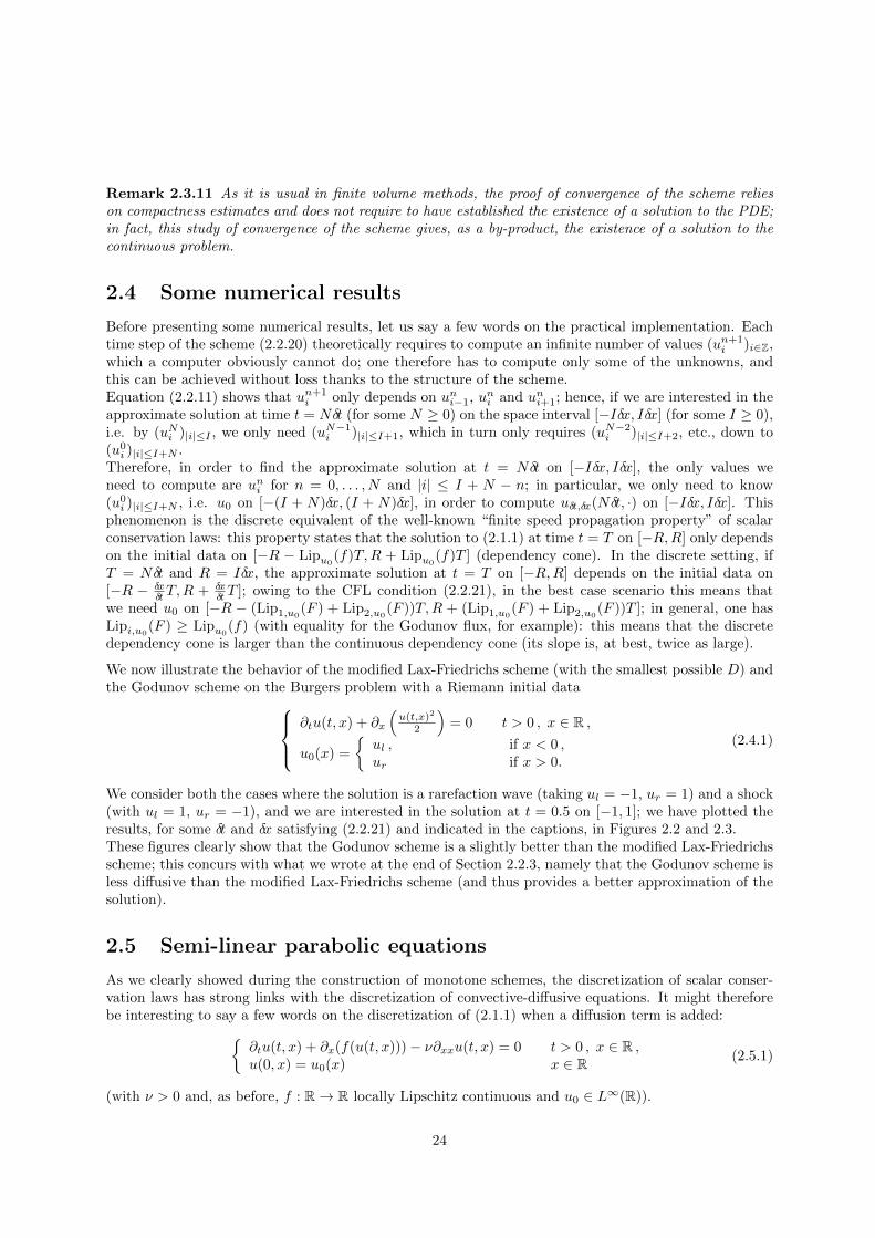
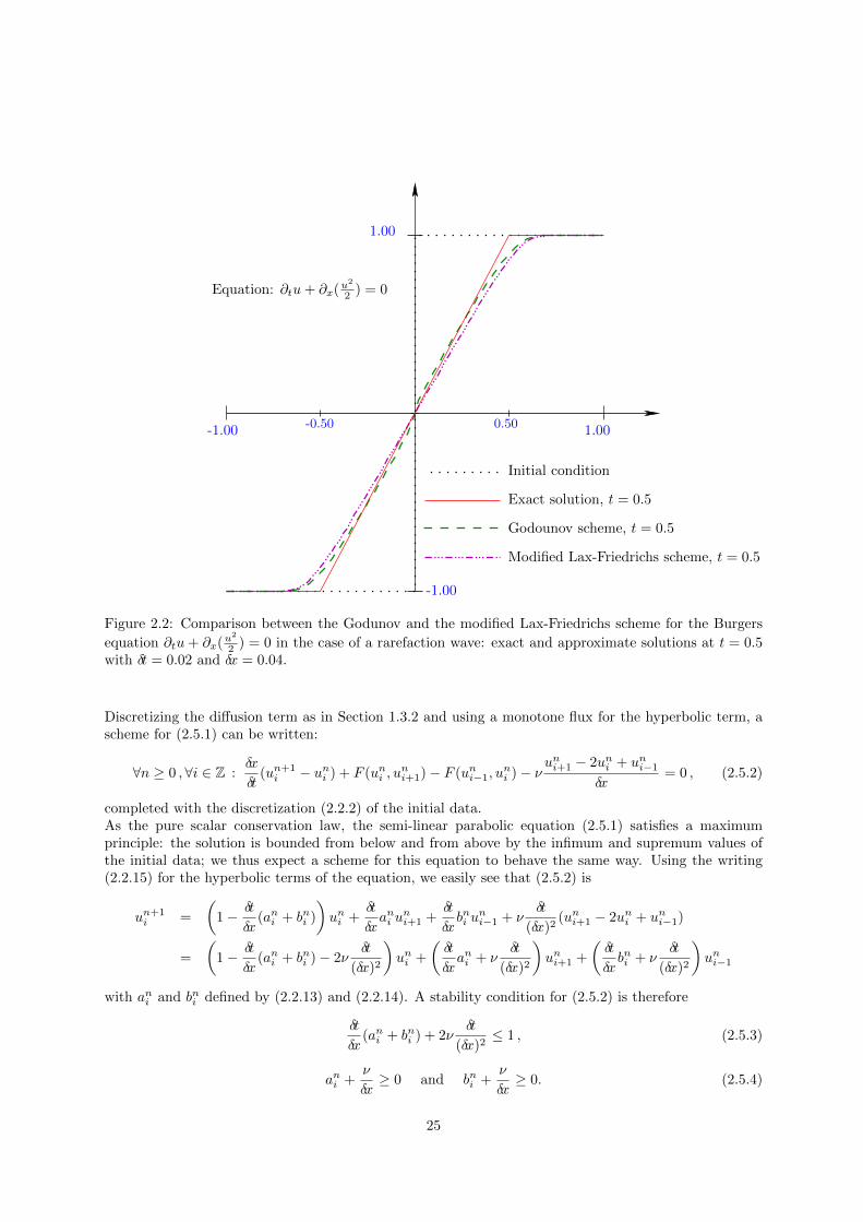
We now illustrate the behavior of the modified Lax-Friedrichs scheme (with the smallest possible D) andthe Godunov scheme on the Burgers problem with a Riemann initial data

∂tu(t, x) + ∂x

(u(t,x)2

2

)= 0 t > 0 , x ∈ R ,

u0(x) =

{ul ,ur

if x < 0 ,if x > 0.

(2.4.1)

We consider both the cases where the solution is a rarefaction wave (taking ul = −1, ur = 1) and a shock(with ul = 1, ur = −1), and we are interested in the solution at t = 0.5 on [−1, 1]; we have plotted theresults, for some δt and δx satisfying (2.2.21) and indicated in the captions, in Figures 2.2 and 2.3.These figures clearly show that the Godunov scheme is a slightly better than the modified Lax-Friedrichsscheme; this concurs with what we wrote at the end of Section 2.2.3, namely that the Godunov scheme isless diffusive than the modified Lax-Friedrichs scheme (and thus provides a better approximation of thesolution).

2.5 Semi-linear parabolic equations

As we clearly showed during the construction of monotone schemes, the discretization of scalar conser-vation laws has strong links with the discretization of convective-diffusive equations. It might thereforebe interesting to say a few words on the discretization of (2.1.1) when a diffusion term is added:{

∂tu(t, x) + ∂x(f(u(t, x)))− ν∂xxu(t, x) = 0 t > 0 , x ∈ R ,u(0, x) = u0(x) x ∈ R (2.5.1)

(with ν > 0 and, as before, f : R→ R locally Lipschitz continuous and u0 ∈ L∞(R)).

24

-1.00 1.00-0.50 0.50

-1.00

1.00

Equation: ∂tu+ ∂x(u2

2 ) = 0

Godounov scheme, t = 0.5

Modified Lax-Friedrichs scheme, t = 0.5

Exact solution, t = 0.5

Initial condition

Figure 2.2: Comparison between the Godunov and the modified Lax-Friedrichs scheme for the Burgers

equation ∂tu+ ∂x(u2

2 ) = 0 in the case of a rarefaction wave: exact and approximate solutions at t = 0.5with δt = 0.02 and δx = 0.04.

Discretizing the diffusion term as in Section 1.3.2 and using a monotone flux for the hyperbolic term, ascheme for (2.5.1) can be written:

∀n ≥ 0 ,∀i ∈ Z :δx

δt(un+1i − uni ) + F (uni , u

ni+1)− F (uni−1, u

ni )− ν

uni+1 − 2uni + uni−1δx

= 0 , (2.5.2)

completed with the discretization (2.2.2) of the initial data.As the pure scalar conservation law, the semi-linear parabolic equation (2.5.1) satisfies a maximumprinciple: the solution is bounded from below and from above by the infimum and supremum values ofthe initial data; we thus expect a scheme for this equation to behave the same way. Using the writing(2.2.15) for the hyperbolic terms of the equation, we easily see that (2.5.2) is

un+1i =

(1− δt

δx(ani + bni )

)uni +

δt

δxani u

ni+1 +

δt

δxbni u

ni−1 + ν

δt

(δx)2(uni+1 − 2uni + uni−1)

=

(1− δt

δx(ani + bni )− 2ν

δt

(δx)2

)uni +

(δt

δxani + ν

δt

(δx)2

)uni+1 +

(δt

δxbni + ν

δt

(δx)2

)uni−1

with ani and bni defined by (2.2.13) and (2.2.14). A stability condition for (2.5.2) is therefore

δt

δx(ani + bni ) + 2ν

δt

(δx)2≤ 1 , (2.5.3)

ani +ν

δx≥ 0 and bni +

ν

δx≥ 0. (2.5.4)

25

-1.00

1.00

1.00

Equation: ∂tu+ ∂x(u2

2 ) = 0Initial condition and exact solution

Godounov scheme

Modified Lax-Friedrichs scheme

-1.00

Figure 2.3: Comparison between the Godunov and the modified Lax-Friedrichs scheme for the Burgers

equation ∂tu + ∂x(u2

2 ) = 0 in the case of a shock: exact and approximate solutions at t = 0.5 withδt = 0.02 and δx = 0.04.

Equations (2.5.4) are always satisfied if F is a monotone flux (because ani ≥ 0 and bni ≥ 0 if (uni )i∈Zall belong to [infR u0, supR u0]), but they show that, in presence of a diffusion term, the monotonyassumptions on F can be relaxed: ani and bni do not necessarily need to be nonnegative, since they canbe compensated by the diffusion term. In particular, if

ν ≥ max(Lip1,u0(F ),Lip2,u0

(F ))δx (2.5.5)

then no monotony is required on F in order that (2.5.4) is satisfied; we already noticed this in thelinear case, and if F is the centered flux F (a, b) = 1

2 (f(a) + f(b)), (2.5.5) is the equivalent of the linearPeclet condition (1.3.11). In fact, one can understand from (2.5.4) exactly how to relax the monotonyassumptions on F . Define the “lower and upper Lipschitz constants” of F by

Lip−1,u0= sup

{(F (a, c)− F (b, c)

a− b

)−; (a, b, c) ∈ [inf

Ru0, sup

Ru0]3

}

and

Lip+2,u0

= sup

{(F (c, a)− F (c, b)

a− b

)+

; (a, b, c) ∈ [infRu0, sup

Ru0]3

}.

Since that ani ≥ −Lip+2,u0

(F ) and bni ≥ −Lip−1,u0(F ) (if (uni )i∈Z all belong to [infR u0, supR u0]), we see

that (2.5.4) is satisfied if we impose (2.5.5) with Lip−1,u0(F ) and Lip+

2,u0(F ) instead of Lip1,u0

(F ) andLip2,u0

(F ) (this gives a less restrictive condition, which is for example always satisfied in the case of a

monotone flux since we have then Lip−1,u0(F ) = Lip+

2,u0(F ) = 0).

26

In order to ensure (2.5.3), one basically has to impose

δt

δx(Lip1,u0

(F ) + Lip2,u0(F )) + 2ν

δt

(δx)2≤ 1 (2.5.6)

This condition, non-linear equivalent of (1.3.10) (4), shows that the diffusion term imposes a more re-strictive condition on the time and space steps than the hyperbolic term since it leads to a bound of thekind δt ≤ C(δx)2 (this has already been noticed in the linear case, see Remark 1.3.7). There is however away to avoid such a restrictive CFL condition: it consists in discretizing the diffusion term in a implicitway rather than an explicit one.

We write, instead of (2.5.2),

∀n ≥ 0 ,∀i ∈ Z :δx

δt(un+1i − uni ) + F (uni , u

ni+1)− F (uni−1, u

ni )− ν

un+1i+1 − 2un+1

i + un+1i−1

δx= 0. (2.5.7)

In order to study the stability of this semi-implicit scheme (the hyperbolic term is discretized in a explicitway, the diffusive term in an implicit way), we define

vni = uni −δt

δxF (uni , u

ni+1) +

δt

δxF (uni−1, u

ni ) (2.5.8)

and we notice that, under the usual hyperbolic CFL condition (2.2.21) (not involving (δx)2), if (uni )i∈Zall belong to [infR u0, supR u0] then the values (vni )i∈Z also belong to this interval, since these are simplythe values computed by the monotone scheme defined by F for the pure hyperbolic scalar conservationlaw (see (2.2.11)). Assume now that (uni )i∈Z are given real numbers in [infR u0, supR u0] and that thereexists a bounded sequence (un+1

i )i∈Z satisfying (2.5.7). Then

un+1i + ν

δt

(δx)2(un+1i − un+1

i+1 ) + νδt

(δx)2(un+1i − un+1

i−1 ) = vni (2.5.9)

and, taking (ik)k≥0 a sequence such that un+1ik→ supj∈Z u

n+1j and applying (2.5.9) to i = ik, we find

un+1ik

+ νδt

(δx)2(un+1ik− sup

j∈Z(un+1j )) + ν

δt

(δx)2(un+1ik− sup

j∈Z(un+1j )) ≤ sup

j∈Zvnj ≤ sup

Ru0.

Passing then to the limit k → ∞, we infer supj∈Z un+1j ≤ supR u0; similarly, we could show that

infj∈Z un+1j ≥ infR u0. This shows that the semi-implicit scheme (2.5.7) satisfies the maximum prin-

ciple (and is therefore stable) under the same CFL (2.2.21) as in the absence of a diffusion term; thisCFL is always less restrictive than (2.5.6), and much more so in the case of small space steps.There however remains the question of the existence, given (uni )i∈Z, of (un+1

i )i∈Z satisfying (2.5.7); onthe contrary to the case of the fully explicit scheme (2.5.2), this existence is not obvious. However, once apriori estimates on the possible solution (un+1

i )i∈Z have been obtained, one can apply classical techniqueswhich ensure the existence of this solution. Here, this would for example consist in cutting (2.5.7) inorder to consider only a finite number of equations, say for |i| ≤ I, to notice that the preceding a prioriestimates still holds for this finite-dimensional system and therefore ensure the existence and uniquenessof its solution, and to pass to the limit I → ∞ (still using the estimates on the solution) to obtain asolution to the full system (2.5.7); it is also possible to prove that this solution is unique.

Remark 2.5.1 As we have noticed, (vni )i∈Z defined by (2.5.8) is computed, from (uni )i∈Z, by applyingone time iteration of the monotone scheme for the pure hyperbolic conservation law (2.1.1). One can alsonotice that (2.5.9) consists in computing (un+1

i )i∈Z from (vni )i∈Z by applying one time iteration of the

4The term δtδx

(Lip1,u0(F ) + Lip2,u0

) does not appear in (1.3.10) because, in the linear case, one has ani + bni = 0.

27

scheme for the pure diffusion equation (i.e. (2.5.1) with f = 0). Each time iteration of the semi-implicitscheme (2.5.7) for

∂tu+ ∂x(f(u))− ν∂xxu = 0 (2.5.10)

therefore appears as the successive application of one time iteration of a scheme for

∂tu+ ∂x(f(u)) = 0

and one time iteration of a scheme for∂tu− ν∂xxu = 0.

This technique, which consists in cutting the evolution of (2.5.10) in two equations, is known in numericalanalysis as the splitting method.

2.6 Two concluding remarks

2.6.1 Implicit discretization of the fluxes

As in the linear case, another natural choice of flux discretization in (2.2.1) is to use an implicit form,replacing (2.2.10) with

fni = F (un+1i−1 , u

n+1i ). (2.6.1)

One can then prove that, if F is a monotone numerical flux, the resulting scheme [(2.2.1),(2.2.2),(2.6.1)]is L∞ stable without any CFL assumption. Indeed, it leads to

∀n ≥ 0 , ∀i ∈ Z : uni = un+1i +

δt

δxF (un+1

i , un+1i+1 )− δt

δxF (un+1

i−1 , un+1i ) =: G(un+1

i−1 , un+1i , un+1

i+1 ) (2.6.2)

with, on [infR u0, supR u0]3, G non-increasing with respect to its first and third variables, and non-decreasing with respect to its second variable and G(a, a, a) = a; assuming that there exists a solution(un+1i )i∈Z ∈ [infR u0, supR u0]Z to (2.6.2) and taking i such that un+1

i = supj∈Z un+1j (or, if such an i does

not exist, a sequence (ik)k≥0 such that un+1ik→ supj∈Z u

n+1j as in Section 2.5), we have

supj∈Z

unj ≥ G(un+1i−1 , u

n+1i , un+1

i+1 ) ≥ G(un+1i , un+1

i , un+1i ) = un+1

i = supj∈Z

un+1j .

Similarly, we would show that infj∈Z unj ≤ infj∈Z u

n+1j . These a priori estimates allow to prove the

existence of a solution (un+1i )i∈Z ∈ [infR u0, supR u0]Z to the scheme (2.6.2).

Implicit schemes for scalar conservation laws (2.1.1) are however not as used as for diffusion equations(2.5.1), because the resulting system (2.6.2) to solve is non-linear, and the study of MUSCL methods (seeChapter 3) for the implicit discretization is not obvious.

2.6.2 Convergence without BV estimates

We proved the convergence of the monotone scheme for (2.1.1) under the assumption that the initialdata has a bounded variation (see Theorem 2.3.9); the BV assumption has been used to obtain thecompactness of the approximate solution, and to prove that the error term in (2.3.10) tends to 0 withthe space step.It is however possible to prove the convergence of the scheme without any assumption on u0 besides thefact that it belongs to L∞(R). An idea is, instead of trying to prove an a priori compactness property onthe approximate solution, to use Young’s measure theory in order to pass to the limit (in a “non-linearweak-∗” sense) in the non-linear terms of the entropy inequalities (2.3.3); the resulting limit is no longera function of (t, x), but a Young measure (roughly speaking, a family of probability measures (νt,x)t,x onR), which can be represented by its repartition function (a function of (t, x, α), where α is an additional

28

variable) called “entropy process solution”. One then shows a strong uniqueness property for this entropyprocess solution, which proves that it does not depend on α and is therefore a classical entropy solution(a function of (t, x)); this gives, as an a posteriori by-product, the strong convergence of the approximatesolutions toward this entropy solution.

Notice however that, even if one does not need a BV estimate on the approximate solution to obtain anon-linear weak-∗ compactness property on it, some kind of “weak BV estimate” is required in order tocontrol the error term in (2.3.10). This estimate is written∑

i∈Z|uni − uni−1| ≤

C√δx

(compare with (2.3.2)); the error term in (2.3.10) is then not O(δx) but O(√δx) and therefore still vanishes

as δx→ 0.

29

Chapter 3

MUSCL methods

3.1 Position of the problem, principle of MUSCL schemes

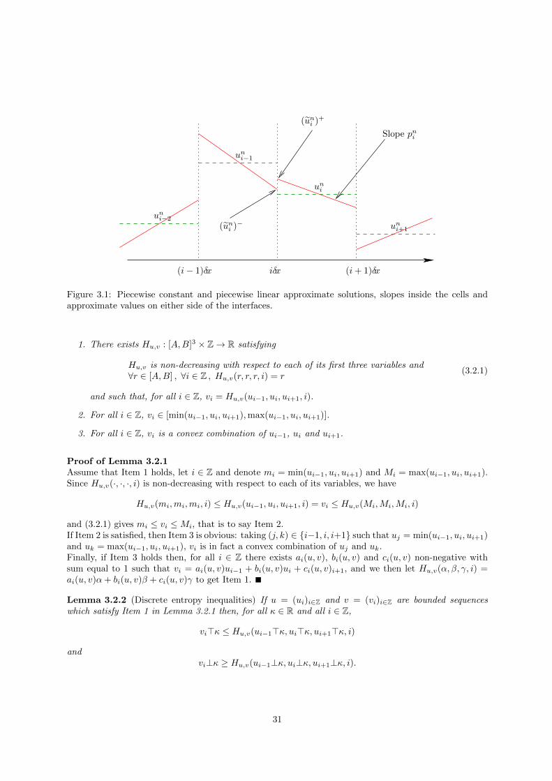
The finite volume method presented in Chapter 2 approximates the solution with functions which areconstant on each space cell; in particular, the numerical fluxes computed at an interface x = iδx usesthe two values uni−1 and uni inside the neighboring cells: if one (quite naturally) considers these values aspointwise approximations of the solution at the center of each cell, this means that the interface valuesare computed using values at a distance δx/2 of the said interface. The order of the resulting scheme istherefore not very high (the consistency error on the fluxes is at best a O(δx)) and, as can be seen inFigure 2.2 and 2.3, the resulting approximations, though correct, are not very good, especially near thepoints where the exact solution is not smooth. We would like to present here some methods which allowto increase the quality of monotone schemes.

The MUSCL methods (Monotone Upwind Scheme for Conservation Laws) consist, instead of consider-ing piecewise constant approximation of the solution, in using piecewise linear (discontinuous) approx-

imations. uni is then considered as the approximate value at the center iδx+(i+1)δx2 of the space cell

[iδx, (i+ 1)δx[ and slopes (pni )i∈Z are computed inside each cell, which allows to obtain approximate val-ues (uni )− = uni−1 + pni−1

δx2 and (uni )+ = uni − pni δx2 of the solution on the left and right of each interface

x = iδx (see Figure 3.1). These values are (hopefully) better approximations of u at x = iδx than uni−1and uni , and can then be used in (2.2.10) to compute the approximate fluxes:

fni = F ((uni )−, (uni )+) = F

(uni−1 + pni−1

δx

2, uni − pni

δx

2

). (3.1.1)

The resulting scheme [(2.2.1),(3.1.1)] is

un+1i = uni +

δt

δxF

(uni−1 + pni−1

δx

2, uni − pni

δx

2

)− δt

δxF

(uni + pni

δx

2, uni+1 − pni+1

δx

2

), (3.1.2)

completed with the discretization of the initial condition (2.2.2). The only remaining task is to find away to compute the fluxes pni so that (3.1.2) gives rise to a stable scheme.

3.2 General stability and entropy lemmas

Let us first state two general lemmas for schemes written under a slightly more general form than (2.3.8).The first lemma gives a very general description of stable schemes, and the second lemma shows thatsuch schemes satisfy the entropy inequalities.

Lemma 3.2.1 (General stability result) Let u = (ui)i∈Z and v = (vi)i∈Z be two bounded sequences,A = infi∈Z ui and B = supi∈Z ui. The following properties are equivalent:

30

(i+ 1)δx

uni−2

uni−1

uni

uni+1

(uni )+

Slope pni

(uni )−

(i− 1)δx iδx

Figure 3.1: Piecewise constant and piecewise linear approximate solutions, slopes inside the cells andapproximate values on either side of the interfaces.

1. There exists Hu,v : [A,B]3 × Z→ R satisfying

Hu,v is non-decreasing with respect to each of its first three variables and∀r ∈ [A,B] , ∀i ∈ Z , Hu,v(r, r, r, i) = r

(3.2.1)

and such that, for all i ∈ Z, vi = Hu,v(ui−1, ui, ui+1, i).

2. For all i ∈ Z, vi ∈ [min(ui−1, ui, ui+1),max(ui−1, ui, ui+1)].

3. For all i ∈ Z, vi is a convex combination of ui−1, ui and ui+1.

Proof of Lemma 3.2.1Assume that Item 1 holds, let i ∈ Z and denote mi = min(ui−1, ui, ui+1) and Mi = max(ui−1, ui, ui+1).Since Hu,v(·, ·, ·, i) is non-decreasing with respect to each of its variables, we have

Hu,v(mi,mi,mi, i) ≤ Hu,v(ui−1, ui, ui+1, i) = vi ≤ Hu,v(Mi,Mi,Mi, i)

and (3.2.1) gives mi ≤ vi ≤Mi, that is to say Item 2.If Item 2 is satisfied, then Item 3 is obvious: taking (j, k) ∈ {i−1, i, i+1} such that uj = min(ui−1, ui, ui+1)and uk = max(ui−1, ui, ui+1), vi is in fact a convex combination of uj and uk.Finally, if Item 3 holds then, for all i ∈ Z there exists ai(u, v), bi(u, v) and ci(u, v) non-negative withsum equal to 1 such that vi = ai(u, v)ui−1 + bi(u, v)ui + ci(u, v)i+1, and we then let Hu,v(α, β, γ, i) =ai(u, v)α+ bi(u, v)β + ci(u, v)γ to get Item 1.

Lemma 3.2.2 (Discrete entropy inequalities) If u = (ui)i∈Z and v = (vi)i∈Z are bounded sequenceswhich satisfy Item 1 in Lemma 3.2.1 then, for all κ ∈ R and all i ∈ Z,

vi>κ ≤ Hu,v(ui−1>κ, ui>κ, ui+1>κ, i)

andvi⊥κ ≥ Hu,v(ui−1⊥κ, ui⊥κ, ui+1⊥κ, i).

31

Proof of Lemma 3.2.2The proof is the same as the proof of Proposition 2.3.6: (3.2.1) gives

vi = Hu,v(ui−1, ui, ui+1, i) ≤ Hu,v(ui−1>κ, ui>κ, ui+1>κ, i)

andκ = Hu,v(κ, κ, κ, i) ≤ Hu,v(ui−1>κ, ui>κ, ui+1>κ, i).

Taking the supremum of these two inequalities gives the first inequality in the lemma, and a similarreasoning allows to prove the second inequality.

3.3 Example of a MUSCL scheme

We have to find ways to compute slopes pni , using (unj )j∈Z, which ensure that the solution to (3.1.2)satisfies the maximum principle. It is quite simple to compute slopes inside the cells, taking for example

pni =uni+1−u

ni−1

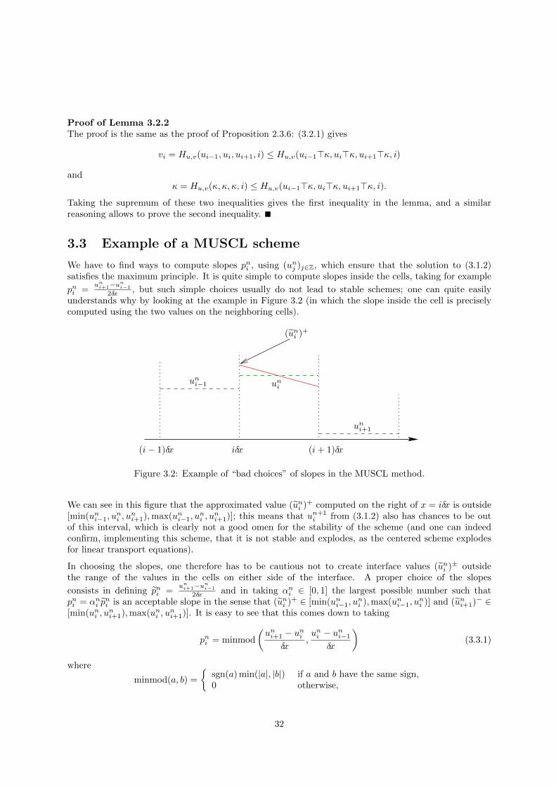
2δx , but such simple choices usually do not lead to stable schemes; one can quite easilyunderstands why by looking at the example in Figure 3.2 (in which the slope inside the cell is preciselycomputed using the two values on the neighboring cells).

uni+1

uni−1 uni

(uni )+

(i− 1)δx iδx (i+ 1)δx

Figure 3.2: Example of “bad choices” of slopes in the MUSCL method.

We can see in this figure that the approximated value (uni )+ computed on the right of x = iδx is outside[min(uni−1, u

ni , u

ni+1),max(uni−1, u

ni , u

ni+1)]; this means that un+1

i from (3.1.2) also has chances to be outof this interval, which is clearly not a good omen for the stability of the scheme (and one can indeedconfirm, implementing this scheme, that it is not stable and explodes, as the centered scheme explodesfor linear transport equations).

In choosing the slopes, one therefore has to be cautious not to create interface values (uni )± outsidethe range of the values in the cells on either side of the interface. A proper choice of the slopes

consists in defining pni =uni+1−u

ni−1

2δx and in taking αni ∈ [0, 1] the largest possible number such thatpni = αni p

ni is an acceptable slope in the sense that (uni )+ ∈ [min(uni−1, u

ni ),max(uni−1, u

ni )] and (uni+1)− ∈

[min(uni , uni+1),max(uni , u

ni+1)]. It is easy to see that this comes down to taking

pni = minmod

(uni+1 − uni

δx,uni − uni−1

δx

)(3.3.1)

where

minmod(a, b) =

{sgn(a) min(|a|, |b|) if a and b have the same sign,0 otherwise,

32

i.e. pni vanishes if the two slopes computed with (uni−1, uni ) and (uni , u

ni+1) have different signs, and is the

smallest (in absolute value) possible slope between those two if they have the same sign.

Let us look at the stability and entropy inequalities for the scheme [(3.1.2),(3.3.1),(2.2.2)] thus obtained,beginning with a few simple properties.

Lemma 3.3.1 Let [a, b] be the set of numbers between a and b, whatever the order of a and b, and 1Athe characteristic function of A ⊂ R. The following properties hold:

(a, b)→ minmod(a, b) is non-decreasing with respect to each of its variables, (3.3.2)

Defining mni =

uni−1+u

ni+1

2 , we have pniδx2 = 1[un

i−1,mni [

(uni )uni −u

ni−1

2 + 1[mni ,u

ni+1]

(uni )uni+1−u

ni

2 , (3.3.3)

(uni−1, uni , u

ni+1)→ uni + pni

δx2 is non-increasing with respect to uni−1,

non-decreasing with respect to uni and uni+1 and:a) Lipschitz-continuous with constant 1.5 with respect to uni if uni ∈ [uni−1,m

ni ],

b) Lipschitz-continuous with constant 0.5 with respect to uni if uni ∈ [mni , u

ni+1],

c) Lipschitz-continuous with constant 1 with respect to uni elsewhere,

(3.3.4)

(uni−1, uni , u

ni+1)→ uni − pni δx2 is non-increasing with respect to uni+1,

non-decreasing with respect to uni−1 and uni and:a) Lipschitz-continuous with constant 0.5 with respect to uni if uni ∈ [uni−1,m

ni ],

b) Lipschitz-continuous with constant 1.5 with respect to uni if uni ∈ [mni , u

ni+1],

c) Lipschitz-continuous with constant 1 with respect to uni elsewhere.

(3.3.5)

Proof of Lemma 3.3.1We deduce (3.3.2) from the symmetry of minmod and a study of two cases: if b is non-negative,minmod(a, b) = 0 for a ≤ 0, = a for 0 ≤ a ≤ b and = b for a > b and, if b is non-positive, minmod(a, b) = 0for a ≥ 0, = a for b ≤ a ≤ 0 and = b for b < a.Property (3.3.3) can be checked by studying all possible situations: uni 6∈ [uni−1, u

ni+1] (the two slopes used

to define pni then have opposite signs, and pni = 0), uni ∈ [uni−1,mni [ (we have then |uni −uni−1| ≤ |uni+1−uni |)

and uni ∈ [mni , u

ni+1] (in which case |uni − uni−1| ≥ |uni+1 − uni |).

Both (3.3.4) and (3.3.5) are consequences of (3.3.1) and (3.3.2) (which show that pni is non-decreasingwith respect to uni+1 and non-increasing with respect to uni−1) and of (3.3.3) (for the properties concerninguni ).

Equation (3.1.2) can be written

un+1i = uni +

δt

δxF(ci1(uni−1, u

ni ), di1(uni , u

ni+1)

)− δt

δxF(di2(uni , u

ni−1), ci2(uni , u

ni+1)

)(3.3.6)

where

ci1(uni−1, uni ) = uni−1 + pni−1

δx

2, ci2(uni , u

ni+1) = uni+1 − pni+1

δx

2,

di1(uni , uni+1) = uni − pni

δx

2and di2(uni , u

ni−1) = uni + pni

δx

2

depend on other (unj )j∈Z than the ones explicitly stated, but satisfy the following properties (whateverthe values of these other (unj )j∈Z):

• ci1 and ci2 are non-decreasing with respect to their two variables,

• di1 and di2 are non-decreasing with respect to their first variable and non-increasing with respect totheir second variable,

33

• for all (uni−1, uni , u

ni+1),

a) di1 and di2 are Lipschitz-continuous with respective constants 0.5 and 1.5with respect to uni if uni ∈ [uni−1,m

ni ],

b) di1 and di2 are Lipschitz-continuous with respective constant 1.5 and 0.5with respect to uni if uni ∈ [mn

i , uni+1],

c) di1 and di2 are Lipschitz-continuous with constant 1 with respect to uni elsewhere,

• ci1(s, s) = ci2(s, s) = di1(s, s) = di2(s, s) = s for all s ∈ R

(this last property comes from minmod(0, r) = minmod(r, 0) = 0 for all r ∈ R). From these remarks andthe monotony (2.2.19) of F , we see that the right-hand side of (3.3.6) is non-decreasing with respect touni , when all values (unj )j∈Z are inside [infR u0, supR u0], as soon as

δt

δxmax

[0.5Lip2,u0

(F ) + 1.5Lip1,u0(F ) ; 1.5Lip2,u0

(F ) + 0.5Lip1,u0(F ) ;

Lip2,u0(F ) + Lip1,u0

(F )]≤ 1. (3.3.7)

Under this assumption, the monotony and consistency properties of F , ci1, ci2, di1 and di2 thus prove that(3.3.6) can be written

un+1i = Hun,un+1(uni−1, u

ni , u

ni+1, i)

with un+1 = (un+1j )j∈Z, un = (unj )j∈Z and Hun,un+1 satisfying (3.2.1) (the first three variables of Hun,un+1

are the uni−1, uni , uni+1 explicitly appearing in the right-hand side of (3.3.6)). The L∞ stability (in fact themaximum principle) and the entropy inequalities for the MUSCL scheme [(3.1.2),(3.3.1),(2.2.2)] followthen from Lemmas 3.2.1 and 3.2.2.

Let us conclude by noting that (3.3.7) is the CFL condition associated with the 5-points (1) MUSCLmethod [(3.1.2),(3.3.1),(2.2.2)], and that it is equivalent to

δt

δxmax

[1.5Lip1,u0

(F ) + 0.5Lip2,u0(F ) ; 0.5Lip1,u0

(F ) + 1.5Lip2,u0(F )]≤ 1. (3.3.8)

This condition for the MUSCL implementation of the chosen monotone scheme is slightly more demandingthan the initial CFL (2.2.21), but not very much (it is the same if Lip1,u0

(F ) = Lip2,u0(F )).

Remark 3.3.2 One can also increase the number of unknowns used to compute each slope, taking forexample

pni = minmod

(uni+2 − uni

2δx,uni+1 − uni

δx,uni − uni−1

δx,uni − uni−2

2δx

)(we define minmod(a, b, c, d) = sgn(a) min(|a|, |b|, |c|, |d|) if a, b, c and d all have the same sign, andminmod(a, b, c, d) = 0 otherwise). This choice leads to a 7-points scheme, and one can check that itsstability condition is the same as for the 5-points scheme, that is to say (3.3.8). However, in manypractical situations, the 7-points scheme appears more diffusive than the 5-points scheme (see Figure 3.3in the next section) and is therefore less interesting.

3.4 Numerical results

We noticed in Section 2.4 that, to obtain the approximate solution at t = Nδt on [−Iδx, Iδx] using aclassical (3-points) monotone scheme, one has to compute all the approximate values uni for n = 0, . . . , Nand |i| ≤ I +N − n; this was due to the fact that the computation of un+1

i required uni−1, uni and uni+1.

1The term “5-points” refers to the fact that [(3.1.2),(3.3.1),(2.2.2)] gives a relation involving un+1i and five values at

time t = nδt: uni−2, uni−1, uni , uni+1 and uni+2 (the values corresponding to i− 2 and i+ 2 are needed to compute the slopespni−1 and pni+1).

34

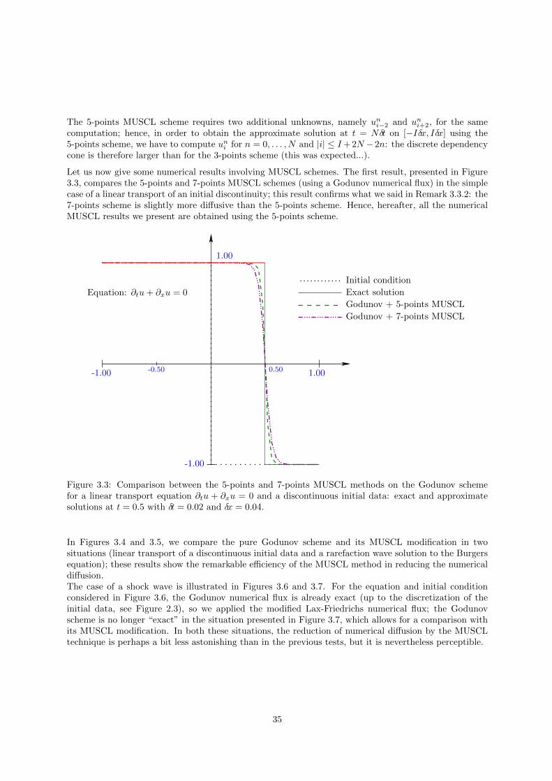
The 5-points MUSCL scheme requires two additional unknowns, namely uni−2 and uni+2, for the samecomputation; hence, in order to obtain the approximate solution at t = Nδt on [−Iδx, Iδx] using the5-points scheme, we have to compute uni for n = 0, . . . , N and |i| ≤ I+ 2N −2n: the discrete dependencycone is therefore larger than for the 3-points scheme (this was expected...).

Let us now give some numerical results involving MUSCL schemes. The first result, presented in Figure3.3, compares the 5-points and 7-points MUSCL schemes (using a Godunov numerical flux) in the simplecase of a linear transport of an initial discontinuity; this result confirms what we said in Remark 3.3.2: the7-points scheme is slightly more diffusive than the 5-points scheme. Hence, hereafter, all the numericalMUSCL results we present are obtained using the 5-points scheme.

Godunov + 5-points MUSCL

Godunov + 7-points MUSCL

Exact solution

Initial condition

-1.00 1.00-0.50

1.00

-1.00

0.50

Equation: ∂tu+ ∂xu = 0

Figure 3.3: Comparison between the 5-points and 7-points MUSCL methods on the Godunov schemefor a linear transport equation ∂tu + ∂xu = 0 and a discontinuous initial data: exact and approximatesolutions at t = 0.5 with δt = 0.02 and δx = 0.04.

In Figures 3.4 and 3.5, we compare the pure Godunov scheme and its MUSCL modification in twosituations (linear transport of a discontinuous initial data and a rarefaction wave solution to the Burgersequation); these results show the remarkable efficiency of the MUSCL method in reducing the numericaldiffusion.The case of a shock wave is illustrated in Figures 3.6 and 3.7. For the equation and initial conditionconsidered in Figure 3.6, the Godunov numerical flux is already exact (up to the discretization of theinitial data, see Figure 2.3), so we applied the modified Lax-Friedrichs numerical flux; the Godunovscheme is no longer “exact” in the situation presented in Figure 3.7, which allows for a comparison withits MUSCL modification. In both these situations, the reduction of numerical diffusion by the MUSCLtechnique is perhaps a bit less astonishing than in the previous tests, but it is nevertheless perceptible.

35

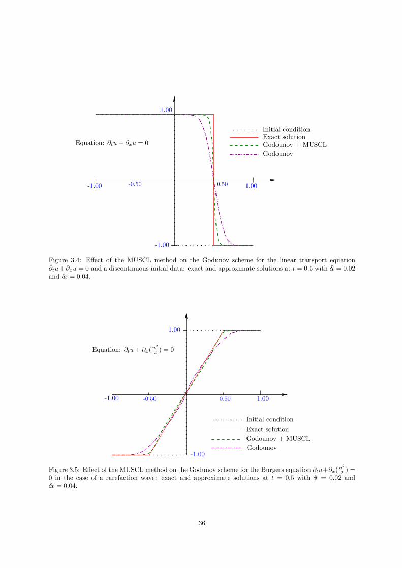
-1.00 1.00

1.00

-1.00

0.50-0.50

Equation: ∂tu+ ∂xu = 0

Godounov

Godounov + MUSCLExact solutionInitial condition

Figure 3.4: Effect of the MUSCL method on the Godunov scheme for the linear transport equation∂tu+∂xu = 0 and a discontinuous initial data: exact and approximate solutions at t = 0.5 with δt = 0.02and δx = 0.04.

-1.00

1.00

-1.00

-0.50 0.50

Godounov + MUSCL

Initial condition

Exact solution

Godounov

Equation: ∂tu+ ∂x(u2

2 ) = 0

1.00

Figure 3.5: Effect of the MUSCL method on the Godunov scheme for the Burgers equation ∂tu+∂x(u2

2 ) =0 in the case of a rarefaction wave: exact and approximate solutions at t = 0.5 with δt = 0.02 andδx = 0.04.

36

-1.00

-1.00 1.00

1.00

Initial condition and exact solution

Modified Lax-Friedrichs + MUSCL

Modified Lax-Friedrichs

Equation: ∂tu+ ∂x(u2

2 ) = 0

Figure 3.6: Effect of the MUSCL method on the modified Lax-Friedrichs scheme for the Burgers equation

∂tu + ∂x(u2

2 ) = 0 in the case of a shock: exact and approximate solutions at t = 0.5 with δt = 0.02 andδx = 0.04.

Godounov + MUSCL

Initial condition

Exact solution

Godounov

Equation: ∂tu+ ∂x(u2

2 ) = 0

-1.00 1.00-0.50 0.50

1.00

0.50

Figure 3.7: Effect of the MUSCL method on the Godunov scheme for the Burgers equation ∂tu+∂x(u2

2 ) =0 in the case of a shock: exact and approximate solutions at t = 0.5 with δt = 0.02 and δx = 0.04.

37

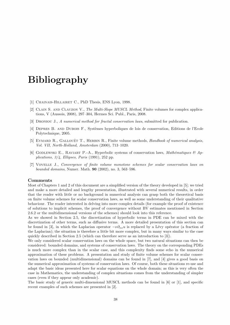
Bibliography

[1] Chainais-Hillairet C., PhD Thesis, ENS Lyon, 1998.

[2] Clain S. and Clauzon V., The Multi-Slope MUSCL Method, Finite volumes for complex applica-tions, V (Aussois, 2008), 297–304, Hermes Sci. Publ., Paris, 2008.

[3] Droniou J., A numerical method for fractal conservation laws, submitted for publication.

[4] Depres B. and Dubois F., Systemes hyperboliques de lois de conservation, Editions de l’EcolePolytechnique, 2005.

[5] Eymard R., Gallouet T., Herbin R., Finite volume methods, Handbook of numerical analysis,Vol. VII, North-Holland, Amsterdam (2000), 713–1020.

[6] Godlewski E., Raviart P.-A., Hyperbolic systems of conservation laws, Mathematiques & Ap-plications, 3/4, Ellipses, Paris (1991), 252 pp.

[7] Vovelle J., Convergence of finite volume monotone schemes for scalar conservation laws onbounded domains, Numer. Math. 90 (2002), no. 3, 563–596.

CommentsMost of Chapters 1 and 2 of this document are a simplified version of the theory developed in [5]; we triedand make a more detailed and lengthy presentation, illustrated with several numerical results, in orderthat the reader with little or no background in numerical analysis can grasp both the theoretical basison finite volume schemes for scalar conservation laws, as well as some understanding of their qualitativebehaviour. The reader interested in delving into more complex details (for example the proof of existenceof solutions to implicit schemes, the proof of convergence without BV estimates mentioned in Section2.6.2 or the multidimensional versions of the schemes) should look into this reference.As we showed in Section 2.5, the discretization of hyperbolic terms in PDE can be mixed with thediscretization of other terms, such as diffusive terms. A more detailed presentation of this section canbe found in [3], in which the Laplacian operator −ν∂xxu is replaced by a Levy operator (a fraction ofthe Laplacian); the situation is therefore a little bit more complex, but in many ways similar to the casequickly described in Section 2.5 (which can therefore serve as an introduction to [3]).We only considered scalar conservation laws on the whole space, but two natural situations can then beconsidered: bounded domains, and systems of conservation laws. The theory on the corresponding PDEsis much more complex than in the scalar case, and this complexity finds some echo in the numericalapproximation of these problems. A presentation and study of finite volume schemes for scalar conser-vation laws on bounded (multidimensional) domains can be found in [7], and [4] gives a good basis onthe numerical approximation of systems of conservation laws. Of course, both these situations re-use andadapt the basic ideas presented here for scalar equations on the whole domain; as this is very often thecase in Mathematics, the understanding of complex situations comes from the understanding of simplercases (even if they appear only academic).The basic study of generic multi-dimensional MUSCL methods can be found in [6] or [1], and specificrecent examples of such schemes are presented in [2].

38