A Beam Tracing Approach to Acoustic Modeling forInteractive Virtual Environments

Thomas Funkhouser�, Ingrid Carlbom, Gary Elko,

Gopal Pingali, Mohan Sondhi, and Jim WestBell Laboratories

Abstract

Virtual environment research has focused on interactive image gen-eration and has largely ignored acoustic modeling for spatializationof sound. Yet, realistic auditory cues can complement and enhancevisual cues to aid navigation, comprehension, and sense of presencein virtual environments. A primary challenge in acoustic model-ing is computation of reverberation paths from sound sources fastenough for real-time auralization. We have developed a system thatuses precomputed spatial subdivision and “beam tree” data struc-tures to enable real-time acoustic modeling and auralization in inter-active virtual environments. The spatial subdivision is a partition of3D space into convex polyhedral regions (cells) represented as a celladjacency graph. A beam tracing algorithm recursively traces pyra-midal beams through the spatial subdivision to construct a beam treedata structure representing the regions of space reachable by eachpotential sequence of transmission and specular reflection events atcell boundaries. From these precomputed data structures, we cangenerate high-order specular reflection and transmission paths atinteractive rates to spatialize fixed sound sources in real-time as theuser moves through a virtual environment. Unlike previous acousticmodeling work, our beam tracing method: 1) supports evaluation ofreverberation paths at interactive rates, 2) scales to compute high-order reflections and large environments, and 3) extends naturallyto compute paths of diffraction and diffuse reflection efficiently. Weare using this system to develop interactive applications in which auser experiences a virtual environment immersively via simultane-ous auralization and visualization.

Key Words: Beam tracing, acoustic modeling, auralization,spatialized sound, virtual environment systems, virtual reality.

1 Introduction

Interactive virtual environment systems combine graphics, acous-tics, and haptics to simulate the experience of immersive explorationof a three-dimensional virtual world by rendering the environmentas perceived from the viewpoint of an observer moving under real-time control by the user. Most prior research in virtual environmentsystems has focused on visualization (i.e., methods for renderingmore realistic images or for increasing image refresh rates), whilerelatively little attention has been paid to auralization (i.e., renderingspatialized sound based on acoustical modeling). Yet, it is clear that

�Princeton University

we must pay more attention to producing realistic sound in order tocreate a complete immersive experience in which aural cues com-bine with visual cues to support more natural interaction within avirtual environment. First, qualitative changes in sound reverbera-tion, such as more absorption in a room with more lush carpets, canenhance and reinforce visual comprehension of the environment.Second, spatialized sound can be useful for providing audio cuesto aid navigation, communication, and sense of presence [14]. Forexample, the sounds of objects requiring user attention can be spa-tialized according to their positions in order to aid object locationand binaural selectivity of desired signals (e.g., “cocktail party” ef-fect). The goal of this work is to augment a previous interactiveimage generation system to support real-time auralization of soundbased on realistic acoustic modeling in large virtual environments.We hope to use this system to support virtual environment appli-cations such as distributed training, simulation, education, homeshopping, virtual meetings, and multiplayer games.

A primary challenge in acoustic modeling is computation ofreverberation paths from a sound source to a listener (receiver) [30].As sound may travel from source to receiver via a multitude ofreflection, transmission, and diffraction paths, accurate simulationis extremely compute intensive. For instance, consider the simpleexample shown in Figure 1. In order to present an accurate modelof a sound source (labeled ‘S’) at a receiver location (labeled ‘R’),we must account for an infinite number of possible reverberationpaths (some of which are shown). If we are able to model thereverberation paths from a sound source to a receiver, we can rendera spatialized representation of the sound according to their delays,attenuations, and source and receiver directivities.

S R

Figure 1: Example reverberation paths.

Since sound and light are both wave phenomena, acoustic mod-eling is similar to global illumination in computer graphics. How-ever, there are several significant differences. First, the wavelengthsof audible sound fall between 0.02 and 17 meters (20kHz to 20Hz),more than five orders of magnitude longer than visible light. As aresult, though reflection of sound waves off large walls tends to beprimarily specular, significant diffraction does occur around edgesof objects like walls and tables. Small objects (like coffee mugs)have significant effect on the sound field only at frequencies beyond4 kHz, and can usually be excluded from models of acoustic en-vironments, especially in the presence of other significant sourcesof reflection and diffraction. Second, sound travels through air 106

times slower than light, causing significantly different arrival timesfor sound propagating along different paths, and the resulting acous-tic signal is perceived as a combination of direct and reflected sound

(reverberation). The time distribution of the reverberation pathsof the� sound in a typical room is much longer than the integrationperiod of the perception of sound by a human. Thus, it is importantto accurately compute the exact time/frequency distribution of thereverberation. In contrast, the speed of light and the perception oflight is such that the eye integrates out the transient response of alight source and only the energy steady-state response needs to becalculated. Third, since sound is a coherent wave phenomenon, thecalculation of the reflected and scattered sound waves must incor-porate the phase (complex amplitude) of the incident and reflectedwave(s), while for incoherent light, only the power must be summed.

Although acoustic modeling has been well-studied in the con-text of non-interactive applications [34], such as concert hall design,there has been relatively little prior research in real-time acousticmodeling for virtual environment systems [15]. Currently availableauralization systems generally model only early specular reflections,while late reverberations and diffractions are modeled with statisti-cal approximations [1, 25, 40, 53]. Also, due to the computationalcomplexity of current systems, they generally consider only simplegeometric arrangements and low-order specular reflections. For in-stance, the Acoustetron [17] computes only first- and second-orderspecular reflections for box-shaped virtual environments. Videogames provide spatialized sound with ad hoc localization methods(e.g., pan effects) rather than with realistic geometrical acousticmodeling methods. The 1995 National Research Council Report onVirtual Reality Scientific and Technological Challenges [15] statesthat “current technology is still unable to provide interactive systemswith real-time rendering of acoustic environments with complex, re-alistic room reflections.”

In this paper, we describe a beam tracing method that computeshigh-order specular reflection and transmission paths from fixedsources in large polygonal models fast enough to be used for au-ralization in interactive virtual environment systems. The key ideabehind our method is to precompute and store spatial data struc-tures that encode all possible transmission and specular reflectionpaths from each audio source and then use these data structures tocompute reverberation paths to an arbitrarily moving observer view-point for real-time auralization during an interactive user session.Our algorithms for construction and query of these data structureshave the unique features that they scale well with increasing num-bers of reflections and global geometric complexity, and they extendnaturally to model paths of diffraction and diffuse reflection. Wehave incorporated these algorithms and data structures into a systemthat supports real-time auralization and visualization of large virtualenvironments.

2 Previous Work

There has been a large amount of work in acoustic modeling. Priormethods can be classified into four types: 1) image source methods,2) radiant exchange methods 3) path tracing, and 4) beam tracing.

2.1 Image Source Methods

Image source methods [2, 6] compute specular reflection paths byconsidering virtual sources generated by mirroring the location ofthe audio source,

�, over each polygonal surface of the environment

(see Figure 2). For each virtual source,���

, a specular reflection pathcan be constructed by iterative intersection of a line segment fromthe source position to the receiver position, � , with the reflectingsurface planes (such a path is shown for virtual source

���in Fig-

ure 2). Specular reflection paths can be computed up to any orderby recursive generation of virtual sources.

The primary advantage of image source methods is their robust-ness. They can guarantee that all specular paths up to a given orderor reverberation time will be found. The disadvantages of imagesource methods are that they model only specular reflections, and

S

R

Sa Sb

Sc

Sd

a

b

cd

Figure 2: Image source method.

their expected computational complexity has exponential growth. Ingeneral, � ����� virtual sources must be generated for � reflectionsin environments with � surface planes. Moreover, in all but the sim-plest environments (e.g., a box), complex validity/visibility checksmust be performed for each of the � ����� virtual sources since notall of the virtual sources represent physically realizable specularreflection paths [6]. For instance, a virtual source generated byreflection over the non-reflective side of a surface is “invalid.” Like-wise, a virtual source whose reflection is blocked by another surfacein the environment or intersects a point on a surface’s plane whichis outside the surface’s boundary (e.g.,

���in Figure 2) is “invisi-

ble.” During recursive generation of virtual sources, descendentsof invalid virtual sources can be ignored. However, descendents ofinvisible virtual sources must still be considered, as higher-orderreflections may generate visible virtual sources (consider mirroring� �

over surface � ). Due to the computational demands of � ����� vis-ibility checks, image source methods are practical only for acousticmodeling of few reflections in simple environments [32].

2.2 Radiant Exchange Methods

Radiant exchange methods have been used extensively in computergraphics to model diffuse reflection of radiosity between patches[21]. Briefly, radiosity methods consider every patch a potentialemitter and reflector of radiosity. Conceptually, for every pair ofpatches, � and � , a form factor is computed which measures thefraction of the radiosity leaving patch � that arrives at patch � . Thisapproach yields a set of simultaneous equations which are solved toobtain the radiosity for each patch.

Although this approach has been used with good results formodeling diffuse indirect illumination in computer graphics, it isnot easily extensible to acoustics. In acoustics modeling, transportequations must account for phase, specular reflection tends to dom-inate diffuse reflection, and “extended form factor” computationsmust consider paths of diffraction as well as specular reflection. Fur-thermore, to meet error tolerances suitable for acoustic modeling,patches must be substructured to a very fine element mesh (typi-cally much less than the acoustic wavelength), the solution must becomputed for many frequencies, and the representation of the soundleaving an element must be very data intensive, a complex func-tion of phase, direction, and frequency usually requiring thousandsof bytes. As a result, direct extensions to prior radiosity methods[36, 39, 52] do not seem practical for large environments.

2.3 Path Tracing Methods

Ray tracing methods [33, 61] find reverberation paths between asource and receiver by generating rays emanating from the sourceposition and following them through the environment until an ap-propriate set of rays has been found that reach a representation ofthe receiver position (see Figure 3).

Monte Carlo path tracing methods consider randomly gener-ated paths from the source to the receiver [28]. For instance, theMetropolis Light Transport algorithm [54] generates a sequence oflight transport paths by randomly mutating a single current path by

SR

Figure 3: Ray tracing method.

adding, deleting, or replacing vertices. Mutated paths are acceptedaccording to probabilities based on the estimated contribution theymake to the solution. As contributing paths are found, they arelogged and then mutated further to generate new paths in a Markovchain. Mutation strategies and acceptance probabilities are chosento insure that the method is unbiased, stratified, and ergodic.

A primary advantage of these methods is their simplicity. Theydepend only on ray-surface intersection calculations, which are rel-atively easy to implement and have computational complexity thatgrows sublinearly with the number of surfaces in the model. Anotheradvantage is generality. As each ray-surface intersection is found,paths of specular reflection, diffuse reflection, diffraction, and re-fraction can be sampled [10], thereby modeling arbitrary types ofindirect reverberation, even for models with curved surfaces.

The primary disadvantages of path tracing methods stem fromthe fact that the continuous 5D space of rays is sampled by a dis-crete set of paths, leading to aliasing and errors in predicted roomresponses [35]. For instance, in ray tracing, the receiver positionand diffracting edges are often approximated by volumes of space(in order to admit intersections with infinitely thin rays), which canlead to false hits and paths counted multiple times [35]. Moreover,important reverberation paths may be missed by all samples. Inorder to minimize the likelihood of large errors, path tracing sys-tems often generate a large number of samples, which requires alarge amount of computation. Another disadvantage of path tracingis that the results are dependent on a particular receiver position,and thus these methods are not directly applicable in virtual envi-ronment applications where either the source or receiver is movingcontinuously.

2.4 Beam Tracing Methods

Beam tracing methods [23] classify reflection paths from a source byrecursively tracing pyramidal beams (i.e., sets of rays) through theenvironment. Briefly, a set of pyramidal beams are constructed thatcompletely cover the 2D space of directions from the source. Foreach beam, polygons are considered for intersection in order fromfront to back. As intersecting polygons are detected, the originalbeam is clipped to remove the shadow region, a transmission beamis constructed matching the shadow region, and a reflection beam isconstructed by mirroring the transmission beam over the polygon’splane (see Figure 4).

Original Beam

Reflection Beam

Transmission Beam

S’S

ab c

Figure 4: Beam tracing method.

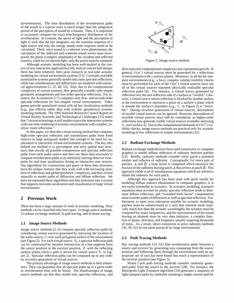
As compared to image source methods, the primary advantageof beam tracing is that fewer virtual sources must be considered forenvironments with arbitrary geometry. Since each beam representsthe region of space for which a corresponding virtual source (at theapex of the beam) is visible, higher-order virtual sources must be

considered only for reflections of polygons intersecting the beam.For instance, in Figure 5, consider the virtual source

���, which

results from reflection of�

over polygon � . The correspondingreflection beam, � � , contains exactly the set of receiver points forwhich

���is valid and visible. Similarly, � � intersects exactly the

set of polygons ( � and � ) for which second-order reflections arepossible after specular reflection off polygon � . Other polygons( � , � , � , and � ) need not be considered for second order specularreflections after � . Beam tracing allows the recursion tree of virtualsources to be pruned significantly. On the other hand, the imagesource method is more efficient for a box-shaped environment forwhich a regular lattice of virtual sources can be constructed that areguaranteed to be visible for all receiver locations [2].

Sa S

d

a

Rab

e

fg

c

Figure 5: Beam tracing culls invisible virtual sources.

As compared to path tracing methods, the primary advantageof beam tracing is that it takes advantage of spatial coherence, aseach beam-surface intersection represents an infinite number of ray-surface intersections. Also, pyramidal beam tracing does not sufferfrom sampling artifacts of ray tracing [35] or the overlap problems ofcone tracing [3, 55], since the entire 2D space of directions leavingthe source can be covered by beams exactly.

The primary disadvantage of beam tracing is that the geometricoperations required to trace a beam through a 3D model (i.e., inter-section and clipping) are relatively complex, as each beam may bereflected and/or obstructed by several surfaces. Another limitationis that reflections off curved surfaces and refractions are difficult tomodel.

Geometric beam tracing has been used in a variety of appli-cations, including acoustic modeling [13, 38, 46, 57], illumination[9, 19, 20, 22, 23, 59], and radio propagation [16]. The chal-lenge is to perform geometric operations (i.e., intersection, clipping,and mirroring) on beams efficiently as they are traced recursivelythrough a complex environment.

Some systems avoid the geometric complexity of beam tracingby approximating each beam by its medial axis ray for intersectionand mirror operations [36], possibly splitting rays as they divergewith distance [31, 42]. In this case, the beam representation is onlyuseful for modeling the distribution of rays/energy with distanceand for avoiding large tolerances in ray-receiver intersection calcu-lations. If beams are not clipped or split when they intersect morethan one surface, significant reverberation paths can be missed.

Heckbert and Hanrahan [23] described an algorithm for illumi-nation in which pyramidal beams represented by their 2D polygonalcross-sections are traced recursively either forward from a viewpointor backward from a point light source. For each beam, all polygonsare processed in front to back order. For each polygon intersectingthe beam, the shadow region is “cut out” of the original beam usinga polygon clipping algorithm capable of handling concavities andholes. The authors describe construction of an intermediate “lightbeam tree” data structure that encodes the beam tracing recursionand is used for later evaluation of light paths. Their implementationdoes not scale well to large environments since its computationalcomplexity grows with � � 2 � for � polygons.

Dadoun et al. [12, 13] described a beam tracing algorithmfor acoustic modeling in which a hierarchical scene representation(HSR) is used to accelerate polygon sorting and intersection testing.During a preprocessing phase, a binary space partition (BSP) tree

structure is constructed and augmented with storage for the convexhull for

�each subtree. Then, during beam tracing, the HSR is used to

accelerate queries to find an ordered set of polygons potentially in-tersecting each beam. As in [23], beams are represented by their 2Dpolygonal cross-sections and are updated using the Weiler-Athertonclipping algorithm [60] at polygon intersections.

Fortune [16] described a beam tracing algorithm for indoor radiopropagation prediction in which a spatial data structure comprising“layers” of 2D triangulations is used to accelerate polygon intersec-tion testing. A method is proposed in which beams are partitionedinto convex regions by planes supporting the edges of occludingpolygons. However, Fortune expects that method to be too expen-sive for use in indoor radio propagation (where attenuation due totransmission is small) due to the exponential growth in the numberof beams. Instead, he has implemented a system in which beamsare traced directly from the source and along paths of reflection, butare not clipped by occluding polygons. Instead, attenuation due toocclusion is computed for each path, taking into account the attenua-tion of each occluding polygon along the path. This implementationtrades-off more expensive computation during path generation forless expensive computation during beam tracing.

Jones [27] and Teller [51] have described beam tracing algo-rithms to compute a “potentially visible set” of polygons to renderfrom a particular viewpoint in a computer graphics scene. Thesealgorithms preprocess the scene into a spatial subdivision of cells(convex polyhedra) and portals (transparent, boundaries betweencells). Polyhedral beams are traced through portals to determinethe region of space potentially visible from a view frustum in orderto produce a conservative and approximate solution to the hiddensurface problem.

In this paper, we describe beam tracing data structures andalgorithms for real-time acoustic modeling in interactive virtualenvironment applications. Our method is most closely related towork in [23] and [51]. As compared to previous acoustic modelingmethods, the unique features of our method are the ability to: 1)generate specular reflection and transmission paths at interactiverates, 2) scale to support large virtual environments, 3) scale tocompute high-order reflection and transmission paths, and 4) extendto support efficient computation of diffraction and diffuse reflectionpaths. We have included these algorithms and data structures inan interactive virtual environment system that supports immersiveauralization and visualization in complex polygonal environments.

3 System Organization

Our virtual environment system takes as input: 1) a description of thegeometry and visual/acoustic surface properties of the environment(i.e., sets of polygons), and 2) a set of anechoic audio source signalsat fixed locations. As a user moves through the virtual environmentinteractively, the system generates images as seen from a simulatedobserver viewpoint, along with a stereo audio signal spatializedaccording to the computed reverberation paths from each audiosource to the observer location.

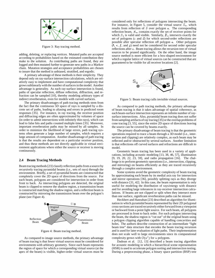
In order to support real-time auralization, we partition our sys-tem into four distinct phases (see Figure 6), two of which are pre-processing steps that execute off-line, while the last two executein real-time as a user interactively controls an observer viewpointmoving through a virtual environment. First, during the spatial sub-division phase, we precompute spatial relationships inherent in theset of polygons describing the environment and represent them in acell adjacency graph data structure that supports efficient traversalsof space. Second, during the beam tracing phase, we recursivelyfollow beams of transmission and specular reflection through spacefor each audio source. The output of the beam tracing phase is abeam tree data structure that explicitly encodes the region of spacereachable by each sequence of reflection and transmission pathsfrom each source point. Third, during the path generation phase,

we compute reverberation paths from each source to the receivervia lookup into the precomputed beam tree data structure as thereceiver (i.e., the observer viewpoint) is moved under interactiveuser control. Finally, during the auralization phase, we spatializeeach source audio signal (in stereo) according to the lengths, atten-uations, and directions of the computed reverberation paths. Thespatialized audio output is synchronized with real-time graphicsoutput to provide an immersive virtual environment experience.

Geometry,AcousticProperties

SpatialSubdivision

CellAdjacency Graph

BeamTracing

Beam Tree

PathGeneration

Reverberation Paths

ReceiverPosition and Direction

SourcePosition and Direction

Auralization

Spatialized Audio

Source Audio

Figure 6: System organization.

3.1 Spatial Subdivision

Our system preprocesses the geometric properties of the environ-ment and builds a spatial subdivision to accelerate beam tracing.The goal of this phase is to precompute spatial relationships in-herent in the set of polygons describing the environment and torepresent them in a data structure that supports efficient traversalsof space. The spatial subdivision is constructed by partitioning 3Dspace into a set of convex polyhedral regions and building a graphthat explicitly represents the adjacencies between the regions of thesubdivision.

We build the spatial subdivision using a Binary Space Partition(BSP) [18], a recursive binary split of 3D space into convex polyhe-dral regions (cells) separated by planes. To construct the BSP, werecursively split cells by candidate planes selected by the methoddescribed in [41]. The binary splitting process continues until noinput polygon intersects the interior of any BSP cell. The result ofthe BSP is a set of convex polyhedral cells whose convex, planarboundaries contain all the input polygons.

An adjacency graph is constructed that explicitly representsthe neighbor relationships between cells of the spatial subdivision.Each cell of the BSP is represented by a node in the graph, and twonodes have a link between them for each planar, polygonal boundaryshared by the corresponding adjacent cells in the spatial subdivision.Construction of the cell adjacency graph is integrated with the binaryspace partitioning algorithm. If a leaf in the BSP is split into two bya plane, we create new nodes in the graph corresponding to the newcells in the BSP, and we update the links of the split leaf’s neighborsto reflect the new adjacencies. We create a separate link betweentwo cells for each convex polygonal region that is entirely eithertransparent or opaque along the cells’ shared boundary.

A simple 2D example model (on left) and its cell adjacencygraph (on right) are shown in Figure 7. Input “polygons” appear assolid line segments labeled with lower-case letters ( ���! ); transpar-ent cell boundaries introduced by the BSP are shown as dashed linesegments labeled with lower-case letters ( �"�$# ); constructed cellregions are labeled with upper-case letters ( �%�'& ); and, links aredrawn between adjacent cells sharing a convex “polygonal” bound-ary.

b

q(

a d k

l

o

h

cf

e

g

i

j)

m n

p

(a) Input model.

A

B

CD

E

c

b

q*

a d k

l

o

h

f

e

g+i

m n

pEpC

j,r

tsu

(b) Cell adjacency graph.

Figure 7: Example spatial subdivision.

3.2 Beam Tracing

After the spatial subdivision has been constructed, we use it to accel-erate traversals of space in our beam tracing algorithm. Beams aretraced through the cell adjacency graph via a recursive depth-firsttraversal starting in the cell containing the source point. Adjacentcells are visited recursively while a beam representing the regionof space reachable from the source by a sequence of cell bound-ary reflection and transmission events is incrementally updated. Asthe algorithm traverses a cell boundary into a new cell, the currentconvex pyramidal beam is “clipped” to include only the region ofspace passing through the convex polygonal boundary polygon. Atreflecting cell boundaries, the beam is mirrored across the planesupporting the cell boundary in order to model specular reflections.As an example, Figure 8 shows a sequence of beams (green polyhe-dra) traced up to one reflection from a source (white point) throughthe spatial subdivision (blue ‘X’s are cell boundaries) for a simpleset of input polygons (red surfaces).

Figure 8: A beam clipped and reflected at cell boundaries.

Throughout the traversal, the algorithm maintains a current cell(a reference to a cell in the spatial subdivision) and a current beam(an infinite convex pyramidal beam whose apex is the source point).Initially, the current cell is set to be the cell containing the sourcepoint and the current beam is set to cover all of space. During eachstep of the depth-first traversal, the algorithm continues recursivelyfor each boundary polygon, - , of the current cell, . , that intersectsthe current beam, � . If - does not coincide with an opaque inputsurface, the algorithm follows a transmission path, recursing tothe cell adjacent to . across - with a transmission beam, �0/ ,constructed as the intersection of � with a pyramidal beam whoseapex is the source point and whose sides pass through the edgesof - . Likewise, if - coincides with a reflecting input surface,the algorithm follows a specular reflection path, recursing in cell. with a specular reflection beam, � � , constructed by mirroringthe transmission beam over the plane supporting - . The depth-firsttraversal along any path terminates when the length of a path exceedsa user-specified threshold or when the cumulative absorption due totransmission and reflection exceeds a preset threshold. The traversalmay also be terminated when the total number of reflections ortransmissions exceeds a third threshold.

Figure 9 contains an illustration of the beam tracing algorithmexecution for specular reflections through the simple 2D example

model shown in Figure 7. The depth-first traversal starts in thecell (labeled ‘D’) containing the source point (labeled ‘S’) with abeam containing the entire cell (shown as dark green). Beams arecreated and traced for each of the six boundary polygons of cell ‘D’(1 , 2 , 3 , 4 , � , and # ). For example, transmission through the cellboundary labeled ‘ # ’ results in a beam (labeled 5�6 ) that is trimmedas it enters cell ‘E.’ 5�6 intersects only the polygon labeled ‘ 7 ,’ whichspawnsa reflection beam (labeled 5�68�09 ). That beam intersects onlythe polygon labeled ‘: ,’ which spawns a reflection beam (labeled5�6;�<9=�?> ). Execution continues recursively for each beam until thelength of every path exceeds a user-specified threshold or when theabsorption along every path becomes too large.

A

B

CD

E

S

op@

us Tu

TuRoTuRoRpt

Figure 9: Beam tracing through cell adjacency graph.

While tracing beams through the spatial subdivision, our algo-rithm constructs a beam tree data structure [23] to be used for rapiddetermination of reverberation paths from the source point later dur-ing the path generation phase. The beam tree corresponds directly tothe recursion tree generated during the depth-first traversal throughthe cell adjacency graph. It is similar to the “stab tree” data struc-ture used by Teller to encode visibility relationships for occlusionculling [51]. Each node of the beam tree stores: 1) a reference to thecell being traversed, 2) the cell boundary most recently traversed(if there is one), and 3) the convex beam representing the regionof space reachable by the sequence of reflection and transmissionevents along the current path of the depth-first traversal. To furtheraccelerate reverberation path generation, each node of the beam treealso stores the cumulative attenuation due to reflective and trans-missive absorption, and each cell of the spatial subdivision stores alist of “back-pointers” to its beam tree nodes. Figure 10 shows apartial beam tree corresponding to the traversal shown in Figure 9.

D

EDD D DDk j m nu l

Eo

EpA

Ct

B C CCsi gB f

q c

B B

Figure 10: Beam tree.

3.3 Path Generation

During an interactive session in which the user navigates a simulatedobserver (receiver) through the virtual environment, reverberationpaths from a particular source point,

�, to the moving receiver

point, � , can be generated quickly via lookup in the beam tree datastructure. First, the cell containing the receiver point is found bylogarithmic-time search of the BSP. Then, each beam tree node,5 , associated with that cell is checked to see whether the beamstored with 5 contains the receiver point. If it does, a viable raypath from the source point to the receiver point has been found,and the ancestors of 5 in the beam tree explicitly encode the set ofreflections and transmissions through the boundaries of the spatialsubdivision that a ray must traverse from the source to the receiveralong this path (more generally, to any point inside the beam storedwith 5 ).

The attenuation, length, and directional vectors for the corre-sponding reverberation path can be derived quickly from the datastored with the beam tree node, 5 . Specifically, the attenuation dueto reflection and transmission can be retrieved from 5 directly. Thelength of the reverberation path and the directional vectors at thesource and receiver points can be easily computed as the source’sreflected image for this path is stored explicitly in 5 as the apexof its pyramidal beam. The actual ray path from the source pointto the receiver point can be generated by iterative intersection withthe reflecting cell boundaries stored with the ancestors of 5 . Forexample, Figure 11 shows the specular reflection path to a particularreceiver point (labeled ‘R’) for the example shown in Figure 9.

A

B

CD

E

S

pC

u

tsR

Ip

Ioo

So

Sop

Figure 11: Reverberation path to receiver point (‘R’) computed vialookup in beam tree for source point (‘S’).

3.4 Auralization

Once a set of reverberation paths from a source to the receiver hasbeen computed, the source-receiver impulse response is generatedby adding one pulse corresponding to each distinct path from thesource to the receiver. The delay associated with each pulse is givenby D�EF. , where D is the length of the corresponding reverberationpath, and . is the speed of sound. Since the pulse is attenuatedby every reflection and dispersion, the amplitude of each pulseis given by �GEHD , where � is the product of all the frequency-independent reflectivity and transmission coefficients for each ofthe reflecting and transmitting surfaces along the correspondingreverberation path.

At the receiver, the binaural impulse responses (response ofthe left and right ears) are different due to the directivity of eachear. These binaural impulse responses are generated by multiply-ing each pulse of the impulse response by the cardioid directivityfunction (1 E 2 1 I cos KJL��� , where J is the angle of arrival of thepulse with respect to the normal vector pointing out of the ear) cor-responding to each ear. This rough approximation to actual headscattering and diffraction is similar to the standard two-point stereomicrophone technique used in high fidelity audio recording. Fi-nally, the (anechoic) input audio signal is auralized by convolving it

with the binaural impulse responses to produce a stereo spatializedaudio signal. In the future, we intend to incorporate source direc-tivity, frequency-dependent absorption [34], and angle-dependentabsorption [11, 43] into our acoustic models.

A separate, concurrently executing process is spawned to per-form convolution of the computed binaural impulse responses withthe input audio signal. In order to support real-time auralization,transfer of the impulse responses from the path generation processto the convolution process utilizes double buffers synchronized bya semaphore. Each new pair of impulse responses is loaded by thepath generation process into a “back buffer” as the convolution pro-cess continues to access the current impulse responses stored in the“front buffer.” A semaphore is used to synchronize the processes asthe front and back buffer are switched.

4 Results

The 3D data structures and algorithms described in the precedingsections have been implemented in C++ and run on Silicon Graphicsand PC/Windows computers.

To test whether the algorithms scale well as the complexity of the3D environment and the number of specular reflections increase, weexecuted a series of experiments with our system computing spatialsubdivisions, beam trees, and specular reflection paths for variousarchitectural models of different complexities. Our test modelsranged from a simple box to a complex building, Soda Hall, thecomputer science building at UC Berkeley (an image and descriptionof each test model appears in Figure 12). The experiments were runon a Silicon Graphics Octane workstation with 640MB of memoryand used one 195MHz R10000 processor.

(a) Box: 1 cube.(6 polygons)

(c) Suite: 9 rooms in office space.(184 polygons)

(e) Floor: M 50 rooms of Soda Hall.(1,772 polygons)

(b) Rooms: 2 rooms connected by door.(20 polygons)

(d) Maze: 16 rooms connected by hallways.(602 polygons)

(f) Building: M 250 rooms of Soda Hall.(10,057 polygons)

Figure 12: Test models (source locations are gray dots).

4.1 Spatial Subdivision Results

We first constructed the spatial subdivision data structure (cell ad-jacency graph) for each test model. Statistics from this phase ofthe experiment are shown in Table 1. Column 2 lists the numberof input polygons in each model, while Columns 3 and 4 contain

the numbers of cells and links, respectively, generated by the spatialsubdiN vision algorithm. Column 5 contains the wall-clock time (inseconds) for the algorithm to execute, while Column 6 shows thestorage requirements (in MBs) for the resulting spatial subdivision.

Model # # # Time StorageName Polys Cells Links (sec) (MB)

Box 6 7 18 0.0 0.004Rooms 20 12 43 0.1 0.029Suite 184 98 581 3.0 0.352Maze 602 172 1,187 4.9 0.803Floor 1,772 814 5,533 22.7 3.310Bldg 10,057 4,512 31,681 186.3 18.694

Table 1: Spatial subdivision statistics.

Empirically, we find that the numbers of cells and links createdby our spatial subdivision algorithm grow linearly with the numberof input polygons for typical architectural models (see Figure 13),rather than quadratically as is possible for worst case geometric ar-rangements. The reason for linear growth can be seen intuitivelyin the two images inlaid in Figure 13, which compare spatial sub-divisions for the Maze test model (on the left) and a 2x2 grid ofMaze test models (on the right). The 2x2 grid of Mazes has ex-actly four times as many polygons and approximately four times asmany cells. The storage requirements of the spatial subdivision datastructure also grow linearly as they are dominated by the vertices oflink polygons.

0 11K1K 2K 6K3K 4K 5K 7K 8K 9K 10K

# C

ells

in S

patia

l Sub

divi

sion

# Polygons in Environment

5K

4K

3K

2K

1K

Maze

2x2 Grid of Mazes

Figure 13: Plot of subdivision size vs. polygonal complexity.

The time required to construct the spatial subdivisions growssuper-linearly, dominated by the code that selects and orders split-ting planes during BSP construction (see [41]). It is important tonote that the spatial subdivision phase must be executed only onceoff-line for each geometric model, as its results are stored in a file,allowing rapid reconstruction in subsequent beam tracing execu-tions.

4.2 Beam Tracing Results

We experimented with our beam tracing algorithm for sixteen sourcelocations in each test model. The source locations were chosen torepresent typical audio source positions (e.g., in offices, in commonareas, etc.) – they are shown as gray dots in Figure 12 (experimentswith the Building test used the same source locations as are shownin the Floor model). For each source location, we traced beams (i.e.,constructed a beam tree) five times, each time with a different limiton the maximum number of specular reflections (e.g., up to 0, 1, 2,4, or 8 reflections). Other termination criteria based on attenuationor path length were disabled, and transmission was ignored, in order

to isolate the impact of input model size and maximum number ofspecular reflections on computational complexity.

Table 2 contains statistics gathered during the beam tracingexperiment – each row represents an execution with a particular testmodel and maximum number of reflections, averaged over all 16source locations. Columns 2 and 3 show the number of polygonsdescribing each test model and the maximum number of specularreflections allowed in each test, respectively. Column 4 contains theaverage number of beams traced by our algorithm (i.e., the averagenumber of nodes in the resulting beam trees), and Column 5 showsthe average wall-clock time (in milliseconds) for the beam tracingalgorithm to execute.

Beam Tracing Path GenerationModel # # # Time # TimeName Polys Rfl Beams (ms) Paths (ms)

Box 6 0 1 0 1.0 0.01 7 1 7.0 0.12 37 3 25.0 0.34 473 42 129.0 6.08 10,036 825 833.0 228.2

Rooms 20 0 3 0 1.0 0.01 31 3 7.0 0.12 177 16 25.1 0.34 1,939 178 127.9 5.28 33,877 3,024 794.4 180.3

Suite 184 0 7 1 1.0 0.01 90 9 6.8 0.12 576 59 25.3 0.44 7,217 722 120.2 6.58 132,920 13,070 672.5 188.9

Maze 602 0 11 1 0.4 0.01 167 16 2.3 0.02 1,162 107 8.6 0.14 13,874 1,272 36.2 2.08 236,891 21,519 183.1 46.7

Floor 1,772 0 23 4 1.0 0.01 289 39 6.1 0.12 1,713 213 21.5 0.44 18,239 2,097 93.7 5.38 294,635 32,061 467.0 124.5

Bldg 10,057 0 28 5 1.0 0.01 347 49 6.3 0.12 2,135 293 22.7 0.44 23,264 2,830 101.8 6.88 411,640 48,650 529.8 169.5

Table 2: Beam tracing and path generation statistics.

Scale with Increasing Polygonal Complexity

We readily see from the results in Column 4 that the number of beamstraced by our algorithm (i.e., the number of nodes in the beam tree)does not grow at an exponential rate with the number of polygonsin these environments (as it does using the image source method).Each beam traced by our algorithm pre-classifies the regions ofspace according to whether the corresponding virtual source (i.e.,the apex of the beam) is visible to a receiver. Rather than generating� ��� virtual sources (beams) at each step of the recursion as in theimage source method, we directly find only the potentially visiblevirtual sources via beam-polygon intersection and cell adjacencygraph traversal. We use the current beam and the current cell of thespatial subdivision to find the small set of polygon reflections thatadmit visible higher-order virtual sources.

The benefit of this approach is particularly important for largeenvironments in which the boundary of each convex cell is sim-ple, and yet the entire environment is very complex. As an ex-ample, consider computation of up to 8 specular reflections in theBuilding test model (the last row of Table 2). The image sourcemethod must consider approximately 1,851,082,741 virtual sources( O 8

��P 0 10 Q 057 E 2 � � ), assuming half of the 10,057 polygons arefront-facing to each virtual source. Our beam tracing method con-

siders only 411,640 virtual sources, a difference of four orders ofmagnitude.R In most cases, it would be impractical to build and storethe recursion tree without such effective pruning.

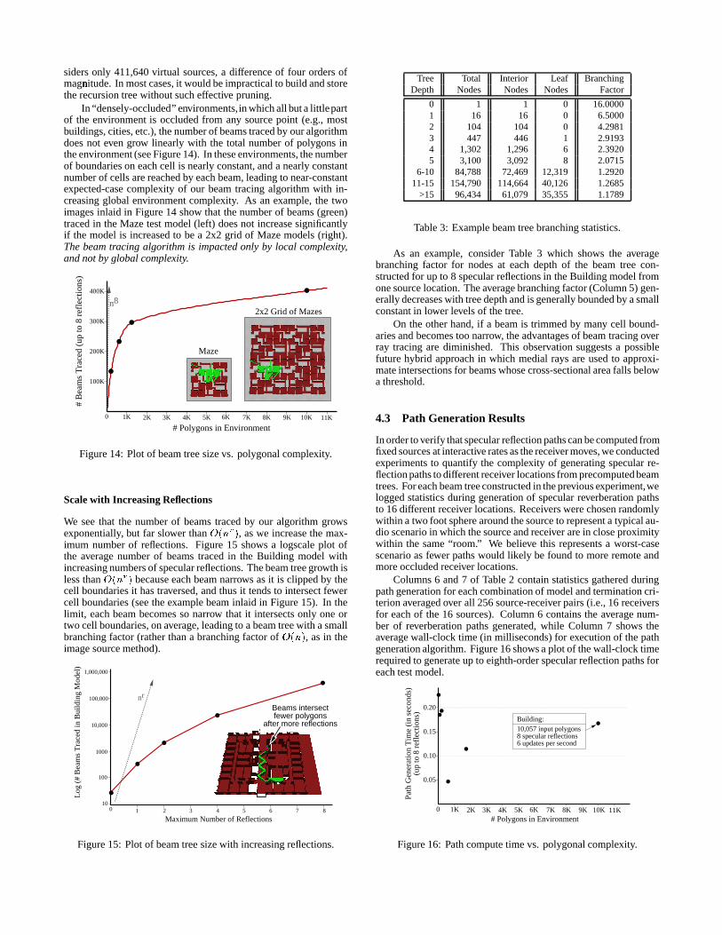
In “densely-occluded” environments,in which all but a littlepartof the environment is occluded from any source point (e.g., mostbuildings, cities, etc.), the number of beams traced by our algorithmdoes not even grow linearly with the total number of polygons inthe environment (see Figure 14). In these environments, the numberof boundaries on each cell is nearly constant, and a nearly constantnumber of cells are reached by each beam, leading to near-constantexpected-case complexity of our beam tracing algorithm with in-creasing global environment complexity. As an example, the twoimages inlaid in Figure 14 show that the number of beams (green)traced in the Maze test model (left) does not increase significantlyif the model is increased to be a 2x2 grid of Maze models (right).The beam tracing algorithm is impacted only by local complexity,and not by global complexity.

0 11K1K 2K 6K3K 4K 5K 7K 8K 9K 10K

100K

200K

300K

400K

# B

eam

s T

race

d (u

p to

8 r

efle

ctio

ns)

# Polygons in Environment

Maze

2x2 Grid of Mazesn8

Figure 14: Plot of beam tree size vs. polygonal complexity.

Scale with Increasing Reflections

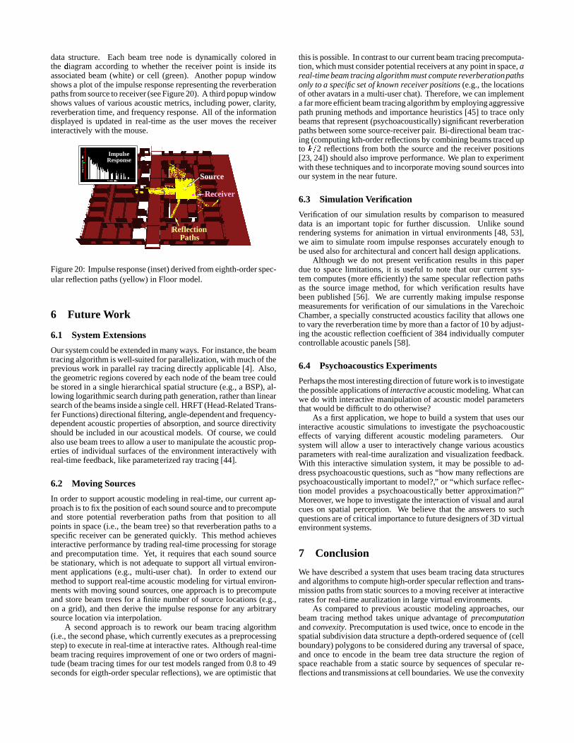
We see that the number of beams traced by our algorithm growsexponentially, but far slower than � � � � , as we increase the max-imum number of reflections. Figure 15 shows a logscale plot ofthe average number of beams traced in the Building model withincreasing numbers of specular reflections. The beam tree growth isless than � � � � because each beam narrows as it is clipped by thecell boundaries it has traversed, and thus it tends to intersect fewercell boundaries (see the example beam inlaid in Figure 15). In thelimit, each beam becomes so narrow that it intersects only one ortwo cell boundaries, on average, leading to a beam tree with a smallbranching factor (rather than a branching factor of � ��� , as in theimage source method).

0

Log

(#

Bea

ms

Tra

ced

in B

uild

ing

Mod

el)

Maximum Number of Reflections1 2 3 4 5 6 7 8

10

100

1000

10,000

100,000

1,000,000

nr

Beams intersect fewer polygons

after more reflections

Figure 15: Plot of beam tree size with increasing reflections.

Tree Total Interior Leaf BranchingDepth Nodes Nodes Nodes Factor

0 1 1 0 16.00001 16 16 0 6.50002 104 104 0 4.29813 447 446 1 2.91934 1,302 1,296 6 2.39205 3,100 3,092 8 2.0715

6-10 84,788 72,469 12,319 1.292011-15 154,790 114,664 40,126 1.2685

>15 96,434 61,079 35,355 1.1789

Table 3: Example beam tree branching statistics.

As an example, consider Table 3 which shows the averagebranching factor for nodes at each depth of the beam tree con-structed for up to 8 specular reflections in the Building model fromone source location. The average branching factor (Column 5) gen-erally decreases with tree depth and is generally bounded by a smallconstant in lower levels of the tree.

On the other hand, if a beam is trimmed by many cell bound-aries and becomes too narrow, the advantages of beam tracing overray tracing are diminished. This observation suggests a possiblefuture hybrid approach in which medial rays are used to approxi-mate intersections for beams whose cross-sectional area falls belowa threshold.

4.3 Path Generation Results

In order to verify that specular reflection paths can be computed fromfixed sources at interactive rates as the receiver moves, we conductedexperiments to quantify the complexity of generating specular re-flection paths to different receiver locations from precomputed beamtrees. For each beam tree constructed in the previous experiment,welogged statistics during generation of specular reverberation pathsto 16 different receiver locations. Receivers were chosen randomlywithin a two foot sphere around the source to represent a typical au-dio scenario in which the source and receiver are in close proximitywithin the same “room.” We believe this represents a worst-casescenario as fewer paths would likely be found to more remote andmore occluded receiver locations.

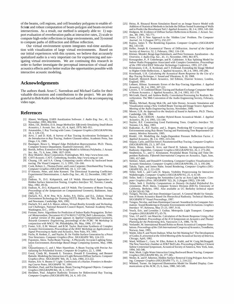
Columns 6 and 7 of Table 2 contain statistics gathered duringpath generation for each combination of model and termination cri-terion averaged over all 256 source-receiver pairs (i.e., 16 receiversfor each of the 16 sources). Column 6 contains the average num-ber of reverberation paths generated, while Column 7 shows theaverage wall-clock time (in milliseconds) for execution of the pathgeneration algorithm. Figure 16 shows a plot of the wall-clock timerequired to generate up to eighth-order specular reflection paths foreach test model.

0 11K1K 2K 6K3K 4K 5K 7K 8K 9K 10K

0.05

0.10

0.15

0.20

Path

Gen

erat

ion

Tim

e (i

n se

cond

s)(u

p to

8 r

efle

ctio

ns)

# Polygons in Environment

Building:10,057 input polygons8 specular reflections6 updates per second

Figure 16: Path compute time vs. polygonal complexity.

We find that the number of specular reflection paths betweena sourceS and receiver in close proximity of one another is nearlyconstant across all of our test models. Also, the time required byour path generation algorithm is generally not dependent on thenumber of polygons in the environment (see Figure 16), nor is itdependent on the total number of nodes in the precomputed beamtree. This result is due to the fact that our path generation algorithmconsiders only nodes of the beam tree with beams residing insidethe cell containing the receiver location. Therefore, the computationtime required by the algorithm is not dependent on the complexityof the whole environment, but instead on the number of beams thattraverse the receiver’s cell.

Overall, we find that our algorithm supports generation of spec-ular reflection paths between a fixed source and any (arbitrarilymoving) receiver at interactive rates in complex environments. Forinstance, we are able to compute up to 8th order specular reflectionpaths in the Building environment with more than 10,000 polygonsat a rate of approximately 6 times per second (i.e., the rightmostpoint in the plot of Figure 16).

4.4 Auralization Results

We have integrated the acoustic modeling method described in thispaper into an interactive system for audio/visual exploration of vir-tual environments (e.g., using VRML). The system allows a user tomove through a virtual environment while images and spatializedaudio are rendered in real-time according to the user’s simulatedviewpoint. Figure 17 shows one application we have developed,called VirtualWorks, in which a user may interact with objects (e.g.,click on them with the mouse) in the virtual environment to invokebehaviors that present information in various media, including text,image, video, and spatialized audio. For instance, if the user clickson the workstation sitting on the desk, the application invokes avideo which is displayed on the screen of that workstation. Weare using this system to experiment with 3D user interfaces forpresentation of multimedia data and multi-user interaction.

We ran experiments with this application using a Silicon Graph-ics Octane workstation with 640MB of memory and two 195MHzR10000 processors. One processor was used for image generationand acoustic modeling (i.e., reverberation path generation), whilethe second processor was dedicated solely to auralization (i.e., con-volution of the computed stereo impulse responses with audio sig-nals).

Due to the differences between graphics and acoustics describedin Section 1, the geometry and surface characteristics of the virtualenvironment were input and represented in two separate forms,one for graphics and another for acoustics. The graphical model(shown in Figure 17) was represented as a scene graph containing80,372 polygons, most of which describe the furniture and othersmall, detailed, visually-important objects in the environment. Theacoustical model contained only 184 polygons, which describedthe ceilings, walls, cubicles, floors, and other large, acoustically-important features of the environment (it was identical to the Suitetest model shown in Figure 12c).

We gathered statistics during sample executions of this ap-plication. Figures 17b-c show an observer viewpoint path (red)along which the application was able to render between eight andtwelve images per second, while simultaneously auralizing four au-dio sources (labeled 1-4) in stereo according to fourth-order specularreflection paths updated during each frame. While walking alongthis path, it was possible to notice subtle acoustic effects due toreflections and occlusions. In particular, near the viewpoint labeled‘A’ in Figure 17b, audio source ‘2’ became very reverberant due toreflections (cyan lines) in the long room. Likewise, audio source ‘3’suddenly became much louder and then softer as the observer passedby an open doorway near the viewpoint labeled ‘B’ in Figure 17c.

Throughout our experiments, the auralization process was thebottleneck. Our C++ convolution code running on a R10000 pro-

cessor could execute fast enough to output 8 KHz stereo audio for aset of impulse responses cumulatively containing around 500 non-zero elements. We are planning to integrate DSP-based hardware[37] with our system to implement real-time convolution in the nearfuture.

5 Discussion

5.1 Geometric Limitations

Our method is not practical for all virtual environments. First, thegeometric input must comprise only planar polygons. Each acousticreflector is assumed to be locally reacting and to have dimensionsfar exceeding the wavelength of audible sound (since initially weare assuming that specular reflections are the dominant componentsof reverberation).

Second, the efficiency of our method is greatly impacted bythe complexity and quality of the constructed spatial subdivision.For best results, the polygons should be connected (e.g., withoutsmall cracks between them) and arranged such that a large part ofthe model is occluded from any position in space (e.g., like mostbuildings or cities). Specifically,our method would not perform wellfor geometric models with high local geometric complexity (e.g.,a forest of trees). In these cases, beams traced through boundariesof cells enclosing free space would quickly become fragmentedinto many smaller beams, leading to disadvantageous growth of thebeam tree. For this reason, our method is not as well suited forglobal illumination as it is for acoustic modeling, in which smallobjects can be ignored and large surfaces can be modeled with littlegeometric surface detail due to the longer wavelengths of audiblesound.

Third, the major occluding and reflecting surfaces of the virtualenvironment must be static during interactive path generation andauralization. If any acoustically significant polygon moves, thespatial subdivision and every beam tree must be recomputed.

The class of geometric models for which our method does workwell includes most architectural and urban environments. In thesemodels, acoustically significant surfaces are generally planar, large,and stationary, and the acoustical effects of any sound source arelimited to a local region of the environment.

5.2 Diffraction and Diffuse Reflection

Our current 3D implementation traces beams only along paths ofspecular reflection and transmission, and it does not model otherscattering effects. Of course, paths of diffraction and diffuse re-flection are also important for accurate acoustic modeling [34, 26].Fortunately, our beam tracing algorithm and beam tree represen-tation can be generalized to model these effects. For instance,new beams can be traced that enclose the region of space reachedby diffracting and diffuse reflection paths, and new nodes can beadded to the beam tree representing diffractions and diffuse reflec-tion events at cell boundaries. For these more complex scatteringphenomena, the geometry of the beams is most useful for comput-ing candidate reverberation paths, while the amplitude of the signalalong any of the these paths can be evaluated for a known receiverduring path generation. We have already included these extensionsin a 2D beam tracing implementation, and we are currently workingon a similar 3D implementation.

First, consider diffraction. According to the Geometrical The-ory of Diffraction [29], an acoustic field that is incident on a dis-continuity along an edge has a diffracted wave that propagates intothe shadow region. The diffracted wave can be modeled in geo-metric terms by considering the edge to be a source of new wavesemanating from the edge. Higher order reflections and diffractionsoccur as diffracted waves impinge upon other surfaces and edgediscontinuities. By using edge-based adjacency information in our

(a)

13

2

4

A

(b)

13

2

4

B

(c)

Figure 17: VirtualWorks application. User’s view is shown in (a), while a bird’s eye view of fourth-order reverberation paths (color codedlines) from four sources (numbered circles) to Viewpoints ‘A’ and ‘B’ (black circles) are shown in (b) and (c), respectively.

spatial subdivision data structure, we can quickly perform the geo-metric operations required to construct and trace beams along pathsof diffraction. For a given beam, we can find edges causing diffrac-tion, as they are the ones: 1) intersected by the beam, and 2) sharedby cell boundaries with different acoustic properties (e.g., one istransparent and another is opaque). For each such edge, we candetermine the region of space reached by diffraction at that edgeby tracing a beam whose “source” coincides with the portion ofthe edge intersected by the impinging beam, and whose extent isbounded by the solid wedge of opaque surfaces sharing the edge.For densely-occluded environments, each such diffraction beam canbe computed and traced in expected-case constant time.

Second, consider diffuse reflection. We may model complexreflections and diffractions from some highly faceted surfaces asdiffuse reflections from planar surfaces emanating equally in alldirections. To compute the region of space reached by such a reflec-tion using our approach, we can construct a beam whose “source”is the convex polygonal region of the surface intersected by an im-pinging beam and whose initial extent encloses the entire halfspacein front of the surface. We can trace the beam through the celladjacency graph to find the region of space reached from any pointon the reflecting part of the surface (i.e., the anti-penumbra [50]).

We have implemented these methods so far in 2D using a pla-nar winged-edge representation [5] for the spatial subdivision anda bow-tie representation [49] for the beams. Unfortunately, tracing3D “beams” of diffraction and diffuse reflection is more compli-cated. First, the source of each diffraction beam is no longer apoint, but a finite edge, and the source of each diffuse reflectionbeam is generally a convex polygon. Second, as we trace suchbeams through the spatial subdivision, splitting and trimming themas they passes through multiple convex polygonal cell boundaries,their bounding surfaces can become quadric surfaces (i.e., reguli)[50]. Finally, evaluation of the amplitude of the signal along a“path” of diffraction or diffuse reflection requires integration over(possibly multiple) edges and polygons. We are currently extendingour 3D data structures and algorithms to model these effects. Ini-tially, we are planning to trace polyhedral beams that conservativelyover-estimate the region covered by an exact, more complex, repre-sentation of the scattering patterns. Then, as each reverberation pathto a particular receiver is considered, we will check whether it lieswithin the exact scattering region, or whether it should be discardedbecause it lies in the over-estimating region of the polyhedral beam.

5.3 Visualization

In order to aid understanding and debugging of our acoustic model-ing method, we have found it extremely valuable to use interactivevisualization. So far, we have concentrated on visualization of ourdata structures and algorithms. Our system provides menu and key-board commands that may be used to toggle display of the: 1) inputpolygons (red), 2) source point (white), 3) receiver point (purple),4) boundaries of the spatial subdivision (gray), 5) pyramidal beams

(green), 6) image sources (cyan), and 7) reverberation paths (yel-low). The system also supports visualization of acoustic metrics(e.g., power, clarity, etc.) computed for a set of receiver locationson a regular planar grid displayed with a textured polygon. Examplevisualizations are shown in Figures 18-20.

S

Beams

PowerLevels(Gray)

SR

Reflection Paths

Figure 18: Eighth-order specular reflection beams (left) and pre-dicted power levels (right) in Maze model.

Of course, many commercial [7, 8, 40] and research systems[38, 47] provide elaborate tools for visualizing computed acousticmetrics. The critical difference in our system is that it supportscontinuous interactive updates of reverberation paths and debugginginformation as a user moves the receiver point with the mouse. Forinstance, Figures 18 and 20 show eighth-order specular reflectionpaths (yellow lines) from a single audio source (white points) to areceiver location (purple points) which can be updated more thansix times per second as the receiver location is moved arbitrarily.The user may select any reverberation path for further inspectionby clicking on it and then independently toggle display of reflectingcell boundaries, transmitting cell boundaries, and the associated setof pyramidal beams for the selected path.

Source

Receiver

Beams

Figure 19: Beams (green) containing all eighth-order specular re-flection paths from a source to a receiver in City model.

Separate pop-up windows provide real-time display of otheruseful visual debugging and acoustic modeling information. Forinstance, one popup window shows a diagram of the beam tree

data structure. Each beam tree node is dynamically colored inthe diagramT according to whether the receiver point is inside itsassociated beam (white) or cell (green). Another popup windowshows a plot of the impulse response representing the reverberationpaths from source to receiver (see Figure 20). A third popup windowshows values of various acoustic metrics, including power, clarity,reverberation time, and frequency response. All of the informationdisplayed is updated in real-time as the user moves the receiverinteractively with the mouse.

time

amplitude

Source

Receiver

Reflection Paths

ImpulseResponse

Figure 20: Impulse response (inset) derived from eighth-order spec-ular reflection paths (yellow) in Floor model.

6 Future Work

6.1 System Extensions

Our system could be extended in many ways. For instance, the beamtracing algorithm is well-suited for parallelization, with much of theprevious work in parallel ray tracing directly applicable [4]. Also,the geometric regions covered by each node of the beam tree couldbe stored in a single hierarchical spatial structure (e.g., a BSP), al-lowing logarithmic search during path generation, rather than linearsearch of the beams inside a single cell. HRFT (Head-Related Trans-fer Functions) directional filtering, angle-dependent and frequency-dependent acoustic properties of absorption, and source directivityshould be included in our acoustical models. Of course, we couldalso use beam trees to allow a user to manipulate the acoustic prop-erties of individual surfaces of the environment interactively withreal-time feedback, like parameterized ray tracing [44].

6.2 Moving Sources

In order to support acoustic modeling in real-time, our current ap-proach is to fix the position of each sound source and to precomputeand store potential reverberation paths from that position to allpoints in space (i.e., the beam tree) so that reverberation paths to aspecific receiver can be generated quickly. This method achievesinteractive performance by trading real-time processing for storageand precomputation time. Yet, it requires that each sound sourcebe stationary, which is not adequate to support all virtual environ-ment applications (e.g., multi-user chat). In order to extend ourmethod to support real-time acoustic modeling for virtual environ-ments with moving sound sources, one approach is to precomputeand store beam trees for a finite number of source locations (e.g.,on a grid), and then derive the impulse response for any arbitrarysource location via interpolation.

A second approach is to rework our beam tracing algorithm(i.e., the second phase, which currently executes as a preprocessingstep) to execute in real-time at interactive rates. Although real-timebeam tracing requires improvement of one or two orders of magni-tude (beam tracing times for our test models ranged from 0.8 to 49seconds for eigth-order specular reflections), we are optimistic that

this is possible. In contrast to our current beam tracing precomputa-tion, which must consider potential receivers at any point in space, areal-time beam tracing algorithm must compute reverberationpathsonly to a specific set of known receiver positions (e.g., the locationsof other avatars in a multi-user chat). Therefore, we can implementa far more efficient beam tracing algorithm by employing aggressivepath pruning methods and importance heuristics [45] to trace onlybeams that represent (psychoacoustically) significant reverberationpaths between some source-receiver pair. Bi-directional beam trac-ing (computing kth-order reflections by combining beams traced upto 2UE 2 reflections from both the source and the receiver positions[23, 24]) should also improve performance. We plan to experimentwith these techniques and to incorporate moving sound sources intoour system in the near future.

6.3 Simulation Verification

Verification of our simulation results by comparison to measureddata is an important topic for further discussion. Unlike soundrendering systems for animation in virtual environments [48, 53],we aim to simulate room impulse responses accurately enough tobe used also for architectural and concert hall design applications.

Although we do not present verification results in this paperdue to space limitations, it is useful to note that our current sys-tem computes (more efficiently) the same specular reflection pathsas the source image method, for which verification results havebeen published [56]. We are currently making impulse responsemeasurements for verification of our simulations in the VarechoicChamber, a specially constructed acoustics facility that allows oneto vary the reverberation time by more than a factor of 10 by adjust-ing the acoustic reflection coefficient of 384 individually computercontrollable acoustic panels [58].

6.4 Psychoacoustics Experiments

Perhaps the most interesting direction of future work is to investigatethe possible applications of interactive acoustic modeling. What canwe do with interactive manipulation of acoustic model parametersthat would be difficult to do otherwise?

As a first application, we hope to build a system that uses ourinteractive acoustic simulations to investigate the psychoacousticeffects of varying different acoustic modeling parameters. Oursystem will allow a user to interactively change various acousticsparameters with real-time auralization and visualization feedback.With this interactive simulation system, it may be possible to ad-dress psychoacoustic questions, such as “how many reflections arepsychoacoustically important to model?,” or “which surface reflec-tion model provides a psychoacoustically better approximation?"Moreover, we hope to investigate the interaction of visual and auralcues on spatial perception. We believe that the answers to suchquestions are of critical importance to future designers of 3D virtualenvironment systems.

7 Conclusion

We have described a system that uses beam tracing data structuresand algorithms to compute high-order specular reflection and trans-mission paths from static sources to a moving receiver at interactiverates for real-time auralization in large virtual environments.

As compared to previous acoustic modeling approaches, ourbeam tracing method takes unique advantage of precomputationand convexity. Precomputation is used twice, once to encode in thespatial subdivision data structure a depth-ordered sequence of (cellboundary) polygons to be considered during any traversal of space,and once to encode in the beam tree data structure the region ofspace reachable from a static source by sequences of specular re-flections and transmissions at cell boundaries. We use the convexity

of the beams, cell regions, and cell boundary polygons to enable ef-ficientR and robust computation of beam-polygon and beam-receiverintersections. As a result, our method is uniquely able to: 1) sup-port evaluation of reverberation paths at interactive rates, 2) scale tocompute high-order reflections in large environments, and 3) extendto compute paths of diffraction and diffuse reflection.

Our virtual environment system integrates real-time auraliza-tion with visualization of large virtual environments. Based onour initial experiences with this system, we believe that accuratelyspatialized audio is a very important cue for experiencing and nav-igating virtual environments. We are continuing this research inorder to further investigate the perceptual interaction of visual andacoustics effects and to better realize the opportunities possible withinteractive acoustic modeling.

Acknowledgements

The authors thank Arun C. Surendran and Michael Gatlin for theirvaluable discussions and contributions to the project. We are alsograteful to Bob Kubli who helped record audio for the accompanyingvideo tape.

References[1] Ahnert, Wolfgang. EARS Auralization Software. J. Audio Eng. Soc., 41, 11,

November, 1993, 894-904.[2] Allen, J.B., Berkley, D.A. Image Method for Efficiently Simulating Small-Room

Acoustics, J. Acoust. Soc. Am., 65, 4, April, 1979, 943–951.[3] Amanatides, J. Ray Tracing with Cones. Computer Graphics (SIGGRAPH 84).

18, 3, 129-135.[4] Arvo, J. and D. Kirk. A Survey of Ray Tracing Acceleration Techniques. in

An Introduction to Ray Tracing, Andrew Glassner editor, Academic Press, SanDiego, CA, 1989.

[5] Baumgart, Bruce G. Winged Edge Polyhedron Representation. Ph.D. Thesis,Computer Science Department, Stanford University, 1972.

[6] Borish, Jeffrey. Extension of the Image Model to Arbitrary Polyhedra. J. Acoust.Soc. Am., 75, 6, June, 1984, 1827-1836.

[7] Bose Modeler, Bose Corporation, Framingham, MA. http://www.bose.com.[8] CATT-Acoustic, CATT, Gothenburg, Sweden, http://www.netg.se/ catt.[9] Chuang, J.H. and S.A. Cheng. Computing caustic effects by backward beam

tracing. The Visual Computer, 11, 3, 1995, 156–166.[10] Cook, Robert, L., Thomas Porter, and Loren Carpenter. Distributed Ray Tracing.

Computer Graphics (SIGGRAPH 84). 18, 3, 137-146.[11] D’Antonio, Peter, and John Konnert. The Directional Scattering Coefficient:

Experimental Determination. J, Audio Eng. Soc., 40, 12, December, 1992, 997-1017.

[12] Dadoun, N., D.G. Kirkpatrick, and J.P. Walsh. Hierarchical Approaches toHidden Surface Intersection Testing. Graphics Interface ‘82, Toronto, Canada,May, 1982, 49-56.

[13] Dadoun, N., D.G. Kirkpatrick, and J.P. Walsh. The Geometry of Beam Tracing.Proceedings of the Symposium on Computational Geometry, Baltimore, June,1985, 55-71.

[14] Durlach, N.I., R.W. Pew, W.A. Aviles, P.A. DiZio, and D.L. Zeltzer. VirtualEnvironment Technology for Training (VETT). Report No. 7661, Bolt, Beranek,and Newmann, Cambridge, MA, 1992.

[15] Durlach, N.I, and A.S. Mavor, editors, Virtual Reality Scientific and Technolog-ical Challenges, National Research Council Report, National Academy Press,Washington, D.C., 1995.

[16] Fortune, Steve. Algorithms for Prediction of Indoor Radio Propagation. Techni-cal Memorandum, Document #11274-960117-03TM, Bell Laboratories, 1996.A partial version of this paper appears in Applied Computational Geometry,Towards Geometric Engineering, proceedings of the FCRC ‘96 Workshop inconjunction with WACG ‘96, Philadelphia, PA, May, 1996, 157-166.

[17] Foster, S.H., E.M. Wenzel, and R.M. Taylor. Real-time Synthesis of ComplexAcoustic Environments. Proceedings of the IEEE Workshop on Applications ofSignal Processing to Audio and Acoustics, New Paltz, NY, 1991.

[18] Fuchs, H. Kedem, Z., and Naylor, B. On Visible Surface Generation by a PrioriTree Structures. Computer Graphics (Proc. SIGGRAPH ’80), 124-133.

[19] Fujomoto, Akira. Turbo Beam Tracing - A Physically Accurate Lighting Simu-lation Environment. Knowledge Based Image Computing Systems, May, 1988,1-5.

[20] Ghazanfarpour, G. and J. Marc Hasenfratz. A Beam Tracing with Precise An-tialiasing for Polyhedral Scenes. Computer & Graphics, 22, 1, 1998.

[21] Goral, Cindy M., Kenneth E. Torrance, Donald P. Greenberg, and BennettBattaile. Modeling the Interaction of Light Between Diffuse Surfaces. ComputerGraphics (Proc. SIGGRAPH ’84), 18, 3, July, 1984, 213-222.

[22] Haines, Eric A. Beams O’ Light: Confessions of a Hacker. Frontiers in Render-ing Course Notes, SIGGRAPH ’91, 1991.

[23] Heckbert, Paul, and Pat Hanrahan. Beam Tracing Polygonal Objects. ComputerGraphics (SIGGRAPH 84), 18, 3, 119-127.

[24] Heckbert, Paul. Adaptive Radiosity Textures for Bidirectional Ray Tracing.Computer Graphics (SIGGRAPH 90), 24, 4, 145-154.

[25] Heinz, R. Binaural Room Simulation Based on an Image Source Model withAddition of Statistical Methods to Include the Diffuse Sound Scattering of Wallsand to Predict the Reverberant Tail J. Applied Acoustics, 38, 2-4, 1993, 145-160.

[26] Hodgson, M. Evidence of Diffuse Surface Reflections in Rooms. J. Acoust. Soc.Am., 89, 1991, 765-771.

[27] Jones, C.B. A New Approach to the ‘Hidden Line’ Problem. The ComputerJournal, 14, 3 (August 1971), 232-237.

[28] Kajiya, James T. The Rendering Equation. Computer Graphics (SIGGRAPH86), 143-150.

[29] Keller, Joseph B. Geometrical Theory of Diffraction. Journal of the OpticalSociety of America, 52, 2, February, 1962, 116-130.

[30] Kleiner, Mendel, Bengt-Inge Dalenback, and Peter Svensson. Auralization – AnOverview. J. Audio Eng. Soc., 41, 11, November, 1993, 861-875.

[31] Kreuzgruber, P., P. Unterberger, and R. Gahleitner. A Ray Splitting Model forIndoor Radio Propagation Associated with Complex Geometries. Proceedingsof the 1993 43rd IEEE Vehicular Technology Conference, 1993, 227-230.

[32] Kristiansen, U.R., A. Krokstad, and T. Follestad. Extending the Image Methodto Higher-Order Reflections. J. Applied Acoustics, 38, 2-4, 1993, 195-206.

[33] Krockstadt, U.R. Calculating the Acoustical Room Response by the Use of aRay Tracing Technique, J. Sound and Vibrations, 8, 18, 1968.

[34] Kuttruff, Heinrich Room Acoustics, 3rd Edition, Elsevier Science, London,England, 1991.

[35] Lehnert, Hilmar. Systematic Errors of the Ray-Tracing Algorithm. J. AppliedAcoustics, 38, 2-4, 1993, 207-221.

[36] Lewers, T. A Combined Beam Tracing and Radiant Exchange Computer Modelof Room Acoustics. J. Applied Acoustics, 38, 2-4, 1993, 161-178.

[37] McGrath, David, and Andrew Reilly. Convolution Processing for Realistic Re-verberation. The 98th Convention of the Audio Engineering Society, February,1995.

[38] Monks, Michael, Byong Mok Oh, and Julie Dorsey. Acoustic Simulation andVisualization using a New Unified Beam Tracing and Image Source Approach.Meeting of the Audio Engineering Society, November, 1996.

[39] Moore, G.R. An Approach to the Analysis of Sound in Auditoria. Ph.D. Thesis,Cambridge, UK, 1984.

[40] Naylor, G.M. ODEON - Another Hybrid Room Acoustical Model. J. AppliedAcoustics, 38, 2-4, 1993, 131-144.

[41] Naylor, B.F. Constructing Good Partitioning Trees. Graphics Interface ‘93,Toronto, CA, May, 1993.

[42] Rajkumar, A., B.F. Naylor, and L. Rogers. Predicting RF Coverage in LargeEnvironments using Ray-Beam Tracing and Partitioning Tree Represented Ge-ometry. Wireless Networks, 1995.

[43] Rindel, J.H. Modelling the Angle-Dependent Pressure Reflection Factor. J.Applied Acoustics, 38, 2-4, 1993, 223-234.

[44] Sequin, Carlo, and Eliot Smyrl. Parameterized Ray Tracing. Computer Graphics(SIGGRAPH 89), 23, 3, 307-314.

[45] Smits, Brian, James R. Arvo, and David H. Salesin. An Importance-DrivenRadiosity Algorithm. Computer Graphics (SIGGRAPH 92), 26, 2, 273-282.

[46] Stephenson, U., and U. Kristiansen. Pyramidal Beam Tracing and Time De-pendent Radiosity. Fifteenth International Congress on Acoustics, Tapir, June,1995, 657-660.

[47] Stettner, Adam, and Donald P. Greenberg. Computer Graphics Visualization forAcoustic Simulation. Computer Graphics (SIGGRAPH 89), 23, 3, 195-206.

[48] Takala, Tapio, and James Hahn. Sound Rendering. Computer Graphics (SIG-GRAPH 92), 26, 2, 211-220.

[49] Teller, Seth J., and Carlo H. Sequin, Visibility Preprocessing for InteractiveWalkthroughs. Computer Graphics (SIGGRAPH 91), 25, 4, 61-69.

[50] Teller, Seth J. Computing the Antiumbra Cast by an Area Light Source. Com-puter Graphics (Proc. SIGGRAPH ’92), 26, 2 (August 1992), 139-148.

[51] Teller, Seth J. Visibility Computations in Densely Occluded Polyhedral En-vironments. Ph.D. thesis, Computer Science Division (EECS), University ofCalifornia, Berkeley, 1992. Also available as UC Berkeley technical reportUCB/CSD-92-708.

[52] Tsingos, Nicolas, and Jean-Dominique Gascuel. A General Model for Simula-tion of Room Acoustics Based On Hierarchical Radiosity. Technical Sketches,SIGGRAPH 97 Visual Proceedings, 1997.

[53] Tsingos, Nicolas, and Jean-Dominique Gascuel. Soundtracks for Computer Ani-mation: Sound Rendering in Dynamic Environments with Occlusions. GraphicsInterface ‘97, Kelowna, May 21-23, 1997, 9-16.

[54] Veach, Eric, and Leonidas J. Guibas. Metropolis Light Transport. ComputerGraphics (SIGGRAPH 97), 65-76.

[55] Vian, J.P. and D. van Maercke. Calculation of the Room Response Using a RayTracing Method. Proceedings of the ICA Symposium on Acoustics and TheaterPlanning for the Performing Arts, Vancouver, CA, 1986, 74-78.

[56] Vorlander, M. International Round Robin on Room Acoustical Computer Simu-lations. Proceedings of the 15th International Congressof Acoustics,Trondheim,Norway, June, 1995.

[57] Walsh, John P., and Norm Dadoun. What Are We Waiting for? The Developmentof Godot, II. presented at the 103rd Meeting of the Acoustical Society of America,Chicago, April, 1982.

[58] Ward, William C., Gary, W. Elko, Robert A. Kubli, and W. Craig McDougald.The New Varechoic chamber at AT&T BellLabs. Proceeding of Wallace ClementSabine Centennial Symposium, Acoustical Society of America, New York, June,1994, 343-346.

[59] Watt, Mark. Light-Water Interaction Using Backward Beam Tracing. ComputerGraphics (SIGGRAPH 90), 24, 377-385.

[60] Weiler, K. and P. Atherton. Hidden Surface Removal Using Polygon Area Sort-ing. Computer Graphics (SIGGRAPH 77), 11, 2, 214-222.

[61] Whitted, Turner. An Improved Illumination Model for Shaded Display. Com-munications of the ACM, 23, 6, June, 1980, 343-349.