Biometrics 70, 419–429 DOI: 10.1111/biom.12156June 2014

A Bayesian Localized Conditional Autoregressive Model forEstimating the Health Effects of Air Pollution

Duncan Lee,1,* Alastair Rushworth,1 and Sujit K. Sahu2

1School of Mathematics and Statistics, University of Glasgow, Glasgow G12 8QW, U.K.2Southampton Statistical Sciences Research Institute, University of Southampton,

Southampton SO17 1BJ, U.K.∗email: Duncan.Lee@glasgow.ac.uk

Summary. Estimation of the long-term health effects of air pollution is a challenging task, especially when modeling spatialsmall-area disease incidence data in an ecological study design. The challenge comes from the unobserved underlying spatialautocorrelation structure in these data, which is accounted for using random effects modeled by a globally smooth conditionalautoregressive model. These smooth random effects confound the effects of air pollution, which are also globally smooth. Toavoid this collinearity a Bayesian localized conditional autoregressive model is developed for the random effects. This localizedmodel is flexible spatially, in the sense that it is not only able to model areas of spatial smoothness, but also it is able to capturestep changes in the random effects surface. This methodological development allows us to improve the estimation performanceof the covariate effects, compared to using traditional conditional auto-regressive models. These results are established usinga simulation study, and are then illustrated with our motivating study on air pollution and respiratory ill health in GreaterGlasgow, Scotland in 2011. The model shows substantial health effects of particulate matter air pollution and nitrogen dioxide,whose effects have been consistently attenuated by the currently available globally smooth models.

Key words: Air pollution and health; Conditional autoregressive models; Spatial autocorrelation.

1. IntroductionQuantification of the health effects of air pollution is an im-portant problem of considerable public interest, both in termsof its financial and health impact. In the UK, the Departmentfor the Environment, Food and Rural Affairs (DEFRA) esti-mate that “in 2008 air pollution in the form of anthropogenicparticulate matter (PM) alone was estimated to reduce aver-age life expectancy in the UK by 6 months. Thereby imposingan estimated equivalent health cost of £19 billion” (DEFRAAir Quality Subject Group, 2010). These estimates are basedon large numbers of epidemiological studies, which have quan-tified the impact of both short-term and long-term expo-sure. The effects of long-term exposure can be estimated fromindividual-level cohort studies such as Laden et al. (2006) andBeverland et al. (2012), but they are expensive and time con-suming. Therefore ecological small-area study designs havealso been used, including Elliott et al. (2007), Lee, Ferguson,and Mitchell (2009), Haining et al. (2010), and Greven, Do-minici, and Zeger (2011). While these studies cannot assessthe causal health effects of air pollution due to their eco-logical design, they are quick and cheap to implement, andthey contribute to, and independently corroborate, the bodyof evidence about the long-term population level impact ofair pollution.

This ecological design is a form of geographical associa-tion study, where the study region is partitioned into non-overlapping areal units, such as counties or census tracts. Thenumber of disease cases observed in each areal unit is modeled,using Poisson regression, by risk factors including air pollution

concentrations, socio-economic deprivation, and demography.However, residual spatial autocorrelation may remain in thesedata, due to unmeasured confounding, neighborhood effects(where individual areal unit’s behavior is influenced by thatof neighboring units) and grouping effects (where individualunits seem to be close to similar units). This autocorrelation isaccounted for by adding a set of random effects to the model,which are usually represented by a conditional autoregressive(CAR; Besag, York, and Mollie, 1991) prior as part of a hier-archical Bayesian model.

The majority of CAR priors are globally smooth, and haverecently been shown by Reich, Hodges, and Zadnik (2006),Hodges and Reich (2010), Paciorek (2010), and Hughes andHaran (2013) to be potentially collinear with any covari-ate such as air pollution that is also globally smooth. Suchcollinearity leads to poor estimation performance for the fixedeffects, and additionally suggests that the residual spatial au-tocorrelation is unlikely to be globally spatially smooth asthat component of the spatial variation in the disease datawill have been accounted for. Instead, the residual spatialautocorrelation is likely to be strong in some areas showingsmoothness, and weak in some other areas exhibiting abruptstep changes. The widely used intrinsic and convolution CARmodels proposed by Besag et al. (1991) force the random ef-fects to exhibit a single global level of spatial smoothness de-termined by geographical adjacency, and are thus not flexibleenough to capture the complex localized structure likely tobe present in the residual spatial autocorrelation. The lack offlexibility in the intrinsic and convolution CAR models and

© 2014, The Authors Biometrics published by Wiley Periodicals, Inc. on behalf of International Biometric SocietyThis is an open access article under the terms of the Creative Commons Attribution License, which permits use,distribution and reproduction in any medium, provided the original work is properly cited.

419

420 Biometrics, June 2014

the collinearity problems highlighted by Hodges and Reich(2010) and others has motivated us to develop a new localizedconditional autoregressive (LCAR) prior for modeling residualspatial autocorrelation, which is presented in Section 3. Exist-ing solutions to these problems have been proposed by Reichet al. (2006), Hughes and Haran (2013), and Lee and Mitchell(2013), and a selection of them are compared by simulationto the LCAR prior proposed in this article in Section 4.

To contain the required flexibility, the LCAR prior captureslocalized residual spatial autocorrelation by allowing randomeffects in geographically adjacent areas to be autocorrelatedor conditionally independent, and we show that this priordistribution can have realizations at both spatial smoothingextremes, namely global smoothness and independence. How-ever, this flexibility leads to a large increase in the compu-tational burden and a lack of parsimony causing problems ofparameter identifiability, and a critique of the limitations ofthe existing literature in this area is given in Section 2. Here,we solve these problems with a novel prior elicitation methodbased on historical data, which is similar in spirit to powerpriors (see Chen and Ibrahim, 2006). Our elicitation is basedon an approximate Gaussian likelihood, and produces a setof candidate correlation structures for the residual spatial au-tocorrelation. The LCAR prior combines a discrete uniformdistribution on this set of candidate structures with a modi-fied CAR prior for the random effects, which combined withthe Poisson likelihood completes a full Bayesian hierarchicalmodel. Inference is obtained using Markov chain Monte Carlo(MCMC) methods, and the model allows us to simultaneouslyestimate the random effects, their local spatial structure aswell as the fixed effects. We conduct a large simulation studyin Section 4 to show improved parameter estimation when us-ing the proposed LCAR prior distribution. We follow up thisinvestigation by analyzing the motivating data set for the cityof Glasgow in Section 5. But first, we present the motivatingdata set and discuss the background modeling and prior dis-tributions in Section 2.

2. Background

2.1. Motivating Study

The study region is the health board comprising the city ofGlasgow and the river Clyde estuary, which in 2011 con-tained just under 1.2 million people. The region is parti-tioned into n = 271 administrative units called IntermediateGeographies (IG), which contain just over 4000 people on av-erage. The data used in this study are freely available, andcan be downloaded from the Scottish Neighbourhood Statis-tics (SNS) database (http://www.sns.gov.uk). The responsevariable is the numbers of admissions to non-psychiatric andnon-obstetric hospitals in each IG in 2011 with a primarydiagnosis of respiratory disease, which corresponds to codesJ00-J99 and R09.1 of the International Classification of Dis-ease tenth revision. Differences in the size and demographicstructure of the populations living in each IG are accountedfor by computing the expected numbers of hospital admissionsusing external standardization, based on age- and sex-specificrespiratory disease rates for the whole study region. An ex-ploratory estimate of disease risk is given by the standardizedincidence ratio (SIR), which is the ratio of the observed to

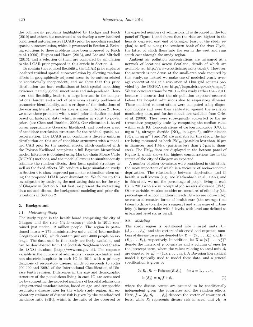
the expected numbers of admissions. It is displayed in the toppanel of Figure 1, and shows that the risks are highest in theheavily deprived east end of Glasgow (east of the study re-gion) as well as along the southern bank of the river Clyde,the latter of which flows into the sea in the west and runssouth east through the study region.

Ambient air pollution concentrations are measured at anetwork of locations across Scotland, details of which areavailable at http://www.scottishairquality.co.uk/. However,the network is not dense at the small-area scale required bythis study, so instead we make use of modeled yearly aver-age concentrations at a resolution of 1 km grid squares pro-vided by the DEFRA (see http://laqm.defra.gov.uk/maps/).We use concentrations for 2010 in this study rather than 2011,because it ensures that the air pollution exposure occurredbefore the hospital admissions due to respiratory illnesses.These modeled concentrations were computed using disper-sion models and were then calibrated against the availablemonitoring data, and further details are available from Griceet al. (2009). They were subsequently converted to the in-termediate geography scale by computing the median valuewithin each IG. Concentrations of carbon monoxide (CO, inmg m−3), nitrogen dioxide (NO2, in �g m−3), sulfur dioxide(SO2, in �g m−3) and PM are available for this study, the lat-ter being measured as both PM10 (particles less than 10 �min diameter) and PM2.5 (particles less than 2.5 �m in diam-eter). The PM10 data are displayed in the bottom panel ofFigure 1, which shows the highest concentrations are in thecenter of the city of Glasgow as expected.

A number of other covariates were considered in this study,the most important of which is a measure of socio-economicdeprivation. The relationship between deprivation and illhealth is well known (e.g., see Mackenbach et al., 1997), andin this study we use the percentage of people living in eachIG in 2010 who are in receipt of job seekers allowance (JSA).Other variables we also consider are measures of ethnicity (thepercentage of school children in each IG who are non-white),access to alternative forms of health care (the average timetaken to drive to a doctor’s surgery) and a measure of urban-icity (a factor variable with 6 levels, with level one defined asurban and level six as rural).

2.2. Modeling

The study region is partitioned into n areal units A ={A1, . . . ,An}, and the vectors of observed and expected num-bers of disease cases are denoted by Y = (Y1, . . . , Yn) and E =(E1, . . . , En), respectively. In addition, let X = (xT

1 , . . . ,xTn )T

denote the matrix of p covariates and a column of ones forthe intercept term, where the values relating to areal unit Ak

are denoted by xTk = (1, xk1, . . . , xkp). A Bayesian hierarchical

model is typically used to model these data, and a generalspecification is given by

Yk|Ek, Rk ∼ Poisson(EkRk) for k = 1, . . . , n,

ln(Rk) = xTk β + φk, (1)

where the disease counts are assumed to be conditionallyindependent given the covariates and the random effects.Here, β = (β0, β1, . . . , βp) denotes the vector of covariate ef-fects, while Rk represents disease risk in areal unit Ak. A

A Bayesian Localized Conditional Autoregressive Model 421

Easting

Nor

thin

g

650000

660000

670000

680000

220000 230000 240000 250000 260000 270000

0 5000 m0.6

0.8

1.0

1.2

1.4

1.6

1.8

2.0

Easting

Nor

thin

g

650000

660000

670000

680000

220000 230000 240000 250000 260000 270000

0 5000 m

10

11

12

13

14

15

16

17

18

Figure 1. Maps displaying the spatial pattern in the standardized incidence ratio for respiratory disease in 2011 (top panel)and the modeled yearly average concentration (in �g m−3) of PM10 in 2010 (bottom panel).

422 Biometrics, June 2014

value of Rk greater (less) than one indicates that areal unitAk has a higher (lower) than average disease risk, and interms of interpretation, Rk = 1.15 corresponds to a 15% in-creased risk of disease. As previously discussed, the ran-dom effects φ = (φ1, . . . , φn) capture any residual spatial au-tocorrelation present in the disease data, and are typicallyassigned a CAR prior, which is a special case of a Gaus-sian Markov random field (GMRF). Such models are typi-cally specified as a set of n univariate full conditional distri-butions, that is as f (φk|φ−k) for k = 1, . . . , n, where φ−k =(φ1, . . . , φk−1, φk+1, . . . , φn). However, the Markov nature ofthese models means that the conditioning is only on therandom effects in geographically adjacent areal units, whichinduces spatial autocorrelation into φ. The adjacency infor-mation comes from a binary n × n neighborhood matrix W,where wki equals one if areal units (Ak,Ai) share a commonborder (denoted k∼i) and is zero otherwise (denoted k � i).The intrinsic model (Besag et al., 1991; IAR) is the simplestprior in the CAR class, and its full conditional distributionsare given by

φk|φ−k, τ2,W ∼ N

(∑n

i=1wkiφi∑n

i=1wki

,τ2∑n

i=1wki

). (2)

The conditional expectation is the mean of the random ef-fects in neighboring areas, while the conditional variance isinversely proportional to the number of neighbors. The jointmultivariate Gaussian distribution for φ corresponding to (2)has a mean of zero but a singular precision matrix Q(W)/τ2,where Q(W) = diag(W1) − W, and 1 is an n dimensionalvector of ones. This prior is appropriate if the residuals fromthe covariate component of the model, that is ln(Y/E) − Xβ,are spatially smooth across the entire region, because the par-tial autocorrelation between (φk, φj) conditional on the re-maining random effects (denoted φ−kj) is

Corr[φk, φj|φ−kj,W] = wkj√(∑n

i=1wki)(

∑n

i=1wji)

. (3)

Equation (3) shows that all pairs of random effects relatingto geographically adjacent areal units are partially autocor-related (wkj = 1), which smoothes the random effects acrossgeographical borders. The most common extension to the IARmodel to allow for varying levels of spatial smoothness is theBYM or convolution model (Besag et al., 1991), which aug-ments the linear predictor in (1) with a second set of inde-pendent Gaussian random effects with a mean of zero anda constant variance. A further alternative using a single setof random effects was proposed by Stern and Cressie (1999),but this and other extensions have a single spatial autocor-relation parameter (for the BYM model it is the ratio of thetwo random effects variances) that controls the level of spa-tial smoothing globally across the entire region. Thus, thesemodels are inappropriate for capturing the likely localized na-ture of the residual spatial autocorrelation, which may containsub-region of spatial smoothness separated by step changes.

A small number of papers have extended the class of CARpriors to account for localized spatial smoothing, the majority

of which have treated W = {wkj|k∼j, k > j} as a set of binaryrandom quantities, rather than forcing them to equal one. Theneighborhood matrix is always assumed to be symmetric sothat changing wkj also changes wjk, while the other elementsin W relating to non-neighboring areal units remain fixed atzero. Equation (3) shows that this allows (φk, φj) correspond-ing to adjacent areal units to be conditionally independentor autocorrelated, and if wkj (and hence wjk) is estimated aszero a boundary is said to exist between the two random ef-fects. One of the first models in this vein was developed by Luet al. (2007), who proposed a logistic regression model for theelements in W, where the covariate was a non-negative mea-sure of the dissimilarity between areal units (Ak,Aj). Similarapproaches were proposed by Ma and Carlin (2007) and Ma,Carlin, and Banerjee (2010), who replace logistic regressionwith a second stage CAR prior and an Ising model, respec-tively. However, these approaches introduce a large numberof partial autocorrelation parameters into the model, whichfor the Glasgow data considered here has n = 271 data pointsand |W| = 718 partial autocorrelation parameters. Therefore,full estimation of W as a set of separate unknown parametersresults in a highly overparameterized precision matrix for φ,and Li, Banerjee, and McBean (2011) suggest that the indi-vidual elements are poorly identified from the data and arecomputationally expensive to update.

A related approach was proposed by Lee and Mitchell(2012), who deterministically model the elements of W as afunction of measures of dissimilarity and a small number ofparameters, rather than modeling each element as a separaterandom variable. However, their approach is designed for therelated fields of disease mapping and Wombling, whose aimsare not, as they are here, to estimate the effects of an expo-sure on a response. An alternative approach was suggestedby Lee and Mitchell (2013), who propose an iterative algo-rithm in which W is updated deterministically based on thejoint posterior distribution of the remaining model parame-ters. However, their algorithm has the drawback that onlyan estimate of each wkj is provided, rather than the poste-rior probability that wkj = 1. Finally, Reich et al. (2006) andHughes and Haran (2013) take an alternative approach, andforce the random effects to be orthogonal to the covariatesusing a residual projection matrix.

3. Methodology

Our methodological approach follows the majority of the lit-erature critiqued above, and treats the elements in W relatingto contiguous areal units as a set of binary random quantities.As CAR priors are a special case of an undirected graphicalmodel, we follow the terminology in that literature and referto W as the set of edges, and further define any edge wkj ∈ Wthat is estimated as zero as being removed. Our methodolog-ical innovation is a LCAR prior, which comprises a joint dis-tribution for an extended set of random effects φ and the setof edges W, rather than the traditional approach of assumingthe latter is fixed. We decompose this joint prior distributionas f (φ,W) = f (φ|W)f (W), and the next three sub-sectionsdescribe its two components as well as the overall hierarchicalmodel.

A Bayesian Localized Conditional Autoregressive Model 423

3.1. Prior Distribution - f (φ|W)

The IAR prior given by (2) is an inappropriate model forφ in the context of treating W as random, because of thepossibility that all of the edges for a single areal unit could beremoved. In this case,

∑n

i=1wki = 0 for some k, resulting in (2)

having an infinite mean and variance. Therefore we consideran extended vector of random effects φ = (φ, φ∗), where φ∗is a global random effect that is potentially common to allareal units and prevents any unit from having no edges. Theextended (n + 1) × (n + 1) dimensional neighborhood matrixcorresponding to φ is given by

W =[W w∗wT

∗ 0

], (4)

where w∗ = (w1∗, . . . , wn∗) and wk∗ = I[∑

i∼k(1 − wki) > 0].

Here, I[.] denotes an indicator function, so that wk∗ = 1 if atleast one edge relating to areal unit Ak has been removed, oth-erwise wk∗ equals zero. Based on this extended neighborhoodmatrix, we propose modeling φ as φ ∼ N(0, τ2Q(W, ε)−1),where the precision matrix is given by

Q(W, ε) = diag(W1) − W + εI. (5)

The component diag(W1) − W corresponds to the IARmodel applied to the extended random effects vector φ, whilethe addition of εI ensures the precision matrix is diagonallydominant and hence invertible. The requirement for Q(W, ε)to be invertible comes from the need to calculate its deter-minant when updating W, a difficulty not faced when imple-menting model (2) because W and hence Q(W) are fixed.The addition of a small positive constant ε to the diagonalof the precision matrix has been suggested in this context byLu et al. (2007). A sensitivity analysis to different values ofε was conducted in the simulation study in Section 4, andthe results were robust to this specification. Therefore, werecommend setting ε = 0.001 when implementing the model.The full conditional distributions corresponding to the LCARmodel are given by:

φk|φ−k ∼ N

(∑n

i=1wkiφi + wk∗φ∗∑n

i=1wki + wk∗ + ε

,τ2∑n

i=1wki + wk∗ + ε

)

k = 1, . . . , n, (6)

φ∗|φ−∗ ∼ N

( ∑n

i=1wi∗φi∑n

i=1wi∗ + ε

,τ2∑n

i=1wi∗ + ε

).

In (6), the conditional expectation is a weighted average ofthe global random effect φ∗ and the random effects in neigh-boring areas, with the binary weights depending on the cur-rent value of W. This shows that φ∗ acts as a global non-spatialrandom effect, which influences the conditional expectationof any other random effect that corresponds to an areal unitwith at least one edge removed. The conditional variance isapproximately (due to ε) inversely proportional to the num-ber of edges remaining in the model, including the edge tothe global random effect φ∗. Removing the kjth edge fromW sets wkj (and hence wjk) equal to zero and makes (φk, φj)

conditionally independent, and means that the global randomeffect φ∗ is included in the conditional expectation to allowfor non-spatial smoothing. In the extreme case of all edges be-ing retained in the model (6) simplifies to the IAR model forglobal spatial smoothing, while if all edges are removed therandom effects are independent with a constant mean andvariance, which are approximately (again due to ε) equal toφ∗ and τ2, respectively.

3.2. Prior Distribution – f (W)

The dimensionality of W is NW = 1TW1/2, and as each edge isbinary the sample space has size 2NW . The simplest approachwould be to assign each edge an independent Bernoulli prior,but as described in Section two this is likely to result in Wbeing weakly identifiable. Therefore we treat W as a singlerandom quantity, and propose the following discrete uniformprior for its neighborhood matrix representation W;

W ∼ discrete uniform(W(0)

,W(1)

, . . . ,W(NW)

). (7)

The last candidate value W(NW)

retains all NW edges inthe model, that is wkj = 1 ∀ wkj ∈ W, and corresponds to the

IAR model for global spatial smoothing. Moving from W(j)

to W(j−1)

removes an edge from W, which sets one addi-

tional wkj = wjk = 0. This means that W(0)

contains no edgesand corresponds to independent random effects. Thus, the

set {W(j)|j = 1, . . . , NW − 1} corresponds to localized spatialsmoothing, where some edges are present in the model and thecorresponding random effects are smoothed, while other edgesare absent and no such smoothing is enforced. This restric-tion reduces the sample space of W to being one-dimensional,

because the possible values (W(0)

,W(1)

, . . . ,W(NW)

) have anatural ordering in terms of the number of edges present inthe model.

We propose eliciting the set of candidate values (W(0)

,

W(1)

, . . . ,W(NW)

) from disease data prior to the study pe-riod, because such data are typically available and shouldhave a similar spatial structure to the response. Let((Y

p

1,Ep

1), . . . , (Ypr ,E

pr )) denote these vectors of observed and

expected disease counts for the r time periods prior to thestudy period. The general likelihood model (1) gives the vec-tor of expectations for the study data as E[Y] = E exp(Xβ +φ), which is equivalent to ln (E[Y]/E) = Xβ + φ. Then asφ∼N(0, τ2Q(W, ε)−1

1:n), we make the approximation

φp

j = ln

[Y

p

j

Ep

j

]≈ ln

[Y

E

]∼approx N(Xβ, τ2Q(W, ε)−1

1:n)

for j = 1, . . . , r. (8)

Based on this approximation, the prior elicitation takes the

form of an iterative algorithm, which begins at W(NW)

(which

retains all edges in the model) and moves from W(j)

to W(j−1)

by removing a single edge from W. The algorithm continues

until it reaches W(0)

, where all edges have been removed. The

algorithm moves from W(j)

to W(j−1)

by computing the jointapproximate Gaussian log-likelihood for (φ

p

1, . . . ,φpr ) based on

424 Biometrics, June 2014

(8). This is given by

ln[f (φp

1, . . . ,φpr |W

(∗))] =

r∑j=1

ln[N(φp

j |Xβ, τ2Q(W∗, ε)−1

1:n)],

≈ r

2ln(|Q(W

∗, ε)1:n|) − nr

2ln(τ2)

− 1

2τ2

r∑j=1

(φp

j − Xβ)TQ(W∗, ε)1:n

× (φp

j − Xβ), (9)

where the constant in the likelihood function has beenremoved. This likelihood approximation is calculated for all

matrices W(∗)

that differ from W(j)

by having one additional

edge removed. From this set of candidates, W(j−1)

is equal

to the value of W(∗)

that maximizes the above log-likelihood.This prior elicitation approach removes edges from W insequence conditional on the current value of W, rather thannaively treating each edge independently of the others. How-ever, this approach requires (9) to be evaluated NW(NW + 1)/2times, which makes the approach computationally inten-sive. This computational burden is reduced by estimating

(β, τ2) by maximum likelihood, that is, based on W(j)

,

β = (XTQ(W(j)

, ε)1:nX)−1XTQ(W(j)

, ε)1:n((1/n)∑r

j=1φ

p

j )

and τ2 = (1/nr)∑r

j=1(φ

p

j − Xβ)TQ(W(j)

, ε)1:n(φp

j − Xβ). Inaddition, to speed up the computation of the quadratic form

in (9), the above estimators are based on W(j)

rather than

on each individual W(∗)

.

3.3. Overall Model

The Bayesian hierarchical model proposed here combines thelikelihood (1) with the priors (6) and (7) and is given by

Yk|Ek, Rk ∼ Poisson(EkRk) for k = 1, . . . , n,

ln(Rk) = xTk β + φk, (10)

φ ∼ N(0, τ2Q(W, ε = 0.001)−1),

W ∼ discrete uniform(W(0)

,W(1)

, . . . ,W(NW)

),

βj ∼ N(0, 1000) for j = 1, . . . , p,

τ2 ∼ uniform(0, 1000).

Diffuse priors are specified for the regression parameters β

and the variance parameter τ2, while ε is set equal to 0.001.A sensitivity analysis to the latter is presented in Section 4,which shows that model performance is not sensitive to thischoice. Inference for this model is based on MCMC simula-tion, using a combination of Metropolis–Hastings and Gibbssampling steps. The spatial structure matrix W is updatedusing a Metropolis–Hastings step, where if the current value

in the Markov chain is W(j)

, then a new value is proposed uni-

formly from the set (W(j−q)

, . . . ,W(j−1)

,W(j+1)

, . . . ,W(j+q)

).

Here q is a tuning parameter, which controls the mixing andacceptance rates of the update. Functions to implement model(10) as well the prior elicitation are available in the statisticalsoftware R, and are provided in the Supplementary Materialaccompanying this article. The increased flexibility providedby the LCAR model inevitably means that it is more compu-tationally demanding than the commonly used BYM model.Specifically, it takes 90% longer to produce the same numberof MCMC samples compared with the BYM model, while theprior elicitation step takes around 40 s for the Glasgow dataconsidered here.

4. Simulation Study

This section presents a simulation study, which compares theperformance of the LCAR model proposed here against theBYM model and the recent innovations proposed by Lee andMitchell (2013) for localized spatial smoothing (hereafter re-ferred to as LM) and Hughes and Haran (2013) for smoothingorthogonal to the covariates (hereafter referred to as HH). Forthe latter, q = 50 basis functions are used, because it is thedefault choice in the ngspatial software. However, we appliedthe model with a range of different q values, and the resultsshowed little sensitivity to this value.

4.1. Data Generation and Study Design

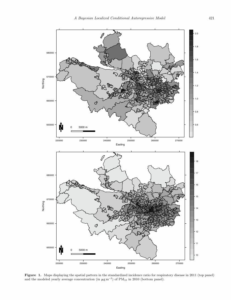
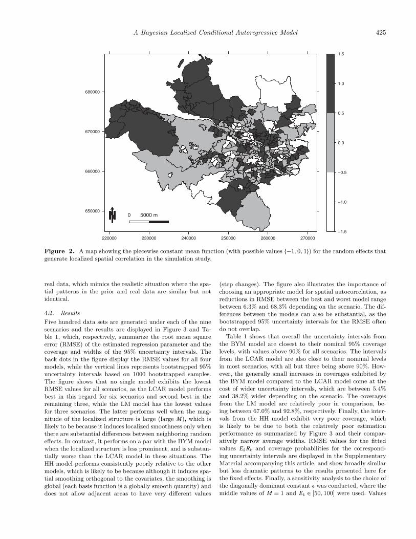
Simulated data are generated for the 271 IGs that comprisethe Greater Glasgow study region described in Section 2. Dis-ease counts are generated from model (1), where the size of theexpected numbers E is varied to assess its impact on modelperformance. The log risk surface is a linear combination of asingle spatially smooth covariate acting as air pollution, andlocalized residual spatial autocorrelation. The pollution co-variate is generated as the average of two Gaussian spatialprocesses with different ranges, one of which has the samerange and hence is confounded with the localized spatial au-tocorrelation. Both spatial processes are generated using theMatern family of correlation functions, where the smoothnessparameter equals 2.5. The regression coefficient for the covari-ate is fixed at β = 0.1, while new realizations of the covari-ate and the residual spatial autocorrelation are generated foreach simulated data set. The residual autocorrelation is alsogenerated from a Gaussian process with a Matern correlationfunction, where localized spatial structure is induced via apiecewise constant mean. The template for this is shown inFigure 2, and only has three distinct values {−1, 0, 1}. Thesevalues are multiplied by a constant M to obtain the expec-tation, where larger values of M lead to bigger step changesin the spatial surface. The study is split into nine differentscenarios comprising pairwise combinations of M = 0.5, 1, 1.5and Ek ∈ [10, 25], [50, 100], and [150, 200]. The size of E quan-tifies disease prevalence, while M determines the extent oflocal rather than global residual autocorrelation (larger val-ues correspond to more prominent localized structure). Eachsimulated data set consists of study data and 3 years of priordata, which is the number of prior data sets used in the Glas-gow motivating study. The residual spatial autocorrelationfor the latter is generated by adding uniform random noisein the range [−0.1, 0.1] to the realization generated for the

A Bayesian Localized Conditional Autoregressive Model 425

650000

660000

670000

680000

220000 230000 240000 250000 260000 270000

0 5000 m

−1.5

−1.0

−0.5

0.0

0.5

1.0

1.5

Figure 2. A map showing the piecewise constant mean function (with possible values {−1, 0, 1}) for the random effects thatgenerate localized spatial correlation in the simulation study.

real data, which mimics the realistic situation where the spa-tial patterns in the prior and real data are similar but notidentical.

4.2. Results

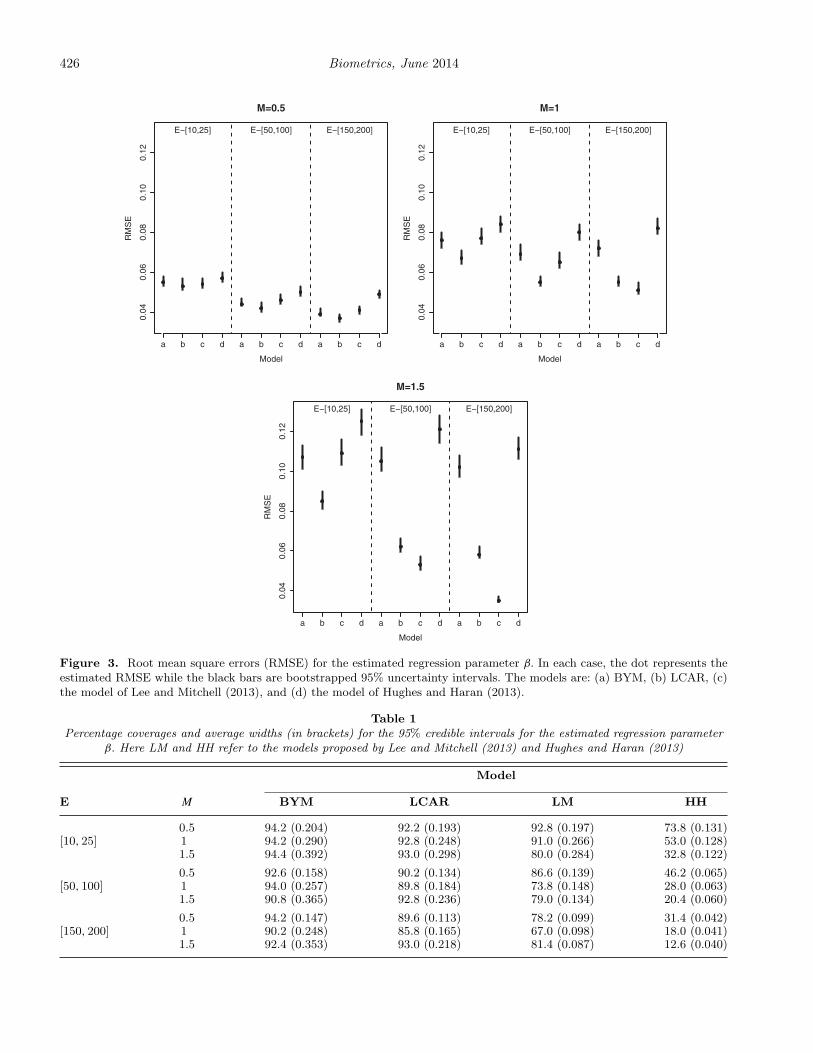
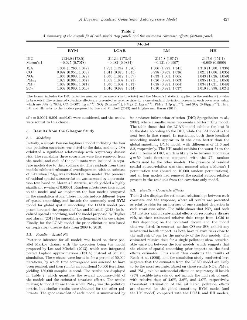
Five hundred data sets are generated under each of the ninescenarios and the results are displayed in Figure 3 and Ta-ble 1, which, respectively, summarize the root mean squareerror (RMSE) of the estimated regression parameter and thecoverage and widths of the 95% uncertainty intervals. Theback dots in the figure display the RMSE values for all fourmodels, while the vertical lines represents bootstrapped 95%uncertainty intervals based on 1000 bootstrapped samples.The figure shows that no single model exhibits the lowestRMSE values for all scenarios, as the LCAR model performsbest in this regard for six scenarios and second best in theremaining three, while the LM model has the lowest valuesfor three scenarios. The latter performs well when the mag-nitude of the localized structure is large (large M), which islikely to be because it induces localized smoothness only whenthere are substantial differences between neighboring randomeffects. In contrast, it performs on a par with the BYM modelwhen the localized structure is less prominent, and is substan-tially worse than the LCAR model in these situations. TheHH model performs consistently poorly relative to the othermodels, which is likely to be because although it induces spa-tial smoothing orthogonal to the covariates, the smoothing isglobal (each basis function is a globally smooth quantity) anddoes not allow adjacent areas to have very different values

(step changes). The figure also illustrates the importance ofchoosing an appropriate model for spatial autocorrelation, asreductions in RMSE between the best and worst model rangebetween 6.3% and 68.3% depending on the scenario. The dif-ferences between the models can also be substantial, as thebootstrapped 95% uncertainty intervals for the RMSE oftendo not overlap.

Table 1 shows that overall the uncertainty intervals fromthe BYM model are closest to their nominal 95% coveragelevels, with values above 90% for all scenarios. The intervalsfrom the LCAR model are also close to their nominal levelsin most scenarios, with all but three being above 90%. How-ever, the generally small increases in coverages exhibited bythe BYM model compared to the LCAR model come at thecost of wider uncertainty intervals, which are between 5.4%and 38.2% wider depending on the scenario. The coveragesfrom the LM model are relatively poor in comparison, be-ing between 67.0% and 92.8%, respectively. Finally, the inter-vals from the HH model exhibit very poor coverage, whichis likely to be due to both the relatively poor estimationperformance as summarized by Figure 3 and their compar-atively narrow average widths. RMSE values for the fittedvalues EkRk and coverage probabilities for the correspond-ing uncertainty intervals are displayed in the SupplementaryMaterial accompanying this article, and show broadly similarbut less dramatic patterns to the results presented here forthe fixed effects. Finally, a sensitivity analysis to the choice ofthe diagonally dominant constant ε was conducted, where themiddle values of M = 1 and Ek ∈ [50, 100] were used. Values

426 Biometrics, June 2014

0.04

0.06

0.08

0.10

0.12

M=0.5

Model

RM

SE

a b c d a b c d a b c d

E−[10,25] E−[50,100] E−[150,200]

0.04

0.06

0.08

0.10

0.12

M=1

Model

RM

SE

a b c d a b c d a b c d

E−[10,25] E−[50,100] E−[150,200]

0.04

0.06

0.08

0.10

0.12

M=1.5

Model

RM

SE

a b c d a b c d a b c d

E−[10,25] E−[50,100] E−[150,200]

Figure 3. Root mean square errors (RMSE) for the estimated regression parameter β. In each case, the dot represents theestimated RMSE while the black bars are bootstrapped 95% uncertainty intervals. The models are: (a) BYM, (b) LCAR, (c)the model of Lee and Mitchell (2013), and (d) the model of Hughes and Haran (2013).

Table 1Percentage coverages and average widths (in brackets) for the 95% credible intervals for the estimated regression parameter

β. Here LM and HH refer to the models proposed by Lee and Mitchell (2013) and Hughes and Haran (2013)

Model

E M BYM LCAR LM HH

0.5 94.2 (0.204) 92.2 (0.193) 92.8 (0.197) 73.8 (0.131)[10, 25] 1 94.2 (0.290) 92.8 (0.248) 91.0 (0.266) 53.0 (0.128)

1.5 94.4 (0.392) 93.0 (0.298) 80.0 (0.284) 32.8 (0.122)

0.5 92.6 (0.158) 90.2 (0.134) 86.6 (0.139) 46.2 (0.065)[50, 100] 1 94.0 (0.257) 89.8 (0.184) 73.8 (0.148) 28.0 (0.063)

1.5 90.8 (0.365) 92.8 (0.236) 79.0 (0.134) 20.4 (0.060)

0.5 94.2 (0.147) 89.6 (0.113) 78.2 (0.099) 31.4 (0.042)[150, 200] 1 90.2 (0.248) 85.8 (0.165) 67.0 (0.098) 18.0 (0.041)

1.5 92.4 (0.353) 93.0 (0.218) 81.4 (0.087) 12.6 (0.040)

A Bayesian Localized Conditional Autoregressive Model 427

Table 2A summary of the overall fit of each model (top panel) and the estimated covariate effects (bottom panel)

Model

BYM LCAR LM HH

DIC 2124.0 (178.5) 2112.4 (173.4) 2115.8 (167.7) 2467.6 (157.1)Moran’s I −0.025 (0.7078) −0.082 (0.9834) −0.121 (0.9997) −0.089 (0.9909)

JSA 1.304 (1.268, 1.342) 1.283 (1.247, 1.320) 1.306 (1.272, 1.341) 1.318 (1.300, 1.336)CO 0.997 (0.954, 1.038) 1.011 (0.973, 1.045) 0.998 (0.959, 1.036) 1.021 (1.006, 1.035)NO2 1.036 (0.998, 1.072) 1.040 (1.012, 1.067) 1.033 (1.003, 1.065) 1.043 (1.028, 1.059)PM2.5 1.029 (0.991, 1.067) 1.039 (1.007, 1.071) 1.026 (0.989, 1.063) 1.035 (1.021, 1.050)PM10 1.032 (0.994, 1.071) 1.040 (1.007, 1.073) 1.028 (0.993, 1.064) 1.034 (1.021, 1.048)SO2 1.009 (0.980, 1.040) 1.016 (0.989, 1.044) 1.010 (0.983, 1.037) 1.010 (0.998, 1.024)

The former includes the DIC (effective number of parameters in brackets) and the Moran’s I statistic applied to the residuals (p-valuein brackets). The estimated covariate effects are presented as relative risks for a one standard deviation increase in each covariates value,which are JSA (2.78%), CO (0.0076 mg m−3), NO2 (5.0�gm−3), PM2.5 (1.1�g m−3), PM10 (1.5� g m−3), and SO2 (0.48�g m−3). Here,LM and HH refer to the models proposed by Lee and Mitchell (2013) and Hughes and Haran (2013).

of ε = 0.0001, 0.001, and0.01 were considered, and the resultswere robust to this choice.

5. Results from the Glasgow Study

5.1. Modeling

Initially, a simple Poisson log-linear model including the fournon-pollution covariates was fitted to the data, and only JSAexhibited a significant relationship with respiratory diseaserisk. The remaining three covariates were thus removed fromthe model, and each of the pollutants were included in sepa-rate models due to their collinearity. The residuals from thesemodels exhibited substantial overdispersion, with an estimateof 3.47 when PM2.5 was included in the model. The presenceof residual spatial autocorrelation was assessed by a permuta-tion test based on Moran’s I statistic, which yielded a highlysignificant p-value of 0.00001. Random effects were thus addedto the model, and we implement the four models comparedin the simulation study. These models induce different typesof spatial smoothing, and include the commonly used BYMmodel for global spatial smoothing, the LCAR model pro-posed here and the proposal of Lee and Mitchell (2013) for lo-calized spatial smoothing, and the model proposed by Hughesand Haran (2013) for smoothing orthogonal to the covariates.Finally, for the LCAR model the prior elicitation was basedon respiratory disease data from 2008 to 2010.

5.2. Results – Model Fit

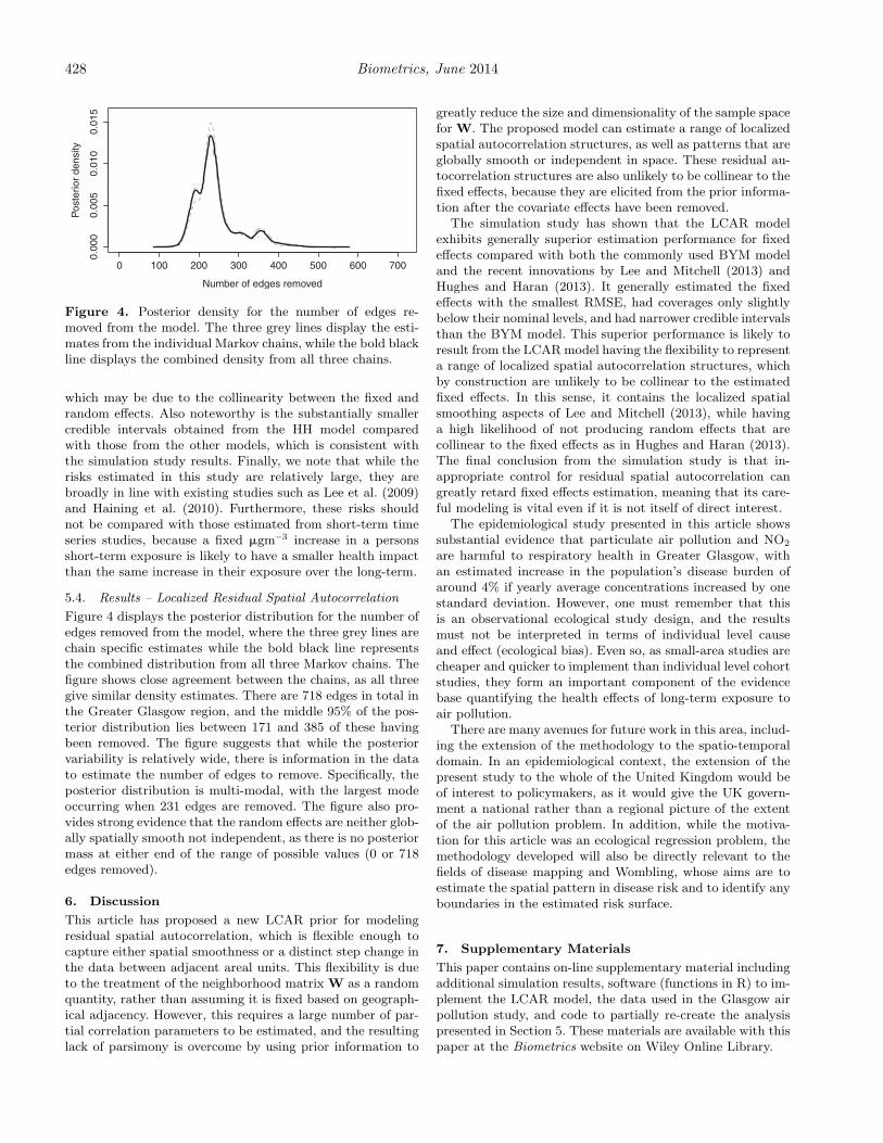
Posterior inference for all models was based on three par-allel Markov chains, with the exception being the modelproposed by Lee and Mitchell (2013), which uses integratednested Laplace approximations (INLA) instead of MCMCsimulation. These chains were burnt in for a period of 50,000iterations, by which time convergence was assessed to havebeen reached, and then run for an additional 50,000 iterations,yielding 150,000 samples in total. The results are displayedin Table 2, which quantifies the overall goodness-of-fit ofthe models and the estimated covariate effects. The resultsrelating to model fit are those where PM2.5 was the pollutionmetric, but similar results were obtained for the other pol-lutants. The goodness-of-fit of each model is summarized by

its deviance information criterion (DIC; Spiegelhalter et al.,2002), where a smaller value represents a better fitting model.The table shows that the LCAR model exhibits the best fitto the data according to the DIC, while the LM model is thenext best in that regard. In particular, both these localizedsmoothing models appear to fit the data better than theglobal smoothing BYM model, with differences of 11.6 and8.2, respectively. The HH model exhibits the worst fit to thedata in terms of DIC, which is likely to be because it containsq = 50 basis functions compared with the 271 randomeffects used by the other models. The presence of residualspatial autocorrelation was then assessed using a Moran’s Ipermutation test (based on 10,000 random permutations),and all four models had removed the spatial autocorrelationpresent in the residuals from the covariate only model.

5.3. Results – Covariate Effects

Table 2 also displays the estimated relationships between eachcovariate and the response, where all results are presentedas relative risks for an increase of one standard deviation ineach covariates value. The table shows that NO2 and bothPM metrics exhibit substantial effects on respiratory diseaserisk, as their estimated relative risks range from 1.026 to1.043 depending on the pollutant chosen and the modelthat was fitted. In contrast, neither CO nor SO2 exhibit anysubstantial health impact, as both have relative risks close tothe null risk of one for the majority of the four models. Theestimated relative risks for a single pollutant show consider-able variation between the four models, which suggests thatthe choice of spatial smoothing prior impacts on the fixedeffects estimates. This result thus confirms the results ofReich et al. (2006), and the simulation study conducted heresuggests that the estimates from the LCAR model are likelyto be the most accurate. Based on those results NO2, PM2.5,and PM10 exhibit substantial effects on respiratory ill health(95% credible intervals do not include the null risk of one),with relative risks of 4.0%, 3.9%, and 4.0%, respectively.Consistent attenuation of the estimated pollution effectsare observed for the global smoothing BYM model (andthe LM model) compared with the LCAR and HH models,

428 Biometrics, June 2014

0 100 200 300 400 500 600 700

0.00

00.

005

0.01

00.

015

Number of edges removed

Pos

terio

r de

nsity

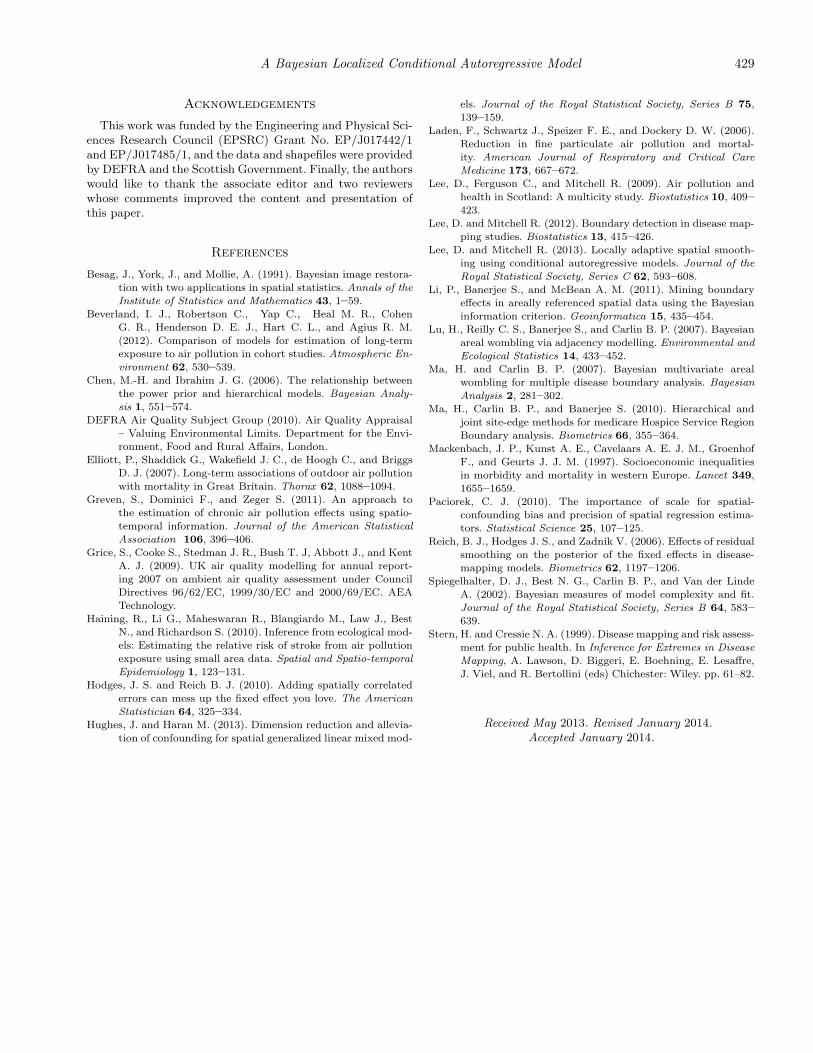
Figure 4. Posterior density for the number of edges re-moved from the model. The three grey lines display the esti-mates from the individual Markov chains, while the bold blackline displays the combined density from all three chains.

which may be due to the collinearity between the fixed andrandom effects. Also noteworthy is the substantially smallercredible intervals obtained from the HH model comparedwith those from the other models, which is consistent withthe simulation study results. Finally, we note that while therisks estimated in this study are relatively large, they arebroadly in line with existing studies such as Lee et al. (2009)and Haining et al. (2010). Furthermore, these risks shouldnot be compared with those estimated from short-term timeseries studies, because a fixed �gm−3 increase in a personsshort-term exposure is likely to have a smaller health impactthan the same increase in their exposure over the long-term.

5.4. Results – Localized Residual Spatial Autocorrelation

Figure 4 displays the posterior distribution for the number ofedges removed from the model, where the three grey lines arechain specific estimates while the bold black line representsthe combined distribution from all three Markov chains. Thefigure shows close agreement between the chains, as all threegive similar density estimates. There are 718 edges in total inthe Greater Glasgow region, and the middle 95% of the pos-terior distribution lies between 171 and 385 of these havingbeen removed. The figure suggests that while the posteriorvariability is relatively wide, there is information in the datato estimate the number of edges to remove. Specifically, theposterior distribution is multi-modal, with the largest modeoccurring when 231 edges are removed. The figure also pro-vides strong evidence that the random effects are neither glob-ally spatially smooth not independent, as there is no posteriormass at either end of the range of possible values (0 or 718edges removed).

6. Discussion

This article has proposed a new LCAR prior for modelingresidual spatial autocorrelation, which is flexible enough tocapture either spatial smoothness or a distinct step change inthe data between adjacent areal units. This flexibility is dueto the treatment of the neighborhood matrix W as a randomquantity, rather than assuming it is fixed based on geograph-ical adjacency. However, this requires a large number of par-tial correlation parameters to be estimated, and the resultinglack of parsimony is overcome by using prior information to

greatly reduce the size and dimensionality of the sample spacefor W. The proposed model can estimate a range of localizedspatial autocorrelation structures, as well as patterns that areglobally smooth or independent in space. These residual au-tocorrelation structures are also unlikely to be collinear to thefixed effects, because they are elicited from the prior informa-tion after the covariate effects have been removed.

The simulation study has shown that the LCAR modelexhibits generally superior estimation performance for fixedeffects compared with both the commonly used BYM modeland the recent innovations by Lee and Mitchell (2013) andHughes and Haran (2013). It generally estimated the fixedeffects with the smallest RMSE, had coverages only slightlybelow their nominal levels, and had narrower credible intervalsthan the BYM model. This superior performance is likely toresult from the LCAR model having the flexibility to representa range of localized spatial autocorrelation structures, whichby construction are unlikely to be collinear to the estimatedfixed effects. In this sense, it contains the localized spatialsmoothing aspects of Lee and Mitchell (2013), while havinga high likelihood of not producing random effects that arecollinear to the fixed effects as in Hughes and Haran (2013).The final conclusion from the simulation study is that in-appropriate control for residual spatial autocorrelation cangreatly retard fixed effects estimation, meaning that its care-ful modeling is vital even if it is not itself of direct interest.

The epidemiological study presented in this article showssubstantial evidence that particulate air pollution and NO2

are harmful to respiratory health in Greater Glasgow, withan estimated increase in the population’s disease burden ofaround 4% if yearly average concentrations increased by onestandard deviation. However, one must remember that thisis an observational ecological study design, and the resultsmust not be interpreted in terms of individual level causeand effect (ecological bias). Even so, as small-area studies arecheaper and quicker to implement than individual level cohortstudies, they form an important component of the evidencebase quantifying the health effects of long-term exposure toair pollution.

There are many avenues for future work in this area, includ-ing the extension of the methodology to the spatio-temporaldomain. In an epidemiological context, the extension of thepresent study to the whole of the United Kingdom would beof interest to policymakers, as it would give the UK govern-ment a national rather than a regional picture of the extentof the air pollution problem. In addition, while the motiva-tion for this article was an ecological regression problem, themethodology developed will also be directly relevant to thefields of disease mapping and Wombling, whose aims are toestimate the spatial pattern in disease risk and to identify anyboundaries in the estimated risk surface.

7. Supplementary Materials

This paper contains on-line supplementary material includingadditional simulation results, software (functions in R) to im-plement the LCAR model, the data used in the Glasgow airpollution study, and code to partially re-create the analysispresented in Section 5. These materials are available with thispaper at the Biometrics website on Wiley Online Library.

A Bayesian Localized Conditional Autoregressive Model 429

Acknowledgements

This work was funded by the Engineering and Physical Sci-ences Research Council (EPSRC) Grant No. EP/J017442/1and EP/J017485/1, and the data and shapefiles were providedby DEFRA and the Scottish Government. Finally, the authorswould like to thank the associate editor and two reviewerswhose comments improved the content and presentation ofthis paper.

References

Besag, J., York, J., and Mollie, A. (1991). Bayesian image restora-tion with two applications in spatial statistics. Annals of theInstitute of Statistics and Mathematics 43, 1–59.

Beverland, I. J., Robertson C., Yap C., Heal M. R., CohenG. R., Henderson D. E. J., Hart C. L., and Agius R. M.(2012). Comparison of models for estimation of long-termexposure to air pollution in cohort studies. Atmospheric En-vironment 62, 530–539.

Chen, M.-H. and Ibrahim J. G. (2006). The relationship betweenthe power prior and hierarchical models. Bayesian Analy-sis 1, 551–574.

DEFRA Air Quality Subject Group (2010). Air Quality Appraisal– Valuing Environmental Limits. Department for the Envi-ronment, Food and Rural Affairs, London.

Elliott, P., Shaddick G., Wakefield J. C., de Hoogh C., and BriggsD. J. (2007). Long-term associations of outdoor air pollutionwith mortality in Great Britain. Thorax 62, 1088–1094.

Greven, S., Dominici F., and Zeger S. (2011). An approach tothe estimation of chronic air pollution effects using spatio-temporal information. Journal of the American StatisticalAssociation 106, 396–406.

Grice, S., Cooke S., Stedman J. R., Bush T. J, Abbott J., and KentA. J. (2009). UK air quality modelling for annual report-ing 2007 on ambient air quality assessment under CouncilDirectives 96/62/EC, 1999/30/EC and 2000/69/EC. AEATechnology.

Haining, R., Li G., Maheswaran R., Blangiardo M., Law J., BestN., and Richardson S. (2010). Inference from ecological mod-els: Estimating the relative risk of stroke from air pollutionexposure using small area data. Spatial and Spatio-temporalEpidemiology 1, 123–131.

Hodges, J. S. and Reich B. J. (2010). Adding spatially correlatederrors can mess up the fixed effect you love. The AmericanStatistician 64, 325–334.

Hughes, J. and Haran M. (2013). Dimension reduction and allevia-tion of confounding for spatial generalized linear mixed mod-

els. Journal of the Royal Statistical Society, Series B 75,139–159.

Laden, F., Schwartz J., Speizer F. E., and Dockery D. W. (2006).Reduction in fine particulate air pollution and mortal-ity. American Journal of Respiratory and Critical CareMedicine 173, 667–672.

Lee, D., Ferguson C., and Mitchell R. (2009). Air pollution andhealth in Scotland: A multicity study. Biostatistics 10, 409–423.

Lee, D. and Mitchell R. (2012). Boundary detection in disease map-ping studies. Biostatistics 13, 415–426.

Lee, D. and Mitchell R. (2013). Locally adaptive spatial smooth-ing using conditional autoregressive models. Journal of theRoyal Statistical Society, Series C 62, 593–608.

Li, P., Banerjee S., and McBean A. M. (2011). Mining boundaryeffects in areally referenced spatial data using the Bayesianinformation criterion. Geoinformatica 15, 435–454.

Lu, H., Reilly C. S., Banerjee S., and Carlin B. P. (2007). Bayesianareal wombling via adjacency modelling. Environmental andEcological Statistics 14, 433–452.

Ma, H. and Carlin B. P. (2007). Bayesian multivariate arealwombling for multiple disease boundary analysis. BayesianAnalysis 2, 281–302.

Ma, H., Carlin B. P., and Banerjee S. (2010). Hierarchical andjoint site-edge methods for medicare Hospice Service RegionBoundary analysis. Biometrics 66, 355–364.

Mackenbach, J. P., Kunst A. E., Cavelaars A. E. J. M., GroenhofF., and Geurts J. J. M. (1997). Socioeconomic inequalitiesin morbidity and mortality in western Europe. Lancet 349,1655–1659.

Paciorek, C. J. (2010). The importance of scale for spatial-confounding bias and precision of spatial regression estima-tors. Statistical Science 25, 107–125.

Reich, B. J., Hodges J. S., and Zadnik V. (2006). Effects of residualsmoothing on the posterior of the fixed effects in disease-mapping models. Biometrics 62, 1197–1206.

Spiegelhalter, D. J., Best N. G., Carlin B. P., and Van der LindeA. (2002). Bayesian measures of model complexity and fit.Journal of the Royal Statistical Society, Series B 64, 583–639.

Stern, H. and Cressie N. A. (1999). Disease mapping and risk assess-ment for public health. In Inference for Extremes in DiseaseMapping, A. Lawson, D. Biggeri, E. Boehning, E. Lesaffre,J. Viel, and R. Bertollini (eds) Chichester: Wiley. pp. 61–82.

Received May 2013. Revised January 2014.Accepted January 2014.