A Bayesian Level-k Model in n-Person Games

Teck-Hua Ho, So-Eun Park, and Xuanming Su ∗

March 19, 2015

In standard models of iterative thinking, players choose a fixed rule

level from a fixed rule hierarchy. Nonequilibrium behavior emerges when

players do not perform enough thinking steps. Existing approaches, how-

ever, are inherently static. This paper introduces a Bayesian level-k

model, in which players perform Bayesian updating of their beliefs on

opponents’ rule levels and best-respond with different rule levels over

time. In this way, players exhibit sophisticated learning. We apply

our model to experimental data on p-beauty contest and price matching

games. We find that it is crucial to incorporate sophisticated learning

to explain dynamic choice behavior.

Over the past few decades, accumulating evidence from laboratory and field

experiments has shown that players’ actual behavior may significantly devi-

ate from the equilibrium solution in a systematic manner. That is, despite

nontrivial financial incentives, subjects frequently do not play the equilibrium

solution. For example, the first round offer in sequential bargaining games

often neither corresponds to the equilibrium offer nor is accepted immediately

(Binmore, Shaked and Sutton, 1985; Ochs and Roth, 1989); centipede games

often proceed to intermediate stages rather than end immediately (McKelvey

and Palfrey, 1992); and many players do not choose the unique iterative dom-

inance solution in dominance solvable games (Nagel, 1995; Stahl and Wilson,

∗Ho: University of California, Berkeley and National University of Singapore, 2220Piedmont Avenue, Berkeley, CA 94720, hoteck@haas.berkeley.edu. Park: Universityof British Columbia, 2053 Main Mall, Vancouver, British Columbia V6T1Z2 Canada,soeun.park@sauder.ubc.ca. Su: University of Pennsylvania, 3620 Walnut Street, Philadel-phia, PA 19104, xuanming@wharton.upenn.edu. Authors are listed in alphabetical order.Direct correspondence to any of the authors. We thank Colin Camerer, Vince Crawford,David Levine, and seminar participants at National University of Singapore, University ofBritish Columbia and University of California, Berkeley for their helpful comments.

1

1994, 1995; Ho et al., 1998; Costa-Gomes et al., 2001; Bosch-Domenech et al.,

2002; Costa-Gomes and Crawford, 2006; Costa-Gomes and Weizsacker, 2008).

To explain nonequilibrium behavior in games, cognitive hierarchy (Camerer

et al., 2004) and level-k (Nagel, 1995; Stahl and Wilson, 1994, 1995; Costa-

Gomes et al., 2001; Costa-Gomes et al., 2009; Costa-Gomes and Crawford,

2006; Crawford, 2003; Crawford and Iriberri, 2007b) models have developed;

for a comprehensive review, see Crawford et al., 2013. These models assume

that players choose rules from a well-defined discrete rule hierarchy. The rule

hierarchy is defined iteratively by assuming that a level-k rule best-responds

to a lower level rule (e.g., level-(k − 1) where k ≥ 1). The level-0 rule can be

specified a priori either as uniform randomization among all possible strategies

or as the most salient action derived from the payoff structure.1 Let us illus-

trate how to apply these models using two examples: p-beauty contest and

traveler’s dilemma games.

• In the p-beauty contest game, n players simultaneously choose numbers

ranging from 0 to 100. The winner is the player who chose the number closest

to the target number, defined as p times the average of all chosen numbers,

where 0 < p < 1. A fixed reward goes to the winner, and it is divided evenly

among winners in the case of a tie. This game is dominance-solvable and the

unique number that survives the iterative elimination process is 0.2 To apply

1The level-k and cognitive hierarchy models have also been applied to study games withasymmetric information such as zero-sum betting, auctions and strategic information dis-closure (e.g., Camerer et al., 2004; Crawford and Iriberri, 2007a.; Brocas et al., 2010; Brown

et al., 2010; Ostling et al., 2011). Crawford et al. (2009) employ level-k models to deter-mine the optimal design for auctions when bidders are boundedly rational. Goldfarb andYang (2009) and Goldfarb and Xiao (2011) apply the cognitive hierarchy model to captureheterogeneity in the abilities of firms or managers, and use it to predict a firm’s long-termsuccess in oligopolistic markets.

2To illustrate, let us assume p = 0.7. Strategies between 70 and 100 are weakly domi-nated by 70 and thus are eliminated at the first step of elimination of dominated strategies.Likewise, strategies between 49 and 70 are eliminated at the second step of elimination asthey are weakly dominated by 49. Ultimately, the only strategy that survives the iterativeelimination of dominated strategies is zero, which is the unique iterative dominance solutionof the game.

2

the standard level-k model, assume that the level-0 rule randomizes between

all possible choices between 0 and 100 and thus chooses 50 on average. Best-

responding to the level-0 opponents, the level-1 rule seeks to hit the target

number in order to maximize the payoff. Specifically, the level-1 rule chooses

x∗ = p · x∗+(n−1)·50n

as a best response to its level-0 opponents, taking into

account her own influence on the group mean.3 Proceeding iteratively, a

level-k rule will choose(

p·(n−1)n−p

)k

· 50, which converges to 0 as k increases.

• In the traveler’s dilemma game, two travelers whose identical antiques were

damaged by an airline were promised compensation according to the fol-

lowing scheme. Both travelers were asked to privately declare the value xi

of the antique as any integer dollar between $2 and $100. They were then

compensated the lower declared value, mini xi. In addition, the traveler who

declared the lower value is rewarded with $2 (i.e., he receives mini xi + 2),

while the other traveler who declared a higher value is penalized with $2

(i.e., he receives mini xi − 2). If both give the same value, they receive

neither reward nor penalty (i.e., they both receive mini xi). This traveler’s

dilemma game can also be interpreted as a price matching (i.e., lowest price

guarantee) game between two firms selling an identical product. The firm

charging the lower price is rewarded with customer satisfaction while the

firm charging the higher price is punished with customer dissatisfaction.4

In this game, the unique iterative dominance solution is 2; in general, it is

the lower corner of the strategy space.5 To apply the level-k model, we as-

3Some prior research (e.g., Nagel, 1995) ignores one’s own influence on the group averageby simply assuming that the level-1 rule chooses p · 50 and the level-k rule chooses pk · 50.This approximation is good only when n is large. For example, when n = 100, the level-1rule’s exact best response is 34.89, which is close to 35.

4Price matching is common in the retail industry. Marketing researchers (Jain andSrivastava, 2000; Chen et al., 2001; Srivastava and Lurie, 2001) suggest that firms whichpromise to charge the lowest price are perceived negatively if customers find out that thefirms’ prices are not the lowest.

5At the first step of elimination of dominated strategies, 99 and 100 are eliminated sincethey are dominated by 98. At the second step of elimination, 97 and 98 are eliminated beingdominated by 96. Hence, the strategy that ultimately survives the iterative elimination of

3

sume that the level-0 rule naıvely declares the true value, say 51. Then, the

level-1 rule chooses the payoff maximizing strategy, which is 50 = 51 − 1,

receiving a payoff of 52. Proceeding iteratively, the level-k rule chooses

max{51− k, 2}, which converges to the equilibrium 2 as k increases.

In both games, nonequilibrium behavior emerges when players do not per-

form enough thinking steps. Beyond these two examples, level-k models have

also been used to explain nonequilibrium behavior in applications including

auctions (Crawford and Iriberri, 2007b), matrix games (Costa-Gomes et al.,

2001), and signaling games (Brown et al., 2012).6

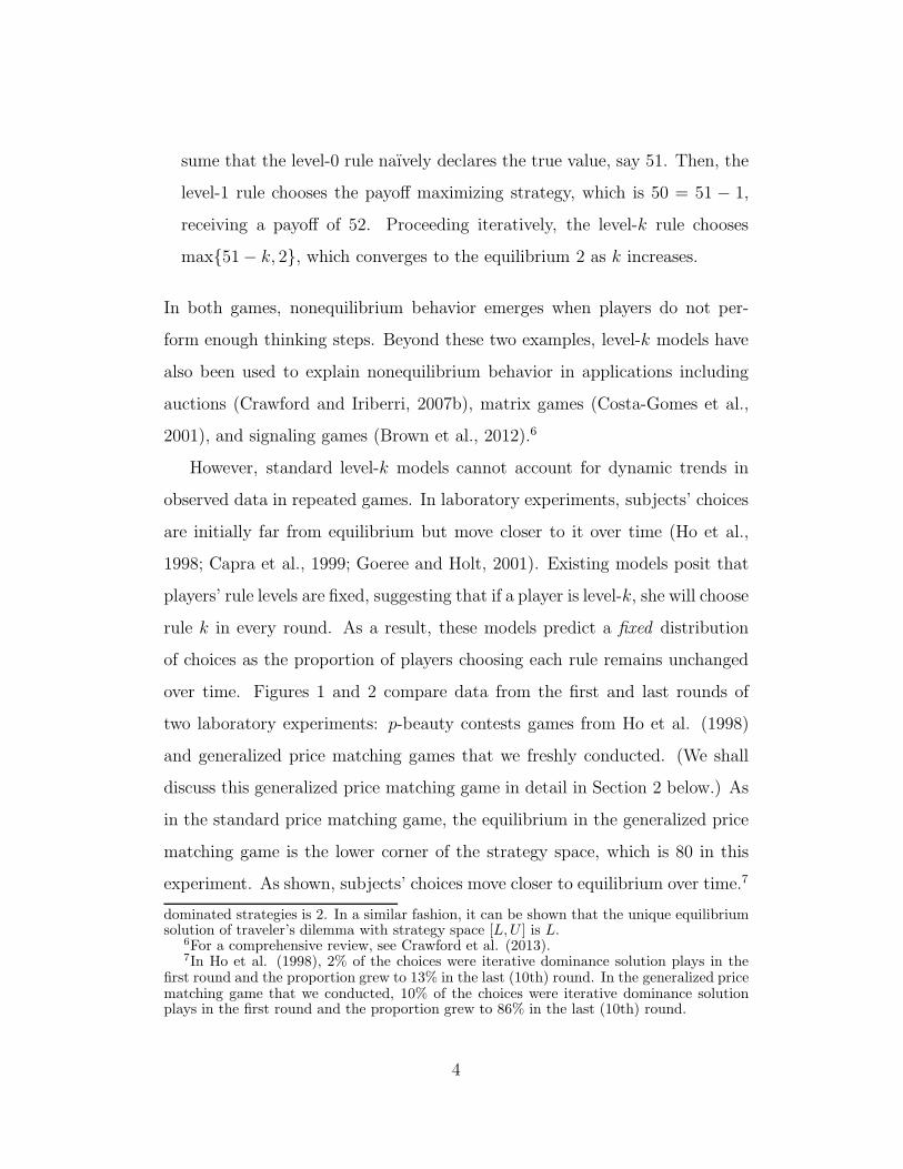
However, standard level-k models cannot account for dynamic trends in

observed data in repeated games. In laboratory experiments, subjects’ choices

are initially far from equilibrium but move closer to it over time (Ho et al.,

1998; Capra et al., 1999; Goeree and Holt, 2001). Existing models posit that

players’ rule levels are fixed, suggesting that if a player is level-k, she will choose

rule k in every round. As a result, these models predict a fixed distribution

of choices as the proportion of players choosing each rule remains unchanged

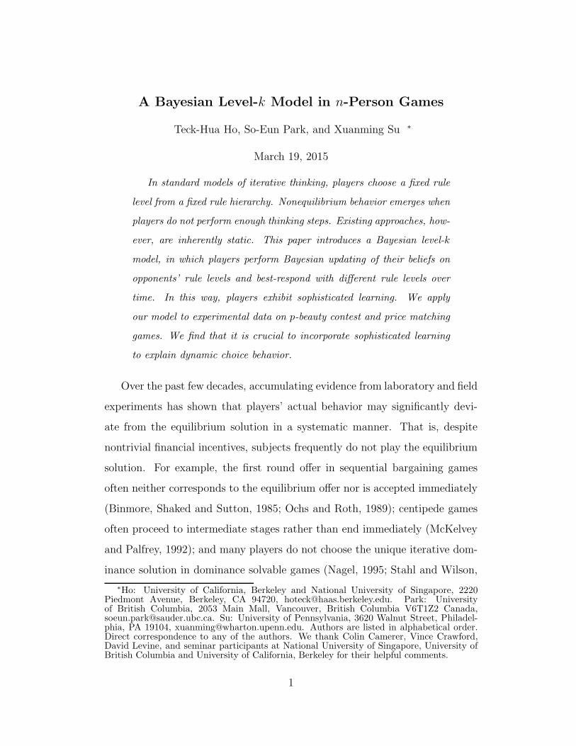
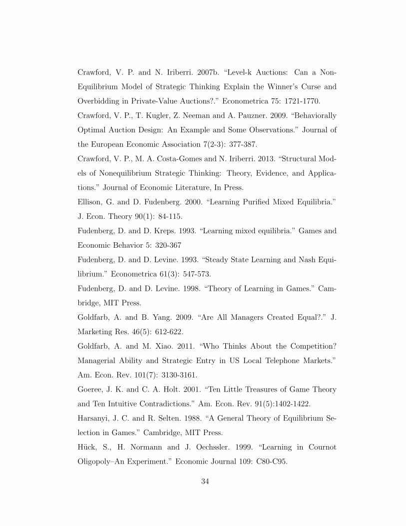
over time. Figures 1 and 2 compare data from the first and last rounds of

two laboratory experiments: p-beauty contests games from Ho et al. (1998)

and generalized price matching games that we freshly conducted. (We shall

discuss this generalized price matching game in detail in Section 2 below.) As

in the standard price matching game, the equilibrium in the generalized price

matching game is the lower corner of the strategy space, which is 80 in this

experiment. As shown, subjects’ choices move closer to equilibrium over time.7

dominated strategies is 2. In a similar fashion, it can be shown that the unique equilibriumsolution of traveler’s dilemma with strategy space [L,U ] is L.

6For a comprehensive review, see Crawford et al. (2013).7In Ho et al. (1998), 2% of the choices were iterative dominance solution plays in the

first round and the proportion grew to 13% in the last (10th) round. In the generalized pricematching game that we conducted, 10% of the choices were iterative dominance solutionplays in the first round and the proportion grew to 86% in the last (10th) round.

4

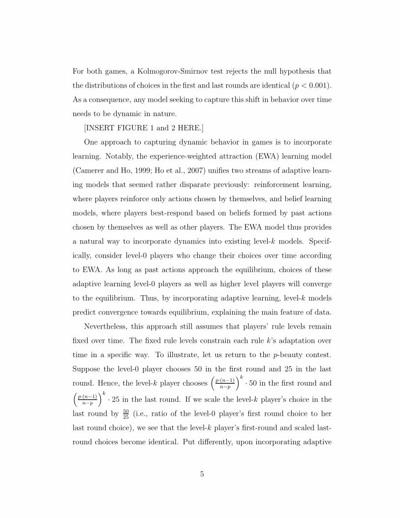
For both games, a Kolmogorov-Smirnov test rejects the null hypothesis that

the distributions of choices in the first and last rounds are identical (p < 0.001).

As a consequence, any model seeking to capture this shift in behavior over time

needs to be dynamic in nature.

[INSERT FIGURE 1 and 2 HERE.]

One approach to capturing dynamic behavior in games is to incorporate

learning. Notably, the experience-weighted attraction (EWA) learning model

(Camerer and Ho, 1999; Ho et al., 2007) unifies two streams of adaptive learn-

ing models that seemed rather disparate previously: reinforcement learning,

where players reinforce only actions chosen by themselves, and belief learning

models, where players best-respond based on beliefs formed by past actions

chosen by themselves as well as other players. The EWA model thus provides

a natural way to incorporate dynamics into existing level-k models. Specif-

ically, consider level-0 players who change their choices over time according

to EWA. As long as past actions approach the equilibrium, choices of these

adaptive learning level-0 players as well as higher level players will converge

to the equilibrium. Thus, by incorporating adaptive learning, level-k models

predict convergence towards equilibrium, explaining the main feature of data.

Nevertheless, this approach still assumes that players’ rule levels remain

fixed over time. The fixed rule levels constrain each rule k’s adaptation over

time in a specific way. To illustrate, let us return to the p-beauty contest.

Suppose the level-0 player chooses 50 in the first round and 25 in the last

round. Hence, the level-k player chooses(

p·(n−1)n−p

)k

· 50 in the first round and(

p·(n−1)n−p

)k

· 25 in the last round. If we scale the level-k player’s choice in the

last round by 5025

(i.e., ratio of the level-0 player’s first round choice to her

last round choice), we see that the level-k player’s first-round and scaled last-

round choices become identical. Put differently, upon incorporating adaptive

5

learning, existing level-k models make a sharp prediction: the distributions

of first-round and scaled last-round choices are identical. We can readily test

this sharp prediction using data from p-beauty contest and generalized price

matching games. In both games, a Kolmogorov-Smirnov test rejects the null

hypothesis that the first-round and scaled last-round choices come from the

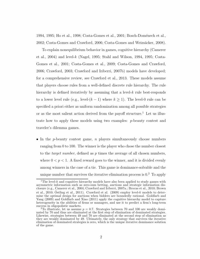
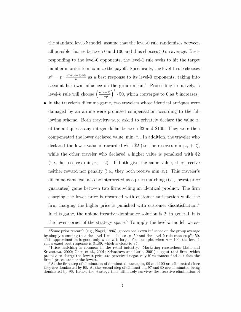
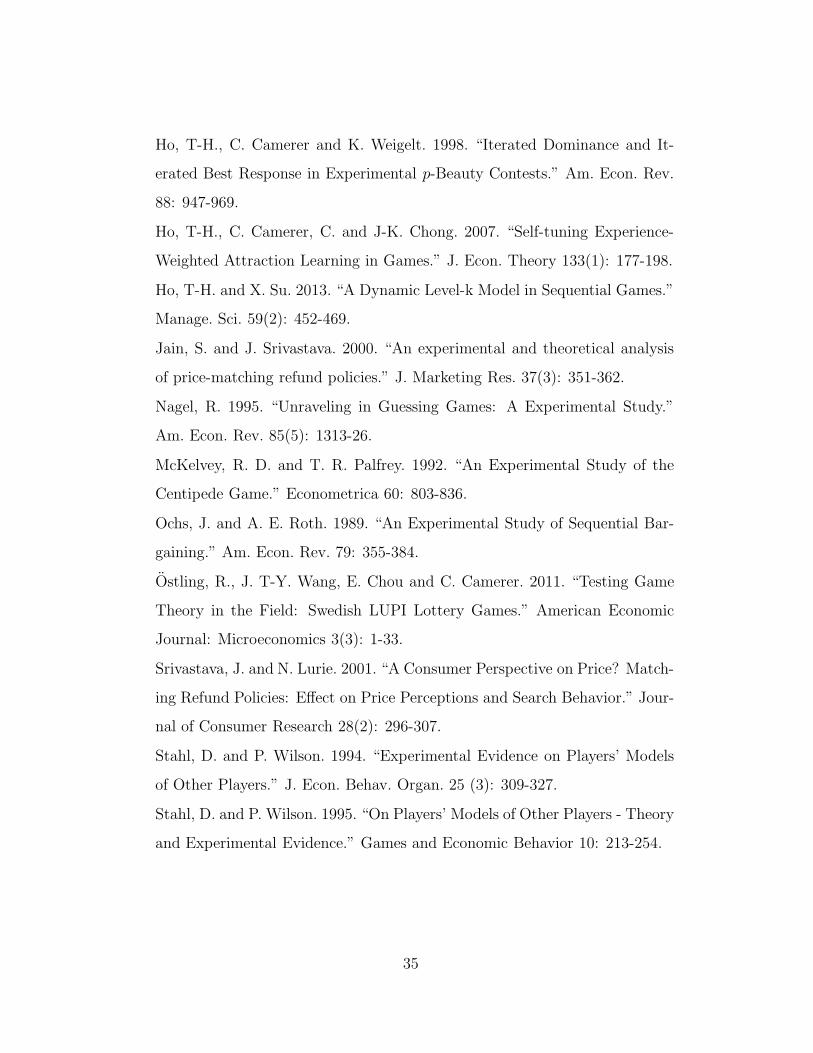
same distribution (p < 0.001). Figures 3 and 4 show the distributions of the

first-round, last-round, and scaled last-round choices in p-beauty contest and

generalized price matching games, respectively. Contrary to the prediction of

existing level-k models, the distribution of scaled last-round choices is to the

left of that of first-round choices in both games, suggesting that players choose

higher level rules in the last round than in the first round and that adaptive

learning models under-predict the speed of convergence towards equilibrium.

[INSERT FIGURE 3 and 4 HERE.]

A sensible way to account for the systematic shift in players’ scaled choices

is to allow players to become more sophisticated (i.e., change their rule levels)

over time. Specifically, in our model, players are assumed to form beliefs about

what rules opponents are likely to use, update their beliefs after each round

via Bayesian updating based on their observations, and best-respond to their

updated beliefs in the subsequent round. Consequently, the distribution of

players’ rule levels changes over time. To the extent that players move up the

rule hierarchy over time, this Bayesian level-k model will be able to explain

the leftward shift of the scaled last round choices.

In this paper, we propose a model that generalizes the standard level-k

model. This model holds three key features:

1. Our model is general and applicable to any n-person game that has a well-

defined rule hierarchy.

2. Our model nests existing nonequilibrium models such as EWA learning,

6

imitation learning and level-k models, and may serve as a model of equili-

bration process.

3. Players’ rule levels are dynamic in that players perform Bayesian updating

of their beliefs about opponents’ rule levels and thus may adopt different

rules over time.

We apply our proposed model to experimental data from two dominance-

solvable games: p-beauty contest and generalized price matching. Estimation

results show that our model describes subjects’ dynamic behavior better than

all its special cases. We find that it is crucial to incorporate sophisticated

learning even after other existing nonequilibrium models are introduced.

The rest of the paper is organized as follows. Section 1 formulates the

general model and its special cases. Section 2 applies the model to both p-

beauty contest and generalized price matching games, and presents empirical

results from the best fitting model and its special cases. Section 3 concludes.

1 Bayesian Level-k Model

1.1 Notation

We consider the class of n-player games. Players are indexed by i (i =

1, 2, . . . , n). Player i’s strategy space is denoted by Si, which can be ei-

ther discrete or continuous. Players play the game repeatedly for a total of

T rounds. Player i’s chosen action at time t is denoted by xi(t) ∈ Si. The vec-

tor of all players’ actions at time t excluding player i’s is denoted by x−i(t) =

(x1(t), . . . , xi−1(t), xi+1(t), . . . , xn(t)). Player i’s best response function given

her prediction of opponents’ actions is denoted by BRi(·) : (S1 × · · · × Si−1×

Si+1 × · · · × Sn) → Si.

7

1.2 Rule Hierarchy

Players choose rules k ∈ Z0+ = {0, 1, 2, . . .} from iteratively-defined discrete

rule hierarchies, and choose actions corresponding to these rules. Each player

has her own rule hierarchy, and each rule hierarchy is iteratively defined such

that a level-(k + 1) rule is a best response to the opponents’ level-k rules

(Stahl and Wilson, 1994; Nagel, 1995; Ho et al., 1998; Crawford et al., 2013).

In symmetric n-player games, all players’ rule hierarchies are identical, but

they may not be in general.

Let ki(t) be player i’s chosen rule and aki(t)i (t) ∈ Si be the action corre-

sponding to rule ki(t) under player i’s rule hierarchy at time t. Below we

discuss how player i chooses ki(t) and how aki(t)i (t) varies over time as the

game evolves.

1.3 Belief Draw and Best Response

Players have beliefs about what rule levels their opponents will choose at time t.

Denote player i’s belief at the end of time t byBi(t) = (B0i (t), B

1i (t), B

2i (t), . . .),

where Bki (t) refers to the probability that player i’s opponents will choose

rule k in the next time period. Based on Bi(t), player i conducts a single

draw di(t + 1) from {0, 1, 2, . . .} with probability Bdi(t+1)i (t) at the beginning

of time t + 1.8 Player i then conjectures that all her opponents will choose

rule di(t + 1) at time t + 1. Put differently, player i predicts that all her

opponents j (∀j 6= i) will choose the action adi(t+1)j (t+ 1) that corresponds to

rule di(t+ 1) at time t+ 1.

Player i then best-responds to this prediction by choosing:

8In a 2-person game, a single draw assumption is reasonable. In an n-player game,players might conduct multiple draws, perhaps one draw per opponent. If this is indeed thecase, each player conducts a separate draw for each opponent and each draw comes froma separate distribution. Prior research suggests that this is unlikely to be true. In fact,opponents’ choices are found to be often perfectly correlated (Ho et al. (1998)) and playerstend to treat all their opponents as an aggregate player.

8

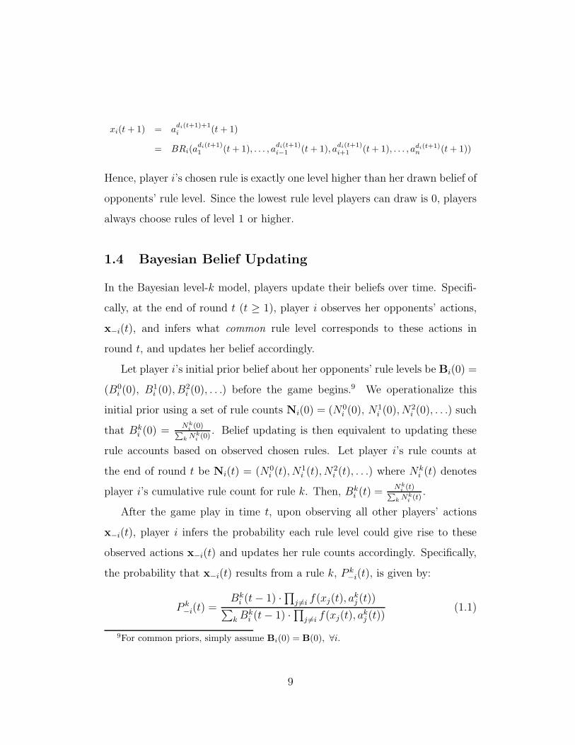
xi(t+ 1) = adi(t+1)+1i

(t+ 1)

= BRi(adi(t+1)1 (t+ 1), . . . , a

di(t+1)i−1 (t+ 1), a

di(t+1)i+1 (t+ 1), . . . , adi(t+1)

n(t+ 1))

Hence, player i’s chosen rule is exactly one level higher than her drawn belief of

opponents’ rule level. Since the lowest rule level players can draw is 0, players

always choose rules of level 1 or higher.

1.4 Bayesian Belief Updating

In the Bayesian level-k model, players update their beliefs over time. Specifi-

cally, at the end of round t (t ≥ 1), player i observes her opponents’ actions,

x−i(t), and infers what common rule level corresponds to these actions in

round t, and updates her belief accordingly.

Let player i’s initial prior belief about her opponents’ rule levels be Bi(0) =

(B0i (0), B1

i (0), B2i (0), . . .) before the game begins.9 We operationalize this

initial prior using a set of rule counts Ni(0) = (N0i (0), N

1i (0), N

2i (0), . . .) such

that Bki (0) =

Nki (0)

∑

k Nki (0)

. Belief updating is then equivalent to updating these

rule accounts based on observed chosen rules. Let player i’s rule counts at

the end of round t be Ni(t) = (N0i (t), N

1i (t), N

2i (t), . . .) where Nk

i (t) denotes

player i’s cumulative rule count for rule k. Then, Bki (t) =

Nki (t)

∑

k Nki (t)

.

After the game play in time t, upon observing all other players’ actions

x−i(t), player i infers the probability each rule level could give rise to these

observed actions x−i(t) and updates her rule counts accordingly. Specifically,

the probability that x−i(t) results from a rule k, P k−i(t), is given by:

P k−i(t) =

Bki (t− 1) ·

∏

j 6=i f(xj(t), akj (t))

∑

k Bki (t− 1) ·

∏

j 6=i f(xj(t), akj (t))

(1.1)

9For common priors, simply assume Bi(0) = B(0), ∀i.

9

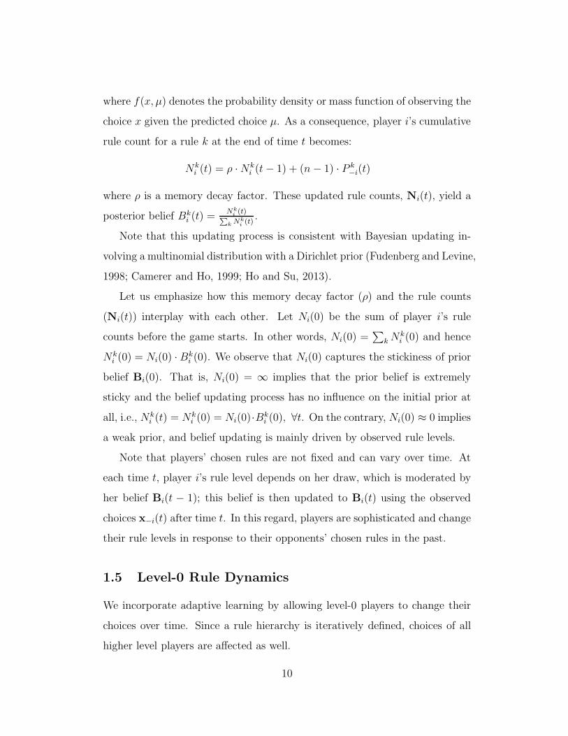
where f(x, µ) denotes the probability density or mass function of observing the

choice x given the predicted choice µ. As a consequence, player i’s cumulative

rule count for a rule k at the end of time t becomes:

Nki (t) = ρ ·Nk

i (t− 1) + (n− 1) · P k−i(t)

where ρ is a memory decay factor. These updated rule counts, Ni(t), yield a

posterior belief Bki (t) =

Nki (t)

∑

k Nki (t)

.

Note that this updating process is consistent with Bayesian updating in-

volving a multinomial distribution with a Dirichlet prior (Fudenberg and Levine,

1998; Camerer and Ho, 1999; Ho and Su, 2013).

Let us emphasize how this memory decay factor (ρ) and the rule counts

(Ni(t)) interplay with each other. Let Ni(0) be the sum of player i’s rule

counts before the game starts. In other words, Ni(0) =∑

k Nki (0) and hence

Nki (0) = Ni(0) · Bk

i (0). We observe that Ni(0) captures the stickiness of prior

belief Bi(0). That is, Ni(0) = ∞ implies that the prior belief is extremely

sticky and the belief updating process has no influence on the initial prior at

all, i.e., Nki (t) = Nk

i (0) = Ni(0)·Bki (0), ∀t. On the contrary, Ni(0) ≈ 0 implies

a weak prior, and belief updating is mainly driven by observed rule levels.

Note that players’ chosen rules are not fixed and can vary over time. At

each time t, player i’s rule level depends on her draw, which is moderated by

her belief Bi(t − 1); this belief is then updated to Bi(t) using the observed

choices x−i(t) after time t. In this regard, players are sophisticated and change

their rule levels in response to their opponents’ chosen rules in the past.

1.5 Level-0 Rule Dynamics

We incorporate adaptive learning by allowing level-0 players to change their

choices over time. Since a rule hierarchy is iteratively defined, choices of all

higher level players are affected as well.

10

We introduce heterogeneity to the types of players. Specifically, we let

a player be a level-0, adaptive learning player throughout the game with an

α probability; and be a belief-updating, sophisticated player throughout the

game with a 1− α probability. Put differently, with an α probability, player i

adopts rule 0 in every round and thus chooses a0i (t) in round t. On the other

hand, with a 1−α probability, player i undertakes sophisticated learning. That

is, she starts the game with an initial prior belief, updates her belief after each

round, conducts a single draw to predict which rule others will choose, and

best-responds accordingly. Note that by setting α = 1, our model reduces to

a pure adaptive learning model.

Incorporating adaptive learning into the Bayesian level-k model serves two

purposes. First, it unifies the existing wide stream of research on adaptive

learning since any adaptive learning model can be integrated as level-0 players’

behavior in our model. Second, it helps us to empirically control for the

potential existence of adaptive learning and hence tease out the respective roles

of adaptive and sophisticated learning in describing players’ choice dynamics.

1.6 Model Summary

The Bayesian level-k model (BLk(t)) exhibits the following key features:

1. (Belief Draw and Best Response) At the beginning of round t, player i

draws a belief di(t) from {0, 1, 2, . . .} with probability Bdi(t)i (t−1). Player i

then conjectures that all her opponents will choose rule di(t), i.e., x−i(t) =

(adi(t)1 (t), . . . , a

di(t)i−1 (t), a

di(t)i+1 (t), . . . , a

di(t)n (t)). Consequently, player i best-

responds in round t by choosing xi(t) = adi(t)+1i (t) = BRi(a

di(t)1 (t), . . . , a

di(t)i−1 (t),

adi(t)i+1 (t), . . . , a

di(t)n (t)).

2. (Belief Updating) At the end of round t, player i’s belief about her op-

ponents’ rule levels may change. Specifically, rule counts are updated af-

11

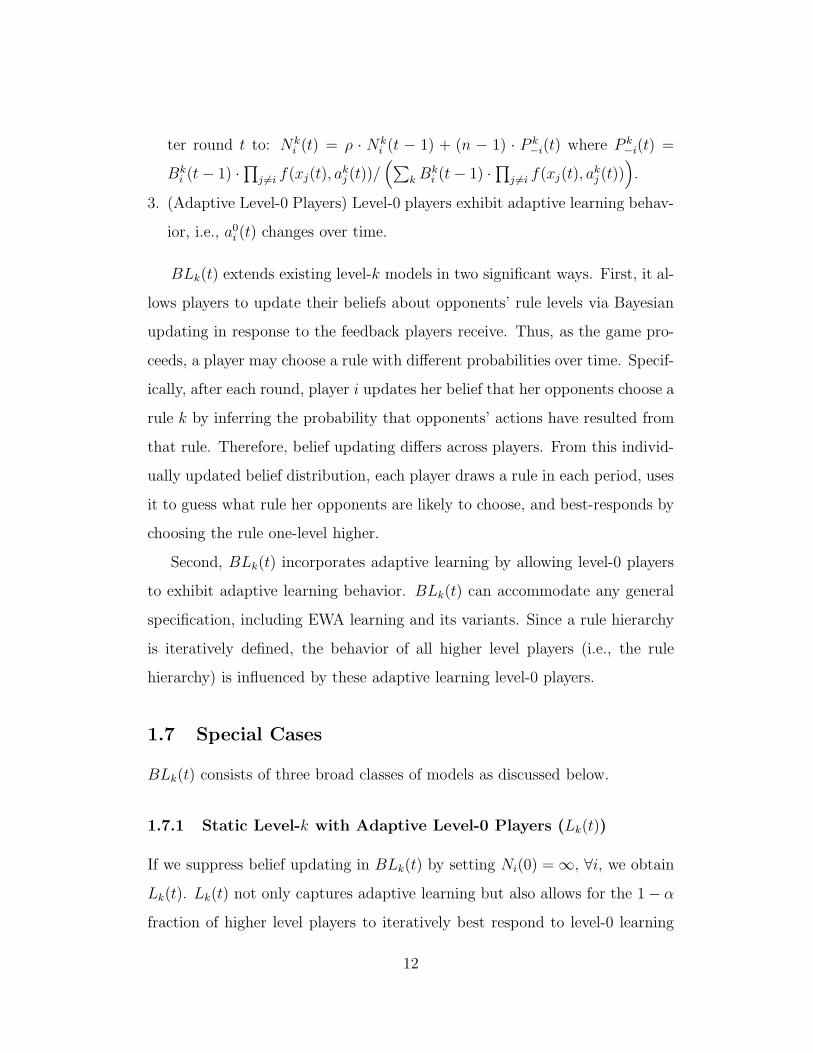
ter round t to: Nki (t) = ρ · Nk

i (t − 1) + (n − 1) · P k−i(t) where P k

−i(t) =

Bki (t− 1) ·

∏

j 6=i f(xj(t), akj (t))/

(

∑

k Bki (t− 1) ·

∏

j 6=i f(xj(t), akj (t))

)

.

3. (Adaptive Level-0 Players) Level-0 players exhibit adaptive learning behav-

ior, i.e., a0i (t) changes over time.

BLk(t) extends existing level-k models in two significant ways. First, it al-

lows players to update their beliefs about opponents’ rule levels via Bayesian

updating in response to the feedback players receive. Thus, as the game pro-

ceeds, a player may choose a rule with different probabilities over time. Specif-

ically, after each round, player i updates her belief that her opponents choose a

rule k by inferring the probability that opponents’ actions have resulted from

that rule. Therefore, belief updating differs across players. From this individ-

ually updated belief distribution, each player draws a rule in each period, uses

it to guess what rule her opponents are likely to choose, and best-responds by

choosing the rule one-level higher.

Second, BLk(t) incorporates adaptive learning by allowing level-0 players

to exhibit adaptive learning behavior. BLk(t) can accommodate any general

specification, including EWA learning and its variants. Since a rule hierarchy

is iteratively defined, the behavior of all higher level players (i.e., the rule

hierarchy) is influenced by these adaptive learning level-0 players.

1.7 Special Cases

BLk(t) consists of three broad classes of models as discussed below.

1.7.1 Static Level-k with Adaptive Level-0 Players (Lk(t))

If we suppress belief updating in BLk(t) by setting Ni(0) = ∞, ∀i, we obtain

Lk(t). Lk(t) not only captures adaptive learning but also allows for the 1− α

fraction of higher level players to iteratively best respond to level-0 learning

12

dynamics. However, Lk(t) will predict a different learning path than that of

BLk(t) because the former fails to capture sophisticated learning.

Ho et al. (1998) propose such a model with adaptive level-0 players for p-

beauty contests. In their model, rule 0 adapts over time, inducing an adaptive

rule hierarchy, whereas higher level thinkers do not adjust their rule levels. In

this regard, their model is a special case of BLk(t) with Ni(0) = ∞, ∀i.

By restricting α = 1, Lk(t) reduces to a broad class of adaptive learn-

ing models such as EWA learning and imitation learning. The EWA learning

model (Camerer and Ho, 1999; Ho et al., 2007) unifies two separate classes

of adaptive learning models: 1) reinforcement learning and 2) belief learning

models (including weighted fictitious play and Cournot best-response dynam-

ics). The weighted fictitious play model has been used to explain learning be-

havior in various games (Ellison and Fudenberg, 2000; Fudenberg and Kreps,

1993; Fudenberg and Levine, 1993). As a consequence, BLk(t) should describe

learning in these games at least equally well.

Lk(t) can also capture imitation learning models, which borrow ideas from

evolutionary dynamics. Specifically, players are assumed to mimic winning

strategies from previous rounds. These models have been applied to two- and

three-player Cournot quantity games, in which varying information is given to

players (Huck, Normann, and Oechssler, 1999; Bosch-Domenech and Vriend,

2003). Imitation learning has been shown to work well in the low information

learning environment.

Note that adaptive learning models do not allow for higher level thinkers,

who perform iterative best responses to level-0 learning dynamics. As a result,

Lk(t) is more general than the class of adaptive learning models.

13

1.7.2 Bayesian Level-k with Stationary Level-0 Players (BLk)

By setting a0i (t) = a0i (1), ∀i, t, BLk(t) reduces to BLk. In BLk, players up-

date their beliefs and sophisticatedly learn about opponents’ rule levels, while

keeping level-0 choices fixed over time. As a result, this class of models only

captures sophisticated learning. Ho and Su (2012) adopt this approach and

generalize the standard level-k model to allow players to dynamically adjust

their rule levels. Their model is shown to explain dynamic behavior in cen-

tipede and sequential bargaining games quite well. Nonetheless, their model

assumes that the strategy space and rue hierarchy of a player are equivalent.

BLk addresses this drawback by relaxing this equivalence assumption and

hence is applicable to any n-person games.

1.7.3 Static Level-k Models (Lk)

If a0i (t) = a0i (1) and Bi(t) = Bi(0), ∀i, t, then BLk(t) reduces to Lk, where

both the level-0’s choices and higher level thinkers’ beliefs are fixed over time.

Lk nests the standard level-k model as a special case, which has been used to

explain nonequilibrium behavior in applications such as auctions (Crawford

and Iriberri, 2007b), matrix games (Costa-Gomes et al., 2001), and signaling

games (Brown et al., 2012). As a result, our model will naturally capture the

empirical regularities in the above games.

There is an important difference between Lk and the standard level-k model

in the existing literature. The standard level-k model prescribes that each

player is endowed with a rule at the beginning of the game and the player

always plays that rule throughout the game. Thus, any choice of a player that

does not correspond to her prescribed rule is attributed to errors. On the other

hand, our Lk model prescribes that each player is endowed with a static belief

distribution and she makes an i.i.d draw in each round from this distribution.

14

This implies that a player may draw different rules over time even though the

belief distribution is static. As a consequence, a player’s choice dynamics over

time are interpreted as heterogeneity in i.i.d draws and hence as rational best

responses, instead of errors in her choices. Note that if each player i’s initial

prior is restricted to a point mass, Lk becomes the standard level-k model.

Note that Lk further reduces to the iterative dominance solution in dominance-

solvable games if we restrict α = 0, B∞i (0) = 1 and Bk

i (0) = 0, ∀k < ∞, ∀i

(i.e., all players have a unit mass of belief on rule ∞, which corresponds to

the iterative dominance solution). Since BLk(t) nests the iterative dominance

solution as a special case, we can use our model to evaluate the iterative dom-

inance solution empirically. Moreover, as the next proposition shows, BLk(t)

converges to the iterative dominance solution if rule 0 converges to it or if

all players are higher level thinkers whose learning dynamics satisfy a set of

conditions. (See online Appendix for the proof.)

Proposition 1. Let x∗i be player i’s unique iterative dominance solution in a

dominance-solvable game. Then, limt→∞ E [xi(t)] → x∗i , ∀i, if: (1) limt→∞ a0i (t)

→ x∗i , ∀i, or (2) limt→∞ a0i (t) 6→ x∗

i ∃ i and the following conditions (a)-(d)

are met: (a) α = 0; (b) ∀i, ρ < 1 and Ni(0) < ∞; (c) ∀i, Bi(0) follows

a uniform distribution; (d) ∀i, t, f(·, µ) > 0, infk,k′f(aki (t),a

ki (t))

f(aki (t),ak′i (t))

> 1, ∀k, k′,

supk,k′f(aki (t),a

ki (t))

f(aki (t),ak′i (t))

< ∞, ∀k, k′, and f(aki (t), ak1i (t)) = f(aki (t), a

k2i (t)) for all

mutually distinct k, k1 and k2.

2 Empirical Results

In this section, we estimate the Bayesian level-k model and its special cases

using the two games described above: p-beauty contest and generalized price

matching. Below, we describe our data, estimation methods, likelihood func-

tion, estimated models and estimation results.

15

2.1 Data

2.1.1 p-Beauty Contest

We use data from p-beauty contest games collected by Ho et al. (1998). The

experiment consisted of a 2 × 2 factorial design, where p = 0.7 or 0.9 and

n = 3 or 7. Players chose any number from [0, 100]. The prize in each round

was $1.5 for groups of size 3 and $3.5 for groups of size 7, keeping the average

prize at $0.5 per player per round. A total of 277 subjects participated in

the experiment. Each subject played the same game for 10 rounds in a fixed

matching protocol.10 For p = 0.7, there were 14 groups of size 7 and 14 groups

of size 3; for p = 0.9, there were 14 groups of size 7 and 13 groups of size 3.

Thus, we have a total of 55 groups and 2770 observations.

2.1.2 Generalized Price Matching

Before describing the generalized price matching game, we first provide our

rationale for generalizing the standard price matching game. In the standard

price matching game, the player choosing the lowest price is rewarded with a

strictly positive customer goodwill, and thus the best response is to undercut

the lowest-priced opponent by the smallest amount feasible in the strategy

space, say ǫ = $0.01. This strategic interaction is operationalized by traveler’s

dilemma described in the introduction (with ǫ = $1). As a consequence, the

rule hierarchy is defined in terms of steps of size ǫ and hence is independent of

other game parameters such as the size of the reward. Therefore, we develop a

generalized price matching game, where a rule hierarchy varies with the game

parameters. In this way, we can accommodate changes in the rule hierarchy

that may affect choice dynamics.

10Reputation building is unlikely because the p-beauty contest game is a constant-sumgame where players’ interests are strictly opposed.

16

In the generalized price matching game, n firms (players) engage in price

competition in order to attract customers. They simultaneously choose prices

in [L, U ] for a homogenous good. Firms are indexed by i (i = 1, 2, . . . , n).

Firm i’s choice of price at time t is denoted by xi(t). Let the choice vector

of all firms excluding firm i be x−i(t) = (x1(t), . . . , xi−1(t), xi+1(t), . . . , xn(t))

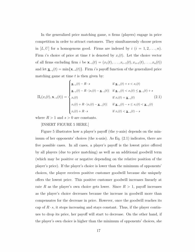
and let x−i(t) = min{x−i(t)}. Firm i’s payoff function of the generalized price

matching game at time t is then given by:

Πi(xi(t),x−i(t)) =

x−i(t)−R · s if x

−i(t) + s < xi(t)

x−i(t)−R · |xi(t)− x

−i(t)| if x−i(t) < xi(t) ≤ x

−i(t) + s

xi(t) if xi(t) = x−i(t)

xi(t) +R · |xi(t)− x−i(t)| if x

−i(t)− s ≤ xi(t) < x

−i(t)

xi(t) +R · s if xi(t) < x−i(t)− s

(2.1)

where R > 1 and s > 0 are constants.

[INSERT FIGURE 5 HERE.]

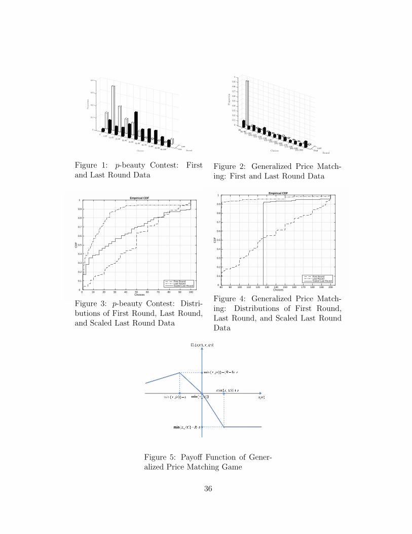
Figure 5 illustrates how a player’s payoff (the y-axis) depends on the min-

imum of her opponents’ choices (the x-axis). As Eq. (2.1) indicates, there are

five possible cases. In all cases, a player’s payoff is the lowest price offered

by all players (due to price matching) as well as an additional goodwill term

(which may be positive or negative depending on the relative position of the

player’s price). If the player’s choice is lower than the minimum of opponents’

choices, the player receives positive customer goodwill because she uniquely

offers the lowest price. This positive customer goodwill increases linearly at

rate R as the player’s own choice gets lower. Since R > 1, payoff increases

as the player’s choice decreases because the increase in goodwill more than

compensates for the decrease in price. However, once the goodwill reaches its

cap of R · s, it stops increasing and stays constant. Thus, if the player contin-

ues to drop its price, her payoff will start to decrease. On the other hand, if

the player’s own choice is higher than the minimum of opponents’ choices, she

17

receives negative customer goodwill because her price is not the lowest. The

magnitude of negative customer goodwill increases linearly in the player’s own

choice. However, once the goodwill reaches its cap of −R · s, its magnitude

stops increasing and stays constant. If the player’s own choice and the mini-

mum of her opponents’ choices are identical, she receives neither positive nor

negative customer goodwill and the payoff is simply the lowest price.

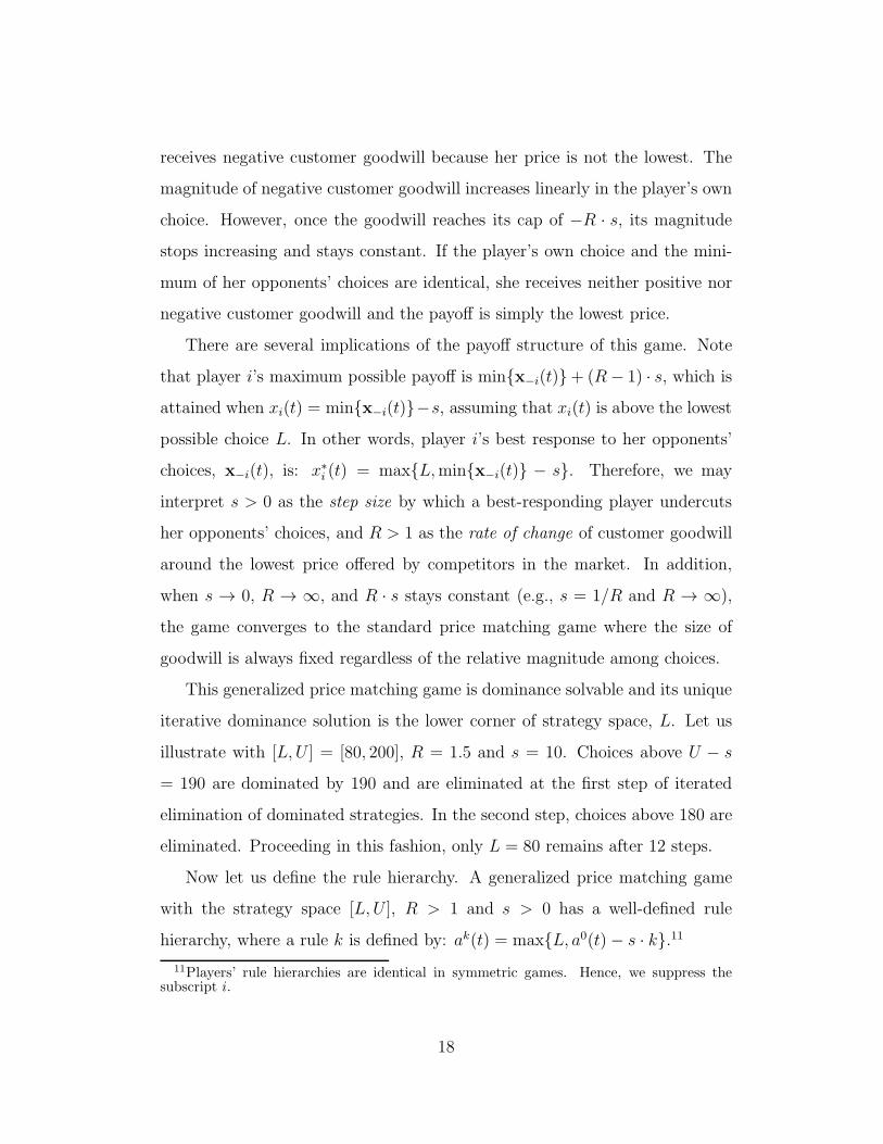
There are several implications of the payoff structure of this game. Note

that player i’s maximum possible payoff is min{x−i(t)}+ (R− 1) · s, which is

attained when xi(t) = min{x−i(t)}−s, assuming that xi(t) is above the lowest

possible choice L. In other words, player i’s best response to her opponents’

choices, x−i(t), is: x∗i (t) = max{L,min{x−i(t)} − s}. Therefore, we may

interpret s > 0 as the step size by which a best-responding player undercuts

her opponents’ choices, and R > 1 as the rate of change of customer goodwill

around the lowest price offered by competitors in the market. In addition,

when s → 0, R → ∞, and R · s stays constant (e.g., s = 1/R and R → ∞),

the game converges to the standard price matching game where the size of

goodwill is always fixed regardless of the relative magnitude among choices.

This generalized price matching game is dominance solvable and its unique

iterative dominance solution is the lower corner of strategy space, L. Let us

illustrate with [L, U ] = [80, 200], R = 1.5 and s = 10. Choices above U − s

= 190 are dominated by 190 and are eliminated at the first step of iterated

elimination of dominated strategies. In the second step, choices above 180 are

eliminated. Proceeding in this fashion, only L = 80 remains after 12 steps.

Now let us define the rule hierarchy. A generalized price matching game

with the strategy space [L, U ], R > 1 and s > 0 has a well-defined rule

hierarchy, where a rule k is defined by: ak(t) = max{L, a0(t)− s · k}.11

11Players’ rule hierarchies are identical in symmetric games. Hence, we suppress thesubscript i.

18

Since the generalized price matching game had not been studied previously,

we conducted a new experiment to collect data. The experiment consisted of

a 2x2 factorial design with n = (3, 7) and s = (5, 10). We set R = 1.5 for

all experimental conditions. A total of 157 students from a major university

in Southeast Asia participated in the experiment, with 7 groups in the exper-

imental condition of n = 3 and s = 10, and 8 groups in each of the three

remaining experimental conditions. Subjects chose any number from [80, 200].

Each subject played the same game for 10 rounds in a random matching pro-

tocol.12 In each round, subjects accumulated points according to the payoff

function in Eq. (2.1). After all 10 rounds, these points were converted to dol-

lars at a rate of $0.01 per point. The equilibrium payoff in all experimental

conditions was fixed at $8. In addition, all participants were paid a $5 show-up

fee.13 The full set of instructions is given in the online Appendix.

2.2 Estimation Methods

In empirical estimation, we normalized the data as in Ho et al. (1998) so

that each round’s data has equal influence on the estimation.14 Since both

games are symmetric, we assumed a common prior belief distribution among

the players, i.e., B(0) = Bi(0), ∀i and N(0) = Ni(0), ∀i.15

We assumed that the probability density function f(x, µ) in Eq. (1.1)

follows a normal distribution with mean µ and standard deviation σ, i.e.,

12We used a random matching protocol to avoid reputation building since the pricematching game has outcomes that are Pareto-superior to the equilibrium outcome. Datashows convergence towards equilibrium, which means that reputation building was indeedthwarted. However, 9.8% of all choices were 200, suggesting that some players still triedreputation building albeit unsuccessfully. We excluded these choices in the estimation.

13The prevailing exchange rate at the time of the experiment was US$1 = $1.20.14Generally, variance drops over time as convergence takes place. As a result, if data is

not normalized, later rounds’ data will have more influence on the estimation. Specifically,

xi(t) and aki(t)i

(t) were normalized to (xi(t) − µ(t))/s(t) and (aki(t)i

(t) − µ(t))/s(t) whereµ(t) and s(t) are the sample mean and sample standard deviation at time t, respectively.

15In the belief updating process, as in Camerer and Ho (1999), we restrictN(0) ≤ 1/(1−ρ)so that the belief updating obeys the law of diminishing effect. That is, the incrementaleffect of later observations diminishes as learning equilibrates.

19

f(x, µ) = N (x, µ, σ) where N (x, µ, σ) denotes the normal density with mean µ

and standard deviation σ evaluated at x.16 The standard deviation σ was

empirically estimated. We also estimated a separate standard deviation, σ0,

for the choices of level-0 players, in order to investigate whether these non-

sophisticated thinkers’ choices are more noisy.17

Next, we assumed a common level-0 behavior across players since the game

is symmetric, i.e., a0i (t) = a0(t), ∀i. Further, we assumed that level-0 players

are imitation learners who mimic past periods’ winning actions that yielded

the highest payoff, i.e., a0(t) follows imitation learning dynamics. Specifically,

let ω(t) be the winning action with the highest payoff in time t that is actually

chosen by one or more players, and let ω(0) be the a priori winning strategy

before the game starts. Then, the rule 0 at time t corresponds to a weighted

sum of the rule 0’s choice at time t− 1 and the most recent winning action at

time t− 1. Formally, a0(t) is defined by:

a0(1) = ω(0)

a0(t) = δ · a0(t− 1) + (1− δ) · ω(t− 1) (t ≥ 2)

where δ is the weight given to the rule 0’s choice in the previous round. Thus,

δ captures the rate at which a player decays past winning actions. Note that

when δ = 0, level-0 players completely decay history after each round and

simply repeat the most recent winning strategy. Hence, a level-1 thinker who

best-responds to this captures Cournot best-response dynamics. On the other

hand, when δ = 1, level-0 players never incorporate observed game plays and

their choices remain unchanged, i.e., a0(t) = a0(1) = ω(0), ∀t.18

16Subjects’ actual choices were always discrete; in p-beauty contest games, choices werealways integers and in generalized pricing matching games, choices never had more thanone decimal point. Therefore, we discretized the strategy space, f(x, µ) and the likelihoodfunction given below into intervals of 1 for the prior and 0.1 for the latter in our estimation.

17Since we used normalized data, N (x, µ, σ0) and N (x, µ, σ) become close to the uniformdistribution for σ0 and σ big enough across both games. Thus, we bounded σ0 and σ fromabove by 20 in the estimation. Estimation results were not sensitive to increasing the bound.

18We also fit the models with a0(t) specified as the weighted fictitious play (Fudenberg

20

We devoted the first round data entirely to calibrating parameter estimates

for the a priori winning strategy at time 0, ω(0), and the prior belief distri-

bution, B(0).19 Calibrating the first round data serves two purposes. First, it

helps control for the initial heterogeneity in belief draws before any learning

takes place. Second, it mitigates under- or over-estimating the speed of learn-

ing. For instance, choices too far from the equilibrium may be misattributed to

slow adaptive learning by level-0 players, i.e., the model may wrongly predict

slow convergence of a0(t) towards the equilibrium in order to explain those

choices. Moreover, in extremely fast converging games, the prior belief distri-

bution may be estimated to be skewed towards higher rule levels in order to

explain the high proportion of equilibrium choices overall. This may result in

underestimating the speed of belief updating, i.e., overestimating the stickiness

parameter N(0) or the memory decay factor ρ in belief updating.

We used the maximum likelihood estimation method with the MATLAB

optimization toolbox. To ensure that the maximized likelihood is indeed the

global maximum, we utilized multiple starting points in the optimization rou-

tine.20 The 95 % confidence intervals of parameter estimates were empirically

constructed using the jackknife method. These confidence intervals are re-

ported in parentheses below parameter estimates in Tables 1 and 2.

and Levine, 1998). The weighted fictitious play fits poorly. The results are available uponrequest from the authors.

19Without imposing any parametric assumptions on the belief distribution, we used asmany free parameters as the rules that fit in the strategy space. Let this number of rulesbe K. Note that K = ∞ in our p-beauty contest games since rule ∞ corresponds to theequilibrium. Hence, in the estimation, we instead used K large enough (K = 50) and theestimation results were not sensitive to having a higher number of rules.We used the maximum likelihood estimation method. For notational consistency, let us

treat the first round data as data at time 0, i.e., {xi(0) | ∀i} refers to the first round dataused for calibration purposes only. Then, the log-likelihood of observing the first round data

is given by:∑

ilog

(

∑

K

k=0 Bk(0) · N (xi(0), a

k(0), σ))

where a0(0) = ω(0) and ak(0) (k ≥ 1)

is defined iteratively. Here, σ is the error term used only for the first round estimation. Theestimated ω(0), B(0) and ˆσ are described in footnotes in Tables 1 and 2.

20We randomly selected 20 starting points in the parametric space.

21

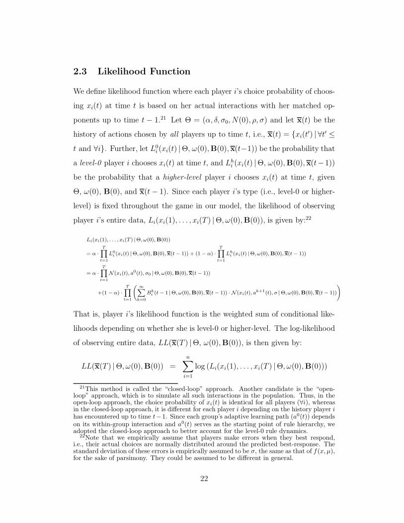
2.3 Likelihood Function

We define likelihood function where each player i’s choice probability of choos-

ing xi(t) at time t is based on her actual interactions with her matched op-

ponents up to time t − 1.21 Let Θ = (α, δ, σ0, N(0), ρ, σ) and let x(t) be the

history of actions chosen by all players up to time t, i.e., x(t) = {xi(t′) | ∀t′ ≤

t and ∀i}. Further, let L0i (xi(t) |Θ, ω(0),B(0),x(t−1)) be the probability that

a level-0 player i chooses xi(t) at time t, and Lhi (xi(t) |Θ, ω(0),B(0),x(t−1))

be the probability that a higher-level player i chooses xi(t) at time t, given

Θ, ω(0), B(0), and x(t− 1). Since each player i’s type (i.e., level-0 or higher-

level) is fixed throughout the game in our model, the likelihood of observing

player i’s entire data, Li(xi(1), . . . , xi(T ) |Θ, ω(0),B(0)), is given by:22

Li(xi(1), . . . , xi(T ) |Θ, ω(0),B(0))

= α ·T∏

t=1

L0i (xi(t) |Θ, ω(0),B(0),x(t − 1)) + (1− α) ·

T∏

t=1

Lhi (xi(t) |Θ, ω(0),B(0), x(t − 1))

= α ·T∏

t=1

N (xi(t), a0(t), σ0 |Θ, ω(0),B(0),x(t − 1))

+(1− α) ·T∏

t=1

(

∞∑

k=0

Bki (t − 1 |Θ, ω(0),B(0),x(t − 1)) · N (xi(t), a

k+1(t), σ |Θ, ω(0),B(0),x(t− 1))

)

That is, player i’s likelihood function is the weighted sum of conditional like-

lihoods depending on whether she is level-0 or higher-level. The log-likelihood

of observing entire data, LL(x(T ) |Θ, ω(0),B(0)), is then given by:

LL(x(T ) |Θ, ω(0),B(0)) =

n∑

i=1

log (Li(xi(1), . . . , xi(T ) |Θ, ω(0),B(0)))

21This method is called the “closed-loop” approach. Another candidate is the “open-loop” approach, which is to simulate all such interactions in the population. Thus, in theopen-loop approach, the choice probability of xi(t) is identical for all players (∀i), whereasin the closed-loop approach, it is different for each player i depending on the history player ihas encountered up to time t−1. Since each group’s adaptive learning path (a0(t)) dependson its within-group interaction and a0(t) serves as the starting point of rule hierarchy, weadopted the closed-loop approach to better account for the level-0 rule dynamics.

22Note that we empirically assume that players make errors when they best respond,i.e., their actual choices are normally distributed around the predicted best-response. Thestandard deviation of these errors is empirically assumed to be σ, the same as that of f(x, µ),for the sake of parsimony. They could be assumed to be different in general.

22

Note that ω(0) and B(0) were separately estimated using the first round data.

In sum, we estimated a total of 6 parameters Θ = (α, δ, σ0, N(0), ρ, σ): for

level-0 players, we estimated the probability that a player is only a level-0,

adaptive-learning player throughout the game (α), the decaying rate of past

winning actions in imitation learning (δ) and the error term for these adaptive

level-0 players (σ0); for Bayesian belief updating, we estimated the stickiness

parameter of initial priors (N(0)), memory decay factor (ρ) and the error term

for the sophisticated, belief-updating players (σ).

2.4 Estimated Models

We estimated a total of 4 models, which can be classified into two groups.

The first group includes 2 models that incorporate adaptive level-0 players

(i.e., a0(t)) while the second group includes 2 models that do not incorporate

adaptive level-0 players (i.e., a0(t) = a0(1), ∀t). The full model BLk(t) nests

the other 3 models as special cases. By comparing the fit of our model with that

of nested cases, we can determine the importance of adaptive and sophisticated

learning. The first group includes the following 2 models:

1. Bayesian level-k model with adaptive level-0 (BLk(t)): This is the full

model with the parametric space (α, δ, σ0, N(0), ρ, σ) having 6 parameters.

The first three parameters capture level-0’s adaptive learning while the last

three parameters capture higher level thinkers’ sophisticated learning.

2. Static level-k model with adaptive level-0 (Lk(t)): This model allows level-

0 players to adaptively learn and a0(t) to change over time. However, the

rule levels of higher level thinkers remain fixed over time. This model is

a nested case of BLk(t) with N(0) = ∞ and ρ = 1, i.e., the parametric

space is (α, δ, σ0,∞, 1, σ). If we further restrict α = 1, Lk(t) reduces to

pure adaptive learning models which include experience-weighted attraction

23

learning, fictitious play (Brown, 1951), and reinforcement learning models.

The second group includes the following 2 models:

3. Bayesian level-k model with stationary level-0 (BLk): This model ignores

level-0’s adaptive learning and only captures sophisticated learning. Specif-

ically, it allows higher level thinkers to update their beliefs after each round

about what rules others are likely to choose. As a result, these higher level

thinkers choose a rule with different probabilities over time. This model is

obtained by setting δ = 1 in BLk(t), i.e., a0(t) = a0(1), ∀t. The resulting

parametric space is (α, 1, σ0, N(0), ρ, σ).

4. Static level-k with stationary level-0 (Lk): This captures neither adaptive

learning nor sophisticated learning. It is obtained by setting N(0) = ∞

and ρ = δ = 1. The resulting parametric space is (α, 1, σ0,∞, 1, σ).

2.5 Estimation Results

Tables 1 and 2 show the estimation results. In both tables, the first column lists

the names of parameters and test statistics. The 4 columns to the right of that

report results from each of the four estimated models. The top panel reports

parameter estimates and the bottom panel reports maximized log-likelihood

and test statistics. We report χ2, Akaike Information Criterion (AIC) and

Bayesian Information Criterion (BIC).

The bottom panels show that BLk(t) fits the data best. All three nested

cases are strongly rejected in favor of BLk(t). This is true regardless of which

test statistic is used. Below we discuss the estimation results in detail.

2.5.1 p-beauty Contest Games

The bottom panel of Table 1 shows that BLk(t) fits the data much better

than the three special cases. In fact, all three test statistics (χ2, AIC, and

24

BIC) indicate that the three special cases are strongly rejected in favor of

BLk(t). For instance, the χ2 test statistics of Lk, BLk, and Lk(t) against

BLk(t) are 3082.15, 744.52, and 336.58, respectively. These results suggest

that allowing Bayesian updating by higher level thinkers and having adaptive

level-0 players are both crucial in explaining subjects’ dynamic choices over

time. Put differently, higher level thinkers not only are aware that level-0

players adapt their choices, but also adjust their rule levels over time.23

[INSERT TABLE 1 HERE.]

The estimated parameters of BLk(t) appear reasonable. The fraction of

adaptive level-0 players (α) is estimated to be 38%. These adaptive level-0

players assign equal weight to the most recent observed winning action and

their own past choices (i.e., δ = 50%), suggesting that players notice that

the winning actions are converging towards equilibrium. The level-0 players’

choices have a standard deviation of σ0 = 1.68, and their choices are more

variable than those of higher level thinkers (σ = 0.32).24

The parameter estimates of higher level thinkers (k ≥ 1) are also sensible.

These higher level thinkers give their initial priors the weight N(0) = 3.35 and

decay this prior weight at a rate of ρ = 0.4. That is, the influence of the initial

prior drops to 3.35 · 0.4t after t rounds. Note that the standard deviation of

level-k thinkers is estimated to be σ = 0.32, implying that their choices are

significantly less noisy than those of level-0 players.

We note the following patterns in other parameter estimates:

1. Comparing the left and right panels of Table 1, we observe that the choices

of level-0 players become significantly less variable if they are allowed to

23We also fit a model of pure adaptive learning by setting α = 1 (i.e., all players areadaptive level-0 players who engage in imitation learning). The estimated model has amaximized log-likelihood of -10341 and is strongly rejected in favor of BLk(t) with χ2 =1298.

24In the estimation, we normalized subjects’ choices by the sample standard deviation.As a consequence, a σ value of 1 means that choices are as variable as those made by anaverage player in the population.

25

adapt (σ0 drops from 19.990 to 1.565).

2. Allowing for either adaptive level-0 players or Bayesian updating of rule

levels by higher level thinkers makes the latter players’ choices less variable

(σ drops from 1.10 to 0.320).

3. On the right panel of the table, we see that the fraction of level-0 players

drops from 48% to 38%. This means that if we did not allow players to

change their rule levels, the fraction of higher level thinkers would be under-

estimated.

4. Across the four models, allowing higher level thinkers to update their beliefs

reduces the weight placed on the history (ρ drops from 1 to 0.345).

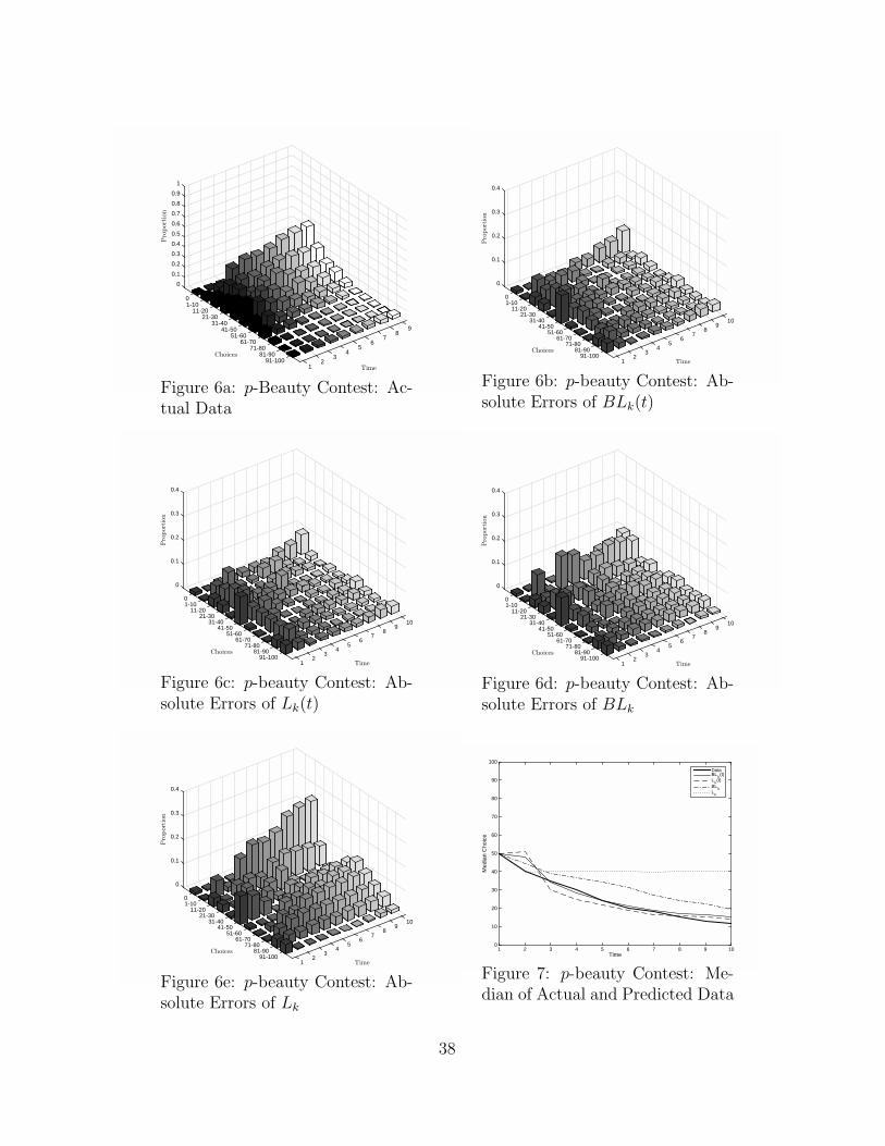
Figure 6a presents three-dimensional bar graphs of actual choice frequency

of experimental data. Figures 6b-6e show the absolute errors (= |Predicted

Choice Frequency − Actual Choice Frequency|) over time for the four models.

In these absolute error plots, a perfect model will generate a bar graph of zero

frequency in every choice bracket in every round. The poorer a model is, the

higher its bar graph will be. Figure 7 shows median choices from actual data

as well as those predicted by the four models.25 Note the following:

1. We start with the simplest static level-k model, Lk. As shown in Figure 6e,

this model fits the data poorly. In fact, its absolute error increases over

time. Figure 7 confirms this and shows that Lk consistently over-predicts

median choices from round 3 onward. This result is not surprising given

that Lk ignores both adaptive and sophisticated learning. In this regard,

our model represents a significant extension of Lk in terms of both theory

and empirical fit.

25Note that both the actual and predicted data distributions become skewed towards theequilibrium as convergence takes place and as a result, their average choices become sensitiveto off-equilibrium choices over time. Thus, we used the median instead of average choice formodel comparisons.

26

2. Model BLk allows higher-level thinkers to learn while keeping level-0 players

fixed over time. As shown in Figure 6d, this model fits the data better than

Lk, suggesting that sophisticated learning helps to capture choice dynamics.

Figure 7 shows that after round 3, BLk’s predicted median choice is con-

sistently closer to the actual median choice than Lk’s. However, BLk still

consistently over-predicts actual choices (i.e., its median is always higher

than the actual median).

3. Model Lk(t) incorporates adaptive level-0 players by allowing them to im-

itate past winners. However, higher level thinkers are assumed to hold

stationary beliefs about their opponents’ rule levels. Figure 6c shows a

significant reduction in bar heights compared to Figures 6d and 6e, sug-

gesting that Lk(t) yields predictions closer to actual data than BLk and

Lk. Figure 7 shows that Lk(t) fits the data better than the other two

nested models by significantly reducing the gap between predicted and ac-

tual median choices, starting in round 4. These patterns are also consistent

with the result in Table 1 that Lk(t) is the second best-fitting model.

4. Model BLk(t) allows for both adaptive level-0 players and higher level

thinkers’ sophisticated learning. Not surprisingly, Figure 6b shows that

BLk(t) produces the lowest error bars among the four models. Compared

to Lk(t), the superiority of BLk(t) occurs in the earlier rounds (rounds 2

to 5). This suggests that adaptive learning alone fails to adequately cap-

ture actual choice dynamics in early rounds and that sophisticated learning

helps close this gap. This superiority in earlier rounds is also demonstrated

in Figure 7 where BLk(t) tracks the actual median choice better than Lk(t)

up to round 7, during which significant convergence to equilibrium occurs.

[INSERT FIGURE 6a-6e and 7 HERE.]

27

2.5.2 Generalized Price Matching Games

The bottom panel of Table 2 shows that BLk(t) fits the data best. All three

test statistics (χ2, AIC, and BIC) suggest that the three nested models are

strongly rejected in favor of the BLk(t). For instance, the BIC test statistics

were 14481.81, 12982.87, 12859.85 and 12699.05 for Lk, BLk, Lk(t) and BLk(t),

respectively, in favor of BLk(t). These results suggest that both types of

learning are pivotal in explaining choice dynamics in data.26

[INSERT TABLE 2 HERE.]

The estimated fraction of adaptive level-0 players (α) is 26%. These adap-

tive level-0 players assign a weight of δ = 66% to the past level-0’s choice.

As before, the choices of level-0 players also have a higher standard deviation

than those of higher level thinkers (σ0 = 2.21 versus σ = 0.03).

Three quarters of the subjects are higher level thinkers. These players give

their initial priors the weight N(0) = 10.23 and decay this prior weight at a

rate of ρ = 0.80 after each round. That is, the influence of initial prior drops

to 10.23 · 0.80t after t rounds.

Note the following on the parameter estimates reported in Table 2:

1. Comparing the left and right panels of Table 1, we see that level-0 players’

choices become significantly less variable if they are allowed to adapt (σ0

drops from 19.990 to 1.985).

2. Allowing for either adaptive level-0 players or Bayesian belief updating

introduces some variability into higher level thinkers’ choices (σ increases

from 0.00 to 0.027).

3. The right panel of the table shows that the fraction of level-0 players drops

from 33% to 26%. This means if we did not allow higher level thinkers to so-

26We also fit a model of pure adaptive learning by setting α = 1 (i.e., all players areadaptive, imitation learners). The estimated model has a maximized log-likelihood -6987.49and is rejected in favor of BLk(t) with χ2 = 1319.

28

phisticatedly learn, the fraction of these players would be under-estimated.

4. Allowing higher level thinkers to update their beliefs reduces the weight

placed on the history (ρ drops from 1 to 0.745).

In sum, these parameter estimates are remarkably similar to those from the

p-beauty contest games. This is surprising, but encouraging, given that the

two games are different and that subjects’ choices converge towards equilibrium

much faster in generalized price matching games.

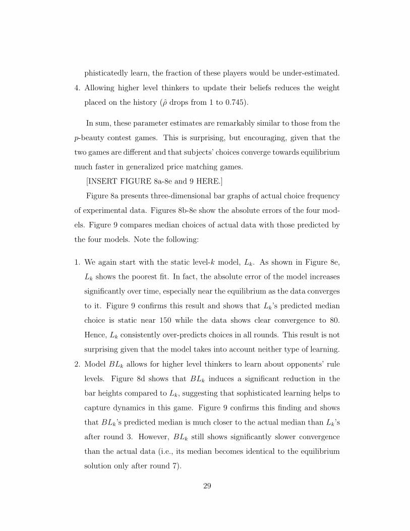
[INSERT FIGURE 8a-8e and 9 HERE.]

Figure 8a presents three-dimensional bar graphs of actual choice frequency

of experimental data. Figures 8b-8e show the absolute errors of the four mod-

els. Figure 9 compares median choices of actual data with those predicted by

the four models. Note the following:

1. We again start with the static level-k model, Lk. As shown in Figure 8e,

Lk shows the poorest fit. In fact, the absolute error of the model increases

significantly over time, especially near the equilibrium as the data converges

to it. Figure 9 confirms this result and shows that Lk’s predicted median

choice is static near 150 while the data shows clear convergence to 80.

Hence, Lk consistently over-predicts choices in all rounds. This result is not

surprising given that the model takes into account neither type of learning.

2. Model BLk allows for higher level thinkers to learn about opponents’ rule

levels. Figure 8d shows that BLk induces a significant reduction in the

bar heights compared to Lk, suggesting that sophisticated learning helps to

capture dynamics in this game. Figure 9 confirms this finding and shows

that BLk’s predicted median is much closer to the actual median than Lk’s

after round 3. However, BLk still shows significantly slower convergence

than the actual data (i.e., its median becomes identical to the equilibrium

solution only after round 7).

29

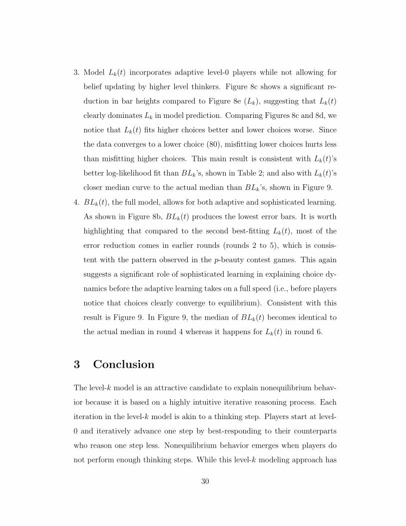
3. Model Lk(t) incorporates adaptive level-0 players while not allowing for

belief updating by higher level thinkers. Figure 8c shows a significant re-

duction in bar heights compared to Figure 8e (Lk), suggesting that Lk(t)

clearly dominates Lk in model prediction. Comparing Figures 8c and 8d, we

notice that Lk(t) fits higher choices better and lower choices worse. Since

the data converges to a lower choice (80), misfitting lower choices hurts less

than misfitting higher choices. This main result is consistent with Lk(t)’s

better log-likelihood fit than BLk’s, shown in Table 2; and also with Lk(t)’s

closer median curve to the actual median than BLk’s, shown in Figure 9.

4. BLk(t), the full model, allows for both adaptive and sophisticated learning.

As shown in Figure 8b, BLk(t) produces the lowest error bars. It is worth

highlighting that compared to the second best-fitting Lk(t), most of the

error reduction comes in earlier rounds (rounds 2 to 5), which is consis-

tent with the pattern observed in the p-beauty contest games. This again

suggests a significant role of sophisticated learning in explaining choice dy-

namics before the adaptive learning takes on a full speed (i.e., before players

notice that choices clearly converge to equilibrium). Consistent with this

result is Figure 9. In Figure 9, the median of BLk(t) becomes identical to

the actual median in round 4 whereas it happens for Lk(t) in round 6.

3 Conclusion

The level-k model is an attractive candidate to explain nonequilibrium behav-

ior because it is based on a highly intuitive iterative reasoning process. Each

iteration in the level-k model is akin to a thinking step. Players start at level-

0 and iteratively advance one step by best-responding to their counterparts

who reason one step less. Nonequilibrium behavior emerges when players do

not perform enough thinking steps. While this level-k modeling approach has

30

been successfully applied to both laboratory and field experiments, it is far

from complete since the level-k model is inherently static. A wide body of

empirical evidence shows that behavior converges to equilibrium over time.

To capture such dynamic choice behavior, this paper proposes a Bayesian

level-k model that distinguishes between two possible types of learning dynam-

ics. One possibility is that the starting point of the iterative reasoning process

(i.e., level-0) moves towards equilibrium, so players approach the equilibrium

while performing the same number of thinking steps throughout. Another pos-

sibility is that players approach the equilibrium by engaging in more thinking

steps. In sum, our model generalizes the standard level-k model in two signif-

icant ways:

1. We allow the level-0 rule to adaptively respond to historical game plays (e.g.,

past winning or chosen actions). To the extent that observed game plays

move towards equilibrium, players may approach the equilibrium without

advancing in rule levels. In this way, players exhibit adaptive learning.

2. We allow players to revise their rule levels by Bayesian updating, where

players update beliefs about opponents’ rule levels based on observations.

Thus, players perform more thinking steps when they anticipate likewise

from opponents. In this way, players exhibit sophisticated learning.

Interestingly, the extended model provides a novel unification of two sepa-

rate streams of nonequilibrium models: level-k and adaptive learning models.

On one hand, level-k models are “static” and have been used to predict behav-

ior in one-shot games. On the other hand, adaptive learning models have been

used to describe choice dynamics in repeated games. While these two seem-

ingly distinct classes of models have been treated separately in the literature,

our model brings them together and provides a sensible way to model behavior

in both one-shot and repeated games in a common, tractable framework.

31

We apply the Bayesian level-k model to experimental data on two games: p-

beauty contest (from Ho et al. (1998)) and generalized price matching (freshly

collected through new experiments). For both games, we find strong evidence

that our model explains the data better than all its special cases and that it is

essential to account for sophisticated learning even after existing nonequilib-

rium models are introduced. In other words, beyond merely best responding

to historical game plays, players dynamically adjust their rule levels over time

in response to changing anticipation about opponents’ rule levels.

By incorporating both adaptive and sophisticated learning, our model can

be viewed as a characterization of the equilibration process. This view bears

the same spirit as Harsanyi’s “tracing procedure” (Harsanyi and Selten, 1988),

in which players’ successive choices, as they react to new information in strate-

gic environments, trace a path towards the eventual equilibrium outcome.

References

Basu, K. 1994. “The Traveler’s Dilemma: Paradoxes of Rationality in Game

Theory.” Am. Econ. Rev. 84(2): 391-395.

Binmore, K., A. Shaked and J. Sutton. 1985. “Testing Noncooperative Bar-

gaining Theory: A Preliminary Study.” Am. Econ. Rev. 75: 1178-1180.

Bosch-Domenech, A., J. G. Montalvo, R. Nagel and A. Satorra. 2002. “One,

Two, (Three), Infinity, ... : Newspaper and Lab Beauty-Contest Experi-

ments.” Am. Econ. Rev. 92(5): 1687-1701.

Bosch-Doenech, A. and N. J. Vriend. 2003. “Imitation of successful behaviour

in the markets.” The Economic Journal 113: 495524.

Brown, A., C. F. Camerer and D. Lovallo. 2012. “To Review or Not To

Review? Limited Strategic Thinking at the Movie Box Office.” American

Economic Journal: Microeconomics 4(2): 1-28.

32

Brown, George W. 1951. “Iterative solution of games by fictitious play.” Ac-

tivity Analysis of Production and Allocation 13(1): 374-376.

Camerer, C. and T-H. Ho. 1999. “Experience-Weighted Attraction Learning

in Normal Form Games.” Econometrica 67: 837-874.

Camerer, C. F., T-H. Ho and J-K. Chong. 2004. “A Cognitive Hierarchy

Model of Games.” Quarterly Journal of Economics 119(3): 861-898.

Chen, Y., C. Narasimhan and Z. J. Zhang. 2001. “Consumer heterogeneity

and competitive price-matching guarantees.” Market Sci. 20(3): 300-314.

Capra, C. M., J. K. Goeree, R. Gomez and C. A. Holt. 1999. “Anomalous

Behavior in a Traveler’s Dilemma?.” Am. Econ. Rev. 89(3): 678-690.

Costa-Gomes, M., V. Crawford and B. Broseta. 2001. “Cognition and Be-

havior in Normal-Form Games: An Experimental Study.” Econometrica 69:

1193-1235.

Costa-Gomes, M. and V. Crawford. 2006. “Cognition and Behavior in Two-

Person Guessing Games: An Experimental Study.” Am. Econ. Rev. 96: 1737-

1768.

Costa-Gomes, M. and G. Weizsacker. 2008. “Stated Beliefs and Play in

Normal-Form Games.” Review of Economic Studies 75(3): 729-762.

Costa-Gomes, M., V. Crawford and N. Iriberri. 2009. “Comparing Models of

Strategic Thinking in Van Huyck, Battalio, and Beil’s Coordination Games.”

Journal of the European Economic Association 7: 377-387.

Crawford, V. P. 2003. “Lying for Strategic Advantage: Rational and Bound-

edly Rational Misrepresentation of Intentions.” Am. Econ. Rev. 93: 133-149.

Crawford, V. P. and N. Iriberri. 2007a. “Fatal Attraction: Salience, Naivete,

and Sophistication in Experimental Hide-and-Seek Games.” Am. Econ. Rev.

97: 1731-1750.

33

Crawford, V. P. and N. Iriberri. 2007b. “Level-k Auctions: Can a Non-

Equilibrium Model of Strategic Thinking Explain the Winner’s Curse and

Overbidding in Private-Value Auctions?.” Econometrica 75: 1721-1770.

Crawford, V. P., T. Kugler, Z. Neeman and A. Pauzner. 2009. “Behaviorally

Optimal Auction Design: An Example and Some Observations.” Journal of

the European Economic Association 7(2-3): 377-387.

Crawford, V. P., M. A. Costa-Gomes and N. Iriberri. 2013. “Structural Mod-

els of Nonequilibrium Strategic Thinking: Theory, Evidence, and Applica-

tions.” Journal of Economic Literature, In Press.

Ellison, G. and D. Fudenberg. 2000. “Learning Purified Mixed Equilibria.”

J. Econ. Theory 90(1): 84-115.

Fudenberg, D. and D. Kreps. 1993. “Learning mixed equilibria.” Games and

Economic Behavior 5: 320-367

Fudenberg, D. and D. Levine. 1993. “Steady State Learning and Nash Equi-

librium.” Econometrica 61(3): 547-573.

Fudenberg, D. and D. Levine. 1998. “Theory of Learning in Games.” Cam-

bridge, MIT Press.

Goldfarb, A. and B. Yang. 2009. “Are All Managers Created Equal?.” J.

Marketing Res. 46(5): 612-622.

Goldfarb, A. and M. Xiao. 2011. “Who Thinks About the Competition?

Managerial Ability and Strategic Entry in US Local Telephone Markets.”

Am. Econ. Rev. 101(7): 3130-3161.

Goeree, J. K. and C. A. Holt. 2001. “Ten Little Treasures of Game Theory

and Ten Intuitive Contradictions.” Am. Econ. Rev. 91(5):1402-1422.

Harsanyi, J. C. and R. Selten. 1988. “A General Theory of Equilibrium Se-

lection in Games.” Cambridge, MIT Press.

Huck, S., H. Normann and J. Oechssler. 1999. “Learning in Cournot

Oligopoly–An Experiment.” Economic Journal 109: C80-C95.

34

Ho, T-H., C. Camerer and K. Weigelt. 1998. “Iterated Dominance and It-

erated Best Response in Experimental p-Beauty Contests.” Am. Econ. Rev.

88: 947-969.

Ho, T-H., C. Camerer, C. and J-K. Chong. 2007. “Self-tuning Experience-

Weighted Attraction Learning in Games.” J. Econ. Theory 133(1): 177-198.

Ho, T-H. and X. Su. 2013. “A Dynamic Level-k Model in Sequential Games.”

Manage. Sci. 59(2): 452-469.

Jain, S. and J. Srivastava. 2000. “An experimental and theoretical analysis

of price-matching refund policies.” J. Marketing Res. 37(3): 351-362.

Nagel, R. 1995. “Unraveling in Guessing Games: A Experimental Study.”

Am. Econ. Rev. 85(5): 1313-26.

McKelvey, R. D. and T. R. Palfrey. 1992. “An Experimental Study of the

Centipede Game.” Econometrica 60: 803-836.

Ochs, J. and A. E. Roth. 1989. “An Experimental Study of Sequential Bar-

gaining.” Am. Econ. Rev. 79: 355-384.

Ostling, R., J. T-Y. Wang, E. Chou and C. Camerer. 2011. “Testing Game

Theory in the Field: Swedish LUPI Lottery Games.” American Economic

Journal: Microeconomics 3(3): 1-33.

Srivastava, J. and N. Lurie. 2001. “A Consumer Perspective on Price? Match-

ing Refund Policies: Effect on Price Perceptions and Search Behavior.” Jour-

nal of Consumer Research 28(2): 296-307.

Stahl, D. and P. Wilson. 1994. “Experimental Evidence on Players’ Models

of Other Players.” J. Econ. Behav. Organ. 25 (3): 309-327.

Stahl, D. and P. Wilson. 1995. “On Players’ Models of Other Players - Theory

and Experimental Evidence.” Games and Economic Behavior 10: 213-254.

35

Round

Last

First91-10081-90

71-8061-70

Choices

51-6041-50

31-4021-30

11-201-10

0

0.4

0.3

0.2

0.1

0

Proportion

Figure 1: p-beauty Contest: Firstand Last Round Data

Round

LastFirst191-200

181-190171-180

161-170151-160

Choices

141-150131-140

121-130111-120

101-11091-100

81-9080

1

0.9

0.8

0.7

0.6

0.5

0.4

0.3

0.2

0.1

0

Proportion

Figure 2: Generalized Price Match-ing: First and Last Round Data

Choices0 10 20 30 40 50 60 70 80 90 100

CD

F

0

0.1

0.2

0.3

0.4

0.5

0.6

0.7

0.8

0.9

1 Empirical CDF

First RoundLast RoundScaled Last Round

Figure 3: p-beauty Contest: Distri-butions of First Round, Last Round,and Scaled Last Round Data

Choices80 90 100 110 120 130 140 150 160 170 180 190 200

CD

F

0

0.1

0.2

0.3

0.4

0.5

0.6

0.7

0.8

0.9

1 Empirical CDF

First RoundLast RoundScaled Last Round

Figure 4: Generalized Price Match-ing: Distributions of First Round,Last Round, and Scaled Last RoundData

Figure 5: Payoff Function of Gener-alized Price Matching Game

36

Table 1: p-beauty Contest: Parameter Estimates

Models

Static a0i (t) Dynamic a0i (t)

Static Level-k Bayesian Static Level-k Bayesian

Lk BLk Lk(t) BLk(t)

Parametersa

Level-0 Players

α 0.04 0.32 0.48 0.38

(0.03, 0.08) (0.21, 0.34) (0.46, 0.49) (0.36, 0.39)

δ 0 0 0.19 0.50

(0.17, 0.20) (0.44, 0.51)

σ0 20.00 19.98 1.45 1.68

(20.00, 20.00) (15.89, 20.00) (1.42, 1.47) (1.62, 1.72)

Bayesian Updating

N0 ∞ 2.81 ∞ 3.35

(2.68, 3.11) (3.29, 3.42)

ρ 1 0.29 1 0.40

(0.28, 0.36) (0.39, 0.41)

σ 1.10 0.33 0.31 0.32

(1.07, 1.12) (0.29, 0.63) (0.29, 0.31) (0.32, 0.33)

LL -11233.98 -10065.17 -9861.20 -9692.91

χ2 3082.15 744.52 336.58 –

(p-value, dof) (0.000, 3) (0.000, 1) (0.000, 2) –

AICb

22473.96 20140.33 19730.40 19397.82

BICc

22491.43 20169.44 19753.68 19432.75

aRestricted parameter values in nested models are marked with the underline. Resultsfrom burning the first round data are: ω(0) = 68.72 and ˆσ = 0.89; prior belief distributionis estimated using 50 rules in the rule hierarchy and top two rules with highest probability

mass were B0(0) = 0.50 and B2(0) = 0.27. Maximized log-likelihood is LL = −357.27.bAIC = 2 · k − 2 · LL where k is the number of free parameters.cBIC = k · ln(N)− 2 ·LL where k is the number of free parameters and N is the number

of data points.

37

9 8

7

Time

6 5

4 3

2 1

91-10081-90

71-8061-70

51-60

Choices

41-5031-40

21-3011-20

1-100

1

0.9

0.8

0.7

0.6

0.5

0.4

0.3

0.2

0.1

0

Proportion

Figure 6a: p-Beauty Contest: Ac-tual Data

109

8 7

Time

6 5

4 3

2 1

91-10081-90

71-8061-70

51-6041-50

Choices

31-4021-30

11-201-100

0.2

0.1

0

0.3

0.4

Proportion

Figure 6b: p-beauty Contest: Ab-solute Errors of BLk(t)

109

8 7

Time

6 5

4 3

2 1

91-10081-90

71-8061-70

51-6041-50

Choices

31-4021-30

11-201-100

0.2

0.1

0

0.3

0.4

Proportion

Figure 6c: p-beauty Contest: Ab-solute Errors of Lk(t)

109

8 7

Time

6 5

4 3

2 1

91-10081-90

71-8061-70

51-6041-50

Choices

31-4021-30

11-201-100

0.2

0.1

0

0.3

0.4Proportion

Figure 6d: p-beauty Contest: Ab-solute Errors of BLk

109

8 7

Time

6 5

4 3

2 1

91-10081-90

71-8061-70

51-6041-50

Choices

31-4021-30

11-201-100

0.2

0.1

0

0.3

0.4

Proportion

Figure 6e: p-beauty Contest: Ab-solute Errors of Lk

Time1 2 3 4 5 6 7 8 9 10

Med

ian

Cho

ice

0

10

20

30

40

50

60

70

80

90

100

DataBLk(t)Lk(t)BLkLk

Figure 7: p-beauty Contest: Me-dian of Actual and Predicted Data

38

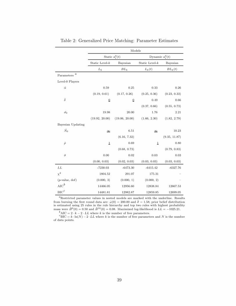
Table 2: Generalized Price Matching: Parameter Estimates

Models

Static a0i (t) Dynamic a0i (t)

Static Level-k Bayesian Static Level-k Bayesian

Lk BLk Lk(t) BLk(t)

Parametersa

Level-0 Players

α 0.59 0.25 0.33 0.26

(0.19, 0.61) (0.17, 0.26) (0.25, 0.36) (0.23, 0.33)

δ 0 0 0.49 0.66

(0.37, 0.66) (0.55, 0.73)

σ0 19.98 20.00 1.76 2.21

(19.92, 20.00) (19.06, 20.00) (1.66, 2.30) (1.82, 2.79)

Bayesian Updating

N0 ∞ 6.51 ∞ 10.23

(6.16, 7.32) (9.35, 11.87)

ρ 1 0.69 1 0.80

(0.68, 0.73) (0.79, 0.83)

σ 0.00 0.02 0.03 0.03

(0.00, 0.03) (0.02, 0.03) (0.03, 0.03) (0.03, 0.03)

LL -7230.03 -6473.30 -6415.42 -6327.76

χ2 1804.52 291.07 175.31 –

(p-value, dof) (0.000, 3) (0.000, 1) (0.000, 2) –

AICb

14466.05 12956.60 12838.84 12667.53

BICc

14481.81 12982.87 12859.85 12699.05

aRestricted parameter values in nested models are marked with the underline. Resultsfrom burning the first round data are: ω(0) = 200.00 and ˆσ = 1.58; prior belief distributionis estimated using 25 rules in the rule hierarchy and top two rules with highest probability

mass were B0(0) = 0.50 and B10(0) = 0.08. Maximized log-likelihood is LL = −1025.21.bAIC = 2 · k − 2 · LL where k is the number of free parameters.cBIC = k · ln(N)− 2 ·LL where k is the number of free parameters and N is the number

of data points.

39

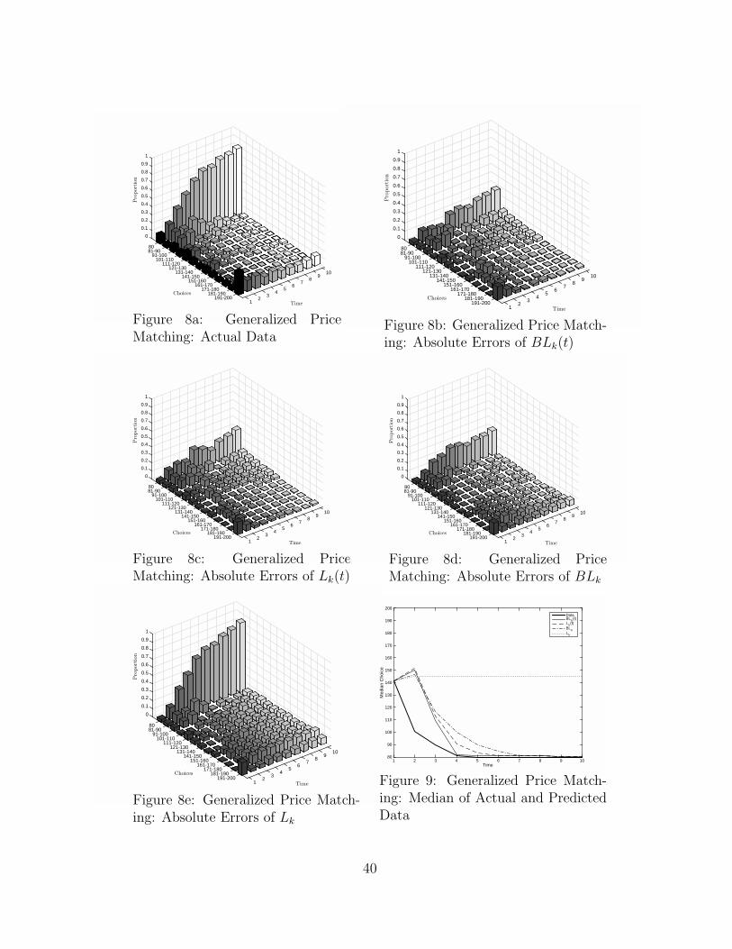
109

8 7

Time

6 5

4 3

2 1

191-200181-190

171-180161-170

151-160141-150

131-140

Choices

121-130111-120

101-11091-100

81-9080

1

0.9

0.8

0.7

0.6

0.5

0.4

0.3

0.2

0.1

0

Proportion

Figure 8a: Generalized PriceMatching: Actual Data

109

8 7

Time

6 5

4 3

2 1

191-200181-190

171-180161-170

151-160141-150

131-140

Choices

121-130111-120

101-11091-100

81-9080

1

0.9

0.8

0.7

0.6

0.5

0.4

0.3

0.2

0.1

0

Proportion

Figure 8b: Generalized Price Match-ing: Absolute Errors of BLk(t)

109

8 7

Time

6 5

4 3

2 1

191-200181-190

171-180161-170

151-160141-150

131-140

Choices

121-130111-120

101-11091-100

81-9080

1

0.9

0.8

0.7

0.6

0.5

0.4

0.3

0.2

0.1

0

Proportion

Figure 8c: Generalized PriceMatching: Absolute Errors of Lk(t)

109

8 7

Time

6 5

4 3

2 1

191-200181-190

171-180161-170

151-160141-150

131-140

Choices

121-130111-120

101-11091-100

81-9080

1

0.9

0.8

0.7

0.6

0.5

0.4

0.3

0.2

0.1

0

Proportion

Figure 8d: Generalized PriceMatching: Absolute Errors of BLk

109

8 7

Time

6 5

4 3

2 1

191-200181-190

171-180161-170

151-160141-150

131-140

Choices

121-130111-120

101-11091-100

81-9080

1

0.9

0.8

0.7

0.6

0.5

0.4

0.3

0.2

0.1

0

Proportion

Figure 8e: Generalized Price Match-ing: Absolute Errors of Lk

Time1 2 3 4 5 6 7 8 9 10

Med

ian

Cho

ice

80

90

100

110

120

130

140

150

160

170

180

190

200

DataBLk(t)Lk(t)BLkLk

Figure 9: Generalized Price Match-ing: Median of Actual and PredictedData

40

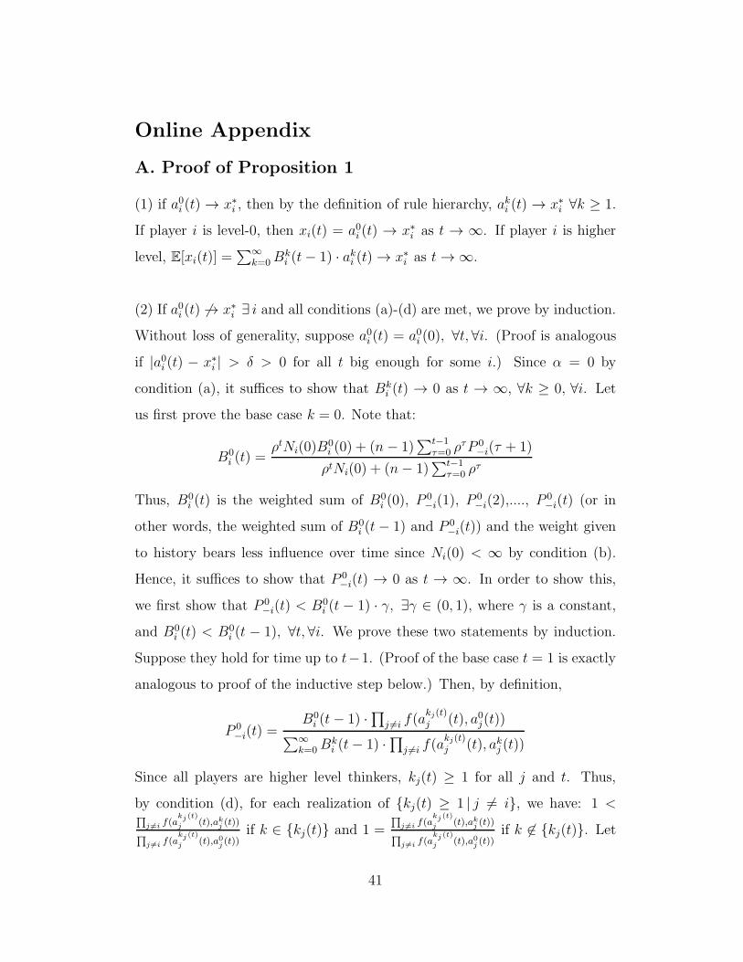
Online Appendix

A. Proof of Proposition 1

(1) if a0i (t) → x∗i , then by the definition of rule hierarchy, aki (t) → x∗

i ∀k ≥ 1.

If player i is level-0, then xi(t) = a0i (t) → x∗i as t → ∞. If player i is higher

level, E[xi(t)] =∑∞

k=0Bki (t− 1) · aki (t) → x∗

i as t → ∞.

(2) If a0i (t) 6→ x∗i ∃ i and all conditions (a)-(d) are met, we prove by induction.

Without loss of generality, suppose a0i (t) = a0i (0), ∀t, ∀i. (Proof is analogous

if |a0i (t) − x∗i | > δ > 0 for all t big enough for some i.) Since α = 0 by

condition (a), it suffices to show that Bki (t) → 0 as t → ∞, ∀k ≥ 0, ∀i. Let

us first prove the base case k = 0. Note that:

B0i (t) =

ρtNi(0)B0i (0) + (n− 1)

∑t−1τ=0 ρ

τP 0−i(τ + 1)

ρtNi(0) + (n− 1)∑t−1

τ=0 ρτ

Thus, B0i (t) is the weighted sum of B0

i (0), P0−i(1), P

0−i(2),...., P

0−i(t) (or in

other words, the weighted sum of B0i (t− 1) and P 0

−i(t)) and the weight given

to history bears less influence over time since Ni(0) < ∞ by condition (b).

Hence, it suffices to show that P 0−i(t) → 0 as t → ∞. In order to show this,

we first show that P 0−i(t) < B0

i (t − 1) · γ, ∃γ ∈ (0, 1), where γ is a constant,

and B0i (t) < B0

i (t − 1), ∀t, ∀i. We prove these two statements by induction.

Suppose they hold for time up to t−1. (Proof of the base case t = 1 is exactly

analogous to proof of the inductive step below.) Then, by definition,

P 0−i(t) =

B0i (t− 1) ·

∏

j 6=i f(akj(t)j (t), a0j(t))

∑∞k=0B

ki (t− 1) ·

∏

j 6=i f(akj(t)j (t), akj (t))

Since all players are higher level thinkers, kj(t) ≥ 1 for all j and t. Thus,

by condition (d), for each realization of {kj(t) ≥ 1 | j 6= i}, we have: 1 <∏

j 6=i f(akj (t)

j (t),akj (t))∏

j 6=i f(akj (t)

j (t),a0j (t))if k ∈ {kj(t)} and 1 =

∏

j 6=i f(akj (t)

j (t),akj (t))∏

j 6=i f(akj (t)

j (t),a0j (t))if k 6∈ {kj(t)}. Let

41

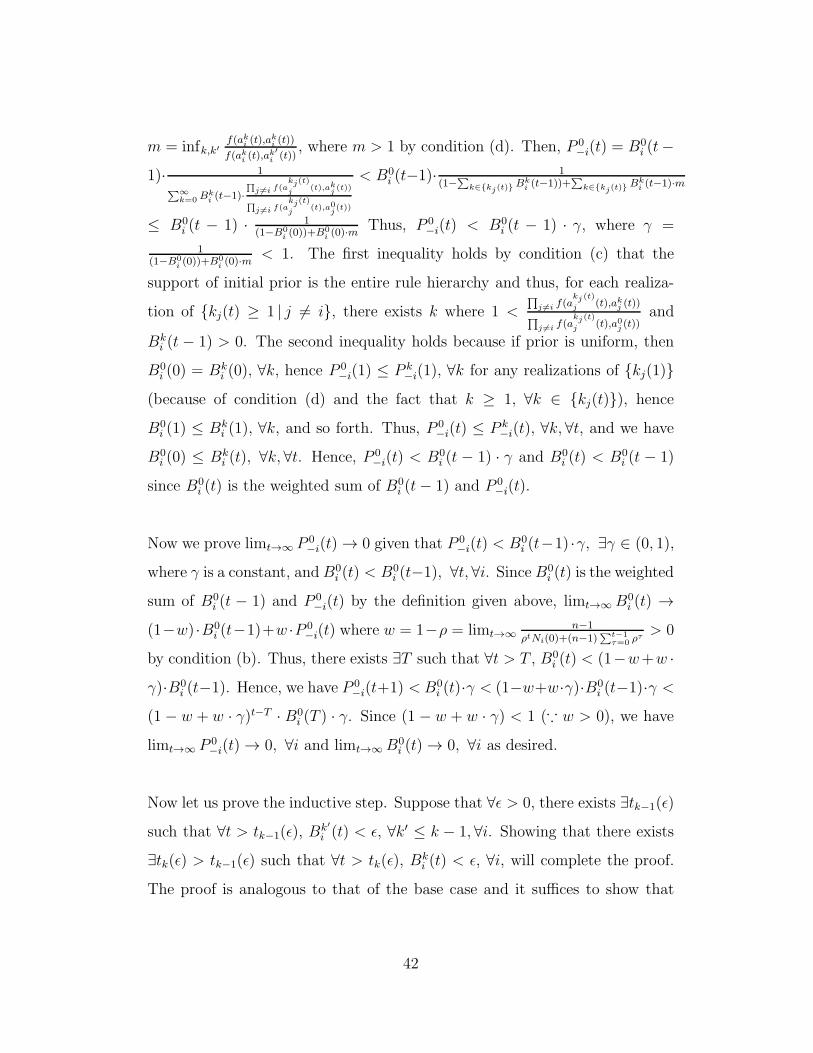
m = infk,k′f(aki (t),a

ki (t))

f(aki (t),ak′i (t))

, where m > 1 by condition (d). Then, P 0−i(t) = B0

i (t−

1)· 1

∑∞k=0 B

ki (t−1)·

∏j 6=i f(a

kj(t)

j(t),ak

j(t))

∏j 6=i f(a

kj(t)

j(t),a0

j(t))

< B0i (t−1)· 1

(1−∑

k∈{kj(t)}Bk

i (t−1))+∑

k∈{kj(t)}Bk

i (t−1)·m

≤ B0i (t − 1) · 1

(1−B0i (0))+B0

i (0)·mThus, P 0

−i(t) < B0i (t − 1) · γ, where γ =

1(1−B0

i (0))+B0i (0)·m

< 1. The first inequality holds by condition (c) that the

support of initial prior is the entire rule hierarchy and thus, for each realiza-

tion of {kj(t) ≥ 1 | j 6= i}, there exists k where 1 <∏

j 6=i f(akj (t)

j (t),akj (t))∏

j 6=i f(akj (t)

j(t),a0

j(t))

and

Bki (t − 1) > 0. The second inequality holds because if prior is uniform, then

B0i (0) = Bk

i (0), ∀k, hence P 0−i(1) ≤ P k

−i(1), ∀k for any realizations of {kj(1)}

(because of condition (d) and the fact that k ≥ 1, ∀k ∈ {kj(t)}), hence

B0i (1) ≤ Bk

i (1), ∀k, and so forth. Thus, P 0−i(t) ≤ P k

−i(t), ∀k, ∀t, and we have

B0i (0) ≤ Bk

i (t), ∀k, ∀t. Hence, P 0−i(t) < B0

i (t − 1) · γ and B0i (t) < B0

i (t − 1)

since B0i (t) is the weighted sum of B0

i (t− 1) and P 0−i(t).

Now we prove limt→∞ P 0−i(t) → 0 given that P 0

−i(t) < B0i (t−1) ·γ, ∃γ ∈ (0, 1),

where γ is a constant, andB0i (t) < B0

i (t−1), ∀t, ∀i. Since B0i (t) is the weighted

sum of B0i (t − 1) and P 0

−i(t) by the definition given above, limt→∞ B0i (t) →

(1−w) ·B0i (t−1)+w ·P 0

−i(t) where w = 1−ρ = limt→∞n−1

ρtNi(0)+(n−1)∑t−1

τ=0 ρτ> 0

by condition (b). Thus, there exists ∃T such that ∀t > T , B0i (t) < (1−w+w ·

γ)·B0i (t−1). Hence, we have P 0

−i(t+1) < B0i (t)·γ < (1−w+w·γ)·B0

i (t−1)·γ <

(1 − w + w · γ)t−T · B0i (T ) · γ. Since (1 − w + w · γ) < 1 (∵ w > 0), we have

limt→∞ P 0−i(t) → 0, ∀i and limt→∞B0

i (t) → 0, ∀i as desired.

Now let us prove the inductive step. Suppose that ∀ǫ > 0, there exists ∃tk−1(ǫ)

such that ∀t > tk−1(ǫ), Bk′

i (t) < ǫ, ∀k′ ≤ k − 1, ∀i. Showing that there exists

∃tk(ǫ) > tk−1(ǫ) such that ∀t > tk(ǫ), Bki (t) < ǫ, ∀i, will complete the proof.

The proof is analogous to that of the base case and it suffices to show that

42

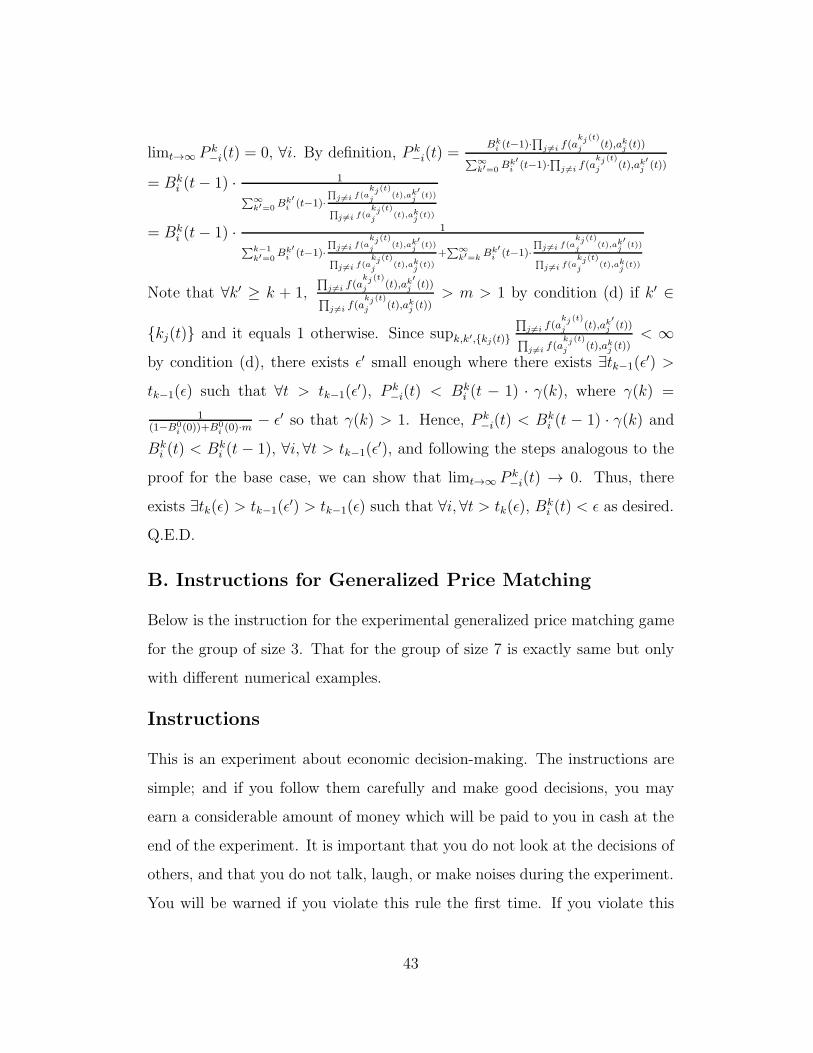
limt→∞ P k−i(t) = 0, ∀i. By definition, P k

−i(t) =Bk

i (t−1)·∏

j 6=i f(akj (t)

j (t),akj (t))∑∞

k′=0Bk′

i (t−1)·∏

j 6=i f(akj (t)

j (t),ak′

j (t))

= Bki (t− 1) · 1

∑∞k′=0

Bk′i (t−1)·

∏j 6=i f(a

kj(t)

j(t),ak

′j

(t))

∏j 6=i f(a

kj(t)

j(t),ak

j(t))

= Bki (t− 1) · 1

∑k−1k′=0

Bk′i (t−1)·

∏j 6=i f(a

kj(t)

j(t),ak

′j

(t))

∏j 6=i f(a

kj(t)

j(t),ak

j(t))

+∑∞

k′=kBk′

i (t−1)·

∏j 6=i f(a

kj(t)

j(t),ak

′j

(t))

∏j 6=i f(a

kj(t)

j(t),ak

j(t))

Note that ∀k′ ≥ k + 1,∏

j 6=i f(akj (t)

j (t),ak′

j (t))∏

j 6=i f(akj (t)

j (t),akj (t))> m > 1 by condition (d) if k′ ∈

{kj(t)} and it equals 1 otherwise. Since supk,k′,{kj(t)}

∏

j 6=i f(akj (t)

j (t),ak′

j (t))∏

j 6=i f(akj (t)

j (t),akj (t))< ∞

by condition (d), there exists ǫ′ small enough where there exists ∃tk−1(ǫ′) >

tk−1(ǫ) such that ∀t > tk−1(ǫ′), P k

−i(t) < Bki (t − 1) · γ(k), where γ(k) =

1(1−B0

i (0))+B0i (0)·m

− ǫ′ so that γ(k) > 1. Hence, P k−i(t) < Bk

i (t − 1) · γ(k) and

Bki (t) < Bk

i (t − 1), ∀i, ∀t > tk−1(ǫ′), and following the steps analogous to the

proof for the base case, we can show that limt→∞ P k−i(t) → 0. Thus, there

exists ∃tk(ǫ) > tk−1(ǫ′) > tk−1(ǫ) such that ∀i, ∀t > tk(ǫ), B

ki (t) < ǫ as desired.

Q.E.D.

B. Instructions for Generalized Price Matching

Below is the instruction for the experimental generalized price matching game

for the group of size 3. That for the group of size 7 is exactly same but only

with different numerical examples.

Instructions

This is an experiment about economic decision-making. The instructions are

simple; and if you follow them carefully and make good decisions, you may

earn a considerable amount of money which will be paid to you in cash at the

end of the experiment. It is important that you do not look at the decisions of

others, and that you do not talk, laugh, or make noises during the experiment.

You will be warned if you violate this rule the first time. If you violate this

43

rule twice, you will be asked to leave the room immediately and your cash

earnings will be $0.

The experiment consists of 10 decision rounds. In each decision round, you will

be randomly assigned into groups of 3 participants. That is, you are randomly

matched with other participants in each round, and your paired members may

be different round by round.

Experimental Procedure

In each decision round, all members in each group are asked to choose a num-

ber simultaneously between 80 and 200 (inclusive of 80 and 200, and up to

1 decimal point). Specifically, each member can choose any number among

80.0, 80.1, 80.2,., 199.8, 199.9, and 200.0. Note that each member must make

a choice without knowing what his or her paired members will choose. Once

all members in a group make their choices, the computer will determine each

members point earning based on everyones chosen number. Ones point earn-

ing is determined by ones chosen number and the minimum choice of ones

paired members excluding oneself. Details of how point earning is determined

will be given below. After each decision round, each participant will be told

(a) his/her choice in that round, (b) the minimum choice of his/her paired

members excluding him/herself in that round, and (c) his/her point earning

in that round. Again, every participant will undertake this task 10 times, and

will be randomly matched with other participants in each round.

Determination of Point Earnings

Your total point earning in each round is the sum of 2 components: baseline

earning and supplementary earning. Specifically, we have:

TOTAL POINT EARNING = BASELINE EARNING + SUPPLEMENTARY EARNING.

44

1. BASELINE EARNING: In each round, the baseline earning in a group is

given by the minimum of all members choices in that group. That is, we

will examine all choices in each group and use the minimum of the choices

in the group to determine its baseline earning. Note that all members

in a group receive the same baseline earning. Different groups, however,

may receive different baseline earnings depending on the choices of their

respective group members.

2. SUPPLEMENTARY EARNING: Depending on the relative magnitude be-

tween your own choice and the minimum of your paired members choices,

your supplementary earning can be either positive, negative, or zero. Each

case is described in full detail below.

(a) Positive Supplementary Earning: You will receive a positive supple-

mentary earning (on top of your baseline earning) if your own choice

is smaller than the minimum choice of your paired members excluding

yourself. This means that your choice is the only smallest number in

the group. That is, you have chosen the lowest number, while all your

paired members have chosen bigger numbers than you did. Since you

receive a positive supplementary earning, your total point earning will

be higher than your baseline earning as a consequence.

Precisely, your positive supplementary earning is 1.5 TIMES the dif-

ference between your choice and the minimum of your paired mem-

bers choices. However, there is a cap on the maximum supplementary

earning that you can earn. In this experiment, you can earn up to 15

supplementary points. Again, your total earning is the sum of your

baseline earning and supplementary earning.

(b) Negative Supplementary Earning: You will receive a negative supple-

45

mentary earning (i.e., a deduction from your baseline earning) if your

choice is higher than the minimum choice of your paired members ex-

cluding yourself. This means that someone else in your group has

chosen a smaller number than you did, and your choice is NOT the

lowest number (or the minimum). Since you receive a negative sup-

plementary earning, your total point earning will be lower than your

baseline earning as a consequence.

Precisely, the magnitude of your negative supplementary earning is 1.5

TIMES the difference between your choice and the minimum of your

paired members choices. However, there is a cap on the maximum

supplementary points that will be deducted from your baseline earning.

In this experiment, up to 15 supplementary points can be deducted

from your baseline earning. Again, your total earning is the sum of

your baseline earning and supplementary earning.

(c) No Supplementary Earning: You will receive no supplementary earning

if your choice is the smallest in your group, but there are also other

paired members who have chosen the same number as well. As a

consequence, your total point earning will simply be your baseline

earning.

46

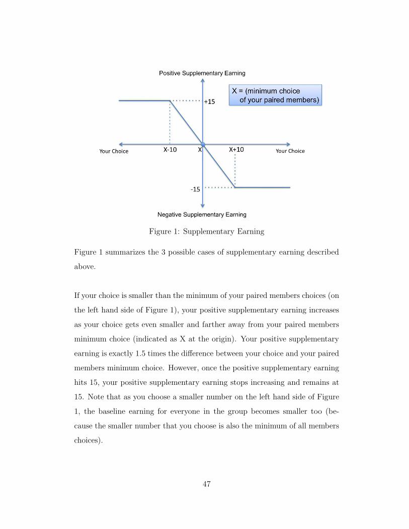
Figure 1: Supplementary Earning

Figure 1 summarizes the 3 possible cases of supplementary earning described

above.

If your choice is smaller than the minimum of your paired members choices (on

the left hand side of Figure 1), your positive supplementary earning increases

as your choice gets even smaller and farther away from your paired members

minimum choice (indicated as X at the origin). Your positive supplementary

earning is exactly 1.5 times the difference between your choice and your paired

members minimum choice. However, once the positive supplementary earning

hits 15, your positive supplementary earning stops increasing and remains at

15. Note that as you choose a smaller number on the left hand side of Figure

1, the baseline earning for everyone in the group becomes smaller too (be-

cause the smaller number that you choose is also the minimum of all members

choices).

47

If your choice is higher than the minimum of your paired members choices (on

the right hand side of Figure 1), you will receive a negative supplementary

earning. The magnitude of your negative supplementary earning increases

as your choice gets even higher and farther away from the minimum of your

paired members choices (indicated as X at the origin). The magnitude of your

negative supplementary earning is exactly 1.5 times the difference between

your choice and your paired members minimum choice. Likewise, once the

negative supplementary earning hits −15, it stops getting larger and remains

at −15. Note that as you choose a higher number on the right hand side of

Figure 1, the baseline earning for everyone in the group remains the same at

the minimum of your paired members choices (i.e., X) because X remains the

minimum of all members choices.

Finally, if your choice is the same as the minimum of your paired members

choices (when your choice is at the origin of Figure 1), your supplementary

earning is zero, and your total earning is simply the baseline earning.

Illustrative Examples

The numbers used in following examples are chosen purely for illustrative pur-

poses.

EXAMPLE 1: Assume your paired members chose 160.0 and 167.2, respec-

tively. Note that the minimum of your paired members choices is 160.0 (the

smaller of 160.0 and 167.2). We shall use Figure 2 below (which we created

by relabeling Figure 1) to determine your supplementary earning depending

on possible choices you can make. Note that the origin is now set to l60.

48

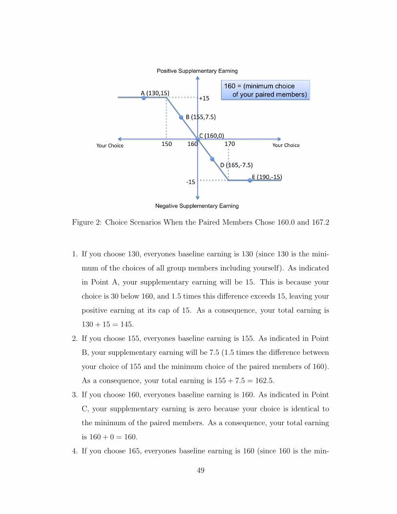
Figure 2: Choice Scenarios When the Paired Members Chose 160.0 and 167.2

1. If you choose 130, everyones baseline earning is 130 (since 130 is the mini-

mum of the choices of all group members including yourself). As indicated

in Point A, your supplementary earning will be 15. This is because your

choice is 30 below 160, and 1.5 times this difference exceeds 15, leaving your

positive earning at its cap of 15. As a consequence, your total earning is

130 + 15 = 145.

2. If you choose 155, everyones baseline earning is 155. As indicated in Point

B, your supplementary earning will be 7.5 (1.5 times the difference between

your choice of 155 and the minimum choice of the paired members of 160).

As a consequence, your total earning is 155 + 7.5 = 162.5.

3. If you choose 160, everyones baseline earning is 160. As indicated in Point

C, your supplementary earning is zero because your choice is identical to

the minimum of the paired members. As a consequence, your total earning

is 160 + 0 = 160.

4. If you choose 165, everyones baseline earning is 160 (since 160 is the min-

49

imum of choices of all group members including yourself). As indicated in

Point D, your supplementary earning will be −7.5. This is because your

choice is 5 above 160, and 1.5 times this difference is 7.5. As a consequence,

your total earning is 160− 7.5 = 152.5.

5. If you choose 190, everyones baseline earning is 160. As indicated in Point

E, your supplementary earning will be −15, because 1.5 times the difference

between your choice and the minimum of the paired members choices is 45

which exceeds 15. As a consequence, your total earning is 160− 15 = 145.

Table 1 summarizes the baseline, supplementary and total point earnings for

the 5 possible scenarios (when the paired members choose 160.0 and 167.2).

YourChoice

Point Indicatedin Figure 2

Your Paired Members’Minimum Choice

BaselineEarning

SupplementaryPoint Earning

Total PointEarning

130.0 A 160.0 130.0 +15.0 145.0

155.0 B 160.0 155.0 +7.5 162.5

160.0 C 160.0 160.0 0 160.0

165.0 D 160.0 160.0 -7.5 152.5

190.0 E 160.0 160.0 -15.0 145.0

Table 1: Summary of Earnings when the Paired Members Chose 160.0 and 167.2

EXAMPLE 2: Assume your paired members chose 120.0 and 147.8, respec-

tively. Note that the minimum of your paired members choices is 120.0 (the

smaller of 120.0 and 147.8). We shall use Figure 3 below (which we created

by relabeling Figure 1) to determine your supplementary earning depending

on possible choices you can make. Note that the origin is now set to l20.

50

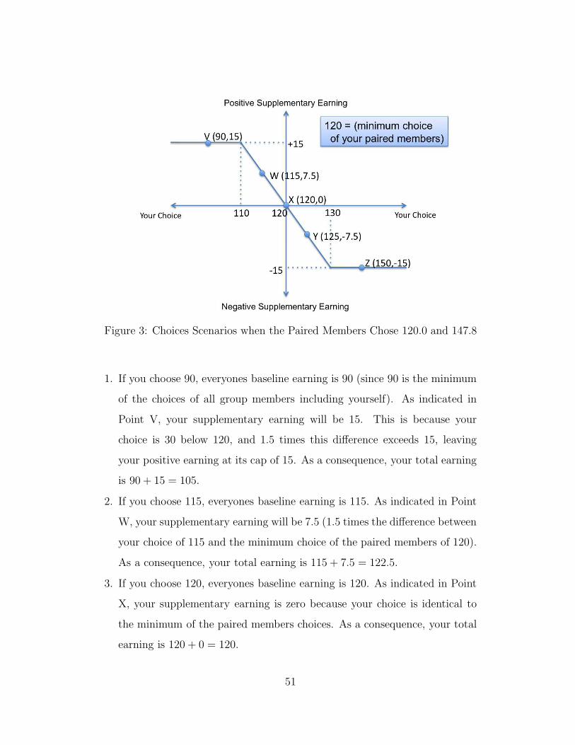
Figure 3: Choices Scenarios when the Paired Members Chose 120.0 and 147.8

1. If you choose 90, everyones baseline earning is 90 (since 90 is the minimum

of the choices of all group members including yourself). As indicated in

Point V, your supplementary earning will be 15. This is because your

choice is 30 below 120, and 1.5 times this difference exceeds 15, leaving

your positive earning at its cap of 15. As a consequence, your total earning

is 90 + 15 = 105.

2. If you choose 115, everyones baseline earning is 115. As indicated in Point

W, your supplementary earning will be 7.5 (1.5 times the difference between

your choice of 115 and the minimum choice of the paired members of 120).

As a consequence, your total earning is 115 + 7.5 = 122.5.

3. If you choose 120, everyones baseline earning is 120. As indicated in Point

X, your supplementary earning is zero because your choice is identical to

the minimum of the paired members choices. As a consequence, your total

earning is 120 + 0 = 120.

51

4. If you choose 125, everyones baseline earning is 120 (since 120 is the min-

imum of choices of all group members including yourself). As indicated in

Point Y, your supplementary earning will be −7.5. This is because your

choice is 5 above 120, and 1.5 times this difference is 7.5. As a consequence,

your total earning is 120− 7.5 = 112.5.

5. If you choose 150, everyones baseline earning is 120. As indicated in Point

Z, your supplementary earning will be −15 because 1.5 times the difference

between your choice and the minimum of the paired members choices is 45,

which exceeds 15. As a consequence, your total earning is 120− 15 = 105.

Table 2 summarizes the baseline, supplementary and total point earnings for

the 5 possible scenarios (when the paired members choose 120 and 147.8).

YourChoice

Point Indicatedin Figure 3

Your Paired Members’Minimum Choice

BaselineEarning

SupplementaryPoint Earning

Total PointEarning

90.0 V 120.0 90.0 +15.0 105.0

115.0 W 120.0 115.0 +7.5 122.5

120.0 X 120.0 120.0 0 120.0

125.0 Y 120.0 120.0 -7.5 112.5

150.0 Z 120.0 120.0 -15.0 105.0

Table 2: Summary of earnings when the paired members chose 120.0 and 147.8

Your Dollar Payoffs

At the end of the experiment, we will sum your point earning in each round

to obtain your total point earning over 10 rounds. We will then multiply your

total point earning by $0.01 to obtain your dollar earning. In addition, we will

add to this dollar earning $5 show-up fee to determine your final dollar earning.

The amount will be paid to you in cash before you leave the experiment today.

52