mathematics

Article

A Backward Technique for Demographic Noise inBiological Ordinary Differential Equation Models

Margherita Carletti 1,* and Malay Banerjee 2

1 Department DISPeA, University of Urbino Carlo Bo, 61029 Urbino (Pu), Italy2 Indian Institute of Technology Kanpur, Kanpur 208016, India; malayb@iitk.ac.in* Correspondence: margherita.carletti@uniurb.it

Received: 1 November 2019; Accepted: 4 December 2019; Published: 9 December 2019�����������������

Abstract: Physical systems described by deterministic differential equations represent idealizedsituations since they ignore stochastic effects. In the context of biomathematical modeling, wedistinguish between environmental or extrinsic noise and demographic or intrinsic noise, forwhich it is assumed that the variation over time is due to demographic variation of two or moreinteracting populations (birth, death, immigration, and emigration). The modeling and simulation ofdemographic noise as a stochastic process affecting units of populations involved in the model iswell known in the literature, resulting in discrete stochastic systems or, when the population sizes arelarge, in continuous stochastic ordinary differential equations and, if noise is ignored, in continuousordinary differential equation models. The inverse process, i.e., inferring the effects of demographicnoise on a natural system described by a set of ordinary differential equations, is still an issue to beaddressed. With this paper, we provide a technique to model and simulate demographic noise goingbackward from a deterministic continuous differential system to its underlying discrete stochasticprocess, based on the framework of chemical kinetics, since demographic noise is nothing but thebiological or ecological counterpart of intrinsic noise in genetic regulation. Our method can, thus, beapplied to ordinary differential systems describing any kind of phenomena when intrinsic noise is ofinterest.

Keywords: biomathematical modelling; demographic noise; chemical kinetics

1. Introduction

Physical systems are usually modeled by differential equations, either ordinary (ODEs) or delay(DDEs) or partial (PDEs). These models represent idealized situations, as they ignore stochastic effects.By incorporating random elements in a differential equation model, a system of stochastic differentialequations (SDEs), either stochastic ordinary (SODEs) or stochastic delay (SDDEs) or stochastic partialdifferential equations (SPDEs), respectively, arises. Stochastic models arise if we assume that a physicalsystem operates in a noisy environment or if we wish to study the noisy behavior in the systemsthemselves, for example the intrinsic variability of interaction between individuals of two or morecompeting species. In the first case, deterministic differential equation models are enhanced by theintroduction of some kind of noise processes modeling environmental fluctuations and lead to stochasticdifferential equation models. In the context of biomathematical modeling, we should distinguishbetween environmental or external noise and demographic or internal noise, for which it is assumedthat the variation over time is due to demographic variation of two or more interacting populations(birth, death, immigration, and emigration) and not due to environmental variation. The populationscould represent predator-prey interaction, competition, mutualism, or a single population dividedinto sub-populations of susceptible and infected individuals. On the other hand, external noise canarise from random fluctuations of one or more model parameters around some given mean value or

Mathematics 2019, 7, 1204; doi:10.3390/math7121204 www.mdpi.com/journal/mathematics

Mathematics 2019, 7, 1204 2 of 16

from stochastic fluctuations of the system around any of the equilibrium points, in which cases theresulting stochastic systems have multiplicative noise. Fluctuations in experimental data, instead, resultin additive noise stochastic systems.

An important point with stochastic models is also the understanding of the effects of randomnessas drivers for stability. The stability theory for stochastic (either ordinary, delay, or partial) differentialequations can be much richer than that for deterministic differential equations. The works by Mao [1–3]showed that environmental noise can have the effect of stabilization of an unstable system allowing tostate a number of theorems on stochastic asymptotic stability where the Lyapunov functions may not bepositive definite nor the generating operators of Lyapunov functions positive definite. The same authorshowed that another important feature of stochastic models in population dynamics is that environmentalnoise can suppress deterministic explosion.

Other than Biomathematics, randomness plays a crucial role when we try to model and simulateinteractions among molecular species in single cells in Computational Cell Biology. In order tounderstand the functioning of an organism, the network of interactions between genes, mRNAs,miRNAs, proteins and other molecules needs to be addressed. Genetic (Gene) Regulation, relyingon chemical kinetics theory, is the specific field that comes into play. In this case, cells are seen asbiochemical reactors in which low reactant numbers can lead to significant statistical fluctuationsin molecule numbers and reaction rates. These fluctuations are intrinsic: they are determinedby the reaction parameters and connectivity of the underlying biochemical networks. In fact, insingle cells, “molecular interactions produce stochastic fluctuations that may dominate cellulardynamics” [4]. Therefore, the modeling of molecular interactions in single cells requires the useof stochastic biochemical systems, which give a probabilistic description of cellular dynamics, andsuitable simulation methods must be used.

Moreover, dynamical features such as oscillations or bi-stability cannot be observed as the effectsof external (environmental) noise and the appropriate way to model them is to assume that intrinsicnoise is affecting the system. The discrete stochastic methods we use do not follow individual moleculesover time: they track only total molecular numbers. This leads to algorithms that describe the timeevolution of a discrete nonlinear Markov process [5,6]. Gillespie first conceived a rigorous mathematicalmodeling framework through the Stochastic Simulation Algorithm [7]. Unfortunately, the originalGillespie algorithm was computationally very intensive; thus, refinements of it were introduced bymany authors in order to reduce the computation time in simulations [8–12]. Gillespie [8] introducedthe τ-leap and midpoint τ-leap methods where the sampling of most likely reactions was taken froma Poisson distribution, Tian and Burrage [9] proposed the sampling from a Binomial distribution andCao et al. [10–12] introduced new strategies for the choice of the step size in τ-leap methods usingPoisson τ-leaping.

A definite acceleration of the simulation process, though, can only be done by turning to thecontinuous stochastic system obtained by considering the ∆t→ 0 limit of the discrete Markov process,leading to a system of stochastic ordinary differential equations (SODEs).

The modeling and simulation of demographic (intrinsic) noise in biological, ecological andbiochemical systems have been addressed by many authors, among whom are Smith and Trevino[13], who studied demographic stochasticity in bacteriophage parasitism of a host bacteria,Mandal et al. [14], who addressed the problem of demographic noise in phytoplankton allelopathy,and Carletti et al. [15], who constructed a stochastic model for the regulation of gene PTEN implied inmalignant brain tumours. All of these approaches have one feature in common, i.e., they start fromconsidering the phenomenon from its intrinsic discrete nature, then go onward to the continuousstochastic setting, and finally result in a deterministic ODEs system. What is still lacking in theliterature is an inverse method, i.e., a method to understand the impact of intrinsic noise when theonly known dynamics is given by an ordinary differential system. With this paper, we intend to fillthis gap by providing a technique that can reveal the effects of intrinsic/demographic noise startingfrom an ODEs model and going backwards to the discrete stochastic system. Our technique relies

Mathematics 2019, 7, 1204 3 of 16

on the stochastic modeling and simulation of Gene Regulatory Networks (GRNs) by considering theinvolved biological species as they were reactants of a chemically reacting system.

2. Materials and Methods

In order to elucidate the novel technique for finding the effects of intrinsic noise starting froman ordinary differential system, we consider a biological model for phage-bacteria interaction in anopen marine environment. The choice is due to the fact that all the analytical properties of the modelare well known from the paper by Beretta and Kuang [16] and that, when we address intrinsic noise inthe form of demographic noise, we are interested in stochasticity in birth and death rates, as well asproliferation and migration of biological or ecological populations.

Our technique is based on the theory developed in the field of chemical kinetics, according towhich an ODE model can be seen as the deterministic counterpart of the stochastic differential systemarising from the ∆t→ 0 limit of the discrete Markov process modeling the interaction between species,assuming them to be expressed by number of units instead of by concentration of populations. In ourframework, this theory can be seen as the “direct” method to approach demographic noise in naturalprocesses, assuming them to be inherently stochastic [5,17–19]. The method we introduce in thispaper, instead, is meant to give insights to demographic noise in an “inverse” or backward way, i.e.,assuming that only the deterministic behavior of the process is known and modeled by ordinarydifferential equations.

The outline of this article is the following:

• In Section 2.1 we provide a background to the modeling of gene regulation, pointing out the reasonwhy it is an intrinsically stochastic mechanism and describing the most common simulation techniques.

• In Section 2.2 we illustrate an example of modeling and simulation of a GRN in bacteriophage λ,based on the paper by Goutsias [20] and the simulation technique described in [17].

• In Section 2.3 we propose the novel technique through which we can study the effects of demographicnoise in the ODEs model by Beretta and Kuang [16], going backwards to the discrete stochasticprocess and the continuous stochastic system (characterised by SODEs) underlying the deterministicmodel.

2.1. Stochastic Modeling of Genetic Regulation

In molecular biology, the general transfers describe the normal flow of biological information: DNAcan be copied to DNA (DNA replication), DNA information can be copied into mRNA (messengerRNA), (transcription), and proteins can be synthesized using the information in mRNA as a template(translation).

A Genetic Regulatory Network is a collection of DNA segments in a cell that interact with eachother and with other substances in the cell, thereby governing the rates at which genes in the networkare transcribed into mRNA. Regulation of gene expression, or gene regulation, refers to the cellularcontrol of the amount and timing of changes to the appearance of the functional product of a gene.

The mechanisms that act on gene expression, i.e., the ability of a gene to produce a biologicallyactive protein, are based on biochemical processes that are inherently stochastic and are much morecomplex in eukaryotes than in prokaryotes. A major difference is that in eukaryotes there is the presenceof the nuclear membrane, which prevents the simultaneous transcription and translation that occursin prokaryotes [21]. Whereas, in prokaryotes, control of transcriptional initiation is the major pointof regulation, in eukaryotes the regulation of gene expression can be controlled from many differentpoints. In eukaryotes, transcriptional regulation tends to involve combinatorial interactions betweenseveral transcription factors. By “regulation” of transcription, we mean when transcription occurs andhow much RNA is created.

The simulation of a discrete chemical reacting system must be done through Stochastic SimulationAlgorithms (SSA), in which we assume low and integer molecular numbers. The first SSA is dueto Gillespie [7] and is a rigorous procedure for numerically simulating the evolution of a set of

Mathematics 2019, 7, 1204 4 of 16

chemical reactions in a (well-stirred) homogeneous chemical reacting system, by taking into accountthe randomness inherent in such a system. If S1, S2, . . . , SN represent N interacting molecular speciesthrough M reaction channels, then the evolution of such a system is characterized by a discretenonlinear Markov process in which a vector X(t) of dimension N, representing numbers (integervalues) of the N molecular species at time t, is evolved through time. The state vector X(t) is adiscrete jump Markov process, where the time evolution equation describing the probability that,given X(t0) = x0, then X(t) = x, i.e., P(x, t|x0, t0) is called the Chemical Master Equation (CME) andcan be written as

∂

∂tP(x, t|x0, t0) =

M

∑j=1

(aj(x− νj)P(x− νj, t|x0, t0)− aj(x)P(x, t|x0, t0)). (1)

This discrete parabolic partial differential equation is generally too difficult to solve (eitheranalytically or numerically) and different methods are needed to simulate its solution.

Any method to solve a system of chemical reactions is uniquely characterized by two sets ofquantities: the stoichiometric vectors ν1, . . . , νM which represent, in turn, the update of the numbersof molecules in the system if reactions R1, . . . , RM occur, respectively, and a set of M propensityfunctions a1(X(t)), . . . , aM(X(t), that describe the relative probabilities of reactions R1, . . . , RMoccurring, respectively.

The SSA is an essentially exact variable time step procedure, where “exact” means that it generatesthe same probability distribution as the CME. At each step, two random variables are sampled froma uniform density function U[0,1] in order to choose which reaction will occur and what length the timestep will have. The chemical species are then upgraded according to the corresponding stoichiometricvector, and the process is repeated until the simulation time range is covered. The crucial point withSSA is that the time step can become very small if the number of molecules of some reactant species islarge, and it is difficult to guarantee that the simulation proceeds one reaction at a time. SSA is, thus,a computationally demanding approach that avoids its applicability when (large) reaction networksare needed to model biologically realistic phenomena.

The point with it is the multiscale nature of the underlying problem. First, some reactions are muchfaster than others and rapidly reach a stable state. In the SSA, the dynamics of the system are driven bythe slow reactions. In a deterministic setting, this issue is called “stiffness”. Second, if some chemicalspecies are present in relatively small quantities, then modeling by a discrete stochastic process isappropriate, whereas, if other species appear in large quantities, then stochastic or deterministicdifferential equations are better tools to use. In the SSA, instead, all the species are considered asdiscrete stochastic processes [10].

Burrage et al. [18] addressed the issue of multiscale modeling by extending the approach ofHaseltine and Rawlings in [22] in classifying slow, intermediate and fast reactions to slow, intermediate,and fast regimes, resulting in a completely general, adaptive, and partitioning approach for thestochastic simulation of multiscaled systems involving chemical reactions.

Finally, the issue of non-homogeneity, typical of in vivo conditions, has been considered, amongothers, in the papers by Berry [23], Schnell and Turner [24], and Nicolau and Burrage [25]. All ofthese authors use Monte Carlo simulations on a two-dimensional lattice. In particular, Nicolau andBurrage [25] introduced the Anomalous Stochastic Simulation Algorithm (ASSA) that proved to bean effective and efficient algorithm to simulate the anomalous diffusion when the environment is notwell-mixed, due to the obstacles present within the cell, such as fixed proteins or cytoskelatal structures.

However, the SSA has been successfully applied to simulate, for example, the regulation oflambda phage [26], circadian rhythms [27,28], and many other kinds of GRNs.

When noise effects are still important but continuity arguments hold, by the application of theCentral Limit Theorem and by matching the first two moments of the CME, we can write an SODE

Mathematics 2019, 7, 1204 5 of 16

that describes the continuous time evolution of the Markov process X(t) involved in the SSA [29].This equation is sometimes called the Chemical Langevin Equation (CLE) and takes the form

dX(t) =M

∑j=1

νjaj(X(t))dt + B(X(t))dW(t), X(0) = X0, (2)

where W(t) = (W1(t), . . . , WN(t))′ is an N dimensional vector in which its individual elements areindependent Wiener processes and B(X(t)) is a N × N matrix satisfying

B2(X(t)) = C(X(t)) = νDiag(a1(X(t)), . . . , aM(X(t)))νT , (3)

where ν = [ν1, . . . , νM] is the N ×M stoichiometric matrix.Equation (2) is an Ito SODE representing the continuous stochastic evolution equation describing

intrinsic noise.Finally, when large numbers of molecules are taken into account so that we can talk about

concentrations, the deterministic continuous setting holds. This averaged behavior is described byan ODE of initial value type of the form

X′(t) =M

∑j=1

νjaj(X(t)), X(0) = X0. (4)

This is the standard regime of chemical kinetics where the Law of Mass Action applies.

2.2. An Example of Genetic Regulation in Bacteriophage λ

A known and simple model organism is that of bacteriophage λ, which is a virus that infects thebacterium E. coli and can take two forms: lysis or lysogen. In the lysogen state, the virus replicatespassively whenever E. coli replicates. Under appropriate conditions, a state change from lysogento lysis can be induced. Many mathematical models have been developed to describe the geneticregulatory behavior of λ. These include both deterministic [30] and stochastic [26,31] kinetics models.

Most of these models consider the behavior of the λ right operator control system and the actionof regulatory proteins, CI repressor and Cro. The right operator region OR consists of three bindingsites which are situated between the promoters PRM and PI for genes CI and Cro. The dimeric formsof repressor and Cro bind to these binding sites to regulate transcription [32]. The lysogenic state ismainly regulated by the PRM promoter and the CI gene, while lysis is mainly regulated by the PRpromoter of the Cro gene. Shea and Ackers [33] have given a detailed model based on 40 possibleconfigurations of OR.

We consider the model introduced by Goutsias [20], based on the simplified situation of onlytwo operating sites in OR. Goutsias views this as a restricted model of the transcription regulation ofthe repressor protein CI in which the operator site OR1 is absent. The model consists of ten reactionsand six unknowns: M (monomer protein), D (dimer transcription factor), RNA (mRNA produced bytranscription), DNA (free of dimers), DNA1 (bound by D at binding site OR1), and DNA2 (bound atsites OR1 and OR2 ).

Mathematics 2019, 7, 1204 6 of 16

The network can be described by the following reactions:

DNA1 → RNA + DNA1RNA → RNA + M

M → 0RNA → 0

M + M → DD → M + M

DNA + D → DNA1DNA1 → DNA + D

DNA1 + D → DNA2DNA2 → DNA1 + D,

(5)

where

• reaction 1 models transcription to mRNA occurring when D occupies OR1 ;• reactions 2, 3, 4 model mRNA translated into proteins and the decay of both;• reaction 5 models protein dimerizing to the transcription factor D;• reactions 6, 7, 8 model activation of transcription of M when D binds at OR1 ;• reactions 9 and 10 model prevention of the RNA polymerase from binding at the promoter region

and repression of transcription when D binds at OR2 .

The rate constant corresponding to reaction j is denoted by cj.According to the method used in [17] for modeling first order, second order, and homodimeric

reactions, we use variables Xi(t), i = 1, . . . , 6, to characterize the molecular state of the transcriptionalregulatory system at time t ≥ 0, where Xi(t) = (M, D, RNA, DNA, DNA1, DNA2). From the Goutsiasmodel (5), we obtain the following propensity functions aj(X)), j = 1, . . . , 10, and the stoichiometricvectors νj, j = 1, . . . , 10

a1(X) = c1X5

a2(X) = c2X3

a3(X) = c3X1

a4(X) = c4X3

a5(X) = c5X21

a6(X) = c6X2

a7(X) = c7X2X4

a8(X) = c8X5

a9(X) = c9X2X5

a10(X) = c10X6

ν1 = [0, 0, 1, 0, 0, 0]ν2 = [1, 0, 0, 0, 0, 0]ν3 = [−1, 0, 0, 0, 0, 0]ν4 = [0, 0, −1, 0, 0, 0]ν5 = [−2, 1, 0, 0, 0, 0]ν6 = [2, −1, 0, 0, 0, 0]ν7 = [0, −1, 0, −1, 1, 0]ν8 = [0, 1, 0, 1, −1, 0]ν9 = [0, −1, 0, 0, −1, 1]ν10 = [0, 1, 0, 0, 1, −1].

(6)

We initialize the system with m ≥ 1 monomers and d ≥ 1 dimers, and we assume g ≥ 1 DNAtemplates per cell. In this case, we have the initial state vector

X0 = (m, d, 0, g, 0, 0). (7)

Mathematics 2019, 7, 1204 7 of 16

The values of the specific probability rate constants cj in (6) are taken from relevant papers(see [20] and references therein) and are listed below:

c1 = 0.078c2 = 0.043c3 = 0.0007c4 = 0.0039c5 = 0.05 ∗ 109/AVc6 = 0.5c7 = 0.012 ∗ 109/AVc8 = 0.4791c9 = 0.00012 ∗ 109/AVc10 = 0.00021969,

(8)

where A = 6.0221415 ∗ 1023 mol−1 is the Avogadro number and V is the volume that, for simplicity,we assume constant and equal to 10−15. We set m = 2, d = 6, and assume that an average E. coli cell isinfected by about two λ chromosomes, i.e., g = 2.

For simulating the solution of the Goutsias discrete model (5), we used an enhancement of theGillespie SSA developed by the Kevin Burrage’s team in the years 2004–2006 (K.B, Tianhai Tian,Manuel Barrio, André Leier, Tatiana Marquez-Lago, and the first author of this paper) using a “sorting”algorithm, from now on addressed as the “sorting SSA”, that allows the speeding up of the performanceof the algorithm when choosing what reaction number should take place at every time step and usesa special time stepsize for monitoring and storing the updated concentrations of species [34].

We recall that, in a stochastic setting, we can provide either single simulations of just one strongsolution over a given path, or a number of independent simulations in order to collect informationabout mean behaviors. Since individual solutions are, however, representative of the dynamics of theprocesses being modeled, in Figure 1 that follow we will show single simulations of one strong solution.

Mathematics 2019, 7, 1204 8 of 16

0 100000

10

20

30

40

50

60

70

time

# m

ole

cu

les o

f M

(a)

0 100000

20

40

60

80

100

120

140

time

# m

ole

cu

les o

f D

(b)

0 100000

1

2

3

4

5

6

7

8

9

time

# m

ole

cu

les o

f R

NA

(c)

Figure 1. Numerical simulations of the first three components of solution state vector X(t) of theGoutsias model (5) via the sorting Stochastic Simulation Algorithm (SSA). (a) M(t), (b) D(t) and (c)RNA(t) (Time in minutes in the horizontal axis; number of molecules in the vertical axis).

2.3. Demographic Noise in Bacteriophage Infections: The Backward Gene Regulation Approach

Demographic noise in population dynamics and epidemic models has been studied by manyauthors with different approaches [5,14,35–38]. As already mentioned in the previous sections, in all ofthese approaches the starting system is discrete. Now, suppose we have an ODE model of differentkinds (biological, ecological, biochemical, etc.), and we wish to address the issue of how demographicnoise affects the underlying interacting species, in order to capture the intrinsic variability neglectedby the deterministic modeling. We consider the ODE model describing the dynamics of epidemicsinduced by bacteriophages in marine bacteria populations, introduced by Beretta and Kuang in [16].

Mathematics 2019, 7, 1204 9 of 16

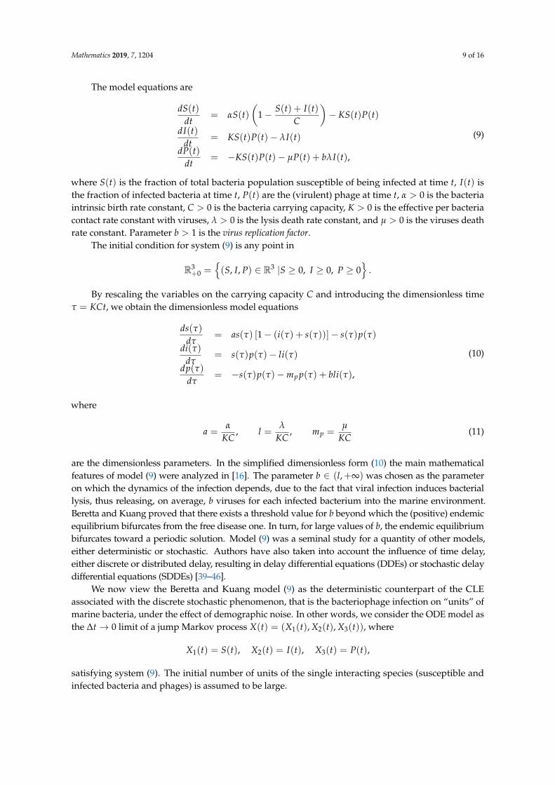
The model equations are

dS(t)dt

= αS(t)(

1− S(t) + I(t)C

)− KS(t)P(t)

dI(t)dt

= KS(t)P(t)− λI(t)dP(t)

dt= −KS(t)P(t)− µP(t) + bλI(t),

(9)

where S(t) is the fraction of total bacteria population susceptible of being infected at time t, I(t) isthe fraction of infected bacteria at time t, P(t) are the (virulent) phage at time t, α > 0 is the bacteriaintrinsic birth rate constant, C > 0 is the bacteria carrying capacity, K > 0 is the effective per bacteriacontact rate constant with viruses, λ > 0 is the lysis death rate constant, and µ > 0 is the viruses deathrate constant. Parameter b > 1 is the virus replication factor.

The initial condition for system (9) is any point in

R3+0 =

{(S, I, P) ∈ R3 |S ≥ 0, I ≥ 0, P ≥ 0

}.

By rescaling the variables on the carrying capacity C and introducing the dimensionless timeτ = KCt, we obtain the dimensionless model equations

ds(τ)dτ

= as(τ) [1− (i(τ) + s(τ))]− s(τ)p(τ)di(τ)

dτ= s(τ)p(τ)− li(τ)

dp(τ)dτ

= −s(τ)p(τ)−mp p(τ) + bli(τ),

(10)

where

a =α

KC, l =

λ

KC, mp =

µ

KC(11)

are the dimensionless parameters. In the simplified dimensionless form (10) the main mathematicalfeatures of model (9) were analyzed in [16]. The parameter b ∈ (l,+∞) was chosen as the parameteron which the dynamics of the infection depends, due to the fact that viral infection induces bacteriallysis, thus releasing, on average, b viruses for each infected bacterium into the marine environment.Beretta and Kuang proved that there exists a threshold value for b beyond which the (positive) endemicequilibrium bifurcates from the free disease one. In turn, for large values of b, the endemic equilibriumbifurcates toward a periodic solution. Model (9) was a seminal study for a quantity of other models,either deterministic or stochastic. Authors have also taken into account the influence of time delay,either discrete or distributed delay, resulting in delay differential equations (DDEs) or stochastic delaydifferential equations (SDDEs) [39–46].

We now view the Beretta and Kuang model (9) as the deterministic counterpart of the CLEassociated with the discrete stochastic phenomenon, that is the bacteriophage infection on “units” ofmarine bacteria, under the effect of demographic noise. In other words, we consider the ODE model asthe ∆t→ 0 limit of a jump Markov process X(t) = (X1(t), X2(t), X3(t)), where

X1(t) = S(t), X2(t) = I(t), X3(t) = P(t),

satisfying system (9). The initial number of units of the single interacting species (susceptible andinfected bacteria and phages) is assumed to be large.

Mathematics 2019, 7, 1204 10 of 16

By multiplying S(t) by the terms within parentheses in the first equation of model (9), we observethat seven reactions are taking place:

S → SS + S → 0S + I → IS + P → I

I → 0P → PI → P.

(12)

The associate propensity functions aj(X), the stoichiometric vectors νj, and reaction rates cj are

a1(X) = c1X1

a2(X) = c2X21

a3(X) = c3X1X2

a4(X) = c4X1X3

a5(X) = c5X2

a6(X) = c6X3

a7(X) = c7X2

ν1 = [1, 0, 0]ν2 = [−2, 0, 0]ν3 = [−1, 0, 0]ν4 = [−1, 1,−1]ν5 = [0,−1, 0]ν6 = [0, 0,−1]ν7 = [0, 0, 1]

c1 = α

c2 = α2C

c3 = αC

c4 = Kc5 = λ

c6 = µ

c7 = bλ.

(13)

Moreover, we know that the Chemical Langevin Equation associated to the discrete system (13)takes the form:

dX(t) =7

∑j=1

νjaj(X(t))dt + B(X(t))dW(t), X(0) = X0, (14)

where W(t) = (W1(t), . . . , WN(t))′ is a 3−dimensional vector whose individual elements areindependent Wiener processes and B(X(t)) is a 3× 3 matrix satisfying

B2(X(t)) = C(X(t)) = νDiag(a1(X(t)), . . . , a7(X(t)))νT , (15)

where ν = [ν1, . . . , ν7] is a 3× 7 stoichiometric matrix. We recall that Equation (14) is an Ito SODEand represents the continuous stochastic evolution equation modeling demographic (intrinsic) noisewithin system (12).

Using formulas (13), in Equation (14), matrix computations show that the 3× 7 stoichiometricmatrix C, satisfying B2(X(t)) = C(X(t)) = νDiag(a1(X(t)), . . . , a7(X(t)))νT and ν = [ν1, . . . , ν7]

(where B(X(t)) is a 3× 3 matrix), is

C =

a1 + 4a2 + a3 + a4 −a4 a4

−a4 a4 + a5 −a4

a4 −a4 a4 + a6 + a7

. (16)

All the numerical experiments presented in this paper were done on a last generation PC andcoded in MATLAB (R2019a) environment running under Windows 10.

3. Results

A thorough discussion of the analytical properties of the Beretta and Kuang ODEs model (9),including existence and uniqueness of the solution and the dependence of the dynamics of the modelon the phage replication number b, can be found in [16]. For our purposes, using a standard ODEsmethod for non-stiff differential equations, the simulations of the solution in continuous deterministicsetting result in Figure 2. Figure 2a shows that, if b is less than the critical value b∗ ≈ 16, only theboundary equilibrium E f = (C, 0, 0) exists. Susceptible bacteria reach their maximum value, whileinfected bacteria and phage vanish. Figure 2b,c show that for b∗ < b < bc, where a second critical value

Mathematics 2019, 7, 1204 11 of 16

bc ≈ 95, a globally stable positive equilibrium E+ = (S∗, I∗, P∗) exists, thus providing coexistence ofbacteria and phage. As a last case, Figure 2d shows that when b > bc, where bc is the bifurcation value,then a positive equilibrium exists but is unstable.

0 5 10 15 20 25 30 35 40 45 500

500

1000

1500

2000

2500

time

de

nsitie

s

Fast regime: ODEs

SIP

(a)

0 10 20 30 40 50 60 70 80 90 1000

500

1000

1500

2000

2500

3000

3500

time

de

nsitie

s

Fast regime: ODEs

SIP

(b)

0 1000 2000 3000 4000 5000 6000 7000 8000 9000 100000

0.5

1

1.5

2

2.5

3

3.5

4

4.5

5x 10

4

time

de

nsitie

s

Fast regime: ODEs

SIP

(c)

0 1000 2000 3000 4000 5000 6000 7000 8000 9000 100000

0.5

1

1.5

2

2.5

3

3.5

4

4.5

5x 10

4

time

de

nsitie

s

Fast regime: ODEs

SIP

(d)

Figure 2. Plots of the solution state vector (S(t), I(t), P(t)) (time in days in the horizontal axis; units ∗volume−1, volume in cm3, in the vertical axis) of the Beretta and Kuang ODEs model (9) for differentvalues of parameter b. (a) b = 15, (b) b = 20, (c) b = 94, and (d) b = 95.

If we apply the backward method described in Section 2.3 to the ODEs model (9), we obtain thediscrete stochastic system (12) and (13) modeling demographic noise in the phage-bacteria interactionand simulate the solutions via the sorting SSA. We expect that the more parameter b increases, themore the dynamics of the discrete system (12) and (13) is modified, accordingly to the continuous case.Figure 3 shows that the solutions fluctuate much more randomly with respect to the continuous model,particularly in the wide range of parameter b providing coexistence of the two species, i.e., b∗ < b < bc

(Figure 3b) and with respect to the phage population. Moreover, we note that the order of the solutions,

Mathematics 2019, 7, 1204 12 of 16

whatever b is, diminish by one when we turn from “concentrations” (continuous deterministic case) to“integer number of individuals” (discrete stochastic case).

0 10 20 30 40 50 600

200

400

600

800

1000

1200

time

nu

mb

er

SSA solver

S

I

P

(a)

0 10 20 30 40 50 600

200

400

600

800

1000

1200

time

nu

mb

er

SSA solver

S

I

P

(b)

0 2 4 6 8 10 12 14 160

1000

2000

3000

4000

5000

6000

time

nu

mb

er

SSA solver

S

I

P

(c)

Figure 3. Plots of the solution state vector (S(t), I(t), P(t)) (time in days in the horizontal axis; units ∗volume−1, volume in cm3, in the vertical axis) of the discrete phage-bacteria model in Equations (12)and (13), obtained by the sorting SSA for different values of parameter b. (a) b = 15, (b) b = 20, and (c)b = 95.

The simulations of system (12) and (13) with the SSA solver is, however, slow; thus, the integrationtime is much shorter than the integration time reached for the fast modeling regime via the ODEsystem (9). So, if we wish to know the long-time behavior of the stochastic biological system, wehave to consider the continuous stochastic regime represented by the Ito SODE (14). Using theEuler-Maruyama method for SODEs [41], we obtained Figure 4 confirming that even in the long-timebehavior parameter b is crucial: for low values of b, the solution still goes to the correspondingequilibrium state (Figure 4a), although more randomly than in the deterministic setting. For highervalues of b the effects of demographic noise, especially for the phage population, are much more

Mathematics 2019, 7, 1204 13 of 16

evident: the positive equilibrium E+ = (S∗, I∗, P∗) becomes unstable for values of parameter b muchsmaller than the deterministic bifurcation value bc = 94.451 (Figure 4b,c).

0 50 100 150 200 250 300 350 400 450 500

0

500

1000

1500

2000

2500

time

de

nsitie

s

Intermediate regime: SODEs

SIP

(a)

0 50 100 150 200 250 300 350 400 450 5000

500

1000

1500

2000

2500

3000

3500

4000

4500

5000

time

de

nsitie

s

Intermediate regime: SODEs

SIP

(b)

0 50 100 150 200 250 300 350 400 450 5000

0.5

1

1.5

2

2.5

3

3.5

4x 10

4

time

de

nsitie

s

Intermediate regime: SODEs

SIP

(c)

0 100 200 300 400 500 600 700 8000

1

2

3

4

5

6

7x 10

4

time

de

nsitie

s

Intermediate regime: SODEs

SIP

(d)

Figure 4. Plots of one path of the solution (S(t), I(t), P(t)) (time in days in the horizontal axis; units ∗volume−1, volume in cm3, in the vertical axis) of the SODEs model (14)–(16), obtained from the discretestochastic Goutsias model (5) when modeling demographic noise for different values of parameter b.(a) b = 15, (b) b = 20, (c) b = 60, and (d) b = 95. The Euler-Maruyama method is used.

We also note that the order of the solutions, for all values of parameter b, increases by one withrespect to the discrete stochastic case, thus regaining the same order of the original continuous, thoughdeterministic, setting.

4. Discussion

In this article, we provided a method to offer insights into deterministic differential modelswhen intrinsic noise is of interest. If the ordinary differential system is of biological or ecologicalnature, intrinsic noise is the so-called demographic noise. Our framework is that of chemical kinetics

Mathematics 2019, 7, 1204 14 of 16

used to model intrinsic noise involved in molecular biology, in particular, in genetic regulation usingSSAs. We first gave an example of application of the direct method for modeling demographicnoise to a gene regulation network in bacteriophage λ, using a particular type of SSA developed byBurrage et al. in [17,34,47]. Next, we inferred the effects of demographic noise on an ODEs modelof phage-bacteria interaction [16] going backward from the deterministic differential system to itsdiscrete stochastic counterpart, thus giving insights to the effects of randomly fluctuating birth anddeath rates, immigration and/or emigration of the involved molecular species. We observe that ourmethod is quite general and can be applied to ODE models of different nature, not only in life sciences.Unfortunately, at the moment its applicability is limited to ODEs where the underlying chemicalreaction channels are either first order, heterodimeric (second and higher order), homodimeric, andHill-type reactions for which a mathematical formulation can be provided, according to [17,19].

We are not able to compare our results with other authors’ results since, to our knowledge,no equivalent methods starting from the deterministic setting can be found in the literature.Nevertheless, it would be interesting to compare the outcomes of our backward method with thoseobtained by applying the direct method to the same biological process in such a way to evaluate therobustness of the backward technique. We expect that the two approaches (direct and inverse) lead tovery similar outcomes. Finally, a higher level of biological realism could be reached if, jointly withdemographic noise, we consider time delay, for example, for modeling incubation time or latencyperiod. In such a case, for the direct method, the Delay Stochastic Simulation Algorithm (DSSA)and the Delay Chemical Master Equation [15,34,48] would be the appropriate simulation tools to use.As with the backward (delay) method, there are good models to start with, for example, the Berettaand Kuang or the Beretta et al. [39,49] phage infection models with delay. All of these issues are beingaddressed in a new research article in preparation.

Author Contributions: software, M.C.; supervision, M.B.; Writing—original draft, M.C.

Funding: This research received no external funding.

Acknowledgments: Margherita Carletti is grateful to Kevin Burrage, QUT, Brisbane (Australia) for giving her theopportunity to take her PhD under his supervision and to Gaetano Zanghirati, University of Ferrara (Italy), forhis critical comments on the MATLAB codes used to perform the numerical experiments presented in this paper.Moreover, the authors wish to thank the reviewers for their precious help in improving the submitted paper.

Conflicts of Interest: The authors declare no conflict of interest.

References

1. Mao, X. Stochastic stabilization and destabilization. Syst. Control Lett. 1994, 23, 279–290. [CrossRef]2. Mao, X. Stochastic self-stabilization. Stoch. Stoch. Rep. 1996, 57, 57–70. [CrossRef]3. Mao, X. Some contributions to stochastic asymptotic stability and boundedness via multiple Lyapunov

functions. J. Math. Anal. Appl. 2001, 153, 325–340. [CrossRef]4. Elowitz, M.B.; Levine, A.J.; Siggia, E.D.; Swain, P.S. Stochastic gene expression in a single cell. Science 2002,

297, 1183–1186. [CrossRef] [PubMed]5. Allen, L.J.S. An Introduction to Stochastic Processes with Applications to Biology, 2nd ed.; Chapman Hall/CRC Press:

Boca Raton, FL, USA, 2003.6. Allen, L.J.S. Stochastic Population and Epidemic Models. Persistence and Extinction; Mathematical Biosciences

Lecture Series, Stochastics in Biological Systems; Springer: New York, NY, USA, 2015; Volume 1.3.7. Gillespie, D.T. A general method for numerically simulating the stochastic time evolution of coupled

chemical reactions. J. Comput. Phys. 1976, 22, 403–434. [CrossRef]8. Gillespie, D.T. Approximate accelerated stochastic simulation of chemically reacting systems. J. Chem. Phys.

2001, 115, 1716. [CrossRef]9. Tian, T.; Burrage, K. Binomial leap methods for simulating stochastic chemical kinetics. J. Chem. Phys. 2004,

121, 10356–10364. [CrossRef]10. Cao, Y.; Li, H.; Petzold, L. Efficient formulation of the stochastic simulation algorithm for chemically reacting

systems. J. Chem. Phys. 2004, 121, 4059–4067. [CrossRef]

Mathematics 2019, 7, 1204 15 of 16

11. Cao, Y.; Gillespie, D.T.; Petzold, L.R. Avoiding negative populations in explicit Poisson tau-leaping.J. Chem. Phys. 2005, 123, 054104. [CrossRef]

12. Cao, Y.; Gillespie, D.T.; Petzold, L.R. Efficient step size selection for the tau-leaping simulation method.J. Chem. Phys. 2006, 124, 044109. [CrossRef]

13. Smith, H.L.; Trevino, R.T. Bacteriophage Infection Dynamics: Multiple Host Binding Sites. Math. Model. Nat.Phenom. 2009, 4, 109–134. [CrossRef]

14. Mandal, P.S.; Allen, L.J.S.; Banerjee, M. Stochastic modeling of phytoplankton allelopathy. Appl. Math. Model.2014, 38, 1583–1596. [CrossRef]

15. Carletti, M.; Montani, M.; Meschini, V.; Radici, L.; Bianchi, M. Stochastic modeling of PTEN regulation inbrain tumors. A model for glioblastoma multiforme. Math. Biosci. Eng. 2015, 12, 965–981. [PubMed]

16. Beretta, E.; Kuang, Y. Modeling and analysis of a marine bacteriophage infection. Math. Biosci. 1998, 149,57–76. [CrossRef]

17. Burrage, K.; Tian, T. Effective simulation techniques for biological systems, in fluctuations and noise inbiological, biophysical, and biomedical systems II. In Proceedings of the SPIE—The International Society forOptical Engineering: Fluctuations and Noise in Biological, Biophysical, and Biomedical Systems II, Maspalomas, Spain,26–28 May 2004; SPIE: Bellingham, WA, USA, 2004; Volume 5467, pp. 311–325.

18. Burrage, K.; Tian, T.; Burrage, P.M. A multi-scaled approach for simulating chemical reaction systems.Prog. Biophys. Mol. Biol. 2004, 85, 217–234. [CrossRef]

19. Burrage, K.; Burrage, P.; Leier, A.; Marquez-Lago, T. A review of stochastic and delay simulation approachesin both time and space in computational cell biology. In Stochastic Processes, Multiscale Modeling, and NumericalMethods for Computational Cellular Biology; Holcman, D., Ed.; Springer: New York, NY, USA, 2017.

20. Goutsias, J. Quasiequilibrium approximation of fast reaction kinetics in stochastic biochemical sysmtems.J. Chem. Phys. 2005, 122, 184102. [CrossRef]

21. Choudhuri, S. Gene Regulation and Molecular Toxicology. Toxicol. Mech. Methods 2004, 15, 1–23. [CrossRef]22. Haseltine, E.L.; Rawlings, J.B. Approximate simulation of coupled fast and slow reactions for stochastic

chemical kinetics. J. Chem. Phys. 2002, 117, 6959–6969. [CrossRef]23. Berry, H. Monte-Carlo simulations of enzyme reactions in two dimensions: Fractal kinetics and spatial

segregation. Biophys. J. 2002, 83, 1891–1901. [CrossRef]24. Schnell, S.; Turner, T.E. Reaction kinetics in Intracellular environments with macromolecular crowding:

Simulations and rate laws. Prog. Biophysica Mol. Biol. 2004, 85, 235–260. [CrossRef]25. Nicolau, D.V., Jr.; Burrage, K. Stochastic simulation of chemical reactions in spatially complex media.

Comput. Math. Appl. 2008, 55, 1007–1018. [CrossRef]26. Arkin, A.; Ross, J.; McAdams, H.H. Stochastic kinetic analysis of developmental pathway bifurcation in

phage lambda-infected Escherichia coli cells. Genetics 1998, 149, 1633–1648. [PubMed]27. Elowitz, M.B.; Leibler, S. A synthetic oscillatory network of transcriptional regulators. Nature 2000, 403,

335–338. [CrossRef] [PubMed]28. Gonze, D.; Halloy, J.; Goldbeter, A. Robustness of circadian rythms with respect to molecular noise. Proc.

Natl. Acad. Sci. USA 2002, 99, 673–678. [CrossRef]29. Gillespie, D.T. A rigorous derivation of the chemical master equation. Physica A 1992, 188, 404–425. [CrossRef]30. Ackers, G.K.; Johnson, A.D.; Shea, M.A. Quantitative model for gene regulation by λ phage repressor. Proc.

Natl. Acad. Sci. USA 1982, 79, 1129–1133. [CrossRef]31. Hasty, J.; Pradines, J.; Dolnik, M.; Collins, J.J. Noise-based switches and amplifiers for gene expression. Proc.

Natl. Acad. Sci. USA 2000, 97, 2075–2080. [CrossRef]32. Ptashne, M. A Genetic Switch: Phage λ Revisited, 3rd ed.; Cold Spring Harbor Laboratory Press: Cold Spring

Harbor, NY, USA, 2004.33. Shea, M.A.; Ackers, G.K. The OR control system of bacteriophage Lambda: A physical-chemical model for

gene regulation. J. Mol. Biol. 1985, 181, 211–230. [CrossRef]34. Barrio, M.; Burrage, K.; Leier, A.; Tian, T. Oscillatory Regulation of Hes1: Discrete stochastic delay modeling

and simulation. PLoS Comput Biol. 2006, 2, e117. [CrossRef]35. Braumann, C.A. Environmental versus demographic stochasticity in population growth. In Workshop on

Branching Processes and Their Applications; González, M.V., Puerto, I.M., Martínez, R., Molina, M., Mota, M.,Ramos, A., Eds.; 37 Lecture Notes in Statistics—Proceedings; Springer: Berlin/Heidelberg, Germany, 2010;Volume 197.

Mathematics 2019, 7, 1204 16 of 16

36. Vieira dos Santos, R. Discreteness inducing coexistence. Physica A 2013, 392, 5888–5897. [CrossRef]37. Constable, G.W.A.; Rogers, T.; McKane, A.J.; Tarnita, C.E. Demographic noise can reverse the direction of

deterministic selection. Proc. Natl. Acad. Sci. USA 2016, 113, E4745–E4754. [CrossRef] [PubMed]38. Weissmann, H.; Shnerb, N.M.; Kessler, D.A. Simulation of spatial systems with demographic noise.

Phys. Rev. E 2018, 98, 022131. [CrossRef] [PubMed]39. Beretta, E.; Kuang, Y. Modeling and analysis of a marine bacteriophage infection with latency period.

Nonlin. Anal. RWA 2001, 2, 35–74. [CrossRef]40. Rabinovitch, A.; Aviramb, I.; Zaritsky, A. Bacterial debris—An ecological mechanism for coexistence of

bacteria and their viruses. J. Theor. Biol. 2003, 224, 377–383. [CrossRef]41. Buckwar, E. The Θ-Maruyama scheme for stochastic functional differential equations with distributed

memory term. Monte Carlo Methods Appl. 2004, 10, 235–244. [CrossRef]42. Gourley, S.A.; Kuang, Y. A stage structured predator-prey model and its dependence on maturation delay

and death rate. J. Math. Biol. 2004, 49, 188–200. [CrossRef]43. Gourley, S.A.; Kuang, Y. A delay reaction-diffusion model of the spread of bacteriophage infection.

SIAM J. Appl. Math. 2005, 65, 550–566. [CrossRef]44. Liu, S.; Liu, Z.; Tang, J. A delayed marine bacteriophage infection model. Appl. Math. Lett. 2007, 20, 702–706.

[CrossRef]45. Carletti, M. On the stability properties of a stochastic model for phage–bacteria interaction in open marine

environment. Math. Biosci. 2002, 175, 117–131. [CrossRef]46. Carletti, M. Mean-square stability of a stochastic model for bacteriophage infection with time delays.

Math. Biosci. 2007, 210, 395–414. [CrossRef]47. Leier, A.; Marquez-Lago, T.T.; Burrage, K. Generalized binomial Tau-leap method for biochemical kinetics

incorporating both delay and intrinsic noise. J. Chem. Phys. 2008, 128, 205107. [CrossRef] [PubMed]48. Tian, T.; Burrage, K.; Burrage, P.M.; Carletti, M. Stochastic delay differential equations for genetic regulatory

networks. J. Comp. Appl. Math. 2007, 205, 696–707. [CrossRef]49. Beretta, E.; Carletti, M.; Solimano, F. On the effects of environmental fluctuations in a simple model of

bacteria-bacteriophage interaction. Canad. Appl. Math. Quart. 2000, 8, 321–366.

c© 2019 by the authors. Licensee MDPI, Basel, Switzerland. This article is an open accessarticle distributed under the terms and conditions of the Creative Commons Attribution(CC BY) license (http://creativecommons.org/licenses/by/4.0/).