Morphological Grayscale Reconstruction in Image Analysis:

Applications and E�cient Algorithms

Luc Vincent

Abstract

Morphological reconstruction is part of a set of image operators often referred to as geodesic.In the binary case, reconstruction simply extracts the connected components of a binary imageI (the mask) which are \marked" by a (binary) image J contained in I. This transformationcan be extended to the grayscale case, where it turns out to be extremely useful for severalimage analysis tasks. This paper �rst provides two di�erent formal de�nitions of grayscalereconstruction. It then illustrates the use of grayscale reconstruction in various image processingapplications and aims at demonstrating the usefulness of this transformation for image �lteringand segmentation tasks. Lastly, the paper focuses on implementation issues: the standardparallel and sequential approaches to reconstruction are brie y recalled; their commondrawbackis their ine�ciency on conventional computers. To improve this situation, a new algorithmis introduced, which is based on the notion of regional maxima and makes use of breadth-�rst image scannings implemented via a queue of pixels. Its combination with the sequentialtechnique results in a hybrid grayscale reconstruction algorithm which is an order of magnitudefaster than any previously known algorithm.

Published in the IEEE Transactions on Image Processing, Vol. 2, No. 2, pp. 176{201,April 1993.

1

1 Introduction

Reconstruction is a very useful operator provided by mathematical morphology [18, 19]. Althoughit can easily be de�ned in itself, it is often presented as part as a set of operators known as geodesicones [7]. The reconstruction transformation is relatively well-known in the binary case, where itsimply extracts the connected components of an image which are \marked" by another image (seex 2). However, reconstruction can be de�ned for grayscale images as well. In this framework, itturns out to be particularly interesting for several �ltering, segmentation and feature extractiontasks. Surprisingly, it has attracted little attention in the image analysis community.

The present paper has three major goals: the �rst one is to provide a formal de�nition ofgrayscale reconstruction in the discrete case. In fact, we propose below two equivalent de�nitions:the �rst one is based on the threshold superposition principle and the second one relies on grayscalegeodesic dilations. The second part of the paper illustrates the use of binary and especially grayscalereconstruction in image analysis applications: examples proving the interest of grayscale reconstruc-tion for such tasks as image �ltering, extrema, domes and basins extraction in grayscale images,\top-hat" by reconstruction, binary and grayscale segmentation, etc., are discussed. Lastly, in x 4,we introduce e�cient algorithms for computing reconstruction in grayscale images. Up to now, theexecution times required by the known grayscale reconstruction algorithms make their practical userather cumbersome on conventional computers. Two algorithms are introduced to bridge this gap.The �rst one is based on the notion of regional maxima and uses breadth-�rst image scanningsenabled by a queue of pixels [25]. The second one is a combination of this scanning technique withthe classical sequential one [14], and it turns out to be the fastest algorithm in almost all practicalcases.

We shall exclusively be concerned here with the discrete case. The algorithms are describedin 2D, but their extension to images of arbitrary dimensions is straightforward. In order to be asprecise as possible, Vincent90:Thesis algorithm descriptions are done in a pseudo-langage whichbares similarities to C and Pascal.

2 De�nitions

2.1 Notations used throughout the paper

In the following, an image I is a mapping from a �nite rectangular subset DI of the discrete planeZZ

2 into a discrete set f0; 1; : : : N � 1g of gray-levels. A binary image I can only take values 0 or 1and is often regarded as the set of its pixels with value 1. In this paper, we often present notionsfor discrete sets of ZZ2 instead of explicitely referring to binary images. Similary, gray-level imagesare often regarded as functions or mappings.

The discrete grid G � ZZ2 � ZZ

2 provides the neighborhood relationships between pixels: pis a neighbor of q if and only if (p; q) 2 G. Here, we shall use square grids, either in 4- or in8-connectivity (see Fig. 1), or the hexagonal grid (see Fig. 2). Note however that the algorithmsdescribed below work for any grid, in any dimension. The distance induced by G on ZZ2 is denoteddG: dG(p; q) is the minimal number of edges of the grid to cross to go from pixel p to pixel q. In4-connectivity, this distance is often called city-block distance whereas in 8-connectivity, it is thechessboard distance [2]. The elementary ball in distance dG is denoted BG, or simply B. We denoteby NG(p) the set of the neighbors of pixel p for grid G. In the following, we often consider twodisjoined subsets of NG(p), denoted N

+G (p) and N

�G (p). N

+G (p) is the set of the neigbors of p which

are reached before p during a raster scanning of the image (left to right and top to bottom) andN�G (p) consists of the neighbors of p which are reached after p. These notions are recalled on Fig. 3.

2

(a) (b)

Figure 1: Portion of square grid in 4- (a) and 8-connectivity (b).

Figure 2: Portion of hexagonal grid.

(a)

(b)p

p

Figure 3: (a) The elementary ball B in 4-, 6- and 8-connectivity; (b) N+G (p) and

N�G (p) in 8-connectivity.

3

2.2 Reconstruction for binary images

2.2.1 De�nition in terms of connected components

Let I and J be two binary images de�ned on the same discrete domain D and such that J � I .In terms of mappings, this means that: 8p 2 D; J(p) = 1 =) I(p) = 1. J is called the markerimage and I is the mask. Let I1, I2, : : : , In be the connected components of I .

De�nition 2.1 The reconstruction �I(J) of mask I from marker J is the union of the connectedcomponents of I which contain at least a pixel of J:

�I(J) =[

J\Ik 6=;

Ik:

This de�nition is illustrated by Fig. 4. It is extremely simple, but gives rise to several interestingapplications and extensions, as we shall see in the following sections.

⇒

Figure 4: Binary reconstruction from markers.

2.2.2 De�nition in terms of geodesic distance

Reconstruction is most of the time presented using the notion of geodesic distance. Given a set X(the mask), the geodesic distance betweeen two pixels p and q is the length of the shortest pathsjoining p and q which are included in X . Note that the geodesic distance between two pixels withina mask is highly dependent on the type of connecticity which is used. This notion is illustrated byFig. 5. Geodesic distance was introduced in the framework of image analysis in 1981 by Lantu�ejouland Beucher [6] and is at the basis of several morphological operators [7]. In particular, one cande�ne geodesic dilations (and similarly erosions) as follows:

De�nition 2.2 Let X � ZZ2 be a discrete set of ZZ2 and Y � X. The geodesic dilation of size

n � 0 of Y within X is the set of the pixels of X whose geodesic distance to Y is smaller or equalto n:

�(n)X (Y ) = fp 2 X j dX(p; Y ) � ng:

From this de�nition, it is obvious that geodesic dilations are extensive transformations, i.e.

Y � �(n)X (Y ). In addition, geodesic dilation of a given size n can be obtained by iterating n

elementary geodesic dilations:

�(n)X (Y ) = �

(1)X � �

(1)X � : : : � �

(1)X| {z }

n times

(Y ): (1)

4

A

y

x

P

Figure 5: Geodesic distance dG(x; y) within a set A.

Fig. 6 illustrates successive geodesic dilations of a marker inside a mask, using 4- and 8-connectivity.The elementary geodesic dilation can itself be obtained via a standard dilation of size one followedby an intersection:

�(1)X (Y ) = (Y �B) \X: (2)

This last statement is absolutely wrong when non-elementary geodesic dilations are considered. Inthis latter case, one merely gets the conditional dilation of set Y , de�ned as the intersection of Xand the standard dilation of Y . Note that some authors use a di�erent terminology and utilize theword \conditional" for what this paper calls \geodesic" [5].

(a) 4-connectivity (b) 8-connectivity

Figure 6: Boundaries of the successive geodesic dilations of a set (in black) withina mask.

When performing successive elementary geodesic dilations of a set Y inside a mask X , theconnected components of X whose intersection with Y is non empty are progressively ooded. The

5

following proposition can thus be stated:

Proposition 2.3 The reconstruction of X from Y � X is obtained by iterating elementary geodesicdilations of Y inside X until stability. In other words:

�X(Y ) =[n�1

�(n)X (Y ):

This proposition is at the basis of one of the simplest algorithms for computing geodesic recon-structions in both the binary and the grayscale cases (see x 4.1).

2.3 Grayscale reconstruction

2.3.1 De�nition using threshold superposition

It has been known for several years that|at least in the discrete case|any increasing transforma-tion de�ned for binary images can be extended to grayscale images [18, 19, 31, 20]. By increasing,we mean a transformation such that

8X; Y � ZZ2; Y � X =) (Y ) � (X): (3)

In order to extend such a transformation to grayscale images I taking their values in f0; 1; : : : ; N�1g, it su�ces to consider the successive thresholds Tk(I) of I , for k = 0 to N � 1:

Tk(I) = fp 2 DI j I(p) � kg: (4)

They are said to constitute the threshold decomposition of I [10, 11]. As illustrated by Fig. 7, thesesets obviously satisfy the following inclusion relationship:

8k 2 [1; N � 1]; Tk(I) � Tk�1(I):

When applying the increasing operation to each of these sets, their inclusion relationships arepreserved. Thus, we can now extend to grayscale images as follows:

8p 2 DI ; (I)(p) = maxfk 2 [0; N � 1] j p 2 (Tk(I))g: (5)

In the present case, binary geodesic reconstruction is an increasing transformation in that itsatis�es:

Y1 � Y2; X1 � X2; Y1 � X1; Y2 � X2 =) �X1(Y1) � �X2

(Y2): (6)

Therefore, following the threshold superposition principle of equation (5), we de�ne grayscale re-construction as follows [27]:

De�nition 2.4 (grayscale reconstruction, �rst de�nition) Let J and I be two grayscale im-ages de�ned on the same domain, taking their values in the discrete set f0; 1; : : : ; N � 1g and suchthat J � I (i.e., for each pixel p 2 DI ; J(p) � I(p)). The grayscale reconstruction �I(J) of I fromJ is given by:

8p 2 DI ; �I(J)(p) = maxfk 2 [0; N � 1] j p 2 �Tk(I)(Tk(J))g:

Fig. 8 illustrates this transformation. Just like binary reconstruction extracts those connectedcomponents of the mask which are marked, grayscale reconstruction extracts the peaks of the maskwhich are marked by the marker-image. This characteristics is taken into account in the examplesof application presented in x 3.

6

Function "Pile" of sets

⇔

Figure 7: Threshold decomposition of a graylevel image.

f

g

⇒

Figure 8: Grayscale reconstruction of mask f from marker g.

7

2.3.2 Alternative de�nition of grayscale reconstruction

The former de�nition does not provide any interesting computational method to determine grayscalereconstruction in digital images. Indeed, even if a fully optimized binary reconstruction algorithmis used, one has to apply it 256 times to determine grayscale reconstruction for images on 8 bits!Therefore, it is most useful to introduce this transformation using the geodesic dilations presentedin section 2.2.2.

Following the threshold decomposition principle, one can easily de�ne the elementary geodesic

dilation �(1)I (J) of grayscale image J � I \under" I :

�(1)I (J) = (J �B) ^ I; (7)

In this equation, ^ stands for the pointwise minimum and J � B is the dilation of J by atstructuring element B [18, 19]. These two notions are the direct extension to the grayscale case ofrespectively intersection and binary dilation by B. The grayscale geodesic dilation of size n � 0 isthen given by:

�(n)I (J) = �

(1)I � �

(1)I � : : : � �

(1)I| {z }

n times

(J): (8)

This leads to a second de�nition of grayscale reconstruction:

De�nition 2.5 (grayscale reconstruction, second de�nition) The grayscale reconstruction�I(J) of I from J is obtained by iterating grayscale geodesic dilations of J \under" I until sta-bility is reached, i.e.:

�I(J) =_n�1

�(n)I (J):

It is straightforward to verify that both this de�nition and de�nition 2.4 correspond to the sametransformation.

Similarly, the elementary geodesic erosion "(1)I (J) of grayscale image J � I \above" I is given

by

"(1)I (J) = (J B) _ I; (9)

where _ stands for the pointwise maximum and JB is the erosion of J by at structuring elementB [18, 19]. The grayscale geodesic erosion of size n � 0 is then given by:

"(n)I (J) = "

(1)I � "

(1)I � : : : � "

(1)I| {z }

n times

(J): (10)

We are now able to de�ne the dual grayscale reconstruction in terms of geodesic erosions:

De�nition 2.6 (dual reconstruction) Let I and J be two grayscale images de�ned on the samedomain DI and such that I � J. The dual grayscale reconstruction ��I(J) of mask I from markerJ is obtained by iterating grayscale geodesic erosions of J \above" I until stability is reached:

��I(J) =^n�1

"(n)I (J):

3 Applications

In this section, we underscore the tremendous interest of binary and grayscale reconstruction inimage analysis. Surprisingly enough, reconstruction is not a very well-known transformation, par-ticularly in the grayscale case. The examples presented below provide a non-exhaustive catalog ofapplications of reconstruction in image analysis.

8

3.1 Filtering by opening-reconstruction

In the binary case, the opening by a disc (or other types of structuring elements) is commonly usedto �lter out the image parts which cannot hold the disc. Recall that the opening of a binary imageI by a disc is the union of all the possible positions of the disc when it is totally included in theimage I [18, 28].

In some cases, one wishes to �lter out all the connected components which cannot contain thedisc while preserving the others entirely. The way to do so is to reconstruct the original image I fromits opening by the disc. The resulting transformation is often called opening by reconstruction andbelongs to the category of the algebraic openings [20]. An example is shown on Fig. 9: after openingby a disc of radius 2, several connected components of the original image have been removed, butthe shape of some of the remaining ones has been dramatically modi�ed. After reconstruction, theoriginal shape of the not totally removed particles is restaured. Opening by reconstruction extendsto the grayscale case in a straightforward manner. It turns out to be a particularly interestingoperation, especially when large structuring elements are used in the opening step.

(a) original image (b) opening by a disc of radius 2 (c) reconstructed image

Figure 9: Use of opening by reconstruction for �ltering.

3.2 Use of top-hat by reconstruction for segmentation

Let us now illustrate on an example one of the possible uses of grayscale reconstruction for picturesegmentation: Fig. 10.a represents an angiography of eye blood vessels in which microaneurismshave to be detected. They are small compact light spots which are disconnected from the networkof the (light) blood vessels and mainly located in the dark central area of the image. Obviously,it is impossible to detect these micro-aneurisms via simple thresholdings. Similarly, a top-hattransformation [12] consisting in subtracting from the original image its morphological openingwith respect to a small disc would extract all the \white" features, i.e. aneurisms and bloodvessels, which is not desirable.

To correctly segment these micro-aneurisms, one has to account for the fact that they are com-pact whereas the blood vessels are elongated. A series of morphological openings of Fig. 10.a withrespect to segments of di�erent orientations is thus performed. These segments are chosen to belonger than any possible aneurism, so that all the aneurisms are removed by any such opening. Onthe other hand, there will be at least one orientation for which the vessels are not completely re-moved by opening. After taking the supremum of these di�erent openings, one gets Fig. 10.b, whichis still an algebraic opening of Fig. 10.a [19]. It is used as marker to reconstruct the blood vessels

9

entirely. Fig. 10.c is the result of the grayscale reconstruction of Fig. 10.a from Fig. 10.b. Sincethe aneurisms are disconnected from the blood vessels, they have not been reconstructed! Thus, byalgebraic di�erence between Fig. 10.a and Fig. 10.c, followed by a relatively simple thresholding, themicroaneurisms shown in Fig. 10.d are extracted. The succession of operations used for the presentsegmentation task is an extension of the family of the top-hat transformations, often referred to astop-hat by reconstruction.

3.3 Regional maxima and dome extraction

Reconstruction turns out to provide a very e�cient method to extract regional maxima and minimafrom grayscale images. Furthermore, the technique extends to the determination of \maximalstructures", which we call h-domes and h-basins. Let us �rst brie y review the notion of regionalmaximum:

De�nition 3.1 (regional maximum) A regional maximum M of a grayscale image I is a con-nected components of pixels with a given value h (plateau at altitude h), such that every pixel inthe neighborhood of M has a strictly lower value.

Regional maxima should not be mistaken with local maxima. Recall that a pixel p of I is a localmaximum for grid G if and only if its value I(p) is greater or equal to that of any of its neighbors.All the pixels belonging to a regional maximum are local maxima, but the converse is not true: forexample, a pixel p belonging to the inside of a plateau is a local maximum, but the plateau mayhave neighboring pixels of higher altitude and thus not be a regional maximum.

An alternative de�nition can also be proposed for the notion of regional maximum [23]:

De�nition 3.2 A regional maximum at altitude h of grayscale image I is a connected componentC of Th(I) such that C \ Th+1(I) = ;.

(Recall from eq. (4) that Th(I) is threshold of I at level h.)Determining the regional maxima of a grayscale image is relatively easy and several algorithms

have been proposed in literature, some of which are reviewed in [23]. One of the most e�cientmethods makes use of grayscale reconstruction and is based on the following proposition:

Proposition 3.3 The (binary) image M(I) of the regional maxima of I is given by:

M(I) = I � �I(I � 1):

proof : According to de�nition 3.2, a connected component C of Th(I) is a maximum at level hif and only if C \ Th+1(I) = C \ Th(I � 1) = ;. In other words, the set Mh of the pixelsbelonging to a maximum of I at altitude h is given by:

Mh = Th(I) n �Th(I)(Th(I � 1)): (11)

Now, for any h, h0, h 6= h0, Mh\Mh0 = ;. This means that by replacing the set di�erence (n)by an algebraic di�erence and using the threshold superposition principle, formula (11) canbe extended to the grayscale case. 2

This proposition is illustrated by Fig. 11.Now, instead of subtracting value 1 in prop. 3.3, an arbitrary gray-level constant h can be

subtracted from I . This provides a useful technique for extracting \domes" of a given height, thatwe call h-domes. The following de�nition can be proposed:

10

Microaneurisms

(a) (b)

(c) (d)

Figure 10: Use of grayscale reconstruction for image segmentation: (a) original im-age of blood vessels, (b) supremum of openings by segments, (c) recon-structed image, (d) microaneurisms obtained after substraction of (c)from (a) and thresholding step.

11

I

I-1grayscale

reconstruction⇒

Regional maxima

Figure 11: Extracting the regional maxima of I by reconstruction of I from I � 1.

De�nition 3.4 The h-dome image Dh(I) of the h-domes of a grayscale image I is given by:

Dh(I) = I � �I(I � h):

Geometrically speaking, an h-dome can be interpreted the same way maxima are: an h-dome D ofimage I is a connected component of pixels such that:� every pixel p neighbor of D satis�es: I(p) < minfI(q) j q 2 Dg,

� maxfI(q) j q 2 Dg �minfI(q) j q 2 Dg < h.In addition, the value of pixel p of h-dome D in image Dh(I) is equal to I(p)-minfI(q) j q 2 Dg.

The h-dome transformation is illustrated on Fig. 12. Unlike classical top-hats, the h-dometransformation extracts light structures without involving any size or shape criterion. The onlyparameter (h) is related to the height of these structures. This characteristic is of interest forcomplex segmentation problems.

I

I-h

Grayscale reconstruction

Subtraction

h

Figure 12: Determination of the h-domes of grayscale image I.

As an example, let us consider Fig. 13.a, which is an image of the corneal endothelial tissueof the eye, obtained using a wide-�eld specular microscope. The analysis of images of this kindis detailed in [29]. The �rst step of their segmentation consists in extracting a marker for each

12

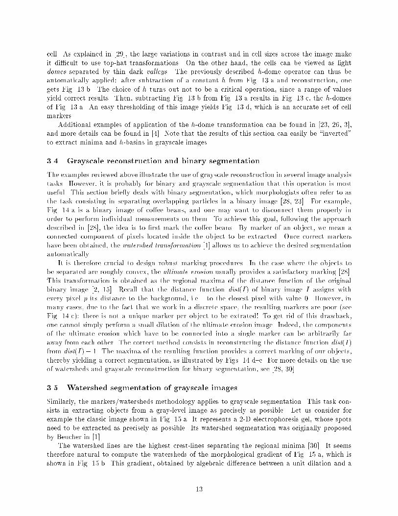
cell. As explained in [29], the large variations in contrast and in cell sizes across the image makeit di�cult to use top-hat transformations. On the other hand, the cells can be viewed as lightdomes separated by thin dark valleys. The previously described h-dome operator can thus beautomatically applied: after subtraction of a constant h from Fig. 13.a and reconstruction, onegets Fig. 13.b. The choice of h turns out not to be a critical operation, since a range of valuesyield correct results. Then, subtracting Fig. 13.b from Fig. 13.a results in Fig. 13.c, the h-domesof Fig. 13.a. An easy thresholding of this image yields Fig. 13.d, which is an accurate set of cellmarkers.

Additional examples of application of the h-dome transformation can be found in [23, 26, 3],and more details can be found in [4]. Note that the results of this section can easily be \inverted"to extract minima and h-basins in grayscale images.

3.4 Grayscale reconstruction and binary segmentation

The examples reviewed above illustrate the use of grayscale reconstruction in several image analysistasks. However, it is probably for binary and grayscale segmentation that this operation is mostuseful. This section brie y deals with binary segmentation, which morphologists often refer to asthe task consisting in separating overlapping particles in a binary image [28, 23]. For example,Fig. 14.a is a binary image of co�ee beans, and one may want to disconnect them properly inorder to perform individual measurements on them. To achieve this goal, following the approachdescribed in [28], the idea is to �rst mark the co�ee beans. By marker of an object, we mean aconnected component of pixels located inside the object to be extracted. Once correct markershave been obtained, the watershed transformation [1] allows us to achieve the desired segmentationautomatically.

It is therefore crucial to design robust marking procedures. In the case where the objects tobe separated are roughly convex, the ultimate erosion usually provides a satisfactory marking [28].This transformation is obtained as the regional maxima of the distance function of the originalbinary image [2, 15]|Recall that the distance function dist(I) of binary image I assigns withevery pixel p its distance to the background, i.e.. to the closest pixel with value 0. However, inmany cases, due to the fact that we work in a discrete space, the resulting markers are poor (seeFig. 14.c): there is not a unique marker per object to be extrated! To get rid of this drawback,one cannot simply perform a small dilation of the ultimate erosion image. Indeed, the componentsof the ultimate erosion which have to be connected into a single marker can be arbitrarily faraway from each other. The correct method consists in reconstructing the distance function dist(I)from dist(I)� 1. The maxima of the resulting function provides a correct marking of our objects,thereby yielding a correct segmentation, as illustrated by Figs. 14.d{e. For more details on the useof watersheds and grayscale reconstruction for binary segmentation, see [28, 30].

3.5 Watershed segmentation of grayscale images

Similarly, the markers/watersheds methodology applies to grayscale segmentation. This task con-sists in extracting objects from a gray-level image as precisely as possible. Let us consider forexample the classic image shown in Fig. 15.a. It represents a 2-D electrophoresis gel, whose spotsneed to be extracted as precisely as possible. Its watershed segmentation was originally proposedby Beucher in [1].

The watershed lines are the highest crest-lines separating the regional minima [30]. It seemstherefore natural to compute the watersheds of the morphological gradient of Fig. 15.a, which isshown in Fig. 15.b. This gradient, obtained by algebraic di�erence between a unit dilation and a

13

(a) original image (b) after grayscale reconstruction

(c) h-domes (d) cell markers

Figure 13: Extraction of cell markers in images of corneal endothelial tissue.

14

(a) original binary image I (co�ee beans) (b) level lines of distance function dist(I)

(c) ultimate erosion: poor markers (d) correct markers

(e) segmented image

Figure 14: Use of grayscale reconstruction in binary segmentation. The correctmarkers are obtained as the regional maxima of the reconstruction ofthe distance function dist(I) from dist(I)� 1.

15

unit erosion of Fig. 15.a, is shown in Fig. 15.b. The spot contours are located on crest-lines of thisgradient, but far too many of these crest lines are due to noise in the original data. Therefore, thewatersheds of Fig. 15.b yield the over-segmented result of Fig. 15.c.

As explained in numerous recent publications [28, 20, 30, 13], the correct way to use watershedsfor grayscale image segmentation consists in �rst detecting markers of the objects to be extracted.The design of robust marker detection techniques involves the use of knowledge speci�c to the seriesof images under study. Not only object markers, but also background markers need to be extracted.In the present case, describing the marking technique used for Fig. 15.a would go beyond the scopeof this paper. The extracted marker image is shown in Fig. 15.d.

After marker extraction, the rest of the segmentation can proceed automatically as follows:grayscale reconstruction is used to modify the gradient image G into an image G0 such that:� its only minima are located on the extracted markers,

� its highest crest-lines separating markers are preserved.More speci�cally, denote by G the gradient image and by M the binary marker image. Let mbe the maximal value of the pixels of G. The image G0 is de�ned as the dual reconstruction ofmin(G+ 1; (m+ 1)M) from (m+ 1)M (see de�nition. 2.6):

G0 = ��min(G+1;(m+1)M)((m+ 1)M): (12)

In this process, pixels located on markers are given value 0 in G0 and non-marked catchment basinsget �lled up. More details on this process are given in [28, 23, 20]. The resulting modi�ed gradient isshown in Fig. 15.e. Its watersheds now provide the desired segmentation, as illustrated by Fig. 15.f.This segmentation methodology is commonly used in morphology and has been successfully appliedto various types of images: NMR images [23], digital elevation models [21], corneal endothelialimages [29], succession of images used for motion estimation [3], and many others.

4 Computing reconstruction in digital images

In this section, we are concerned with both the binary and the grayscale case, but the emphasis is puton grayscale reconstruction. Indeed, in the binary case, a straightforward e�cient implementationof morphological reconstruction can be proposed as follows:

1. Label the connected components of the mask image, i.e., each of these components is assigneda unique number. Note that this step can itself be implemented very e�ciently by usingalgorithms based on chain and loops [16] or queues of pixels [23, 26].

2. Determine the labels of the connected components which contain at least a pixel of the markerimage

3. Remove all the connected components whose label is not one of the previous ones.

As mentioned earlier, such an algorithm could be extended to the grayscale case by working on thedi�erent thresholds of the images. However, it would be extremely ine�cient, making grayscalereconstruction a too cumbersome transformation to be used in practice. This is the reason whywe are now interested in implementing this transformation as e�ciently as possible. Note howeverthat the algorithms described below also work in the binary case if one considers binary imagesas grayscale images taking only values 0 and 1. In the algorithm descriptions of this section, ' 'refers to the assignment symbol.

16

(a) original image (b) morphological gradient

(c) watersheds of gradient (d) markers of spots and background

(e) modi�ed gradient (f) �nal segmentation

Figure 15: Watershed segmentation of 2-D electrophoresis gels.

17

4.1 Standard technique

Proposition 2.3 and de�nition 2.5 directly yield a computational technique for determining grayscalereconstruction in digital images. The corresponding algorithm is part of a set of classical methodsreferred to as parallel ones [23, 25, 26]. It basically works by iterating elementary dilation followedby pointwise minimum until stability as follows:

Algorithm: parallel reconstruction

� I: mask image (binary or grayscale)

� J: marker image, defined on domain DI, J � I.Reconstruction is determined directly in J

� Allocate work image K defined on DI

� Repeat until stability (i.e. no more pixel value modifications):

� Dilation step: for every pixel p 2 DI

� K(p) maxfJ(q); q 2 NG(p)[ fpgg

� Pointwise minimum: For every pixel p 2 DI

� J(p) min(K(p); I(p))

In each of the above steps, the image pixels can be scanned in an arbitrary order, so that theimplementation of this algorithm on a parallel machine is extremely easy and e�cient. However,it requires the iteration of numerous complete image scannings, sometimes several hundreds! It istherefore not suited to conventional computers, where its execution time is often of several minutes.

4.2 Sequential reconstruction algorithm

In an attempt to reduce the number of scannings required for the computation of an image trans-form, sequential or recursive algorithms have been proposed [14]. They rely on the following twoprinciples:

� the image pixels are scanned in a prede�ned order, generally raster or anti-raster,

� the new value of the current pixel, determined from the values of the pixels in itsneighborhood, is written directly in the same image, so that it is taken into accountwhen determining the new values of the as yet unconsidered pixels.

Here, unlike for parallel algorithms, the scanning order is essential! This type of algorithm was�rst introduced for the computation of distance functions [15] and then extended to a numberof morphological transformations [8, 23]. Among others, binary and grayscale reconstruction canbe obtained sequentially by using the following algorithm, where information is �rst propagateddownwards in a raster scanning and then upwards in an anti-raster scanning.

Algorithm: sequential reconstruction

� I: mask image (binary or grayscale)

� J: marker image, defined on domain DI, J � I.Reconstruction is determined directly in J

18

� Repeat until stability:

� Scan DI in raster order:

� Let p be the current pixel;

� J(p) �maxfJ(q); q 2 N+

G (p) [ fpgg�^ I(p)

� Scan DI in anti-raster order:

� Let p be the current pixel;

� J(p) �maxfJ(q); q 2 N�

G (p) [ fpgg�^ I(p)

This algorithms usually only requires a few image scannings (a dozen typically) until stability isreached, and is therefore much more e�cient than the parallel algorithm presented in the previoussection. However, like several other sequential algorithms [26], it does not deal well with \rolled-upstructures" (connected components in the binary case and crest-lines in the grayscale case): asillustrated by Fig. 16 in the binary case, the sequential reconstruction of a rolled-up componentmay require several complete image scannings in which the value of only very few pixels is actuallymodi�ed.

X

Y

1. 2. 3.

4. 5. 6.

Figure 16: The sequential computation of a binary reconstruction in a rolled up maskmay involve several complete image scannings: here, the hatched zonesrepresent the pixels which have been modi�ed after each step.

4.3 Regional maxima and reconstruction

As detailed in [25, 26], a further step in the design of e�cient morphological processing consistsin trying to consider only the pixels whose value may be modi�ed. A �rst scanning is used todetect the pixels which are the process initiators and are typically located on the boundaries of theobjects or regions of interest. Then, starting from these pixels, information is propagated only inthe relevant image parts. Two categories of algorithms relying on this principle have been proposedin literature: the �rst ones are based on the encoding of the objects boundaries as loops and thepropagation of these structures in the image or in some given mask [16], whereas the algorithms of

19

the second category regard the images under study as graphs and realize breadth-�rst scannings ofthese graphs starting from strategically located pixels [23, 26, 22]. These two class of methods canbe used to e�ciently implement such complex morphological operations as propagation functions[9, 16], watersheds [30], skeletons [24] and many others [17].

Here, we shall be concerned with the second class of algorithms. The breadth-�rst scanningsinvolved are implemented by using a queue of pixels, i.e., a First-In-First-Out (FIFO) data struc-ture: the pixels which are �rst put into the queue are those which can �rst be extracted. In otherwords, each new pixel included in the queue is put on one side whereas a pixel being removed istaken from the other side [25, 26]. In practice a queue is simply a large enough array of pointersto pixels, on which three operations may be performed:

� �fo add(p): puts the (pointer to) pixel p into the queue.

� �fo �rst(): returns the (pointer to) pixel which is at the beginning of the queue,and removes it.

� �fo empty(): returns true if the queue is empty and false otherwise.

In the binary case, it is extremely easy to implement reconstruction using a FIFO-algorithm: itsu�ces to initialize the queue by loading it with the boundary pixels of the marker-image. Then,the value of these pixels is propagated in the relevant connected components of the mask image.The corresponding algorithm works as follows:

Algorithm: binary reconstruction using a queue of pixels

� I: binary mask image

� J: binary marker image, defined on domain DI, J � I.Reconstruction is determined directly in J

� Initialization of the queue with contour pixels of marker image:

For every pixel p 2 DI:

� If J(p) = 1 and 9q 2 NG(p); J(q) = 0 and I(p) = 1:

� �fo add(p)

� Propagation: While �fo empty() = false

� p �fo �rst()

� For every q 2 NG(p) (neighbor of p):

� If J(q) = 0 and I(q) = 1� J(q) 1� �fo add(q)

This algorithm is extremely e�cient, since after the initialization of the queue, only the relevantpixels are considered. Besides, the same technique can be implemented using loop-based algorithms.The typical execution time of this algorithm is of 1=4 second on a Sun IPC Workstation, for imagesof size 256� 256 pixels.

The extension of this algorithm to grayscale is not immediate: we need to consider the regionalmaxima of the marker image (see de�nition 3.2). Denoting by R(I) the following image:

8p 2 DI ; R(I)(p) =

(I(p) if p belongs to a maximum,0 otherwise.

(13)

we can state:

20

Proposition 4.1 Let I and J be two grayscale images such that J � I. Then:

�I(J) = �I(R(J)):

proof : According to de�nition 2.5 of grayscale reconstruction, it su�ces to prove that for everythreshold level h 2 f0; 1; : : : ; N � 1g:

�Th(I)(Th(J)) = �Th(I)(Th(R(J))):

R(J) � J implies that Th(R(J)) � Th(J). Thus, binary reconstruction being an increasingtransformation, we have �Th(I)(Th(J)) � �Th(I)(Th(R(J))).

Similarly, let C be a connected component of Th(J). Let hmax = maxfJ(q); q 2 Cg andlet Cmax be the set of the pixels of C with value hmax. Let C0 be a connected componentof Cmax. C0 is obviously a regional maximum of J at altitude hmax. Thus, by de�nition,8p 2 C0; R(J)(p) = hmax. Since h � hmax, this implies: 8p 2 C0; Th(R(J))(p) = 1. Therefore,C \ Th(R(J)) 6= ;. This being true for every connected component C of Th(J), de�nition 2.1implies:

�Th(I)(Th(J)) � �Th(I)(Th(R(J)));

which completes the proof. 2

In practice, the above proposition means that only the regional maxima of the marker imageJ need to be taken into account for the computation of �I(J). The algorithm introduced belowtakes advantage of this fact by propagating the values of the regional maxima of J using a FIFOstructure:

Algorithm: grayscale reconstruction using a queue of pixels

� I: grayscale mask image

� J: grayscale marker image, defined on domain DI, J � I.Reconstruction is determined directly in J

� Compute regional maxima of J: J R(J);

� Initialization of the queue with boundaries of maxima:

For every pixel p 2 DI:

� If J(p) 6= 0 and 9q 2 NG(p); J(q) = 0

� �fo add(p)

� Propagation: While �fo empty() = false

� p �fo �rst()

� For every pixel q 2 NG(p)

� Look if q is lower than p and if it is necessary to propagate it:

If J(q) < J(p) and I(q) 6= J(q)� J(q) minfJ(p); I(q)g� �fo add(q);

The above algorithm constitutes a very clear improvement with respect to the sequential algo-rithm presented in the previous section. Its typical execution time on a Sun IPC Workstation is of2.5 seconds for a 256 � 256 image whereas the sequential one may require as much as 10 secondsin some cases.

21

4.4 A fast hybrid grayscale reconstruction algorithm

Although much faster than the techniques previously proposed in literature, the above algorithm isslown down by the initial determination of the regional maxima of the marker image. Furthermore,contrary to its binary counterpart, some image regions may be scanned more than once during thebreadth-�rst scanning step. This is true in particular when two regional maxima of J with di�erentelevations are next to each other. On the other hand, the sequential grayscale reconstructionalgorithm does not have this drawback, but as mentioned earlier, after the �rst two image scannings,it requires several additional scannings in which only a few pixels are modi�ed.

These two algorithms have therefore complementary drawbacks and advantages, and this is themotivation for the hybrid algorithm introduced now: the idea is to start with the two �rst scanningsof the sequential algorithm. During the second one (anti-raster), every pixel p such that its currentvalue could still be propagated during the next raster scanning, i.e. such that

9q 2 N�G (p); J(q) < J(p) and J(q) < I(q);

is put into the queue. The last step of the algorithm is then exactly the same as the breadth-�rstpropagation step of the FIFO algorithm proposed in the previous section. However, the number ofpixels to be considered during this step is considerably smaller than previously. This algorithm isdescribed below in pseudo-code:

Algorithm: fast hybrid grayscale reconstruction

� I: mask image (binary or grayscale)

� J: marker image, defined on domain DI, J � I.Reconstruction is determined directly in J

� Scan DI in raster order:

� Let p be the current pixel;

� J(p) �maxfJ(q); q 2 N+

G (p) [ fpgg�^ I(p)

� Scan DI in anti-raster order:

� Let p be the current pixel;

� J(p) �maxfJ(q); q 2 N�

G (p) [ fpgg�^ I(p)

� If there exist q 2 N�G (p) such that J(q) < J(p) and J(q) < I(q)

� �fo add(p)

� Propagation step: While �fo empty() = false

� p �fo �rst()

� For every pixel q 2 NG(p):

� If J(q) < J(p) and I(q) 6= J(q)� J(q) minfJ(p); I(q)g� �fo add(q)

This algorithm seems to o�er the best compromise for computing grayscale reconstructions.It takes advantage of the strong points of both the algorithms described in the last two sectionswithout retaining their drawbacks. A mean case complexity analysis would be extremely di�cult toperform on this kind of algorithm, since it would involve the design of a model for the di�erent kindof input images that may be used. It would go beyond the scope of the present paper. However,

22

from an experimental point of view, the execution time of this algorithm is of less than a secondon a Sun IPC Workstation, for almost any input image of size 256� 256. Note that the algorithmworks equally well for binary images and that its extensions to any kind of grid and to multi-dimensional images are straightforward. These characteristics make it the fastest known algorithmon conventional computers.

5 Summary

In this paper, grayscale reconstruction has been formally de�ned for discrete images. Its relations tobinary reconstruction and to morphological geodesic transformations have been underscored. Someof the applications of binary and grayscale reconstruction in image analysis have then be reviewed.They illustrate the exibility and usefulness of this transformation for such tasks as �ltering andsegmentation.

The known algorithms for computing binary and grayscale reconstruction are respectively ofparallel and sequential type. They have been described, and the study of their drawbacks ledus to propose a new method, based on the regional maxima of the marker image and makinguse of a queue of pixels (FIFO structure). Although more e�cient than both the parallel andthe sequential method, this new technique is not fully satisfactory. A last \hybrid"algorithm wastherefore introduced, which takes advantage of the strong points of both the sequential and theFIFO algorithm. Its execution time is usually of less than a second on a Sun Sparc Station, for256� 256 images. This is an order of magnitude faster than any previously known technique. Allthe algorithms described extend to the three-dimensional case in a straightforward manner.

Acknowledgements

This work was supported in part by the National Science Foundation under Grant MIPS{86{58150,with matching funds from DEC and Xerox.

References

[1] S. Beucher and C. Lantu�ejoul. Use of watersheds in contour detection. In InternationalWorkshop on Image Processing, Real-Time Edge and Motion Detection/Estimation, Rennes,France, 1979.

[2] G. Borgefors. Distance transformations in digital images. Comp. Vis., Graphics and ImageProcessing, 34:334{371, 1986.

[3] C.-S. Fuh, P. Maragos, and L. Vincent. Region-based approaches to visual motion correspon-dence. Technical report, HRL, Harvard University, Cambridge, 1991. Submitted to PAMI.

[4] M. Grimaud. A new measure of contrast: Dynamics. In SPIE Vol. 1769, Image Algebra andMorphological Image Processing III, pages 292{305, San Diego CA, July 1992.

[5] R. M. Haralick and L. G. Shapiro. Computer and Robot Vision. Addison-Wesley, 1991.

[6] C. Lantu�ejoul and S. Beucher. On the use of the geodesic metric in image analysis. Journalof Microscopy, 121:39{49, Jan. 1981.

23

[7] C. Lantu�ejoul and F. Maisonneuve. Geodesic methods in quantitative image analysis. PatternRecognition, 17(2):177{187, 1984.

[8] B. La�y. Recursive algorithms in mathematical morphology. In Acta Stereologica Vol. 6/III,pages 691{696, Caen, France, Sept. 1987. 7th International Congress For Stereology.

[9] F. Maisonneuve and M. Schmitt. An e�cient algorithm to compute the hexagonal and do-decagonal propagation function. In 5th European Congress For Stereology, pages 515{520,Freiburg im Breisgau FRG, Sept. 1989. Acta Stereologica. Vol. 8/2.

[10] P. Maragos and R. Schafer. Morphological �lters|part ii: their relations to median,order-statistics, and stack �lters. IEEE Trans. on Acoustics, Speech and Signal Processing,35(8):1170{1184, Aug. 1987.

[11] P. Maragos and R. Zi�. Threshold superposition in morphological image analysis. IEEE Trans.Pattern Anal. Machine Intell., 12(5), May 1990.

[12] F. Meyer. Iterative image transformations for the automatic screening of cervical smears. J.Histochem. and Cytochem., 27:128{135, 1979.

[13] F. Meyer and S. Beucher. Morphological segmentation. Journal of Visual Communication andImage Representation, 1:21{46, Sept. 1990.

[14] A. Rosenfeld and J. Pfaltz. Sequential operations in digital picture processing. J. Assoc.Comp. Mach., 13(4):471{494, 1966.

[15] A. Rosenfeld and J. Pfaltz. Distance functions on digital pictures. Pattern Recognition, 1:33{61, 1968.

[16] M. Schmitt. Des Algorithmes Morphologiques �a l'Intelligence Arti�cielle. PhD thesis, Ecoledes Mines, Paris, Feb. 1989.

[17] M. Schmitt and L. Vincent. Morphological Image Analysis: a Practical and Algorithmic Hand-book. Cambridge University Press, (to appear in 1997).

[18] J. Serra. Image Analysis and Mathematical Morphology. Academic Press, London, 1982.

[19] J. Serra, editor. Image Analysis and Mathematical Morphology, Volume 2: Theoretical Ad-vances. Academic Press, London, 1988.

[20] J. Serra and L. Vincent. An overview of morphological �ltering. Circuits, Systems and SignalProcessing, 11(1):47{108, Jan. 1992.

[21] P. Soille and M. Ansoult. Automated Basin Delineation from DEMs Using MathematicalMorphology. Signal Processing, 20:171{182, 1990.

[22] L. van Vliet and B. J. Verwer. A contour processing method for fast binary neighbourhoodoperations. Pattern Recognition Letters, 7:27{36, Jan. 1988.

[23] L. Vincent. Algorithmes Morphologiques �a Base de Files d'Attente et de Lacets: Extension auxGraphes. PhD thesis, Ecole des Mines, Paris, May 1990.

[24] L. Vincent. E�cient computation of various types of skeletons. In SPIE Vol. 1445, MedicalImaging V, pages 297{311, San Jose, CA, 1991.

24

[25] L. Vincent. New trends in morphological algorithms. In SPIE/SPSE Vol. 1451, NonlinearImage Processing II, pages 158{169, San Jose, CA, Feb. 1991.

[26] L. Vincent. Morphological algorithms. In E. R. Dougherty, editor, Mathematical Morphologyin Image Processing, pages 255{288. Marcel-Dekker, Inc., New York, Sept. 1992.

[27] L. Vincent. Morphological grayscale reconstruction: De�nition, e�cient algorithms and ap-plications in image analysis. In IEEE Int. Computer Vision and Pattern Recog. Conference,pages 633{635, Champaign IL, June 1992.

[28] L. Vincent and S. Beucher. The morphological approach to segmentation: an introduction.Technical report, Ecole des Mines, CMM, Paris, 1989.

[29] L. Vincent and B. Masters. Morphological image processing and network analysis of cornealendothelial cell images. In SPIE Vol. 1769, Image Algebra and Morphological Image ProcessingIII, pages 212{226, San Diego, CA, July 1992.

[30] L. Vincent and P. Soille. Watersheds in digital spaces: an e�cient algorithm based on immer-sion simulations. IEEE Trans. Pattern Anal. Machine Intell., 13(6):583{598, June 1991.

[31] P. Wendt, E. Coyle, and N. Gallagher. Stack �lters. IEEE Transactions on Acoustics Speechand Signal Processing, 34(4):898{911, Aug. 1986.

25