Embed Size (px)
Citation preview
63
�������������� ������� �� ��� � ����
� ��������� !�"�#$�% !�&����'$()��*��(+����,-��./!�&�0*�!,1�0�- 2�1�3*�./!�&�0*�!,1�0�
�������� ��� ��� ������� ����� � ���� &##0455,6�,�����'5���78985/!�&�����������:�
��,�3!2�;��<�=)��(>��?��;)��
��@�� ����A ���+�+����A��B�@������������@C+����������C�����@��A����A��<
�������
��� � ��� �� ���������� ��� ��� �������� ��� �� ������ ��������� ��� ��������� ��� �� ��� �� ������ ������� ����������� ���������� �������� ������ ��� ��������� ��� ��� �������� ������� ���� ��������� ��� �� ����� ����� ������ ����������� �!�����"� ��� ��� �������� ��� ����������� ��� ���������� ������ ��� � ������� ����� #����$�� �����"� ��� ��� ������ ������� �� �������� ��� ��� �������� ��� ����� �������� ����������� �!���������� ��������� ��� �������� ��������� ���������� ��� ��� ������ ��� ��� ���� ������ ��� �������� �� ������������ �� �������� ��� �%����� ��� ������� ���� ������ �%�������� ��� ������� ��������� ��� �%������� ���!������ ���� ������������ �� ���������
�������&� ���� ������� �������"� ����"� ������� ����� �������"� ��������� ���������"� � ������ ��������
'�#�()�� �*��+(�,-� )� ./����,*(�,-� 0�*.+1'2++*3�'*1(�,-� 14�.�1+1� *�).((��� 0�*.05�+.�� ,).,*�
+� ����� ������� ����6�� ������ � ��78��� ������� �6�������� �� ������ ������������ �6����9�"� � ��� ������� �����7��� �:�$�;�� �6� <���78��7� ���6��� ���� �$<���� � ����� �9������� �9=��6$����� �68��$�����6�������� �6:��"� ��6��:���78���� �������;�� ���������6���� +�$��6����78�� �����:� #����$��"� 6��������� ��6 �86���� �9������ �9=��6$������ �68��$������ � �����6���� ��� �������� ����6�� �$<���� �6������ �9���>� �9= ��6$����� 6���6�7����� *������� � <��� ��������� �������9�� ��� �����;?� �$����6�8� �:�$�;�� ����>�� +�$�6� ��� ��=���;?� �6���6���� �:� �� ������ 6�$������ �:�$�;�� �6� <���� � �6:���;�� �����6���� ����>� ������ ��6���� � ������6����
���� ��������&� ������� �6���6���� �6� <����"� �����8�"� $�����6��� �:�$�;?� �6� <���"� ��6������ ���������6 ��"� ������� ������6��
�� ����������
Vibrations of pipes conveying fluid is an important problempresent in installations which are used in petroleum indu-stry, hydropower systems, chemical plants and hydraulicpower systems. A flowing with speed higher than criticalmay cause the loss of stability of pipe by divergence.A periodically fluctuating flow with speed less than criticalmay cause the pipes to undergo another type of dynamicinstability due to parametric resonance (@�'�&����������9;>�� ��, ��' ���D; +��,� ��, )��� ���E; ;&��' ��� �������).
The problem of modelling pipes conveying fluid andanalysing the obtained equations was subject of manyresearch articles. Comprehensive review on various pipe mo-delling and analysis methods is given in a book (Païdoussis�99E) by Païdoussis. The numerical solutions to the equationsis achieved through the use of several analytical methods.Lee and Chung F����G discuss a case of the pipe fixed atboth ends, which is modelled by using the Euler-Bernoullibeam theory. Differential equations obtained by the non-linear Lagrange strain theory are solved using the Galerkinmethod. In paper FH��/�������������G by Gorman et al. theequations of motion of pipe conveying fluid are derived
from the continuity and momentum equations. Differentialequations are solved by using a combination of the finitedifference method and the method of characteristics. In pa-per F�!! ��, +��* ���:G equations obtained by utilizingthe Hamilton’s principle are analysed by spectral elementmethod. In turn, Panda and Kar F���EG researched parame-tric resonance of the pinned-pinned pipe by the method ofmultiple scales.
This paper is concerned with qualitative analysis ofa model describing the vibrations of a pinned-pinned pipeconveying fluid. Motion of the system is described bya non-linear partial differential equation with periodicallyvariable coefficients. The simplifying assumptions areadopted similarly as in the papers (>�� ��, ��' ���D,Païdoussis�9E7(1998; +��,���,)������E-<��'���9G.Additionally, Darcy-Weisbach formula for flow resistanceis taken into account.
The influence of the significant parameters on thecharacter and level of vibrations is studied. The possibilityof exciting sub-harmonic and chaotic oscillations at certainintervals of excitation frequency and flow velocity is pre-sented.
A few results of such studies are available in the literatu-re. Usually frequency response curves and the time histories

64
��,�3!2 �;��<�=)�( >�� ?��;)���@�� ��� �A ��� +�+� ��� A��B�@�� ��� ������� @C +����������C �����@�� A���� A��<
are shown only for the suitably chosen values of the systemsparameters (H��/�������������-�!!��,�&1�'����- �!!��, +��* ���:- +��,� ��, )��� ���EG. In some papersbifurcation diagrams (one-parameter diagrams) to determi-ne the character of vibrations (��,���!"I�,!'&� ��� ������D; <��'���9G are calculated. Only in a few papers theinfluence of two parameters (two-parameters diagrams) oninstability regions is studied. In this case linear systems areusually investigated. For example, Kadoli and GanesanF���8G analyze the effect of tempera-ture of fluid on theinstability regions in the plane: flow velocity – frequency ofpulsation by using Floquet-Liapunov theory. Jin and SongF���DG introduce a non-linear model of the vertical pipe anddetermine the regions of parametric resonance in the plane:frequency – amplitude of pulsation.
In the present paper an effective algorithm based onthe Galerkin method and Floquet theory, allowing for quali-tative research of the system is proposed. Influence of ve-locity, frequency of pulsation and pressure and the flowresistance is investigated for the two types of pipes (rigidand flexible).
�� � ����������� ��������
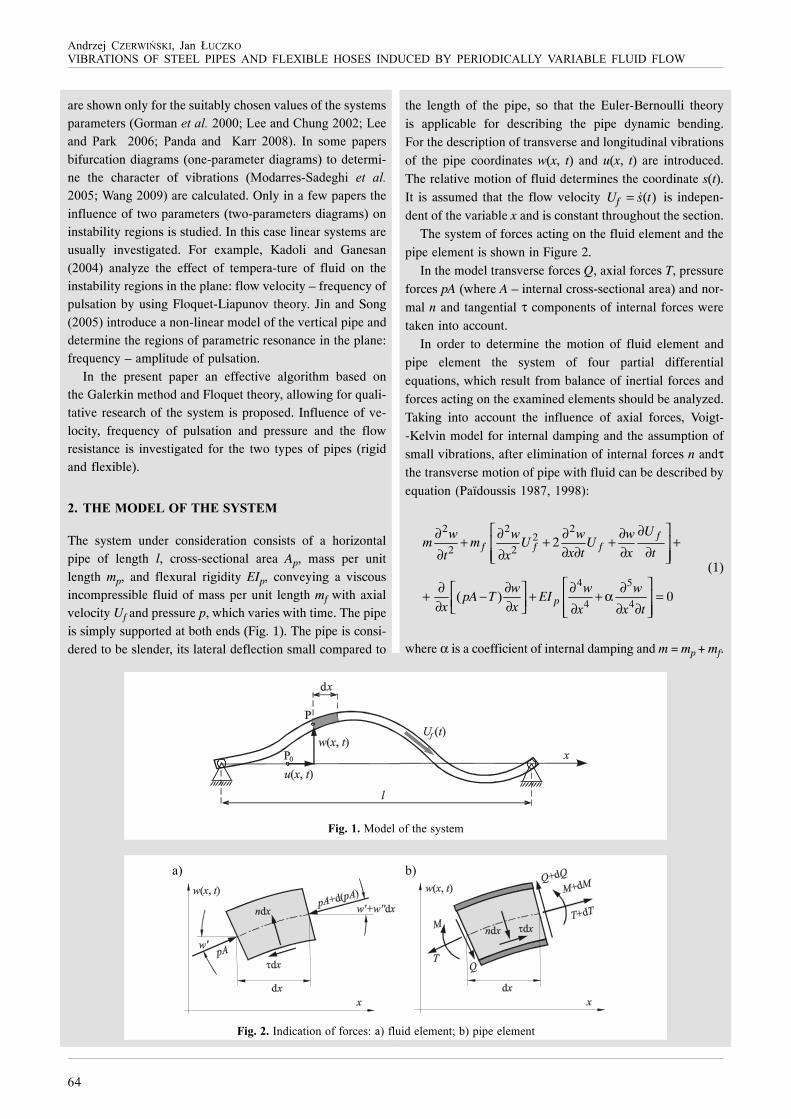
The system under consideration consists of a horizontalpipe of length l, cross-sectional area Ap, mass per unitlength mp, and flexural rigidity EIp, conveying a viscousincompressible fluid of mass per unit length mf with axialvelocity Uf and pressure p, which varies with time. The pipeis simply supported at both ends (Fig. 1). The pipe is consi-dered to be slender, its lateral deflection small compared to
the length of the pipe, so that the Euler-Bernoulli theoryis applicable for describing the pipe dynamic bending.For the description of transverse and longitudinal vibrationsof the pipe coordinates w(x, t) and u(x, t) are introduced.The relative motion of fluid determines the coordinate s(t).It is assumed that the flow velocity ( )fU s t= � is indepen-dent of the variable x and is constant throughout the section.
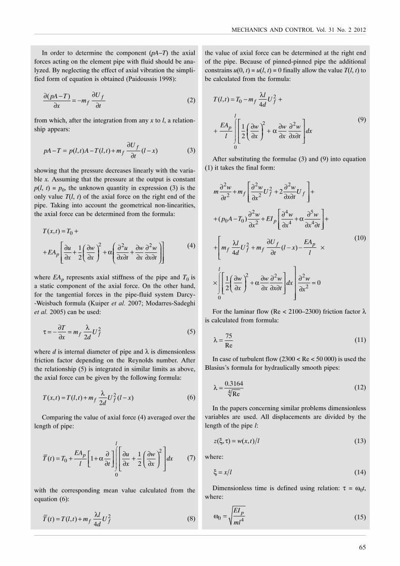
The system of forces acting on the fluid element and thepipe element is shown in Figure 2.
In the model transverse forces Q, axial forces T, pressureforces pA (where A – internal cross-sectional area) and nor-mal n and tangential τ components of internal forces weretaken into account.
In order to determine the motion of fluid element andpipe element the system of four partial differentialequations, which result from balance of inertial forces andforces acting on the examined elements should be analyzed.Taking into account the influence of axial forces, Voigt--Kelvin model for internal damping and the assumption ofsmall vibrations, after elimination of internal forces n andτthe transverse motion of pipe with fluid can be described byequation FPaïdoussis�9E7(�99EG:
2 2 22
2 2
4 5
4 4
2
( ) 0
ff f f
p
Uw w w wm m U U
x t x tt x
w w wpA T EI
x x x x t
⎡ ⎤∂∂ ∂ ∂ ∂+ + + +⎢ ⎥∂ ∂ ∂ ∂∂ ∂⎢ ⎥⎣ ⎦
⎡ ⎤∂ ∂ ∂ ∂⎡ ⎤+ − + + α =⎢ ⎥⎢ ⎥∂ ∂⎣ ⎦ ∂ ∂ ∂⎢ ⎥⎣ ⎦
(1)
where α is a coefficient of internal damping and m = mp + mf.
���������,!��%#&!"$"#!/
����������,���#����%%���!"4�G%�1�,!�!/!�#-JG0�0!!�!/!�#
�G JG

65
�������������� ������� �� ��� � ����
In order to determine the component (pA–T) the axialforces acting on the element pipe with fluid should be ana-lyzed. By neglecting the effect of axial vibration the simpli-fied form of equation is obtained F+��,�1""�"�99EG:
( ) ff
UpA Tm
x t
∂∂ − = −∂ ∂
(2)
from which, after the integration from any x to l, a relation-ship appears:
( , ) ( , ) ( )f
fU
pA T p l t A T l t m l xt
∂− = − + −
∂(3)
showing that the pressure decreases linearly with the varia-ble x. Assuming that the pressure at the output is constantp(l, t) = p0, the unknown quantity in expression (3) is theonly value T(l, t) of the axial force on the right end of thepipe. Taking into account the geometrical non-linearities,the axial force can be determined from the formula:
0
2 2 2
( , )
1
2p
T x t T
u w u w wEA
x x x t x x t
= +
⎡ ⎤⎛ ⎞∂ ∂ ∂ ∂ ∂⎛ ⎞+ ⎢ + + α + ⎥⎜ ⎟⎜ ⎟ ⎜ ⎟∂ ∂ ∂ ∂ ∂ ∂ ∂⎝ ⎠⎢ ⎥⎝ ⎠⎣ ⎦
(4)
where EAp represents axial stiffness of the pipe and T0 isa static component of the axial force. On the other hand,for the tangential forces in the pipe-fluid system Darcy--Weisbach formula ()1�0!����������7- ��,���!"I�,!'&����������DG can be used:
2
2f fT
m Ux d
∂ λτ = − =∂
(5)
where d is internal diameter of pipe and λ is dimensionlessfriction factor depending on the Reynolds number. Afterthe relationship (5) is integrated in similar limits as above,the axial force can be given by the following formula:
2( , ) ( , ) ( )2f fT x t T l t m U l x
d
λ= + − (6)
Comparing the value of axial force (4) averaged over thelength of pipe:
2
0
0
1( ) 1
2
l
pEA u wT t T dx
l t x x
⌠⎮⎮⎮⎮⌡
⎡ ⎤∂ ∂ ∂⎡ ⎤ ⎛ ⎞⎢ ⎥= + + α + ⎜ ⎟⎢ ⎥ ⎢ ⎥∂ ∂ ∂⎣ ⎦ ⎝ ⎠⎣ ⎦(7)
with the corresponding mean value calculated from theequation (6):
2( ) ( , )4f f
lT t T l t m U
d
λ= + (8)
the value of axial force can be determined at the right endof the pipe. Because of pinned-pinned pipe the additionalconstrains u(0, t) = u(l, t) = 0 finally allow the value T(l, t) tobe calculated from the formula:
20
2 2
0
( , )4
1
2
f f
l
p
lT l t T m U
d
EA w w wdx
l x x x t
⌠⎮⎮⎮⎮⌡
λ= − +
⎡ ⎤∂ ∂ ∂⎛ ⎞⎢ ⎥+ + α⎜ ⎟⎢ ⎥∂ ∂ ∂ ∂⎝ ⎠⎣ ⎦
(9)
After substituting the formulae (3) and (9) into equation(1) it takes the final form:
2 2 22
2 2
2 4 5
0 0 2 4 4
2
2 2 2
2
0
2
( )
( )4
10
2
f f f
p
f pf f f
l
w w wm m U U
x tt x
w w wp A T EI
x x x t
U EAlm U m l x
d t l
w w w wdx
x x x t x
⌠⎮⎮⎮⌡
⎡ ⎤∂ ∂ ∂+ + +⎢ ⎥∂ ∂∂ ∂⎢ ⎥⎣ ⎦
⎡ ⎤∂ ∂ ∂+ − + + α +⎢ ⎥∂ ∂ ∂ ∂⎢ ⎥⎣ ⎦
⎡ ∂λ⎢+ + − − ×∂⎢⎣
⎤⎡ ⎤ ⎥∂ ∂ ∂ ∂⎛ ⎞× ⎢ + α ⎥ =⎥⎜ ⎟∂ ∂ ∂ ∂⎝ ⎠⎢ ⎥ ∂⎥⎣ ⎦
⎥⎦
(10)
For the laminar flow (Re < 2100–2300) friction factor λis calculated from formula:
75
Reλ = (11)
In case of turbulent flow (2300 < Re < 50 000) is used theBlasius’s formula for hydraulically smooth pipes:
4
0.3164
Reλ = (12)
In the papers concerning similar problems dimensionlessvariables are used. All displacements are divided by thelength of the pipe l:
( , ) ( , )z w x t lξ τ = (13)
where:
x lξ = (14)
Dimensionless time is defined using relation: τ = ω0t,where:
0 4pEI
mlω = (15)

66
��,�3!2 �;��<�=)�( >�� ?��;)���@�� ��� �A ��� +�+� ��� A��B�@�� ��� ������� @C +����������C �����@�� A���� A��<
4 2 21 1 1 2 4 2 4
16 32 64 512( ) 0
3 15 9 225z z f z U z z U z z⎡ ⎤ ⎡ ⎤+ ζπ + π π + − β + − β + =⎢ ⎥ ⎢ ⎥⎣ ⎦ ⎣ ⎦
�
�� � � �
4 2 22 2 2 1 3 1 3
16 48 16 43216 4 (4 ) 0
3 5 9 25z z f z U z z U z z
⎡ ⎤ ⎡ ⎤+ ζπ + π π + + β − −β + =⎢ ⎥ ⎢ ⎥⎣ ⎦ ⎣ ⎦�
�� � � �
(19)
4 2 23 3 3 2 4 2 4
48 96 192 153681 9 (9 ) 0
5 7 25 49z z f z U z z U z z
⎡ ⎤ ⎡ ⎤+ ζπ + π π + + β − −β − =⎢ ⎥ ⎢ ⎥⎣ ⎦ ⎣ ⎦�
�� � � �
4 2 24 4 4 1 3 1 3
32 96 32 864256 16 (16 ) 0
15 7 225 49z z f z U z z U z z
⎡ ⎤ ⎡ ⎤+ ζπ + π π + + β + −β − =⎢ ⎥ ⎢ ⎥⎣ ⎦ ⎣ ⎦�
�� � � �
Equation (10) in dimensionless variables takes the form:
1
2 22
0
2
1 1(1 ) (1 )
2
0IV IV
z Uz
U q U z z z d
z z z
⌠⎮⎮⌡
′+ β +
⎡ ⎤⎛ ⎞⎢ ⎥′ ′ ′+ + γ + σ − + β − ξ − + ζ ξ ×⎜ ⎟⎢ ⎥⎝ ⎠ρ⎢ ⎥⎣ ⎦
′′× + + ζ =
�� �
�
�
�
(16)
where differentiation with respect to the variable τ is mar-ked by dot and differentiation with respect to the variable ξis marked by prim. The parameters appearing in equation(16) are defined by the formulae:
0 20
2 20 0
20
(Re)
4
f f p
p
f
p p
m U IU
m l A l
T l p Al lq
EI EI d l
ββ = = ζ = αω ρ =
ω
νλ= σ = γ = ν =ω
(17)
The value of coefficient γ depends by formulae (11) and(12) on the Reynolds number Re ,f fU d Ud l= ν = νβwhich depends on the dimensionless parameters ν, U and β.
�� � ����� �������������
As a first step towards solving the nonlinear partialdifferential equation (16), it is transformed into a set of se-cond-order ordinary differential equations using Galerkin’stechnique F�!! ��, �&1�' ����- <��' ���9G with thebeam eigenfunctions. For simply supported pipe the appro-ximate solution can be assumed in the following form:
1
( , ) ( ) sinN
kk
z z k=
ξ τ = τ πξ∑ (18)
Due to the influence of gyroscopic effects, in the numeri-cal calculation an even number of forms (N = 4) is included.In this case, after applying the Galerkin method and takinginto account the conditions of orthogonality of trigonome-tric functions, set of four second-order ordinary differentialequations is obtained in the form:
where:
2 1(1 )
2 NLf q U U f= − σ − + γ − β +� (20)
and:
2 2 2 21 2 3 42
1 1 2 2 3 3 4 4
1[ 4 9 16
4
2 ( 4 9 16 )]
NLf z z z z
z z z z z z z z
= + + + +ρ
+ ζ + + +� � � �
(21)
Equations (19) include the influence of gyroscopic ef-fects (terms with parameter βU), internal damping (parame-ter ζ) and geometric non-linearities (term fNL). These arenonlinear parametrical equations due to the dependence ofthe dimensionless flow velocity on the time. The velocity offlow is assumed to be harmonically varying:
0 (1 sin )UU U A= + ωτ (22)
where U0 is the mean velocity and AU is amplitude of pulsa-tion and ω is excitation frequency.
The set of nonlinear equations (19) can be solved byusing the methods of numerical integration, such as theRunge-Kutta methods. After using the relation (18) the di-splacements and velocities at any point of the pipe can alsobe determined.
Estimation of the regions of parametric resonance inthe plane of the parameters is associated with multiplesolving the equations (19) for different values of this pa-rameters. This fact requires a relatively long time of cal-culations.
In order to estimate the range of parametric resonancethe linear system (equations (19) for fNL = 0) can be ana-lyzed. In this case a very effective way to study the stabilityis the method based on the Floquet theory. In order to inve-stigate the stability of solutions, the eigenvalues of the mo-nodromy matrix (Floquet multipliers) are used. The mainadvantage of this method is a relatively short time of nume-rical calculations due to the fact, that to determine the mo-nodromy matrix the requirement is integration of differen-tial equations (19) in one period of excitation only.
67
�������������� ������� �� ��� � ����
�� ��������� ��������
The numerical calculations were performed for two types ofhydraulic line: steel pipe (Young’s modulus E = 2.1×10¹¹ Pa,mass per unit length mp = 0.222 kg/m) with outer diameter10 mm and wall thickness 1mm and hydraulic rubber hose(E = 3×10⁸ Pa, mp = 0.25 kg/m) with outer diameter 15.4 mmand wall thickness 3.7 mm. Both of them have a length ofl = 1 m. Mass of oil per unit length is mf = 0.0503 kg/m. Theinfluence of the constant component of axial force (q = 0)was omitted. This data was used to calculate ranges of va-riation of dimensionless parameters (seen in Table 1).
�������
���1!"�%,�/!�"����!""0���/!#!�"�%�� !"#�'�#!,&$,��1������!"
In the tested system the flow velocity is harmonicallyvarying according to the relation (22). The influence of theparameters characterizing the excitation, such as mean flowvelocity U0, pulsation amplitude AU and frequency ω
as well as the parameters of the hydraulic system such aspressure σ at the end of the line and kinematic viscosity ν,was determined.
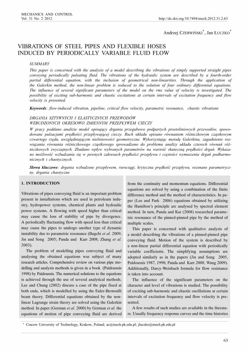
Figure 3 illustrates the effect of the parameters 0U� and ω�on the rms value of the vibration velocity (in one-fourth thelength of the pipe). The figure shows boundaries of unstableregions determined from the condition, that the value of themaximum Floquet multiplier is greater than unity. In addi-tion, the graphs the curves defining the relationship betwe-en the frequency of excitation and the natural frequency, forwhich in theory should occurs the parametric resonance arealso shown.
Vibrations induced by fluid flow occur mainly for thevelocity greater than the critical velocity. Below the criticalvelocity the vibration are generated only in the ranges ofparametric resonance. This phenomenon is more visible inthe case of the steel pipe. In Figure 3d-f we can see clearlythe first three areas of the parametric resonance. The incre-ase of viscosity (flow resistance) shifts the range of excita-tion of vibrations to the lower flow rate. For the flexiblehose for viscosity equal ν = 3⋅10–4 (Fig. 3c) vibrations occurin the whole range of flow rates.
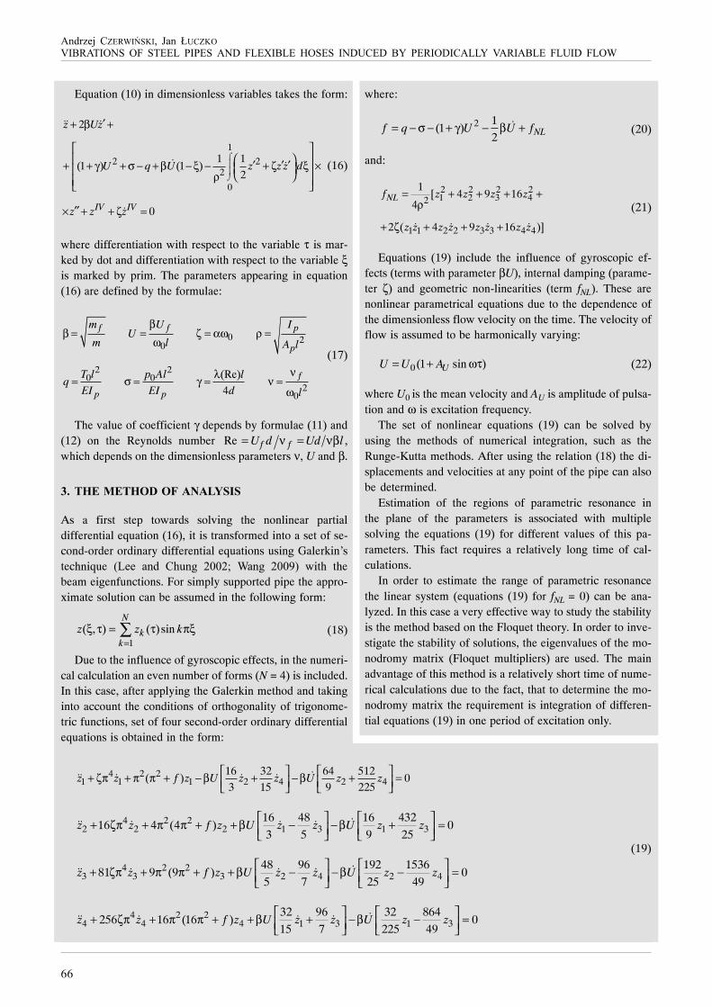
Figures 4 and 5 shows the influence of the parameters 0U�
and σ� on the rms value of the vibration velocity. The solidline shows boundaries of unstable regions. The dashedline shows the relationship between the parameters 0U�
and σ� for which relationship ω� = 2 (ω = 2ωn0) occurs, thatis a condition for principal parametric resonance. In thegraph time histories and spectra of vibration velocity
14( , )zV z= τ� for selected values of the parameters 0U� and σ�
are shown.
������� &!!%%!�#�%#&!0���/!#!�" 0U� ��,�ω� ���#&!�/" ��1!�%#&! �J��#��� !����#$F 0σ =� (��K���DG%��%�!6�J�!&�"!4�GνK�-JGν K�L��MD-�Gν K�L��M8��,%��"#!!�0�0!4,GνK�-!GνK�L��M:-%GνK�L��MD
Parameter Steel pipe Rubber hose
Pulsation frequency ω 1–30 1–30
Flow velocity U0 0–1.5π 0–1.5π
Coefficient β 0.43 0.41
Damping coefficient ζ 0.002 0.02
Radius of gyration ρ 3.2×10⁻³ 4.4×10⁻³
Pressure σ 0–10 0–10
Kinematics viscosity ν 3×10⁻⁶–15×10–6 3×10⁻⁵–15×10–5

68
��,�3!2 �;��<�=)�( >�� ?��;)���@�� ��� �A ��� +�+� ��� A��B�@�� ��� ������� @C +����������C �����@�� A���� A��<
�������� &!��%�1!��!�%#&!0���/!#!�" 0U� ��,� σ� ���#&!�/" ��1!�%#&! �J��#��� !����#$�%#&!�1JJ!�&�"!�##&!�!�'&#ξ�K¼%��ω� K�(���K���D(νK�L��
M:
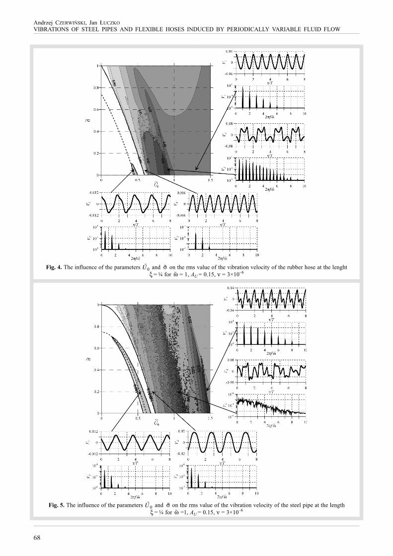
����� �� &!��%�1!��!�%#&!0���/!#!�" 0U� ��,� σ� ��#&!�/" ��1!�%#&! �J��#��� !����#$�%#&!"#!!�0�0!�##&!�!�'#&ξ�K¼ %��ω� K�(���K���D(νK�L��
M:

69
�������������� ������� �� ��� � ����
By analyzing the results, it can be seen that the increaseof pressure causes the decrease of flow velocity at which thevibration of the pipe are induced. The vibrations are genera-ted in a relatively narrow region of parametric resonance,which was calculated based on the analysis of linear system.The observation of the time histories and the spectraof vibrations for the sub-critical velocity range confirmsthe phenomenon of parametric resonance in the system.The frequency of the pipe is equal to half of the excitationfrequency. The vibration signal is polyharmonic. The spec-trum consists only the odd harmonics.
The parametric resonance is more visible in the case ofthe steel pipe (Fig. 5). In the range of the velocity a fewpercent higher then critical velocity, the nature of vibrationsdepends on the type of hydraulic line. For the steel pipeperiod of vibration is twice as high as period of excitation(a typical feature of parametric oscillation), in the case ofthe flexible hose (Fig. 4) the frequency of oscillation isequal to the frequency of flow pulsation. For the steel pipein the area of supercritical flow velocity, can be seen tworegions of increased levels of vibrations. In the first regionthe vibrations are non-periodic (chaotic), in the secondregion the vibrations are periodic (with a frequency ofextortion). In the case of the rubber hose with an increaseof flow velocity is observed one maximum of vibration.In this area polyharmonic vibrations of frequency are equalto half of the excitation frequency. For higher flow velocitythe hose vibrates with frequency of flow pulsation.
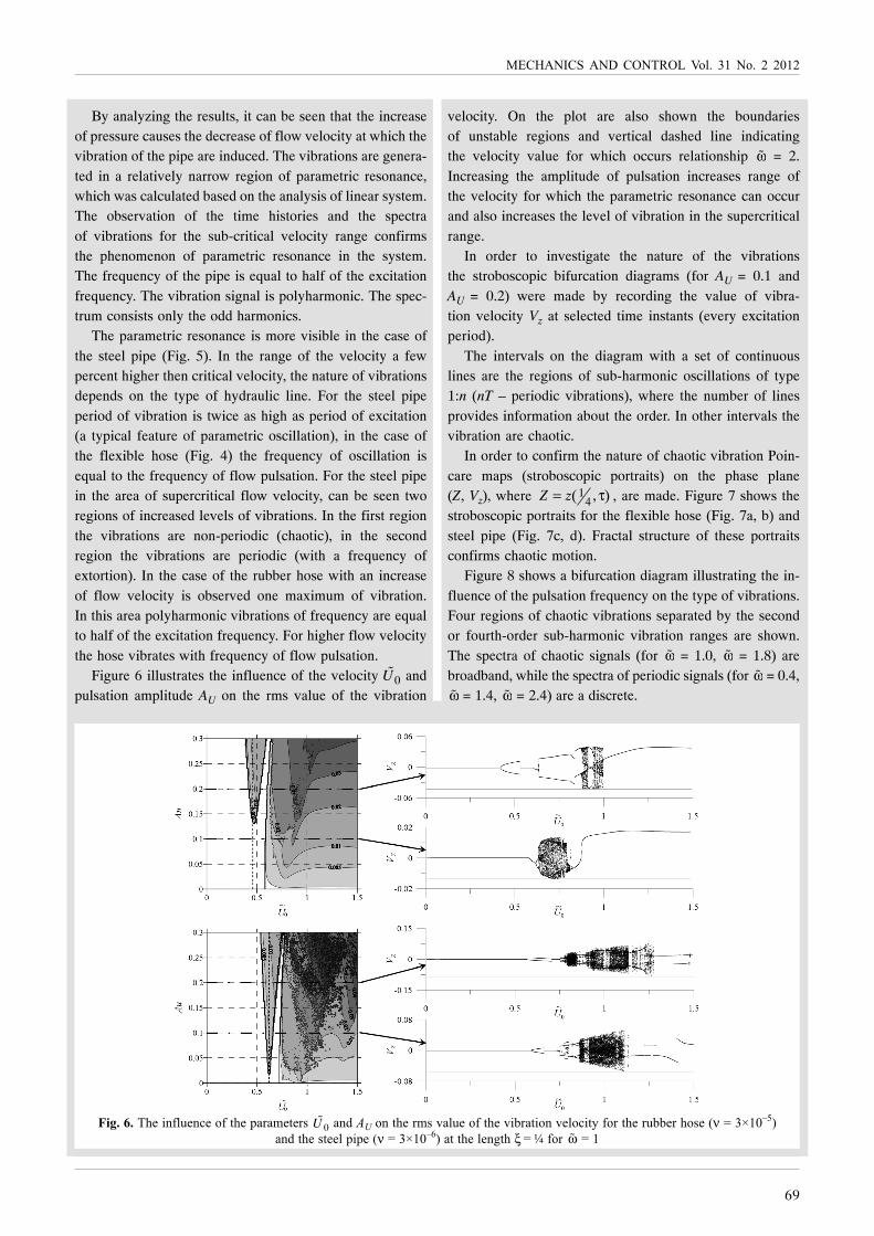
Figure 6 illustrates the influence of the velocity 0U� andpulsation amplitude AU on the rms value of the vibration
velocity. On the plot are also shown the boundariesof unstable regions and vertical dashed line indicatingthe velocity value for which occurs relationship ω� = 2.Increasing the amplitude of pulsation increases range ofthe velocity for which the parametric resonance can occurand also increases the level of vibration in the supercriticalrange.
In order to investigate the nature of the vibrationsthe stroboscopic bifurcation diagrams (for AU = 0.1 andAU = 0.2) were made by recording the value of vibra-tion velocity Vz at selected time instants (every excitationperiod).
The intervals on the diagram with a set of continuouslines are the regions of sub-harmonic oscillations of type1:n (nT – periodic vibrations), where the number of linesprovides information about the order. In other intervals thevibration are chaotic.
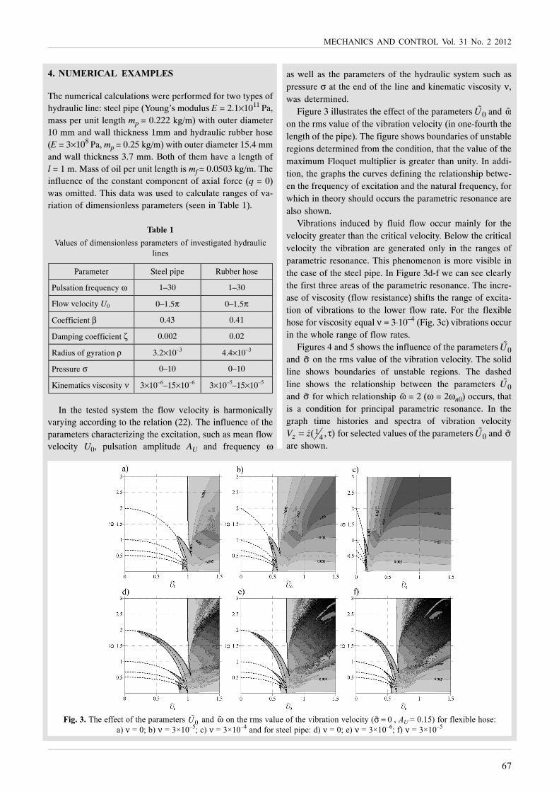
In order to confirm the nature of chaotic vibration Poin-care maps (stroboscopic portraits) on the phase plane(Z, Vz), where 1
4( , )Z z= τ , are made. Figure 7 shows thestroboscopic portraits for the flexible hose (Fig. 7a, b) andsteel pipe (Fig. 7c, d). Fractal structure of these portraitsconfirms chaotic motion.
Figure 8 shows a bifurcation diagram illustrating the in-fluence of the pulsation frequency on the type of vibrations.Four regions of chaotic vibrations separated by the secondor fourth-order sub-harmonic vibration ranges are shown.The spectra of chaotic signals (for ω� = 1.0, ω� = 1.8) arebroadband, while the spectra of periodic signals (for ω� = 0.4,ω� = 1.4, ω� = 2.4) are a discrete.
�����!�� &!��%�1!��!�%#&!0���/!#!�" 0U� ��,������#&!�/" ��1!�%#&! �J��#��� !����#$%��#&!�1JJ!�&�"!FνK�L��MDG��,#&!"#!!�0�0!FνK�L��M:G�##&!�!�'#&ξ�K¼ %��ω� K�
70
��,�3!2 �;��<�=)�( >�� ?��;)���@�� ��� �A ��� +�+� ��� A��B�@�� ��� ������� @C +����������C �����@�� A���� A��<
�����"�� &!+������!/�0"Fω� K�G%��#&!�1JJ!�&�"!4�G���K���( 0U� K��7D-JG���K���( 0U� K��9��,#&!"#!!�0�0!4�G���K���( 0U� K��E-,G���K���( 0U� K�
�����#�� &!J�%1���#���,��'��/��,#&!"0!�#���% �J��#��� !����#$�#"!�!�#���0���#"�%,��'��/F#&!�1JJ!�&�"!4���K���( 0U� K��9G
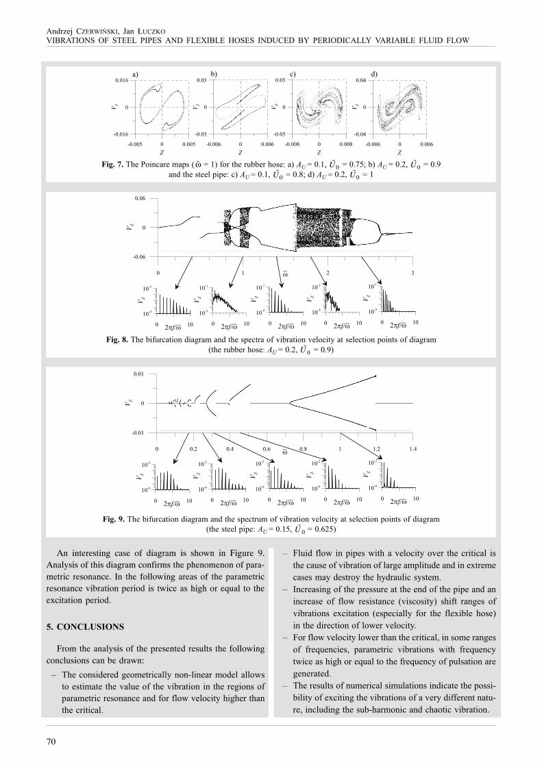
An interesting case of diagram is shown in Figure 9.Analysis of this diagram confirms the phenomenon of para-metric resonance. In the following areas of the parametricresonance vibration period is twice as high or equal to theexcitation period.
� ����������
From the analysis of the presented results the followingconclusions can be drawn:
M &!���"�,!�!,'!�/!#������$���I���!��/�,!������"#�!"#�/�#!#&! ��1!�%#&! �J��#�����#&!�!'���"�%0���/!#����!"�����!��,%��%��� !����#$&�'&!�#&��#&!���#�����
M A�1�, %��� ��0�0!"��#&� !����#$� !� #&!���#���� �"#&!��1"!�% �J��#����%���'!�/0��#1,!��,��!6#�!/!��"!"/�$,!"#��$#&!&$,��1���"$"#!/�
M ����!�"��'�%#&!0�!""1�!�##&!!�,�%#&!0�0!��,������!�"! �% %��� �!"�"#���! F �"��"�#$G "&�%# ���'!" �% �J��#���" !6��#�#��� F!"0!�����$ %�� #&! %�!6�J�! &�"!G��#&!,��!�#����%���!� !����#$�
M A��%��� !����#$���!�#&��#&!���#����(��"�/!���'!"�% %�!N1!���!"( 0���/!#��� �J��#���" ��#& %�!N1!��$#���!�"&�'&��!N1��#�#&!%�!N1!��$�%01�"�#�����!'!�!��#!,�
M &!�!"1�#"�%�1/!�����"�/1��#���"��,���#!#&!0�""�IJ���#$�%!6��#��'#&! �J��#���"�%� !�$,�%%!�!�#��#1I�!(����1,��'#&!"1JI&��/������,�&��#�� �J��#����
�����$� &!J�%1���#���,��'��/��,#&!"0!�#�1/�% �J��#��� !����#$�#"!�!�#���0���#"�%,��'��/F#&!"#!!�0�0!4���K���D( 0U� K��:�DG
71
�������������� ������� �� ��� � ����
M &! �!"1�#" �% �1/!����� ����$"�" ���J! #&!J�"�" %��"!�!�#����%#&!&$,��1���"$"#!/��#&!0����!,!60!��I/!�#�
��%�&�'(�)
@�'�&�)�(H10#��)�()1"&�����(�$!�'����H���(���9(.% �������������� ��� �������� ������������ ���� ����� ������������ �� ��� ���������� �������� ��( >�1���� �% �1�, ��, ��J��#���( ��E(00�88�M8DD�
H��/����H�(�!!"!>���(;&��'C���(����(@���������������%���� ����������������� �����������������(>�1�����%�1�,��,��J��I#���(���(�(00��79M�9��
>�� >���( ��' ;�C�( ���D( 0��������� ����������� ��� �� ������ ����������� �������� ����( >�1���� �% A�1�," ��, #�1�#1�!"( ��(00�7:�M7E��
)�,�����(H��!"����(���8(0��������������������������� ��������� �������������������� �����������������������(��/0�"�#!#�1�#1I�!"(:D(00��9�M8�8
)1�0!�H���(�!#��*��!����(@�##2!">���(���7(��������� ��������������� ���� ���� ��� ��������� ��� ��� ������� �������� ��� �� ��� ������� �� ��������� ����( >�1���� �% A�1�," ��, #�1�#1�!"( ��(00�8�9M88D�
�!!���(�&1�'>�(����((������ ���������������������������������������������� ����������� ����( >�1�����%�1�,��,��J��#���(�D8(�(00����M��D�
�!!��(+��*>�(���:(� ����������������������������������������� � ����������������������������������(>�1�����%A�1�,"��,#�1�#1I�!"(��(00��7�M�9��
��,���!"I�,!'&� C�( +�O,�1""�" ��+�( !/�!� ��( ���D( �� �������������� ��������%���������������� ���%���������������7������ ����%������(>�1�����%A�1�,"��,#�1�#1�!"(��(00�:�9M:�7�
Païdoussis M.P.,�9E7(A��� ���������������������������������������(�00��!,�!�&����"(8�(�:�I�7D�
Païdoussis, M.P., �99E(A��� ���������� )����������&� �������� ���������������%���A���( ����(���,!/��+�!""(���,���
+��,� ����( )�� ����( ���E( (�������� �������� ��� �� �� ��� ������ �������� ����� ��� ���������"� ��� ��� ������������ �������� ����������( >�1���� �% �1�, ��, ��J��#���( ��9(00��7DM8�:�
<��' ��( ���9( �� ������� ������ ��� ��� ��� ������ �������� ��� �� ���� ������ ��� ��������� �������� ����( ��#!���#����� >�1���� �%���I���!���!�&����"(88(00���DM����
;&��'C���(�!!"!>���(H��/����H�(����(����% ������������������������������� ���������������������������������������������������������7����������%��������������(>�1�����%�1�,��,��J��#���(�::(00��DDM�:7�
64
��,�3!2 �;��<�=)�( >�� ?��;)���@�� ��� �A ��� +�+� ��� A��B�@�� ��� ������� @C +����������C �����@�� A���� A��<
are shown only for the suitably chosen values of the systemsparameters (H��/�������������-�!!��,�&1�'����- �!!��, +��* ���:- +��,� ��, )��� ���EG. In some papersbifurcation diagrams (one-parameter diagrams) to determi-ne the character of vibrations (��,���!"I�,!'&� ��� ������D; <��'���9G are calculated. Only in a few papers theinfluence of two parameters (two-parameters diagrams) oninstability regions is studied. In this case linear systems areusually investigated. For example, Kadoli and GanesanF���8G analyze the effect of tempera-ture of fluid on theinstability regions in the plane: flow velocity – frequency ofpulsation by using Floquet-Liapunov theory. Jin and SongF���DG introduce a non-linear model of the vertical pipe anddetermine the regions of parametric resonance in the plane:frequency – amplitude of pulsation.
In the present paper an effective algorithm based onthe Galerkin method and Floquet theory, allowing for quali-tative research of the system is proposed. Influence of ve-locity, frequency of pulsation and pressure and the flowresistance is investigated for the two types of pipes (rigidand flexible).
�� � ����������� ��������
The system under consideration consists of a horizontalpipe of length l, cross-sectional area Ap, mass per unitlength mp, and flexural rigidity EIp, conveying a viscousincompressible fluid of mass per unit length mf with axialvelocity Uf and pressure p, which varies with time. The pipeis simply supported at both ends (Fig. 1). The pipe is consi-dered to be slender, its lateral deflection small compared to
the length of the pipe, so that the Euler-Bernoulli theoryis applicable for describing the pipe dynamic bending.For the description of transverse and longitudinal vibrationsof the pipe coordinates w(x, t) and u(x, t) are introduced.The relative motion of fluid determines the coordinate s(t).It is assumed that the flow velocity ( )fU s t= � is indepen-dent of the variable x and is constant throughout the section.
The system of forces acting on the fluid element and thepipe element is shown in Figure 2.
In the model transverse forces Q, axial forces T, pressureforces pA (where A – internal cross-sectional area) and nor-mal n and tangential τ components of internal forces weretaken into account.
In order to determine the motion of fluid element andpipe element the system of four partial differentialequations, which result from balance of inertial forces andforces acting on the examined elements should be analyzed.Taking into account the influence of axial forces, Voigt--Kelvin model for internal damping and the assumption ofsmall vibrations, after elimination of internal forces n andτthe transverse motion of pipe with fluid can be described byequation FPaïdoussis�9E7(�99EG:
2 2 22
2 2
4 5
4 4
2
( ) 0
ff f f
p
Uw w w wm m U U
x t x tt x
w w wpA T EI
x x x x t
⎡ ⎤∂∂ ∂ ∂ ∂+ + + +⎢ ⎥∂ ∂ ∂ ∂∂ ∂⎢ ⎥⎣ ⎦
⎡ ⎤∂ ∂ ∂ ∂⎡ ⎤+ − + + α =⎢ ⎥⎢ ⎥∂ ∂⎣ ⎦ ∂ ∂ ∂⎢ ⎥⎣ ⎦
(1)
where α is a coefficient of internal damping and m = mp + mf.
���������,!��%#&!"$"#!/
����������,���#����%%���!"4�G%�1�,!�!/!�#-JG0�0!!�!/!�#
�G JG
65
�������������� ������� �� ��� � ����
In order to determine the component (pA–T) the axialforces acting on the element pipe with fluid should be ana-lyzed. By neglecting the effect of axial vibration the simpli-fied form of equation is obtained F+��,�1""�"�99EG:
( ) ff
UpA Tm
x t
∂∂ − = −∂ ∂
(2)
from which, after the integration from any x to l, a relation-ship appears:
( , ) ( , ) ( )f
fU
pA T p l t A T l t m l xt
∂− = − + −
∂(3)
showing that the pressure decreases linearly with the varia-ble x. Assuming that the pressure at the output is constantp(l, t) = p0, the unknown quantity in expression (3) is theonly value T(l, t) of the axial force on the right end of thepipe. Taking into account the geometrical non-linearities,the axial force can be determined from the formula:
0
2 2 2
( , )
1
2p
T x t T
u w u w wEA
x x x t x x t
= +
⎡ ⎤⎛ ⎞∂ ∂ ∂ ∂ ∂⎛ ⎞+ ⎢ + + α + ⎥⎜ ⎟⎜ ⎟ ⎜ ⎟∂ ∂ ∂ ∂ ∂ ∂ ∂⎝ ⎠⎢ ⎥⎝ ⎠⎣ ⎦
(4)
where EAp represents axial stiffness of the pipe and T0 isa static component of the axial force. On the other hand,for the tangential forces in the pipe-fluid system Darcy--Weisbach formula ()1�0!����������7- ��,���!"I�,!'&����������DG can be used:
2
2f fT
m Ux d
∂ λτ = − =∂
(5)
where d is internal diameter of pipe and λ is dimensionlessfriction factor depending on the Reynolds number. Afterthe relationship (5) is integrated in similar limits as above,the axial force can be given by the following formula:
2( , ) ( , ) ( )2f fT x t T l t m U l x
d
λ= + − (6)
Comparing the value of axial force (4) averaged over thelength of pipe:
2
0
0
1( ) 1
2
l
pEA u wT t T dx
l t x x
⌠⎮⎮⎮⎮⌡
⎡ ⎤∂ ∂ ∂⎡ ⎤ ⎛ ⎞⎢ ⎥= + + α + ⎜ ⎟⎢ ⎥ ⎢ ⎥∂ ∂ ∂⎣ ⎦ ⎝ ⎠⎣ ⎦(7)
with the corresponding mean value calculated from theequation (6):
2( ) ( , )4f f
lT t T l t m U
d
λ= + (8)
the value of axial force can be determined at the right endof the pipe. Because of pinned-pinned pipe the additionalconstrains u(0, t) = u(l, t) = 0 finally allow the value T(l, t) tobe calculated from the formula:
20
2 2
0
( , )4
1
2
f f
l
p
lT l t T m U
d
EA w w wdx
l x x x t
⌠⎮⎮⎮⎮⌡
λ= − +
⎡ ⎤∂ ∂ ∂⎛ ⎞⎢ ⎥+ + α⎜ ⎟⎢ ⎥∂ ∂ ∂ ∂⎝ ⎠⎣ ⎦
(9)
After substituting the formulae (3) and (9) into equation(1) it takes the final form:
2 2 22
2 2
2 4 5
0 0 2 4 4
2
2 2 2
2
0
2
( )
( )4
10
2
f f f
p
f pf f f
l
w w wm m U U
x tt x
w w wp A T EI
x x x t
U EAlm U m l x
d t l
w w w wdx
x x x t x
⌠⎮⎮⎮⌡
⎡ ⎤∂ ∂ ∂+ + +⎢ ⎥∂ ∂∂ ∂⎢ ⎥⎣ ⎦
⎡ ⎤∂ ∂ ∂+ − + + α +⎢ ⎥∂ ∂ ∂ ∂⎢ ⎥⎣ ⎦
⎡ ∂λ⎢+ + − − ×∂⎢⎣
⎤⎡ ⎤ ⎥∂ ∂ ∂ ∂⎛ ⎞× ⎢ + α ⎥ =⎥⎜ ⎟∂ ∂ ∂ ∂⎝ ⎠⎢ ⎥ ∂⎥⎣ ⎦
⎥⎦
(10)
For the laminar flow (Re < 2100–2300) friction factor λis calculated from formula:
75
Reλ = (11)
In case of turbulent flow (2300 < Re < 50 000) is used theBlasius’s formula for hydraulically smooth pipes:
4
0.3164
Reλ = (12)
In the papers concerning similar problems dimensionlessvariables are used. All displacements are divided by thelength of the pipe l:
( , ) ( , )z w x t lξ τ = (13)
where:
x lξ = (14)
Dimensionless time is defined using relation: τ = ω0t,where:
0 4pEI
mlω = (15)
66
��,�3!2 �;��<�=)�( >�� ?��;)���@�� ��� �A ��� +�+� ��� A��B�@�� ��� ������� @C +����������C �����@�� A���� A��<
4 2 21 1 1 2 4 2 4
16 32 64 512( ) 0
3 15 9 225z z f z U z z U z z⎡ ⎤ ⎡ ⎤+ ζπ + π π + − β + − β + =⎢ ⎥ ⎢ ⎥⎣ ⎦ ⎣ ⎦
�
�� � � �
4 2 22 2 2 1 3 1 3
16 48 16 43216 4 (4 ) 0
3 5 9 25z z f z U z z U z z
⎡ ⎤ ⎡ ⎤+ ζπ + π π + + β − −β + =⎢ ⎥ ⎢ ⎥⎣ ⎦ ⎣ ⎦�
�� � � �
(19)
4 2 23 3 3 2 4 2 4
48 96 192 153681 9 (9 ) 0
5 7 25 49z z f z U z z U z z
⎡ ⎤ ⎡ ⎤+ ζπ + π π + + β − −β − =⎢ ⎥ ⎢ ⎥⎣ ⎦ ⎣ ⎦�
�� � � �
4 2 24 4 4 1 3 1 3
32 96 32 864256 16 (16 ) 0
15 7 225 49z z f z U z z U z z
⎡ ⎤ ⎡ ⎤+ ζπ + π π + + β + −β − =⎢ ⎥ ⎢ ⎥⎣ ⎦ ⎣ ⎦�
�� � � �
Equation (10) in dimensionless variables takes the form:
1
2 22
0
2
1 1(1 ) (1 )
2
0IV IV
z Uz
U q U z z z d
z z z
⌠⎮⎮⌡
′+ β +
⎡ ⎤⎛ ⎞⎢ ⎥′ ′ ′+ + γ + σ − + β − ξ − + ζ ξ ×⎜ ⎟⎢ ⎥⎝ ⎠ρ⎢ ⎥⎣ ⎦
′′× + + ζ =
�� �
�
�
�
(16)
where differentiation with respect to the variable τ is mar-ked by dot and differentiation with respect to the variable ξis marked by prim. The parameters appearing in equation(16) are defined by the formulae:
0 20
2 20 0
20
(Re)
4
f f p
p
f
p p
m U IU
m l A l
T l p Al lq
EI EI d l
ββ = = ζ = αω ρ =
ω
νλ= σ = γ = ν =ω
(17)
The value of coefficient γ depends by formulae (11) and(12) on the Reynolds number Re ,f fU d Ud l= ν = νβwhich depends on the dimensionless parameters ν, U and β.
�� � ����� �������������
As a first step towards solving the nonlinear partialdifferential equation (16), it is transformed into a set of se-cond-order ordinary differential equations using Galerkin’stechnique F�!! ��, �&1�' ����- <��' ���9G with thebeam eigenfunctions. For simply supported pipe the appro-ximate solution can be assumed in the following form:
1
( , ) ( ) sinN
kk
z z k=
ξ τ = τ πξ∑ (18)
Due to the influence of gyroscopic effects, in the numeri-cal calculation an even number of forms (N = 4) is included.In this case, after applying the Galerkin method and takinginto account the conditions of orthogonality of trigonome-tric functions, set of four second-order ordinary differentialequations is obtained in the form:
where:
2 1(1 )
2 NLf q U U f= − σ − + γ − β +� (20)
and:
2 2 2 21 2 3 42
1 1 2 2 3 3 4 4
1[ 4 9 16
4
2 ( 4 9 16 )]
NLf z z z z
z z z z z z z z
= + + + +ρ
+ ζ + + +� � � �
(21)
Equations (19) include the influence of gyroscopic ef-fects (terms with parameter βU), internal damping (parame-ter ζ) and geometric non-linearities (term fNL). These arenonlinear parametrical equations due to the dependence ofthe dimensionless flow velocity on the time. The velocity offlow is assumed to be harmonically varying:
0 (1 sin )UU U A= + ωτ (22)
where U0 is the mean velocity and AU is amplitude of pulsa-tion and ω is excitation frequency.
The set of nonlinear equations (19) can be solved byusing the methods of numerical integration, such as theRunge-Kutta methods. After using the relation (18) the di-splacements and velocities at any point of the pipe can alsobe determined.
Estimation of the regions of parametric resonance inthe plane of the parameters is associated with multiplesolving the equations (19) for different values of this pa-rameters. This fact requires a relatively long time of cal-culations.
In order to estimate the range of parametric resonancethe linear system (equations (19) for fNL = 0) can be ana-lyzed. In this case a very effective way to study the stabilityis the method based on the Floquet theory. In order to inve-stigate the stability of solutions, the eigenvalues of the mo-nodromy matrix (Floquet multipliers) are used. The mainadvantage of this method is a relatively short time of nume-rical calculations due to the fact, that to determine the mo-nodromy matrix the requirement is integration of differen-tial equations (19) in one period of excitation only.

67
�������������� ������� �� ��� � ����
�� ��������� ��������
The numerical calculations were performed for two types ofhydraulic line: steel pipe (Young’s modulus E = 2.1×10¹¹ Pa,mass per unit length mp = 0.222 kg/m) with outer diameter10 mm and wall thickness 1mm and hydraulic rubber hose(E = 3×10⁸ Pa, mp = 0.25 kg/m) with outer diameter 15.4 mmand wall thickness 3.7 mm. Both of them have a length ofl = 1 m. Mass of oil per unit length is mf = 0.0503 kg/m. Theinfluence of the constant component of axial force (q = 0)was omitted. This data was used to calculate ranges of va-riation of dimensionless parameters (seen in Table 1).
�������
���1!"�%,�/!�"����!""0���/!#!�"�%�� !"#�'�#!,&$,��1������!"
In the tested system the flow velocity is harmonicallyvarying according to the relation (22). The influence of theparameters characterizing the excitation, such as mean flowvelocity U0, pulsation amplitude AU and frequency ω
as well as the parameters of the hydraulic system such aspressure σ at the end of the line and kinematic viscosity ν,was determined.
Figure 3 illustrates the effect of the parameters 0U� and ω�on the rms value of the vibration velocity (in one-fourth thelength of the pipe). The figure shows boundaries of unstableregions determined from the condition, that the value of themaximum Floquet multiplier is greater than unity. In addi-tion, the graphs the curves defining the relationship betwe-en the frequency of excitation and the natural frequency, forwhich in theory should occurs the parametric resonance arealso shown.
Vibrations induced by fluid flow occur mainly for thevelocity greater than the critical velocity. Below the criticalvelocity the vibration are generated only in the ranges ofparametric resonance. This phenomenon is more visible inthe case of the steel pipe. In Figure 3d-f we can see clearlythe first three areas of the parametric resonance. The incre-ase of viscosity (flow resistance) shifts the range of excita-tion of vibrations to the lower flow rate. For the flexiblehose for viscosity equal ν = 3⋅10–4 (Fig. 3c) vibrations occurin the whole range of flow rates.
Figures 4 and 5 shows the influence of the parameters 0U�
and σ� on the rms value of the vibration velocity. The solidline shows boundaries of unstable regions. The dashedline shows the relationship between the parameters 0U�
and σ� for which relationship ω� = 2 (ω = 2ωn0) occurs, thatis a condition for principal parametric resonance. In thegraph time histories and spectra of vibration velocity
14( , )zV z= τ� for selected values of the parameters 0U� and σ�
are shown.
������� &!!%%!�#�%#&!0���/!#!�" 0U� ��,�ω� ���#&!�/" ��1!�%#&! �J��#��� !����#$F 0σ =� (��K���DG%��%�!6�J�!&�"!4�GνK�-JGν K�L��MD-�Gν K�L��M8��,%��"#!!�0�0!4,GνK�-!GνK�L��M:-%GνK�L��MD
Parameter Steel pipe Rubber hose
Pulsation frequency ω 1–30 1–30
Flow velocity U0 0–1.5π 0–1.5π
Coefficient β 0.43 0.41
Damping coefficient ζ 0.002 0.02
Radius of gyration ρ 3.2×10⁻³ 4.4×10⁻³
Pressure σ 0–10 0–10
Kinematics viscosity ν 3×10⁻⁶–15×10–6 3×10⁻⁵–15×10–5
68
��,�3!2 �;��<�=)�( >�� ?��;)���@�� ��� �A ��� +�+� ��� A��B�@�� ��� ������� @C +����������C �����@�� A���� A��<
�������� &!��%�1!��!�%#&!0���/!#!�" 0U� ��,� σ� ���#&!�/" ��1!�%#&! �J��#��� !����#$�%#&!�1JJ!�&�"!�##&!�!�'&#ξ�K¼%��ω� K�(���K���D(νK�L��
M:
����� �� &!��%�1!��!�%#&!0���/!#!�" 0U� ��,� σ� ��#&!�/" ��1!�%#&! �J��#��� !����#$�%#&!"#!!�0�0!�##&!�!�'#&ξ�K¼ %��ω� K�(���K���D(νK�L��
M:
69
�������������� ������� �� ��� � ����
By analyzing the results, it can be seen that the increaseof pressure causes the decrease of flow velocity at which thevibration of the pipe are induced. The vibrations are genera-ted in a relatively narrow region of parametric resonance,which was calculated based on the analysis of linear system.The observation of the time histories and the spectraof vibrations for the sub-critical velocity range confirmsthe phenomenon of parametric resonance in the system.The frequency of the pipe is equal to half of the excitationfrequency. The vibration signal is polyharmonic. The spec-trum consists only the odd harmonics.
The parametric resonance is more visible in the case ofthe steel pipe (Fig. 5). In the range of the velocity a fewpercent higher then critical velocity, the nature of vibrationsdepends on the type of hydraulic line. For the steel pipeperiod of vibration is twice as high as period of excitation(a typical feature of parametric oscillation), in the case ofthe flexible hose (Fig. 4) the frequency of oscillation isequal to the frequency of flow pulsation. For the steel pipein the area of supercritical flow velocity, can be seen tworegions of increased levels of vibrations. In the first regionthe vibrations are non-periodic (chaotic), in the secondregion the vibrations are periodic (with a frequency ofextortion). In the case of the rubber hose with an increaseof flow velocity is observed one maximum of vibration.In this area polyharmonic vibrations of frequency are equalto half of the excitation frequency. For higher flow velocitythe hose vibrates with frequency of flow pulsation.
Figure 6 illustrates the influence of the velocity 0U� andpulsation amplitude AU on the rms value of the vibration
velocity. On the plot are also shown the boundariesof unstable regions and vertical dashed line indicatingthe velocity value for which occurs relationship ω� = 2.Increasing the amplitude of pulsation increases range ofthe velocity for which the parametric resonance can occurand also increases the level of vibration in the supercriticalrange.
In order to investigate the nature of the vibrationsthe stroboscopic bifurcation diagrams (for AU = 0.1 andAU = 0.2) were made by recording the value of vibra-tion velocity Vz at selected time instants (every excitationperiod).
The intervals on the diagram with a set of continuouslines are the regions of sub-harmonic oscillations of type1:n (nT – periodic vibrations), where the number of linesprovides information about the order. In other intervals thevibration are chaotic.
In order to confirm the nature of chaotic vibration Poin-care maps (stroboscopic portraits) on the phase plane(Z, Vz), where 1
4( , )Z z= τ , are made. Figure 7 shows thestroboscopic portraits for the flexible hose (Fig. 7a, b) andsteel pipe (Fig. 7c, d). Fractal structure of these portraitsconfirms chaotic motion.
Figure 8 shows a bifurcation diagram illustrating the in-fluence of the pulsation frequency on the type of vibrations.Four regions of chaotic vibrations separated by the secondor fourth-order sub-harmonic vibration ranges are shown.The spectra of chaotic signals (for ω� = 1.0, ω� = 1.8) arebroadband, while the spectra of periodic signals (for ω� = 0.4,ω� = 1.4, ω� = 2.4) are a discrete.
�����!�� &!��%�1!��!�%#&!0���/!#!�" 0U� ��,������#&!�/" ��1!�%#&! �J��#��� !����#$%��#&!�1JJ!�&�"!FνK�L��MDG��,#&!"#!!�0�0!FνK�L��M:G�##&!�!�'#&ξ�K¼ %��ω� K�

70
��,�3!2 �;��<�=)�( >�� ?��;)���@�� ��� �A ��� +�+� ��� A��B�@�� ��� ������� @C +����������C �����@�� A���� A��<
�����"�� &!+������!/�0"Fω� K�G%��#&!�1JJ!�&�"!4�G���K���( 0U� K��7D-JG���K���( 0U� K��9��,#&!"#!!�0�0!4�G���K���( 0U� K��E-,G���K���( 0U� K�
�����#�� &!J�%1���#���,��'��/��,#&!"0!�#���% �J��#��� !����#$�#"!�!�#���0���#"�%,��'��/F#&!�1JJ!�&�"!4���K���( 0U� K��9G
An interesting case of diagram is shown in Figure 9.Analysis of this diagram confirms the phenomenon of para-metric resonance. In the following areas of the parametricresonance vibration period is twice as high or equal to theexcitation period.
� ����������
From the analysis of the presented results the followingconclusions can be drawn:
M &!���"�,!�!,'!�/!#������$���I���!��/�,!������"#�!"#�/�#!#&! ��1!�%#&! �J��#�����#&!�!'���"�%0���/!#����!"�����!��,%��%��� !����#$&�'&!�#&��#&!���#�����
M A�1�, %��� ��0�0!"��#&� !����#$� !� #&!���#���� �"#&!��1"!�% �J��#����%���'!�/0��#1,!��,��!6#�!/!��"!"/�$,!"#��$#&!&$,��1���"$"#!/�
M ����!�"��'�%#&!0�!""1�!�##&!!�,�%#&!0�0!��,������!�"! �% %��� �!"�"#���! F �"��"�#$G "&�%# ���'!" �% �J��#���" !6��#�#��� F!"0!�����$ %�� #&! %�!6�J�! &�"!G��#&!,��!�#����%���!� !����#$�
M A��%��� !����#$���!�#&��#&!���#����(��"�/!���'!"�% %�!N1!���!"( 0���/!#��� �J��#���" ��#& %�!N1!��$#���!�"&�'&��!N1��#�#&!%�!N1!��$�%01�"�#�����!'!�!��#!,�
M &!�!"1�#"�%�1/!�����"�/1��#���"��,���#!#&!0�""�IJ���#$�%!6��#��'#&! �J��#���"�%� !�$,�%%!�!�#��#1I�!(����1,��'#&!"1JI&��/������,�&��#�� �J��#����
�����$� &!J�%1���#���,��'��/��,#&!"0!�#�1/�% �J��#��� !����#$�#"!�!�#���0���#"�%,��'��/F#&!"#!!�0�0!4���K���D( 0U� K��:�DG

71
�������������� ������� �� ��� � ����
M &! �!"1�#" �% �1/!����� ����$"�" ���J! #&!J�"�" %��"!�!�#����%#&!&$,��1���"$"#!/��#&!0����!,!60!��I/!�#�
��%�&�'(�)
@�'�&�)�(H10#��)�()1"&�����(�$!�'����H���(���9(.% �������������� ��� �������� ������������ ���� ����� ������������ �� ��� ���������� �������� ��( >�1���� �% �1�, ��, ��J��#���( ��E(00�88�M8DD�
H��/����H�(�!!"!>���(;&��'C���(����(@���������������%���� ����������������� �����������������(>�1�����%�1�,��,��J��I#���(���(�(00��79M�9��
>�� >���( ��' ;�C�( ���D( 0��������� ����������� ��� �� ������ ����������� �������� ����( >�1���� �% A�1�," ��, #�1�#1�!"( ��(00�7:�M7E��
)�,�����(H��!"����(���8(0��������������������������� ��������� �������������������� �����������������������(��/0�"�#!#�1�#1I�!"(:D(00��9�M8�8
)1�0!�H���(�!#��*��!����(@�##2!">���(���7(��������� ��������������� ���� ���� ��� ��������� ��� ��� ������� �������� ��� �� ��� ������� �� ��������� ����( >�1���� �% A�1�," ��, #�1�#1�!"( ��(00�8�9M88D�
�!!���(�&1�'>�(����((������ ���������������������������������������������� ����������� ����( >�1�����%�1�,��,��J��#���(�D8(�(00����M��D�
�!!��(+��*>�(���:(� ����������������������������������������� � ����������������������������������(>�1�����%A�1�,"��,#�1�#1I�!"(��(00��7�M�9��
��,���!"I�,!'&� C�( +�O,�1""�" ��+�( !/�!� ��( ���D( �� �������������� ��������%���������������� ���%���������������7������ ����%������(>�1�����%A�1�,"��,#�1�#1�!"(��(00�:�9M:�7�
Païdoussis M.P.,�9E7(A��� ���������������������������������������(�00��!,�!�&����"(8�(�:�I�7D�
Païdoussis, M.P., �99E(A��� ���������� )����������&� �������� ���������������%���A���( ����(���,!/��+�!""(���,���
+��,� ����( )�� ����( ���E( (�������� �������� ��� �� �� ��� ������ �������� ����� ��� ���������"� ��� ��� ������������ �������� ����������( >�1���� �% �1�, ��, ��J��#���( ��9(00��7DM8�:�
<��' ��( ���9( �� ������� ������ ��� ��� ��� ������ �������� ��� �� ���� ������ ��� ��������� �������� ����( ��#!���#����� >�1���� �%���I���!���!�&����"(88(00���DM����
;&��'C���(�!!"!>���(H��/����H�(����(����% ������������������������������� ���������������������������������������������������������7����������%��������������(>�1�����%�1�,��,��J��#���(�::(00��DDM�:7�