Embed Size (px)
Citation preview

9th LISA SymposiumParis, 22/05/2012
Optimization of the system calibration
for LISA Pathfinder
Giuseppe Congedo(for the LTPDA team)

Giuseppe Congedo - 9th LISA Symposium, Paris 2
Outline Model of LPF dynamics:
what are the system parameters?
22/05/2012
Incidentally, we talk about: Optimization method System/experiment constraints
System calibration: how can we estimate them?
Optimization of the system calibration:how can we improve those estimates?

Giuseppe Congedo - 9th LISA Symposium, Paris 3
Motivation
22/05/2012
The reconstructed acc. noise is parameter-dependent For this, we need to calibrate the system In the end, better precision in the measured parameters
→ better confidence in the reconstructued acc. noise
Differential acceleration noise
to appear in Phys. Rev.
Uncertainties on the spectrum:
Parameter accuracy: system calibration Parameter precision: optimization of calibration
Statistical uncertainty: PSD estimationstat. unc. of
PSD estimation
system calibration
calibrated
uncalibrated

Giuseppe Congedo - 9th LISA Symposium, Paris 4
Model of LPF dynamics
22/05/2012
1TM
21ω
1x12x
1o 12o
2TM
22ω
IFO
dfC susC
21S
SC
i,1o i,12o
dfA susA
SCi,f
i,1f i,2f
guidance signals: reference signals for the drag-free and elect. suspension loops
force gradients (~1x10⁻⁶ s-2) sensing cross-talk (~1x10⁻⁴) actuation gains (~1)
direct forces on TMs and SC
Science mode: TM1 free along x, TM2/SC follow

Giuseppe Congedo - 9th LISA Symposium, Paris 5
Framework
22/05/2012
sensed relative motion
o1, o12
system calibration(system identification)
parametersω1
2, ω122, S21,
Adf, Asus
diff. operatorΔ
equivalent acceleration
noise
optimization of system calibration(optimal design)

Giuseppe Congedo - 9th LISA Symposium, Paris 6
System calibration
22/05/2012
LPF system
oi,1
oi,12
...
o1
o12
...
LPF is a multi-input/multi-output dynamical system. The determination of the system parameters can be performed with targeted experiments. We mainly focus on:
Exp. 1: injection into the drag-free loopExp. 2: injection into the elect. suspension loop

Giuseppe Congedo - 9th LISA Symposium, Paris 7
System calibration
22/05/2012
residuals
cross-PSD matrix
We build the joint (multi-experiment/multi-outputs) log-likelihood for the problem
The system response is simulated with a transfer matrix The calibration is performed comparing the modeled response
with both translational IFO readouts

Giuseppe Congedo - 9th LISA Symposium, Paris 8
Calibration experiment 1
Exp. 1: injection of sine waves into oi,1
injection into oi,1 produces thruster actuation investigation of the drag-free loop
22/05/2012
1TM
21ω
1x12x
1o 12o
2TM
22ω
IFO
dfC susC
21S
SC
i,1o
dfA susA
black: injection
Standard design

Giuseppe Congedo - 9th LISA Symposium, Paris 9
Calibration experiment 2
22/05/2012
1TM
21ω
1x12x
1o 12o
2TM
22ω
IFO
dfC susC
21S
SC
i,12o
dfA susA
Exp. 2: injection of sine waves into oi,12
injection into oi,12 produces capacitive actuation on TM2
investigation of the elect. suspension loop
black: injection
Standard design

Giuseppe Congedo - 9th LISA Symposium, Paris 10
Optimization of system calibration
22/05/2012
modeled transfer matrix evaluated after system calibration
noise cross PSD matrix
input signals being optimized
estimated system parameters
input parameters (injection frequencies)
Question: how can we optimize the experiments, to get an improvement in parameter precision?
gradient w.r.t. system parameters
Answer: use the Fisher information matrix of the system (method already found in literature and named “theory of optimal design of experiments”)

Giuseppe Congedo - 9th LISA Symposium, Paris 11
Optimization strategy
22/05/2012
practically speaking...Either way, the optimization seeks to minimize the “covariance volume” of the system parameters
Perform a non-linear optimization (over a discrete space of design parameter values) of the scalar estimator
6 optimization criteria are possible: information matrix, maximize:- the determinat- the minimum eigenvalue- the trace [better results, more robust] covariance matrix, minimize:- the determinant- the maximum eigenvalue- the trace

Giuseppe Congedo - 9th LISA Symposium, Paris 12
Experiment constraints
22/05/2012
Can inject a series of windowed sines
Fix the experiment total duration T ~ 2.5 h
For transitory decay, allow gaps of length δtgap = 150 s
Require that each injected sine must start and end at zero (null boudary conditions)
→ each sine wave has an integer number of cycles→ all possible injection frequencies are integer multiples of
the fundamental one→ the optim. parameter space (space of all inj. frequencies)
is intrinsically discrete→ the optimization may be challenging
Divide the experiment in injection slots of duration δt = 1200 s each.This set the fundamental frequency, 1/1200 ~ 0.83 mHz.

Giuseppe Congedo - 9th LISA Symposium, Paris 13
System constraints
22/05/2012
Capacitive authority, 10% of 2.5 nN
Thruster authority, 10% of 100 µN
Interferometer range, 1% of 100 µm
→ as the injection frequencies vary during the optimization, the injection amplitudes are adjusted according to the constraints above
For safety reason, choose not to exceed:

Giuseppe Congedo - 9th LISA Symposium, Paris 14
System constraints
22/05/2012
for almost the entire frequency band, the maximum amplitude is limited by the interferometer range since the data are sampled at 1 Hz, we conservatively limit the frequency band to a 10th of Nyquist, so <0.05 Hz
oi,12 inj. (Exp. 2)oi,1 inj. (Exp. 1)
maximum injection amplitude (dashed) VS injection frequency
interferometer interferometer

Giuseppe Congedo - 9th LISA Symposium, Paris 15
Optimization of calibration
22/05/2012
initial-guess parametersω1
2, ω122, S21, Adf, Asus
best-fit parametersω1
2, ω122, S21, Adf, Asus
system calibration
optimization of system calibration
optimized experimental
designs
Discrete optimization may be an issue!Overcome the problem by: 1) overlapping a grid to a continuous
variable space2) rounding the variables (inj. freq.s)
to the nearest grid node3) using direct algorithms robust to
discontinuities (i.e., patternsearch)
Giuseppe Congedo - 9th LISA Symposium, Paris 16
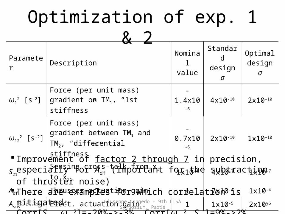
Parameter Description Nominal value
Standard design
σ
Optimal design
σ
ω12 [s-2] Force (per unit mass) gradient on TM1,
“1st stiffness” -1.4x10⁻⁶ 4x10⁻¹⁰ 2x10⁻¹⁰
ω122 [s-2] Force (per unit mass) gradient between
TM1 and TM2, “differential stiffness” -0.7x10⁻⁶ 2x10⁻¹⁰ 1x10⁻¹⁰
S21 Sensing cross-talk from x1 to x12 1x10⁻⁴ 4x10⁻⁷ 1x10⁻⁷
Adf Thruster actuation gain 1 7x10⁻⁴ 1x10⁻⁴
Asus Elect. actuation gain 1 1x10⁻⁵ 2x10⁻⁶
Optimization of exp. 1 & 2
22/05/2012
Improvement of factor 2 through 7 in precision, especially for Adf (important for the subtraction of thruster noise)
There are examples for which correlation is mitigated: Corr[S21, ω12
2]=-20%->-3%, Corr[ω122, S21]=9%->2%

Giuseppe Congedo - 9th LISA Symposium, Paris 17
Optimization of exp. 1 & 2
22/05/2012
The optimization converged to: Exp. 1: lowest (0.83 mHz) and highest (49 mHz) allowed frequencies Exp. 2: highest (49 mHz) allowed frequency (plus a slot with 0.83 mHz)

Giuseppe Congedo - 9th LISA Symposium, Paris 18
Optimization of exp. 1 & 2
22/05/2012
Optimized design:Exp. 1: 4 slots @ 0.83 mHz, 3 slots @ 49 mHzExp. 2: 1 slot @ 0.83 mHz, 6 slots @ 49 mHz
why is it so?the physical interpretation is within the system transfer matrix
11, ooi →
121, ooi →1212, ooi →
The optimization:converges to the maxima of the transfer matrixbalances the information among them
•
•
•
112, ooi →
Exp. 1
Exp. 2
•

Giuseppe Congedo - 9th LISA Symposium, Paris 19
Effect of frequency-dependences
22/05/2012
loss angle
nominal stiffness, ~-1x10⁻⁶ s-2
dielectric loss
gas damping
Simulation of the response of the system to a pessimistic range of values:
δ1, δ2 = [1x10-6,1x10-3] s-2
τ1, τ2 = [1x105,1x107] s
11, ooi →
121, ooi → 1212, ooi →However, the biggest contribution is due to gas damping, Cavalleri A. et al., Phys. Rev. Lett. 103, 140601 (2009)
112, ooi →
mHz 1 @ s 10×2< -2-112gω
( )( ) ( )[ ]2/12/12 //328/+1 13/=/= kTmππPLMβMτ
( )( ) ( )[ ]( )( ) ( )[ ] s 10×5~m/s 280cm 6.4 Pa 10×58/kg 96.1~
s 10×4~m/s 250cm 6.4 Pa 10×58/kg 96.1~91-26-
8-12-5
τ
τ
(N2, gas venting directly to space)
(Ar)
-2-10 s 10×1>2ωσ

Giuseppe Congedo - 9th LISA Symposium, Paris 20
Concluding remarks The optimization of the system calibration shows:‐ improved parameter precision‐ improved parameter correlation The optimization converges to only two relevant frequencies which
corresponds to the maxima of the system transfer matrix; this leads to a simplification of the experimental designs
Possible frequency-dependences in the stiffness constants do not impact the optimization of the system calibration
However, we must be open to possible frequency-dependences in the actuation gains [to be investigated]
The optimization of the system calibration is model-dependent, so it must be performed once we have good confidence on the model
22/05/2012

Giuseppe Congedo - 9th LISA Symposium, Paris 21
Thanks for your attention!
22/05/2012
... and to the Trento team for the laser pointer(the present for my graduation)!


![· LTPDA Toolbox 7/5/10 6:31:06 PM] LTPDA Toolbox Getting Started with …](https://img.pdfslide.us/doc/110x75/60a8833f505b3c441c582908/-ltpda-toolbox-7510-63106-pm-ltpda-toolbox-getting-started-with-.jpg)
![LTPDA Toolbox · LTPDA Toolbox 8/25/08 11:04:41 PM] Constructor examples of the AO class](https://img.pdfslide.us/doc/110x75/6132686edfd10f4dd73a6e0b/ltpda-toolbox-ltpda-toolbox-82508-110441-pm-constructor-examples-of-the-ao.jpg)


![LTPDA Toolbox · LTPDA Toolbox 7/5/10 6:31:06 PM] The Spectral Window GUI](https://img.pdfslide.us/doc/110x75/61326878dfd10f4dd73a6e0f/ltpda-toolbox-ltpda-toolbox-7510-63106-pm-the-spectral-window-gui.jpg)