Paper No.

41

THE PREDICTION OF SCALE AND COZCORROSION IN OIL FIELD SYSTEMS

J. E. OddoChampion Technologies, Inc.

P.O. Box 450499Houston, TX 77245-0499

M. B. TomsonRice University

Department of Environmental Science and Engineering -MS519P.O. BOX 1892

Houston, TX 77251-1892

ABSTRACT

This paper describes methods to predict common mineral scales and corrosion in gas and oil fields. The calculationsresult from the unification of the scale prediction methods of Oddo and Tomson and the C02 corrosion prediction methods ofde Waard and Lotz (Corrosion 93, Paper No. 69). Background development of the calculations is discussed in the paper. Thescale prediction algorithms accurately calculate many of the parameters needed for the corrosion estimations that wereproposed in the original paper by de Waard and Lotz. By including the calculated values, more accurate corrosion estimatesare obtained. The scale prediction calculations have also been updated and revised to more accurately predict mineral scaledeposition.

This paper includes field examples of scaling and corrosive production systems to illustrate the use of the methods. Theprediction model uses produced water chemistry and production volume data, as well as, flowing wellhead temperature andpressure and bottornhole temperatures and pressures to estimate temperatures and shut-in and flowing pressures in a well tocalculate the needed parameters. The model will accept a dovmhole pump and can be used with wells containing rod andelectrical submersible pumps.

The calculations are quite accurate and result in a scale/comosion model that can be used to develop field treatmentstrategies and/or assist in material selection. As is true with the de Waard and Lotz methods, the corrosion calculations predicta ‘worst case’ corrosion scenario.

INTRODUCTION

Scale and corrosion in gas and oil wells and facilities continue to be serious and costly problems. Accurate predictionalgorithms to determine the severity and location of scale deposition and corrosion allows for an early treatment programdevelopment and designing special materials into the production system to minimize the impact of the predicted problem.Production costs can then be significantly reduced.

It is essential to recognize the relationships that exist between scale and corrosion for effective corrosion prediction andtreatment. In a severely corrosive fluid environment, scales can form a protective coating over exposed surfaces, reducing orcompletely eliminating corrosion. This is the concept that resulted in the Langelier Saturation Indexl which was put forth as amethod to protect water delivery pipelines. An accurate and effective corrosion prediction algorithm must include producedwater chemistry data and accurate scale prediction algorithms as well.

The scale prediction methods used in this paper are revised equations based on the methods of Oddo and Tomson.24Oddo and Tomson derived equations from the chemical properties of the needed components of mineral scales to determinethe degree of saturation of the scale in the produced water at the temperatures, pressures and ionic strengths (a function of the

Copyright@1999byNACE International.Requestsforpermissionto publishthismanuscriptinanyform,inpartorinwholemustbe made inwritingto NACEInternational,Conferences Division,P.O. Box218340, Houston,Texas 77218-8340. The materialpresentedand the views expressed in thispaper are solelythose of the author(s) and are not necessarily endorsedby the Association.Printedin the U.S.A.

TDS) of interest. The volubility constant of a two component salt with equal charges on the cation and anion can be defined asfollows:

K,p = {CaionxAnion} (1)

where the &p is equal to the volubility constant and the {} denote activities and not concentration. The ratio of the ion activityproduct to the volubility constant is a measure of the under or oversaturation of the salt with respect to a specific solution. Asother authors have done, Langelierl for example, the degree of saturation of a scale is given by the Saturation Index or thelogl Oof the ratio of the ion activity product of the scale components to the volubility product of that particular scale. Oddo-Tomson defined a conditional volubility product that varied with temperature, pressure and ionic strength to eliminate theneed for activity coefllcients in the calculations. The Oddo-Tomson Saturation Index is defined as follows:

SI = log,~[

(CationXAnion)

KC 1 (2)

where S1 is the Saturation Index, the () denote concentration and not activity and the & is the conditional equilibriumconstant and is a function of temperature, pressure, and ionic strength.

The corrosion prediction equations used in this paper are those of de Waard and Lotz. 5 In their paper they present, as anintroduction, a mechanism for carbon dioxide corrosion and include in the paper the data horn which their equations werederived. This background information will not be repeated here. Where deviations from the original derivations are made todevelop the model presented here, it will be so noted in the text.

SCALE PREDICTION

Derivations of the scale prediction equations and the background theory have been presented elsewhere’3 and will not bepresented again in this paper. However, the fictional form of the equations used to calculate the needed volubility andstability constants has been changed from five or six terms to eight terms. Generally, the equations are of the form:

-loglO(Kc ) = a + b*T + C*T2+ d*P + e*1°”5+ PI + g*11”5+ h*T*1°”5 (3)

where Kc is the conditional constant, T is Temperature (F), P is pressure (psi) and I is the ionic strength of the produced

water (molar). The parameters for the eight terms and their associated calculated constants used in this paper are defined andshown in Table 1.

The revised recommended equations for the calculation of the Calcite Saturation Index (SIC)are shown in Table 2. Table3 shows an example of a Saturation Index calculation for gypsum. The calculation parameters are the same as defined above.The other Saturation Index calculations for the sulfate scales are done in the same manner except a different conditionalvolubility equation and the relevant metal cation are used.

CORROSION PREDICTION

De Waard and Lotz5 derived the following equation as a general prediction equation for the corrosion of carbon steel:

Vcor= ~1

1

c vma,y~+ Vreac,

(4)

where VCO, is the corrosion rate in mrnlyr., Vma.. is the mass transfer rate through the boundary layer and Vrgacfis the phase

boundary reaction rate. The equations necessary to calculate the parameters in Equation 4 areas follows:

c= Re2+2.62x10b (5)

log,o(Vrcac,)=[ 5.8-= (f )]+0.67 loglo J’(B) CO, x FPH, and273 + t

(6)

(7)

where Re is the Reynolds Number, t is temperature Celsius, fg is the figacity coefficient, P(B)C02 is the partial pressure of

COZ in bars, FP~ is the pH correction factor (see de Waard and Lotz and below), D is the diffhsion coefhcient, v is the

kinematic viscosity (m2/see), U is the liquid flow rate (mls), d is the hydraulic diameter (m), and [H2C03 ] is the total

aqueous carbon dioxide and carbonic acid concentration (M). Further, the unknowns in the above equations can be calculatedusing the following equations and by following the discussion in the text:

log10FP~ = 0.3 l(PHSa, – PH..( ) (8)

pH~a, = 5.4 – 0.66 loglO&gP(B)coz ), (for pHac, , see text)

,og10“ = 1.3272(20 - t)- 0.001053(t - 20)2

(t+ lo5)pf– 6, (t= Celsius temperature),

(9)

(lo)

V= 1X10bvpf(0.0625)pW (11)

(12)

~ ~ T(K) ~lo.,~, (T(K)= Kelvin temperature), (13)

v

([H2d= fgPco2 l(WOKM ) (14)

(NOTE: The parameters to calculate: -log10 K~ are in Table 1, and fg are in Table 2)

In the above equations T(K) is the temperature Kelvin, pH,at is the pH where FeC03 or Fe304 is at saturation in the

solution, pHac, is the actual pH of the solution, v is the dynamic viscosity (cp), pf is the density of the fluids and pW is the

density of the produced water.These and other parameters will be discussed below. The results of Equation 4 were subsequently modified in the de

Waard and Lotz paper to account for other effects on the overall corrosion rate. These effects will be briefly described in thesection below on ‘Correction Factors’ so that the reader can understand how the scale and corrosion prediction algorithmshave been combined.

Deviations in This Paper from de Waard and Lotz Derivation

The parameter ‘c’ in Equation 4 was defined by de Waard and Lotz to be a constant where c = 2.62x 10b. However, itwas found that corrosion predictions in wells with relatively low flow rates were significantly underestimated with ‘c’ equal toa constant. In this paper the ‘c’ parameter is made a fimction of the Reynolds Number (Equation 5) and is correlated with the

corrosion equations by setting ‘c’ equal to the de Waard value of 2.62x 106 at a Reynolds Number of 0.0. The ‘c’ valueincreases with the square of the Reynolds number (Equation 5). With ‘c’ defined in this manner, the corrosion equations gavereasonable results for wells with low flow rates, and the c V~a$~term (Equation 4) becomes negligible at higher flow rates as

required and noted by de Waard and Lotz.The kinematic viscosity was calculated from Equation 7. This equation differs slightly fkom the equation used by de

Waard and Lotz. The dynamic viscosity needed for the Reynolds Number calculation was obtained from the kinematicviscosity (Equation 8).6 The dynamic viscosity was corrected for the ionic strength of the water using data from Bradley, page24-17.7 A new kinematic viscosity was then calculated ffom the corrected dynamic viscosity (Equation 8) for use in thecorrosion equation. Oil viscosity was also included in the Reynolds Number calculations for the model shown in the ‘FieldExamples’ section of this paper. The oil viscosity was estimated by the method of Beggs and Robinson.8

The value of1710 in the temperature term of Equation 6 was calculated to be 1543 in the general corrosion equation byde Waard and Lotz. However, this value seemed to overestimate the corrosion rate in well systems with high Reynolds

Numbers. In the model presented here, the previously derived value of 1710 (see de Waard and Lotz) was used in thecorrosion equation. It may very well be that the value of 1543 is more correct, but more corrosion rate data is needed to testthis aspect of the model.

The parameter [H2C03 ] (Equation 7) can be calculated using equations available in the de Waard and Lotz paper.

However, all of the parameters necessary to make this calculation, the fugacity coefficient, the partial pressure of C02, and

the Henry’s Law Constant are available in the scale prediction calculations. The scale prediction calculations for thesevariables were used because they are fimctions of temperature, pressure and, ionic strength. The value obtained in the deWaard and Lotz paper is a fimction of temperature only.

In the original derivation, pHact (Equation 8) was intended to be measured or calculated using methods that are not

described in de Waard and Lotz paper. In the model developed by Oddo and Tomson2’3, the pH at any point in the system canbe calculated using the scale prediction algorithms. The calculated pH is used in this paper as pHacf. This is not a small issue

based on the practical ditllculties involved with obtaining meaningful pH values in a pressured flowing system, especially,downhole.

CORRECTION FACTORS TO THE GENERAL CORROSION EQUATION

The correction factors described below are multiplied times the results of the General Corrosion Equation (Equation 4)and decrease the amount of corrosion predicted. Neither the corrections for glycol or inhibition are included in thisdiscussion, or in the derived model.

Effects of Scale Deposition

Protective films formed by the deposition of mineral scales have long been known to reduce or eliminate corrosion inpipes. FeC03 (or Fe304 ) fihn deposition is accounted for in the de Waard and Lotz paper with the following equation:

loglo F.ca/e =2400

(f )—– 0.6 loglo #(13)co, – 6.7T(K)

(15)

where F is a general correction factor with value of 0.0< F$Cale<1.0 and &P(B)co2 is the figacity of carbon dioxide in

bars. The I%gacitycoefficient Jg, the mole ffaction ofC02 (Table 2) and the total pressure at any point (calculated flowing

pressure) are calculated when obtaining the Saturation Index for calcite scale and are used in Equation 15 to obtain a value for

‘fcale.

In addition to FeC03 (or Fe304 ) deposition, calcite scale deposits will also reduce or eliminate corrosion. Another

scale correction factor is introduced in this paper to account for the effects of calcium carbonate scale on the overall corrosionrate. The same approach taken in the above discussion was applied. A correction factor Fcalc,leis defined with values of

0.0 ~ Fcalcll.s 1.0. FCalCl,eis defined numerically as:

(.)SIC+ 0.4Fcalc,,e= 0.0 if SIC> 0.4; Fcalc,[e= 1.0 if SIC< -0.4, and -0.4< SIC ‘0.4 then Fca/cm = 1 – o g (16)

when the SZCvalue is 0.4 or greater, Fcafc,,eis set equal to 0.0 because this is the value knOWIIfrom field experience when

calcite scale will deposit in a non-turbulent production system. Local turbulence caused by a choke, a constriction in the pipe,an elbow, a drop, etc. will increase the scaling tendency locally. If calcite scale deposition is taking place, the corrosion rateshould be 0.0. Fcalcileis set equal to 1.0 when SICis equal to or less than -0.4 and is a linear fiction from 0.0 to 1“O

dependent on SIC . More information is needed regarding the transition zone between definite scaling with no corrosion, and

corrosion with no influence by the saturation of scaling materials.It is obvious that any other bulk massive scale should also inhibit corrosion, e.g. barite. However, more information

regarding the controlling S1 values for definite scale deposition of these other scales is needed. Correction terms for otherscales could be included in the model.

FOIIis introduced as a factor to correct the corrosion rate in low water cut oil wells, the water is assumed to be entrained

in the oil phase and not available to react with the tubing. De Waard and Lotz set this term equal to zero when the water cut isless than 30V0and the liquid velocity is greater than 1 mk.ec, and to 1.0 when these conditions are not met. In this paper thefactor is increased linearly to from 0.0 to 1.0 ffom water cuts of 15’?/.to 30% (Equation 17).

If the water cut is < 15’XOand the velocity of the liquids is >1 m/see., then FOi[= 0.0,

if 15°A<watercut<300A,Foil = watercut / 30 ,and

if none of these conditions are met, FO,I=1.0 (17)

FIELD APPLICATIONS OF THE MODEL

To apply the model in the field, some additional information is required. Temperatures and pressures in the well systemneed to be estimated for inclusion in the calculations at intervals in the well. In the model shown, the temperature is calculatedusing a linear assumption of temperature gradient in the wellbore. This can introduce serious errors in some systems involvingmassive carbonates, for example. However, in most cases this assumption should not affect the overall scale and corrosionpredictions dramatically.

The bottomhole shut-in pressure is calculated horn the input pressure gradient. This number is required to calculatebottomhole ‘Yo COZ in the gas phase if the ‘Yo C02 at the surface is unknown. Even if the ‘?40C02 is known at the surface, it is

wise to run the model without inputting a 0/0 C02. The water chemistry (Total Alkalinity) should be adjusted to calculate a

0/0C02 at the surface that is consistent with the measured value. This procedure will tend to reduce errors in the alkalinity

measurements, especially if the alkalinity of the weak organic acids is not measured and is unknown.Unfortunately, the contribution of the weak organic acids to the total alkalinity is not commonly measured. However for

accurate calcite scale and corrosion prediction. a value for the weak ormnic acid alkalinity is recndred or the total alkalinitymust be altered by the procedure above if the ‘AC02 is known with confidence for that particular well. A good estimate of the

weak organic acid alkalinity can be easily obtained in the field or in the laboratory while measuring total alkalinity. Thefraction of the total alkalinity due to bicarbonate can then be calculated as a function of temperature and pressure for eachpoint of interest in the system. The value required by calcite scale prediction algorithms is the true bicarbonate alkalinity. (See0ddo-Tomson3 for a complete discussion.) For these reasons, poor results will be obtained from the model by forcing a0/0 COZ measured value on a water chemistry that does not include a measurement of the contribution to the total alkalinity of

weak acids other than bicarbonate. In this case, it is better to alter the total alkalinity until a calculated 0/0 C02 is obtained

which is consistent with the measured value. If no measured 0/0 C02 value is available, it is imperative to obtain a value for

the alkalinity due to other weak acids. It is also unwise to use field average values for the YO COZin a particular well; poor

results will generally be obtained.Flowing pressures in the well were calculated using the weight of the produced gas and liquid column and the wellhead

pressure. The flowing tubing pressure is calculated from the wellhead, down the hole and, also from the bottomholeconditions up the wellbore to the wellhead pressure. When convergence is obtained to less than 1.0 psi at intervals in thewellbore, the pressure is accepted as an accurate estimate of the flowing pressure. The weights of the produced fluid columnsare corrected at intervals in the wellbore for the temperature and pressure effects on the density of water9, the solution gas andoil density’” and gas expansion. Pressure drop in the wellbore due to flow is calculated using a combination of Equations 18and 19.

yg(qg%L(P1)2 -(P2Y ‘25.2 (d,y

1

0.00001 15J,(q~~ y~LPI– P2=

(di~

(18)

(19)

where p, is the inlet pressure, p2 is the outlet pressure, ~~ is the specific gravity of the gas at standard conditions, J, is the

appropriate friction factor, L is the length of pipe in feet, T is temperature in degrees Rankine, qg is the gas flow rate in

MMCFD, d, is the pipe ID in inches, qL is the liquid flow rate in barrels per day and YLis the specific gravity of the liquid

relative to water. The friction factors for the gas phase and the liquid phase were held constant at 0.015 and 0.04, respectively,

but could be calculated.The model calculates a bubble point pressure using the solution gas calculations, if a bubble point will be encountered in

the well. The bubble point pressures calculated in the model were consistent with the bubble point pressures estimated fromthe Lmater Comelation 11calculated flow~g pres5ure5 are used for scale and corrosion calculations, since those preSSUreSme

operative during flow.

Required input into the model is shown in Table 4. The input data for the example wells shown in the remainder of thispaper are shown in Table 5. A sample input and output page is shown in Table 6. The scale and corrosion predictions are alsoshown graphically in the model as in Figure 1.

Well and Facilities

Examule 1. The first example depicted in Table 6 and Figure 1 is a well with an electrical submersible pump (ESP) setnear the level of the perforations. The model predicts that the fluids are corrosive below the level of the pump and into theESP. As is common in an ESP, the temperature of the fluids is increased fkom one end of the pump to the other. At the outputside of the pump, the system is scaling relative to calcite due to the 50 F increase in temperature in spite of the pressureincrease. As the temperature decreases in the upper parts of the well, the system becomes corrosive again and seriouscorrosion is predicted in upper parts of the well. The most serious corrosion being at about 1600 feet. Scale is again predictedin the flowlines after the choke and in the heater treater (Table 6). Note that the fluid level in this well is a negative numberindicating that the well will flow at the surface without a pump.

In the field, the pump in Examplel failed atler less than three months in the hole. When the tubing and pump were pulledfrom the hole, serious corrosion was found at the input side of the pump and in the tubing tirther up the hole, being mostsevere in the region of about 1500 feet. The pump failed due to calcite scale deposition in the pump, most severe in the midand upper sections of the pump. Scale in the surface facilities also occurred as the model predicted.

The iron concentration in the produced water was 35 mg/1 and consistent with the corrosion occurring in the well whencompared to the sandstone calculated iron concentration (Sandstone Calc. Iron, Table 6) of 3 mg/1. The sandstone calculatediron concentration is derived for sandstone reservoirs fi-om the comparative solubilities of iron and calcium carbonate, thecalcium concentration, and the overall water chemistry. The calculation does not work well in carbonate reservoirs becausethey can be deficient in iron relative to calcium due to the depositional environment.

Exanwle 2. Although the model is capable of temperature and pressure input to depict surface facilities, in the interest ofspace, only the graphical well profiles will be shown for the last three examples. The input parameters, however, are shown inTable 5. Figure 2 is a graphical depiction of the scale and corrosion profile of the second example. The well is produced witha rod pump set 4000 feet above the perforations. The well produces 50 MCFD, 25 BOPD and 200 BWPD from a depth of8,500 feet. The well fluids are corrosive throughout the entire well with the worst corrosion taking place in the area of thepump. However, the model assumes the same tubing size to the perforations. In this well there is no tubing set below thepump, and the actual corrosion rate in the 6 inch casing below the pump is much less than that shown in Figure 1. A separatecalculation can be run with 6 inch tubing size to show the corrosion rate below the pump. In addition, when entering the ID ofthe production tubing in calculations, the diameter of the rod must be subtracted fi-omthe ID.

The well depicted by Figure 2 must be treated with corrosion inhibitor evety two weeks, or failures will occur within oneto two months atler a workover. As the model shows, the most serious corrosion is in the region of the pump and is less atshallower depths.

No scale has been detected in this well which is consistent with the model predictions. The barite saturation indexincreases to 0.49 at the wellhead, but this is not sufllcient to precipitate barite scale. Laboratory experiments done at RiceUniversity suggest that the saturation index necessary to precipitate barite scale is much higher than the 0.4 S1used for calciteand in the region of 0.9.12

Figure 2A shows the same well profile as figure 2, but all of the alkalinity was attributed to bicarbonate, ignoring thealkalinity due to other weak acids. In addition, the calculated ‘XO C02 in the gas phase was ignored and the measured value of

3.4’% was input. Note the dramatic increase in scaling tendency and the decrease in the corrosion rate. The fact that thescaling tendency is so high in a liquid well downhole at the perforations should be a clue that there is a problem with the inputdata. The total alkalinity was 1586 mg/1, while the (ignored) alkalinity due to other weak acids was 1013 mg/1. Even if theweak organic acid alkalinity had not been known, a reasonable estimate for the scale/corrosion tendencies in the well could beobtained by entering values for the weak acid alkalinity until the 0/0 C02 calculated was consistent with the measured value.

Figure 2B shows the same well profile as Figs. 2 and 2A, also ignoring the alkalinity due to weak acids other thanbicarbonate. However, in this example no ‘Yo C02 was input into the model. The model calculates a VO C02 in the gas phase

of 20.5V0. The result is a predicted corrosion rate over 2.5 times as high as would be calculated with the other weak acidsincluded in the calculations. This example illustrates the importance of correcting the total alkalinity for the contributions ofother weak acids for accurate scale and corrosion predictions.

Examule 3. Figure 3 shows a rod pump well fi-omwest Texas that produces from a carbonate formation. The field hasbeen water flooded with water having a high sulfate concentration. Production of 130 MCFD, 54 BOPD and 110 BWPD isfrom 6,500 feet with the pump set at 3132 feet. The well produces two types of mineral scale. Gypsum scale is depositedshallow in the formation, in the perforations and deep in the wellbore. The well is corrosive from the pump to about 1500 feetand must be treated with corrosion inhibitor. Calcium carbonate scale is deposited in this well from the wellhead down toabout 1000 feet. In addition to the corrosion treatment, the well is squeezed periodically to inhibit scale deposition.

The model correctly predicts the scale and corrosion profiles in the well. The model predicts anhydrite scale as thethermodynamically predicted calcium sulfate phase, but it is known that gypsum ofien forms kinetically when anhydrite ispredicted thermodynamically. 13The calcium sulfate S1 threshold for scale deposition can also be shown to be lower than thatfor calcite scale in laboratory work done at Rice University. 14The numerical value appears to be about 0.2, but more workneeds to be done to determine this value accurately. However, this value appears to correctly predict the calcium sulfate scaledeposition in this well.

Examule 4. Figure 4 depicts a gas well offshore Louisiana. The well produces 4 MMCFD and 300 BWPD tlom a depthof 15,000 feet. As is common in deep gas wells, the wellbore scales with calcium carbonate at the level of the perforations andin the production tubing deep in the wellbore. The scale problem in this well was so bad that the tubing was bridgedcompletely with calcite scale near the perforations. The well was treated with coiled tubing to apply acid to the scale and acidwas flushed into the formation to bring the well back into production. The well becomes corrosive in the upper 10,000 feetwith the most severe corrosion taking place in the upper 4,500 feet of the well.

Again, the model correctly predicts the scale/corrosion profile. No barite scale has been found in this well, but baritescale was recovered downstream due to a water incompatibility problem. The iron concentration in the produced water was204 mg/1.The high iron concentration is consistent with the corrosion occurring in the well, especially when compared to thecalculated sandstone iron concentration of 7.2 mg/1.

Many gas wells scale deep in the well due to the relatively light fluid column. The temperature is hot downhole, but thepressure in the wellbore can be significantly reduced relative to the reservoir due to the light fluid column. The pressuredecrease at constant temperature is conducive to calcite scale formation.

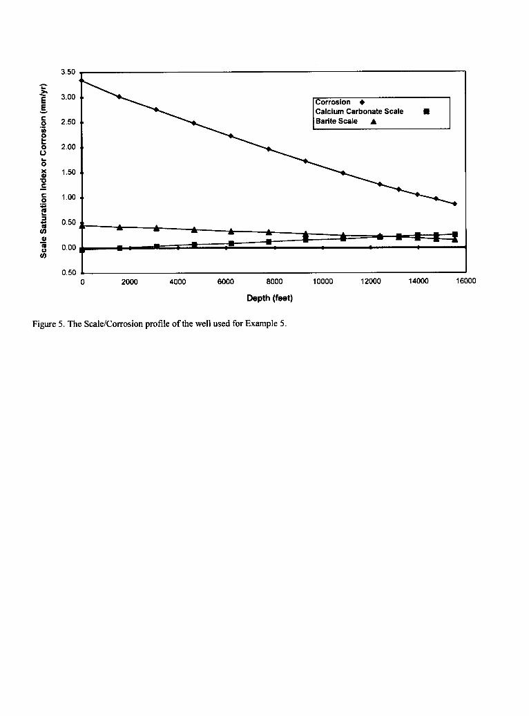
Exanmle 5. Figure 5 is the scale corrosion profile of a gas and oil well onshore Louisiana. The well produces 2.9MMCFD, 1,100 BOPD and 300 BWPD from a depth of 15,522 feet. The flowing tubing pressure is 2,000 psi at the wellhead.The scale corrosion profile is similar to Example 4 above, but the scaling tendency is less at the perforations due to theincreased pressure caused by the heavier fluid column in this example. The well has a positive scaling tendency for its entirelength which decreases the corrosion that might be expected. However, due to the high flowing tubing pressure, the well iscorrosive with the most severe corrosion taking place at the wellhead.

This well experienced abnormal pressure declines in its production history. The declines in this well were attributed toscale in the area of the perforations. This was due to the pressure decrease noted in this region atler the scale and corrosionmodel was applied. An acid job brought the well back to full production. A scale squeeze should be performed on this well toeliminate scale deposition in the future.

AVAILABILITY OF THE MODEL

The above calculations can be programmed in a spreadsheet to generate a comprehensive scale and corrosion model.Since flowing pressures are required for accurate calculations, an algorithm to calculate flowing pressures must be developedin-house, or a commercial program obtained that can be combined with the prediction equations. The resulting calculationsare accurate and useful in determining why failures have occurred, predicting tkture failures, determining chemical use rates,and in materials selection. The model is available at no charge Ilom the authors.

In addition, the ScaleSoft@model is available from Rice Universi~ that can perform S1 calculations on other scales. TheScaleSoft model will also generates a Pitzer calculation for the relative saturation of these scales and others.

ACKNOWLEDGEMENTS

The authors wish to express their thanks to Champion Technologies, Inc. for their support in the publishing of this paper.

REFERENCES

1.2.3.4.

5.

6.

7.8.9.

W. G. Langelier, J. AWWA 28 (1936) p. 1500.J. E. Oddo and M. B. Tomson, J. Pet. Tech. 34 (1982) p. 1583-1590.J. E. Oddo and M. B. Tomson, SPE Prod. and Fat. Joum. Feb. (1994) p. 47-54.S. L. He, A. T. Kan, M. B. Tomson and J. E. Oddo, “A New Interactive Sotlware for Scale Prediction, Control andManagement,” SPE Annual Tech. Conf. and Exh., Paper No. 38801, (San Antonio, TX: SPE, 1997).C. de. Waard and U. Lotz, “Prediction of COZCorrosion of Carbon Steel,” Corrosion 93, Paper No. 69, NACE, Houston,TX, 1993).J. F. Swindells, “Handbook of Chemistry and Physics,” (R. C. Weast, Cleveland, OH: The Chemical Rubber Co., 1970),p. F-36.H. B. Bradley, “Petroleum Engineering Handbook, (Richardson, TX: SPE, 1989).H. D. Beggs and J. R. Robinson, J. of Petri. Tech. Sept., (1975) p. 1140-1141.G. S. Ken, J. of Chem and Eng. Data 12 (1967): 67-68.

10. M, Vasquez and H. D. Beggs, J. Pet. Tech. June, ( 1980): p. 968-970.11. J. A. Lasater, Trans., AIME 213 (1958): pp. 379-381.12. M. B. Tomson, Personal Communication, (1997).13, J. C. Cowan and D. J. Weintritt, Water Formed Scale Deposits (Houston, TX: Gulf Publishing Co., 1976), 586 p.14. M. B. Tomson et al., “Development and Transfer of Technology Regarding Scale and NORM Scale Control,” Gas

Research Institute, Project No. 5095-250-3352, August (1996).

TABLE 1.PARAMETERS NEEDED FOR THE CALCULATION OF THE CONDITIONAL CONSTANTS.

Calcium Carbonate Scale Prediction ConstantsConditional

Constant a b c d e f g h

K~ 2.238 6.348E-3 -9.972E-6 1.234E-5 6.580E-2 -3.300E-2 4.790E-2 1.596E-4

K, 6.331 -8.278E-4 7. 142E-6 -2.564E-5 -0.491 0.379 -6.506E-2 -1.458E-3

Kz 10.511 -4.123E-3 9.297E-6 -2.118E-5 -1.255 0.867 -0.174 -1.588E-3

Kw 7.981 4.820E-3 11.183E-6 -6.973E-5 -2.725 1.183 -0.1207 -2.904E-4

K,C 4.730 -3.288E-4 5.852E-6 -1.429E-5 -0.595 0.557 -7.665E-2 -1.470E-3

K’ 3.839 5.849E-3 -8.682E-6 9.900E-7 0.170 -0.211 5.949E-2 1.716E-4

Note: K’== and is used to calculate the true bicarbonate alkalinity, see Oddo and Tomson.3K&

Sulfate Scale Prediction ConstantsConditionalConstant a b c d e f g h

K,, 2.301 1.740E-3 4.553 E-6 -7.801E-6 -3.969 2.280 -0.459 -6.037E-4

KsPg 3.599 -0.266E-3 9.029E-6 -5.586E-5 -0.847 5.240E-2 8.520E-2 -2.090E-3

KSP~ 4.053 -1.792E-3 11.400E-6 -7.070E-5 -1.734 0.562 -2. 170E-2 -6.436E-4

K spa 2.884 9.327E-3 O.188E-6 -3.400E-5 -1.994 1.267 -0.190 -3.195E-3

KSP~ 10.147 -4.946E-3 11.650E-6 -5.3 15E-5 -4.003 2.787 -0.619 - 1.850E-3

KSPCI 6.090 2.237E-3 5.739E-6 -4. 197E-5 -2.082 0.944 -8.650E-2 -1.873 E-3

where: K~ is the Henry’s Law Constant as defined in the previous papers referenced in the text, K1 is the first dissociation

constant of carbonic acid, Kz is the second dissociation constant of carbonic acid, K,w is the conditional volubility product

for calcite (calcium carbonate), K.C is the dissociation constant for acetic acid, K,, is the stability constant for the

magnesium sulfate solution complex, and K,Pg, KSph, K,w, K~Pband K~wl are the conditional volubility products for

gypsum (calcium sulfate dehydrate), hemihydrate (calcium sulfate hemihydrate), anhydrite (calcium sulfate), barite (bariumsulfate) and celestite (strontium sulfate), respectively. The equations are of the form:-loglO( Kc ) = a + b*T + C*T2+ d*P + e*1°”5+ iW + g*11’5+ h*T*1°”5.

TABLE 2.THE RECOMMENDED EQUATIONS FOR THE CALCULATION OF THE SATURATION INDICES FOR CALCITE SCALE.

Calcite Scale Saturation Index CalculationsGas Phase Present

''c='0g10Pa2%i)2l+6039+'4463x'HHCO-

pH = log10 — + 8.569+ 5.520x 10”3T – 2.830 x 10-6T2 – 1.330x 10-5P – 0.4251°”5+ 0.3461 – 1.716x 10-211’5– 1.298x 10-3T105Pygfg

where:

f~ = exp~–7.66x10-3 +8.0 xIOq TO’5–2.1 1XIO-5T~0”5 +(–5.77 x 10q +3.72 x10-5T0”5 -5.7 x10-7 T)P+(4.4x10”G -2.96 x10-7T05 +5.1 x10-9 T)P15jand

yg = Yt

[

Pf&5.O x BWPD + 10.0 x BOPD)X 10-51.0+

(T+ 460)x MMCFD 1Gas Phase Absent

I

(Ca2 ‘)( HCO~)2SIC = loglo +3.801 +8.115x1O ‘3 T+9.028x10 ‘6T2 –7.419x1O 0“5 +O.695I–1.136X1O ‘211.5 _ 1.604x 10–4T1005

C02‘5P–1.9611

c aq

[1HCO~pH = IogIo — + 6.331 –8.278 x 10-4T + 7.142 x 10-GT2 –2.564 x 10-5P – 0.4911°”5+ 0.3791 – 6.506 x 10-211”5– 1.458 x 10-3T105

c::’

where:

c:’ ‘*for wells past the bubble point and ntCoz is the total number of moles of carbon dioxide produced per day and V~~and VOare the volumes of water

and oil produced per day in liters or:

1%0 callCoz = log,oPC02– 2.212- 6.51x 10-3T + 1.019 x 10-5T2 – 1.290x 10-5P – 7.70 x 10-21°’5- 5.90x 10-2I for fluids past the gas removal point (e.g. the separator).

Measured H with gas phase present or absent

ISIC= loglo Ca2+)(HCO~)]+ pH – 2.53 + 8.943 x 10-3T + 1.886 x 10-6T2 – 4.855 x 10-5P – 1.4701°5 + 0.3161 + 5.370 x 10-2115 + 1.297 x 10-3T105

where T is temperature (F), P is pressure (psi), I is Ionic Strength (molar), Yg is the mole or volume fkaction of carbon dioxide in the gas phase at a specified temperature and

pressure, y, is the mole or volume fraction of carbon dioxide in the gas phase at room temperature and pressure and fg is the figacity of cabon dioxide gas at a specified

temperature and pressure.

TABLE 3.SAMPLE SULFATE SCALE CALCULATION.

Gwsum Scale Saturation Index Calculation

The values for the constants for the eight terms are shown in Table 1.

Calculate:

Calculate:

Calculate:

log10K,t = 2.301+ 1.740x 10-3T + 4.553 x 10-6T2 – 7.801 x lo-bp -3.9691°5 + 2.2801 – 0.4591]”5– 6.037 x 10-4T10”5

K,t = 10IOgK”

zCM =Ca2+mg/1 + Mg2+mg/1 + Sr2+mg/1 + Ba2+mg/1

40080 24304 87620 137330

SO~-mg/lCalculate: Cso, = 96000

~ ,-l+Kst(xcM-cso, )]+{(l+Kst(xcM-cso4 )}+4Kstcso4}0"5Calculate free sulfate: 0;- =

2K,t

Calculate the free metals:

[“g2+]=CM,/cMg/(l+ KS,[sO~-) ka2+l=c.a/(l+~~k~~-Dk~2+l=CSr/(I+K.~bO:-Dl~~2+l=c~a/(l+~~fCalculate the required Saturation Index, in this example, gypsum:

“g=lOg’OIF)Or

‘1. =@loka2+l’@ +3.599 –0.266x10-3 T+9.029x10AT2 –5.586x10-5P –0.847Z0’5 +5.24 x10-21 +8.52 x10-21’”5 –2.09x10-3T10’5

TABLE 4INPUT INTO THE SCALE/CORROSION PREDICTION MODEL

Wellhead Temperature (F) ID Well Casing (inches) (Req. if Annular Flow)Wellhead Pressure (psi)Separator Temperature (F)Separator Pressure (psi)Gas Production (MMCFDOil Production (BOPD)Water Production (BWPD)API Oil GravityGas Gravity Relative to AirAmbient Temperature (F)Temperature Gradient (F/100’)Top of the Perforated Interval of Interest (feet)Pressure Gradient (Shut-in psi/foot)Measured ‘YoCOZ in the Gas (Not Recommended)OD Well Tubing (inches) (Req. if Annular Flow)ID Well Tubing (inches)

Annular Flow? YiN -Pump Depth (feet) (if applicable)Pump Fluid Output Temperature (F) (if pumping)Shut-in Fluid Level (feet) (if pumping)Water Hardness (mg/1as CaC03 ) (Optional)Calcium (mg/1)Barium (mg/1)Strontium (m#l) (Optional)Iron (m#l)Weak Organic Acids (mg/1as HCO~ ) (see text)Total Alkalinity (mg/1as HCO~ )Sulfate (mg/1)Chloride (mg/1)Magnesium (mg/1) (Optional if Hardness Known)Standard Field, Well and Operator Identification

TABLE 5.INPUT VARIABLES OF THE SCALE/CORROSION MODEL FOR THE EXAMPLES SHOWN IN THE PAPER.

Example Number

Variable 1 2 3 A 5

Wellhead Temperature, F 158 75 120 2;0Wellhead Pressure, F 420 20 500MMCFD 0.262BOPD 171BWPD 237API Oil Gravity 40Gas Gravity 0.78Ambient Temperature, F 70Temp. Gradient, F per 100 feet 2.6Mid Point of Perforations, feet 5500Pressure Gradient, psi per foot 0.30Measured ‘Yo COZ, gas phase NA

ID Well Tubing, inches 2.3Pump Depth, feet 5400Pump Output Fluid Temp., F 263Shut-in Fluid Level, feet -200Hardness, mg/1 1850Calcium, mgll 270Barium, mgll 1Strontium, mg/1 38Iron, mg/1 35Magnesium, mg/1 270Weak Organic Acids, mg/1 200Total Alkalinity, mg/1 476Sulfate, mgll 260Chloride, mg/1 12360

85300.050

25200

310.73

701.6

85000.40

NA

2.14500

149-1oo143034844

NA225

3110131586

1225100

0.1354

11022

0.8070

0.806500

0.40NA

1.73132

98350

196006440

0.1NA

2.0853

7315303100

60300

-4.00.1

5942

0.6870

1.915000

0.47NA

2.6NANANANA650126NA204

360

1748

21770

20002.9

1100300

380.78

701.34

155220.47

NA

2.8NANANA

2706010204

575NA17824841

10210

102900

TABLE 6EXAMPLE INPUT/OUTPUT TO THE SCALE/CORROSION PREDICTION MODEL

Operator: Field: Well Name: Example 1

Input Variables Output Variables

Concentrations in mgll Concentrations in mg/1 I

IdVelocity (m/see) I 0.2821 I

e Pump Pressure (psi) I 10001

e Pump Pressure (psi) I 13901

Wellhead Temperature (F) 158 Hardness as tacos (Not ~.imd) 1850 Sodium 7469 Hydraulic Diameter (in) 1.15

Wellhead Pressure (psi) 420 Calcium as Calcium 270 Mg usedin Calculations 270 Liquid Veloeity (ft/see) 0.9255

Separator Temperature (F) 100 Barium Lo TDS 21141 Llqui(I

Separator Pressure (psi) 15 Strontium 38 Specific Gravity 1.015 IntakI

Ambient Temperature (F) 70 Iron 35.0 Ionic Strength (M) 0.38 Outtake4

Temp Gradient FI1OOfeet 2.60 Weak Org.

Mid Point of the Perfs. 5500 Total Alkalinity as HCOJ 476 Water Cut % 58.1

Press. Gradient (psi/ft.) 0.30 Sulfate 260.0 011Density (gmlcm’) 0.8251 Bubbl I I

Production Tubing ID (in) 2.30 Chloride.

I L 1 I I I

Production Tubing OD (in) Mess. % COZ@ 75 F and 14.7 psi’.

Moles OWDay 1228092 Calculal1 I

Casing ID (in)

..Mill---- -- ___ .. . .. . ___ ~.. -... I I

Annular Fiow? YIN Barrels Oil Produced per Day 1711

!.Acid Alkalinity as HCOJ I 2001Sandstone Calc. Iron I 3.OIIntakePump Temperature (F) I 2121

IIePoi33Lif any (psi) I NA I

~- 123601Moies Gas/Dav I 313861 lPerforation Temp. (F) I 2131

~tedBHSIP (psi) I 1650 I

lions of CnhiCFt. of (k ner Dav I~~ay 2062%OlCalculated BHFP (psi) 1020

I

..~.. I--- . . . . . .. -.-. ..J

-2001Gas Gravity

I I 1

lBaSO. Bottomhole Shut-in S1 -0.0711 1

Pump Depth (ft), if any 5400 Barrels of Water Produced per Day 237

Fluid Temp. - Pump Disch#~- 1 Ml] API oil Crnvitw 40 Calc. % C02 @ SC 1.52 HCOJ Flowing Bottomhole (m#l) 288.2

Shut-in Fluid Level (ft) 0.78 Calc. %’0 C02 @ Perfs. 1.23 Bottomhole COZFugacity Coeff. 0.861 1

‘ Input not Recommended (See Read Me) Log of Molar Calcium -2.1716

Point Calculation Calc. I Calc Static I Calc. Gas Phase Corrosion S1 S1 SI S1 Hemi- S1 S1

Description

pH

I Temn. (IO I Denth Mt) Pressure Flow Press. Present? mmlyr I CaC03 I Barite I Gypsum I Hydrate / Anhydnte I Ceiestite I Calc.

Bottomhole 213 5500 1650 io20 1.73 0.18 -0.04 -1.70 -1.67 -1.23 -0.44 5.88

PumpIntake 212 5400 1629 1000 1.78 0.18 -0.03 -1.70 -1.67 -1.23 -0.44 5.88

PumpOutput 263 5400 1629 1390 0.00 0.74 -0.12 -1.63 -1.57 -0.92 -031 5.92

247 4590 1454 1215 0.00 0.58 -0.10 -1.65 -1.60 -1.01 -0.35 5,92

242 4320 1396 1157 0.00 0.53 -0.09 -1.66 -1.61 -1.04 -0.36 5.93

232 3780 1288 1049 0.00 0.42 -0.07 -1.67 -1.63 -1.11 -0.39 5.93

221 3240 1184 945 0.58 0.32 -0.05 -1.69 -1.65 -1.17 -0.41 5.93

211 2700 1083 844 1.41 0.22 -0.0 I I 1 1 1

x-u-l ?160 QWi 747 2.34 0.12 0.00 -1.71 -1.68 -130 -0.47 5.95 1

)2 I -1.70 I -1.66 I -1.24 I -0.44 I 5.94 I

-.,. ---- ---190 1620 893 654 2.69 0.03 0.03 -1.72 -1.69 -1.37 -0.49 5.96

179 1080 804 565 2.59 -0.06 0.06 -1.73 -1.70 -1.44 -0.51 5.98

169 540 719 480 2.32 -0.14 0.09 -1.73 -1.70 -1.51 -0.54 6.00

Wellhead 158 0 659 420 2.10 -0.23 0.12 -1.74 -1.71 -1.58 -0.56 6.02

Flowline 158 0 NIA 400 1.96 -0.21 0.12 -1.74 -1.71 -1.58 -0.S6 6.04

Choke 158 0 NIA 50 0.00 0.65 0.14 -1.72 -1.69 -1.57 -0.55 6.89

InTreater 140 0 NIA 15 0.00 0.92 0.20 -1.73 -1.70 -1.69 -0.59 7.34

Treater 180 0 NIA 15 0.00 1.48 0.08 -1.69 -1.66 -1.41 -0.49 7.49

100 0 N/A 15 N 0.00 0.35 0.34 -1.74 -1.71 -1.97 -0.68 7.18

3.00

2.50

2.00

1.50

1.00

0.50

0.00

-0.50

-1.00

-1.50

-2.00 to 1000 2000 3000 4000 5000 6000

Depth (feet)

FIGURE 1- Example of the graphical output of the Scale/Corrosion Prediction Model, and the well used as Example 1.Note the temperature increase in the pump causes an increase in calcite scaling tendency and a decrease in corrosion rateand in barite scaling tendency.

5.00

4,00

3.00

2.00

1.00

A .

0.00 ‘

t .00 Jo 1000 2000 3000 4000 5000 6000 7000 8000 9000

Depth (feet)

FIGURE 2- The Scale/Corrosion profile of the well used for Example 2. The model calculates a percent carbon dioxide inthe gas phase of 3.38°76vs. a measured value of 3.4%.

1.00 ,

0.901

0.80 ,8

0.70 ,,

0,60 ut

0.50 8

0,40 ,D

0.30 ,,

0.20 aD

0.10 t,

0.004 I

0.10 Jo 1000 2000 3000 4000 5000 6000 7000 8000 9000

Depth (feet)

FIGURE 2A. - The Scale/Corrosion profile of the well used for Example 2 ignoring the alkalinity due to weak acids andattributing all of the alkalinity to bicarbonate. Although, the model calculates a percent carbon dioxide in the gas phase of20.5%. the actual measured value of carbon dioxide of 3.4’%was inuut into the model. This results in a much decreasedcorrosion rate and a substantial increase in the calcite scaling tendency. Note the high scaling tendency at downholeconditions in an oil and water well which is a strong indication that there is a problem with the input data.

12.00 k

10.00 a,

8.00. v

6.00 I.

4.00 ..

2.00. ,

0.00 t

2.00 Jo 1000 2000 3000 4000 5000 6000 7000 8000 9000

Depth (feet)

FIGURE 2B - The Scale/Corrosion profile of the well used for Example 2 ignoring the alkalinity do to weak acids andattributing all of the alkalinity to bicarbonate. The model calculates a percent carbon dioxide in the gas phase of 20.50/.resulting in the very high corrosion rates illustrated.

~ c)S

cale

Satu

rati

onIn

dex

or

Co

rro

sio

n(m

m/y

r)

5MA

oA

.@.

mm

Ao

00

00

00

00

00

00

00

00

0

Scal

eSa

tura

tion

Ind

exo

rC

orr

osi

on

(mm

lyr)

o0

0m o

0U

Io

00

ino

0

3.50 ~ 1

3.00

2.50

2.00

1,50

1.00

0.50

0.00

0.50 J Jo 2000 4000 6000 8000 10000 12000 14000 16000

Depth (feet)

Figure 5. The Scale/Corrosion profile of the well used for Example 5.