Embed Size (px)
Citation preview
37
2.1 Introduction
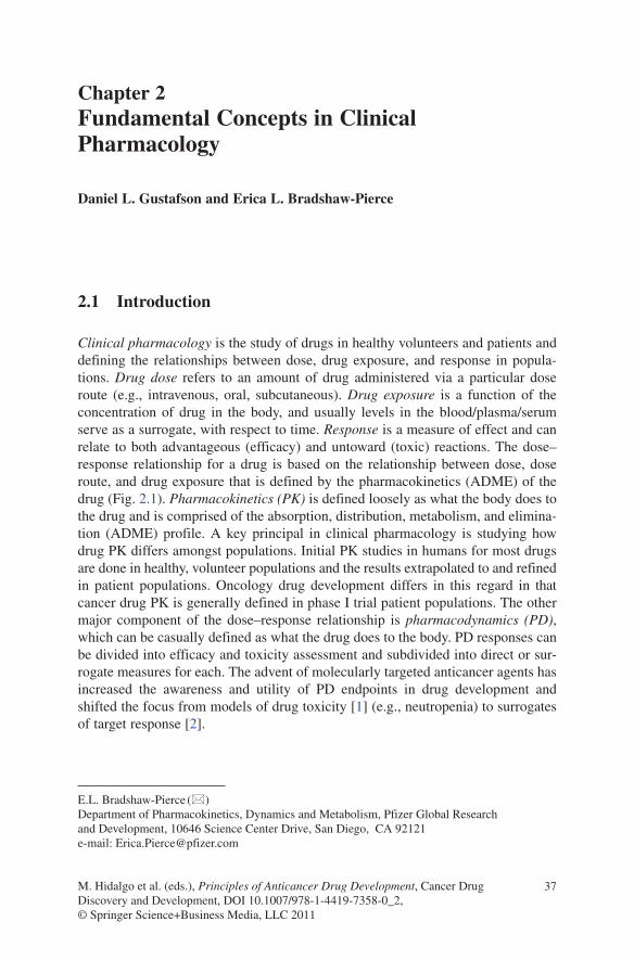
Clinical pharmacology is the study of drugs in healthy volunteers and patients and defining the relationships between dose, drug exposure, and response in popula-tions. Drug dose refers to an amount of drug administered via a particular dose route (e.g., intravenous, oral, subcutaneous). Drug exposure is a function of the concentration of drug in the body, and usually levels in the blood/plasma/serum serve as a surrogate, with respect to time. Response is a measure of effect and can relate to both advantageous (efficacy) and untoward (toxic) reactions. The dose–response relationship for a drug is based on the relationship between dose, dose route, and drug exposure that is defined by the pharmacokinetics (ADME) of the drug (Fig. 2.1). Pharmacokinetics (PK) is defined loosely as what the body does to the drug and is comprised of the absorption, distribution, metabolism, and elimina-tion (ADME) profile. A key principal in clinical pharmacology is studying how drug PK differs amongst populations. Initial PK studies in humans for most drugs are done in healthy, volunteer populations and the results extrapolated to and refined in patient populations. Oncology drug development differs in this regard in that cancer drug PK is generally defined in phase I trial patient populations. The other major component of the dose–response relationship is pharmacodynamics (PD), which can be casually defined as what the drug does to the body. PD responses can be divided into efficacy and toxicity assessment and subdivided into direct or sur-rogate measures for each. The advent of molecularly targeted anticancer agents has increased the awareness and utility of PD endpoints in drug development and shifted the focus from models of drug toxicity [1] (e.g., neutropenia) to surrogates of target response [2].
E.L. Bradshaw-Pierce (*) Department of Pharmacokinetics, Dynamics and Metabolism, Pfizer Global Research and Development, 10646 Science Center Drive, San Diego, CA 92121 e-mail: [email protected]
Chapter 2Fundamental Concepts in Clinical Pharmacology
Daniel L. Gustafson and Erica L. Bradshaw-Pierce
M. Hidalgo et al. (eds.), Principles of Anticancer Drug Development, Cancer Drug Discovery and Development, DOI 10.1007/978-1-4419-7358-0_2, © Springer Science+Business Media, LLC 2011
38 D.L. Gustafson and E.L. Bradshaw-Pierce
2.2 Glossary
Terms that are commonly used in PK and PD modeling and data analysis are listed and defined below along with the common abbreviation used to represent them.
2.2.1 Pharmacokinetic Terms
Area under the curve (AUC) – A measure of drug exposure that is calculated as the product of plasma drug concentration and time. Calculation of the AUC can be done by geometric calculation or by integration of fitted equations.
Bioavailability (F) – The fraction of an administered dose that reaches the systemic circulation. Calculated as a ratio of AUC following dosing via a given dose route to the AUC of the same dose given intravenously.
Clearance (CL) – A factor that relates drug elimination to the plasma drug concentration. Calculated using the dose administered divided by the subsequent measured AUC.
Elimination rate constant (kel) – The slope of the terminal phase of the plasma
drug concentration vs. time curve.Elimination half-life (t
1/2) – The time it takes plasma drug concentration to
decrease by half during the terminal elimination phase.Maximum concentration (C
max) – The maximum concentration of drug obtained
in the plasma.Time to maximum concentration (T
max) – The time it takes post dosing to reach
a maximum plasma concentration.Volume of distribution – A factor that relates the amount of drug in the body
to the concentration of drug in the plasma. This term can be calculated as an initial volume (V
D), during the terminal phase (V), or under steady-state
conditions (Vss).
Pharmacokinetics
Dose
AbsorptionDistribution ResponseMetabolismElimination
Fig. 2.1 Relationship of pharmacokinetics to dose–response
392 Fundamental Concepts in Clinical Pharmacology
2.2.2 Pharmacodynamic Terms
Affinity – The strength of the interaction between a receptor and a ligand. This interaction is described mathematically in terms of an association or dissociation constant.
Efficacy – The capacity of a drug to induce a therapeutic effect.Intrinsic activity – The ability of a drug to induce a response at the level of a
specific molecular target.Maximum response (E
max) – The largest response that a given drug can elicit at
optimal concentrations.Potency – The concentration of a given drug that elicits a specific level of
response. This term is used as a means of comparing the ability of compounds to induce a given response.
Response (E) – A measured physiologic effect induced by a given concentration or dose of a drug. Often the measured response is a function of penetration of drug to the site of action as well as the molecular interactions and cascades that proceed.
2.2.3 Modeling Terms
Compartmental modeling – Dividing the body into nonspecific body region group-ings (compartments) that share similar rates of drug movement in and out for the purpose of describing plasma concentration vs. time data.
Linear pharmacokinetics – Dose proportionality in plasma drug levels and expo-sure (AUC) such that clearance and volume of distribution do not change with dose.
Noncompartmental modeling – The use of geometric and algebraic relationships to calculate pharmacokinetic parameters from plasma concentration vs. time data. Although the basis of noncompartmental modeling is classical statistical moment theory, current use of this approach in pharmacokinetics is generally limited to calculation of pharmacokinetic parameters using model-independent approaches and a series of equations for calculating common pharmacokinetic parameters.
Nonlinear pharmacokinetics – The use of saturable (capacity-limited) equations to describe plasma concentration vs. time data in cases where drug absorption and/or elimination does not follow a first-order rate. In these cases, plasma drug concentration and drug exposure are not dose proportional.
Population pharmacokinetic modeling – The incorporation of population characteristics into pharmacokinetic models in order to understand the sources of variability associated with drug exposure within a population.
Physiologically based pharmacokinetics (PBPK) – A mathematical model-ing technique incorporating physiological and physio-chemical properties to describe the absorption, distribution, metabolism, and elimination of drugs.
40 D.L. Gustafson and E.L. Bradshaw-Pierce
Unlike compartmental modeling, PBPK models are comprised of compartments that represent organ systems and attribute appropriate physiological and metabolic properties to that compartment.
2.3 Sampling Schedule and Study Design
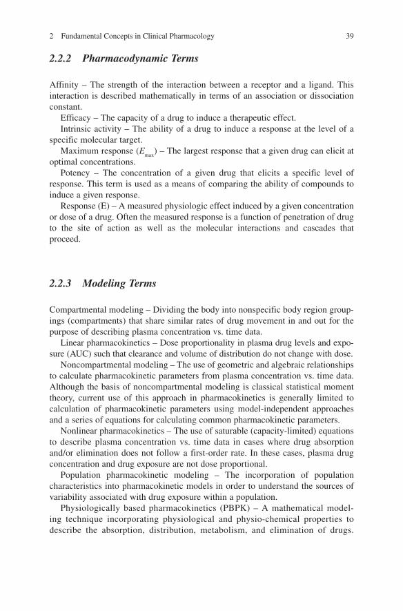
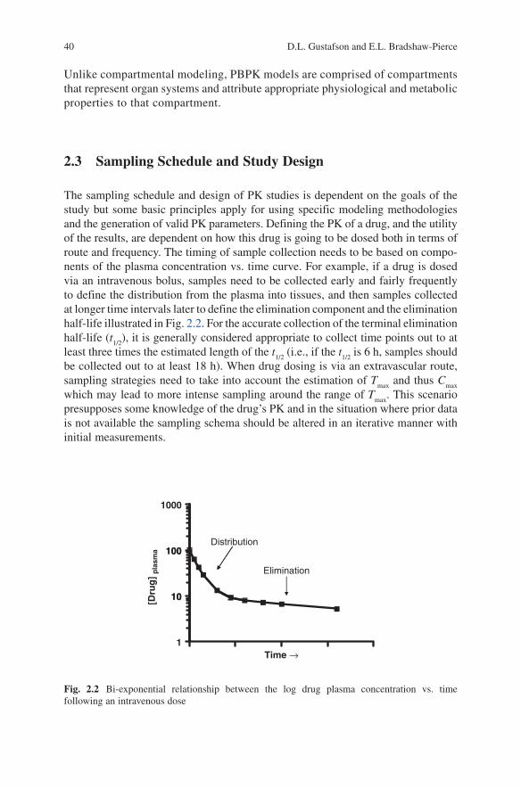
The sampling schedule and design of PK studies is dependent on the goals of the study but some basic principles apply for using specific modeling methodologies and the generation of valid PK parameters. Defining the PK of a drug, and the utility of the results, are dependent on how this drug is going to be dosed both in terms of route and frequency. The timing of sample collection needs to be based on compo-nents of the plasma concentration vs. time curve. For example, if a drug is dosed via an intravenous bolus, samples need to be collected early and fairly frequently to define the distribution from the plasma into tissues, and then samples collected at longer time intervals later to define the elimination component and the elimination half-life illustrated in Fig. 2.2. For the accurate collection of the terminal elimination half-life (t
1/2), it is generally considered appropriate to collect time points out to at
least three times the estimated length of the t1/2
(i.e., if the t1/2
is 6 h, samples should be collected out to at least 18 h). When drug dosing is via an extravascular route, sampling strategies need to take into account the estimation of T
max and thus C
max
which may lead to more intense sampling around the range of Tmax
. This scenario presupposes some knowledge of the drug’s PK and in the situation where prior data is not available the sampling schema should be altered in an iterative manner with initial measurements.
Distribution100
1000
Elimination
10
100
[Dru
g]
pla
sma
1
10
Time →
Fig. 2.2 Bi-exponential relationship between the log drug plasma concentration vs. time following an intravenous dose
412 Fundamental Concepts in Clinical Pharmacology
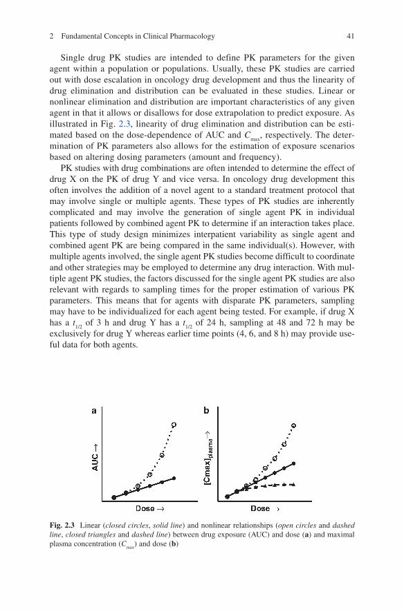
Single drug PK studies are intended to define PK parameters for the given agent within a population or populations. Usually, these PK studies are carried out with dose escalation in oncology drug development and thus the linearity of drug elimination and distribution can be evaluated in these studies. Linear or nonlinear elimination and distribution are important characteristics of any given agent in that it allows or disallows for dose extrapolation to predict exposure. As illustrated in Fig. 2.3, linearity of drug elimination and distribution can be esti-mated based on the dose-dependence of AUC and C
max, respectively. The deter-
mination of PK parameters also allows for the estimation of exposure scenarios based on altering dosing parameters (amount and frequency).
PK studies with drug combinations are often intended to determine the effect of drug X on the PK of drug Y and vice versa. In oncology drug development this often involves the addition of a novel agent to a standard treatment protocol that may involve single or multiple agents. These types of PK studies are inherently complicated and may involve the generation of single agent PK in individual patients followed by combined agent PK to determine if an interaction takes place. This type of study design minimizes interpatient variability as single agent and combined agent PK are being compared in the same individual(s). However, with multiple agents involved, the single agent PK studies become difficult to coordinate and other strategies may be employed to determine any drug interaction. With mul-tiple agent PK studies, the factors discussed for the single agent PK studies are also relevant with regards to sampling times for the proper estimation of various PK parameters. This means that for agents with disparate PK parameters, sampling may have to be individualized for each agent being tested. For example, if drug X has a t
1/2 of 3 h and drug Y has a t
1/2 of 24 h, sampling at 48 and 72 h may be
exclusively for drug Y whereas earlier time points (4, 6, and 8 h) may provide use-ful data for both agents.
Fig. 2.3 Linear (closed circles, solid line) and nonlinear relationships (open circles and dashed line, closed triangles and dashed line) between drug exposure (AUC) and dose (a) and maximal plasma concentration (C
max) and dose (b)
42 D.L. Gustafson and E.L. Bradshaw-Pierce
PK studies are often also carried out in special populations with the intent of deter-mining if specific population characteristics influence drug elimination or distribu-tion. Examples of population characteristics often studied include organ function and metabolic polymorphisms. These types of studies are dependent on the availability of individuals within the population of interest and what changes in PK are anticipated. For example, if a population is deficient in a specific metabolic pathway and hepatic drug elimination is expected to be decreased, this can influence the t
1/2 as well as the
Tmax
and can change the sampling schedule that should be utilized. These consider-ations will be drug and population characteristic dependent and re-emphasize the importance of taking into account PK characteristics in study and sampling design.
Another consideration when determining the sampling schedule is the analytical sensitivity of the assay that will be used to measure drug levels in samples. Utilization of more sensitive methods may allow for drug measurements at later time points and this can influence the calculated PK parameters [3] and the ability to sample out to three times the length of the elimination phase. Assay sensitivity, t
1/2 and the
dose being given influence what time points can be measured and should be con-sidered when a sampling schema is being designed.
2.4 Patient Numbers and Sampling Intensity
The number of patients required for a given study in clinical pharmacology is dependent on the question being addressed. For a typical phase I dose-escalation study, the purpose of the PK component is to determine drug exposure in the con-text of the toxicity being assessed at a given dose level. The number of samples per dose level obtained in phase I studies is dependent on the dose-escalation schedule being used and generally ranges from 1 to 6 patients. These dose-escalation studies can provide valuable information regarding the PK of a given agent, as shown in Fig. 2.3 for linear vs. nonlinear, regardless of the small number of patients within each dose level. Clinical pharmacology studies addressing differences between populations or to determine the presence or absence of a drug interaction would require sample numbers sufficient to either support or reject the null hypothesis based on data variability, degree of change in a parameter, and the level of statistical significance required. Power calculations can be performed to help determine the necessary sample size for these types of comparisons. However, most phase I study sample sizes are based on determining the maximum tolerated dose and not based on pharmacokinetic comparisons.
Sampling intensity is a function of both the needs of the study and the reality of clinical sampling. In the outpatient setting, collecting 12 and/or 16 h samples is technically limiting and sampling between 8 and 24 h postdosing is not feasible except under special circumstances. Sampling intensity can also be influenced by the data analysis methods intended to be used. For example, if the data is to be analyzed by a three-compartment model (discussed below), the number of unknown variables
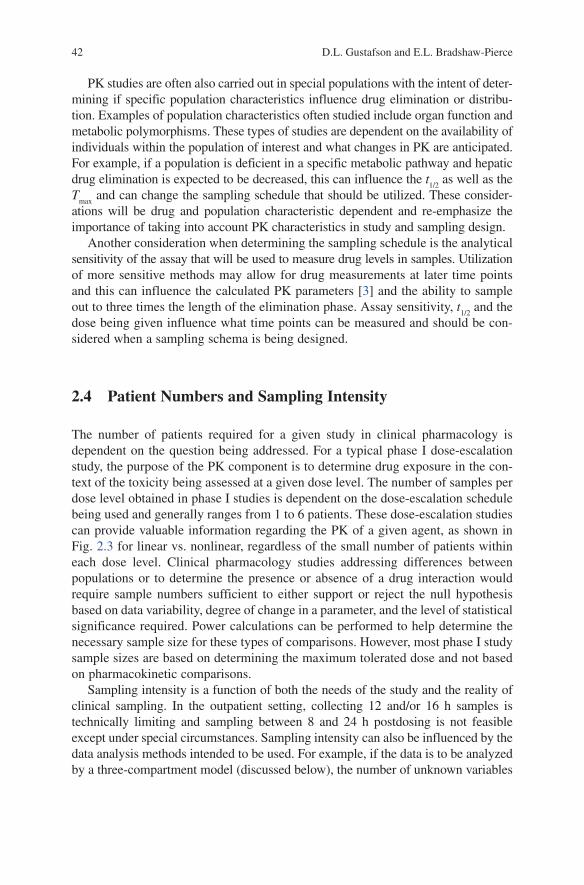
432 Fundamental Concepts in Clinical Pharmacology
to be solved is 6 and thus the minimum number of samples required is 7 and they need to be distributed within the three specific phases of drug distribution, equilibra-tion, and elimination for the accurate estimation of model parameters (Fig. 2.4). The intensity of sampling is also dependent on the time-frame within which each of these phases occurs which is compound dependent. Generally, the distribution phase is rapid, meaning frequent, more intense sampling during this early phase and more protracted sampling for the slower subsequent phases. Shown in Fig. 2.4 is sampling within the context of (a) two- and (b) three-compartment modeling to allow for proper curve resolution and accurate parameter estimation. As stated earlier, optimal estimation of the elimination phase includes sampling out to three times the elimina-tion half-life. Sampling intensity is also a function of the amount of sample collected as the amount of blood collected is limited by patient size and other characteristics.
2.5 What is the Goal of the PK Study?
It is critically important to determine the goals of PK studies a priori? The goals of the study will dictate the design of the study, including the frequency and intensity of sampling. If the purpose is to define the PK parameters and drug exposure of a drug in humans, then proper sampling strategies, as discussed earlier, should be put in place to assure that parameters can be accurately estimated. If the goal is to determine if limited sampling strategies can be utilized to determine a PK param-eter that correlates with drug response or toxicity and employ this strategy in thera-peutic drug monitoring, then the study must be designed in the context of determining what PK parameter correlates to a specific drug response and how best to estimate that PK parameter with regards to patient sampling. If a study is
1000
a b
Distribution Phase3-4 sampling times
Distribution Phase3-4 sampling times
Equilibration Phase3-4 sampling times
100
[Dru
g] p
lasm
a
[Dru
g] p
lasm
a
Elimination Phase3-4 sampling times
0 6 12 18 241
10
1000
100
1
10Elimination Phase3-4 sampling times
0 6 12 18 24Time
0 6 12 18 24 30 36 42 48Time
Fig. 2.4 Phases and recommended sampling density within each phase for a bi-exponential two-compartment model (a) and a tri-exponential three-compartment (b)
44 D.L. Gustafson and E.L. Bradshaw-Pierce
intended to determine if a drug interaction is taking place (i.e., drug X alone vs. drug X with drug Y), then it must be determined if the PK will be done with drug X alone and with drug X and Y or whether just the combination of drug X and Y will be measured and the values compared to historic or literature values. An important component in planning these types of studies is the quality and type of historical data that will be used if that avenue of study design is chosen. In order to compare newly generated PK data with data from a previous study, it is important to note that similar dose ranges should be compared unless it is clear that the PK of the agent being studied is linear with dose, that the same modeling methodology should be used for data analysis, and that the sampling schedule should be similar to that employed in the earlier study.
2.6 Pharmacokinetics
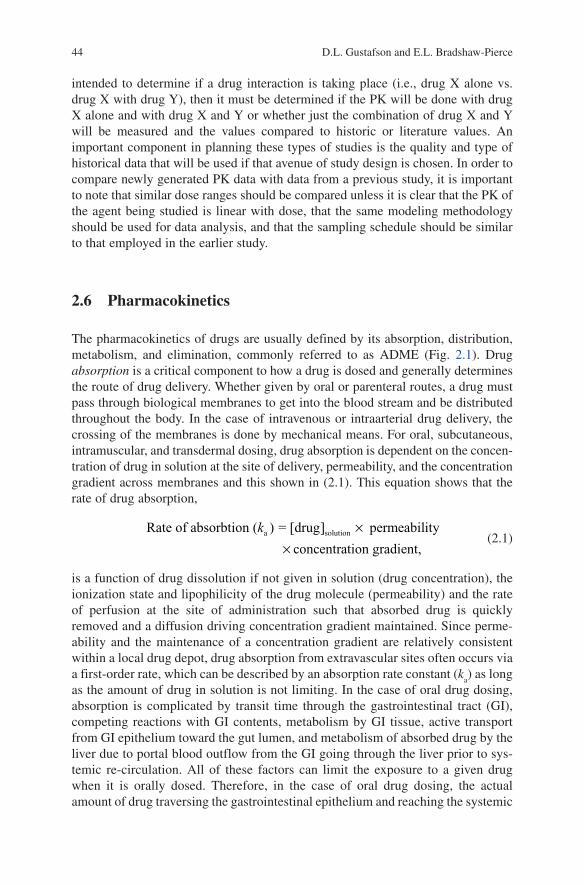
The pharmacokinetics of drugs are usually defined by its absorption, distribution, metabolism, and elimination, commonly referred to as ADME (Fig. 2.1). Drug absorption is a critical component to how a drug is dosed and generally determines the route of drug delivery. Whether given by oral or parenteral routes, a drug must pass through biological membranes to get into the blood stream and be distributed throughout the body. In the case of intravenous or intraarterial drug delivery, the crossing of the membranes is done by mechanical means. For oral, subcutaneous, intramuscular, and transdermal dosing, drug absorption is dependent on the concen-tration of drug in solution at the site of delivery, permeability, and the concentration gradient across membranes and this shown in (2.1). This equation shows that the rate of drug absorption,
a solutionRate of absorbtion ( ) = [drug] permeability
concentration gradient,
××
k (2.1)
is a function of drug dissolution if not given in solution (drug concentration), the ionization state and lipophilicity of the drug molecule (permeability) and the rate of perfusion at the site of administration such that absorbed drug is quickly removed and a diffusion driving concentration gradient maintained. Since perme-ability and the maintenance of a concentration gradient are relatively consistent within a local drug depot, drug absorption from extravascular sites often occurs via a first-order rate, which can be described by an absorption rate constant (k
a) as long
as the amount of drug in solution is not limiting. In the case of oral drug dosing, absorption is complicated by transit time through the gastrointestinal tract (GI), competing reactions with GI contents, metabolism by GI tissue, active transport from GI epithelium toward the gut lumen, and metabolism of absorbed drug by the liver due to portal blood outflow from the GI going through the liver prior to sys-temic re-circulation. All of these factors can limit the exposure to a given drug when it is orally dosed. Therefore, in the case of oral drug dosing, the actual amount of drug traversing the gastrointestinal epithelium and reaching the systemic
452 Fundamental Concepts in Clinical Pharmacology
circulation is tempered by these competing processes whereas drug absorption from parenteral sites is often simply a function of permeability across cellular membranes and access to the circulation. The measure of drug absorption and exposure from extravascular sites is termed bioavailability (F) and is determined by (2.2) and represents simply the drug exposure (AUC) following the extravascu-lar dose in comparison to drug exposure following intravenous (IV) dosing.
extravascular IV
IV extravascular
AUC Dose.
AUC Dose
×=
×F
(2.2)
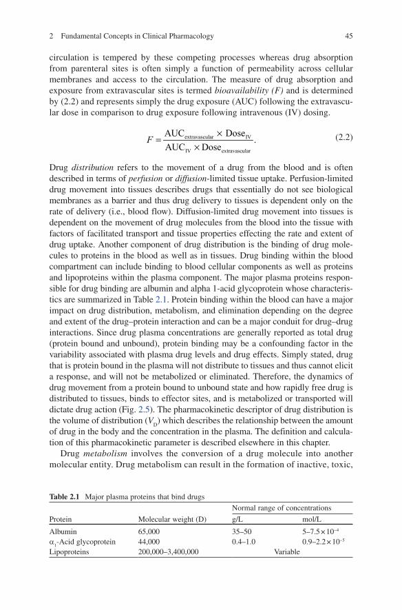
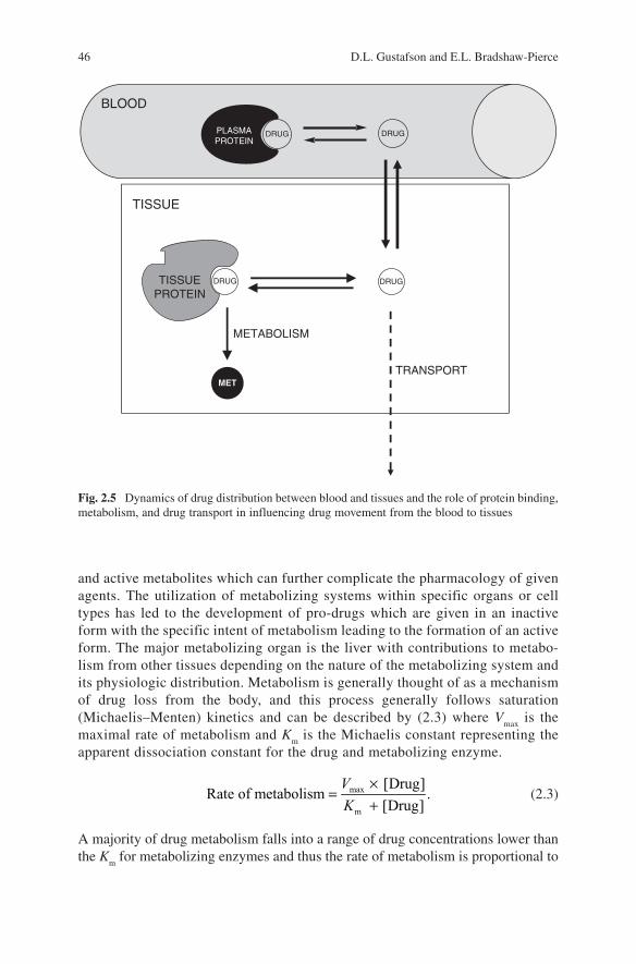
Drug distribution refers to the movement of a drug from the blood and is often described in terms of perfusion or diffusion-limited tissue uptake. Perfusion-limited drug movement into tissues describes drugs that essentially do not see biological membranes as a barrier and thus drug delivery to tissues is dependent only on the rate of delivery (i.e., blood flow). Diffusion-limited drug movement into tissues is dependent on the movement of drug molecules from the blood into the tissue with factors of facilitated transport and tissue properties effecting the rate and extent of drug uptake. Another component of drug distribution is the binding of drug mole-cules to proteins in the blood as well as in tissues. Drug binding within the blood compartment can include binding to blood cellular components as well as proteins and lipoproteins within the plasma component. The major plasma proteins respon-sible for drug binding are albumin and alpha 1-acid glycoprotein whose characteris-tics are summarized in Table 2.1. Protein binding within the blood can have a major impact on drug distribution, metabolism, and elimination depending on the degree and extent of the drug–protein interaction and can be a major conduit for drug–drug interactions. Since drug plasma concentrations are generally reported as total drug (protein bound and unbound), protein binding may be a confounding factor in the variability associated with plasma drug levels and drug effects. Simply stated, drug that is protein bound in the plasma will not distribute to tissues and thus cannot elicit a response, and will not be metabolized or eliminated. Therefore, the dynamics of drug movement from a protein bound to unbound state and how rapidly free drug is distributed to tissues, binds to effector sites, and is metabolized or transported will dictate drug action (Fig. 2.5). The pharmacokinetic descriptor of drug distribution is the volume of distribution (V
D) which describes the relationship between the amount
of drug in the body and the concentration in the plasma. The definition and calcula-tion of this pharmacokinetic parameter is described elsewhere in this chapter.
Drug metabolism involves the conversion of a drug molecule into another molecular entity. Drug metabolism can result in the formation of inactive, toxic,
Table 2.1 Major plasma proteins that bind drugs
Normal range of concentrations
Protein Molecular weight (D) g/L mol/L
Albumin 65,000 35–50 5–7.5 × 10⁻⁴
a1-Acid glycoprotein 44,000 0.4–1.0 0.9–2.2 × 10⁻⁵
Lipoproteins 200,000–3,400,000 Variable
46 D.L. Gustafson and E.L. Bradshaw-Pierce
and active metabolites which can further complicate the pharmacology of given agents. The utilization of metabolizing systems within specific organs or cell types has led to the development of pro-drugs which are given in an inactive form with the specific intent of metabolism leading to the formation of an active form. The major metabolizing organ is the liver with contributions to metabo-lism from other tissues depending on the nature of the metabolizing system and its physiologic distribution. Metabolism is generally thought of as a mechanism of drug loss from the body, and this process generally follows saturation (Michaelis–Menten) kinetics and can be described by (2.3) where V
max is the
maximal rate of metabolism and Km is the Michaelis constant representing the
apparent dissociation constant for the drug and metabolizing enzyme.
max
m
[Drug]Rate of metabolism .
[Drug]
×=
+V
K (2.3)
A majority of drug metabolism falls into a range of drug concentrations lower than the K
m for metabolizing enzymes and thus the rate of metabolism is proportional to
BLOOD
PLASMAPROTEIN
DRUG DRUG
TISSUE
DRUGTISSUEPROTEIN
DRUG
METABOLISM
TRANSPORTMET
Fig. 2.5 Dynamics of drug distribution between blood and tissues and the role of protein binding, metabolism, and drug transport in influencing drug movement from the blood to tissues
472 Fundamental Concepts in Clinical Pharmacology
drug concentration and follows a first-order rate as described by (2.4). The term V
max/K
m represents a constant
max
m
Rate of metabolism [Drug],= ×V
K (2.4)
term with a rate (concentration/time) divided by concentration, resulting in units of time−1, which are the units of a first-order rate constant. In rare cases where the concentration of a drug is closer to or greatly exceeds the K
m of a metabolizing
system, the rate of drug metabolism will not be dose proportional and will result in either zero-order (2.5) or
maxRate of metabolism ,= V (2.5)
saturation characteristics (2.3). In cases where drug-metabolizing systems are satu-rated and metabolism fails to be dose proportional, the relationships between dose and drug exposure become nonlinear and difficult to predict.
Many drugs are metabolized by multiple metabolic pathways. Assuming that there is no interaction between the metabolic pathways, the total drug metabolism is simply the sum of the individual pathways. Drug metabolism is a major point of drug interaction due to a number of factors including competition for the active site of a metabolizing enzyme leading to competitive inhibition based on the affinity of each substrate. Other points of drug interaction can include the induction of drug-metabolizing enzymes which can lead to a proportional increase in the rate of drug metabolism. As stated earlier, drug metabolism is not necessarily synonymous with drug inactivation due to many drug metabolites being active and potentially toxic. Therefore, the role of metabolism in inactivation or activation of a given drug in terms of both efficacy and toxicity must be considered.
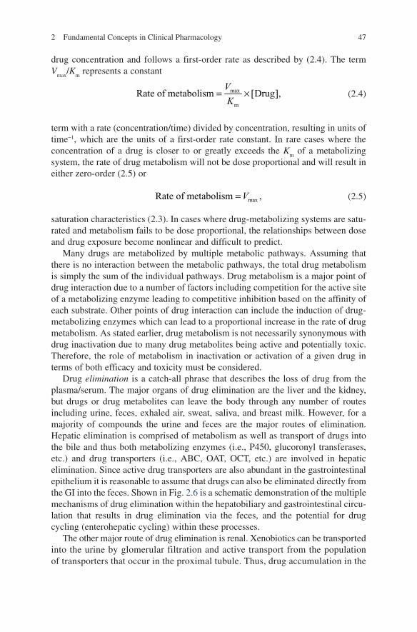
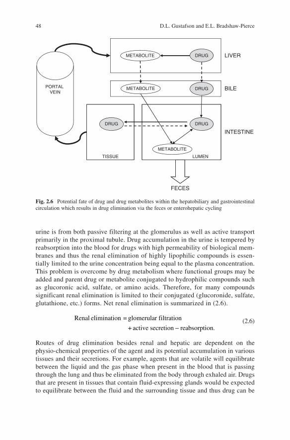
Drug elimination is a catch-all phrase that describes the loss of drug from the plasma/serum. The major organs of drug elimination are the liver and the kidney, but drugs or drug metabolites can leave the body through any number of routes including urine, feces, exhaled air, sweat, saliva, and breast milk. However, for a majority of compounds the urine and feces are the major routes of elimination. Hepatic elimination is comprised of metabolism as well as transport of drugs into the bile and thus both metabolizing enzymes (i.e., P450, glucoronyl transferases, etc.) and drug transporters (i.e., ABC, OAT, OCT, etc.) are involved in hepatic elimination. Since active drug transporters are also abundant in the gastrointestinal epithelium it is reasonable to assume that drugs can also be eliminated directly from the GI into the feces. Shown in Fig. 2.6 is a schematic demonstration of the multiple mechanisms of drug elimination within the hepatobiliary and gastrointestinal circu-lation that results in drug elimination via the feces, and the potential for drug cycling (enterohepatic cycling) within these processes.
The other major route of drug elimination is renal. Xenobiotics can be transported into the urine by glomerular filtration and active transport from the population of transporters that occur in the proximal tubule. Thus, drug accumulation in the
48 D.L. Gustafson and E.L. Bradshaw-Pierce
urine is from both passive filtering at the glomerulus as well as active transport primarily in the proximal tubule. Drug accumulation in the urine is tempered by reabsorption into the blood for drugs with high permeability of biological mem-branes and thus the renal elimination of highly lipophilic compounds is essen-tially limited to the urine concentration being equal to the plasma concentration. This problem is overcome by drug metabolism where functional groups may be added and parent drug or metabolite conjugated to hydrophilic compounds such as glucoronic acid, sulfate, or amino acids. Therefore, for many compounds significant renal elimination is limited to their conjugated (glucoronide, sulfate, glutathione, etc.) forms. Net renal elimination is summarized in (2.6).
−
Renal elimination = glomerular filtration
+ a ct ive secretion reabsorption. (2.6)
Routes of drug elimination besides renal and hepatic are dependent on the physio-chemical properties of the agent and its potential accumulation in various tissues and their secretions. For example, agents that are volatile will equilibrate between the liquid and the gas phase when present in the blood that is passing through the lung and thus be eliminated from the body through exhaled air. Drugs that are present in tissues that contain fluid-expressing glands would be expected to equilibrate between the fluid and the surrounding tissue and thus drug can be
DRUG LIVER
DRUG
METABOLITE
BILE
DRUG
METABOLITE
DRUG
INTESTINE
LUMENTISSUE
FECES
PORTAL VEIN
METABOLITE
Fig. 2.6 Potential fate of drug and drug metabolites within the hepatobiliary and gastrointestinal circulation which results in drug elimination via the feces or enterohepatic cycling
492 Fundamental Concepts in Clinical Pharmacology
eliminated via any excreted fluid including sweat, tears, and milk depending on the presence of the drug within the tissue around the secreting gland, solubility within the secreted fluid and permeability across membranes to traverse through cell layers [4].
2.7 Pharmacokinetic Models
Pharmacokinetic models utilize mathematical equations to describe drug concen-trations measured in the body as a function of time. These mathematical models can be used to generate pharmacokinetic parameters that describe the processes of absorption, distribution, and elimination of a substance in the body. Models may also be used to predict plasma, and in some cases tissue, concentrations under dif-ferent dosing schemes.
2.7.1 Compartmental Modeling
Compartmental modeling is the mainstay of pharmacokinetic modeling. These models can be used to describe concentration data, estimate pharmacokinetic parameters and predict data. Compartmental models treat the body as though it is divided into distinct units which can be clearly and individually characterized. The compartments do not carry any anatomic or physiologic meaning, but can be con-sidered as a tissue or group of tissues with similar blood flow, binding, and elimina-tion characteristics.
Compartmental modeling is performed on pharmacokinetic data sets. This means that models are fit to drug plasma concentration time-course data. Different models are fit until a “best-fit” model is identified which adequately describes the trends in the data. These models are linear differential equations which are used to describe the dynamic process of drug movement into and out of compartments. Drug enters and leaves a tissue compartment from a central or plasma compartment and is considered to be instantaneously and evenly distributed within the compart-ment. Since information on tissue drug concentrations, blood flow, or binding characteristics are not necessary, compartmental modeling can be quite useful when little information is available. Additionally, compartmental models are generally far less complex than physiologically based models. Although compartmental model-ing can be used for prediction of data, this is generally limited to prediction of plasma concentrations and is not suitable for extrapolation between species. Another drawback to compartmental models is the potential inability to use the same model structure across different patients within a single study and between studies thereby limiting comparison of pharmacokinetic parameters within and between studies utilizing the same drug.
50 D.L. Gustafson and E.L. Bradshaw-Pierce
2.7.1.1 One-Compartment Model
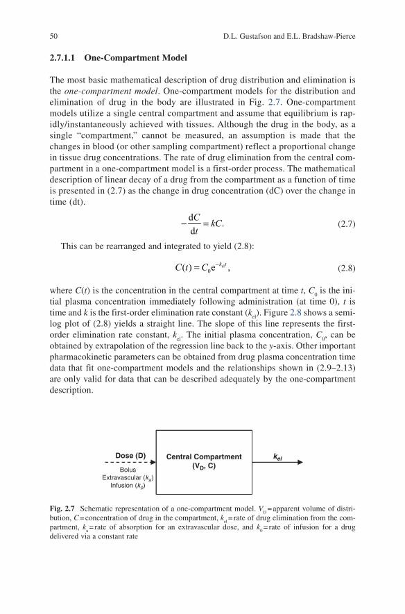
The most basic mathematical description of drug distribution and elimination is the one-compartment model. One-compartment models for the distribution and elimination of drug in the body are illustrated in Fig. 2.7. One-compartment models utilize a single central compartment and assume that equilibrium is rap-idly/instantaneously achieved with tissues. Although the drug in the body, as a single “compartment,” cannot be measured, an assumption is made that the changes in blood (or other sampling compartment) reflect a proportional change in tissue drug concentrations. The rate of drug elimination from the central com-partment in a one-compartment model is a first-order process. The mathematical description of linear decay of a drug from the compartment as a function of time is presented in (2.7) as the change in drug concentration (dC) over the change in time (dt).
d
.d
− =CkC
t (2.7)
This can be rearranged and integrated to yield (2.8):
el0( ) e ,−= k tC t C (2.8)
where C(t) is the concentration in the central compartment at time t, C0 is the ini-
tial plasma concentration immediately following administration (at time 0), t is time and k is the first-order elimination rate constant (k
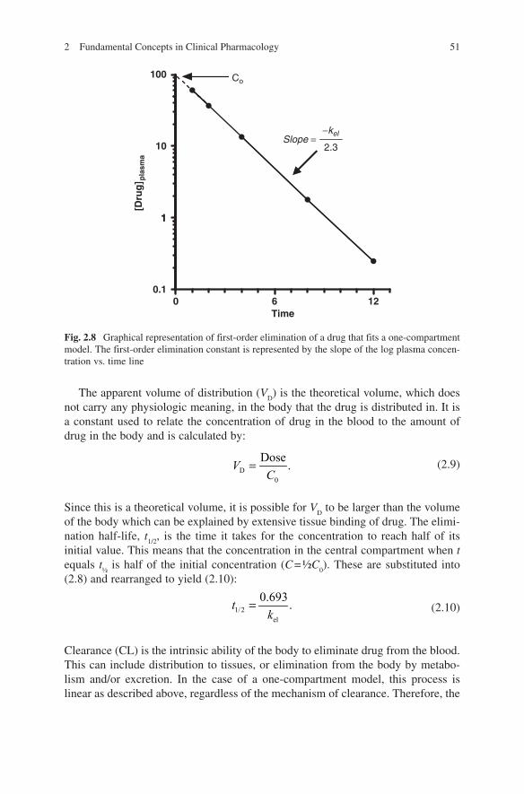
el). Figure 2.8 shows a semi-
log plot of (2.8) yields a straight line. The slope of this line represents the first-order elimination rate constant, k
el. The initial plasma concentration, C
0, can be
obtained by extrapolation of the regression line back to the y-axis. Other important pharmacokinetic parameters can be obtained from drug plasma concentration time data that fit one-compartment models and the relationships shown in (2.9–2.13) are only valid for data that can be described adequately by the one-compartment description.
Central Compartment(VD, C)
Dose (D)
BolusExtravascular (ka)
Infusion (k0)
kel
Fig. 2.7 Schematic representation of a one-compartment model. VD = apparent volume of distri-
bution, C = concentration of drug in the compartment, kel = rate of drug elimination from the com-
partment, ka = rate of absorption for an extravascular dose, and k
0 = rate of infusion for a drug
delivered via a constant rate
512 Fundamental Concepts in Clinical Pharmacology
The apparent volume of distribution (VD) is the theoretical volume, which does
not carry any physiologic meaning, in the body that the drug is distributed in. It is a constant used to relate the concentration of drug in the blood to the amount of drug in the body and is calculated by:
D
0
Dose.=V
C (2.9)
Since this is a theoretical volume, it is possible for VD to be larger than the volume
of the body which can be explained by extensive tissue binding of drug. The elimi-nation half-life, t
1/2, is the time it takes for the concentration to reach half of its
initial value. This means that the concentration in the central compartment when t equals t
½ is half of the initial concentration (C = ½C
0). These are substituted into
(2.8) and rearranged to yield (2.10):
1/2el
0.693.=t
k (2.10)
Clearance (CL) is the intrinsic ability of the body to eliminate drug from the blood. This can include distribution to tissues, or elimination from the body by metabo-lism and/or excretion. In the case of a one-compartment model, this process is linear as described above, regardless of the mechanism of clearance. Therefore, the
100 Co
2.3
−kelSlope =
10
1
[Dru
g] p
lasm
a
1
0 6 120.1
Time
Fig. 2.8 Graphical representation of first-order elimination of a drug that fits a one-compartment model. The first-order elimination constant is represented by the slope of the log plasma concen-tration vs. time line
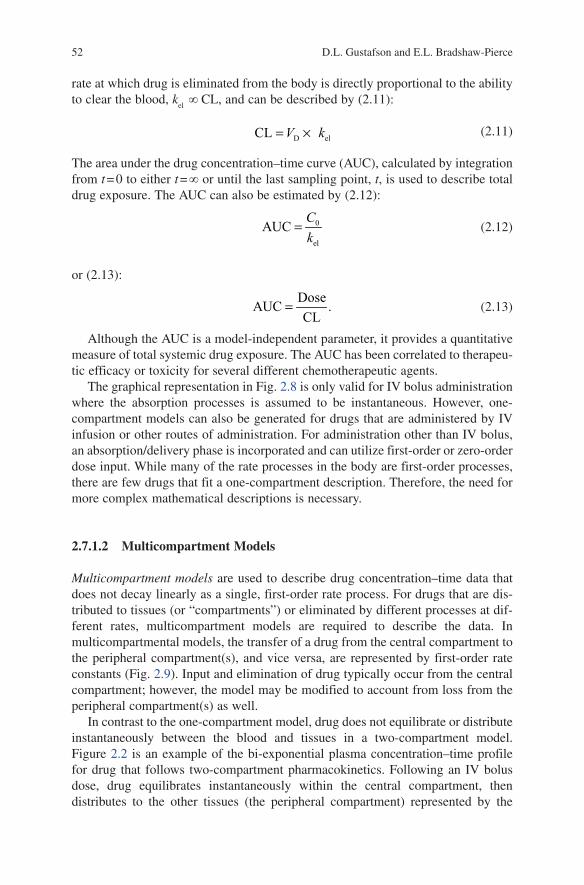
52 D.L. Gustafson and E.L. Bradshaw-Pierce
rate at which drug is eliminated from the body is directly proportional to the ability to clear the blood, k
el ¥ CL, and can be described by (2.11):
D elCL .V k= × (2.11)
The area under the drug concentration–time curve (AUC), calculated by integration from t = 0 to either t = ¥ or until the last sampling point, t, is used to describe total drug exposure. The AUC can also be estimated by (2.12):
0
el
AUC =C
k (2.12)
or (2.13):
Dose
AUC .CL
= (2.13)
Although the AUC is a model-independent parameter, it provides a quantitative measure of total systemic drug exposure. The AUC has been correlated to therapeu-tic efficacy or toxicity for several different chemotherapeutic agents.
The graphical representation in Fig. 2.8 is only valid for IV bolus administration where the absorption processes is assumed to be instantaneous. However, one-compartment models can also be generated for drugs that are administered by IV infusion or other routes of administration. For administration other than IV bolus, an absorption/delivery phase is incorporated and can utilize first-order or zero-order dose input. While many of the rate processes in the body are first-order processes, there are few drugs that fit a one-compartment description. Therefore, the need for more complex mathematical descriptions is necessary.
2.7.1.2 Multicompartment Models
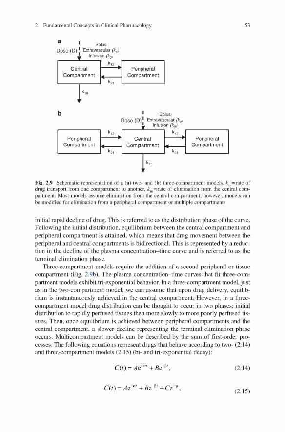
Multicompartment models are used to describe drug concentration–time data that does not decay linearly as a single, first-order rate process. For drugs that are dis-tributed to tissues (or “compartments”) or eliminated by different processes at dif-ferent rates, multicompartment models are required to describe the data. In multicompartmental models, the transfer of a drug from the central compartment to the peripheral compartment(s), and vice versa, are represented by first-order rate constants (Fig. 2.9). Input and elimination of drug typically occur from the central compartment; however, the model may be modified to account from loss from the peripheral compartment(s) as well.
In contrast to the one-compartment model, drug does not equilibrate or distribute instantaneously between the blood and tissues in a two-compartment model. Figure 2.2 is an example of the bi-exponential plasma concentration–time profile for drug that follows two-compartment pharmacokinetics. Following an IV bolus dose, drug equilibrates instantaneously within the central compartment, then distributes to the other tissues (the peripheral compartment) represented by the
532 Fundamental Concepts in Clinical Pharmacology
initial rapid decline of drug. This is referred to as the distribution phase of the curve. Following the initial distribution, equilibrium between the central compartment and peripheral compartment is attained, which means that drug movement between the peripheral and central compartments is bidirectional. This is represented by a reduc-tion in the decline of the plasma concentration–time curve and is referred to as the terminal elimination phase.
Three-compartment models require the addition of a second peripheral or tissue compartment (Fig. 2.9b). The plasma concentration–time curves that fit three-com-partment models exhibit tri-exponential behavior. In a three-compartment model, just as in the two-compartment model, we can assume that upon drug delivery, equilib-rium is instantaneously achieved in the central compartment. However, in a three-compartment model drug distribution can be thought to occur in two phases; initial distribution to rapidly perfused tissues then more slowly to more poorly perfused tis-sues. Then, once equilibrium is achieved between peripheral compartments and the central compartment, a slower decline representing the terminal elimination phase occurs. Multicompartment models can be described by the sum of first-order pro-cesses. The following equations represent drugs that behave according to two- (2.14) and three-compartment models (2.15) (bi- and tri-exponential decay):
( ) e e ,−α −β= +t tC t A B (2.14)
( ) e e e ,−α −β −γ= + +t t tC t A B C (2.15)
CentralCompartment
PeripheralCompartment
k12
BolusExtravascular (ka)
Infusion (k0)
BolusExtravascular (ka)
Infusion (k0)
Dose (D)
a
b
k10
k21
k12
k21
CentralCompartment
PeripheralCompartment
PeripheralCompartment
Dose (D)
k13
pk31
k10
Fig. 2.9 Schematic representation of a (a) two- and (b) three-compartment models. kxy
= rate of drug transport from one compartment to another, k
10 = rate of elimination from the central com-
partment. Most models assume elimination from the central compartment; however, models can be modified for elimination from a peripheral compartment or multiple compartments
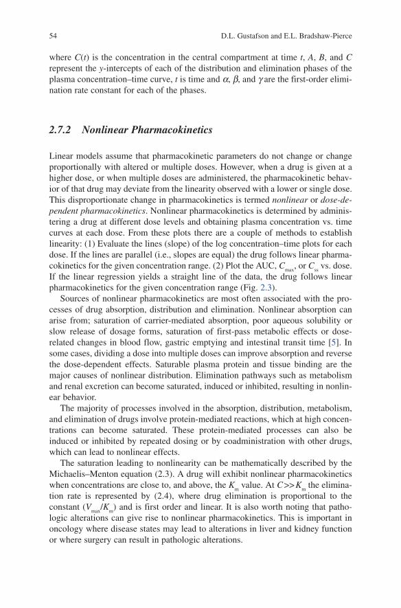
54 D.L. Gustafson and E.L. Bradshaw-Pierce
where C(t) is the concentration in the central compartment at time t, A, B, and C represent the y-intercepts of each of the distribution and elimination phases of the plasma concentration–time curve, t is time and a, b, and g are the first-order elimi-nation rate constant for each of the phases.
2.7.2 Nonlinear Pharmacokinetics
Linear models assume that pharmacokinetic parameters do not change or change proportionally with altered or multiple doses. However, when a drug is given at a higher dose, or when multiple doses are administered, the pharmacokinetic behav-ior of that drug may deviate from the linearity observed with a lower or single dose. This disproportionate change in pharmacokinetics is termed nonlinear or dose-de-pendent pharmacokinetics. Nonlinear pharmacokinetics is determined by adminis-tering a drug at different dose levels and obtaining plasma concentration vs. time curves at each dose. From these plots there are a couple of methods to establish linearity: (1) Evaluate the lines (slope) of the log concentration–time plots for each dose. If the lines are parallel (i.e., slopes are equal) the drug follows linear pharma-cokinetics for the given concentration range. (2) Plot the AUC, C
max, or C
ss vs. dose.
If the linear regression yields a straight line of the data, the drug follows linear pharmacokinetics for the given concentration range (Fig. 2.3).
Sources of nonlinear pharmacokinetics are most often associated with the pro-cesses of drug absorption, distribution and elimination. Nonlinear absorption can arise from; saturation of carrier-mediated absorption, poor aqueous solubility or slow release of dosage forms, saturation of first-pass metabolic effects or dose-related changes in blood flow, gastric emptying and intestinal transit time [5]. In some cases, dividing a dose into multiple doses can improve absorption and reverse the dose-dependent effects. Saturable plasma protein and tissue binding are the major causes of nonlinear distribution. Elimination pathways such as metabolism and renal excretion can become saturated, induced or inhibited, resulting in nonlin-ear behavior.
The majority of processes involved in the absorption, distribution, metabolism, and elimination of drugs involve protein-mediated reactions, which at high concen-trations can become saturated. These protein-mediated processes can also be induced or inhibited by repeated dosing or by coadministration with other drugs, which can lead to nonlinear effects.
The saturation leading to nonlinearity can be mathematically described by the Michaelis–Menton equation (2.3). A drug will exhibit nonlinear pharmacokinetics when concentrations are close to, and above, the K
m value. At C >> K
m the elimina-
tion rate is represented by (2.4), where drug elimination is proportional to the constant (V
max/K
m) and is first order and linear. It is also worth noting that patho-
logic alterations can give rise to nonlinear pharmacokinetics . This is important in oncology where disease states may lead to alterations in liver and kidney function or where surgery can result in pathologic alterations.
552 Fundamental Concepts in Clinical Pharmacology
2.7.3 Noncompartmental Pharmacokinetics
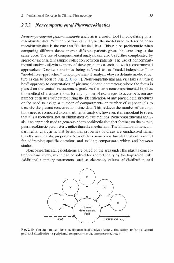
Noncompartmental pharmacokinetic analysis is a useful tool for calculating phar-macokinetic data. With compartmental analysis, the model used to describe phar-macokinetic data is the one that fits the data best. This can be problematic when comparing different doses or even different patients given the same drug at the same dose. The use of compartmental analysis can also be further complicated by sparse or inconsistent sample collection between patients. The use of noncompart-mental analysis alleviates many of these problems associated with compartmental approaches. Despite sometimes being referred to as “model-independent” or “model-free approaches,” noncompartmental analysis obeys a definite model struc-ture as can be seen in Fig. 2.10 [6, 7]. Noncompartmental analysis takes a “black box” approach to computation of pharmacokinetic parameters; where the focus is placed on the central measurement pool. As the term noncompartmental implies, this method of analysis allows for any number of exchanges to occur between any number of tissues without requiring the identification of any physiologic structures or the need to assign a number of compartments or number of exponentials to describe the plasma concentration–time data. This reduces the number of assump-tions needed compared to compartmental analysis; however, it is important to stress that it is a reduction, not an elimination of assumptions. Noncompartmental analy-sis is an approach used to generate pharmacokinetic data that focuses on the output, pharmacokinetic parameters, rather than the mechanism. The limitation of noncom-partmental analysis is that behavioral properties of drugs are emphasized rather than the mechanistic properties. Nevertheless, noncompartmental analysis is useful for addressing specific questions and making comparisons within and between studies.
Noncompartmental calculations are based on the area under the plasma concen-tration–time curve, which can be solved for geometrically by the trapezoidal rule. Additional summary parameters, such as clearance, volume of distribution, and
3
2 4
1 nCentral
MeasurementPool
Input Elimination (k10)
Fig. 2.10 General “model” for noncompartmental analysis representing sampling from a central pool and distribution to peripheral compartments via unrepresented rates
56 D.L. Gustafson and E.L. Bradshaw-Pierce
mean residence time can then be calculated from this. Detailed explanations and derivation of equations for noncompartmental calculations can be found elsewhere [6].
2.7.4 Physiologically Based Pharmacokinetic Models
Physiologically based pharmacokinetic (PBPK) models are more sophisticated pharmacokinetic models that mathematically incorporate principles of physiology, biochemistry, and chemical engineering to model the body as a chemical plant. The fundamental objective of PBPK modeling is to identify the principal organs or tis-sues involved in the disposition of the compound of interest, and to correlate absorption, distribution, and elimination within and among these organs and tissues in an integrated and biologically plausible manner. Compartments in PBPK model-ing, in contrast to classical compartmental modeling, represent specific organs or tissue groups, requiring PBPK models to utilize a large body of physiologic and physio-chemical data. Strengths of PBPK models, compared to classical compart-mental approaches, include the ability to extrapolate between doses, routes of administration and species, and the capability of a priori prediction of plasma and tissue distribution [8].
Due to the complexity of biological systems, several assumptions are imposed in the development of PBPK models, either to simplify the model or as a result of limited data. During the initial development of the model these assumptions include the following: (1) The model is flow limited. This means that organs are well-mixed systems that reach equilibrium with drug concentrations immediately. If tissue uptake studies indicate that the model is not flow limited, diffusion-limited approaches can be incorporated. (2) The concentration of drug in any given com-partment is homogeneous. For well-perfused organs, this is likely to be an accurate assumption. However, for slowly perfused organs such as fat and muscle, this assumption is only a first-order approximation.
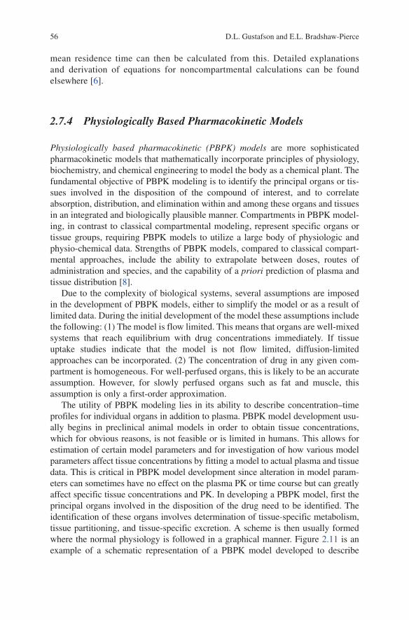
The utility of PBPK modeling lies in its ability to describe concentration–time profiles for individual organs in addition to plasma. PBPK model development usu-ally begins in preclinical animal models in order to obtain tissue concentrations, which for obvious reasons, is not feasible or is limited in humans. This allows for estimation of certain model parameters and for investigation of how various model parameters affect tissue concentrations by fitting a model to actual plasma and tissue data. This is critical in PBPK model development since alteration in model param-eters can sometimes have no effect on the plasma PK or time course but can greatly affect specific tissue concentrations and PK. In developing a PBPK model, first the principal organs involved in the disposition of the drug need to be identified. The identification of these organs involves determination of tissue-specific metabolism, tissue partitioning, and tissue-specific excretion. A scheme is then usually formed where the normal physiology is followed in a graphical manner. Figure 2.11 is an example of a schematic representation of a PBPK model developed to describe
572 Fundamental Concepts in Clinical Pharmacology
plasma and tissue distribution of docetaxel [8]. Within the boundary of an identified compartment (e.g., an organ or tissue or a group of organs or tissues), whatever comes in must be accounted for via leaving, accumulation, or elimination from the compartment. The resulting “mass balance” is expressed as a mathematical equation with appropriate parameters carrying biological significance. An example of mass balance within a tissue compartment is given by (2.16):
vii ii a
i
d( ) ,
d
×= × − −
CV CQ C X
t P (2.16)
where, Vi = the volume of the compartment (organ or group of organs), C
i = con-
centration of drug in the compartment, Qi = blood flow to the compartment,
Ca = concentration of drug in arterial blood, C
vi = drug concentration in venous
blood leaving compartment i, Pi = tissue:blood partitioning of the drug for that
compartment, and X = clearance term (metabolism, excretion). The differential mass balance equations for all compartments are solved simultaneously, which in turn is used for computer simulations predicting the time course for any given
QSP, CACVSP Slowly Perfused
PSP VSP
Rapidly Perfused
PRP VRP
QRP, CACVRP
Kidney
PK VK
QK, CACVK
Gut
PG VG
Liver
PL VLQG, CA
QL, CA
QG, CVG
CVL
Urinary Excretion Fecal Excretion
VmaxB KmB VmaxI KmI
VmaxLM KmLM
VmaxAS KmAS
Metabolism tot-OH-butyl-docetaxel
Fig. 2.11 Schematic representation of a PBPK model for docetaxel disposition (reprinted from [8])
58 D.L. Gustafson and E.L. Bradshaw-Pierce
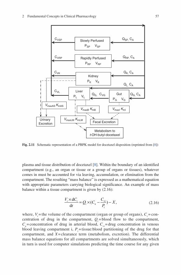
parameter. In principle, if all the parameters that can affect the drug disposition are accounted for, the model should be capable of predicting what takes place in vivo. Figure 2.12 illustrates the ability of PBPK models to accurately
1000
10000
100000
1000
10000
Plasma Plasma
Mouse20 mg/kg 5 mg/kg
10
100
Do
ceta
xel [
nm
ol/L
]D
oce
taxe
l [n
mo
l/L]
Do
ceta
xel [
nm
ol/L
]
Do
ceta
xel [
nm
ol/L
]D
oce
taxe
l [n
mo
l/L]
Do
ceta
xel [
nm
ol/L
]
1000
10000
100000
10
100
1000
10000
Liver Liver
100 100
100
1000
10000
100000
100
1000
10000
Intestine Intestine
0 4 8 12 16 20 24Time [h]
0 4 8 12Time [h]
Do
ceta
xel [
nm
ol/L
]
1000
Human
0 10 20 30 40 501
10
100
1000
1
10
100
1000
1
10
100
Time (h)0 10 20 30 40 50
Time (h)0 10 20 30 40 50
Time (h)
Fig. 2.12 PBPK model developed for prediction of docetaxel plasma and tissue distribution in mice and humans. This PBPK model was able to accurately predict the plasma and tissue distribution in mice following IV bolus administration at two different doses (20 and 5 mg/kg). The model was then scaled to human organ, blood flow, tissue binding, metabolic and excretory parameters, and doc-etaxel plasma levels accurately predicted (36 mg/m2 by IV infusion). Symbols represent actual data points and the solid lines represent the PBPK model simulations (figure modified from [8])
592 Fundamental Concepts in Clinical Pharmacology
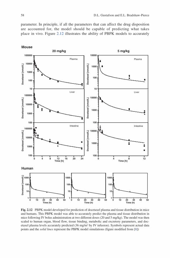
predict plasma and tissue concentrations at different doses and the ability to extrapolate between species. It is important to note that the PBPK model simulations, represented by solid lines, exist without the data. In other words, the lines do not represent a “fit” to the data, rather data itself generated by the model. Figure 2.13 shows plasma concentration–time curves for docetaxel administered at different doses though different routes of administration predicted by a PBPK model. This illustrates the potential utility of PBPK models to aid in the advancement of “model-directed” experimental design of combination therapies and/or alternate dosing schedules. The value of PBPK models expands beyond preclinical research. In fact, PBPK models have been developed for several clinically used chemotherapeutic agents such as: docetaxel [8], adriamycin [9], ara-C [10], cisplatin [11], methotrexate [12], and capecitabine/5-FU [13].
PBPK models have the ability to be coupled to Monte Carlo simulation, which can then account for variability across model parameters such as induction of CYP3A activity or reduction of CYP3A activity due to impaired liver function or competitive inhibition by a coadministered drug. In fact, a PBPK model of doxorubicin was coupled to Monte Carlo simulation to predict the interaction of paclitaxel on doxorubicin pharmacokinetics [14]. This study showed that paclitaxel did not affect plasma pharmacokinetic of doxorubicin but did affect tissue pharmacokinetics. This information would not have been revealed by simple compartmental or noncompartmental modeling of the doxorubicin plasma concentration–time data.
3mg/kg IV 6 mg/kg IP 1 mg/kg IP9 mg/kg IV
100
1000
10
Do
ceta
xel [
nM
]
0 1 2 3 4 5 6 7 8 9 100.1
1
Time (days)
Fig. 2.13 Examples of PBPK model simulations of docetaxel plasma concentrations in mice with differing doses, routes of administration, and schedules
60 D.L. Gustafson and E.L. Bradshaw-Pierce
2.7.5 Population Pharmacokinetics
Population pharmacokinetics is the process by which individual characteristics within a population are utilized to try and identify sources of variability that can potentially be accounted for in drug dosing decisions. Thus, it is a useful tool for identifying the sources of pharmacokinetic variability and can aid in the design of alternative dosing regimens to enhance drug efficacy and safety. The foundations of population PK modeling were laid in the 1970s by Sheiner et al. [15, 16], who showed that population PK modeling can estimate the average values of PK param-eters and the interindividual variances of those parameters in a patient population. In addition to measuring interindividual variances, population PK can also account for some of this variability in terms of patient differences in genetic, physiological, pathological, and/or environmental factors. Thus, population-based methods facili-tate the development of individualized dosing regimens based on patient-specific covariates. For example, should a drug be dosed based on the body weight of the patient (per kg) or per body surface area (BSA)? The question can be answered by taking body weight and body surface area into consideration when analyzing the pharmacokinetic data from a population, and determine the degree of dependence of specific pharmacokinetic parameters to these factors.
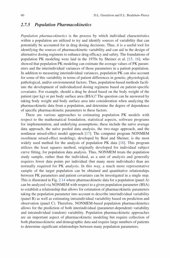
There are various approaches to estimating population PK models with respect to the mathematical foundation, statistical aspects, software programs for implementation, and underlying assumptions; these include the naïve average data approach, the naïve pooled data analysis, the two-stage approach, and the nonlinear mixed-effect model approach [17]. The computer program NONMEM (nonlinear mixed-effect modeling), developed by Beal and Sheiner, is the most widely used method for the analysis of population PK data [18]. This program utilizes the least squares method, originally developed for individual subject curve fitting, for population data analysis. Thus, NONMEM treats the population study sample, rather than the individual, as a unit of analysis and generally requires fewer data points per individual (but many more individuals) than are normally required for PK analysis. In this way, a much more representative sample of the target population can be obtained and quantitative relationships between PK parameters and patient covariates can be investigated in a single step. This is illustrated in Fig. 2.14 where pharmacokinetic data for a population (panel A) can be analyzed via NONMEM with respect to a given population parameter (BSA) to establish a relationship that allows for estimation of pharmacokinetic parameters taking the population parameter into account to describe interindividual variability (panel B) as well as estimating intraindividual variability based on prediction and observation (panel C). Therefore, NONMEM-based population pharmacokinetics allows for the prediction of both interindividual (parameter-dependent) variability and intraindividual (random) variability. Population pharmacokinetic approaches are an important aspect of pharmacokinetic modeling but require collection of both pharmacokinetic and demographic data and require large numbers of patients to determine significant relationships between many population parameters.
612 Fundamental Concepts in Clinical Pharmacology
References
1. Perry S. Reduction of toxicity in cancer chemotherapy. Cancer Res 1969; 29: 2319–25. 2. Thomas SM, Grandis JR. Pharmacokinetic and pharmacodynamic properties of EGFR inhibi-
tors under clinical investigation. Cancer Treat Rev 2004; 30: 255–68. 3. Gustafson DL, Long ME, Zirrolli JA, et al. Analysis of docetaxel pharmacokinetics in humans
with the inclusion of later sampling time points afforded by the use of a sensitive tandem LCMS assay. Cancer Chemother Pharmacol 2003; 52: 159–66.
4. Stowe CM, Plaa GL. Extrarenal excretion of drugs and chemicals. Annu Rev Pharmacol 1968; 8: 337–56.
5. Ludden TM. Nonlinear pharmacokinetics: clinical implications. Clin Pharmacokinet 1991; 20: 429–46.
6. Wagner JG. Noncompartmental and System Analysis. Pharmacokinetics for the Pharmaceutical Scientist. Lancaster, PA: Technomic Publishing Company; 1993. p. 83–99.
7. DiStefano JJ, III. Noncompartmental vs. compartmental analysis: some bases for choice. Am J Physiol Regul Integr Comp Physiol 1982; 243: R1–6.
8. Bradshaw-Pierce EL, Eckhardt SG, Gustafson DL. A physiologically-based phar-macokinetic model of docetaxel disposition: from mouse to man. Clin Cancer Res 2007; 13: 2768–76.
9. Gustafson DL, Rastatter JC, Colombo T, Long ME. Doxorubicin pharmacokinetics: macro-molecule binding, metabolism and elimination in the context of a physiological model. J Pharm Sci 2002; 91: 1488–501.
Fig. 2.14 Nonlinear mixed effects modeling (NONMEM) simultaneous estimation of parameters relating fixed effects and random effects to observed data for population pharmacokinetic modeling
62 D.L. Gustafson and E.L. Bradshaw-Pierce
10. Dedrick RL, Forrester DD, Cannon JN, El Dareer SM, Mellett LB. Pharmacokinetics of 1-d-arabinofuranosylcytosine (Ara-C) deamination in several species. Biochem Pharmacol 1973; 22: 2405–17.
11. Farris FF, King FG, Dedrick RL, Litterst CL. Physiological model for the pharmacokinetics of cis-dichlorodiammineplatinum (II) (DDP) in the tumored rat. J Pharmacokinet Biopharm 1985; 13: 13–39.
12. Bischoff KB, Dedrick RL, Zaharko DS, Longstreth JA. Methotrexate pharmacokinetics. J Pharm Sci 1971; 60: 1128–33.
13. Tsukamoto Y, Kato Y, Ura M, Horii I, Ishikawa T, Ishitsuka H, Sugiyama Y. Investigation of 5-FU disposition after oral administration of capecitabine, a triple-prodrug of 5-FU, using a physiologically based pharmacokinetic model in a human cancer xenograft model: compari-son of the simulated 5-FU exposures in the tumour tissue between human and xenograft model. Biopharm Drug Dispos 2001; 22: 1–14.
14. Gustafson DL. Use of physiologically-based pharmacokinetic modeling coupled to Monte Carlo simulation to predict the pharmacokinetic interactions between doxorubicin and taxanes in human populations. Proc Am Assoc Cancer Res 2002; 43: 208.
15. Sheiner LB, Rosenberg B, Marathe VV. Estimation of population characteristics of pharma-cokinetic parameters from routine clinical data. J Pharmacokinet Biopharm 1977; 5: 445–79.
16. Sheiner LB, Rosenberg B, Melmon KL. Modelling of individual pharmacokinetics for computer-aided drug dosage. Comput Biomed Res 1972; 5: 411–59.
17. Ette EI, Williams PJ. Population pharmacokinetics II: estimation methods. Ann Pharmacother 2004; 38: 1907–15.
18. Aarons L. Population pharmacokinetics: theory and practice. Br J Clin Pharmacol 1991; 32: 669–70.
http://www.springer.com/978-1-4419-7357-3