Multi-SensorData Fusion

withMATLAB®

CRC Press is an imprint of theTaylor & Francis Group, an informa business

Boca Raton London New York

Jitendra R. Raol

Multi-SensorData Fusion

withMATLAB®

MATLAB® and Simulink® are trademarks of The MathWorks, Inc. and are used with permission. The MathWorks does not warrant the accuracy of the text of exercises in this book. This book’s use or dis -cussion of MATLAB® and Simulink® software or related products does not constitute endorsement or sponsorship by The MathWorks of a particular pedagogical approach or particular use of the MATLAB® and Simulink® software.

CRC PressTaylor & Francis Group6000 Broken Sound Parkway NW, Suite 300Boca Raton, FL 33487-2742

© 2010 by Taylor and Francis Group, LLCCRC Press is an imprint of Taylor & Francis Group, an Informa business

No claim to original U.S. Government works

Printed in the United States of America on acid-free paper10 9 8 7 6 5 4 3 2 1

International Standard Book Number: 978-1-4398-0003-4 (Hardback)

This book contains information obtained from authentic and highly regarded sources. Reasonable efforts have been made to publish reliable data and information, but the author and publisher cannot assume responsibility for the validity of all materials or the consequences of their use. The authors and publishers have attempted to trace the copyright holders of all material reproduced in this publication and apologize to copyright holders if permission to publish in this form has not been obtained. If any copyright material has not been acknowledged please write and let us know so we may rectify in any future reprint.

Except as permitted under U.S. Copyright Law, no part of this book may be reprinted, reproduced, trans-mitted, or utilized in any form by any electronic, mechanical, or other means, now known or hereafter invented, including photocopying, microfilming, and recording, or in any information storage or retrieval system, without written permission from the publishers.

For permission to photocopy or use material electronically from this work, please access www.copyright.com (http://www.copyright.com/) or contact the Copyright Clearance Center, Inc. (CCC), 222 Rosewood Drive, Danvers, MA 01923, 978-750-8400. CCC is a not-for-profit organization that provides licenses and registration for a variety of users. For organizations that have been granted a photocopy license by the CCC, a separate system of payment has been arranged.

Trademark Notice: Product or corporate names may be trademarks or registered trademarks, and are used only for identification and explanation without intent to infringe.

Library of Congress Cataloging-in-Publication Data

Raol, J. R. (Jitendra R.), 1947-Multi-sensor data fusion with MATLAB / Jitendra R. Raol.

p. cm.“A CRC title.”Includes bibliographical references and index.ISBN 978-1-4398-0003-4 (hardcover : alk. paper)1. Multisensor data fusion— Data processing. 2. MATLAB. 3. Detectors. I. Title.

TA331.R36 2010681’.2—dc22 2009041607

Visit the Taylor & Francis Web site athttp://www.taylorandfrancis.com

and the CRC Press Web site athttp://www.crcpress.com

The book is dedicated

in loving memory to

Professor P. N. Thakre

(M. S. University of Baroda, Vadodara),

Professor Vimal K. Dubey

(Nanyang Technological University, Singapore),

and

Professor Vinod J. Modi

(University of British Columbia, Canada)

vii

Contents

Preface ................................................................................................... xix Acknowledgments ................................................................................ xxi Author .................................................................................................xxiii Contributors ......................................................................................... xxv Introduction .......................................................................................xxvii

I: Theory of Data Fusion and Kinematic-Level Fusion Part (J. R. Raol, G. Girija, and N. Shanthakumar)

1. Introduction .................................................................................................. 3

2. Concepts and Theory of Data Fusion ..................................................... 11 2.1 Models of the Data Fusion Process and Architectures ..................... 11

2.1.1 Data Fusion Models .................................................................... 132.1.1.1 Joint Directors of Laboratories Model ....................... 132.1.1.2 Modifi ed Waterfall Fusion Model .............................. 172.1.1.3 Intelligence Cycle–Based Model ................................ 182.1.1.4 Boyd Model ................................................................... 192.1.1.5 Omnibus Model ........................................................... 20

2.1.2 Fusion Architectures .................................................................. 212.1.2.1 Centralized Fusion ....................................................... 212.1.2.2 Distributed Fusion ....................................................... 212.1.2.3 Hybrid Fusion ............................................................... 22

2.2 Unifi ed Estimation Fusion Models and Other Methods ................... 232.2.1 Defi nition of the Estimation Fusion Process ........................... 242.2.2 Unifi ed Fusion Models Methodology ...................................... 25

2.2.2.1 Special Cases of the Unifi ed Fusion Models ............ 252.2.2.2 Correlation in the Unifi ed Fusion Models ................ 26

2.2.3 Unifi ed Optimal Fusion Rules .................................................. 272.2.3.1 Best Linear Unbiased Estimation Fusion Rules

with Complete Prior Knowledge ............................... 272.2.3.2 Best Linear Unbiased Estimation Fusion Rules

without Prior Knowledge ........................................... 282.2.3.3 Best Linear Unbiased Estimation Fusion Rules

with Incomplete Prior Knowledge ............................ 282.2.3.4 Optimal-Weighted Least Squares Fusion Rule ........ 282.2.3.5 Optimal Generalized Weighted Least Squares

Fusion Rule ................................................................... 29

viii Contents

2.2.4 Kalman Filter Technique as a Data Fuser ............................... 292.2.4.1 Data Update Algorithm............................................... 302.2.4.2 State-Propagation Algorithm ..................................... 31

2.2.5 Inference Methods ...................................................................... 322.2.6 Perception, Sensing, and Fusion ............................................... 32

2.3 Bayesian and Dempster–Shafer Fusion Methods .............................. 332.3.1 Bayesian Method ......................................................................... 34

2.3.1.1 Bayesian Method for Fusion of Data from Two Sensors .................................................................. 36

2.3.2 Dempster–Shafer Method ......................................................... 382.3.3 Comparison of the Bayesian Inference Method and

the Dempster–Shafer Method ................................................... 402.4 Entropy-Based Sensor Data Fusion Approach ................................... 41

2.4.1 Defi nition of Information .......................................................... 412.4.2 Mutual Information .................................................................... 432.4.3 Entropy in the Context of an Image ......................................... 442.4.4 Image-Noise Index ...................................................................... 44

2.5 Sensor Modeling, Sensor Management, and Information Pooling ..... 452.5.1 Sensor Types and Classifi cation ............................................... 45

2.5.1.1 Sensor Technology ....................................................... 462.5.1.2 Other Sensors and their Important Features

and Usages .................................................................... 482.5.1.3 Features of Sensors ...................................................... 512.5.1.4 Sensor Characteristics ............................................... 52

2.5.2 Sensor Management ................................................................... 532.5.2.1 Sensor Modeling .......................................................... 552.5.2.2 Bayesian Network Model ............................................ 582.5.2.3 Situation Assessment Process .................................... 58

2.5.3 Information-Pooling Methods .................................................. 602.5.3.1 Linear Opinion Pool .................................................... 602.5.3.2 Independent Opinion Pool ......................................... 612.5.3.3 Independent Likelihood Pool ..................................... 61

3. Strategies and Algorithms for Target Tracking and Data Fusion ........................................................................................................... 63

3.1 State-Vector and Measurement-Level Fusion ..................................... 693.1.1 State-Vector Fusion ..................................................................... 703.1.2 Measurement Data–Level Fusion ............................................. 713.1.3 Results with Simulated and Real Data Trajectories ............... 713.1.4 Results for Data from a Remote Sensing Agency with

Measurement Data–Level Fusion ............................................. 723.2 Factorization Kalman Filters for Sensor Data Characterization

and Fusion ................................................................................................ 733.2.1 Sensor Bias Errors ....................................................................... 73

Contents ix

3.2.2 Error State-Space Kalman Filter ............................................... 753.2.3 Measurement and Process Noise Covariance

Estimation .................................................................................... 763.2.4 Time Stamp and Time Delay Errors ......................................... 773.2.5 Multisensor Data Fusion Scheme ............................................. 77

3.2.5.1 UD Filters for Trajectory Estimation ......................... 803.2.5.2 Measurement Fusion ................................................... 813.2.5.3 State-Vector Fusion ....................................................... 823.2.5.4 Fusion Philosophy ........................................................ 82

3.3 Square-Root Information Filtering and Fusion in Decentralized Architecture ................................................................... 863.3.1 Information Filter ........................................................................ 87

3.3.1.1 Information Filter Concept ......................................... 873.3.1.2 Square Root Information Filter Algorithm .............. 88

3.3.2 Square Root Information Filter Sensor Data Fusion Algorithm ..................................................................................... 88

3.3.3 Decentralized Square Root Information Filter ....................... 893.3.4 Numerical Simulation Results .................................................. 91

3.4 Nearest Neighbor and Probabilistic Data Association Filter Algorithms ............................................................................................... 933.4.1 Nearest Neighborhood Kalman Filter ..................................... 943.4.2 Probabilistic Data Association Filter ........................................ 963.4.3 Tracking and Data Association Program for

Multisensor, Multitarget Sensors ............................................. 973.4.3.1 Sensor Attributes.......................................................... 993.4.3.2 Data Set Conversion ..................................................... 993.4.3.3 Gating in Multisensor, Multitarget .......................... 1003.4.3.4 Measurement-to-Track Association ......................... 1003.4.3.5 Initiation of Track and Extrapolation of Track ....... 1013.4.3.6 Extrapolation of Tracks into Next Sensor Field

of View ......................................................................... 1013.4.3.7 Extrapolation of Tracks into Next Scan ................... 1023.4.3.8 Track Management Process ...................................... 102

3.4.4 Numerical Simulation .............................................................. 1033.5 Interacting Multiple Model Algorithm for Maneuvering

Target Tracking ..................................................................................... 1063.5.1 Interacting Multiple Model Kalman Filter Algorithm ........ 106

3.5.1.1 Interaction and Mixing ............................................. 1083.5.1.2 Kalman Filtering ........................................................ 1083.5.1.3 Mode Probability Update .......................................... 1093.5.1.4 State Estimate and Covariance Combiner .............. 109

3.5.2 Target Motion Models ...............................................................1103.5.2.1 Constant Velocity Model ............................................1103.5.2.2 Constant Acceleration Model ....................................110

x Contents

3.5.3 Interacting Multiple Model Kalman Filter Implementation ..........................................................................1113.5.3.1 Validation with Simulated Data ............................... 112

3.6 Joint Probabilistic Data Association Filter ..........................................1163.6.1 General Version of a Joint Probabilistic Data

Association Filter .......................................................................1173.6.2 Particle Filter Sample–Based Joint Probabilistic Data

Association Filter .......................................................................1193.7 Out-of-Sequence Measurement Processing for Tracking ................ 120

3.7.1 Bayesian Approach to the Out-of-Sequence Measurement Problem ............................................................. 120

3.7.2 Out-of-Sequence Measurement with Single Delay and No Clutter .................................................................................. 1213.7.2.1 Y Algorithm ................................................................ 1213.7.2.2 Augmented State Kalman Filters ............................. 122

3.8 Data Sharing and Gain Fusion Algorithm for Fusion ..................... 1243.8.1 Kalman Filter–Based Fusion Algorithm ................................ 1243.8.2 Gain Fusion–Based Algorithm ............................................... 1253.8.3 Performance Evaluation ........................................................... 126

3.9 Global Fusion and H-Infi nity Filter–Based Data Fusion ................. 1273.9.1 Sensor Data Fusion using H-Infi nity Filters ......................... 1273.9.2 H-Infi nity a Posteriori Filter–Based Fusion

Algorithm ................................................................................... 1303.9.3 H-Infi nity Global Fusion Algorithm ...................................... 1313.9.4 Numerical Simulation Results ................................................ 132

3.10 Derivative-Free Kalman Filters for Fusion ........................................ 1343.10.1 Derivative-Free Kalman Filters ............................................... 1363.10.2 Numerical Simulation .............................................................. 137

3.10.2.1 Initialization of the Data Fusion-Derivative Free Kalman Filter Algorithm .................................. 140

3.10.2.2 Computation of the Sigma Points ............................ 1403.10.2.3 State and Covariance Propagation............................1413.10.2.4 State and Covariance Update ....................................141

3.11 Missile Seeker Estimator ...................................................................... 1433.11.1 Interacting Multiple Model–Augmented Extended

Kalman Filter Algorithm ......................................................... 1433.11.1.1 State Model .................................................................. 1443.11.1.2 Measurement Model .................................................. 145

3.11.2 Interceptor–Evader Engagement Simulation ........................ 1463.11.2.1 Evader Data Simulation............................................. 147

3.11.3 Performance Evaluation of Interacting Multiple Model–Augmented Extended Kalman Filter ............................................................................. 147

3.12 Illustrative Examples ............................................................................ 151

Contents xi

4. Performance Evaluation of Data Fusion Systems, Software, and Tracking........................................................................... 157

4.1 Real-Time Flight Safety Expert System Strategy .............................. 1604.1.1 Autodecision Criteria ................................................................1614.1.2 Objective of a Flight Test Range ..............................................1614.1.3 Scenario of the Test Range ........................................................161

4.1.3.1 Tracking Instruments .................................................1624.1.3.2 Data Acquisition ......................................................... 1634.1.3.3 Decision Display System ........................................... 163

4.1.4 Multisensor Data Fusion System ............................................ 1634.1.4.1 Sensor Fusion for Range Safety Computer ............ 1644.1.4.2 Algorithms for Fusion ............................................... 1644.1.4.3 Decision Fusion .......................................................... 165

4.2 Multisensor Single-Target Tracking ................................................... 1664.2.1 Hierarchical Multisensor Data Fusion Architecture and

Fusion Scheme ........................................................................... 1664.2.2 Philosophy of Sensor Fusion ................................................... 1684.2.3 Data Fusion Software Structure ............................................. 169

4.2.3.1 Fusion Module 1 ......................................................... 1694.2.3.2 Fusion Modules 2 and 3 ............................................ 169

4.2.4 Validation ................................................................................... 1704.3 Tracking of a Maneuvering Target—Multiple-Target

Tracking Using Interacting Multiple Model Probability Data Association Filter and Fusion .............................................................. 1714.3.1 Interacting Multiple Model Algorithm .................................. 171

4.3.1.1 Automatic Track Formation ...................................... 1714.3.1.2 Gating and Data Association.................................... 1724.3.1.3 Interaction and Mixing in Interactive Multiple

Model Probabilistic Data Association Filter ........... 1744.3.1.4 Mode-Conditioned Filtering.................................... 1744.3.1.5 Probability Computations ......................................... 1754.3.1.6 Combined State and Covariance Prediction

and Estimation ........................................................... 1764.3.2 Simulation Validation ............................................................... 177

4.3.2.1 Constant Velocity Model ........................................... 1774.3.2.2 Constant Acceleration Model ................................... 1784.3.2.3 Performance Evaluation and Discussions .............. 179

4.4 Evaluation of Converted Measurement and Modifi ed Extended Kalman Filters ..................................................................... 1834.4.1 Error Model Converted Measurement Kalman Filter

and Error Model Modifi ed Extended Kalman Filter Algorithms ................................................................................. 1844.4.1.1 Error Model Converted Measurement Kalman

Filter Algorithm .......................................................... 185

xii Contents

4.4.1.2 Error Model Modifi ed Extended Kalman Filter Algorithm .................................................................... 186

4.4.2 Discussion of Results ................................................................ 1894.4.2.1 Sensitivity Study on Error Model Modifi ed

Extended Kalman Filter ............................................ 1914.4.2.2 Comparison of Debiased Converted

Measurements Kalman Filter, Error Model Converted Measurement Kalman Filter, and Error Model Modifi ed Extended Kalman Filter Algorithms .................................................................. 191

4.5 Estimation of Attitude Using Low-Cost Inertial Platforms and Kalman Filter Fusion ............................................................................ 1934.5.1 Hardware System ...................................................................... 1954.5.2 Sensor Modeling ....................................................................... 195

4.5.2.1 Misalignment Error Model ....................................... 1964.5.2.2 Temperature Drift Model .......................................... 1964.5.2.3 CG Offset Model ........................................................ 196

4.5.3 MATLAB®/Simulink Implementation ................................... 1964.5.3.1 State Model .................................................................. 1974.5.3.2 Measurement Model .................................................. 198

4.5.4 Microcontroller Implementation ............................................ 200Epilogue ........................................................................................................... 203Exercises .......................................................................................................... 203References ........................................................................................................ 206

II: Fuzzy Logic and Decision Fusion Part (J. R. Raol and S. K. Kashyap)

5. Introduction .............................................................................................. 215

6. Theory of Fuzzy Logic ............................................................................ 217 6.1 Interpretation and Unifi cation of Fuzzy Logic Operations ............ 218

6.1.1 Fuzzy Sets and Membership Functions ................................ 2186.1.2 Types of Fuzzy Membership Functions ................................ 220

6.1.2.1 Sigmoid-Shaped Function ......................................... 2206.1.2.2 Gaussian-Shaped Function ....................................... 2206.1.2.3 Triangle-Shaped Function ........................................ 2226.1.2.4 Trapezoid-Shaped Function...................................... 2226.1.2.5 S-Shaped Function ..................................................... 2226.1.2.6 Π-Shaped Function .................................................... 2246.1.2.7 Z-Shaped Function..................................................... 224

6.1.3 Fuzzy Set Operations ............................................................... 2256.1.3.1 Fuzzy Logic Operators .............................................. 226

Contents xiii

6.1.4 Fuzzy Inference System ........................................................... 2276.1.4.1 Triangular Norm or T-norm ..................................... 2286.1.4.2 Fuzzy Implication Process Using T-norm .............. 2326.1.4.3 Triangular Conorm or S-norm ................................. 2396.1.4.4 Fuzzy Inference Process Using S-norm .................. 240

6.1.5 Relationships between Fuzzy Logic Operators .................... 2476.1.6 Sup (max)–Star (T-norm) Composition .................................. 248

6.1.6.1 Maximum–Minimum Composition (Mamdani) ................................................................... 249

6.1.6.2 Maximum Product Composition (Larsen) ............. 2506.1.7 Interpretation of the Connective “and” .................................. 2506.1.8 Defuzzifi cation .......................................................................... 251

6.1.8.1 Centroid Method, or Center of Gravity or Center of Area ............................................................. 251

6.1.8.2 Maximum Decomposition Method ......................... 2526.1.8.3 Center of Maxima or Mean of Maximum............... 2526.1.8.4 Smallest of Maximum ............................................... 2536.1.8.5 Largest of Maximum ................................................. 2536.1.8.6 Height Defuzzifi cation .............................................. 253

6.1.9 Steps of the Fuzzy Inference Process ..................................... 2536.2 Fuzzy Implication Functions .............................................................. 255

6.2.1 Fuzzy Implication Methods .................................................... 2556.2.2 Comparative Evaluation of the Various Fuzzy

Implication Methods s with Numerical Data ....................... 2646.2.3 Properties of Fuzzy If-Then Rule Interpretations ................ 265

6.3 Forward- and Backward-Chain Logic Criteria ................................ 2666.3.1 Generalization of Modus Ponens Rule .................................... 2666.3.2 Generalization of Modus Tollens Rule ..................................... 267

6.4 Tool for the Evaluation of Fuzzy Implication Functions ................. 2686.4.1 Study of Criteria Satisfaction Using MATLAB®

Graphics ..................................................................................... 2686.5 Development of New Implication Functions .................................... 275

6.5.1 Study of Criteria Satisfaction by New Implication Function Using MATLAB and GUI Tools ............................. 278

6.6 Fuzzy Logic Algorithms and Final Composition Operations .............................................................................................. 281

6.7 Fuzzy Logic and Fuzzy Integrals in Multiple Network Fusion ..................................................................................................... 289

7. Decision Fusion ........................................................................................ 293 7.1 Symbol- or Decision-Level Fusion ...................................................... 2937.2 Soft Decisions in Kalman Filtering .................................................... 2967.3 Fuzzy Logic–Based Kalman Filter and Fusion Filters ..................... 297

7.3.1 Fuzzy Logic–Based Process and Design ............................... 298

xiv Contents

7.3.2 Comparison of Kalman Filter and Fuzzy Kalman Filter ............................................................................. 299

7.3.3 Comparison of Kalman Filter and Fuzzy Kalman Filter for Maneuvering Target Tracking ................................ 3017.3.3.1 Training Set and Check-Set Data ............................. 3017.3.3.2 Mild and Evasive Maneuver Data ........................... 302

7.3.4 Fuzzy Logic–Based Sensor Data Fusion ................................ 3037.3.4.1 Kalman Filter Fuzzifi cation ...................................... 3047.3.4.2 Fuzzy Kalman Filter Fuzzifi cation .......................... 3067.3.4.3 Numerical Simulation Results ................................. 307

7.4 Fuzzy Logic in Decision Fusion .......................................................... 3087.4.1 Methods Available to Perform Situation

Assessments ................................................................................3107.4.2 Comparison between Bayesian Network

and Fuzzy Logic ........................................................................ 3107.4.2.1 Situation Assessment Using Fuzzy Logic ...............311

7.4.3 Level-3 Threat Refi nement and Level-4 Process Refi nement ................................................................................. 312

7.4.4 Fuzzy Logic–Based Decision Fusion Systems ...................... 3137.4.4.1 Various Attributes and Aspects of Fuzzy

Logic–Based Decision Fusion Systems ....................3147.5 Fuzzy Logic Bayesian Network for Situation Assessment ..............316

7.5.1 Description of Situation Assessment in Air Combat ........... 3177.5.1.1 Exercise Controller ..................................................... 3177.5.1.2 Integrated Sensor Model ............................................3187.5.1.3 Data Processor .............................................................3187.5.1.4 Pilot Mental Model .....................................................318

7.5.2 Bayesian Mental Model .............................................................3187.5.2.1 Pair Agent Bayesian Network .................................. 3197.5.2.2 Along Agent Bayesian Network .............................. 3207.5.2.3 Attack Agent Bayesian Network .............................. 320

7.5.3 Results and Discussions .......................................................... 3207.6 Fuzzy Logic–Based Decision Fusion in a Biometric System .......... 321

7.6.1 Fusion in Biometric Systems ................................................... 3227.6.2 Fuzzy Logic Fusion ................................................................... 322

8. Performance Evaluation of Fuzzy Logic–Based Decision Systems ........................................................................................................ 325

8.1 Evaluation of Existing Fuzzy Implication Functions ...................... 3258.2 Decision Fusion System 1—Formation Flight ................................... 328

8.2.1 Membership Functions ............................................................ 3298.2.2 Fuzzy Rules and the Fuzzy Implication Method ................. 3308.2.3 Aggregation and Defuzzifi cation Method ............................ 3308.2.4 Fuzzy Logic–Based Decision Software Realization ............ 330

Contents xv

8.3 Decision Fusion System 2—Air Lane ................................................. 3318.3.1 Membership Functions ............................................................ 3328.3.2 Fuzzy Rules and Other Methods ............................................ 3338.3.3 Fuzzy Logic–Based Decision Software

Realization for System 2 ........................................................... 3348.4 Evaluation of Some New Fuzzy Implication Functions .................. 3348.5 Illustrative Examples ............................................................................ 337Epilogue ........................................................................................................... 347Exercises .......................................................................................................... 347References ........................................................................................................ 351

III: Pixel- and Feature-Level Image Fusion Part (J. R. Raol and V. P. S. Naidu)

9. Introduction ............................................................................................ 357

10. Pixel- and Feature-Level Image Fusion Concepts and Algorithms .............................................................................................. 361

10.1 Image Registration ................................................................................ 36110.1.1 Area-Based Matching ............................................................... 363

10.1.1.1 Correlation Method ................................................... 36410.1.1.2 Fourier Method .......................................................... 36410.1.1.3 Mutual Information Method .................................... 365

10.1.2 Feature-Based Methods ........................................................... 36510.1.2.1 Spatial Relation ........................................................... 36610.1.2.2 Invariant Descriptors ................................................. 36610.1.2.3 Relaxation Technique ................................................ 36710.1.2.4 Pyramids and Wavelets ............................................. 367

10.1.3 Transform Model ...................................................................... 36810.1.3.1 Global and Local Models .......................................... 36810.1.3.2 Radial Basis Functions .............................................. 36810.1.3.3 Elastic Registration .................................................... 369

10.1.4 Resampling and Transformation ............................................ 36910.1.5 Image Registration Accuracy .................................................. 369

10.2 Segmentation, Centroid Detection, and Target Tracking with Image Data ............................................................................................. 37010.2.1 Image Noise ............................................................................... 370

10.2.1.1 Spatial Filter ................................................................ 37110.2.1.2 Linear Spatial Filters .................................................. 37210.2.1.3 Nonlinear Spatial Filters ........................................... 372

10.2.2 Metrics for Performance Evaluation ...................................... 37310.2.2.1 Mean Square Error ..................................................... 37310.2.2.2 Root Mean Square Error ........................................... 37310.2.2.3 Mean Absolute Error ................................................. 373

xvi Contents

10.2.2.4 Percentage Fit Error.................................................... 37310.2.2.5 Signal-to-Noise Ratio ..................................................37410.2.2.6 Peak Signal-to-Noise Ratio ........................................374

10.2.3 Segmentation and Centroid Detection Techniques ..............37410.2.3.1 Segmentation ...............................................................37410.2.3.2 Centroid Detection ..................................................... 376

10.2.4 Data Generation and Results ................................................... 37710.2.5 Radar and Imaging Sensor Track Fusion .............................. 378

10.3 Pixel-Level Fusion Algorithms ........................................................... 38010.3.1 Principal Component Analysis Method ................................ 380

10.3.1.1 Principal Component Analysis Coeffi cients .......... 38210.3.1.2 Image Fusion ............................................................... 382

10.3.2 Spatial Frequency ...................................................................... 38310.3.2.1 Image Fusion by Spatial Frequency ........................ 38410.3.2.2 Majority Filter ............................................................. 384

10.3.3 Performance Evaluation ........................................................... 38510.3.3.1 Results and Discussion ............................................. 38710.3.3.2 Performance Metrics When No Reference

Image Is Available ...................................................... 39010.3.4 Wavelet Transform .................................................................... 394

10.3.4.1 Fusion by Wavelet Transform ................................... 39810.3.4.2 Wavelet Transforms for Similar Sensor Data

Fusion ........................................................................... 39810.4 Fusion of Laser and Visual Data ......................................................... 400

10.4.1 3D Model Generation ............................................................... 40010.4.2 Model Evaluation ...................................................................... 402

10.5 Feature-Level Fusion Methods ........................................................... 40210.5.1 Fusion of Appearance and Depth Information .................... 40310.5.2 Stereo Face Recognition System .............................................. 404

10.5.2.1 Detection and Feature Extraction ............................ 40510.5.2.2 Feature-Level Fusion Using Hand and Face

Biometrics .................................................................... 40610.5.3 Feature-Level Fusion ................................................................ 407

10.5.3.1 Feature Normalization .............................................. 40710.5.3.2 Feature Selection ........................................................ 40710.5.3.3 Match Score Generation ............................................ 408

10.6 Illustrative Examples ............................................................................ 408

11. Performance Evaluation of Image-Based Data Fusion Systems ... 415 11.1 Image Registration and Target Tracking ........................................... 415

11.1.1 Image-Registration Algorithms .............................................. 41511.1.1.1 Sum of Absolute Differences .................................... 41511.1.1.2 Normalized Cross Correlation ................................. 417

11.1.2 Interpolation .............................................................................. 41811.1.3 Data Simulation and Results ................................................... 420

Contents xvii

11.2 3D Target Tracking with Imaging and Radar Sensors .................... 42911.2.1 Passive Optical Sensor Mathematical Model ........................ 43011.2.2 State-Vector Fusion for Fusing IRST and

Radar Data ................................................................................. 43111.2.2.1 Application of Extended KF ..................................... 43211.2.2.2 State-Vector Fusion ..................................................... 433

11.2.3 Numerical Simulation .............................................................. 43511.2.4 Measurement Fusion ................................................................ 437

11.2.4.1 Measurement Fusion 1 Scheme ................................ 43711.2.4.2 Measurement Fusion 2 Scheme ................................ 439

11.2.5 Maneuvering Target Tracking ................................................ 44011.2.5.1 Motion Models............................................................ 44111.2.5.2 Measurement Model .................................................. 44211.2.5.3 Numerical Simulation ............................................... 442

11.3 Target Tracking with Acoustic Sensor Arrays and Imaging Sensor Data ............................................................................................ 44811.3.1 Tracking with Multiple Acoustic Sensor Arrays .................. 44811.3.2 Modeling of Acoustic Sensors ................................................. 44911.3.3 DoA Estimation ......................................................................... 45111.3.4 Target-Tracking Algorithms .................................................... 453

11.3.4.1 Digital Filter ................................................................ 45511.3.4.2 Triangulation .............................................................. 45511.3.4.3 Results and Discussion ............................................. 455

11.3.5 Target Tracking ......................................................................... 45711.3.5.1 Joint Acoustic-Image Target Tracking ..................... 45911.3.5.2 Decentralized KF ....................................................... 46011.3.5.3 3D Target Tracking ..................................................... 463

11.3.6 Numerical Simulation .............................................................. 465Epilogue ........................................................................................................... 471Exercises .......................................................................................................... 471References .........................................................................................................474

IV: A Brief on Data Fusion in Other Systems Part (A. Gopal and S. Utete)

12. Introduction: Overview of Data Fusion in Mobile Intelligent Autonomous Systems ............................................................................ 479

12.1 Mobile Intelligent Autonomous Systems .......................................... 47912.2 Need for Data Fusion in MIAS ........................................................... 48112.3 Data Fusion Approaches in MIAS ...................................................... 482

13. Intelligent Monitoring and Fusion .................................................... 485 13.1 The Monitoring Decision Problem ..................................................... 485 13.2 Command, Control, Communications, and Confi guration ............ 488

xviii Contents

13.3 Proximity- and Condition-Monitoring Systems ............................... 488 Epilogue ........................................................................................................... 491 Exercises .......................................................................................................... 492 References ........................................................................................................ 492

Appendix: Numerical, Statistical, and Estimation Methods ............... 495 A.1 Some Defi nitions and Concepts .......................................................... 495

A.1.1 Autocorrelation Function......................................................... 495A.1.2 Bias in Estimate ......................................................................... 496A.1.3 Bayes’ Theorem ......................................................................... 496A.1.4 Chi-Square Test ......................................................................... 496A.1.5 Consistency of Estimates Obtained from Data .................... 496A.1.6 Correlation Coeffi cients and Covariance .............................. 497A.1.7 Mathematical Expectations ..................................................... 497A.1.8 Effi cient Estimators ................................................................... 498A.1.9 Mean-Squared Error (MSE) ..................................................... 498A.1.10 Mode and Median..................................................................... 498A.1.11 Monte Carlo Data Simulation .................................................. 498A.1.12 Probability .................................................................................. 499

A.2 Decision Fusion Approaches ............................................................... 499A.3 Classifi er Fusion .................................................................................... 500

A.3.1 Classifi er Ensemble Combining Methods ............................. 501A.3.1.1 Methods for Creating Ensemble Members ............ 501A.3.1.2 Methods for Combining Classifi ers in Ensembles ... 501

A.4 Wavelet Transforms .............................................................................. 502A.5 Type-2 Fuzzy Logic ............................................................................... 504A.6 Neural Networks .................................................................................. 505

A.6.1 Feed-Forward Neural Networks ............................................ 506A.6.2 Recurrent Neural Networks .................................................... 508

A.7 Genetic Algorithm ................................................................................ 508A.7.1 Chromosomes, Populations, and Fitness .............................. 509A.7.2 Reproduction, Crossover, Mutation, and Generation .......... 509

A.8 System Identifi cation and Parameter Estimation ............................. 509A.8.1 Least-Squares Method .............................................................. 510A.8.2 Maximum Likelihood and Output Error Methods .............511

A.9 Reliability in Information Fusion ........................................................516A.9.1 Bayesian Method ....................................................................... 518

A.9.1.1 Weighted Average Methods ...................................... 518A.9.2 Evidential Methods .................................................................. 518A.9.3 Fuzzy Logic–Based Possibility Approach ............................. 519

A.10 Principal Component Analysis ........................................................... 519A.11 Reliability ............................................................................................... 520References ........................................................................................................ 520

Index ................................................................................................................ 523

xix

Preface

The human brain routinely and almost spontaneously carries out a lot of information processing and fusion. This is possible due to the biological neural networks in our brains, which are actually parallel processing sys-tems of adaptive switching (chemical circuits) units. The main objectives are to collect measurements and simple observations from various similar or dissimilar sources and sensors, extract the required information, draw logical inferences, and then combine or fuse these with a view toward obtaining an enhanced status and identity of the perceived or observed object, scene, or phenomenon. These acts of information processing and decision making are very crucial for the survival and growth of human beings, as well as many other living creatures, and can be termed multi-source multisensor information fusion (MUSSIF), more popularly known as sensor data fusion (DF).

MUSSIF is very rapidly emerging as an independent discipline to be reckoned with and fi nds ever-increasing applications in many biomedical, automation industry, aerospace, robotics, and environmental engineering processes and systems, in addition to typical defense applications. MUSSIF offers one or more of the following benefi ts: more spatial coverage of the object under observation, redundancy of measurements, robustness of the system’s performance and higher accuracy (basically reduced uncer-tainty of prediction) of inferences, and an overall assured performance of the sensor-integrated systems. The complete process of MUSSIF involves the study of several related disciplines: (1) signal and image processing; (2) numerical computational algorithms; (3) statistical and probabilistic approaches and methods; (4) sensor modeling, management, control, and optimization; (5) neural networks, fuzzy logic systems, and genetic algo-rithms; (6) system identifi cation and state or parameter estimation; and (7) database management. Many principles and techniques from these fi elds strengthen the defi nition of tasks, analysis, and performance evalu-ations of multisensor DF (MSDF) systems. Several of these aspects are briefl y discussed in this book.

In this book, theories, concepts, and applications of MSDF are treated in three parts: (1) kinematic-level fusion (including theory of DF); (2) fuzzy logic and decision fusion; and (3) pixel- and feature-level image fusion. The development elucidates aspects and concepts of DF strategies, algorithms, and performance evaluations, mainly for aerospace applica-tions. However, the concepts and methods discussed are equally appli-cable to other systems. Where possible, this is illustrated with examples via numerical simulations coded in MATLAB®. (MATLAB® is the trade

xx Preface

mark of The MathWorks Inc. For product information, please contact: The MathWorks, Inc., 3 Apple Hill Drive, Natick, MA 01760-2098 USA, Tel: 508 647 7000, Fax: 508-647-7001, E-mail: info@mathworks.com, Web: www.mathworks.com.) The user should have access to PC-based MATLAB soft-ware and other toolboxes such as signal processing, control systems, sys-tem identifi cation, neural networks, fuzzy logic, and image processing.

There are other books on sensor DF; however, the treatment of the aspects outlined above is somewhat limited or highly specialized. The treatment of these topics in the present book is comprehensive and also briefl y cov-ers several related disciplines that will help in understating sensor DF concepts and methods from a practical point of view. An engineering approach is employed, rather than a purely mathematical approach, with-out loosing sight of the necessary mathematics. Where appropriate, some novel methods, approaches, techniques, and algorithms are presented.

The end users of this integrated technology of MSDF will be sys-tems, aerocontrol, mechanical, and civil educational institutions; several research and development laboratories; aerospace and other industries; medical diagnostic and biomedical units; civil–military transportation; the automation and mining industries; robotics; and mobile intelligent autonomous systems.

xxi

Acknowledgments

Researchers all over the world have been making important contributions to this specialized fi eld for the last three to four decades. This fi eld is rap-idly emerging as an enabling technology to be reckoned with, especially in aerospace science and technology applications, robotics, and some industrial spin-offs.

More than a decade ago, DF research and development was also initiated in defense laboratories in India, with a major focus on target tracking and building expert systems to aid range safety offi cers at fl ight testing agen-cies. The authors are very grateful to Air Commodores P. Banerjee and R. Appavu Raj (of Integrated Test Range [ITR], Defence Research and Development Organisation [DRDO]) for conceiving of the idea of the RTFLEX expert system, which gave an incentive to a chain of develop-mental projects from other organizations in the country in the area of MSDF. Some theoretical and software development work was also ini-tiated in certain educational institutions. The authors are very grateful to Dr. T. S. Prahlad and Dr. S. Srinathkumar of the National Aerospace Laboratories (NAL) for supporting DF activities for more than a decade. The authors are also very grateful to Professor T. K. Ghoshal of Jadavapur University in Kolkata for his support of DF research in various forms and for various applications. The authors are also grateful to Dr. V. V. Murthy and Dr. R. N. Bhattacharjee of the Defence Research and Development Laboratory (DRDL) in Hyderabad, and to Professor Ananthasayanam at The Indian Institute of Science (IISc) in Bangalore for their technical and moral support of DF activities at NAL. We are also grateful to the previ-ous and present directors of NAL for supporting DF research and project activities.

Dr. Raol is very grateful to Dr. S. Balakrishna of NAL; Professor N. K. Sinha (professor emeritus at McMaster University in Canada) Profes-sor R. C. Desai (M.S. University of Baroda), Dr. Gangan Prathap (VC, CUSAT, Kerala), Professor M. R. Kaimal (University of Kerala), Dr. M. R. Nayak (Advisor, M and A, NAL), Professor P. R. Viswanath (NAL and IISc, Bangalore), Dr. U. N. Sinha, Dr. R. M. V. G. K. Rao, and Dr. T. G. Ramesh for their encouragement and moral support for several years. The author is very grateful to Professor Florin Ionescu, the Director of Mechatronics at the University of Applied Sciences in Konstanz, Germany for supporting him during his DFG fellowship in 2001. The author is also very grateful to Andre Nepgen, Dr. Motodi M., Johan Strydom, and Dr. Ajith Gopal for pro-viding him the opportunity for sabbatical at the CSIR (SA). The constant technical support from several colleagues of the Flight Mechanics and

xxii Acknowledgments

Control Division of NAL (FMCD), ITR, and DRDL is gratefully appreciated. Certain interactions with the DLR Institute of Flight Systems for a number of years have been very useful to us. The author is also very grateful to Mrs. Sarala Udayakanth, Mrs. Prasanna Mukundan, V. Kodantharaman, R. Giridhar, K. Nagaraj, T. Vijeesh, and R. Rajesh of the FMCD offi ce staff, who helped him for several years in managing the administrative tasks and offi ce affairs of the division. We are also grateful to CRC Press (USA) and especially to Mr. Jonathan Plant for their full support of this book proj-ect. As ever, we are very grateful to our spouses and children for their endurance, care, affection, patience, and love.

xxiii

Author

Jitendra R. Raol received BE and ME degrees in electrical engineering from the M.S. University of Baroda, Vadodara, in 1971 and 1973, respectively, and a PhD (in electrical and computer engineering) from McMaster University, Hamilton, Canada, in 1986. He taught for two years at the M.S. University of Baroda before joining the National Aerospace Laboratories (NAL) in 1975. At NAL, he was involved in activities on human pilot model-ing in fi xed and motion-based research simu-lators. He rejoined NAL in 1986 and retired on July 31, 2007 as Scientist-G (and head of the fl ight mechanics and control division at NAL). He has visited Syria, Germany, the United Kingdom, Canada, China, the United States, and South Africa on deputation and fellowships to work on research problems on system identifi cation, neural networks, parameter estimation, MSDF, and robotics, and to present several technical papers at several interna-tional conferences. He became a fellow of the IEE in the United Kingdom and a senior member of the IEEE in the United States. He is a life fellow of the Aeronautical Society of India and a life member of the System Society of India. In 1976, he won the K.F. Antia Memorial Prize of the Institution of Engineers in India for his research paper on nonlinear fi ltering. He was awarded a certifi cate of merit by the Institution of Engineers in India for his paper on parameter estimation for unstable systems. He has received a best poster paper award and was one of the recipients of the Council of Scientifi c and Industrial Research’s (CSIR, India) prestigious technology shield for the year 2003 for his contributions to integrated fl ight mechanics and control technology for aerospace vehicles.

Dr. Raol has published 100 research papers and several reports. He has guest-edited two special issues of Sadhana, an engineering journal published by the Indian Academy of Sciences in Bangalore, covering topics such as advances in modeling, system identifi cation, parameter estimation, and multi-source multi-sensor information fusion (MUSSIF). He has guided several doctoral and master students and has coauthored an IEE (UK) control series book, Modeling and Parameter Estimation of Dynamic Systems and a CRC Press (USA) book, Flight Mechanics Modeling and Analysis . He has served as a member and chairman of several advi-sory, technical project review, and doctoral examination committees.

xxiv Author

Dr. Raol is now professor emeritus at M.S. Ramaiah Institute of Technology, where his main research interests have been DF, state and parameter esti-mation, fl ight mechanics/fl ight data analysis, fi ltering, artifi cial neural networks, fuzzy systems, genetic algorithms, and robotics. He has also authored a book called Poetry of Life , a collection of his poems.

xxv

Contributors

Dr. G. Girija, ScientistHead of Data Fusion Group, and

Deputy Head, Flight Mechanics and Control Division (FMCD), National Aerospace Laboratories (NAL)

Bangalore, India

Dr. A. Gopal, Senior Design Engineer British Aerospace Systems (BAeS)Johannesburg, South Africa

Dr. S. K. Kashyap, ScientistData Fusion Group, FMCD, NAL Bangalore, India

Dr. V. P. S. Naidu, ScientistData Fusion Group, FMCD, NAL Bangalore, India

Dr. N. Shanthakumar, ScientistData Fusion Group, FMCD, NAL Bangalore, India

Dr. S. Utete, Acting Competency Area Manager MIAS (Mobile Intelligent

Autonomous Systems), Modeling and Digital Science (MDS) Unit, Council for Scientifi c and Industrial Research (CSIR)

Pretoria, South Africa

xxvii

Introduction

Humans accept input from fi ve sense organs and senses: touch, smell, taste, sound, and sight in different physical formats (and even the sixth sense as mystics tell us) [1]. By some incredible process, not yet fully under-stood, humans transform input from these organs within the brain into the sensation of being in some “reality.” We need to feel or be assured that we are somewhere, in some coordinates, in some place, and at some time. Thus, we obtain a more complete picture of an observed scene than would have been possible otherwise (i.e., using only one sense organ or sensor). The human activities of planning, acting, investigating, market analysis, military intelligence, complex art work, complex dance sequences, cre-ation of music, and journalism are good examples of activities that use advanced data fusion (DF) aspects and concepts [1] that we do not yet fully understand. Perhaps, the human brain combines such data or infor-mation without using any automatic aids, because it has a powerful asso-ciative reasoning ability, evolved over thousands of years.

Ours is the information technology (IT) age, and in this context multi-source multi-sensor information fusion (MUSSIF) encompasses the the-ory, methods, and tools conceived and used for exploiting synergy in information acquired from multiple sources (sensors, databases, informa-tion gathered by human senses, etc.). The resulting fi nal understanding of the object (or a process or scene), decision, or action is in some sense bet-ter, qualitatively or quantitatively, in terms of accuracy, robustness, etc., and more intelligent than would be possible if any of these sources were used individually without such synergy exploitation. The above seems to be an accepted defi nition of information fusion [2].

In simple terms, the main objective in sensor DF is to collect measure-ments and sample observations from various similar or dissimilar sources and sensors, extract the required information, draw inferences, and make decisions. These derived or assessed information and deductions can be combined and fused, with an intent of obtaining an enhanced status and identity of the perceived or observed object or phenomenon. This pro-cess is crucial for the survival and growth of humans and many other living creatures, and can be termed MUSSIF, which is popularly called sensor DF or even simply DF (of course, with derived and simpler mean-ings and lower level of information processing). Multi-sensor data fusion (MSDF) would primarily involve: (1) hierarchical transformations between observed parameters to generate decisions regarding the loca-tion (kinematics and even dynamics), characteristics (features and struc-tures), and the identity of an entity; and (2) inference and interpretation

xxviii Introduction

(decision fusion) based on a detailed analysis of the observed scene or entity in the context of a surrounding environment and relationships to other entities.

In a target-tracking application, observations of angular direction, range, and range rate (a basic measurement level fusion of various data) are used for estimating a target’s positions, velocities, and accelerations in one or more axes. This is achieved using state-estimation techniques like a Kalman fi lter [3]. The observations of the target’s attributes, such as radar cross section (RCS), infrared spectra, and visual image probably with fusion in mind, may be used to classify the target and assign a label for its identity. Pattern recognition techniques (for feature identifi cation and identity determination) based on clustering algorithms and artifi cial neural networks (ANNs) or decision-based methods can be used for this purpose, to have more feature-based tracking. Understanding the direc-tion and speed of the target’s motion may help us to determine the intent of the target, which may also require automated reasoning or artifi cial intelligence using implicit and explicit information. For this purpose, knowledge-based methods leading to decision fusion can be used.

DF in a military context has the following meaning [4]: “a multilevel, multifaceted process dealing with the detection, association, correla-tion, estimation, and combination of data and information from multiple sources to achieve a refi ned state and identity estimation, and complete and timely assessments of situation and threat.”

DF is very rapidly emerging as an independent discipline to be reck-oned with and is fi nding ever-increasing applications in many biomedi-cal, industrial automation, aerospace, and environmental engineering processes and systems, in addition to military defense applications [4–15]. The benefi ts of DF are more spatial coverage of the object under observa-tion, redundancy of measurements so that they are always available for analysis, robustness of the system’s performance, more accurate inferences (meaning better prediction with less uncertainty), and overall assured performance of the multisensor integrated systems. The complete pro-cess of DF involves the study of several allied disciplines: (1) signal or image processing; (2) computational and numerical techniques and algo-rithms; (3) information theoretical, statistical, and probabilistic methods; (4) sensor modeling, sensor management, control, and optimization; (5) neural networks, approximate reasoning, fuzzy logic systems, and genetic algorithms; (6) system identifi cation and state-parameter estima-tion (least square methods including Kalman fi ltering); and (7) computa-tional data base management. Several principles and techniques from these fi elds strengthen the analytical treatment and performance evaluation of DF fusion systems. Some of the foregoing aspects and methods are dis-cussed in the present volume, spread over three parts.

Introduction xxix

The importance of DF stems from the following considerations, aspects, and feasible applications:

1. Several types of sensors are used in satellite launch vehicles and in satellites.

2. The integrated navigation, guidance, and control–propulsion con-trol (NGC–PC) systems and sensors, sensor data processing and performance requirements, sensor redundancy management, and performance evaluation of NGC–PC system are important in mis-sile, aircraft, rotorcrafts, and spacecraft applications.

3. Use of fused data from gyro and horizon sensors for precision pointing of imaging spacecraft.

4. Importance of interactive multiple modeling (IMM) approach for tracking of maneuvering targets [3] and subsequent use for DF in the multisensor multitarget scenarios.

5. Fusion of information from low-cost inertial platform and sensor systems with global positioning system (GPS)/differential DGPS data in Kalman fi lters for autonomous vehicles (e.g., unmanned aerial vehicles [UAVs] and robots).

6. Performance evaluation of MSDF application to target tracking in a range safety environment and in general for any DF system.

7. For situation assessment, fuzzy logic–based interfaces for deci-sion fusion can be developed; essentially the output of kinematic fusion and situation assessment can be taken into consideration using a fuzzy logic approach to make a fi nal decision or action in the surveillance volume at any instant of time (in combination with Bayesian networks).

8. Static and dynamic Bayesian networks can be used in situation assessment and DF, leading to more accurate decisions.

9. Integration of identity of targets with the kinematic information.

10. Aircraft cockpit DF for pilot aid and autonomous navigation of vehicles.

11. DF for Mars Rovers and space shuttles.

12. DF in mobile intelligent autonomous systems and robotics (fi eld, service and medical robotics).

Military applications of DF include (1) antimarine warfare; (2) tactical air warfare; and (3) land battle. More specifi cally, these include [4] (1) com-mand and control (C2) nodes and operations for military forces; (2) intel-ligence collection data systems; (3) indication and warning (I&W) systems

xxx Introduction

to assess threats and hostile intent; (4) fi re control systems—multiple sensors for acquisition, tracking, and command guidance; (5) broad area surveillance—distributed sensor networks (NW); (6) command, control, and communications (C3) operations—use of multiple sensors leading to autonomous weaponry; (7) more recent command, control, communica-tions, and computer intelligence or information (C4-I2) operations with network-centric decision-making capabilities.

Basic algorithms and constituents for multisensor multitarget track-ing and fusion (MSMT/F) should incorporate the following aspects or processes: (1) track clustering; (2) data association (often called correla-tion); (3) track scoring and updating (to help pruning of tracks if need be); (4) track initiation; (5) track management; and (6) track fusion [3]. The central problem in MSMT/F-state estimation is data association—the problem of determining from which target, if any, a particular measure-ment might have originated. The techniques generally used for MSMT/F applications are (1) simple gating techniques in sparse scenarios; (2) recur-sive deterministic and PDA techniques in medium-density scenarios; and (3) multiple hypotheses tracking for dense scenarios [4]. Maneuvering tar-get tracking using IMM involves the selection of appropriate models for different regimes of the target fl ight. Because of the switching between models, there is an exchange of information between the mode fi lters. During each sampling interval, all of the fi lters are or might be in opera-tion. The overall state estimate is a combination of the estimates from the individual fi lters.

The radio frequency seeker mounted on a missile gives measurements of range, range rate, the line of sight rate (LOSR), and gimbal angles in a gimbal frame. The range, range rate, and LOSR measurements are cor-rupted by receiver noise (thermal or shot noise), glint noise, and even RCS fl uctuations. Glint noise exhibits a non-Gaussian distribution due to random wandering of the apparent measured position of a target. This is due to the interference of refl ections from different elements of the target and also to RCS variation. This noise could be modeled as a combination of Gaussian and Lapalacian noise with appropriate mixing probabilities. Two methods can be used to handle Glint noise: (1) a Masreliez fi lter based on a nonlinear score function evaluation; which is used as a corrective term in the state estimation equation; and (2) a fuzzy logic–based adap-tive fi lter [9]. Use of models of such noise processes would enhance the accuracy of the DF process.

All of the current generation transport aircraft are equipped with a highly integrated suite of sensors. The data collection devices are used to deliver to the pilot the level of detail of the outside world that she or he requires to fulfi ll the overall mission. It is essential that a timely, single unifi ed picture of the environment, generated by the most appro-priate sensors, is presented to the pilot in a format that can be readily

Introduction xxxi

understood and interpreted so that appropriate action can be taken as required. Increasing air traffi c control requirements dictate a need for more mental computation on the part of the pilot, which can distract him or her from safe airplane operation. Therefore, there is a need for an on-board aid such as a computational hardware and software (HW/SW) system that increases the pilot’s situational awareness, decreases diversions to routine tasks and computations, and anticipates upcom-ing needs. The cockpit and mission management systems in a trans-port aircraft should have fully integrated fl ight and navigation displays (such as multifunction displays) as well as network-centric capabilities, including tactical data link integration, correlation or data association, and DF. The fusion of data from the on-board, off-board, and ground-based sensors to present a single unifi ed picture is at the heart of the cockpit environment for any transport aircraft. The United States has space-based satellites like GPS/DGPS data; Europe, India, and so on, have similar systems. Such systems would also be very useful for mili-tary aircraft and UAVs.

Situation assessment models or software for assisting the pilot in deci-sion making during combat missions requires the use of modern classi-fi cation methods such as fuzzy models for event detection and Bayesian networks to handle uncertainty in modeling situations. Bayesian net-works can include many kinds of situations or systems because of their high modularity and expandability.

In this book, the theory, concepts, and applications of DF are treated in four parts: Part I—kinematic-level DF (including theory and concepts of DF), Part II—fuzzy logic and decision fusion, Part III—pixel and feature level image fusion, and Part IV—a brief on DF in other systems. The devel-opment elucidates aspects of DF strategies, algorithms (and SW, where appropriate), and performance evaluation, mainly for aerospace appli-cations. However, the concepts and methods discussed are also equally applicable to many other systems. This book will also illustrate certain concepts and algorithms using numerical simulation examples with SW in MATLAB® and will also use exercises, the solution manual for which will be made available to instructors. The SW is not part of the book due to its proprietary nature, so the reader will need access to MATLAB’s main SW and related toolboxes. The user should have access to PC-based MATLAB software and other toolboxes: signal and image processing, control systems, system identifi cation, neural networks, and fuzzy logic. There are some good books on sensor DF; however, the treatment of the aspects outlined above is either somewhat limited or highly specialized [3–15]. The treatment in the present book is comprehensive and covers several related disciplines to help in understating sensor DF concepts and methods from a practical point of view. A brief preview of the chapters is given next.

xxxii Introduction

Chapters 1–4 of Part I deal with the theory of DF and kinematic-level DF. Chapter 2 briefl y covers the basic concepts and theory of DF includ-ing fusion models, fusion methods, sensor modeling, and management. Chapter 3 presents several practical and useful strategies and algorithms for DF and tracking. Where appropriate, some new methods, algorithms, and results are presented. Kalman and information fi lters are discussed for tracking and decentralized problems, and various data association strategies and algorithms are also discussed. Chapter 4 deals with perfor-mance evaluations of some DF algorithms, software, and systems.

Chapters 5–8 of Part II discuss theory of fuzzy logic, fuzzy implication functions, and their application to decision fusion. Chapter 6 discusses the fundamentals of FL concepts, fuzzy sets and their properties, FL operators, fuzzy propositions/rule-based systems, inference engines, and defuzzifi cation methods. A new MATLAB graphical user interface (GUI) tool is developed, explained, and used for evaluating fuzzy implication functions. Chapter 7 discusses using fuzzy logic to estimate the unknown states of a dynamic system by processing sensor data. A fuzzy logic–Bayesian combine is used for situation assessment problems. Chapter 8 highlights some applications and presents some performance evaluation studies.

Chapters 9–11 of Part III cover various aspects of pixel- and image-level registration and fusion. Chapter 10 uses the principal component analy-sis, spatial frequency, and wavelet-based image fusion algorithms for the fusion of image data from sensors. It also explores the preprocessing of image sequences, spatial domain algorithms, medians, and mean fi lters. Image segmentation and clustering techniques are employed to detect the position of the target in the background image. Data association techniques such as nearest neighbor Kalman fi lters (NNKFs) and PDAF are used to track the target in the presence of clutter. Chapter 11 pres-ents procedures for combing tracks obtained from imaging sensor and ground-based radar, as well as some methods and algorithms and their performance evaluation studies.

Chapters 12 and 13 of Part IV briefl y discuss some DF aspects as appli-cable to other systems; however, the importance of the fi eld need not be underestimated.

Appropriate performance evaluation measures and metrics are dis-cussed in the relevant chapters and novel approaches (methods and algo-rithms) are presented where appropriate. The material of this book could benefi t many applications: the integration of the identity of targets with the kinematic information, air and road traffi c control and management, cockpit DF, autonomous navigation of vehicles, some security systems, and mobile intelligent autonomous systems (including fi eld, medical, and mining robotics). The end users of this integrated sensor DF tech-nology will be systems, aerocontrol, mechanical, and civil educational

Introduction xxxiii

institutions; several research and development laboratories; aerospace and other industries; and the transportation and automation industries. Although enough care has been taken in working out the solutions of examples, exercises, and in the presentation of various concepts, theories, algorithms, and case study and numerical results in the book, any practi-cal applications of these should be made with proper care and caution. Any such endeavors would be the readers’ own responsibility. Certain MATLAB programs developed for illustrating various concepts via exam-ples in the book are accessible to the readers through CRC.

References

1. Wilfried, E. 2002. An Introduction to Sensor Fusion . Research Report 47/2001. Institute fur Technische Informatik, Vienna University of Technology, Austria.

2. Dasarathy, B. V. 2001. Information fusion—What, where, why, when, and how? (Editorial) Inf Fusion 2: 75–6.

3. Bar-Shalom, Y., and X.-R. Li. 1995. Multi-target Multi-sensor Tracking (Principles and Techniques) , Storrs, CT: YBS.

4. Waltz E., and J. Llinas. 1990. Multisensor data fusion . Boston: Artech House Publishers.

5. Hall, D. L. 1992. Mathematical techniques in multisensor data fusion . Norwood, MA: Artech House.

6. Abidi, M. A., and R. C. Gonzalez, eds. 1992. Data fusion in robotics and machine intelligence. USA: Academic Press.

7. Hager, G. D. 1990. Task-directed sensor fusion and planning (A Computational Approach) . Norwell, MA: Kluwer Academic Publishers.

8. Klein, L. A. 2004. Sensor and data fusion: A tool for information assessment and decision making. Bellingham, WA: SPIE Press.

9. Harris, C., X. Hong, and Q. Gan. 2002. Adaptive modelling, estimation and fusion from data: A neurofuzzy approach. Berlin: Springer.

10. Manyika, J., and H. Durrant-White. 1994. Data fusion and sensor management: A decentralized information—Theoretic approach . Ellis Horwood Series.

11. Dasarathy, B. V. 1994. Decision fusion . USA: Computer Society Press. 12. Mitchell, H. B. 2007. Multi-sensor data fusion. Berlin: Springer. 13. Varshney, P. K. 1997. Distributed detection and data fusion. Berlin: Springer. 14. Clark, J. J. 1990. Data fusion for sensory information processing systems . Norwell,

MA: Kluwer. 15. Goodman, I. R., R. P. S. Mahler, and H. T. Nguyen. 1997. Mathematics of data

fusion. Norwell, MA: Kluwer.

IPart

Theory of Data Fusion and Kinematic-Level Fusion

J. R. Raol, G. Girija, and N. Shanthakumar

3

1 Introduction

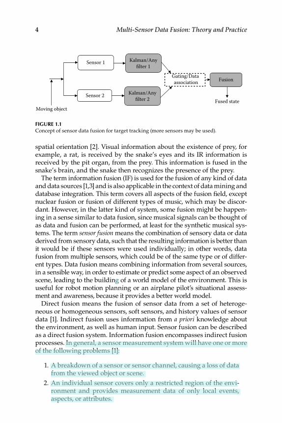
Animals recognize their changing environment by processing and evaluation of signals, such as data and some crude information, from mul-tiple directions and multiple sensors—sight, sound, touch, smell, and taste [1]. Nature, through the process of natural selection in very long cycles, has evolved a way to integrate the information from multiple sources and sensing organs to form a reliable recognition of an object, entity, scene, or phenomenon. Even in the case of signal or data loss from a sensor, certain systems are able to compensate for or tolerate the lack of information and continue to function at a lower, degraded level. They can do this because they reuse the data obtained from other similar or dissimilar sensors or sens-ing organs. Humans combine the signals and data from the body senses—sight, sound, touch, smell, and taste—with sometimes vague knowledge of the environment to create and update a dynamic model of the world in which they live and function. It is often said that humans even use the sixth sense! Based on this integrated information within the human brain, an individual interacts with the surrounding environment and makes deci-sions about her or his immediate present and near future actions [1]. This ability to fuse multisensory data has evolved due to a process popularly known as natural selection, which occurs to a high degree in many animal species, including humans, and has been happening for millions of years. Charles Darwin, some 150 years ago, and a few others have played a prom-inent role in understanding evolution. The use and application of sensor data fusion concepts in technical areas has led to new disciplines that span and infl uence many fi elds of science, engineering, and technology and that have been researched for the last few decades. A broad idea of sensor data fusion is depicted for target tracking in Figure 1.1.

The art of ventriloquism involves a process of human multisensory integration and fusion [2]. The visual information comes from the dum-my’s lips, which are moved and operated by the ventriloquist, and the auditory information comes from the ventriloquist herself. Although her mouth is closed, she transmits the auditory signal. This dual information is fused by the viewer and he or she feels as if the dummy is speaking, which particularly amuses the children. If the angle between the dummy’s lips and the ventriloquist’s face is more than 30°, then the coordination is very weak [2]. A rattlesnake is responsive to both visual and infrared (IR) infor-mation being represented on the surface of the optic tectum in a similar

4 Multi-Sensor Data Fusion: Theory and Practice

spatial orientation [2]. Visual information about the existence of prey, for example, a rat, is received by the snake’s eyes and its IR information is received by the pit organ, from the prey. This information is fused in the snake’s brain, and the snake then recognizes the presence of the prey.

The term information fusion (IF) is used for the fusion of any kind of data and data sources [1,3] and is also applicable in the context of data mining and database integration. This term covers all aspects of the fusion fi eld, except nuclear fusion or fusion of different types of music, which may be discor-dant. However, in the latter kind of system, some fusion might be happen-ing in a sense similar to data fusion, since musical signals can be thought of as data and fusion can be performed, at least for the synthetic musical sys-tems. The term sensor fusion means the combination of sensory data or data derived from sensory data, such that the resulting information is better than it would be if these sensors were used individually; in other words, data fusion from multiple sensors, which could be of the same type or of differ-ent types. Data fusion means combining information from several sources, in a sensible way, in order to estimate or predict some aspect of an observed scene, leading to the building of a world model of the environment. This is useful for robot motion planning or an airplane pilot’s situational assess-ment and awareness, because it provides a better world model.

Direct fusion means the fusion of sensor data from a set of heteroge-neous or homogeneous sensors, soft sensors, and history values of sensor data [1]. Indirect fusion uses information from a priori knowledge about the environment, as well as human input. Sensor fusion can be described as a direct fusion system. Information fusion encompasses indirect fusion processes. In general, a sensor measurement system will have one or more of the following problems [1]:

1. A breakdown of a sensor or sensor channel, causing a loss of data from the viewed object or scene.

2. An individual sensor covers only a restricted region of the envi-ronment and provides measurement data of only local events, aspects, or attributes.

Moving object

Sensor 1

Sensor 2

Kalman/Anyfilter 1

Fusion

Kalman/Anyfilter 2

Gating/Data association

Fused state

FIGURE 1.1 Concept of sensor data fusion for target tracking (more sensors may be used).

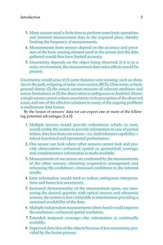
Introduction 5

3. Many sensors need a fi nite time to perform some basic operations and transmit measurement data to the required place, thereby limiting the frequency of measurements.

4. Measurements from sensors depend on the accuracy and preci-sion of the basic sensing element used in the sensor and the data gathered would thus have limited accuracy.

5. Uncertainty depends on the object being observed; if it is in a noisy environment, the measurement data noise effects would be present.

Uncertainty would arise if (1) some features were missing, such as obsta-cles in the path, eclipsing of radar cross section (RCS), Glint noise, or back-ground clutter; (2) the sensor cannot measure all relevant attributes and sensor limitations; or (3) the observation is ambiguous or doubtful. Hence, a single sensor cannot reduce uncertainty in its perception of the observed scene, and one of the effective solutions to many of the ongoing problems is multisensor data fusion.

By the fusion of sensors’ data we can expect one or more of the follow-ing potential advantages [1,4,5]:

1. Multiple sensors would provide redundancy which, in turn, would enable the system to provide information in case of partial failure, data loss from one sensor—i.e., fault tolerance capability—robust functional and operational performance.

2. One sensor can look where other sensors cannot look and pro-vide observations—enhanced spatial or geometrical coverage, and complementary information is made available.

3. Measurements of one sensor are confi rmed by the measurements of the other sensors, obtaining cooperative arrangement and enhancing the confi dence—increased confi dence in the inferred results.

4. Joint information would tend to reduce ambiguous interpreta-tions and hence less uncertainty.

5. Increased dimensionality of the measurement space, say mea-suring the desired quantity with optical sensors and ultrasonic sensors, the system is less vulnerable to interferences providing a sustained availability of the data.

6. Multiple independent measurements when fused would improve the resolution—enhanced spatial resolution.

7. Extended temporal coverage—the information is continually available.

8. Improved detection of the objects because of less uncertainty pro-vided by the fusion process.

6 Multi-Sensor Data Fusion: Theory and Practice

For a given data fusion system, one or more of the above benefi ts could occur. One can design and use the task-oriented multisensor data fusion (MSDF) system in order to obtain one or more of the above benefi ts.

When building an MSDF system, the following aspects pertaining to an actual application are of great importance: (1) use of optimal techniques and numerically stable and reliable algorithms for estimation, prediction, and image processing; (2) choice of data fusion architectures such as sensor nodes and the decision-making unit’s connectivity and data transmission aspects; (3) accuracy that can be realistically achieved by a data fusion pro-cess or system and conditions under which data fusion provides improved performance; and (4) keeping track of the data collection environment in a database management system. The main point is that one makes a syn-ergistic utilization of the data from multiple sensors to extract the greatest amount of information possible about the sensed object, scene, or envi-ronment. Humans use data from sight, sound, scent, touch, and a priori knowledge, then assess the world and events around them. This involves the conversion of these data (from images, sounds, smell, shapes, textures, etc.) into meaningful perceptions and features involving or leading to a large number of distinctly intelligent decision processes.

However, sensor or data fusion should not be considered as a universal method. Data fusion is a good idea, provided the data are of reasonably good quality. Just manipulating many bad data would not produce any great results—it might produce some results, but at a very high cost [1]. Many fused very poor quality sensors would not make up for a few good ones, and it may not be easy to fi x the errors in the initial processing of the data at a later stage, after the data have been processed and inferences are being drawn.

It is often said that the fusion of sensor data enhances accuracy, but of what? What is actually meant is that the overall accuracy of the prediction of the state of the system is increased. However, the accuracy of any sensor cannot increase beyond what is specifi ed by the manufacturer—that is the intrinsic accuracy. Ultimately, the idea is that the overall uncertainty level, after the fusion of data, is reduced, since information from various sen-sors is utilized in the fusion process. The point is that since uncertainty is reduced (and certainty is enhanced) the impression is that the accuracy has improved. It just makes sense to believe that the accuracy is increased, because the prediction is more certain than it would have been with only a single sensor. This is true even though the accuracy of the sensor cannot simply increase. Hence, the meaning of the term “increased accuracy” in the data fusion process, interpreted in the context of reduction of predic-tion uncertainty, should not create any fundamental confusion.

There are certain positive outlooks on the use and applications of MSDF [1]: (1) In reference [6] the authors present a proof that the use of additional sensors improves performance in the specifi c cases of majority vote and

Introduction 7

decision fusion; and (2) Dasarathy describes the benefi ts in increasing the number of inputs to the fusion process [7], and discusses what, where, why, when, and how the information fusion occurs in reference [3]. In the analysis limited to the augmentation of two-sensor systems by one addi-tional sensor, increasing the number of sensors may lead to a performance gain depending on the fusion algorithm employed.

There are several other applications where some benefi ts of MSDF have been realized; these can be found in the various references cited in this book. However, a slight skepticism on “perfect” or “optimal” fusion meth-ods is appropriate [1]. All DF systems may not be optimal, but some merit can be derived from these systems, which can be conditionally optimal or pareto-optimal. This should not prevent sensor data fusion activity, and should give impetus to data fusion activities to search for better and better data fusion solutions and systems with enhanced performance.

Fusion processes are often categorized in three levels of modes: low-, intermediate-, and high-level fusion, as follows:

1. Low-level fusion or raw-data fusion combines several sources of essentially the same type of raw preprocessed (RPP) data to pro-duce a new raw data set that is expected to be more informative and useful than the inputs. Of course, the data should be available in the required engineering units, and could even be RPP data. This can be expanded to include the fusion of estimated states of a system or object by using data from several, often dissimilar, sen-sors and is called state vector fusion. The entire process is called kinematic data fusion, which can include kinematic states as well as dynamic states. This is dealt with in Part I, along with some fundamental concepts of data fusion.

2. Intermediate-level, mid-level fusion, or feature-level fusion com-bines various features such as edges, lines, corners, textures, or positions into a feature map. This map is used for segmentation of images, detection of objects, etc. This process of fusion is called pixel-, feature-, or image-level fusion and is dealt with in Part III.

3. High-level fusion, or decision fusion, combines decisions from several experts. Methods of decision fusion are voting, fuzzy logic, and statistical methods. Some aspects, mainly fuzzy logic-based decision fusion, are dealt with in Part II.

In the following systems and applications, data fusion aspects can be incorporated, or data fusion can be utilized [2,8,9]:

1. Modular robotics: Such a system is constructed from a small number of standard units, with each module having its own

8 Multi-Sensor Data Fusion: Theory and Practice

hardware/software (HW/SW), driven and steered or controlled units, sensors, data communication links, power units, path- planning algorithms, obstacle avoidance provisions, sensor fusion, and control systems. There is no central processor on the vehicle. The vehicle employs multiple sensors to measure its body posi-tion, orientation, wheel position and velocities, obstacle locations, and changes in the terrain. The sensor data from the module are fused in a decentralized manner and used to generate local con-trol for each module. Such a modular system reduces cost and has fl exibility, increased system reliability, scalability and good survivability (and modularity).

2. The NASA Mars Pathfi nder Mission’s Sojourner Rover (1997): The autonomous operations are: terrain navigation, rock inspections, terrain mapping, and response to contingencies. It has fi ve laser stripe projectors and two charge-coupled device (CCD) cameras to detect and avoid rocks. It also has bumpers, articulation sensors, and accelerometers. It is an example of a multisensor or multi-actuator system. The fusion algorithms in the Rover are based on the state-space methods (extended Kalman fi lter [EKF] is used) and are centralized.

3. The Russian Mir Space Station and the Columbia Space Shuttle could use decentralized data fusion and control strategies.

4. A brief summary of data fusion applications in manufacturing and related processes is given in [9]:

a. Online prediction of surface fi nish and tool wear using a neu-ral network-based sensor fusion scheme to estimate, predict, and control the online surface fi nish.

b. A tool failure detection system using multisensor: A normal-ized mean cutting force derived from a tool dynamometer, maximum acceleration (obtained from an accelerometer), and an amplitude of displacement acquired from a gap sensor are fused to successfully detect impending tool breakage online.

c. Nondestructive testing (NDT) data fusion at pixel level: The fusion of data obtained from NDT of a carbon fi ber reinforced composite (CFC) material inspected using eddy current and infrared (IR) thermograph.

d. Data from three different types of sensors—acoustic emission sensor, vibration sensor, and motor current sensor—are com-bined to determine the tool wear. The wear data is categorized into four classes—no wear, little wear, medium wear, and high wear—and are defi ned in terms of fuzzy membership func-tions. Four different classifi cation tools—nearest neighbor,

Introduction 9

two types of artifi cial neural networks (ANN), and a fuzzy inference system (FIS)—are used to classify the incoming ware descriptive data from the different sensors. Then the decisions from these classifi ers are combined to derive the fi nal decision.

e. Nondestructive fl aw detection in concrete structures: The data from ultrasonic and impact echo tests are combined using Dempster–Shafer evidential reasoning models to accomplish decision-level identity fusion.

f. NDT: The information from heterogeneous data sources such as x-ray, ultrasonic, and eddy current is exploited in a synergy among complementary information.

Other possible applications of data fusion include [9]: (1) human identity verifi cation, (2) gas turbine power plants, (3) wind-tunnel fl ow measure-ments, and (4) mine detection. A survey of many systems that use data fusion aspects in military applications, as well as other nontraditional MSDF applications, is presented in [4].

Chapters 2 to 4 cover some important data fusion process models and propose a small modifi cation in one data fusion process model. They also cover estimation fusion models and rules, data fusion methods, and strat-egies and algorithms for kinematic-level data fusion (for tracking of mov-ing objects), and will present some performance studies.

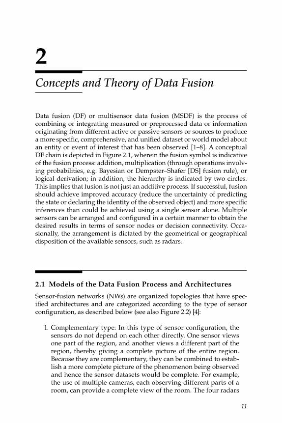
11

2 Concepts and Theory of Data Fusion

Data fusion (DF) or multisensor data fusion (MSDF) is the process of combining or integrating measured or preprocessed data or information originating from different active or passive sensors or sources to produce a more specifi c, comprehensive, and unifi ed dataset or world model about an entity or event of interest that has been observed [1–8]. A conceptual DF chain is depicted in Figure 2.1, wherein the fusion symbol is indicative of the fusion process: addition, multiplication (through operations involv-ing probabilities, e.g. Bayesian or Dempster–Shafer [DS] fusion rule), or logical derivation; in addition, the hierarchy is indicated by two circles. This implies that fusion is not just an additive process. If successful, fusion should achieve improved accuracy (reduce the uncertainty of predicting the state or declaring the identity of the observed object) and more specifi c inferences than could be achieved using a single sensor alone. Multiple sensors can be arranged and confi gured in a certain manner to obtain the desired results in terms of sensor nodes or decision connectivity. Occa-sionally, the arrangement is dictated by the geometrical or geographical disposition of the available sensors, such as radars.

2.1 Models of the Data Fusion Process and Architectures

Sensor-fusion networks (NWs) are organized topologies that have spec-ifi ed architectures and are categorized according to the type of sensor confi guration, as described below (see also Figure 2.2) [4]:

1. Complementary type: In this type of sensor confi guration, the sensors do not depend on each other directly. One sensor views one part of the region, and another views a different part of the region, thereby giving a complete picture of the entire region. Because they are complementary, they can be combined to estab-lish a more complete picture of the phenomenon being observed and hence the sensor datasets would be complete. For example, the use of multiple cameras, each observing different parts of a room, can provide a complete view of the room. The four radars

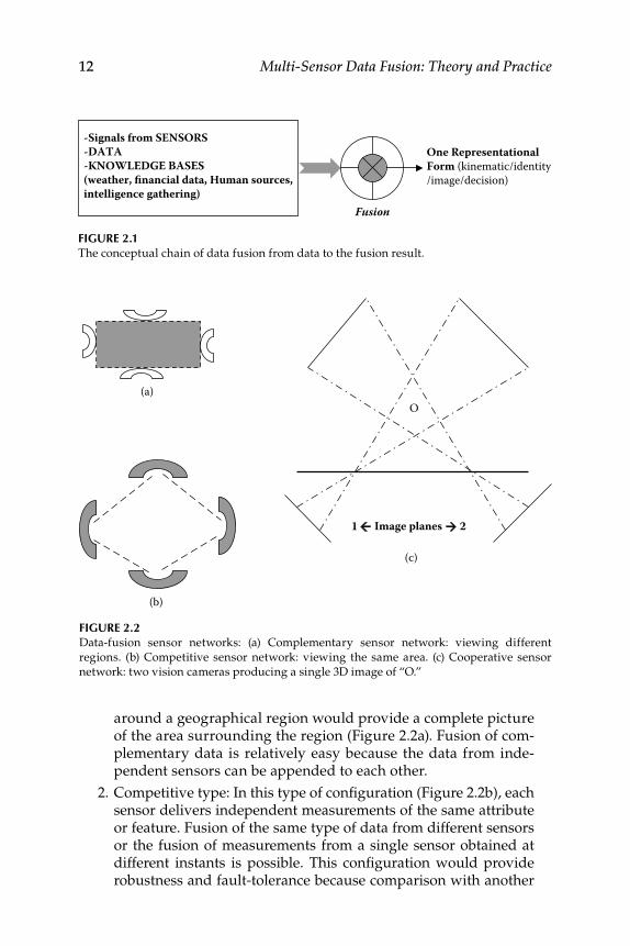
12 Multi-Sensor Data Fusion: Theory and Practice

around a geographical region would provide a complete picture of the area surrounding the region (Figure 2.2a). Fusion of com-plementary data is relatively easy because the data from inde-pendent sensors can be appended to each other.

2. Competitive type: In this type of confi guration (Figure 2.2b), each sensor delivers independent measurements of the same attribute or feature. Fusion of the same type of data from different sensors or the fusion of measurements from a single sensor obtained at different instants is possible. This confi guration would provide robustness and fault-tolerance because comparison with another

FIGURE 2.2 Data-fusion sensor networks: (a) Complementary sensor network: viewing different

regions. (b) Competitive sensor network: viewing the same area. (c) Cooperative sensor

network: two vision cameras producing a single 3D image of “O.”

(c)

(a)

(b)

O

1 Image planes 2

FIGURE 2.1 The conceptual chain of data fusion from data to the fusion result.

-Signals from SENSORS-DATA-KNOWLEDGE BASES(weather, financial data, Human sources,intelligence gathering)

One RepresentationalForm (kinematic/identity/image/decision)

Fusion

Concepts and Theory of Data Fusion 13

competitive sensor can be used to detect faults. Such robust systems can provide a degraded level of service in the presence of faults; moreover, the competing sensors in this system do not necessarily have to be identical.

3. Cooperative type: In this type of confi guration, data provided by two independent sensors are used to derive information that would not be available from a single sensor (see Figure 2.2c), as in a ste-reoscopic vision system. By combining the two-dimensional (2D) images from two cameras located at slightly different angles of inci-dence (viewed from two image planes), a three- dimensional (3D) image of the observed scene, marked “O,” is determined. Coopera-tive sensor fusion is diffi cult to design, and the resulting data will be sensitive to the inaccuracies in all the individual sensors.

In terms of usage, the three categories of sensor confi gurations are not mutually exclusive, because more than one of the three types of confi g-urations can be used in most cases. In a hybrid confi guration, multiple cameras that monitor a specifi c area can be used. In certain regions moni-tored by two or more cameras, the sensor confi guration could be either competitive or cooperative.

2.1.1 Data Fusion Models

MSDF is a system-theoretic process (a synergy of sensing, signal and data processing, estimation, control, and decision making) that is very involved, and hence an overall model that interconnects the various aspects and tasks of the DF activities is very much needed. This would also lend a systems approach to the DF process. We discuss several such models here.

2.1.1.1 Joint Directors of Laboratories Model

One very popular model, originating from the US Joint Directors of Lab- oratories (JDL), Department of Defense, is the JDL fusion model (DoD, USA, 1985/1992) [1,4]. The JDL model has fi ve levels of data processing and a database. These levels are interconnected by a common bus and need not be processed in a sequential order; nevertheless, they can be executed concurrently. There are three main levels—levels 1, 2, and 3, as shown in Figure 2.3 [1,4]. There are many sublevels and auxiliary levels for processing data, combining the available information, and evaluat-ing the performance of the DF system. Several such aspects are briefl y reviewed here. Although the terms used here have been borrowed from defense applications, similar terms are quite appropriate for other non- defense civilian DF applications. For such civilian applications, some

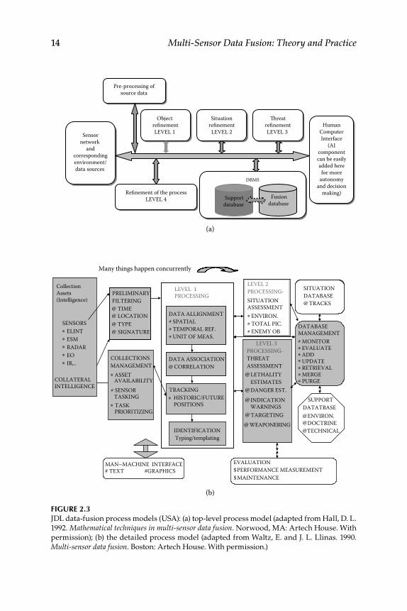
14 Multi-Sensor Data Fusion: Theory and Practice

FIGURE 2.3 JDL data-fusion process models (USA): (a) top-level process model (adapted from Hall, D. L.

1992. Mathematical techniques in multi-sensor data fusion. Norwood, MA: Artech House. With

permission); (b) the detailed process model (adapted from Waltz, E. and J. L. Llinas. 1990.

Multi-sensor data fusion. Boston: Artech House. With permission.)

(a)

(b)

PROCESSING-THREATASSESSMENT

Many things happen concurrently

LEVEL 2PROCESSING-SITUATIONASSESSMENT

LEVEL 3

SITUATIONDATABASE TRACKS

DATABASEMANAGEMENT

MAN–MACHINE INTERFACE# TEXT #GRAPHICS

$MAINTENANCE

EVALUATION$PERFORMANCE MEASUREMENT

CollectionAssets(Intelligence)

SENSORS ELINT ESM RADAR EO IR,..

COLLATERALINTELLIGENCE

PRELIMINARYFILTERING TIME LOCATION TYPE SIGNATURE

LEVEL 1PROCESSING

DATA ALLIGNMENT SPATIAL TEMPORAL REF. UNIT OF MEAS.

DATA ASSOCIATION CORRELATION

TRACKING HISTORIC/FUTURE POSITIONS

IDENTIFICATIONTyping/templating

Pre-processing ofsource data

Sensornetwork

andcorrespondingenvironment/data sources

Object refinementLEVEL 1

SituationrefinementLEVEL 2

ThreatrefinementLEVEL 3

Refinement of the processLEVEL 4

DBMS

Supportdatabase

Fusiondatabase

HumanComputerInterface

(AIcomponentcan be easilyadded herefor more

autonomyand decision

making)

@@@@*

****

*

*ENVIRON.*TOTAL PIC.*

MONITOREVALUATEADDUPDATERETRIEVALMERGEPURGE

*******

ENEMY OB***

**

*

COLLECTIONSMANAGEMENT

TASK

ASSET AVAILABILITY

SENSOR TASKING

PRIORITIZING

@

@

SUPPORTDATATBASE

ENVIRON.DOCTRINETECHNICAL

@@@

TARGETING@

WEAPONERING@

@ INDICATIONWARNINGS

@ LETHALITYESTIMATES

@ DANGER EST.

Concepts and Theory of Data Fusion 15

parts of the JDL model would be more appropriate, and interested users can determine the appropriate terms.

The JDL fusion-process model is a functionality-oriented DF model and is intended to be very general and useful across multiple applica-tion areas—from a sensor NW to the human-computer interface (HCI), with sub-buses having up to four levels of signal-fusion processing and performance evaluation. The output from the DF process in the model—the identifi cation and characterization of the individual entities or objects—is supposed to be minimally ambiguous [1,4]. It is also expected to facili-tate a higher-level interpretation of certain entities within the context of the intended application environment. The JDL-data fusion process (DFP) model is a conceptual model that identifi es the processes, functions, cat-egories of techniques, and specifi c techniques applicable for DF. DFP is defi ned and conceptualized by sources of information, human-computer interaction, preprocessing at the source, DF levels, and fi nally, the data-management system, including performance evaluation. The JDL model is an information-centered, abstract model, with specifi c characteristics as explained below [1,2,4].

Information from a variety of data sources, such as sensors, a priori infor-mation, databases, human input (called humint, for human intelligence), and electronic intelligence, is normally required and collected for DF. This could, in an overall sense, be called intelligence- collection assets, regardless of whether a particular sensor is intelligent or not. The idea is that some intelligence could have been used somewhere in the sensor system or NW. The sensor system could be called intelligent if it is sup-ported by mechanisms of artifi cial intelligence (AI), which utilize artifi -cial neural networks (ANNs) for learning, fuzzy logic (rule-based fuzzy approximate reasoning for logical decision making), and/or evolutionary algorithms for detection, acquisition, or preprocessing of measurements. The sources of information include [1,4] the following: (1) local sensors associated with the DF system, (2) distributed sensors linked electrically or through radio waves to a fusion system, and (3) reference information, geographical information, and so on. The collected data are preprocessed, and a preliminary fi ltering is attempted. The time and location and the type and signatures of the collected data are defi ned or determined at this level, often called level 0 (this is not explicitly indicated in Figure 2.3, but implied as a part of the second column). The data can be grouped and classifi ed, and some signatures can be added or integrated along with the type of the data. Priorities for the further processing of certain data can be assigned, and then level-1 processing can begin, as shown in Figure 2.3.

Object refi nement (level 1): At this level, several tasks are carried out, including data alignment (transformation of data into a consistent ref-erence frame and units), association (using correlation methods; bet-ter known as data association), tracking actual and future positions of

16 Multi-Sensor Data Fusion: Theory and Practice

objects, and identifi cation using classifi cation methods. This level con-sists of numerical procedures, such as estimation, target tracking, and pattern recognition. Object refi nement aids in object assessments by combining the location, parametric, and identity information to achieve refi ned representations of individual objects (such as emitters, platforms, and weapons) regarding their type, identity, position, velocity, accelera-tion, and so on. Level 1 performs the following four functions: (1) trans-forms data into a consistent set of units and coordinates; (2) refi nes and extends to a future time the estimates of an object’s position, kinematics, dynamics or attributes; (3) assigns data to the objects to allow the applica-tion of statistical estimation techniques; and (4) refi nes the estimation of an object’s identity or classifi cation. Level-1 fusion can be categorically divided into two parts: (1) kinematic fusion, which involves fusion of local information to determine the position, velocity, and acceleration of mov-ing objects, such as missile, aircraft, ships, people, and ground vehicles; and (2) identity fusion, which involves fusion of parametric data to deter-mine the identity of an observed object, e.g., deciding whether a moving object is a missile or an aircraft. Identity estimation can be augmented by rule-based expert systems, wherein various types of factual or procedural information can be exploited to aid the identity estimation.

Situation refi nement (level 2): In this level, an attempt is made to fi nd a contextual description of the relationship between the objects and observed events. After processing the data at level 1, the situation is ascer-tained and further analysis is carried out to refi ne the situation, if needed. The main goal is to obtain a total picture of the enemy’s objective for pur-poses such as defense application. This is a very complex process.

Threat refi nement (level 3): On the basis of the a priori knowledge and predictions about the future situation, inferences about vulnerabilities and opportunities for operation are constructed. During threat assess-ment, several aspects are considered, such as (1) estimation of danger, (2) indication of warning, and (3) targeting. The ultimate aim is to obtain a refi ned assessment of the threat (and its perception), on which important decisions and actions can be based.

Process refi nement, often added as level 4, is a metaprocess that moni-tors the system performance, e.g., real-time constraints, and reallocates sensors and sources to achieve particular goals or mission objectives. At this level, we are not concerned with the data (processing). However, sen-sor management is an appropriate aspect to study and employ at this level for optimal use of sensor suites.

Some DF theorists and practitioners also include the cognitive-refi nement level [4] as level 5, which is between level 3 and the HCI, thereby introducing the concept of AI at this stage in a limited manner.

The JDL model is supported by a database-management system, which monitors, evaluates, adds, updates, and provides information for the fusion

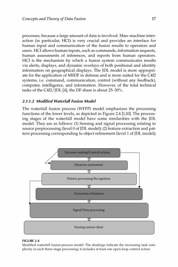
Concepts and Theory of Data Fusion 17

processes, because a large amount of data is involved. Man–machine inter-action (in particular, HCI) is very crucial and provides an interface for human input and communication of the fusion results to operators and users. HCI allows human inputs, such as commands, information requests, human assessments of inferences, and reports from human operators. HCI is the mechanism by which a fusion system communicates results via alerts, displays, and dynamic overlays of both positional and identity information on geographical displays. The JDL model is more appropri-ate for the application of MSDF in defense and is more suited for the C4I2 systems, i.e. command, communication, control (without any feedback), computer, intelligence, and information. However, of the total technical tasks of the C4I2/JDL [4], the DF share is about 25–30%.

2.1.1.2 Modifi ed Waterfall Fusion Model

The waterfall fusion process (WFFP) model emphasizes the processing functions of the lower levels, as depicted in Figure 2.4 [1,10]. The process-ing stages of the waterfall model have some similarities with the JDL model. They are as follows: (1) Sensing and signal processing relating to source preprocessing (level 0 of JDL model); (2) feature extraction and pat-tern processing corresponding to object refi nement (level 1 of JDL model);

Sensing (sensor data)

Signal/Data processing

Extraction of features

Pattern processing/Recognition

Situation assessment

Decision making/Control actions

FIGURE 2.4 Modifi ed waterfall fusion-process model: The shadings indicate the increasing task com-

plexity in each three-stage processing; it includes at least one open-loop control action.

18 Multi-Sensor Data Fusion: Theory and Practice

(3) situation assessment (SA) relating to situation refi nement (level 2 of JDL model); and (4) decision making relating to threat refi nement (level 3 of JDL model). The WFFP model is similar in some aspects to the JDL model; however, the WFFP model is very easy to apply. There is no feed-back of data fl ow in the WFFP model because this is an acyclic model. In Figure 2.4, a modifi ed WFFP model is proposed and presented, where (1) the increasing complexity of the subtask is indicated by darker shades within the fi rst (from sensing to extraction of features) and second (from pattern processing to decision making and control actions) stages of the three-stage process; and (2) there are some feedback loops. The model rep-resented in Figure 2.4 is a modifi ed version of the original model [1,10] and can include at least one open-loop control action or some feedback-loop control actions. Thus, the proposed modifi ed WFFP model is an action-oriented model. It has been modifi ed using local feedback loops, as fol-lows (Figure 2.4): (1) From the decision making and control actions to the situation-assessment block, to refl ect the situation refi nement and its use as new control action; (2) from pattern processing to signal processing, to refl ect the enhanced pattern recognition and its use in refi ning the SA; and (3) from the decision making and control actions to the feature- extraction block, to refl ect the improved decision making process and new control action based on the enhanced feature extraction. Thus, the modi-fi ed WFFP model is more than an abstract model; it is action-oriented, when compared with the JDL or the conventional WFFP models.

2.1.1.3 Intelligence Cycle–Based Model

Because the DF process has some inherent cyclic processing behavior that is not captured in the JDL model, the intelligence cycle–based (IC) model tries to capture these cyclic characteristics [1,11], comprised of the following fi ve stages:

1. In the planning and direction stage, the intelligence requirements are determined.

2. In the collection stage, the appropriate information is gathered.

3. In the collation stage, the collected information is streamlined.

4. In the evaluation stage, the available information is used and the actual fusion is carried out.

5. In the dissemination stage, the fused intelligence and inferences are distributed.

This model is a macrolevel data-processing DF model and looks more like a top-level model than the WFFP model. The sublevel actions and pro-cessing tasks are not defi ned or indicated in the IC model, although these

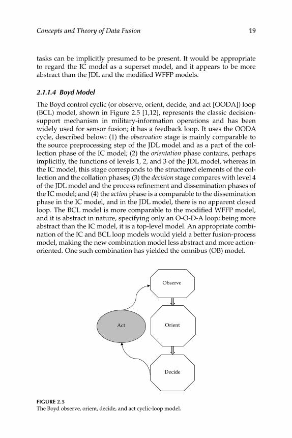
Concepts and Theory of Data Fusion 19

tasks can be implicitly presumed to be present. It would be appropriate to regard the IC model as a superset model, and it appears to be more abstract than the JDL and the modifi ed WFFP models.

2.1.1.4 Boyd Model

The Boyd control cyclic (or observe, orient, decide, and act [OODA]) loop (BCL) model, shown in Figure 2.5 [1,12], represents the classic decision- support mechanism in military-information operations and has been widely used for sensor fusion; it has a feedback loop. It uses the OODA cycle, described below: (1) the observation stage is mainly comparable to the source preprocessing step of the JDL model and as a part of the col-lection phase of the IC model; (2) the orientation phase contains, perhaps implicitly, the functions of levels 1, 2, and 3 of the JDL model, whereas in the IC model, this stage corresponds to the structured elements of the col-lection and the collation phases; (3) the decision stage compares with level 4 of the JDL model and the process refi nement and dissemination phases of the IC model; and (4) the action phase is a comparable to the dissemination phase in the IC model, and in the JDL model, there is no apparent closed loop. The BCL model is more comparable to the modifi ed WFFP model, and it is abstract in nature, specifying only an O-O-D-A loop; being more abstract than the IC model, it is a top-level model. An appropriate combi-nation of the IC and BCL loop models would yield a better fusion-process model, making the new combination model less abstract and more action-oriented. One such combination has yielded the omnibus (OB) model.

FIGURE 2.5 The Boyd observe, orient, decide, and act cyclic-loop model.

Observe

Orient

Decide

Act

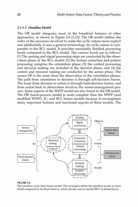
20 Multi-Sensor Data Fusion: Theory and Practice

2.1.1.5 Omnibus Model

The OB model integrates most of the benefi cial features of other approaches, as shown in Figure 2.6 [1,13]. The OB model defi nes the order of the processes involved to make the cyclic nature more explicit and additionally, it uses a general terminology. Its cyclic nature is com-parable to the BCL model. It provides reasonably detailed processing levels compared to the BCL model. The various levels are as follows: (1) The sensing and signal processing steps are conducted by the obser-vation phase of the BCL model; (2) the feature extraction and pattern processing comprise the orientation phase; (3) the context processing and decision making are included in the decision phase; and (4) the control and resource tasking are conducted by the action phase. The sensor DF is the route from the observation to the orientation phases. The path from orientation to decision is through soft-decision fusion. The route from decision to action is through hard-decision fusion, and from action back to observation involves the sensor- management pro-cess. Some aspects of the WFFP model are also found in the OB model. The OB fusion-process model is more complete than the WFFP (and modifi ed WFFP), IC, and BCL fusion models because it encompasses many important features and functional aspects of these models. The

Observe

Orient

Decide

Act

Control

Resourcetasking

DecisionmakingContext

processing

Extraction of features

Pattern processing

Signal processing

Sensing

Sensor datafusion

Soft decisionfusion Hard decision

fusion

Sensormanagement

FIGURE 2.6 The omnibus cyclic data-fusion model: The rectangles defi ne the omnibus model in more

detail compared to the Boyd observe, orient, decide, and act model (BCL in dotted lines).

Concepts and Theory of Data Fusion 21

OB model is simple and easy to apply and follow for many non- defense DF applications. In addition, the OB model is more generalized than the previous three models and has a cyclic and closed-loop action ele-ment, making it more attractive than the JDL fusion model. Thus, the OB model can be regarded as the standard fusion-process model for non-defense DF processing and applications.

2.1.2 Fusion Architectures

The MSDF process, as described above, involves integration of sensors, data preprocessing, estimation, and a further higher level of processing and decision making. It demands a defi nite arrangement of sensors and sensor-data acquisition systems and signal-processing aspects, which are, in turn, dictated by the fusion architectures. Mainly, there are three types of architecture, as discussed in Sections 2.1.2.1 to 2.1.2.3 [4,8].

2.1.2.1 Centralized Fusion

Centralized fusion architecture, as shown in Figure 2.7a [4], used mainly for similar sensors, involves time-synchronization and bias correction of sensor data, transformation of the sensor data from sensor-based units and coordinates into convenient coordinates and units for central process-ing, e.g., polar to earth–centered, earth-fi xed coordinates, gating and asso-ciation in case of multiple targets, and measurement fusion. Decisions are based on the maximum possible information gathered from the system of sensors, also called measurement fusion. Thus, centralized fusion is a conventional estimation problem with distributed data.

2.1.2.2 Distributed Fusion

Distributed fusion (Figure 2.7b) [4,8] is mainly used for dissimilar sensors (sensors with different observation frames) i.e. infrared and radar; how-ever, it can still be used for similar types of sensors. In this architecture, observation data from each sensor is processed by an individual Kalman fi lter (KF), extended KF, or square-root information fi lter (SRIF) at each node. The local track, consisting of the estimated state vector and cova-riance matrix from each fi lter, is used as input to the state-vector fusion process, and the output is the fused state vector and its (fused) covari-ance matrix. The information is processed locally at each node; there is no central fusion here. This architecture is useful for large fl exible and smart structures, monitoring of aircraft or spacecraft health, huge automated plants, large sensor NWs, and chemical industries. This is also referred to as estimation fusion (EF) in target-tracking applications.

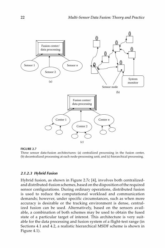
22 Multi-Sensor Data Fusion: Theory and Practice

2.1.2.3 Hybrid Fusion

Hybrid fusion, as shown in Figure 2.7c [4], involves both centralized- and distributed-fusion schemes, based on the disposition of the required sensor configurations. During ordinary operations, distributed fusion is used to reduce the computational workload and communication demands; however, under specific circumstances, such as when more accuracy is desirable or the tracking environment is dense, central-ized fusion can be used. Alternatively, based on the sensors avail-able, a combination of both schemes may be used to obtain the fused state of a particular target of interest. This architecture is very suit-able for the data processing and fusion system of a flight-test range (in Sections 4.1 and 4.2, a realistic hierarchical MSDF scheme is shown in Figure 4.1).

FIGURE 2.7 Three sensor data-fusion architectures: (a) centralized processing in the fusion center,

(b) decentralized processing at each node-processing unit, and (c) hierarchical processing.

(a)

(b)

(c)

Fusion center/data processing

Sensor 1

Sensor 2

Sensor n

Systemmonitor

Sensor node

Fusion center/data processing

Center 1

Center 2

Center n

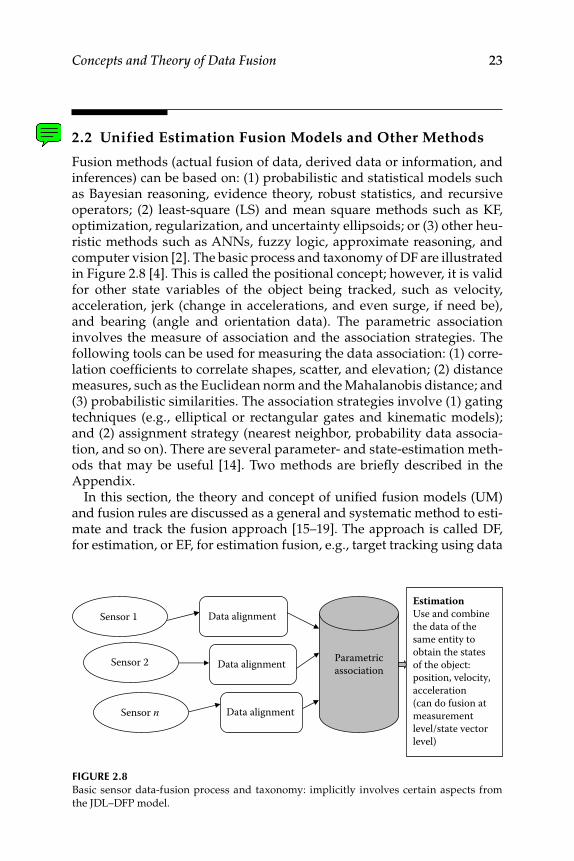
Concepts and Theory of Data Fusion 23

2.2 Unified Estimation Fusion Models and Other Methods

Fusion methods (actual fusion of data, derived data or information, and inferences) can be based on: (1) probabilistic and statistical models such as Bayesian reasoning, evidence theory, robust statistics, and recursive operators; (2) least-square (LS) and mean square methods such as KF, optimization, regularization, and uncertainty ellipsoids; or (3) other heu-ristic methods such as ANNs, fuzzy logic, approximate reasoning, and computer vision [2]. The basic process and taxonomy of DF are illustrated in Figure 2.8 [4]. This is called the positional concept; however, it is valid for other state variables of the object being tracked, such as velocity, acceleration, jerk (change in accelerations, and even surge, if need be), and bearing (angle and orientation data). The parametric association involves the measure of association and the association strategies. The following tools can be used for measuring the data association: (1) corre-lation coeffi cients to correlate shapes, scatter, and elevation; (2) distance measures, such as the Euclidean norm and the Mahalanobis distance; and (3) probabilistic similarities. The association strategies involve (1) gating techniques (e.g., elliptical or rectangular gates and kinematic models); and (2) assignment strategy (nearest neighbor, probability data associa-tion, and so on). There are several parameter- and state-estimation meth-ods that may be useful [14]. Two methods are briefl y described in the Appendix.

In this section, the theory and concept of unifi ed fusion models (UM) and fusion rules are discussed as a general and systematic method to esti-mate and track the fusion approach [15–19]. The approach is called DF, for estimation, or EF, for estimation fusion, e.g., target tracking using data

FIGURE 2.8 Basic sensor data-fusion process and taxonomy: implicitly involves certain aspects from

the JDL–DFP model.

Sensor 1

Sensor 2

Sensor n

Data alignment

Data alignment

Data alignment

Parametricassociation

EstimationUse and combinethe data of thesame entity toobtain the statesof the object:position, velocity,acceleration(can do fusion atmeasurementlevel/state vectorlevel)

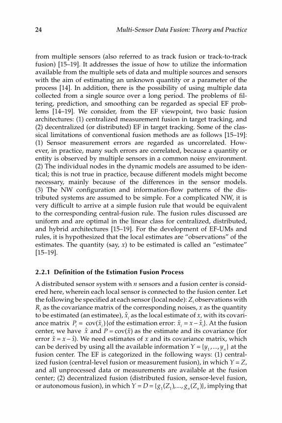
24 Multi-Sensor Data Fusion: Theory and Practice

from multiple sensors (also referred to as track fusion or track-to-track fusion) [15–19]. It addresses the issue of how to utilize the information available from the multiple sets of data and multiple sources and sensors with the aim of estimating an unknown quantity or a parameter of the process [14]. In addition, there is the possibility of using multiple data collected from a single source over a long period. The problems of fi l-tering, prediction, and smoothing can be regarded as special EF prob-lems [14–19]. We consider, from the EF viewpoint, two basic fusion architectures: (1) centralized measurement fusion in target tracking, and (2) decentralized (or distributed) EF in target tracking. Some of the clas-sical limitations of conventional fusion methods are as follows [15–19]: (1) Sensor measurement errors are regarded as uncorrelated. How-ever, in practice, many such errors are correlated, because a quantity or entity is observed by multiple sensors in a common noisy environment. (2) The individual nodes in the dynamic models are assumed to be iden-tical; this is not true in practice, because different models might become necessary, mainly because of the differences in the sensor models. (3) The NW confi guration and information-fl ow patterns of the dis-tributed systems are assumed to be simple. For a complicated NW, it is very diffi cult to arrive at a simple fusion rule that would be equivalent to the corresponding central-fusion rule. The fusion rules discussed are uniform and are optimal in the linear class for centralized, distributed, and hybrid architectures [15–19]. For the development of EF-UMs and rules, it is hypothesized that the local estimates are “observations” of the estimates. The quantity (say, x ) to be estimated is called an “estimatee” [15–19].

2.2.1 Definition of the Estimation Fusion Process

A distributed sensor system with n sensors and a fusion center is consid-ered here, wherein each local sensor is connected to the fusion center. Let the following be specifi ed at each sensor (local node): Zi observations with Ri as the covariance matrix of the corresponding noises, x as the quantity to be estimated (an estimatee), xi as the local estimate of x, with its covari-ance matrix Pi = cov( %xi ) {of the estimation error: %xi = x − xi}. At the fusion center, we have x and P = cov( %x) as the estimate and its covariance (for error %x = x − x). We need estimates of x and its covariance matrix, which can be derived by using all the available information Y = {y

1, ..., yn } at the

fusion center. The EF is categorized in the following ways: (1) central-ized fusion (central-level fusion or measurement fusion), in which Y = Z , and all unprocessed data or measurements are available at the fusion center; (2) decentralized fusion (distributed fusion, sensor-level fusion, or autonomous fusion), in which Y = D = {g

1(Z

1), ..., gn(Zn )}, implying that

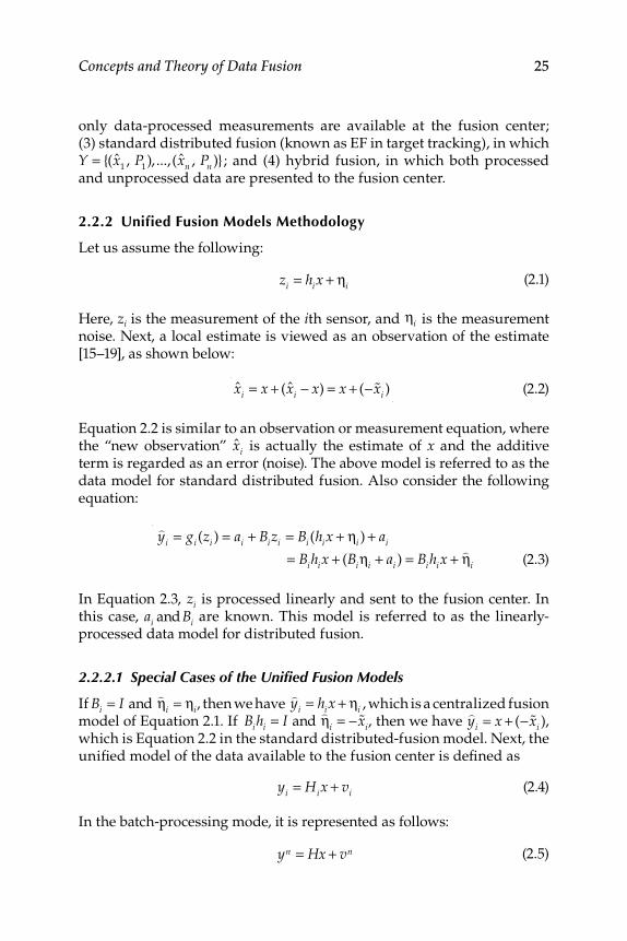
Concepts and Theory of Data Fusion 25

only data-processed measurements are available at the fusion center; (3) standard distributed fusion (known as EF in target tracking), in which Y = {(x

1, P

1), ..., (xn , Pn )}; and (4) hybrid fusion, in which both processed

and unprocessed data are presented to the fusion center.

2.2.2 Unified Fusion Models Methodology

Let us assume the following:

zi = hix + ηi (2.1)

Here, zi is the measurement of the i th sensor, and ηi is the measurement noise. Next, a local estimate is viewed as an observation of the estimate [15–19], as shown below:

xi = x + (xi − x) = x + (− %xi ) (2.2)

Equation 2.2 is similar to an observation or measurement equation, where the “new observation” xi is actually the estimate of x and the additive term is regarded as an error (noise). The above model is referred to as the data model for standard distributed fusion. Also consider the following equation:

)yi = gi (zi ) = ai + Bizi = Bi (hix + ηi ) + ai

= Bihix + (Biηi + ai ) = Bihix + )ηi (2.3)

In Equation 2.3, zi is processed linearly and sent to the fusion center. In this case, ai and Bi are known. This model is referred to as the linearly-processed data model for distributed fusion.

2.2.2.1 Special Cases of the Unifi ed Fusion Models

If Bi = I and)ηi = ηi, then we have

)yi = hix + ηi , which is a centralized fusion

model of Equation 2.1. If Bihi = I and)ηi = − %xi, then we have

)yi = x + (− %xi ),

which is Equation 2.2 in the standard distributed-fusion model. Next, the unifi ed model of the data available to the fusion center is defi ned as

yi = Hix + vi (2.4)

In the batch-processing mode, it is represented as follows:

yn = Hx + vn

(2.5)

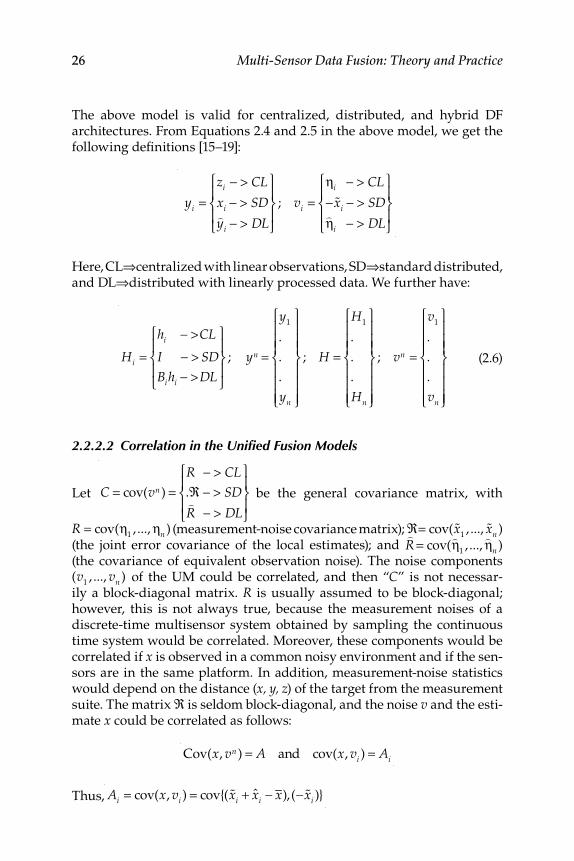
26 Multi-Sensor Data Fusion: Theory and Practice

The above model is valid for centralized, distributed, and hybrid DF architectures. From Equations 2.4 and 2.5 in the above model, we get the following defi nitions [15–19]:

yi =zi − > CL

xi − > SD)yi − > DL

⎧

⎨⎪

⎩⎪

⎫

⎬⎪

⎭⎪

; vi =ηi − > CL

− %xi − > SD)ηi − > DL

⎧

⎨⎪

⎩⎪

⎫

⎬⎪

⎭⎪

Here, CL⇒centralized with linear observations, SD⇒standard distributed, and DL⇒distributed with linearly processed data. We further have:

Hi =

hi − >CL

I − > SD

Bihi − > DL

⎧

⎨⎪

⎩⎪

⎫

⎬⎪

⎭⎪

; yn =

y1

.

.

.

yn

⎧

⎨

⎪⎪⎪

⎩

⎪⎪⎪

⎫

⎬

⎪⎪⎪

⎭

⎪⎪⎪

; H =

H1

.

.

.

Hn

⎧

⎨

⎪⎪⎪

⎩

⎪⎪⎪

⎫

⎬

⎪⎪⎪

⎭

⎪⎪⎪

; vn =

v1

.

.

.

vn

⎧

⎨

⎪⎪⎪

⎩

⎪⎪⎪

⎫

⎬

⎪⎪⎪

⎭

⎪⎪⎪

(2.6)

2.2.2.2 Correlation in the Unifi ed Fusion Models

Let C = cov(vn ) =R − > CL

.ℜ − > SD)R − > DL

⎧

⎨⎪

⎩⎪

⎫

⎬⎪

⎭⎪

be the general covariance matrix, with

R = cov(η1, ..., ηn ) (measurement-noise covariance matrix); ℜ= cov( %x

1, ..., %xn )

(the joint error covariance of the local estimates); and )R = cov(

)η1, ...,

)ηn ) (the covariance of equivalent observation noise). The noise components (v

1, ..., vn ) of the UM could be correlated, and then “ C ” is not necessar-

ily a block-diagonal matrix. R is usually assumed to be block-diagonal; however, this is not always true, because the measurement noises of a discrete-time multisensor system obtained by sampling the continuous time system would be correlated. Moreover, these components would be correlated if x is observed in a common noisy environment and if the sen-sors are in the same platform. In addition, measurement-noise statistics would depend on the distance ( x, y, z ) of the target from the measurement suite. The matrix ℜ is seldom block-diagonal, and the noise v and the esti-mate x could be correlated as follows:

Cov(x, vn ) = A and cov(x, vi ) = Ai

Thus, Ai = cov(x, vi ) = cov{( %xi + xi − x),(− %xi )}

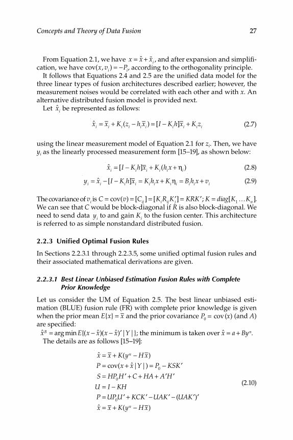
Concepts and Theory of Data Fusion 27

From Equation 2.1, we have x = x + %xi , and after expansion and simplifi -cation, we have cov(x, vi ) = −Pi, according to the orthogonality principle.

It follows that Equations 2.4 and 2.5 are the unifi ed data model for the three linear types of fusion architectures described earlier; however, the measurement noises would be correlated with each other and with x . An alternative distributed fusion model is provided next.

Let xi be represented as follows:

xi = xi + Ki (zi − hixi ) = [I − Kih]xi + Kizi

(2.7)

using the linear measurement model of Equation 2.1 for zi. Then, we have yi as the linearly processed measurement form [15–19], as shown below:

xi = [I − Kih]xi + Ki (hix + ηi )

(2.8)

yi = xi − [I − Kih]xi = Kihix + Kiηi = Bihix + vi

(2.9)

The covariance of vi is C = cov(v) = [Cij ] = [KiRij ′Kj ] = KR ′K ; K = diag[K

1KKn ].

We can see that C would be block-diagonal if R is also block-diagonal. We need to send data yi to and gain Ki to the fusion center. This architecture is referred to as simple nonstandard distributed fusion.

2.2.3 Unified Optimal Fusion Rules

In Sections 2.2.3.1 through 2.2.3.5, some unifi ed optimal fusion rules and their associated mathematical derivations are given.

2.2.3.1 Best Linear Unbiased Estimation Fusion Rules with Complete Prior Knowledge

Let us consider the UM of Equation 2.5. The best linear unbiased esti-mation (BLUE) fusion rule (FR) with complete prior knowledge is given when the prior mean E{x} = x and the prior covariance P

0= cov(x) (and A)

are specifi ed:

xB = arg min E{(x − x)(x − x ′) |Y|}; the minimum is taken over x = a + Byn. The details are as follows [15–19]:

x = x + K(yn − H x)

P = cov(x + x|Y|) = P0

− KS ′K

S = HP0 ′H + C + HA + ′A ′H

U = I − KH

P = UP0 ′U + KC ′K −UA ′K − (UA ′K ′)

x = x + K(yn − H x)

(2.10)

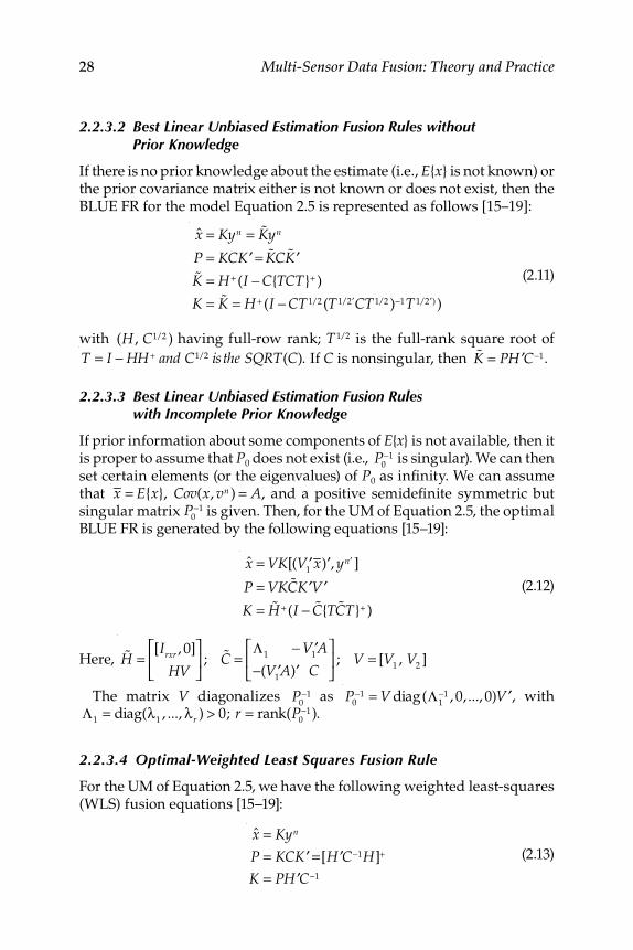
28 Multi-Sensor Data Fusion: Theory and Practice

2.2.3.2 Best Linear Unbiased Estimation Fusion Rules without Prior Knowledge

If there is no prior knowledge about the estimate (i.e., E { x } is not known) or the prior covariance matrix either is not known or does not exist, then the BLUE FR for the model Equation 2.5 is represented as follows [15–19]:

x = Kyn = %Kyn

P = KC ′K = %KC % ′K%K = H + (I − C{TCT}+ )

K = %K = H + (I − CT1/2 (T1/ ′2 CT1/2 )−1T1/ ′2 ) )

(2.11)

with (H , C1/2 ) having full-row rank; T1/2 is the full-rank square root of

T = I − HH + and C1/2 isthe SQRT(C). If C is nonsingular, then %K = P ′H C−1.

2.2.3.3 Best Linear Unbiased Estimation Fusion Rules with Incomplete Prior Knowledge

If prior information about some components of E { x } is not available, then it is proper to assume that P0 does not exist (i.e.,

P

0−1 is singular). We can then

set certain elements (or the eigenvalues) of P0 as infi nity. We can assume that x = E{x}, Cov(x, vn ) = A, and a positive semidefi nite symmetric but singular matrix P0

−1 is given. Then, for the UM of Equation 2.5, the optimal BLUE FR is generated by the following equations [15–19]:

x = VK[( ′V1

x ′) , y ′n ]

P = VK %C ′K ′V

K = %H + (I − %C{T %CT}+ )

(2.12)

Here,

%H =[Irxr , 0]

HV

⎡

⎣⎢

⎤

⎦⎥ ; %C =

Λ1

− ′V1A

−( ′V1A ′) C

⎡

⎣⎢

⎤

⎦⎥ ; V = [V

1, V

2]

The matrix V diagonalizes P

0−1 as P

0−1 = V diag(Λ

1−1 , 0, ..., 0) ′V , with

Λ1

= diag(λ1, ..., λr ) > 0; r = rank(P

0−1).

2.2.3.4 Optimal-Weighted Least Squares Fusion Rule

For the UM of Equation 2.5, we have the following weighted least-squares (WLS) fusion equations [15–19]:

x = Kyn

P = KC ′K =[ ′H C−1H]+

K = P ′H C−1

(2.13)

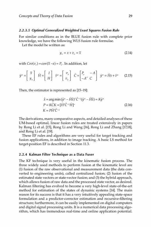
Concepts and Theory of Data Fusion 29

2.2.3.5 Optimal Generalized Weighted Least Squares Fusion Rule

For similar conditions as in the BLUE fusion rule with complete prior knowledge, we have the following WLS fusion rule formulae.

Let the model be written as:

yo = x + vo = x

(2.14)

with Cov(vo ) = cov(x −x) = Po . In addition, let

)yn =

x

yn

⎡

⎣⎢

⎤

⎦⎥

)H =

I

H

⎡

⎣⎢

⎤

⎦⎥

)vn =

vo

vn

⎡

⎣⎢

⎤

⎦⎥

)C =

Po − A

− ′A C

⎡

⎣⎢

⎤

⎦⎥

)yn =

)Hx + )

vn

(2.15)

Then, the estimator is represented as [15–19]:

x = arg min()yn −

)Hx ′)

)C−1(

)yn −

)Hx) = K

)yn

P = K)CK = [

)′H)C−1

)H]+

K = P)

′H)C−1

(2.16)

The derivations, many comparative aspects, and detailed analyses of these UM-based optimal, linear fusion rules are treated extensively in papers by Rong Li et al. [15], Rong Li and Wang [16], Rong Li and Zhang [17,18], and Rong Li et al. [19].

These EF rules and algorithms are very useful for target tracking and fusion applications, in addition to image tracking. A basic LS method for target-position EF is described in Section 11.3.

2.2.4 Kalman Filter Technique as a Data Fuser

The KF technique is very useful in the kinematic fusion process. The three widely used methods to perform fusion at the kinematic level are (1) fusion of the raw observational and measurement data (the data con-verted to engineering units), called centralized fusion; (2) fusion of the estimated state vectors or state-vector fusion; and (3) the hybrid approach, which allows fusion of raw data and the processed state vector, as desired. Kalman fi ltering has evolved to become a very high-level state-of-the-art method for estimation of the states of dynamic systems [14]. The main reason for its success is that it has a very intuitively appealing state-space formulation and a predictor-corrector estimation and recursive-fi ltering structure; furthermore, it can be easily implemented on digital computers and digital signal processing units. It is a numerical data processing algo-rithm, which has tremendous real-time and online application potential.

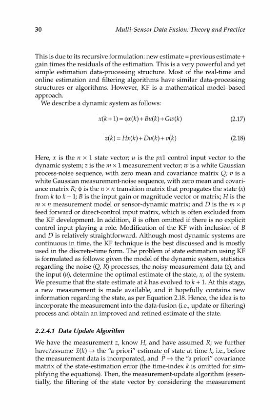
30 Multi-Sensor Data Fusion: Theory and Practice

This is due to its recursive formulation: new estimate = previous estimate + gain times the residuals of the estimation. This is a very powerful and yet simple estimation data-processing structure. Most of the real-time and online estimation and fi ltering algorithms have similar data-processing structures or algorithms. However, KF is a mathematical model–based approach.

We describe a dynamic system as follows:

x(k + 1) = φx(k) + Bu(k) + Gw(k)

(2.17)

z(k) = Hx(k) + Du(k) + v(k)

(2.18)

Here, x is the n × 1 state vector; u is the px 1 control input vector to the dynamic system; z is the m × 1 measurement vector; w is a white Gaussian process-noise sequence, with zero mean and covariance matrix Q; v is a white Gaussian measurement-noise sequence, with zero mean and covari-ance matrix R; φ is the n × n transition matrix that propagates the state ( x ) from k to k + 1; B is the input gain or magnitude vector or matrix; H is the m × n measurement model or sensor-dynamic matrix; and D is the m × p feed forward or direct-control input matrix, which is often excluded from the KF development. In addition, B is often omitted if there is no explicit control input playing a role. Modifi cation of the KF with inclusion of B and D is relatively straightforward. Although most dynamic systems are continuous in time, the KF technique is the best discussed and is mostly used in the discrete-time form. The problem of state estimation using KF is formulated as follows: given the model of the dynamic system, statistics regarding the noise ( Q , R ) processes, the noisy measurement data ( z ), and the input ( u ), determine the optimal estimate of the state, x , of the system. We presume that the state estimate at k has evolved to k + 1. At this stage, a new measurement is made available, and it hopefully contains new information regarding the state, as per Equation 2.18. Hence, the idea is to incorporate the measurement into the data-fusion (i.e., update or fi ltering) process and obtain an improved and refi ned estimate of the state.

2.2.4.1 Data Update Algorithm

We have the measurement z , know H, and have assumed R; we further

have/assume %x(k) → the “a priori” estimate of state at time k , i.e., before the measurement data is incorporated, and %P → the “a priori” covariance matrix of the state-estimation error (the time-index k is omitted for sim-plifying the equations). Then, the measurement-update algorithm (essen-tially, the fi ltering of the state vector by considering the measurement

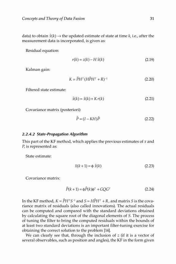
Concepts and Theory of Data Fusion 31

data) to obtain x(k) → the updated estimate of state at time k , i.e., after the measurement data is incorporated, is given as:

Residual equation:

r(k) = z(k) − H %x(k) (2.19)

Kalman gain:

K = %PHT (H %PHT + R)−1 (2.20)

Filtered state estimate:

x(k) = %x(k) + K r(k)

(2.21)

Covariance matrix (posteriori):

P = (I − KH) %P (2.22)

2.2.4.2 State-Propagation Algorithm

This part of the KF method, which applies the previous estimates of x and P, is represented as:

State estimate:

%x(k + 1) = φ x(k)

(2.23)

Covariance matrix:

%P(k + 1) = φP(k)φT + GQGT (2.24)

In the KF method, K = %PHTS−1 and S = H %PHT + R , and matrix S is the cova-riance matrix of residuals (also called innovations). The actual residuals can be computed and compared with the standard deviations obtained by calculating the square root of the diagonal elements of S . The process of tuning the fi lter to bring the computed residuals within the bounds of at least two standard deviations is an important fi lter-tuning exercise for obtaining the correct solution to the problem [14].

We can clearly see that, through the inclusion of z (if it is a vector of several observables, such as position and angles), the KF in the form given

32 Multi-Sensor Data Fusion: Theory and Practice

above is itself a measurement data–level fusion algorithm. It combines the measurements of these observables directly at the data level and pro-duces an optimal estimate of the state x . For each measurement type, one should choose appropriate H vectors or matrices and their corresponding R matrices. Therefore, the KF fundamentally accomplishes a DF task. The other fusion process, state-vector fusion, is illustrated in Section 3.1.1 (also, refer Exercise I.26).

2.2.5 Inference Methods

An inference (based on some initial observations) [2,4,20,21] is defi ned as an act of passing from one proposition, statement, or judgment considered or believed to be true to another, whose truth is believed to follow, by some logic, formulae, or process, from that of the former proposition or statement. Inference methods (IM) are used for decision making or fusion to arrive at a decision from the available knowledge. The decision con-cerning whether the road in front of a vehicle is blocked or free, given the measurements of multiple distance sensors, can be regarded as an infer-ence problem. The classical IM conducts tests on an assumed hypothesis to an alternative hypothesis, and it yields the probability of the actually observed data being present if the chosen hypothesis were true. The classical IM does not support the usage of a priori information about the probability of a proposed hypothesis, whereas the a priori probability is taken into account in the Bayesian inference method (BIM). The Bayesian theorem quantifi es the probability of hypothesis H , given that an event E has occurred. Using multiple hypotheses, the BIM can be used for solv-ing classifi cation problems; the Bayes’ rule will then produce a probabil-ity for each hypothesis. Due to certain limitations of the BIM, Dempster [20] generalized the Bayesian theory of subjective probability. Dempster’s rule of combination, which operates on belief or mass functions as Bayes’ rule does on probabilities, was more advanced. Shafer extended Demp-ster’s work and developed a mathematical theory of evidence [21], which can be applied for representation of incomplete knowledge, updating of beliefs, and for combination of evidence [22]. BIM is studied in detail in Section 2.3.

2.2.6 Perception, Sensing, and Fusion

An intelligent agent (say, a robot) should reason about its environment in order to successfully plan and execute actions [23]. A description of the agent’s environment is provided by fusing certain perceptions from different sensing organs, different interpretation procedures, or from any conceivable sensors at different times. As such, “perception” denotes an internal description of the external environment around the robot. This

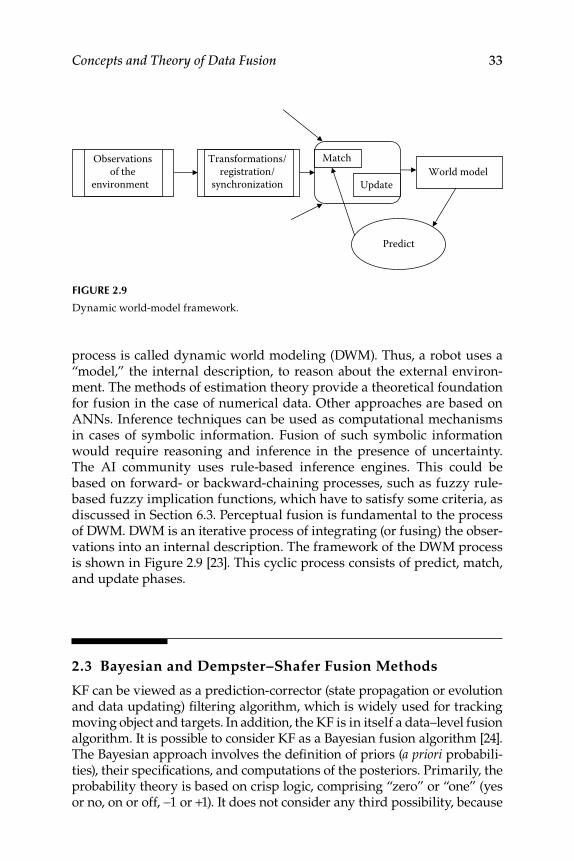
Concepts and Theory of Data Fusion 33

process is called dynamic world modeling (DWM). Thus, a robot uses a “model,” the internal description, to reason about the external environ-ment. The methods of estimation theory provide a theoretical foundation for fusion in the case of numerical data. Other approaches are based on ANNs. Inference techniques can be used as computational mechanisms in cases of symbolic information. Fusion of such symbolic information would require reasoning and inference in the presence of uncertainty. The AI community uses rule-based inference engines. This could be based on forward- or backward-chaining processes, such as fuzzy rule-based fuzzy implication functions, which have to satisfy some criteria, as discussed in Section 6.3. Perceptual fusion is fundamental to the process of DWM. DWM is an iterative process of integrating (or fusing) the obser-vations into an internal description. The framework of the DWM process is shown in Figure 2.9 [23]. This cyclic process consists of predict, match, and update phases.

2.3 Bayesian and Dempster–Shafer Fusion Methods

KF can be viewed as a prediction-corrector (state propagation or evolution and data updating) fi ltering algorithm, which is widely used for tracking moving object and targets. In addition, the KF is in itself a data–level fusion algorithm. It is possible to consider KF as a Bayesian fusion algorithm [24]. The Bayesian approach involves the defi nition of priors ( a priori probabili-ties), their specifi cations, and computations of the posteriors. Primarily, the probability theory is based on crisp logic, comprising “zero” or “one” (yes or no, on or off, −1 or +1). It does not consider any third possibility, because

FIGURE 2.9

Dynamic world-model framework.

Observationsof the

environment

Transformations/registration/

synchronization

Match

UpdateWorld model

Predict

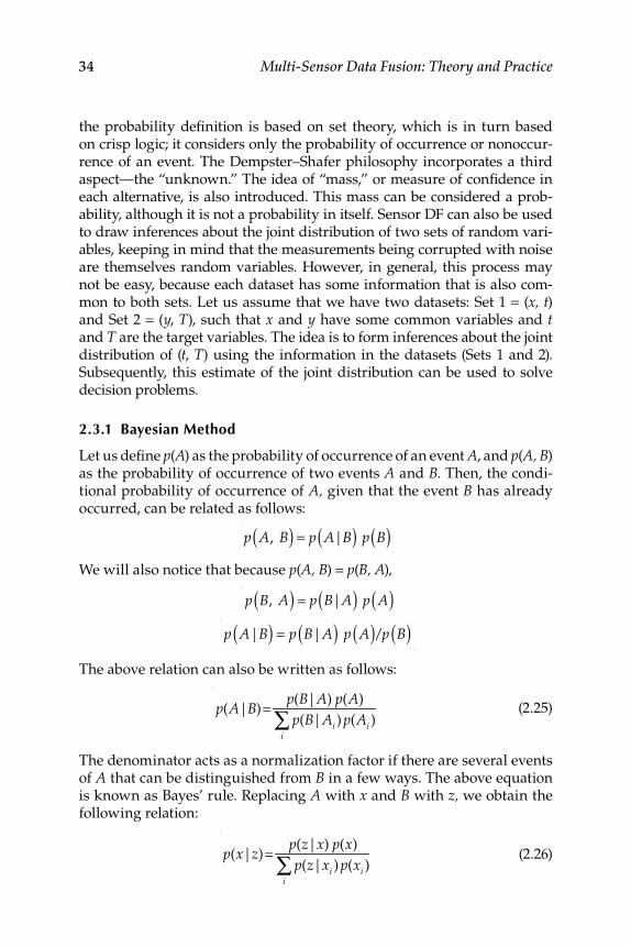
34 Multi-Sensor Data Fusion: Theory and Practice

the probability defi nition is based on set theory, which is in turn based on crisp logic; it considers only the probability of occurrence or nonoccur-rence of an event. The Dempster–Shafer philosophy incorporates a third aspect—the “unknown.” The idea of “mass,” or measure of confi dence in each alternative, is also introduced. This mass can be considered a prob-ability, although it is not a probability in itself. Sensor DF can also be used to draw inferences about the joint distribution of two sets of random vari-ables, keeping in mind that the measurements being corrupted with noise are themselves random variables. However, in general, this process may not be easy, because each dataset has some information that is also com-mon to both sets. Let us assume that we have two datasets: Set 1 = ( x, t ) and Set 2 = ( y, T ), such that x and y have some common variables and t and T are the target variables. The idea is to form inferences about the joint distribution of ( t , T ) using the information in the datasets (Sets 1 and 2). Subsequently, this estimate of the joint distribution can be used to solve decision problems.

2.3.1 Bayesian Method

Let us defi ne p ( A ) as the probability of occurrence of an event A , and p ( A, B ) as the probability of occurrence of two events A and B . Then, the condi-tional probability of occurrence of A, given that the event B has already occurred, can be related as follows:

p A, B( ) = p A|B( ) p B( )

We will also notice that because p ( A, B ) = p ( B, A ),

p B, A( ) = p B|A( ) p A( )

p A|B( ) = p B|A( ) p A( )/p B( )

The above relation can also be written as follows:

p(A|B)=p(B|A) p(A)

p(B|Ai ) p(Ai )i

∑

(2.25)

The denominator acts as a normalization factor if there are several events of A that can be distinguished from B in a few ways. The above equation is known as Bayes’ rule. Replacing A with x and B with z, we obtain the following relation:

p(x|z)=p(z|x) p(x)

p(z|xi ) p(xi )i

∑

(2.26)

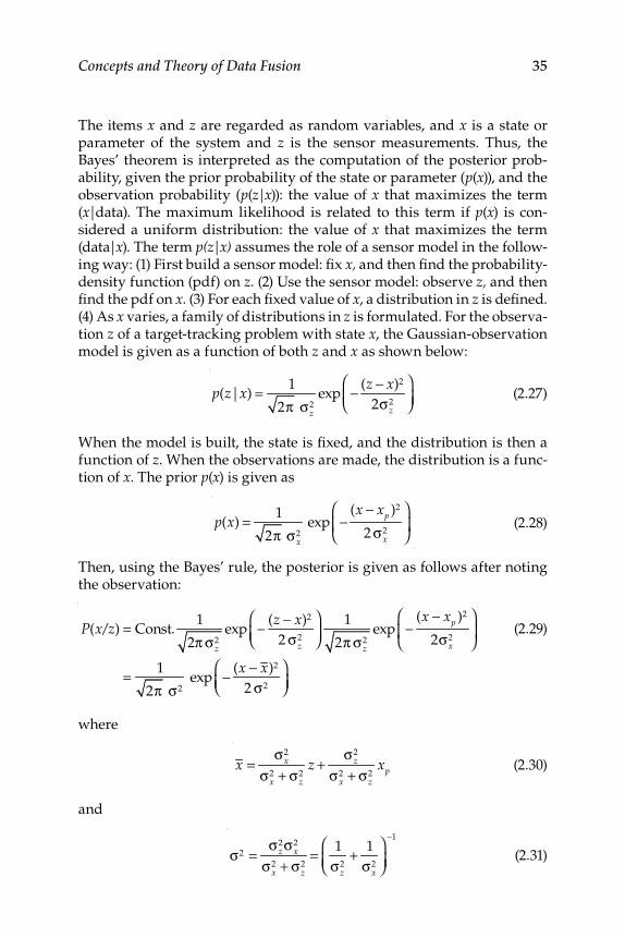
Concepts and Theory of Data Fusion 35

The items x and z are regarded as random variables, and x is a state or parameter of the system and z is the sensor measurements. Thus, the Bayes’ theorem is interpreted as the computation of the posterior prob-ability, given the prior probability of the state or parameter ( p ( x )), and the observation probability ( p ( z | x )): the value of x that maximizes the term ( x |data). The maximum likelihood is related to this term if p ( x ) is con-sidered a uniform distribution: the value of x that maximizes the term (data| x ). The term p(z|x) assumes the role of a sensor model in the follow-ing way: (1) First build a sensor model: fi x x, and then fi nd the probability-density function (pdf) on z . (2) Use the sensor model: observe z, and then fi nd the pdf on x . (3) For each fi xed value of x , a distribution in z is defi ned. (4) As x varies, a family of distributions in z is formulated. For the observa-tion z of a target-tracking problem with state x , the Gaussian-observation model is given as a function of both z and x as shown below:

p(z|x) = 1

2π σz2

exp − (z − x)2

2σz2

⎛⎝⎜

⎞⎠⎟

(2.27)

When the model is built, the state is fi xed, and the distribution is then a function of z . When the observations are made, the distribution is a func-tion of x . The prior p ( x ) is given as

p(x) = 1

2π σx2

exp −(x − xp )2

2 σx2

⎛

⎝⎜

⎞

⎠⎟

(2.28)

Then, using the Bayes’ rule, the posterior is given as follows after noting the observation:

P(x/z) = Const.1

2π σz2

exp − (z − x)2

2 σz2

⎛⎝⎜

⎞⎠⎟

1

2π σz2

exp −(x − xp )2

2σx2

⎛

⎝⎜

⎞

⎠⎟

= 1

2π σ2exp − (x − x)2

2 σ2

⎛⎝⎜

⎞⎠⎟

where

x =

σx2

σx2 + σz

2z +

σz2

σx2 + σz

2xp

(2.30)

and

σ2 =

σz2σx

2

σx2 + σz

2= 1

σz2

+ 1

σx2

⎛⎝⎜

⎞⎠⎟

−1

(2.31)

(2.29)

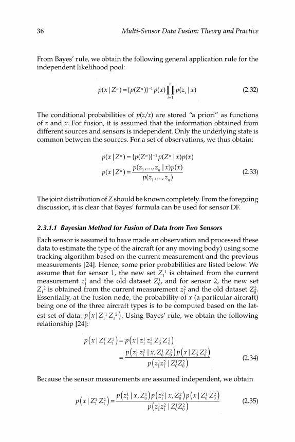
36 Multi-Sensor Data Fusion: Theory and Practice

From Bayes’ rule, we obtain the following general application rule for the independent likelihood pool:

p(x|Zn ) = {p(Zn )}−1 p(x) p(zi

i=1

n

∏ |x)

(2.32)

The conditional probabilities of p ( z / x ) are stored “a priori” as functions of z and x . For fusion, it is assumed that the information obtained from different sources and sensors is independent. Only the underlying state is common between the sources. For a set of observations, we thus obtain:

p(x|Zn ) = {p(Zn )}−1 p(Zn|x)p(x)

p(x|Zn ) =p(z

1, ..., zn|x)p(x)

p(z1, ..., zn ) (2.33)

The joint distribution of Z should be known completely. From the foregoing discussion, it is clear that Bayes’ formula can be used for sensor DF.

2.3.1.1 Bayesian Method for Fusion of Data from Two Sensors

Each sensor is assumed to have made an observation and processed these data to estimate the type of the aircraft (or any moving body) using some tracking algorithm based on the current measurement and the previous measurements [24]. Hence, some prior probabilities are listed below. We assume that for sensor 1, the new set Z

11 is obtained from the current

measurement z11 and the old dataset Z

01, and for sensor 2, the new set

Z1

2 is obtained from the current measurement z12 and the old dataset Z

02.

Essentially, at the fusion node, the probability of x (a particular aircraft) being one of the three aircraft types is to be computed based on the lat-

est set of data: p x|Z1

1 Z1

2( ) . Using Bayes’ rule, we obtain the following relationship [24]:

p x|Z11 Z

12( ) = p x|z

11 z

12 Z

01 Z

02( )

=p z

11 z

12 |x, Z

01 Z

02( ) p x|Z

01 Z

02( )

p z11z

12 |Z

01Z

02( ) (2.34)

Because the sensor measurements are assumed independent, we obtain

p x|Z11 Z

12( ) =

p z11|x, Z

01( ) p z

12|x, Z

02( ) p x|Z

01 Z

02( )

p z11z

12 |Z

01Z

02( )

(2.35)

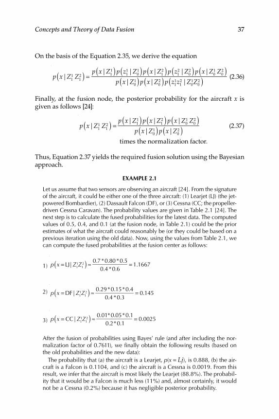
Concepts and Theory of Data Fusion 37

On the basis of the Equation 2.35, we derive the equation

p x|Z11 Z

12( ) =

p x|Z11( ) p z

11|Z

01( ) p x|Z

12( ) p z

12 |Z

02( ) p x|Z

01 Z

02( )

p x|Z01( ) p x|Z

02( ) p z

11z

12 |Z

01Z

02( ) (2.36)

Finally, at the fusion node, the posterior probability for the aircraft x is given as follows [24]:

p x|Z11 Z

12( ) =

p x|Z11( ) p x|Z

12( ) p x|Z

01 Z

02( )

p x|Z01( ) p x|Z

02( ) (2.37)

times the normalization factor.

Thus, Equation 2.37 yields the required fusion solution using the Bayesian approach.

EXAMPLE 2.1

Let us assume that two sensors are observing an aircraft [24]. From the signature of the aircraft, it could be either one of the three aircraft: (1) Learjet (LJ) (the jet-powered Bombardier), (2) Dassault Falcon (DF), or (3) Cessna (CC; the propeller-driven Cessna Caravan). The probability values are given in Table 2.1 [24]. The next step is to calculate the fused probabilities for the latest data. The computed values of 0.5, 0.4, and 0.1 (at the fusion node, in Table 2.1) could be the prior estimates of what the aircraft could reasonably be (or they could be based on a previous iteration using the old data). Now, using the values from Table 2.1, we can compute the fused probabilities at the fusion center as follows:

1) p x = LJ| Z1

1Z12( ) ≈ 0.7*0.80 *0.5

0.4 *0.6= 1.1667

2) p x = DF| Z11Z1

2( ) ≈ 0.29*0.15*0.40.4 *0.3

= 0.145

3) p x = CC| Z1

1Z12( ) ≈ 0.01*0.05*0.1

0.2*0.1= 0.0025

After the fusion of probabilities using Bayes’ rule (and after including the nor-malization factor of 0.7611), we fi nally obtain the following results (based on the old probabilities and the new data):

The probability that (a) the aircraft is a Learjet, p ( x = Lj ), is 0.888, (b) the air-craft is a Falcon is 0.1104, and (c) the aircraft is a Cessna is 0.0019. From this result, we infer that the aircraft is most likely the Learjet (88.8%). The probabil-ity that it would be a Falcon is much less (11%) and, almost certainly, it would not be a Cessna (0.2%) because it has negligible posterior probability.

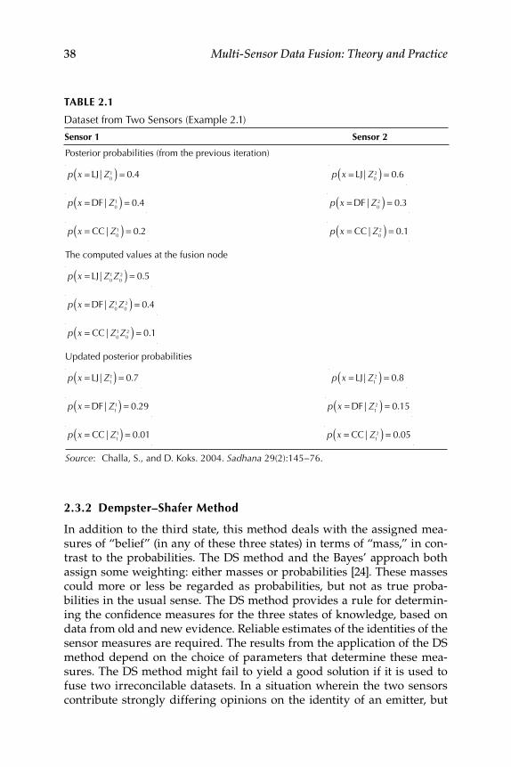
38 Multi-Sensor Data Fusion: Theory and Practice

2.3.2 Dempster–Shafer Method

In addition to the third state, this method deals with the assigned mea-sures of “belief” (in any of these three states) in terms of “mass,” in con-trast to the probabilities. The DS method and the Bayes’ approach both assign some weighting: either masses or probabilities [24]. These masses could more or less be regarded as probabilities, but not as true proba-bilities in the usual sense. The DS method provides a rule for determin-ing the confi dence measures for the three states of knowledge, based on data from old and new evidence. Reliable estimates of the identities of the sensor measures are required. The results from the application of the DS method depend on the choice of parameters that determine these mea-sures. The DS method might fail to yield a good solution if it is used to fuse two irreconcilable datasets. In a situation wherein the two sensors contribute strongly differing opinions on the identity of an emitter, but

TABLE 2.1

Dataset from Two Sensors (Example 2.1)

Sensor 1 Sensor 2

Posterior probabilities (from the previous iteration)

p x = LJ| Z0

1( ) = 0.4 p x = LJ| Z0

2( ) = 0.6

p x = DF| Z0

1( ) = 0.4 p x = DF| Z0

2( ) = 0.3

p x = CC| Z0

1( ) = 0.2 p x = CC| Z0

2( ) = 0.1

The computed values at the fusion node

p x = LJ| Z0

1 Z02( ) = 0.5

p x = DF| Z0

1 Z02( ) = 0.4

p x = CC| Z0

1 Z02( ) = 0.1

Updated posterior probabilities

p x = LJ| Z1

1( ) = 0.7 p x = LJ| Z1

2( ) = 0.8

p x = DF| Z1

1( ) = 0.29 p x = DF| Z1

2( ) = 0.15

p x = CC| Z1

1( ) = 0.01 p x = CC| Z1

2( ) = 0.05

Source: Challa, S., and D. Koks. 2004. Sadhana 29(2):145−76.

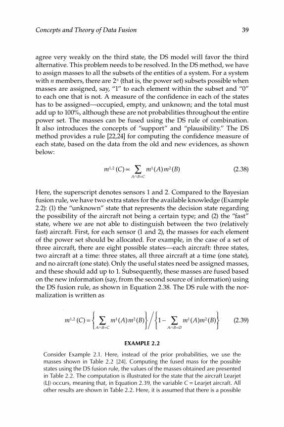
Concepts and Theory of Data Fusion 39

agree very weakly on the third state, the DS model will favor the third alternative. This problem needs to be resolved. In the DS method, we have to assign masses to all the subsets of the entities of a system. For a system with n members, there are 2n (that is, the power set) subsets possible when masses are assigned, say, “1” to each element within the subset and “0” to each one that is not. A measure of the confi dence in each of the states has to be assigned—occupied, empty, and unknown; and the total must add up to 100%, although these are not probabilities throughout the entire power set. The masses can be fused using the DS rule of combination. It also introduces the concepts of “support” and “plausibility.” The DS method provides a rule [22,24] for computing the confi dence measure of each state, based on the data from the old and new evidences, as shown below:

m1,2 (C) ∝ m1(A)m2 (B)

A∩B=C∑ (2.38)

Here, the superscript denotes sensors 1 and 2. Compared to the Bayesian fusion rule, we have two extra states for the available knowledge (Example 2.2): (1) the “unknown” state that represents the decision state regarding the possibility of the aircraft not being a certain type; and (2) the “fast” state, where we are not able to distinguish between the two (relatively fast) aircraft. First, for each sensor (1 and 2), the masses for each element of the power set should be allocated. For example, in the case of a set of three aircraft, there are eight possible states—each aircraft: three states, two aircraft at a time: three states, all three aircraft at a time (one state), and no aircraft (one state). Only the useful states need be assigned masses, and these should add up to 1. Subsequently, these masses are fused based on the new information (say, from the second source of information) using the DS fusion rule, as shown in Equation 2.38. The DS rule with the nor-malization is written as

m1,2 (C) = m1(A)m2 (B)

A∩B=C∑⎧

⎨⎩

⎫⎬⎭

1 − m1(A)m2 (B)A∩B=∅∑⎧

⎨⎩

⎫⎬⎭

(2.39)

EXAMPLE 2.2

Consider Example 2.1. Here, instead of the prior probabilities, we use the masses shown in Table 2.2 [24]. Computing the fused mass for the possible states using the DS fusion rule, the values of the masses obtained are presented in Table 2.2. The computation is illustrated for the state that the aircraft Learjet (LJ) occurs, meaning that, in Equation 2.39, the variable C = Learjet aircraft. All other results are shown in Table 2.2. Here, it is assumed that there is a possible

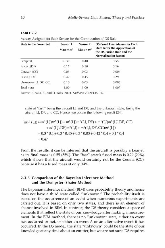
40 Multi-Sensor Data Fusion: Theory and Practice

state of “fast,” being the aircraft LL and DF, and the unknown state, being the aircraft LJ, DF, and CC. Hence, we obtain the following result [24]:

m1,2 (LJ) ∝ m1(LJ)m2 (LJ)+ m1(LJ)m2 (LJ, DF) + m1(LJ)m2 (LJ, DF, CC)

+ m1(LJ, DF)m2 (LJ)+ m1(LJ, DF, CC)m2 (LJ)

= 0.3 * 0.4 + 0.3 * 0.45 + 0.3 * 0.03 + 0.42 * 0.4 + 0.1 * 0.4

= 0.47

From the results, it can be inferred that the aircraft is possibly a Learjet, as its fi nal mass is 0.55 (55%). The “fast” state’s fused mass is 0.29 (29%), which shows that the aircraft would certainly not be the Cessna (CC), because it has a fused mass of only 0.4%.

2.3.3 Comparison of the Bayesian Inference Method and the Dempster–Shafer Method

The Bayesian inference method (BIM) uses probability theory and hence does not have a third state called “unknown.” The probability itself is based on the occurrence of an event when numerous experiments are carried out. It is based on only two states, and there is an element of chance involved in BIM. In contrast, the DS theory considers a space of elements that refl ect the state of our knowledge after making a measure-ment. In the BIM method, there is no “unknown” state; either an event has occurred or not, or either an event A or an alternative event B has occurred. In the DS model, the state “unknown” could be the state of our knowledge at any time about an emitter, but we are not sure. DS requires

TABLE 2.2

Masses Assigned for Each Sensor for the Computation of DS Rule

State in the Power Set Sensor 1 Sensor 2 DS-Fused Final Masses for Each State (after the Application of the DS-Fusion Rule and the Normalization Factor)

Mass = m1 Mass = m2

Learjet (LJ) 0.30 0.40 0.55

Falcon (DF) 0.15 0.10 0.16

Caravan (CC) 0.03 0.02 0.004

Fast (LJ, DF) 0.42 0.45 0.29

Unknown (LJ, DK, CC) 0.10 0.03 0.003

Total mass 1.00 1.00 1.007

Source: Challa, S., and D. Koks. 2004. Sadhana 29(2):145−76.

Concepts and Theory of Data Fusion 41

the masses to be assigned in a meaningful way to all the states, whereas BIM requires the priors (probabilities) to be assigned. However, a pre-liminary assignment of masses could be required to refl ect the initial knowledge of the system. The DS model allows computation of support and plausibility, in addition to involving more computations compared to the BIM model.

2.4 Entropy-Based Sensor Data Fusion Approach

It is important for a sensor NW to perform effi ciently in certain diffi cult environments. The NW should process available information effi ciently and share it such that decision accuracies are enhanced. One interesting approach is to measure the value of information (VOI) obtained from the various sensors, and to then fuse the information if the value (a gain involving signifi cant importance and appreciation) is added in terms of the decision accuracy (DA) [25,26]. The concept is based on the information-theoretic (metric entropy) measure and related concepts. The DF here is conditioned upon whether the VOI has improved the DA. In certain other situations, we have two aspects to consider in a single image, such as the spatial resolution and the spectral resolution (of the imaging sensor or system). A high spatial resolution might be accompanied by low spec-tral information, and high spectral resolution might be accompanied by low spatial resolution. To obtain high spatial and spectral resolutions, specifi c methods of image DF need to be applied. This is a useful pro-cess for merging similar-sensor and multisensor images to enhance the image information. For this purpose, a metric system based on entropy can be useful. Entropy perceives information as a frequency of change in images (the digital numbers). It is unfortunate that, in some literature, entropy is used directly as information, but the context clears the ambi-guity in presentation. In fact, when a new set of data is added and used for analysis and inferences, then the new entropy (uncertainty) will be reduced compared to the old entropy (uncertainty), and the difference will be the gain in the information. The use of entropy must be viewed in this context.

2.4.1 Definition of Information

In 1948, Claude Shannon applied the probabilistic concept in modeling message communications, with the proposal that a particular message is one element (possibility one) from a set of all possible messages. Given the fi nite set of the number of messages, any monotonic function of this number can be used as a measure of the information when one message is

42 Multi-Sensor Data Fusion: Theory and Practice

chosen from this set. The information is modeled as a probabilistic process. It is essential to know the probability of each message occurring, the inten-tion being to isolate one message from all of the possible messages (in a set). Thus, the occurrence of this random event x is the probability p ( x ) of the message. The I ( x ) is the self-information of x , and this is the inverse of the probability, because if the event x always occurs, then p ( x ) = 1, and no new information can be transferred.

I(x) = log1

p(x)= − log{p(x)} (2.40)

The above defi nition of information is intuitively appealing from an engi-neering viewpoint. The average self-information in the set of messages with N outputs will be [25]

I(x) = −N p(x

1) log{p(x

1)} − N p(x

2) log{p(x

2)}, ..., N p(xn )log({p(xn )}) (2.41)

Then, the average information per source output is represented by the following equation:

H = −N p(xi )

i=1

n

∑ log{p(xi )} (2.42)

Here, H is also known as Shannon’s entropy. However, in general, the value of N is set to 1, and hence we obtain the following relation using the natural logarithm:

H = − p(xi )

i=1

n

∑ ln2{p(xi )} (2.43)

Shannon introduced the mathematical concept of information and estab-lished a technical value and a meaning of information. From the above development, we can see that the entropy (somewhat directly related to the covariance) or uncertainty of a random variable X having a probabili-ty-density function p ( x ) is defi ned as

H(x) = −E x {log p(x)} (2.44)

It is the −ve expected value of the logarithm of the pdf of the random vari-able X . Entropy can be roughly thought of as a measure of disorder or lack of information. Now, let H(β) = − E β[log p(β)], the entropy before collecting

Concepts and Theory of Data Fusion 43

data “ z ,” and p ( β ) the prior density function of β , a specifi c parameter of interest. When the data z is collected, we have the following relation:

H(β|z) = −Eβ/z {log p(β|z)} (2.45)

The measure of the average amount of information provided or gained by the experiment with data z on the parameter β is provided by the following relationship:

I = H(β) − E z {H(β, z)} (2.46)

This is the “mean information” in z about β . We note that entropy implies the dispersion or covariance of the density function and, hence, the uncer-tainty. Thus, the information I is perceived as the difference between the prior uncertainty (which is generally large) and the “expected” posterior uncertainty (which is now reduced due to the new data adding some information about the parameter or variable of interest). This indicates that due to experimentation, collection, and the use of data z , the (poste-rior) uncertainty (which is expected to reduce) is reduced and, informa-tion is gained. Thus, the information is a nonnegative measure, and it is zero if p (z,β) =p(z) gp(β); i.e., if the data are independent of the parameters, which implies that the data does not contain any information regarding that specifi c parameter.

2.4.2 Mutual Information

The information could be in the form of features for classifi cation or data for detection of an object. Let H ( x ) be the entropy of the observed event, and let z be a new event with its uncertainty (entropy) as H ( z ). Then, we can evaluate the uncertainty of x after the event z has occurred and incor-porate it to compute the new entropy:

H(x|z) = H(x, z) − H(z) (2.47)

This conditional entropy H ( x | z ) signifi es the amount of uncertainty remaining about x after z has been observed or accounted for. Thus, if the uncertainty is reduced, information has been gained by observing and incorporating z , the new information. The mutual information I ( x , z ) is a measure of the uncertainty after observing and incorporating z and can be represented as follows:

I(x, z) = H(x) − H(x|z) (2.48)

44 Multi-Sensor Data Fusion: Theory and Practice

Thus, the VOI is useful when we want to assess the information available from multiple sensors on a single node or from different sensors from neighboring nodes.

2.4.3 Entropy in the Context of an Image

Information-content quantifi cation can be similarly applied to the infor-mation regarding an image (as digital numbers and related attributes such as the pixels of an image). Shannon’s formula is modifi ed as follows [25,26]:

H = − d(i)

i=1

Ng

∑ ln2{ d (i)} (2.49)

Here, Ng

is the number of the gray level of a histogram of the image. This histogram range, for an 8-bit image, is between 0 and 255. The variable d ( i ) is the normalized frequency of occurrence of each gray level, and hence the average information content is estimated in units of bit per pixel. It should be noted here that the average information content of the image is not affected by the size of the image or by the pattern of gray levels. How-ever, it is affected by the frequency of each gray level.

2.4.4 Image-Noise Index

For image fusion, the concept of entropy can be used to estimate the change in quantity of information between the original images (called the parent images) and the new images (called the child images) obtained by fusion of two parent images (from two image-sensing devices). The procedure for computation of the image-noise index (INI) is explained next [26]. In the forward pass, the images are fused by a chosen method, and the fused image is obtained. This fused image is restored in the reverse pass to its original condition (i.e., the parent image) by using the reverse process, and the entropy of the restored image is estimated. To bring the fused image to its original condition, the original spatial-resolution value of the multispec-tral image is substituted in the reverse process. Because we know the three entropy values ( a , b , and c ) of the original image, the fused image, and the restored image, respectively, we can easily determine the INI. The quantity | a − c | represents the unwanted information and, hence, the noise. The dif-ference ( b − a ) represents the increase in information, which could be useful information, the noise, or both. Thus, the INI is defi ned as follows [26]:

INI = (b − a) − (|a − c|)

|a − c|= (b − c)

|a − c|− 1 (2.50)

Concepts and Theory of Data Fusion 45

The numerator of the fi rst term is the amount of useful information added (the signal). Thus, the INI gives the incremental signal-to-noise ratio (SNR) of the fusion process.

2.5 Sensor Modeling, Sensor Management, and

Information Pooling

Recent advances in electronics, computer science and engineering, and optics have resulted in a massive increase in the types of sensors available for use in autonomous systems [27–29]. Automated systems must be able to react to changes in their environment to be effective, and these systems must therefore rely on sensors for information about their environment. The sensors provide dependable interfaces between an often ill-defi ned and chaotic reality and a computer with a data-acquisition system. Sen-sors can handle data only when they are within specifi ed bounds and are presented in a precise format for ease of understanding and inter-pretation. Often sensors are complex and might have limited resolution and reliability. In complex systems, the sensors do not necessarily corre-spond to a single concrete sensor. A sensor might have some preprocess-ing built-in unit or some logic or intelligence- processing unit built within the sensor system. The readings from the sensors can be fused to create one abstract sensor.

Sensors that correspond to only one concrete sensor are called “simple sensors,” and sensors made up of several concrete sensors are called “sen-sor NWs,” and are created from many simple sensors. After fusion, the data from a sensor NW can be treated as if the data originated from a simple sensor. Sensor NWs can have many different levels of complexity, architec-tures, and confi gurations. These architectures have different requirements for data communication and have varying computational complexities. The performance of sensors is measured in terms of accuracy, repeatabil-ity, linearity, sensitivity, resolution, reliability, and the range it can handle. The sensor output could be a continuous signal, digital signal, frequency output, amplitude, pulse modulated, and so on.

2.5.1 Sensor Types and Classification

Active sensors inject varying types of signals into their environments and then measure the interaction of the signal with the environment, e.g., radar, sonar, active far (AF) infrared (IR) sensor, an active optical-seam tracker, and an active computer-vision system. These sensors require external power to operate. The signal being measured is thus modifi ed by the sensor

46 Multi-Sensor Data Fusion: Theory and Practice

to produce an output signal. These sensors are also called parametric sen-sors, e.g., in a thermistor, a change of resistance occurs due to a change in the temperature. The properties of the sensor can change in response to an external signal. Passive sensors simply record the energy or signals already present in the system’s environment, e.g., thermometers, video cameras, and IR cameras. The energy of the input stimulus is converted by the sen-sor or transducer into output energy without the need for an additional power source or injection of energy into the sensor, e.g., a thermocouple, a piezoelectric sensor, a pyroelectric detector, and passive IR sensor.

2.5.1.1 Sensor Technology

There are mainly two types of sensor technologies [29]: (1) internal state sensors (ISSs), and (2) external navigational state sensors (ENSS).

ISSs [29] measure the internal states of the system; for example, in the case of a robot, the velocity, attitude and bearings, accelerations, current, voltage, temperature, pressure, balance, and so on are recorded so that the static and dynamic stability of the robot can be monitored and main-tained, and potential failure situations can be detected and avoided. Some examples of such sensors are potentiometers, tachometers, accelerometers, and optical encoders. These interoceptive sensors inform the body of its own state. They are mainly related to the problems of internal diagnosis and fault detection. Two types of ISSs are described in the following two paragraphs.

Contact-state sensors (CSSs) involve direct physical contact with the objects of interest; e.g., microswitches and touch, force, and tactile poten-tiometers [29]. Contact sensors are used to handle objects, reach a specifi c location, and protect a robot from colliding with obstacles. These are rela-tively inexpensive, have a quick response, and are easy to construct and operate. The tactile sensors are magnetic, capacitive, and include piezo-electric technology. A binary tactile sensor can be used for detecting the presence or absence of touch, and a 2D tactile sensor can provide informa-tion regarding the size, shape, and position of an object. CSSs have limited life span because of frequent contacts with objects.

Non-contact state sensors (NCSSs) [29] are synchros, resolvers, com-passes, accelerometers, gyroscopes, and optic encoders. Synchros and resolvers are rotating electromechanical devices that measure the angular position information; these devices are normally large and heavy. Gyros are mechanical and optical devices and are used to maintain the stabil-ity and attitude of robotic systems (useful in unmanned fl ying robots, underwater vehicles, space robots that navigate in a 3D environment, unmanned aerial vehicles [UAVs], and so on). Gyroscopes can be used to measure the movement of a system relative to its frame of reference. Com-passes, gyroscopes, and encoders are generally combined into an inertial

Concepts and Theory of Data Fusion 47

navigation sensor (INS), which is used to estimate the trajectory followed by an object. Mechanical gyros operate on the basis of conservation of momentum, whereas optical gyros have no moving parts. The absolute optic encoders are used to measure and control the angle of the steering wheel during the path control of a wheeled robot. The incremental optic encoders are used for measuring and controlling motor speed and accel-eration in a mobile robot.

ENSSs monitor the system’s geometry and dynamics in relation to its tasks and environment, e.g., proximity devices, strain gauges, sonar (ultrasonic range sensor), and pressure and electromagnetic (EM) sen-sors [29]. External navigational sensors measure environmental features such as range, color, gap, road width, room size, and object shape. These are used for correcting the errors in the world model, detecting environ-mental changes, and avoiding unexpected obstacles. The exteroceptive sensors deal with the external world. The sense of “balance” can be moni-tored mechanically using gyroscopes. The system’s joint positions can be sensed by the mechanical system using encoders. Both balance and joint positions can be handled by the INS to some extent.

Nonvision-based navigation sensors (NVBENSS) [29] are force and magnetic sensors, which are passive navigation sensors. They do not gen-erate EM waves, are reliable, and produce little noise. The force sensor can be used to monitor whether there is an object in contact with the robot for avoiding collision, e.g., a full cover with a force-detecting bumper can be implemented on a cylindrical robot for safe operation. An actu-ated whisker can be used to measure the profi les of the contacted objects for object identifi cation and obstacle avoidance. Sound (energy), smell, IR radiation, optics, laser, radio frequency (RF), satellites, and radars are other NVBENSS sensors. The data measured by the active sensors are the refl ection of either the changes in emitted-energy properties, such as the frequency and phase, or simple time-of-fl ight calculation. These sensors provide one-dimensional data at a high rate and are useful for following the path, reaching a goal, avoiding obstacles, and mapping an environ-ment. Sonar (ultrasonic) sensors have long wavelengths.

Global positioning systems (GPS) provide a robust alternative to many other methods of navigation. Satellite beacons are used to determine an object’s position anywhere on the earth. Other beacon systems are used in transportation NWs, especially in maritime and aviation systems. GPS and RF systems are widely used in robot localization and tracking of objects and humans, using the services of 24 satellites at a height of 6900 nautical miles. The absolute 3D position of any GPS receiver can be determined using a triangulation method. Time-of-fl ight radio signals, which are uniquely coded and transmitted from the satellites, are routinely used worldwide. Problems with GPS include incorrect time synchronization between the satellite and receiver, precise real-time location of the satellites, EM noise,

48 Multi-Sensor Data Fusion: Theory and Practice

and other interferences. Differential GPS (DGPS) provides much more precise data than the GPS alone regarding the positions of the objects. The integration of data from the GPS and other INSs leads to fusion of data that reduces the effects of uncertainties. An odor- detection system allows a robot to follow trails of volatile chemicals laid on the fl oor. The sensor uses controlled fl ows of air to draw odor-laden air over the sensor crystal to increase the speed of its response.

Vision-based ENSSs mimic human eyes. The visual information obtained from a vision sensor proceeds through three processing stages [29]: image registration and transformation, image segmentation and analysis, and image interpretation (and image fusion, if included in this process)—a diffi cult task to achieve in real-time. Charge-coupled devices (CCDs), both active and passive, can be used. Active CCDs use structured lighting to illuminate the scene and enhance the area of interest to make image- processing more effi cient; the data in the enhanced area only is processed, projecting a pattern of light strips onto the scene, whereas the depth infor-mation can be obtained by looking for discontinuities or deformation in the resulting line image. Passive vision-based sensors work under normal ambient illumination and are used in wheeled, legged, tracked, under-water, and fl ying robots. They are mainly used for object and landmark recognition, line-following, and goal-seeking tasks.

2.5.1.2 Other Sensors and their Important Features and Usages

Many other sensors are equally important [4,29]. Smell and taste involve measuring the concentration of specifi c chemicals in the environment. Odor sensing detects chemical compounds and estimates their density within an area. Odors from different materials have different particle compositions, and hence have different locations in the spectra. Auto-mated systems can sense odors by using EM radiation in the process of spectroscopy. Recent advances in fi ber optics have produced fi ber-optic probes that are capable of detecting biochemical agents.

Touch involves measuring items through physical contact, and in auto-mated systems, this is usually carried out using pneumatics or whiskers. Tactile sensing can be accomplished by numerous methods: the simplest sensors detect the presence or lack of an object; e.g., whiskers that are long, light, and relatively stiff protrude from a system or a body, similar to the whiskers in our nostrils and inner ears. When a whisker touches an object, the whisker is displaced. A sensor at the base of the whisker senses this movement and signals the presence of an object. The ambient EM radiation that has been refl ected from the object can be detected and used for measurements.

IR cameras capture IR radiation, whose wavelength is longer than visible light. Forward-looking IR (FLIR) sensors sense differences in the

Concepts and Theory of Data Fusion 49

heat of objects and construct images from that information. These sen-sors are useful in night-vision applications. Radar is an EM system for the detection and location of objects, which consists of transmitting antennae emitting EM radiation generated by an oscillator, receiving antennae, and an energy-detecting device or receiver. A portion of the transmitted signal is refl ected by a target and reradiated in all directions. This refl ected EM radiation (the returned energy) is collected by the receiving antennae and is delivered to a receiver, where it is processed. From the processing of this data, the object is detected and its location and relative velocity are measured by ranging (which is proportional to the speed of light times the total fl y-around time/2). The direction or angular position is deter-mined from the direction of the arrival (Section 11.3) of the returned wave front (the acoustic wave for sonar systems). If there is a relative motion between the detected target and the radar, the shift in the carrier fre-quency of the refl ected wave—the Doppler effect—gives the measure of the relative velocity of the object. These measurements are very useful in target tracking.

Microwave radars use wavelengths longer than infrared radiation, and are insensitive to interference from clouds and inclement weather. They are better in terms of detection range and immunity to attenuation caused by atmosphere. However, their capabilities for classifi cation and identifi -cation are not very good. Laser ranging systems (laser radar or LADAR) provide images of very accurate depth from a scene. The “identify friend-or-foe” function is used to identify the origin of an aircraft. Apart from these, sound navigation and ranging is an established technology that is approximately equivalent to radar. A sound wave is transmitted in space, and its return signal is measured. By measuring the time needed for the signal to return, the distance of an object from the sensor can be estimated. The velocity of the object relative to the sensor can be estimated using the frequency shift of the returned signal in comparison to the original signal (Doppler shift). These sensors have been developed for both underwater and terrestrial applications, such as detection of submarines, manufac-ture of self-focusing cameras, and navigation systems for autonomous robotics.

Bumpers are large protuberances from the system, which, when touched, signal contact with an object through an electrical switch. Light-emitting diodes can be used as refl ecting sensors to detect objects in the immediate neighborhood. Proprioceptive sensors indicate a sys-tem’s absolute position or the positions of the system’s joints. The posi-tions of a system’s joints can be determined by using the direct-drive mechanism, as in a stepper motor, or with an optical encoder attached to the joint. By observing the motion of the encoder, the relative posi-tion of a wheel, joint, or track in relation to the rest of the system can be calculated.

50 Multi-Sensor Data Fusion: Theory and Practice

An EM-induction (EMI) sensor is used for metal detection. The idea is to detect the secondary magnetic fi eld produced by the eddy currents induced in the to-be-detected metal (say, hidden underground) by a time-varying primary magnetic fi eld, in the frequency range of a few tens of kHz [30]. EMI sensors can be used to detect both ferrous and nonferrous metallic objects. If multiple targets (for example, many metal pieces or devices present underground and considered target objects) must be detected, then the method of data association can be used. The intensity of the received fi eld depends on the depth of the target hidden under-ground. Thus, the attenuation of the received fi eld would be much higher if the target is deep down. EMI sensors can be used in a variety of modes, such as (1) high-sensitivity search, to detect even small quantities of metal; (2) low-sensitivity search, which has a low probability of detection amidst metallic clutter; and (3) shape search, where the features measured are the metal content and the shape [30].

Ground-penetrating radars (GPRs) detect buried objects by emitting radio waves into the ground. The refl ected waves are analyzed. The GPR system has antennae to emit a signal and receive the return signal and a computerized signal-processing system [30]. The frequency of the radio wave is the major control parameter, because the scale or level of detection is proportional to the wavelength of the input signal, i.e., if the wavelength decreases (and consequently, the frequency increases), the quality of the image is enhanced. Signal-processing algorithms also play an important role because they are used for fi ltering out the clutter signals. The GPR system can build a 3D image of the ground zone for detection. GPRs can be used in three modes as follows: (1) depth search—the operating fre-quency is maintained low to penetrate the ground at the greatest possible depth; (2) resolution search—the information from the fi rst mode is used to tune the operating frequency for obtaining the best possible resolution for the image (and shape and size of target); and (3) anti-ground bounce-effect search—the frequency is set to a very high value to overcome the masking effect of the ground-air discontinuity, and this mode is suitable for both surface and shallow targets. Many other features of GPR are detailed in a study by Vaghi [30].

In contrast to the thermal-detection methods that exploit the varia-tions in temperatures, IR sensors detect anomalous variations in the EM radiation refl ected by the object under detection. IR sensors are also lightweight. The quality of the IR images depends on the time of the day, weather, vegetation cover, and so on. The airborne IR sensor can procure images of the ground from a high standoff distance. The IR sensor can be used in three modes, including (1) searching for shallow buried mines; (2) searching for surface mines; and (3) achieving maximum depth of detection [30].

Concepts and Theory of Data Fusion 51

2.5.1.3 Features of Sensors

Different sensors have different characteristics, and it is important for the DF community to know the specifi c features of the sensors that are needed for primary sensing purposes and subsequent DF performance requirements. We describe some important aspects of the sensor types and their relations to the type of measurement and state determination [4,29].

From radars, we obtain two basic measurements, radar cross-section (RCS) frequency and time, and from these we derive the range, azimuth, elevation, and range-rate (Doppler effect) information. These derived data are in turn used in a state-estimation algorithm to fi nally determine the position, velocity, and acceleration time histories of a moving object accu-rately. We can determine of a limited amount of target ID information (identifi cation mark or some similar feature) from the RCS, size, and shape of the target in limited cases. From the radar homing and warning sys-tem, we initially detect the RF intensity, and then we derive the direction, which in turn is used to determine the identity of the target. For example, we get a warning by illumination from the missile-guidance radar. From a synthetic aperture radar, the coherent RCS, shape, size, and direction of the target, and ultimately, the identity of the target are determined. This methodology gives enhanced radar resolution through coherent process-ing using stable or moving antenna. The signature format is a 2D range and cross-range refl ectivity image. The useful features are size, aspect ratio, and number and locations of the scatterers.

From the IR recordings, we obtain the pixel intensity and color of the tar-get and spectral data. The derived information is location, size, shape, and temperature of the object, which fi nally yield the position and identity of the object. This is dependable for ID based on spectral data but not effi cient for determination of the position and velocity of the target. From the IR warning system, we primarily detect the IR intensity and subsequently, the direc-tion and identity of the object. This generates a warning that the heat source is approaching the observer. A laser-warning system records the intensity, which is used to determine the identity of the object. The signature formats for the laser radar are the 3D refl ectivity image, Doppler modulation (vibra-tion), and the 2D velocity image. The useful features are size, 3D shape, scat-ter locations, propulsion, structural features, skin frequencies, and spatial distribution of the moving components.

Using microwave radar, we obtain Doppler modulation 2D (range-cross range) refl ectivity images. The useful features are velocity, propulsion frequencies, line widths, size, aspect ratio, and number and location of scatterers. A millimeter wave radar (MMWR)–type sensor yields the 1D refl ectivity profi le, 1D or 2D polarization image, and Doppler modula-tion as the signatures. The useful features are the distribution and range

52 Multi-Sensor Data Fusion: Theory and Practice

extent of scatter number, locations of the odd and even bounce-scatterers, propulsion frequencies, and line widths (rpm, blade passing, and tread slapping).

The signature format of an RF interferometer is a spectrum- and time- dependent microwave emission. Its useful features are frequency, fre-quency modulation, amplitude modulation, pulse duration, and pulse intervals. The signature format of the thermal image is a 2D thermal image, and the useful features are shape (perimeter and area, aspect ratio, moments), texture, maximum and minimum emission, number and loca-tion of hot spots, and context. The MMWR is placed midway between microwave sensors and electro-optical tracking systems (EOTs). They have a smaller size, better resolution, and higher level of immunity to the effect of the atmospheric attenuation.

An electro-optical system gives intensity and color to the pixel-image, which are used for determination of the location, size, and shape of the object, and ultimately, the position and identity of the object. EOTs are superior in terms of classifi cation and identifi cation of the objects. They have a much higher resolution but are affected by atmospheric attenu-ation. Their data-processing demands are relatively high. Electronic- support measures yield amplitude, frequency, and time, which are further used for deriving SNR, polarization, and pulse shape to fi nally estimate the position, velocity, and identity of the target, providing both general and specifi c emitter IDs. An acoustic sensor’s signature format is the spec-trum- and time-dependence of the acoustic emission, and its useful fea-tures are the propulsion frequencies, harmonics, frequency ratios, pump and generator frequencies, and peculiar noise sources. We obtain a 2D refl ectivity (contrast) image. The useful features are shape, texture, inter-nal structure, and context.

2.5.1.4 Sensor Characteristics

It is also important to know the characteristics of various sensors. These characteristics are recounted below [4,29]:

1. Detection performance: false alarm rate, detection probabilities, and ranges for the calibrated target characteristics in a given noisy background.

2. Spatial and temporal resolution: ability to distinguish between two or more targets that are very close to each other in space or time.

3. Spatial coverage: spatial volume encompassed by the sensor. For scanning sensors, this may be described by the instantaneous fi eld-of-view (FOV), the scan-pattern volume, and the total fi eld-of-regard achievable by moving the scan pattern.

Concepts and Theory of Data Fusion 53

4. Detection and tracking modes: search and tracking modes undertaken are (a) starting or scanning, (b) single or multiple target tracking, and (c) single or multimode (track-while-scan and stare).

5. Target revisit rates: rate at which a specifi c target is revisited by the sensor to carry out a sample measurement.

6. Measurement accuracy: accuracy of sensor measurements in terms of statistics.

7. Measurement dimensionality: number of measurement vari-ables (range, range rate, and spectral features) between the target categories.

8. Hard vs. soft data: sensor outputs either as hard-decision (thresh-old) reports or as preprocessed reports with quantitative mea-sures of evidence for possible decision hypothesis.

9. Detection and track reporting: sensor reports each individual tar-get detection or maintains a time-sequence representation (track) of the target’s behavior.

2.5.2 Sensor Management

Several sensor NW–based systems have increased functionality and are characterized by a high degree of autonomy, reconfi gurability, and redun-dancy [30]. The sensor can be mounted on a platform and used in various modes. When the sensors move on platforms that are either teleoperated or autonomous, the movements of the sensors should be coordinated to align them to the required positions. Hence, the goals of sensor manage-ment are to provide high-level decisions and coordinate the movement of the sensors. This might need real-time information about the system’s state. Certain criteria and objectives need to be defi ned, so that decision making algorithms can be used to decide the future strategy of the sensor NW. The decisions could analyze the following questions: (1) where the platform carrying the sensors should move; (2) how the sensors should be utilized; and (3) what measurements would be needed.

A typical sensor-management problem could be very complex [30]: (1) collecting information from all the subsystems (sensors, platforms, and targets), which could be heterogeneous and distributed; and (2) com-bining this information to obtain an integrated approach for the fi nal decision making process. One approach is to model all the subsystems and their interactions, using graphical model formalism for this purpose [30]. This approach combines probability and graph theories and can lead to a stochastic adaptive algorithm for sensor management. A typical sen-sor NW management scenario could be (1) static or dynamic, coopera-tive or noncooperative targets; (2) some environmental factors that could

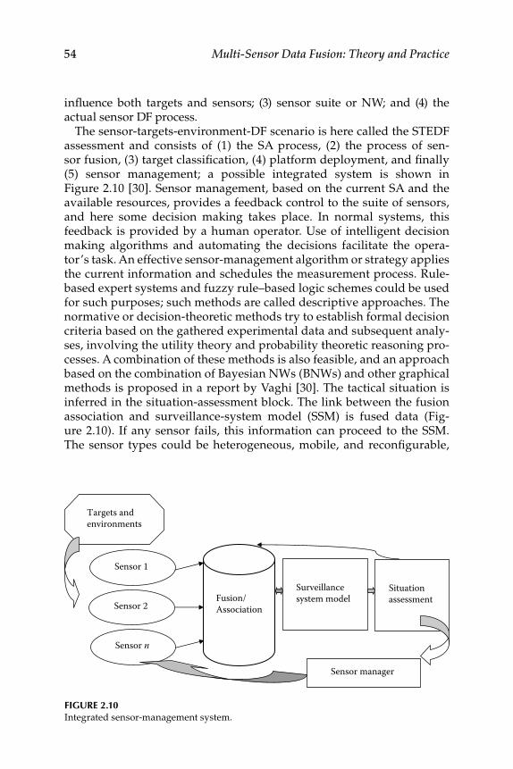
54 Multi-Sensor Data Fusion: Theory and Practice

infl uence both targets and sensors; (3) sensor suite or NW; and (4) the actual sensor DF process.

The sensor-targets-environment-DF scenario is here called the STEDF assessment and consists of (1) the SA process, (2) the process of sen-sor fusion, (3) target classifi cation, (4) platform deployment, and fi nally (5) sensor management; a possible integrated system is shown in Figure 2.10 [30]. Sensor management, based on the current SA and the available resources, provides a feedback control to the suite of sensors, and here some decision making takes place. In normal systems, this feedback is provided by a human operator. Use of intelligent decision making algorithms and automating the decisions facilitate the opera-tor’s task. An effective sensor-management algorithm or strategy applies the current information and schedules the measurement process. Rule-based expert systems and fuzzy rule–based logic schemes could be used for such purposes; such methods are called descriptive approaches. The normative or decision-theoretic methods try to establish formal decision criteria based on the gathered experimental data and subsequent analy-ses, involving the utility theory and probability theoretic reasoning pro-cesses. A combination of these methods is also feasible, and an approach based on the combination of Bayesian NWs (BNWs) and other graphical methods is proposed in a report by Vaghi [30]. The tactical situation is inferred in the situation-assessment block. The link between the fusion association and surveillance-system model (SSM) is fused data (Fig-ure 2.10). If any sensor fails, this information can proceed to the SSM. The sensor types could be heterogeneous, mobile, and reconfi gurable,

FIGURE 2.10 Integrated sensor-management system.

Sensor 1

Sensor 2

Sensor n

Fusion/Association

Targets andenvironments

Surveillancesystem model

Situationassessment

Sensor manager

Concepts and Theory of Data Fusion 55

and the target types could be simple, maneuvering, heterogeneous, or enclosed in a clutter.

2.5.2.1 Sensor Modeling

Sensors have varying accuracies and might not provide one single accu-rate value for a physical variable. This is not the case with inherently very accurate and high-precision sensors, but these sensors are very costly. Even if a sensor could deliver this type of reading, the physical values being measured generally vary statistically over a period of time and will be affected by measurement noises or errors. A sensor read-ing that covers a fi nite period would thus have to return a range of val-ues, rather than one number, to accurately represent the environment; thus, limited accuracy is a factor in all measurement-data processing. Data representations in common use have upper and lower bounds for the values that can be represented and a maximum number of digits of accuracy; if these limits on accuracy are not handled properly, important information can be lost or the results of calculations can be greatly in error. There is a possibility that a sensor might fail during the system’s lifetime or may temporarily give inaccurate readings for various rea-sons. Regardless of how well the systems are designed, the components will eventually deteriorate or stop working perfectly. Engineers and analysts must try to minimize the impact of such component failures through proper design procedures and decisions. In addition to the nor-mal wear and tear, there are limitations to the general capabilities of any component. This is especially true when the system is placed in hostile and/or noisy environments, such as nuclear reactors, battlefi elds, and outer space.

Mathematical models of the activities of these sensors can be used for characterization of the sensors and their data. Algorithms that handle sen-sor data effi ciently and accurately can be developed, and these algorithms should be effi cient in that (1) they extract the maximum information from the sensors; (2) they avoid making wrong and absurd conclusions based on faulty data; and (3) they do not waste costly system resources. The mathematical model of the sensors can be subsequently derived. A sensor can be represented as a mathematical function with two arguments, viz ., the environment and time, as follows:

S(E, t) = {V(t), e(t)} (2.51)

Here, E is an abstract entity that contains several physical measurable attri-butes, and S is a function that maps the environment to numeric values. These attributes can be continuous-valued (temperature, velocity, range, and so on), Boolean (presence of a vehicle, temperature > given limit, and

56 Multi-Sensor Data Fusion: Theory and Practice

so on), integer-valued (such as number of aircraft, tanks, and number of persons in a queue), and so on. The values recorded will change over time, because the system’s environment also changes over time. Assume V is a point in an n -dimensional space and is affected by some uncertainty. Knowing everything about the sensor in use and the measured signal, as much as possible a priori , would help in the fusion process because of the following relationship between the measurement and the object’s state: measurements = sensor’s dynamic math model times the state (or parameter) + noise; or,

z = Hx + v (2.52)

Here, the aim is to estimate the state vector x based on y , and hence any information regarding H and the statistics of v, such as the sensor type, “range band,” and “range” of the measurement signal, would help in the estimation of x . The scale factor and bias errors can be related as follows:

z(measured data) = ay + bias (2.53)

Here, a is the scale factor. General aspects regarding the preprocessing of measurement considering the sensor fi lter are (1) fi lter dynamics, because a low-pass analog fi lter might have been used to remove the high- frequency noise, (2) sensor-mounting errors (rate gyros detect signals from other axes, if misaligned), and (3) the position of the linear accelerometer, which must be known. All of the above aspects will help the analyst understand the performance results of the DF system or to correct the data at the out-set itself. The analyst should know as much as possible of the entire chain, including how the data get to him/her from the transducer or sensors, because the screening, editing of the data, and signal processing, together with system identifi cation, are important functions to be performed to obtain very accurate results from the DF systems. The important aim of sensor modeling is to incorporate the dominant modes of the sensor dynamics, if any, into the modeling effort for DF systems, e.g., in state models used in the KF. An SSM could be represented as a nonlinear state-space model, as shown below:

x(t + 1) = f (x(t), u(t)) (2.54)

Here, x, the state vector, consists of the variables related to sensors, plat-forms, targets, and environmental conditions; u is the decision vector, representing controllable inputs (or decisions in the surveillance sys-tem, e.g., sensor allocation and platform deployment). Thus, the SSM is

Concepts and Theory of Data Fusion 57

a stochastic model. The system output y contains the measurements, all control elements, and decisions. The platform states and the sensor mea-surements are observables and are part of the system output y . The state vector x is estimated from the observable z by the SA process. Basically, solving the decision making problem aims to fi nd a policy or control law, u ( t ), that optimizes an expected utility function within the constraints of the system dynamics [30]. Hence, the fl ow of the main information in such management architectures is from the sensed environment → SSM → fusion/association → ← SA → sensor management → and back to SSM [30]. The SSM could consist of devices, such as EMI sensors, GPRs, IR sen-sors mounted on autonomous ground vehicles and aircraft (UAVs).

The targets are represented by their anticipated features within the sen-sor models. The IR-detected target is characterized by the size and shape of the target, because the IR sensor measures the size and shape. The sensed information is acquired in two stages: (1) target detection, and (2) target classifi cation. In target classifi cation, the target is assigned a model: a static BNW or a dynamic linear-Gaussian model, and the BNW struc-ture would be composed of feature nodes (features of the targets) based on the BNW model of the sensor that might have taken the measurement of the target [30]. For the environment, the available models or directly measurable environmental states can be used. The sensor platforms can be modeled using ordinary differential equations. Performance optimiza-tion, motion planning and inner-loop control should take into consider-ation the sensed information and SA. The sensor manager should also consider the kinematic and dynamic constraints of the sensor platform. Subsequently, the SSM can incorporate the platform models and specifi c terrain maps. The measurements processed by the fusion process are also included in the model as and when they are available. Finally, the sen-sor manager uses this expanded SSM to allocate the sensor resources and deploy the platforms while optimizing the desired objectives. When the model of a sensor is available, inference algorithms can be used to com-pute the unknown variables based on the observables. In fact, the mea-surements, the observations about the environment, and the parameters used by the sensors become the evidence to the sensor BNW. Then, infer-ence algorithms can be used to estimate the target state. When multiple sensors are used, an appropriate DF process or method should be used to obtain an improved estimation of the target states. This information is then used for SA and possible sensor management. The SA algorithm would produce a picture of the tactical situation as inferred from the SSM, with the aim of updating the estimated state of the surveillance system with reference to time. This is based on inference and sensor fusion and the subsequent inference of the values of the hidden states. The SA picture thus obtained is used by the sensor manager to make decisions regarding the allocation of resources and optimization of the objectives.

58 Multi-Sensor Data Fusion: Theory and Practice

2.5.2.2 Bayesian Network Model

BNWs use the concept of mapping cause-and-effect relationships among all relevant variables [24,30]. Inferences can be drawn by building a graph that represents these causal relationships. BNWs represent the extent to which variables are expected to affect each other by incorporating the probabilities, in a manner similar to that explained in Section 2.3. Thus, the fundamental formulae are similar. Learning in BNWs implies learn-ing the probabilities and causal links from the available data, thus making BNWs adaptive in nature. Thus, a BNW is a graphical model applicable for probabilistic relationships among a set of variables. BNWs are used to encode selected aspects of the knowledge and beliefs about a domain, and after the NW is constructed, it induces a probability distribution for its vari-ables. The learning in a BNW is related to learning the conditional prob-abilities within a specifi ed structure: given a dataset, the idea is to compute the posteriori distribution and maximize it with reference to certain param-eters. In a BNW, the problem of learning a structure is more complex than the learning of NW parameters. The merits of a BNW are [30] that (1) it can handle incomplete datasets; (2) the causal relationships can be learned; and (3) in conjunction with the Bayesian statistical technique, BNW can use a combination of domain knowledge and data. To handle incomplete data, a small degree of approximation is required, because the learning is about conditional probabilities. One can use the Gaussian approximation for this purpose. Let Xi represent a set of n variables called events. Then, a BNW over this set consists of two ingredients [30]: (1) a directed acyclic graph, G : each vertex of the graph is called a node and represents a variable that takes on the value xi. The directed edge from one node to another node represents a causal relation between the two nodes; and (2) quantifi cation of G : each variable is assigned a conditional probability given its cause (parents). Thus, P(Xi|parents(Xi )) represents the strength of the causal link. A binary BNW is shown in Figure 2.11 [30] with the associated tables (inset) that represent conditional probabilities. One can see that S (sprinkler) and R (raining) are the parents of W, the event that the grass is wet. The probability that the grass is wet when the sprinkler is off (false) but it is raining (true) is 0.9. The BNW models for the EMI, GPR, and IR sensors are described in the study by Vaghi [30]. These comprise the graphical model sensors, target, and envi-ronment. In the BNW model, it is possible to consider many variables. The interactions, if not completely known, can be learned and quantifi ed.

2.5.2.3 Situation Assessment Process

This segment of the sensor management produces a picture of the tactical situation that is inferred from the SSM. The chain works as follows [30]: (1) The sensors are deployed on their platforms. (2) The sensors operate in a certain mode ( u ( t )) under certain environmental conditions to obtain

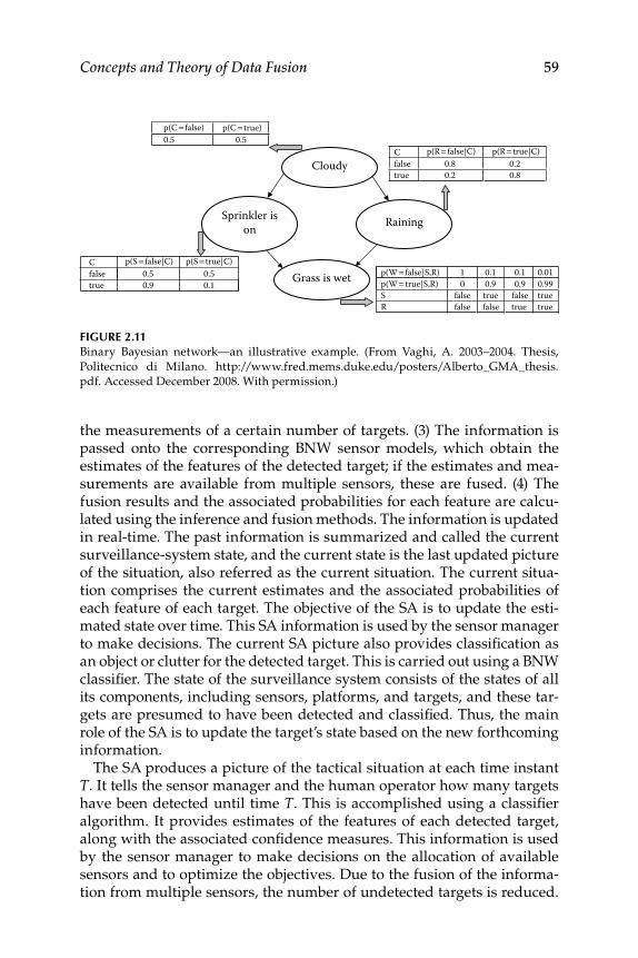
Concepts and Theory of Data Fusion 59

the measurements of a certain number of targets. (3) The information is passed onto the corresponding BNW sensor models, which obtain the estimates of the features of the detected target; if the estimates and mea-surements are available from multiple sensors, these are fused. (4) The fusion results and the associated probabilities for each feature are calcu-lated using the inference and fusion methods. The information is updated in real-time. The past information is summarized and called the current surveillance- system state, and the current state is the last updated picture of the situation, also referred as the current situation. The current situa-tion comprises the current estimates and the associated probabilities of each feature of each target. The objective of the SA is to update the esti-mated state over time. This SA information is used by the sensor manager to make decisions. The current SA picture also provides classifi cation as an object or clutter for the detected target. This is carried out using a BNW classifi er. The state of the surveillance system consists of the states of all its components, including sensors, platforms, and targets, and these tar-gets are presumed to have been detected and classifi ed. Thus, the main role of the SA is to update the target’s state based on the new forthcoming information.

The SA produces a picture of the tactical situation at each time instant T . It tells the sensor manager and the human operator how many targets have been detected until time T . This is accomplished using a classifi er algorithm. It provides estimates of the features of each detected target, along with the associated confi dence measures. This information is used by the sensor manager to make decisions on the allocation of available sensors and to optimize the objectives. Due to the fusion of the informa-tion from multiple sensors, the number of undetected targets is reduced.

FIGURE 2.11 Binary Bayesian network—an illustrative example. (From Vaghi, A. 2003–2004. Thesis,

Politecnico di Milano. http://www.fred.mems.duke.edu/posters/Alberto_GMA_thesis.

pdf. Accessed December 2008. With permission.)

p(C = false) p(C = true)0.5 0.5

C p(R = false|C) p(R = true|C) false 0.8 0.2 true 0.2 0.8

C p(S = false|C) p(S = true|C) false 0.5 0.5true 0.9 0.1

p(W = false|S,R) 1 0.1 0.1 0.01 p(W = true|S,R) 0 0.9 0.9 0.99 S false true false true R false false true true

Cloudy

Sprinkler ison Raining

Grass is wet

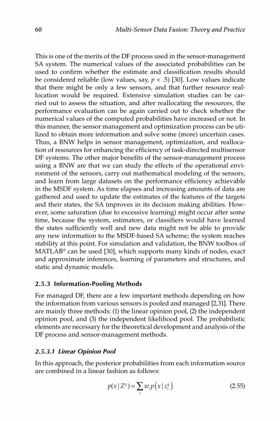
60 Multi-Sensor Data Fusion: Theory and Practice

This is one of the merits of the DF process used in the sensor-management SA system. The numerical values of the associated probabilities can be used to confi rm whether the estimate and classifi cation results should be considered reliable (low values, say, p < .5) [30]. Low values indicate that there might be only a few sensors, and that further resource real-location would be required. Extensive simulation studies can be car-ried out to assess the situation, and after reallocating the resources, the performance evaluation can be again carried out to check whether the numerical values of the computed probabilities have increased or not. In this manner, the sensor management and optimization process can be uti-lized to obtain more information and solve some (more) uncertain cases. Thus, a BNW helps in sensor management, optimization, and realloca-tion of resources for enhancing the effi ciency of task-directed multisensor DF systems. The other major benefi ts of the sensor-management process using a BNW are that we can study the effects of the operational envi-ronment of the sensors, carry out mathematical modeling of the sensors, and learn from large datasets on the performance effi ciency achievable in the MSDF system. As time elapses and increasing amounts of data are gathered and used to update the estimates of the features of the targets and their states, the SA improves in its decision making abilities. How-ever, some saturation (due to excessive learning) might occur after some time, because the system, estimators, or classifi ers would have learned the states suffi ciently well and new data might not be able to provide any new information to the MSDF-based SA scheme; the system reaches stability at this point. For simulation and validation, the BNW toolbox of MATLAB® can be used [30], which supports many kinds of nodes, exact and approximate inferences, learning of parameters and structures, and static and dynamic models.

2.5.3 Information-Pooling Methods

For managed DF, there are a few important methods depending on how the information from various sensors is pooled and managed [2,31]. There are mainly three methods: (1) the linear opinion pool, (2) the independent opinion pool, and (3) the independent likelihood pool. The probabilistic elements are necessary for the theoretical development and analysis of the DF process and sensor-management methods.

2.5.3.1 Linear Opinion Pool

In this approach, the posterior probabilities from each information source are combined in a linear fashion as follows:

p(x|Zk ) = wi

i∑ p x|zi

k( ) (2.55)

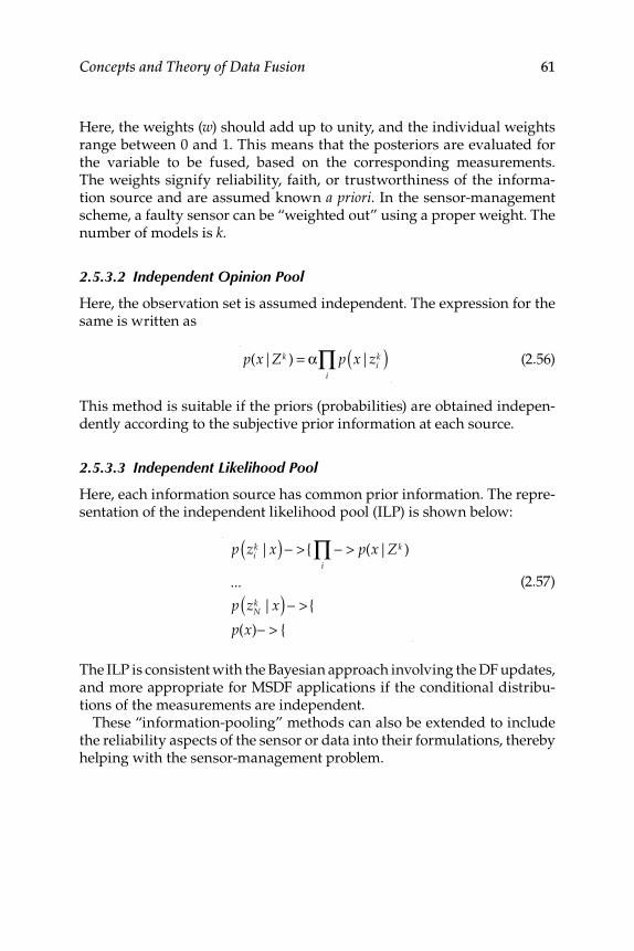
Concepts and Theory of Data Fusion 61

Here, the weights ( w ) should add up to unity, and the individual weights range between 0 and 1. This means that the posteriors are evaluated for the variable to be fused, based on the corresponding measurements. The weights signify reliability, faith, or trustworthiness of the informa-tion source and are assumed known a priori . In the sensor-management scheme, a faulty sensor can be “weighted out” using a proper weight. The number of models is k .

2.5.3.2 Independent Opinion Pool

Here, the observation set is assumed independent. The expression for the same is written as

p(x|Zk ) = α p x|zi

k( )i

∏ (2.56)

This method is suitable if the priors (probabilities) are obtained indepen-dently according to the subjective prior information at each source.

2.5.3.3 Independent Likelihood Pool

Here, each information source has common prior information. The repre-sentation of the independent likelihood pool (ILP) is shown below:

p zik |x( ) − > { − > p(x|Zk )

i∏

...

p zNk |x( ) − > {

p(x)− > {

(2.57)

The ILP is consistent with the Bayesian approach involving the DF updates, and more appropriate for MSDF applications if the conditional distribu-tions of the measurements are independent.

These “information-pooling” methods can also be extended to include the reliability aspects of the sensor or data into their formulations, thereby helping with the sensor-management problem.

63

3 Strategies and Algorithms for Target Tracking and Data Fusion

The problem of tracking moving objects—including targets, mobile robots, and other vehicles—using measurements from sensors is of con-siderable interest in many military and civil applications that use radar, sonar systems, and electro-optical tracking systems (EOTs) for tracking fl ight testing of aircrafts, such as missiles, unmanned aerial vehicles, micro- or mini-air vehicles, and rotorcrafts. It is also useful in nonmili-tary applications such as robotics, air traffi c control and management, air surveillance, and ground vehicle tracking. In practice, scenarios for tar-get tracking could include maneuvering, crossing, and splitting (meeting and separating) targets. Various algorithms are available to achieve target tracking for such scenarios. The selection of the algorithms is generally application dependent and is also based on the merits of the algorithm, complexity of the problem (data corrupted by ground clutter, noise pro-cesses, and so on), and computational burden.

Target tracking comprises estimation of the current state of a target, usually based on noisy measurements. The problem is complex even for single target tracking because of uncertainties in the target’s mathemati-cal model, especially for maneuvering targets (which need more than one model and one transition model, and so on), and process/state and measurement noises. The complexity of the tracking problem increases for multiple-targets using measurements from multiple sensors. In this chapter, we discuss several algorithms and strategies for target track-ing and associated data fusion (DF) aspects where applicable, and in Chapter 4, we present performance evaluation results for a few DF sys-tems and algorithms.

The importance of DF for tracking stems from the following consid-erations. For an aircraft observed by pulsed radar and an infrared (IR) imaging sensor, the radar provides the ability to accurately determine the aircraft’s range; however, it has only a limited ability to determine the angular direction, whereas the IR sensor can accurately deter-mine the aircraft’s angular direction, but not the range. If these two types of observations are correctly associated and fused, this will pro-vide an improved determination of range and direction than could be obtained by either of the two sensors alone. Based on an observation of

64 Multi-Sensor Data Fusion: Theory and Practice

the attributes of an object, the identity of the object can be determined and the observations of angular direction, range, and range rate may be converted to estimate the target’s position and velocity. This could be achieved using a Kalman fi lter (KF) for linear models, and an extended KF (EKF) [32,33] and derivative-free KF (DFKF) for nonlinear systems [34–37]. Then, the estimated states can be combined, as in state-vector fusion (Section 3.1). Observations of the target’s attributes, such as the radar cross section, IR spectra, and visual images, may be used to clas-sify the target and assign a label to its identity. The raw data from the sensors may be directly combined if the sensors are of the same type, that is, commensurate and similar, and measure the same physical phe-nomenon such as target range. However, in a KF the sensor data from different types of sensors (as well as the same type of sensors) can be combined appropriately via measurement models (and associated mea-surement covariance matrices) and one state vector can be estimated. In this mode, the KF is a data fuser (Section 2.2). In the case of dissimi-lar sensors (from where the data are noncommensurate and cannot be combined in a conventional way), for example, IR and acoustic data, feature and state-vector fusion may be used to combine data which are noncommensurate.

In the process of target tracking, the target track is updated by corre-lating measurements with the existing tracks or by initiating new tracks using measurements from different sensors. The process of gating and data association (DA) enables proper and accurate tracking in multisen-sor, multitarget (MSMT) scenarios [4,38,39]. Gating helps in deciding if an observation (which could include clutter, false alarms, and electronic counter measures) is a probable candidate for track maintenance or track updates. DA associates the measurements with the targets with certainty when several targets are in the same neighborhood. In practice, mea-surements from the sensors may not be true due to the effect of clutter, false alarms, interference from other targets, limited resolution capability (a spatial coverage limitation of the sensor), or if there are several targets in neighborhood.

Gating is used to screen out false signals such as clutter, whereas associ-ation algorithms are used for automatic track initiation, measurement-to-track correlation, and track-to-track correlation. In measurement-to-track correlation, the sensors’ data are associated with an existing number of tracks to determine which sensor’s data or observations belong to which target (this is the beginning of the decision level fusion; Section 7.1). Once a determination has been made that there is more than one observation for a particular target, these observations are combined at the raw level using measurement fusion, in a typical sequential estimation technique such as KF. The steps needed to implement the measurement fusion algo-rithm are described below. This is a technique for eliminating unlikely

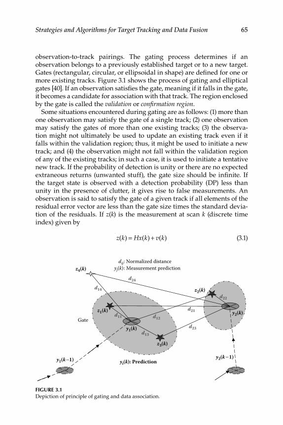
Strategies and Algorithms for Target Tracking and Data Fusion 65

observation-to-track pairings. The gating process determines if an observation belongs to a previously established target or to a new target. Gates (rectangular, circular, or ellipsoidal in shape) are defi ned for one or more existing tracks. Figure 3.1 shows the process of gating and elliptical gates [40]. If an observation satisfi es the gate, meaning if it falls in the gate, it becomes a candidate for association with that track. The region enclosed by the gate is called the validation or confi rmation region .

Some situations encountered during gating are as follows: (1) more than one observation may satisfy the gate of a single track; (2) one observation may satisfy the gates of more than one existing tracks; (3) the observa-tion might not ultimately be used to update an existing track even if it falls within the validation region; thus, it might be used to initiate a new track; and (4) the observation might not fall within the validation region of any of the existing tracks; in such a case, it is used to initiate a tentative new track. If the probability of detection is unity or there are no expected extraneous returns (unwanted stuff), the gate size should be infi nite. If the target state is observed with a detection probability (DP) less than unity in the presence of clutter, it gives rise to false measurements. An observation is said to satisfy the gate of a given track if all elements of the residual error vector are less than the gate size times the standard devia-tion of the residuals. If z ( k ) is the measurement at scan k (discrete time index) given by

z(k) = Hx(k) + v(k) (3.1)

y1(k −1)

d11

d13

d14

d12

y2(k −1)

d21

d23

d24

d22

z4(k)

z2(k)

y1(k)

y2(k)Gate

yi(k): Prediction

dij: Normalized distance yj(k): Measurement prediction

z1(k)

z3(k)

FIGURE 3.1 Depiction of principle of gating and data association.

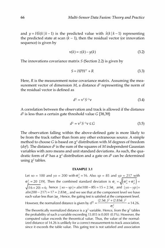
66 Multi-Sensor Data Fusion: Theory and Practice

and y = Hx(k|k − 1) is the predicted value with x(k|k − 1) representing the predicted state at scan ( k − 1), then the residual vector (or innovation sequence) is given by

ν(k) = z(k) − y(k) (3.2)

The innovations covariance matrix S (Section 2.2) is given by

S = HPHT + R (3.3)

Here, R is the measurement noise covariance matrix. Assuming the mea-surement vector of dimension M , a distance d 2 representing the norm of the residual vector is defi ned as

d2 = νTS−1ν (3.4)

A correlation between the observation and track is allowed if the distance d 2 is less than a certain gate threshold value G [38,39]:

d2 = νTS−1ν ≤ G (3.5)

The observation falling within the above-defi ned gate is more likely to be from the track rather than from any other extraneous source. A simple method to choose G is based on χ 2 distribution with M degrees of freedom ( dof ). The distance d 2 is the sum of the squares of M independent Gaussian variables with zero means and unit standard deviations. As such, the qua-dratic form of d 2 has a χ 2 distribution and a gate on d 2 can be determined using χ 2 tables.

EXAMPLE 3.1

Let xo = 100 and yo = 200 with σo2 = 16. Also xp = 85 and yp = 217 with

σp2 = 20 [39]. Then the combined standard deviation is σ r = σo

2 + σp2( ) =

(16 + 20) = 6; hence | xo − xp |= abs(100 − 85) = 15 = 2.5σ r and | yo − yp |=abs(200 − 217) = 17 = 2.83σ r , and we see that at the component level we have each value less than 3σ r

. Hence, the gating test is satisfi ed at the component level.

However, the normalized distance is given by d 2 =(2.5σ r )2 + (2.83σ r )2

σ r2

= 14.26.

The theoretically normalized distance is a χ 2 variable. Hence, from the χ 2 tables the probability of such a variable exceeding 13.815 is 0.001 (0.1%). However, the computed value exceeds the theoretical value. Thus, the value of the normal-ized distance of 14.26 is unlikely for a correct measurement-to-track association, since it exceeds the table value. This gating test is not satisfi ed and association

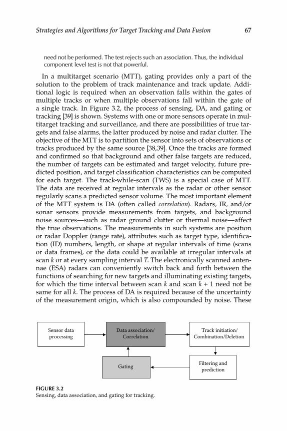
Strategies and Algorithms for Target Tracking and Data Fusion 67

need not be performed. The test rejects such an association. Thus, the individual component level test is not that powerful.

In a multitarget scenario (MTT), gating provides only a part of the solution to the problem of track maintenance and track update. Addi-tional logic is required when an observation falls within the gates of multiple tracks or when multiple observations fall within the gate of a single track. In Figure 3.2, the process of sensing, DA, and gating or tracking [39] is shown. Systems with one or more sensors operate in mul-titarget tracking and surveillance, and there are possibilities of true tar-gets and false alarms, the latter produced by noise and radar clutter. The objective of the MTT is to partition the sensor into sets of observations or tracks produced by the same source [38,39]. Once the tracks are formed and confi rmed so that background and other false targets are reduced, the number of targets can be estimated and target velocity, future pre-dicted position, and target classifi cation characteristics can be computed for each target. The track-while-scan (TWS) is a special case of MTT. The data are received at regular intervals as the radar or other sensor regularly scans a predicted sensor volume. The most important element of the MTT system is DA (often called correlation ). Radars, IR, and/or sonar sensors provide measurements from targets, and background noise sources—such as radar ground clutter or thermal noise—affect the true observations. The measurements in such systems are position or radar Doppler (range rate), attributes such as target type, identifi ca-tion (ID) numbers, length, or shape at regular intervals of time (scans or data frames), or the data could be available at irregular intervals at scan k or at every sampling interval T . The electronically scanned anten-nae (ESA) radars can conveniently switch back and forth between the functions of searching for new targets and illuminating existing targets, for which the time interval between scan k and scan k + 1 need not be same for all k . The process of DA is required because of the uncertainty of the measurement origin, which is also compounded by noise. These

FIGURE 3.2 Sensing, data association, and gating for tracking.

Track initiation/Combination/Deletion

Sensor dataprocessing

Data association/Correlation

Gating Filtering andprediction

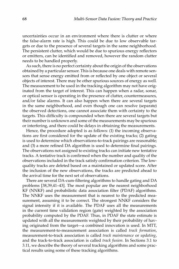
68 Multi-Sensor Data Fusion: Theory and Practice

uncertainties occur in an environment where there is clutter or where the false-alarm rate is high. This could be due to low observable tar-gets or due to the presence of several targets in the same neighborhood. The persistent clutter, which would be due to spurious energy refl ectors or emitters, can be identifi ed and removed, however the random clutter needs to be handled properly.

As such, there is no perfect certainty about the origin of the observations obtained by a particular sensor. This is because one deals with remote sen-sors that sense energy emitted from or refl ected by one object or several objects of interest. There may be other spurious sources of energy as well. The measurement to be used in the tracking algorithm may not have orig-inated from the target of interest. This can happen when a radar, sonar, or optical sensor is operating in the presence of clutter, countermeasures, and/or false alarms. It can also happen when there are several targets in the same neighborhood, and even though one can resolve (separate) the observed detections, one cannot associate them with certainty to the targets. This diffi culty is compounded when there are several targets but their number is unknown and some of the measurements may be spurious or interfering, and there could be delays in obtaining the measurements.

Hence, the procedure adopted is as follows: (1) the incoming observa-tions are fi rst considered for the update of the existing tracks; (2) gating is used to determine which observations-to-track pairings are reasonable; and (3) a more refi ned DA algorithm is used to determine fi nal pairings. The observations not assigned to existing tracks can initiate new tentative tracks. A tentative track is confi rmed when the number and quality of the observations included in the track satisfy confi rmation criterion. The low-quality tracks are deleted based on a maintained or updated score. After the inclusion of the new observations, the tracks are predicted ahead to the arrival time for the next set of observations.

There are several DA-cum-fi ltering algorithms to handle gating and DA problems [38,39,41–43]. The most popular are the nearest neighborhood KF (NNKF) and probabilistic data association fi lter (PDAF) algorithms. The NNKF uses the measurement that is nearest to the predicted mea-surement, assuming it to be correct. The strongest NNKF considers the signal intensity if it is available. The PDAF uses all the measurements in the current time validation region (gate) weighted by the association probability computed by the PDAF. Thus, in PDAF the state estimate is updated with all the measurements weighted by their probability of hav-ing originated from the target—a combined innovation is used. In MTT, the measurement-to-measurement association is called track formation , measurement-to-track association is called track maintenance or updating , and the track-to-track association is called track fusion . In Sections 3.1 to 3.11, we describe the theory of several tracking algorithms and some prac-tical results using some of these tracking algorithms.

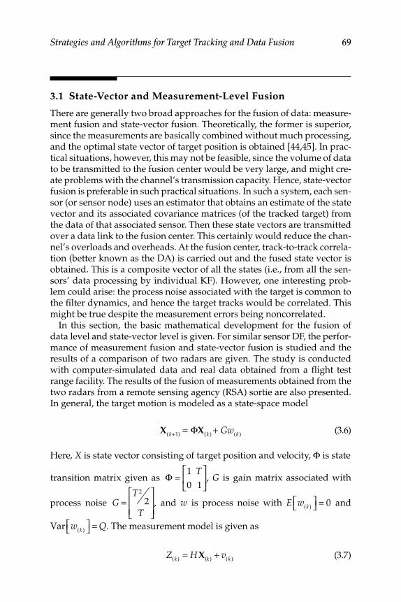
Strategies and Algorithms for Target Tracking and Data Fusion 69

3.1 State-Vector and Measurement-Level Fusion

There are generally two broad approaches for the fusion of data: measure-ment fusion and state-vector fusion. Theoretically, the former is superior, since the measurements are basically combined without much processing, and the optimal state vector of target position is obtained [44,45]. In prac-tical situations, however, this may not be feasible, since the volume of data to be transmitted to the fusion center would be very large, and might cre-ate problems with the channel’s transmission capacity. Hence, state-vector fusion is preferable in such practical situations. In such a system, each sen-sor (or sensor node) uses an estimator that obtains an estimate of the state vector and its associated covariance matrices (of the tracked target) from the data of that associated sensor. Then these state vectors are transmitted over a data link to the fusion center. This certainly would reduce the chan-nel’s overloads and overheads. At the fusion center, track-to-track correla-tion (better known as the DA) is carried out and the fused state vector is obtained. This is a composite vector of all the states (i.e., from all the sen-sors’ data processing by individual KF). However, one interesting prob-lem could arise: the process noise associated with the target is common to the fi lter dynamics, and hence the target tracks would be correlated. This might be true despite the measurement errors being noncorrelated.

In this section, the basic mathematical development for the fusion of data level and state-vector level is given. For similar sensor DF, the perfor-mance of measurement fusion and state-vector fusion is studied and the results of a comparison of two radars are given. The study is conducted with computer-simulated data and real data obtained from a fl ight test range facility. The results of the fusion of measurements obtained from the two radars from a remote sensing agency (RSA) sortie are also presented. In general, the target motion is modeled as a state-space model

X

(k+1)= ΦX

(k )+ Gw

(k ) (3.6)

Here, X is state vector consisting of target position and velocity, Φ is state

transition matrix given as

Φ =

1 T

0 1

⎡

⎣⎢

⎤

⎦⎥, G is gain matrix associated with

process noise G =T 2

2

T

⎡

⎣⎢⎢

⎤

⎦⎥⎥, and w is process noise with E w

(k )⎡⎣ ⎤⎦ = 0 and

Var w(k )

⎡⎣ ⎤⎦ = Q. The measurement model is given as

Z(k )

= HX(k )

+ v(k ) (3.7)

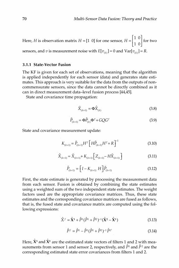
70 Multi-Sensor Data Fusion: Theory and Practice

Here, H is observation matrix H = [1 0] for one sensor, H =1 0

1 0

⎡

⎣⎢

⎤

⎦⎥ for two

sensors, and v is measurement noise with E[v(k )

] = 0 and Var[v(k )

] = R.

3.1.1 State-Vector Fusion

The KF is given for each set of observations, meaning that the algorithm is applied independently for each sensor (data) and generates state esti-mates. This approach is very suitable for the data from the outputs of non-commensurate sensors, since the data cannot be directly combined as it can in direct measurement data–level fusion process [44,45].

State and covariance time propagation:

%X

(k+1)= ΦX

(k ) (3.8)

%P(k+1)

= ΦP(k )

ΦT + GQGT (3.9)

State and covariance measurement update:

K

(k+1)= %P

(k+1)HT H %P

(k+1)HT + R⎡⎣ ⎤⎦

−1

(3.10)

X

(k+1)= %X

(k+1)+ K

(k+1)Z

(k+1)− H %X

(k+1)⎡⎣ ⎤⎦ (3.11)

P

(k+1)= I − K

(k+1) H⎡⎣ ⎤⎦

%P(k+1) (3.12)

First, the state estimate is generated by processing the measurement data from each sensor. Fusion is obtained by combining the state estimates using a weighted sum of the two independent state estimates. The weight factors used are the appropriate covariance matrices. Thus, these state estimates and the corresponding covariance matrices are fused as follows, that is, the fused state and covariance matrix are computed using the fol-lowing expressions:

X

f = X1 + P1(P1 + P2 )−1(X2 − X1 ) (3.13)

P

f = P1 − P1(P1 + P2 )−1 P1T (3.14)

Here, X1 and X2 are the estimated state vectors of fi lters 1 and 2 with mea-

surements from sensor 1 and sensor 2, respectively, and P1 and P 2 are the corresponding estimated state error covariances from fi lters 1 and 2.

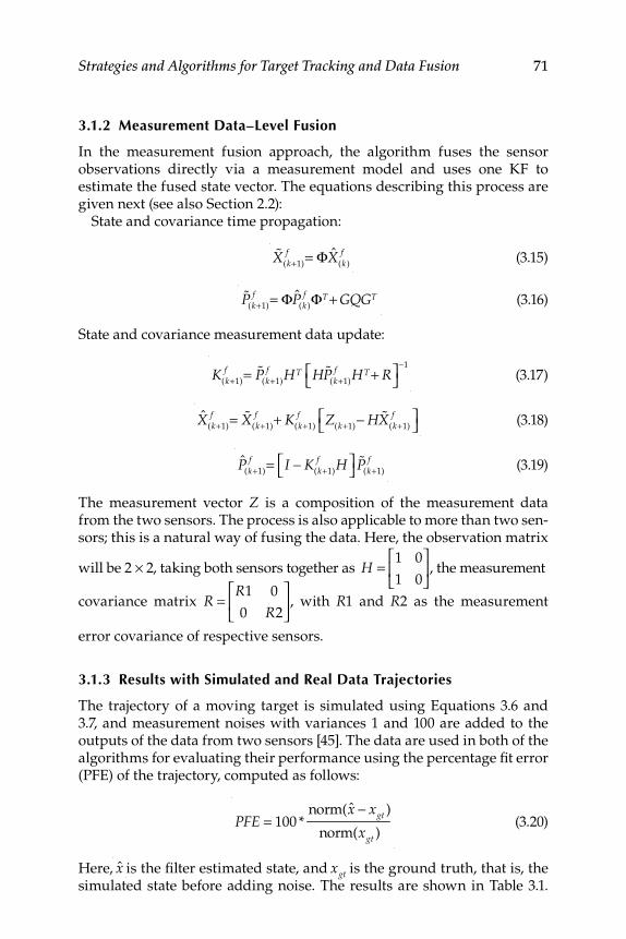
Strategies and Algorithms for Target Tracking and Data Fusion 71

3.1.2 Measurement Data–Level Fusion

In the measurement fusion approach, the algorithm fuses the sensor observations directly via a measurement model and uses one KF to estimate the fused state vector. The equations describing this process are given next (see also Section 2.2):

State and covariance time propagation:

%X

(k+1)

f = ΦX(k )

f (3.15)

%P(k+1)

f = ΦP(k )

f ΦT + GQGT (3.16)

State and covariance measurement data update:

K

(k+1)

f = %P(k+1)

f HT H %P(k+1)

f HT + R⎡⎣

⎤⎦

−1

(3.17)

X

(k+1)

f = %X(k+1)

f + K(k+1)

f Z(k+1)

− H %X(k+1)

f⎡⎣

⎤⎦ (3.18)

P

(k+1)

f = I − K(k+1)

f H⎡⎣

⎤⎦

%P(k+1)

f (3.19)

The measurement vector Z is a composition of the measurement data from the two sensors. The process is also applicable to more than two sen-sors; this is a natural way of fusing the data. Here, the observation matrix

will be 2 × 2, taking both sensors together as

H =

1 0

1 0

⎡

⎣⎢

⎤

⎦⎥, the measurement

covariance matrix R =R1 0

0 R2

⎡

⎣⎢

⎤

⎦⎥, with R 1 and R 2 as the measurement

error covariance of respective sensors.

3.1.3 Results with Simulated and Real Data Trajectories

The trajectory of a moving target is simulated using Equations 3.6 and 3.7, and measurement noises with variances 1 and 100 are added to the outputs of the data from two sensors [45]. The data are used in both of the algorithms for evaluating their performance using the percentage fi t error (PFE) of the trajectory, computed as follows:

PFE = 100 *norm(x − xgt )

norm(xgt ) (3.20)

Here, x is the fi lter estimated state, and xgt is the ground truth, that is, the simulated state before adding noise. The results are shown in Table 3.1.

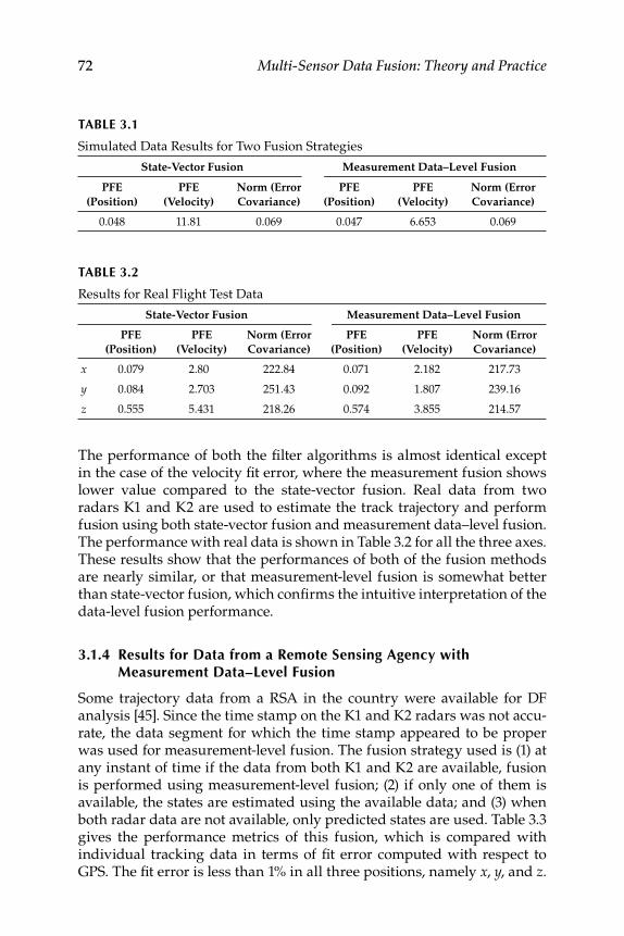
72 Multi-Sensor Data Fusion: Theory and Practice

The performance of both the fi lter algorithms is almost identical except in the case of the velocity fi t error, where the measurement fusion shows lower value compared to the state-vector fusion. Real data from two radars K1 and K2 are used to estimate the track trajectory and perform fusion using both state-vector fusion and measurement data–level fusion. The performance with real data is shown in Table 3.2 for all the three axes. These results show that the performances of both of the fusion methods are nearly similar, or that measurement-level fusion is somewhat better than state-vector fusion, which confi rms the intuitive interpretation of the data-level fusion performance.

3.1.4 Results for Data from a Remote Sensing Agency with Measurement Data–Level Fusion

Some trajectory data from a RSA in the country were available for DF analysis [45]. Since the time stamp on the K1 and K2 radars was not accu-rate, the data segment for which the time stamp appeared to be proper was used for measurement-level fusion. The fusion strategy used is (1) at any instant of time if the data from both K1 and K2 are available, fusion is performed using measurement-level fusion; (2) if only one of them is available, the states are estimated using the available data; and (3) when both radar data are not available, only predicted states are used. Table 3.3 gives the performance metrics of this fusion, which is compared with individual tracking data in terms of fi t error computed with respect to GPS. The fi t error is less than 1% in all three positions, namely x , y , and z .

TABLE 3.1

Simulated Data Results for Two Fusion Strategies

State-Vector Fusion Measurement Data–Level Fusion

PFE

(Position)

PFE

(Velocity)

Norm (Error

Covariance)

PFE

(Position)

PFE

(Velocity)

Norm (Error

Covariance)

0.048 11.81 0.069 0.047 6.653 0.069

TABLE 3.2

Results for Real Flight Test Data

State-Vector Fusion Measurement Data–Level Fusion

PFE

(Position)

PFE

(Velocity)

Norm (Error

Covariance)

PFE

(Position)

PFE

(Velocity)

Norm (Error

Covariance)

x 0.079 2.80 222.84 0.071 2.182 217.73

y 0.084 2.703 251.43 0.092 1.807 239.16

z 0.555 5.431 218.26 0.574 3.855 214.57

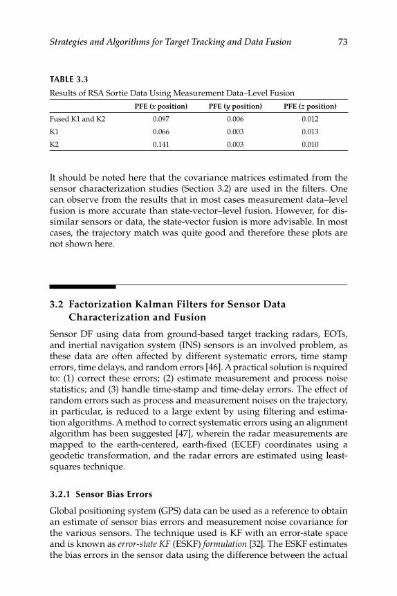
Strategies and Algorithms for Target Tracking and Data Fusion 73

It should be noted here that the covariance matrices estimated from the sensor characterization studies (Section 3.2) are used in the fi lters. One can observe from the results that in most cases measurement data–level fusion is more accurate than state-vector–level fusion. However, for dis-similar sensors or data, the state-vector fusion is more advisable. In most cases, the trajectory match was quite good and therefore these plots are not shown here.

3.2 Factorization Kalman Filters for Sensor Data

Characterization and Fusion

Sensor DF using data from ground-based target tracking radars, EOTs, and inertial navigation system (INS) sensors is an involved problem, as these data are often affected by different systematic errors, time stamp errors, time delays, and random errors [46]. A practical solution is required to: (1) correct these errors; (2) estimate measurement and process noise statistics; and (3) handle time-stamp and time-delay errors. The effect of random errors such as process and measurement noises on the trajectory, in particular, is reduced to a large extent by using fi ltering and estima-tion algorithms. A method to correct systematic errors using an alignment algorithm has been suggested [47], wherein the radar measurements are mapped to the earth-centered, earth-fi xed (ECEF) coordinates using a geodetic transformation, and the radar errors are estimated using least-squares technique.

3.2.1 Sensor Bias Errors

Global positioning system (GPS) data can be used as a reference to obtain an estimate of sensor bias errors and measurement noise covariance for the various sensors. The technique used is KF with an error-state space and is known as error-state KF (ESKF) formulation [32]. The ESKF estimates the bias errors in the sensor data using the difference between the actual

TABLE 3.3

Results of RSA Sortie Data Using Measurement Data–Level Fusion

PFE (x position) PFE (y position) PFE (z position)

Fused K1 and K2 0.097 0.006 0.012

K1 0.066 0.003 0.013

K2 0.141 0.003 0.010

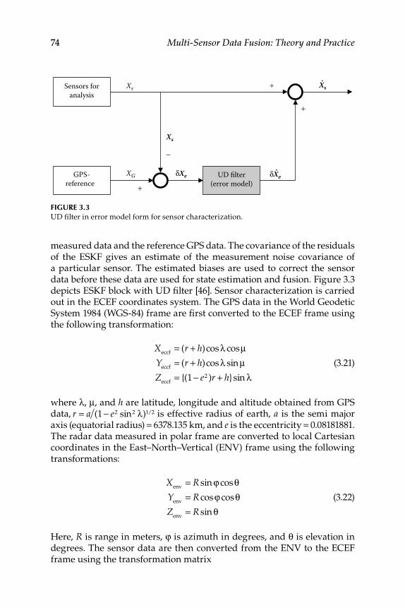
74 Multi-Sensor Data Fusion: Theory and Practice

measured data and the reference GPS data. The covariance of the residuals of the ESKF gives an estimate of the measurement noise covariance of a particular sensor. The estimated biases are used to correct the sensor data before these data are used for state estimation and fusion. Figure 3.3 depicts ESKF block with UD fi lter [46]. Sensor characterization is carried out in the ECEF coordinates system. The GPS data in the World Geodetic System 1984 (WGS-84) frame are fi rst converted to the ECEF frame using the following transformation:

Xeccf

= (r + h)cosλ cosμY

eccf= (r + h)cosλ sin μ

Zeccf

= {(1 − e2 )r + h} sin λ (3.21)

where λ, μ, and h are latitude, longitude and altitude obtained from GPS data, r = a (1 − e2 sin2 λ)1/2 is effective radius of earth, a is the semi major axis (equatorial radius) = 6378.135 km, and e is the eccentricity = 0.08181881. The radar data measured in polar frame are converted to local Cartesian coordinates in the East–North–Vertical (ENV) frame using the following transformations:

Xenv

= R sin ϕ cosθY

env= R cosϕ cosθ

Zenv

= R sin θ (3.22)

Here, R is range in meters, ϕ is azimuth in degrees, and θ is elevation in degrees. The sensor data are then converted from the ENV to the ECEF frame using the transformation matrix

FIGURE 3.3 UD fi lter in error model form for sensor characterization.

Sensors foranalysis

GPS-reference

UD filter(error model)

Xs

Xs

XG

+

+

+

−

ˆδXeδXe

Xs

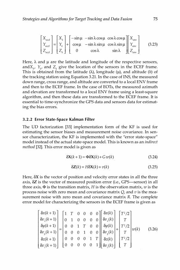
Strategies and Algorithms for Target Tracking and Data Fusion 75

Xeccf

Yeccf

Zeccf

⎡

⎣

⎢⎢⎢

⎤

⎦

⎥⎥⎥

=Xk

Yk

Zk

⎡

⎣

⎢⎢⎢

⎤

⎦

⎥⎥⎥

+− sin μ − sin λ cosμ cos λ cosμcosμ − sin λ sin μ cos λ sin μ

0 cosλ sin λ

⎡

⎣

⎢⎢⎢

⎤

⎦

⎥⎥⎥

Xenv

Yenv

Zenv

⎡

⎣

⎢⎢⎢

⎤

⎦

⎥⎥⎥

(3.23)

Here, λ and μ are the latitude and longitude of the respective sensors, andXk, Yk, and Zk give the location of the sensors in the ECEF frame. This is obtained from the latitude ( λ ), longitude ( μ ), and altitude ( h ) of the tracking station using Equation 3.21. In the case of INS, the measured down range, cross range, and altitude are converted to a local ENV frame and then to the ECEF frame. In the case of EOTs, the measured azimuth and elevation are transformed to a local ENV frame using a least-square algorithm, and then these data are transformed to the ECEF frame. It is essential to time-synchronize the GPS data and sensors data for estimat-ing the bias errors.

3.2.2 Error State-Space Kalman Filter

The UD factorization [33] implementation form of the KF is used for estimating the sensor biases and measurement noise covariance. In sen-sor characterization, the KF is implemented with the “error state-space” model instead of the actual state-space model. This is known as an indirect method [32]. This error model is given as

δX(k + 1) = ΦδX(k) + Gw(k) (3.24)

δZ(k) = HδX(k) + v(k) (3.25)

Here, δX is the vector of position and velocity error states in all the three axis, δZ is the vector of measured position error (i.e., GPS—sensor) in all three axis, Φ is the transition matrix, H is the observation matrix, w is the process noise with zero mean and covariance matrix Q , and v is the mea-surement noise with zero mean and covariance matrix R . The complete error model for characterizing the sensors in the ECEF frame is given as

δx(k + 1)

δvx(k + 1)

δy(k + 1)

δvy(k + 1)

δz(k + 1)

δvz(k + 1)

⎡

⎣

⎢⎢⎢⎢⎢⎢⎢⎢

⎤

⎦

⎥⎥⎥⎥⎥⎥⎥⎥

=

1 T

0 1

0 0

0 0

0 0

0 0

0 0

0 0

1 T

0 1

0 0

0 0

0 0

0 0

0 0

0 0

1 T

0 1

⎡

⎣

⎢⎢⎢⎢⎢⎢⎢⎢

⎤

⎦

⎥⎥⎥⎥⎥⎥⎥⎥

δx(k)

δvx(k)

δy(k)

δvy(k)

δz(k)

δvz(k)

⎡

⎣

⎢⎢⎢⎢⎢⎢⎢⎢

⎤

⎦

⎥⎥⎥⎥⎥⎥⎥⎥

+

T 2/2

T

T 2/2

T

T 2/2

T

⎡

⎣

⎢⎢⎢⎢⎢⎢⎢⎢

⎤

⎦

⎥⎥⎥⎥⎥⎥⎥⎥

w(k) (3.26)

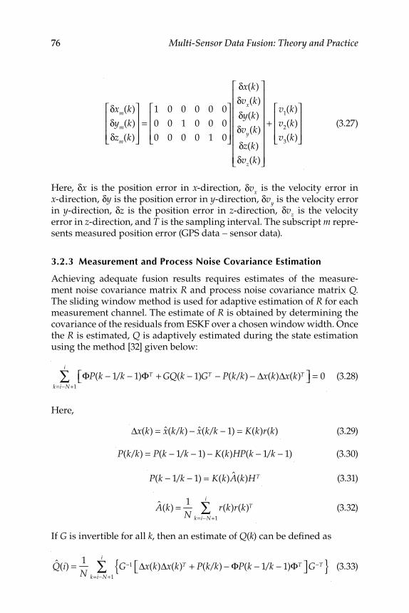
76 Multi-Sensor Data Fusion: Theory and Practice

δxm(k)

δym(k)

δzm(k)

⎡

⎣

⎢⎢⎢

⎤

⎦

⎥⎥⎥

=1 0 0 0 0 0

0 0 1 0 0 0

0 0 0 0 1 0

⎡

⎣

⎢⎢⎢

⎤

⎦

⎥⎥⎥

δx(k)

δvx(k)

δy(k)

δvy(k)

δz(k)

δvz(k)

⎡

⎣

⎢⎢⎢⎢⎢⎢⎢⎢

⎤

⎦

⎥⎥⎥⎥⎥⎥⎥⎥

+v1

(k)

v2(k)

v3(k)

⎡

⎣

⎢⎢⎢

⎤

⎦

⎥⎥⎥

(3.27)

Here, δx is the position error in x -direction, δvx is the velocity error in x -direction, δy is the position error in y -direction, δvy is the velocity error in y -direction, δz is the position error in z -direction, δvz is the velocity error in z -direction, and T is the sampling interval. The subscript m repre-sents measured position error (GPS data − sensor data).

3.2.3 Measurement and Process Noise Covariance Estimation

Achieving adequate fusion results requires estimates of the measure-ment noise covariance matrix R and process noise covariance matrix Q . The sliding window method is used for adaptive estimation of R for each measurement channel. The estimate of R is obtained by determining the covariance of the residuals from ESKF over a chosen window width. Once the R is estimated, Q is adaptively estimated during the state estimation using the method [32] given below:

ΦP(k − 1/k − 1)ΦT + GQ(k − 1)GT − P(k/k) − Δx(k)Δx(k)T⎡⎣ ⎤⎦

k=i−N+1

i

∑ = 0 (3.28)

Here,

Δx(k) = x(k/k) − x(k/k − 1) = K(k)r(k) (3.29)

P(k/k) = P(k − 1/k − 1) − K(k)HP(k − 1/k − 1) (3.30)

P(k − 1/k − 1) = K(k)A(k)HT (3.31)

A(k) = 1

Nr(k)r(k)T

k=i−N+1

i

∑ (3.32)

If G is invertible for all k , then an estimate of Q ( k ) can be defi ned as

Q(i) = 1

NG−1 Δx(k)Δx(k)T + P(k/k) − ΦP(k − 1/k − 1)ΦT⎡⎣ ⎤⎦ G−T{ }

k=i−N+1

i

∑ (3.33)

Strategies and Algorithms for Target Tracking and Data Fusion 77

If G is not invertible, then pseudo-inverse is used, computed as

G# = [GTG]−1GT (3.34)

3.2.4 Time Stamp and Time Delay Errors

The fusion of data from two or more sensors requires that the mea-surements are available at the same instant of time and that the data are received with an accurate time stamp, corresponding to the time at which the data were sensed or acquired by the sensor or data acquisition system. This is not always the case—the data could come with erroneous time stamps either at the transmitting end or at the receiving end. There could be drifts in the time recorded on any channel. This time drift could either be of a constant value on any channel or could be different (ran-dom) at each instant of time. Some practical aspects on this issue are as follows: (1) the fi rst few samples of data can be used to ascertain constant time drift on any channel and the subsequent time stamps can be cor-rected by the computed time drift; (2) to handle random time drift, at any instant of time, any data coming within one-half of the sampling time on that channel can be treated as if it has arrived at that instant for purpose of fusion; and (3) for state-vector fusion, it is expected that the output of the fi lter is available at every T seconds (reference sampling time). This is achieved by using the data arriving at each instant for updating the states of the fi lter and propagating the estimated states to the nearest T, so that it is available for fusion there. This method of synchronizing the state vectors for fusion presupposes that the sampling time require-ments are appropriately chosen to suit the dynamics of the target being tracked.

3.2.5 Multisensor Data Fusion Scheme

Figure 3.4 shows a block diagram of the multisensor DF (MSDF) scheme [46]. The fi rst step is time synchronization of various sensors’ data. For this step, the data arrival on each of the tracking sensor data (including GPS) is checked and a reference time signal is initiated using the time stamp on the sensor data that arrives fi rst. This time signal is incre-mented at a uniform rate of T seconds. At each step, the sensor time stamp on each of the input data channels is compared with the reference time and appropriate action is initiated using “decision logic” based on the time delay error handling procedure mentioned above. Each data set is appropriately transformed to the ECEF frame using the standard trans-formation equations mentioned earlier. With a GPS signal as a reference, all the sensors’ data are characterized by estimating bias and measure-ment and process noise covariance as mentioned earlier. These data are

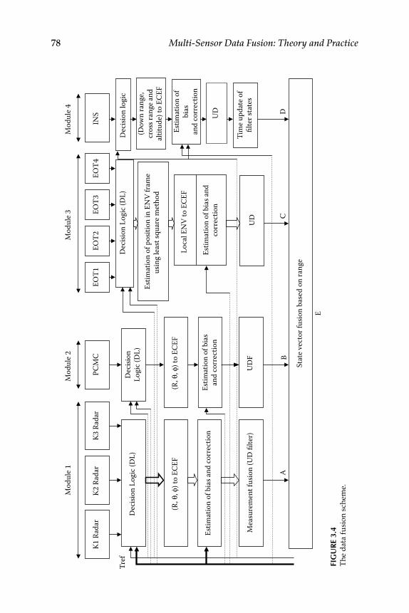
78 Multi-Sensor Data Fusion: Theory and Practice

K1 R

adar

K2 R

adar

K3

Rad

arEO

T1EO

T4EO

T3EO

T2IN

S

Dec

ision

Log

ic (D

L)

Tref

Estim

atio

n of

bias

and

corr

ectio

n

Mea

sure

men

t fus

ion

(UD

filte

r)

Stat

e vec

tor f

usio

n ba

sed

on ra

nge

Decis

ion

Logi

c (DL

)

(R, θ

, φ) t

o EC

EF

(R, θ

, φ) t

o EC

EF

Estim

atio

n of

bias

and

corr

ectio

n

UDF

Dec

ision

Log

ic (D

L)

Estim

atio

n of

pos

ition

in E

NV

fram

eus

ing l

east

squa

re m

etho

d

Estim

atio

n of

bias

and

corr

ectio

n

UD

Estim

atio

n of

bias

and

corr

ectio

n

(Dow

n ra

nge,

cros

s ran

ge an

dalt

itude

) to

ECEF

Mod

ule 1

Mod

ule 3

M

odul

e 4

Loca

l EN

V to

ECE

F

UD

Tim

e upd

ate o

ffil

ter s

tate

s

Dec

ision

logi

c

AB

CD

E

PCM

C

Mod

ule 2

FIG

UR

E 3.

4 T

he

dat

a f

usi

on

sch

eme.

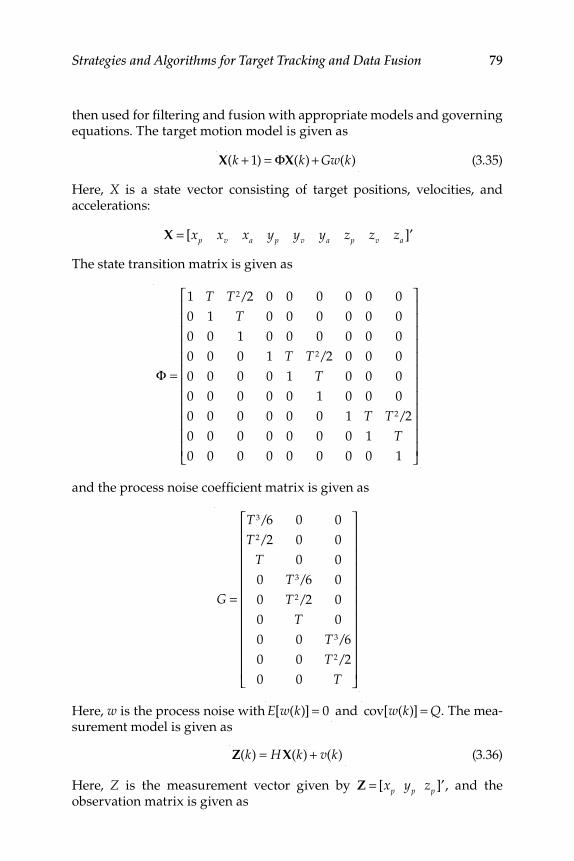
Strategies and Algorithms for Target Tracking and Data Fusion 79

then used for fi ltering and fusion with appropriate models and governing equations. The target motion model is given as

X(k + 1) = ΦX(k) + Gw(k) (3.35)

Here, X is a state vector consisting of target positions, velocities, and accelerations:

X = [xp xv xa yp yv ya zp zv za ′]

The state transition matrix is given as

Φ =

1 T T 2/2 0 0 0 0 0 0

0 1 T 0 0 0 0 0 0

0 0 1 0 0 0 0 0 0

0 0 0 1 T T 2/2 0 0 0

0 0 0 0 1 T 0 0 0

0 0 0 0 0 1 0 0 0

0 0 0 0 0 0 1 T T 2/2

0 0 0 0 0 0 0 1 T

0 0 0 0 0 0 0 0 1

⎡

⎣

⎢⎢⎢⎢⎢⎢⎢⎢⎢⎢⎢⎢

⎤

⎦

⎥⎥⎥⎥⎥⎥⎥⎥⎥⎥⎥⎥

and the process noise coeffi cient matrix is given as

G =

T 3/6 0 0

T 2/2 0 0

T 0 0

0 T 3/6 0

0 T 2/2 0

0 T 0

0 0 T 3/6

0 0 T 2/2

0 0 T

⎡

⎣

⎢⎢⎢⎢⎢⎢⎢⎢⎢⎢⎢⎢

⎤

⎦

⎥⎥⎥⎥⎥⎥⎥⎥⎥⎥⎥⎥

Here, w is the process noise with E[w(k)] = 0 and

cov[w(k)] = Q. The mea-surement model is given as

Z(k) = HX(k) + v(k) (3.36)

Here, Z is the measurement vector given by Z = [xp yp zp ′] , and the observation matrix is given as

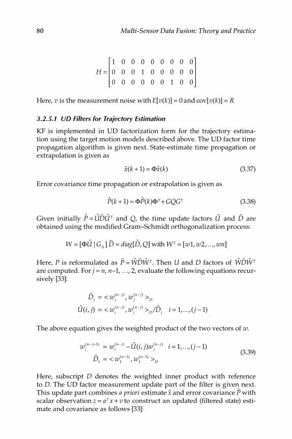
80 Multi-Sensor Data Fusion: Theory and Practice

H =1 0 0 0 0 0 0 0 0

0 0 0 1 0 0 0 0 0

0 0 0 0 0 0 1 0 0

⎡

⎣

⎢⎢⎢

⎤

⎦

⎥⎥⎥

Here, v is the measurement noise with E[v(k)] = 0 and

cov[v(k)] = R

3.2.5.1 UD Filters for Trajectory Estimation

KF is implemented in UD factorization form for the trajectory estima-tion using the target motion models described above. The UD factor time propagation algorithm is given next. State-estimate time propagation or extrapolation is given as

%x(k + 1) = Φx(k) (3.37)

Error covariance time propagation or extrapolation is given as

%P(k + 1) = ΦP(k)ΦT + GQGT (3.38)

Given initially P = UDUT and Q , the time update factors %U and %D are obtained using the modifi ed Gram–Schmidt orthogonalization process:

W = [ΦU|GA ] D = diag[D,Q] with WT = [w1, w2, ..., wn]

Here, P is reformulated as %P = %W %D %WT. Then U and D factors of %W %D %WT are computed. For j = n , n− 1, …, 2, evaluate the following equations recur-sively [33]:

%Dj = < wj(n− j) , wj

(n− j) >D

%U(i, j) = < wi(n− j) , wj

(n− j) >D/ %Dj i = 1,..., ( j − 1)

The above equation gives the weighted product of the two vectors of w .

wi(n− j+1) = wi

(n− j) − %U(i, j)wj(n− j) i = 1,..., ( j − 1)

%D1

= < w1

(n−1) , w1

(n−1) >D

(3.39)

Here, subscript D denotes the weighted inner product with reference to D . The UD factor measurement update part of the fi lter is given next. This update part combines a priori estimate %x and error covariance %P with scalar observation z = aT x + v to construct an updated (fi ltered state) esti-mate and covariance as follows [33]:

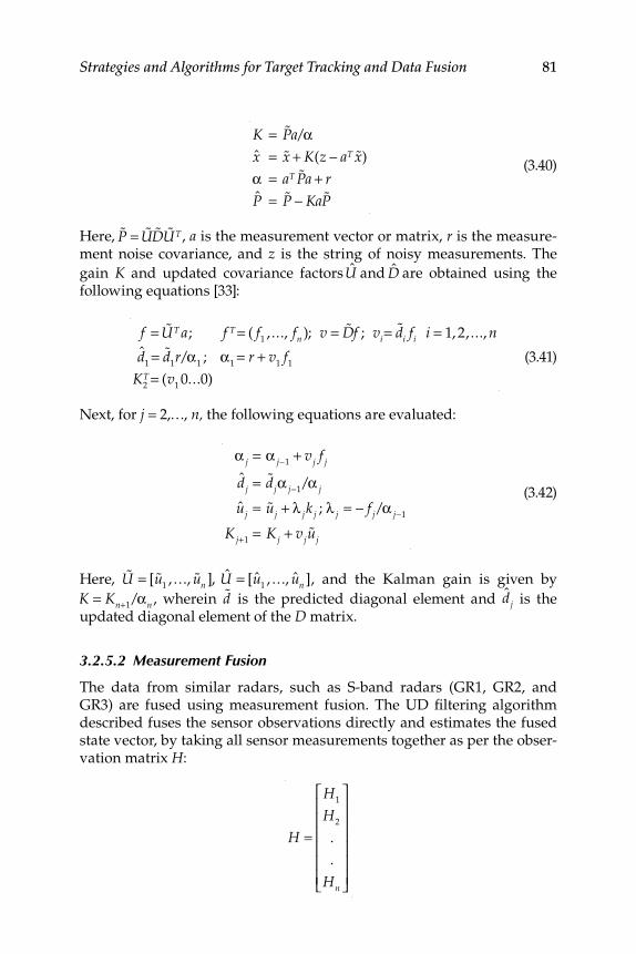
Strategies and Algorithms for Target Tracking and Data Fusion 81

K = %Pa/αx = %x + K(z − aT %x)

α = aT %Pa + r

P = %P − Ka %P

(3.40)

Here, %P = %U %D %UT, a is the measurement vector or matrix, r is the measure-ment noise covariance, and z is the string of noisy measurements. The

gain K and updated covariance factorsU and D are obtained using the following equations [33]:

f = %UT a; f T = ( f1, ..., fn ); v = %Df ; vi= %di fi i = 1, 2, ..., n

d1= %d

1r/α

1; α

1= r + v

1f1

K2T = (v

10...0)

(3.41)

Next, for j = 2,…, n, the following equations are evaluated:

α j = α j−1+ vj f j

dj = %djα j−1/α j

uj = %uj + λ jk j ; λ j = − f j/α j−1

Kj+1= Kj + vj

%uj

(3.42)

Here, %U = [ %u1, ..., %un ], U = [u

1, ..., un ], and the Kalman gain is given by

K = Kn+1/αn , wherein %d is the predicted diagonal element and dj is the

updated diagonal element of the D matrix.

3.2.5.2 Measurement Fusion

The data from similar radars, such as S-band radars (GR1, GR2, and GR3) are fused using measurement fusion. The UD fi ltering algorithm described fuses the sensor observations directly and estimates the fused state vector, by taking all sensor measurements together as per the obser-vation matrix H:

H =

H1

H2

.

.

Hn

⎡

⎣

⎢⎢⎢⎢⎢⎢

⎤

⎦

⎥⎥⎥⎥⎥⎥

82 Multi-Sensor Data Fusion: Theory and Practice

Here, H 1 , H 2 , …, H n are observation matrices of n individual sensors. The measurement covariance matrix is given as

R =

R1

0 0 0 0

0 R2

0 0 0

0 0 . 0 0

0 0 0 . 0

0 0 0 0 Rn

⎡

⎣

⎢⎢⎢⎢⎢⎢

⎤

⎦

⎥⎥⎥⎥⎥⎥

Here, R 1 , R 2 , …, R n are the measurement error covariance values of respec-tive sensors.

3.2.5.3 State-Vector Fusion

Fusion is performed as follows:

X

f = X1 + P1(P1 + P2 )−1(X 2 − X1) (3.43)

P

f = P1 − P1(P1 + P2 )−1 P1T (3.44)

Here, X1 and X 2 are the state vectors of estimated trajectories 1 and 2, and

P1 and P 2 are the state error covariance matrices of estimated trajectories 1 and 2. In this method, only two trajectories are fused at a time.

3.2.5.4 Fusion Philosophy

All the tracking sensors are grouped into four major groups (Figure 3.4) [46] based on the type, sensitivity, and accuracy of the sensors. The four major groups are as follows:

1. Module 1: The tracking data from the three radars, after coordinate transformation and characterization, are fused to get single trajec-tory data (trajectory A) by direct measurement fusion using UD-KF.

2. Module 2: The tracking data from the precision coherent mono-pulse C-band (PCMC) radar, after coordinate transformation and characterization, are fi ltered (trajectory B) using UD-KF.

3. Module 3: The tracking data (azimuth and elevation) from EOTs are fi rst transformed to local ENV frame using least-square method and then transformed to ECEF. These data are then fi l-tered (trajectory C) using UD-KF.

4. Module 4: The tracking data from the onboard inertial naviga-tion system (INS) are telemetered at a sampling interval of 72 ms.

Strategies and Algorithms for Target Tracking and Data Fusion 83

These data (down range, cross range and altitude) are transformed to ECEF, characterized, and fi ltered (trajectory D). The data are then time propagated in ECEF coordinates using target dynamic model to time synchronize with other track data. These trajecto-ries (trajectory A, trajectory B, trajectory C, and trajectory D) are then fused using state-vector fusion.

A hierarchical order, based on the accuracies of sensors, is chosen for gen-erating the fi nal trajectory estimates. EOT sensors are accurate up to a maximum range of 40 km. The following criteria are used to decide the priority for fusion:

1. If estimated range is less than 40 km, trajectory C is fused with trajectory A. The resultant trajectory is fused with trajectory B and fi nally this resultant trajectory is fused with trajectory D (INS).

2. If the estimated range is greater than 40 km, trajectory A is fused with trajectory B and the resultant trajectory is fi nally fused with trajectory D. That is, if the estimated range is less than 40 km, tra-jectory C is used for fusion but for ranges beyond 40 km trajectory C is not included for state-vector fusion.

Sensor characterization, trajectory fi ltering, and fusion—as described above—have been developed in “C” on the UNIX platform. The scheme is validated with simulated data of all the sensors, generated using a graphi-cal user interface-based “simulator program” that generates noisy mea-surement data of a moving target launched from a given location: (1) R, θ, and ϕ for S- and C-band radars; (2) cross range, down range, and altitude for INS; (3) θ and ϕ for EOTs; and (4) WGS-84 for GPS. The results are evaluated in terms of (1) mean of residuals, (2) percent autocorrelation val-ues out of the 2σ theoretical error bounds, (3) percent innovation values out of bounds, and (4) PFE with reference to true states. Also, several types of plots have been used (not all are shown): (1) estimated position with GPS data, (2) innovation sequence with 2σ bounds, (3) autocorrelation of residuals with bounds, (4) root sum squares of position error (RSSPE), and (5) state error covariance (trace of matrix P ). Table 3.4 shows various per-formance metrics. Figure 3.5a, b, and c shows the plot of (a) estimated position with GPS data, (b) innovation sequence with 2σ bounds, and (c) autocorrelation of residuals with bounds (obtained at fusion level A) [46]. One can see that the performance of the tracking fi lters is satisfactory in terms of innovations and autocorrelations being within their theoreti-cal bounds. Figure 3.6 shows the comparison of RSSPE [46]. It is clear that the error in the fi nal fused trajectory is quite low. There is also a decrease in the error covariance because of an increase in information (not shown

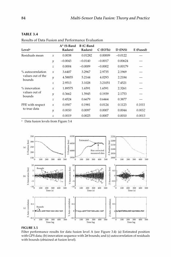
84 Multi-Sensor Data Fusion: Theory and Practice

FIGURE 3.5 Filter performance results for data fusion level A (see Figure 3.4): (a) Estimated position

with GPS data; (b) innovation sequence with 2σ bounds; and (c) autocorrelation of residuals

with bounds (obtained at fusion level).

350

(a)

(b)

(c)

X-Po

sitio

n (k

m)

250

150 0 100 200 300 400 500 0 100 200 300 400 500 0 100 200 300 400 500

0 100 200 300Time (s) Time (s) Time (s)

Time lagTime lagTime lag

400 500 0 100 200 300 400 500 0 100 200 300 400 500

0 100 200 300 400 500 0 100 200 300 400 500 0 100 200 300 400 500

300

200

10

X-In

nova

tion

(km

)

0

−10

5

−5

1

X Au

to-c

orre

latio

n

0

0.5

−0.5

1

Y Au

to-c

orre

latio

n

0

0.5

−0.5

1

Z-In

nova

tion

(km

)

0

0.5

−0.5

−1

1

Z Au

to-c

orre

latio

n

0

0.5

−0.5

10

Y-In

nova

tion

(km

)

0

−10

5

−5

6100Estimated

Bias correctedmeasured data

Bounds

Bounds

Y-Po

sitio

n (k

m)

6000

6050

5950

2250

Z-Po

sitio

n (k

m)

2150

2100

2050

2200

2000

TABLE 3.4

Results of Data Fusion and Performance Evaluation

Levela

A* (S-Band

Radars)

B (C-Band

Radars) C (EOTs) D (INS) E (Fused)

Residuals mean x 0.0038 0.01282 0.00009 −0.0122 —

y −0.0043 −0.0140 −0.0017 0.00624 —

z 0.0004 −0.0009 −0.0002 0.00179 —

% autocorrelation

values out of the

bounds

x 3.6407 3.2967 2.9735 2.1969 —

y 4.58855 5.2144 4.0293 2.2184 —

z 2.9513 3.1028 3.21051 7.4521 —

% innovation

values out of

bounds

x 1.89575 1.6591 1.6591 2.3261 —

y 0.3662 1.5945 0.1939 2.1753 —

z 0.4524 0.6679 0.6464 0.3877 —

PFE with respect

to true data

x 0.0987 0.1981 0.0124 0.1123 0.1011

y 0.0050 0.0097 0.0007 0.0044 0.0052

z 0.0019 0.0025 0.0007 0.0010 0.0013a Data fusion levels from Figure 3.4

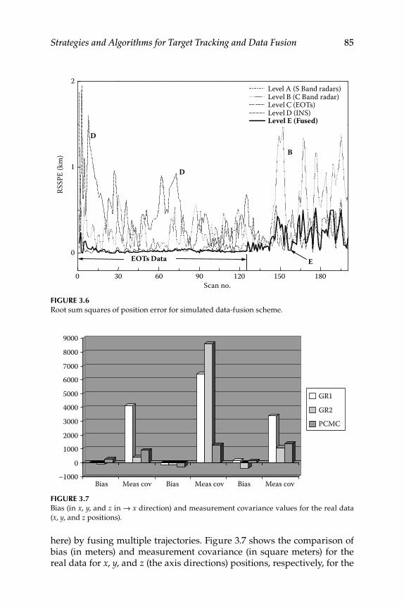
Strategies and Algorithms for Target Tracking and Data Fusion 85

here) by fusing multiple trajectories. Figure 3.7 shows the comparison of bias (in meters) and measurement covariance (in square meters) for the real data for x , y , and z (the axis directions) positions, respectively, for the

FIGURE 3.6 Root sum squares of position error for simulated data-fusion scheme.

1801501209060300

0

1

2

EEOTs Data

D

D

B

Scan no.

RSSP

E (k

m)

Level A (S Band radars)Level B (C Band radar)Level C (EOTs)Level D (INS)Level E (Fused)

−10000

10002000

3000

40005000

60007000

8000

9000

Bias Meas cov Bias Meas cov Bias Meas cov

GR1

GR2PCMC

FIGURE 3.7 Bias (in x , y , and z in → x direction) and measurement covariance values for the real data

( x , y , and z positions).

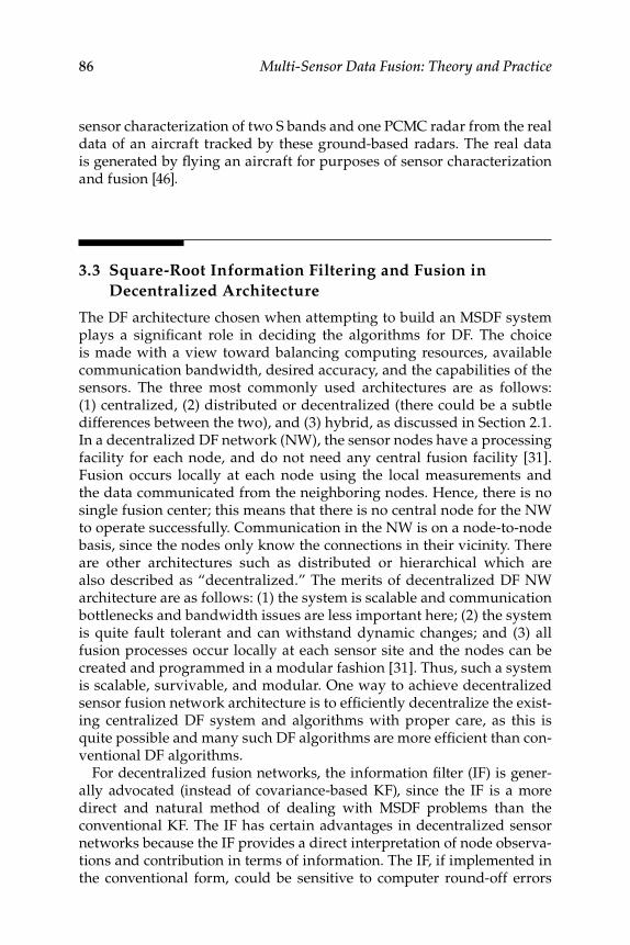
86 Multi-Sensor Data Fusion: Theory and Practice

sensor characterization of two S bands and one PCMC radar from the real data of an aircraft tracked by these ground-based radars. The real data is generated by fl ying an aircraft for purposes of sensor characterization and fusion [46].

3.3 Square-Root Information Filtering and Fusion in

Decentralized Architecture

The DF architecture chosen when attempting to build an MSDF system plays a signifi cant role in deciding the algorithms for DF. The choice is made with a view toward balancing computing resources, available communication bandwidth, desired accuracy, and the capabilities of the sensors. The three most commonly used architectures are as follows: (1) centralized, (2) distributed or decentralized (there could be a subtle differences between the two), and (3) hybrid, as discussed in Section 2.1. In a decentralized DF network (NW), the sensor nodes have a processing facility for each node, and do not need any central fusion facility [31]. Fusion occurs locally at each node using the local measurements and the data communicated from the neighboring nodes. Hence, there is no single fusion center; this means that there is no central node for the NW to operate successfully. Communication in the NW is on a node-to-node basis, since the nodes only know the connections in their vicinity. There are other architectures such as distributed or hierarchical which are also described as “decentralized.” The merits of decentralized DF NW architecture are as follows: (1) the system is scalable and communication bottlenecks and bandwidth issues are less important here; (2) the system is quite fault tolerant and can withstand dynamic changes; and (3) all fusion processes occur locally at each sensor site and the nodes can be created and programmed in a modular fashion [31]. Thus, such a system is scalable, survivable, and modular. One way to achieve decentralized sensor fusion network architecture is to effi ciently decentralize the exist-ing centralized DF system and algorithms with proper care, as this is quite possible and many such DF algorithms are more effi cient than con-ventional DF algorithms.

For decentralized fusion networks, the information fi lter (IF) is gener-ally advocated (instead of covariance-based KF), since the IF is a more direct and natural method of dealing with MSDF problems than the conventional KF. The IF has certain advantages in decentralized sensor networks because the IF provides a direct interpretation of node observa-tions and contribution in terms of information. The IF, if implemented in the conventional form, could be sensitive to computer round-off errors

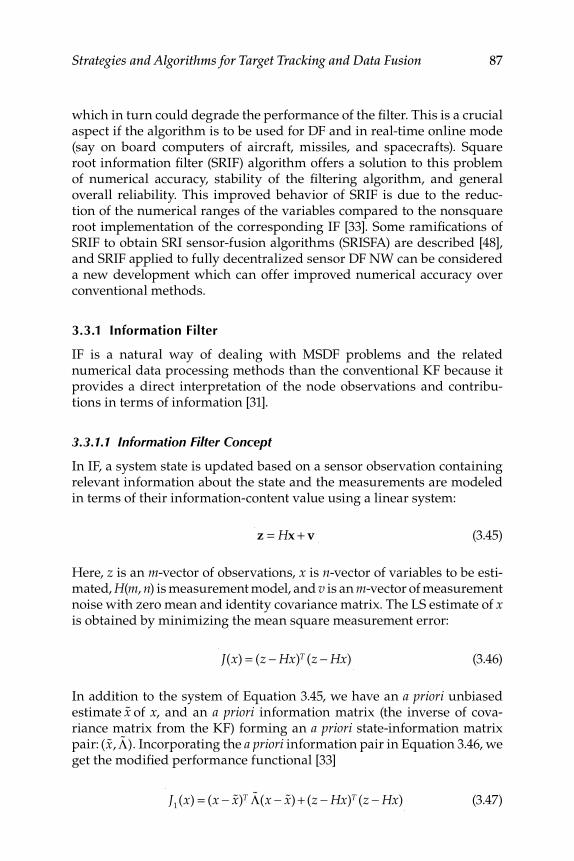
Strategies and Algorithms for Target Tracking and Data Fusion 87

which in turn could degrade the performance of the fi lter. This is a crucial aspect if the algorithm is to be used for DF and in real-time online mode (say on board computers of aircraft, missiles, and spacecrafts). Square root information fi lter (SRIF) algorithm offers a solution to this problem of numerical accuracy, stability of the fi ltering algorithm, and general overall reliability. This improved behavior of SRIF is due to the reduc-tion of the numerical ranges of the variables compared to the nonsquare root implementation of the corresponding IF [33]. Some ramifi cations of SRIF to obtain SRI sensor-fusion algorithms (SRISFA) are described [48], and SRIF applied to fully decentralized sensor DF NW can be considered a new development which can offer improved numerical accuracy over conventional methods.

3.3.1 Information Filter

IF is a natural way of dealing with MSDF problems and the related numerical data processing methods than the conventional KF because it provides a direct interpretation of the node observations and contribu-tions in terms of information [31].

3.3.1.1 Information Filter Concept

In IF, a system state is updated based on a sensor observation containing relevant information about the state and the measurements are modeled in terms of their information-content value using a linear system:

z = Hx + v (3.45)

Here, z is an m -vector of observations, x is n -vector of variables to be esti-mated, H ( m , n ) is measurement model, and v is an m -vector of measurement noise with zero mean and identity covariance matrix. The LS estimate of x is obtained by minimizing the mean square measurement error:

J(x) = (z − Hx)T (z − Hx) (3.46)

In addition to the system of Equation 3.45, we have an a priori unbiased estimate %x of x , and an a priori information matrix (the inverse of cova-riance matrix from the KF) forming an a priori state-information matrix pair: ( %x, %Λ). Incorporating the a priori information pair in Equation 3.46, we get the modifi ed performance functional [33]

J1(x) = (x − %x)T %Λ(x − %x) + (z − Hx)T (z − Hx) (3.47)

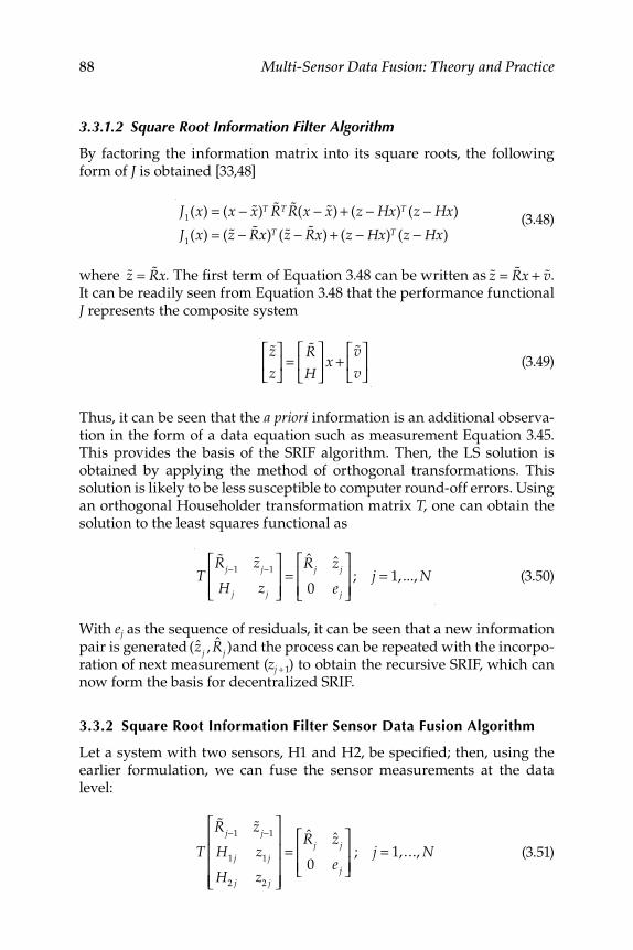
88 Multi-Sensor Data Fusion: Theory and Practice

3.3.1.2 Square Root Information Filter Algorithm

By factoring the information matrix into its square roots, the following form of J is obtained [33,48]

J1(x) = (x − %x)T %RT %R(x − %x) + (z − Hx)T (z − Hx)

J1(x) = ( %z − %Rx)T ( %z − %Rx) + (z − Hx)T (z − Hx)

(3.48)

w here %z = %Rx . The fi rst term of Equation 3.48 can be written as %z = %Rx + %v. It can be readily seen from Equation 3.48 that the performance functional J represents the composite system

%zz

⎡

⎣⎢

⎤

⎦⎥ =

%RH

⎡

⎣⎢

⎤

⎦⎥ x +

%vv

⎡

⎣⎢

⎤

⎦⎥ (3.49)

Thus, it can be seen that the a priori information is an additional observa-tion in the form of a data equation such as measurement Equation 3.45. This provides the basis of the SRIF algorithm. Then, the LS solution is obtained by applying the method of orthogonal transformations. This solution is likely to be less susceptible to computer round-off errors. Using an orthogonal Householder transformation matrix T , one can obtain the solution to the least squares functional as

T%Rj−1

%zj−1

H j zj

⎡

⎣⎢⎢

⎤

⎦⎥⎥

=Rj z j

0 ej

⎡

⎣⎢⎢

⎤

⎦⎥⎥

; j = 1,..., N (3.50)

With e j as the sequence of residuals, it can be seen that a new information pair is generated (z j , Rj )and the process can be repeated with the incorpo-ration of next measurement ( z j + 1 ) to obtain the recursive SRIF, which can now form the basis for decentralized SRIF.

3.3.2 Square Root Information Filter Sensor Data Fusion Algorithm

Let a system with two sensors, H1 and H2, be specifi ed; then, using the earlier formulation, we can fuse the sensor measurements at the data level:

T

%Rj−1%zj−1

H1 j z1 j

H2 j z2 j

⎡

⎣

⎢⎢⎢⎢

⎤

⎦

⎥⎥⎥⎥

=Rj zj

0 e j

⎡

⎣⎢⎢

⎤

⎦⎥⎥

; j = 1,..., N (3.51)

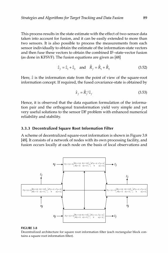
Strategies and Algorithms for Target Tracking and Data Fusion 89

This process results in the state estimate with the effect of two-sensor data taken into account for fusion, and it can be easily extended to more than two sensors. It is also possible to process the measurements from each sensor individually to obtain the estimate of the information-state vectors and then fuse these vectors to obtain the combined IF–state-vector fusion (as done in KFSVF). The fusion equations are given as [48]

z f = z

1+ z

2and R f = R

1+ R

2 (3.52)

Here, z is the information state from the point of view of the square-root information concept. If required, the fused covariance-state is obtained by

x f = R f

−1z f (3.53)

Hence, it is observed that the data equation formulation of the informa-tion pair and the orthogonal transformation yield very simple and yet very useful solutions to the sensor DF problem with enhanced numerical reliability and stability.

3.3.3 Decentralized Square Root Information Filter

A scheme of decentralized square-root information is shown in Figure 3.8 [48]. It consists of a network of nodes with its own processing facility, and fusion occurs locally at each node on the basis of local observations and

FIGURE 3.8 Decentralized architecture for square root information fi lter (each rectangular block con-

tains a square root information fi lter).

e(j + 1)0z*(j + 1)R*(j + 1)

z(j + 1)H(j + 1)z(j + 1/j) =R(j + 1/j)T(j + 1/j + 1)

e(j + 1)0z*(j + 1)R*(j + 1)

z(j + 1)H(j + 1)z(j + 1/j) =R(j + 1/j)T(j + 1/j + 1)

e(j + 1)0z*(j + 1)R*(j + 1)

z(j + 1)H(j + 1)z(j + 1/j) =R(j + 1/j)T(j + 1/j + 1)

e(j + 1)0z*(j + 1)R*(j + 1)

z(j + 1)H(j + 1)z(j + 1/j) =R(j + 1/j)T (j + 1/j + 1)

zj zj

zj

zj

zj

zj

zj zj

90 Multi-Sensor Data Fusion: Theory and Practice

the information communicates from neighboring nodes [31,48]. The pro-cessing node is a sensor-fusion node that takes local observations and shares information with other fusion nodes. It assimilates the communi-cated information and computes the estimate.

A linear system is given in state equation form as

x( j + 1) = Φx( j) + Gw( j) (3.54)

Here, w is the white Gaussian process noise with zero mean and covari-ance Q . It is assumed that the a priori information given about x 0 and w 0 can be put in data equation as [48]

zw = Rww

0+ νw (3.55)

%z

0= %R

0x

0+ %ν

0 (3.56)

Here, the variables ν0, %ν

0, and νw are assumed to be zero mean, indepen-

dent, and with unity covariance matrices. By incorporating the a priori information, the time propagation part of the SRIF obtains the following form. The local mapping (time propagation) is given as [48]

T( j + 1)

%Rw ( j) 0 %zw ( j)

−Rd ( j + 1)G Rd ( j + 1) %z( j)

⎡

⎣⎢

⎤

⎦⎥ =

Rw ( j + 1) Rwx ( j + 1) zw ( j + 1)

0 R( j + 1) z( j + 1)

⎡

⎣⎢

⎤

⎦⎥

(3.57)

The subscript w signifi es the variables related to the process noise. We have

R

d ( j + 1) = R( j)ϕ−1( j + 1) (3.58)

Local estimates are generated using measurement update of SRIF [48]

T j + 1 j + 1( ) R( j + 1/j) z( j + 1/j)

H( j + 1) z( j + 1)

⎡

⎣⎢

⎤

⎦⎥ =

R* ( j + 1) z* ( j + 1)

0 e( j + 1)

⎡

⎣⎢

⎤

⎦⎥ (3.59)

Here, * denotes the local updated estimates. These estimates can be com-municated between all nodes in a fully connected network, and at each node the estimates can be assimilated to produce global SRIF estimates. Assimilation equations to produce global SRI estimates at the i th node (with k = 1, …, N − 1 representing the remaining nodes) are given by [48]

Strategies and Algorithms for Target Tracking and Data Fusion 91

zi j + 1/j + 1( ) = z* j + 1/j + 1( ) + zk

* j + 1/j + 1( )k=1

N −1

∑ (3.60)

Ri j + 1/j + 1( ) = R* j + 1/j + 1( ) + Rk

* j + 1/j + 1( )k=1

N −1

∑ (3.61)

This formulation of the information pair and the orthogonal transforma-tion T, in the data equation format, yields in a natural way very elegant, simple, and useful solutions to the decentralized sensor DF problem. The algorithm would possess better numerical reliability and stability due to the use of the square-root fi ltering formulation compared to the normal IF-based schemes. The basic ramifi cations, such as inclusion of correlated process noise and bias parameters (from the IF/SRIF [33]), are equally applicable to the decentralized SRISFA (DSRISFA) and in SRIF structure it is easy to derive algorithm modifi cations and/or approximations with the data equation framework in a straightforward manner. Decentralized IF for fusion requires communication of the local “information states” and information matrices to all the neighboring nodes for computing the global estimates, whereas in the case of the SRIF for fusion the informa-tion states and information matrices are estimated together. Communica-tion between local nodes involves the transmission of the fi rst row of the matrix (RHS of Equation 3.59) as a whole in a fully decentralized network with a number of nodes. The smaller range of numbers in the SRIF for-mulation enables the results to be represented by fewer bits. This would result in communications overhead savings.

3.3.4 Numerical Simulation Results

Numerically simulated data of the position of a target moving with con-stant acceleration are generated. The decentralized SRISFA is validated for a two-node interconnection network. The system has position, velocity, and acceleration as its states

xT = [x &x &&x] (3.62)

With the transition matrix as follows:

Φ =1 Δt Δt2/2

0 1 Δt

0 0 1

⎡

⎣

⎢⎢⎢

⎤

⎦

⎥⎥⎥

; G =Δt3/6

Δt2/2

Δt

⎡

⎣

⎢⎢⎢

⎤

⎦

⎥⎥⎥

(3.63)

92 Multi-Sensor Data Fusion: Theory and Practice

The Δ t is sampling interval of 0.5 s, and w is white Gaussian noise with zero mean and standard deviation of 0.0001. The measurement model for each sensor is given by

zm( j + 1) = Hx( j + 1) + vm( j + 1) (3.64)

Here, H = [1 0 0] for each sensor. The vector v is measurement noise, and white Gaussian noise with zero mean. The position data pertaining to the two nodes or measuring sensors are generated by adding random noise with σv1

= 1 and σv2= 5. The whitened measurements with appropriate mea-

surement equations are used for generating fused global estimates at both the nodes. This is done by utilizing the local estimates at the node and the communicated information from the neighboring nodes. The performance of the SRIFDF algorithm in terms of numerical accuracy is compared with the decentralized information fi lter algorithm for two nodes imple-mented in PC MATLAB® using the simulated data. Both the algorithms were started with identical initial conditions (for the state and informa-tion matrices) and with the same values of process and measurement noise covariance. Table 3.5 gives the PFE of the state estimation error for three states obtained using SRI fi lter and IF algorithms. The fi t error is calculated using PFE = 100 * norm(x − xt )/norm(xt )where x t is the true state. It is clear that the PFEs are lower when the SRIF algorithm is used for estimation. It is also clear that the SRIF is relatively less sensitive to variation in Q when compared with IF. Subsequently, the SRIF was applied to certain real-fl ight test data of a launch vehicle obtained from two ground radars (placed at different locations). The radars measure the range, azimuth, and elevation of the moving vehicle. These data are converted to Cartesian coordinate frame so that linear-state and measurement models can be used. The data are converted to a common reference point and whitened before use in state estimation or fusion exercises. Kinematic fusion is performed after processing the data using SRIF at each node. The norms of the SRI matrix, which is a direct outcome of the SRIF algorithm, are compared for indi-vidual sensors and for fused data for all the axes. The norms for the fused data were higher than those of the individual sensors. The detailed results for four nodes of SRIFDF can be found in [48].

TABLE 3.5

Performance Metrics for Local Nodes and Global Fused Estimate (Qii = 1.0e-4)

PFE for SRIF for [x &x &&x] PFE for IF [x &x &&x]

Node 1 0.0212 0.3787 3.8768 0.0342 0.8637 13.8324

Node 2 0.0931 0.6771 4.6231 0.1274 2.2168 20.9926

Fused 0.0294 0.4012 3.9470 0.0338 0.8456 13.4540

Strategies and Algorithms for Target Tracking and Data Fusion 93

3.4 Nearest Neighbor and Probabilistic Data Association

Filter Algorithms

We have seen that gating and DA operations are required to enable effi -cient tracking in MSMT scenario. Gating helps in deciding if an obser-vation (which might include clutter, false alarms, electronic counter measures, and so on) is a probable candidate for track maintenance or track update. DA is a step to associate the measurements to the targets with certainty when several targets are in the same neighborhood. Now, two approaches to DA and related fi ltering algorithms will be discussed [38,39]:

1. The nearest neighbor (NN) approach, in which a unique pairing is determined. At most one observation can be paired with an ear-lier established track; the goal is to minimize an overall distance function that considers all observation-to-track pairings that sat-isfy a preliminary gating test.

2. The PDAF algorithm, in which a track is updated based on the decision using a weighted sum of innovations from multiple vali-dated measurements.

A program based on gating and DA using both NNKF and PDAF approaches has been developed in PC MATLAB for handling the prob-lem of tracking in a MSMT scenario. It is primarily an adapted version of the commercially available software package [41] and is updated and modifi ed for the present application. The salient features of the upgraded MSMT packages are [40] (1) data are transformed to common reference point; (2) both NNKF and PDAF are used; (3) similar tracks are combined; (4) direction feature is included; (5) performance metrics Singer–Kanyuck (S–K), RMSPE, and RSSPE are evaluated; and (6) the track loss feature is also included. In Figure 3.9, the steps of the MSMT program are shown [40]. The test scenarios considered are

1. Three targets launched from different sites and nine sensors located at different locations tracking these targets, and the three sensors are confi gured to track one target. The program generates information on the target-sensor lock status. The performance is evaluated by adding clutter to the data and simulating the data loss in one or more of the sensors for a short time period.

2. Each of the three sensors looks at six targets and then all the three sensor results are fused, with the possibility of some data loss.

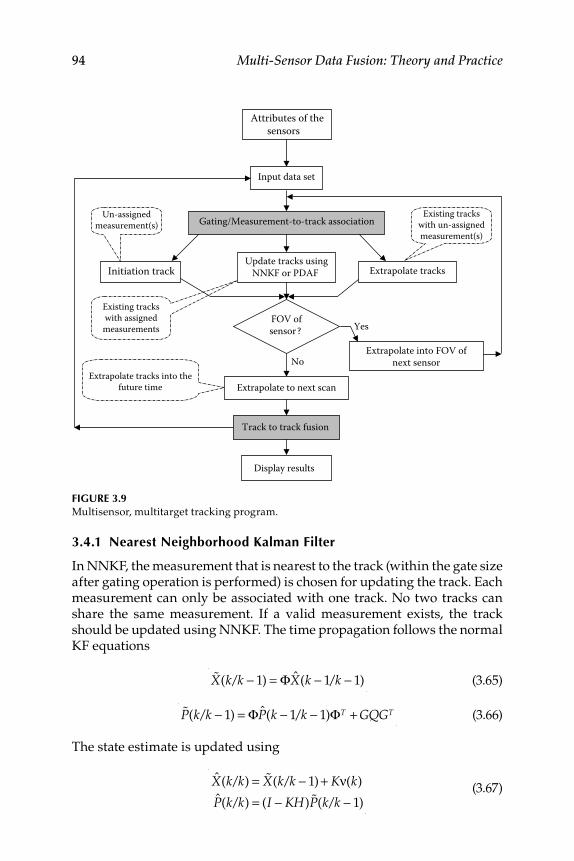
94 Multi-Sensor Data Fusion: Theory and Practice

3.4.1 Nearest Neighborhood Kalman Filter

In NNKF, the measurement that is nearest to the track (within the gate size after gating operation is performed) is chosen for updating the track. Each measurement can only be associated with one track. No two tracks can share the same measurement. If a valid measurement exists, the track should be updated using NNKF. The time propagation follows the normal KF equations

%X(k/k − 1) = ΦX(k − 1/k − 1) (3.65)

%P(k/k − 1) = ΦP(k − 1/k − 1)ΦT + GQGT (3.66)

The state estimate is updated using

X(k/k) = %X(k/k − 1) + Kν(k)

P(k/k) = (I − KH) %P(k/k − 1) (3.67)

FIGURE 3.9 Multisensor, multitarget tracking program.

No

Yes

Input data set

Gating/Measurement-to-track association

Update tracks usingNNKF or PDAF Initiation track Extrapolate tracks

Existing trackswith un-assignedmeasurement(s)

Track to track fusion

Display results

Attributes of thesensors

FOV ofsensor?

Extrapolate to next scanExtrapolate tracks into the

future time

Un-assignedmeasurement(s)

Extrapolate into FOV ofnext sensor

Existing tracks with assigned measurements

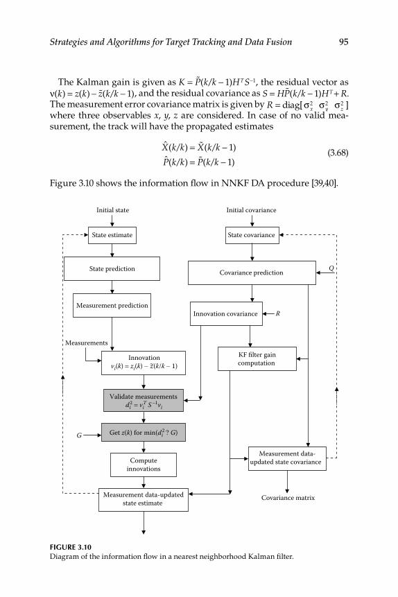
Strategies and Algorithms for Target Tracking and Data Fusion 95

The Kalman gain is given as K = %P(k/k − 1)HTS−1, the residual vector as

ν(k) = z(k) − %z(k/k − 1), and the residual covariance as S = H %P(k/k − 1)HT + R. The measurement error covariance matrix is given by

R = diag[σx2 σy

2 σz2 ]

where three observables x , y , z are considered. In case of no valid mea-surement, the track will have the propagated estimates

X(k/k) = %X(k/k − 1)

P(k/k) = %P(k/k − 1) (3.68)

Figure 3.10 shows the information fl ow in NNKF DA procedure [39,40].

FIGURE 3.10 Diagram of the information fl ow in a nearest neighborhood Kalman fi lter.

Initial covariance Initial state

G

Q

R

State estimate State covariance

State prediction Covariance prediction

Measurement predictionInnovation covariance

Innovationvi(k) = zi(k) - ~z(k/k - 1)

Validate measurementsdi

2 = viT S -1vi

KF filter gaincomputation

Measurement data-updated state covariance

Measurement data-updatedstate estimate

Measurements

Get z(k) for min(di2 ? G)

Computeinnovations

Covariance matrix

96 Multi-Sensor Data Fusion: Theory and Practice

3.4.2 Probabilistic Data Association Filter

The PDAF algorithm computes the association probabilities for each valid measurement at the current instant for the target; this information is used in the fi lter. If it is assumed that there are m measurements falling within a particular gate, that there is only one target of interest, and that the track has been initialized [38,40–43], then the association events as below are mutually exclusive and exhaustive for m ≥ 1.

zi = { yi is the target originated measurement}, i = 1, 2, ..., m,

{none of the measurements is target originated}, i = 0

(3.69)

The conditional mean of the state is written as

X(k/k) = Xi (k/k)pi

i=0

m

∑ (3.70)

Here, Xi (k/k) is the updated state that is conditioned on the event that the i th validated measurement is correct and pi is the conditional probabil-ity of the event. The estimates conditioned on the measurement i , being assumed to be correct, are given by

Xi (k/k) = %X(k/k − 1) + Kνi (k), i = 1, 2,…, m (3.71)

and the conditional innovation are given by

νi (k) = zi (k) − z(k/k − 1) (3.72)

For i = 0, if none of the measurements is valid ( m = 0) then

X0(k/k) = %X(k/k − 1) (3.73)

The state update equation of the PDAF is given as

X(k/k) = %X(k/k − 1) + Kν(k) (3.74)

The merged innovation expression is given by

ν(k) = pi (k)

i=1

m

∑ νi (k) (3.75)

The covariance matrix associated with the updated state is given as

P(k/k) = p

0(k) %P(k/k − 1) + 1 − p

0(k)( ) Pc(k/k) + Ps(k) (3.76)

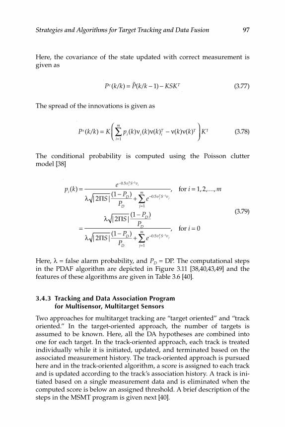
Strategies and Algorithms for Target Tracking and Data Fusion 97

Here, the covariance of the state updated with correct measurement is given as

Pc (k/k) = %P(k/k − 1) − KSKT (3.77)

The spread of the innovations is given as

Ps (k/k) = K pi (k)

i=1

m

∑ νi (k)ν(k)iT − ν(k)ν(k)T

⎛⎝⎜

⎞⎠⎟

KT (3.78)

The conditional probability is computed using the Poisson clutter model [38]

pi (k) = e−0.5viTS−1vi

λ |2ΠS|(1 − PD )

PD

+ e−0.5vjTS−1vj

j=1

m

∑, for i = 1, 2, ..., m

=λ |2ΠS|

(1 − PD )

PD

λ |2ΠS|(1 − PD )

PD

+ e−0.5vjTS−1vj

j=1

m

∑, for i = 0

(3.79)

Here, λ = false alarm probability, and P D = DP. The computational steps in the PDAF algorithm are depicted in Figure 3.11 [38,40,43,49] and the features of these algorithms are given in Table 3.6 [40].

3.4.3 Tracking and Data Association Programfor Multisensor, Multitarget Sensors

Two approaches for multitarget tracking are “target oriented” and “track oriented.” In the target-oriented approach, the number of targets is assumed to be known. Here, all the DA hypotheses are combined into one for each target. In the track-oriented approach, each track is treated individually while it is initiated, updated, and terminated based on the associated measurement history. The track-oriented approach is pursued here and in the track-oriented algorithm, a score is assigned to each track and is updated according to the track’s association history. A track is ini-tiated based on a single measurement data and is eliminated when the computed score is below an assigned threshold. A brief description of the steps in the MSMT program is given next [40].

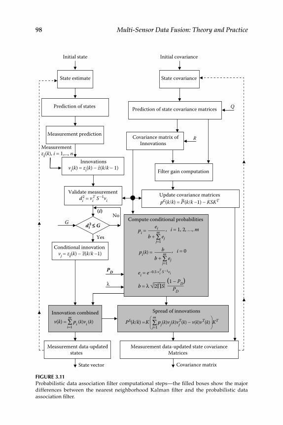
98 Multi-Sensor Data Fusion: Theory and Practice

FIGURE 3.11 Probabilistic data association fi lter computational steps—the fi lled boxes show the major

differences between the nearest neighborhood Kalman fi lter and the probabilistic data

association fi lter.

(i)

PD

No

Yes

Covariance matrix State vector

Initial state Initial covariance

G

Q

R

State estimate State covariance

Prediction of states Prediction of state covariance matrices

Measurement prediction Covariance matrix ofInnovations

Filter gain computation

Measurement data-updated state covarianceMatrices

Measurement data-updatedstates

Conditional innovation vj = zi(k) - ~z(k/k -1)

Update covariance matricespc(k/k) = P~ (k/k -1) - KSKT

λ

Measurementzi (k), i = 1,..., n

di2 ≤ G

Innovationsvi(k) = zi(k) - z(k/k - 1)

Validate measurementdi

2 = viT S -1vi

Spread of innovations

PS(k/k) =K Sm

pj(k)vj (k)vjT(k) - v(k)vT(k) KT

j=1

Innovation combined v(k) = S

m pi (k)vi (k)

i=1

Compute conditional probabilities

pi =

ei = e-0.5 vTi S -1vi

b = λ √⎯⎯

(1 - PD)PD

|2ÕS|

pi(k) = , i = 0

j=1b + S

m ej

b

, i = 1, 2, . . ., m

j=1b + S

m ej

ei

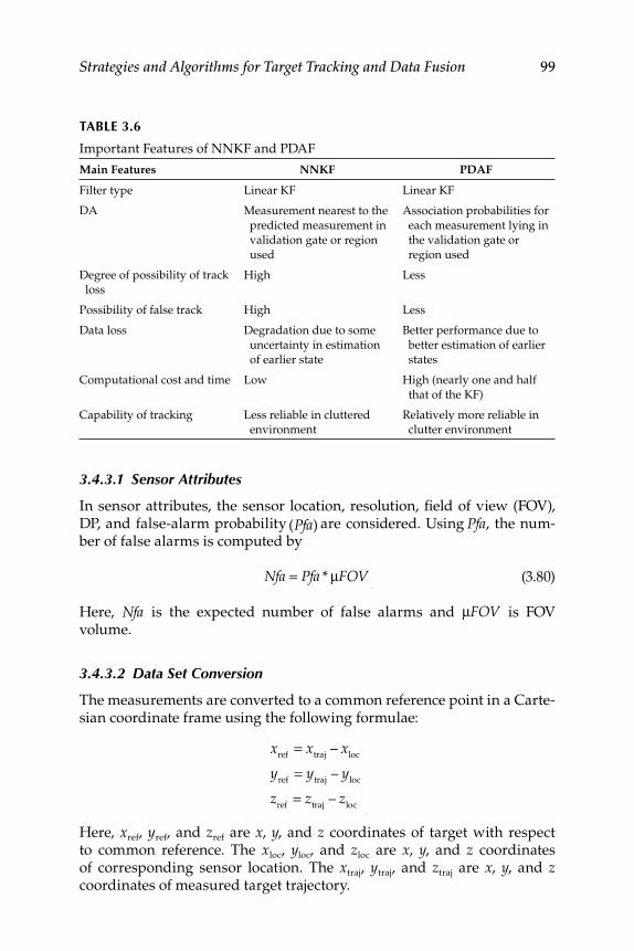
Strategies and Algorithms for Target Tracking and Data Fusion 99

3.4.3.1 Sensor Attributes

In sensor attributes, the sensor location, resolution, fi eld of view (FOV), DP, and false-alarm probability (Pfa) are considered. Using Pfa, the num-ber of false alarms is computed by

Nfa = Pfa * μFOV (3.80)

Here, Nfa is the expected number of false alarms and μFOV is FOV volume.

3.4.3.2 Data Set Conversion

The measurements are converted to a common reference point in a Carte-sian coordinate frame using the following formulae:

xref

= xtraj

– xloc

yref

= ytraj

– yloc

zref

= ztraj

– zloc

Here, x ref , y ref , and z ref are x , y , and z coordinates of target with respect to common reference. The x loc , y loc , and z loc are x , y , and z coordinates of corresponding sensor location. The x traj , y traj , and z traj are x , y , and z coordinates of measured target trajectory.

TABLE 3.6

Important Features of NNKF and PDAF

Main Features NNKF PDAF

Filter type Linear KF Linear KF

DA Measurement nearest to the

predicted measurement in

validation gate or region

used

Association probabilities for

each measurement lying in

the validation gate or

region used

Degree of possibility of track

loss

High Less

Possibility of false track High Less

Data loss Degradation due to some

uncertainty in estimation

of earlier state

Better performance due to

better estimation of earlier

states

Computational cost and time Low High (nearly one and half

that of the KF)

Capability of tracking Less reliable in cluttered

environment

Relatively more reliable in

clutter environment

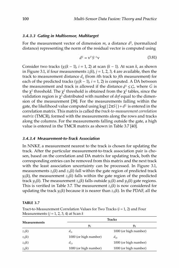
100 Multi-Sensor Data Fusion: Theory and Practice

3.4.3.3 Gating in Multisensor, Multitarget

For the measurement vector of dimension m , a distance d2 , (normalized distance) representing the norm of the residual vector is computed using

d2 = νTS−1ν (3.81)

Consider two tracks ( y i ( k − 1), i = 1, 2) at scan ( k − 1). At scan k , as shown in Figure 3.1, if four measurements z j ( k ), j = 1, 2, 3, 4 are available, then the track to measurement distance d ij (from i th track to j th measurement) for each of the predicted tracks ( y i ( k − 1), i = 1, 2) is computed. A DA between the measurement and track is allowed if the distance d

2 ≤ G, where G is the χ 2 threshold. The χ 2 threshold is obtained from the χ 2 tables, since the validation region is χ 2 distributed with number of dof equal to the dimen-sion of the measurement [38]. For the measurements falling within the gate, the likelihood value computed using log(|2πS|) + d2 is entered in the correlation matrix. This matrix is called the track-to-measurement correlation matrix (TMCR), formed with the measurements along the rows and tracks along the columns. For the measurements falling outside the gate, a high value is entered in the TMCR matrix as shown in Table 3.7 [40].

3.4.3.4 Measurement-to-Track Association

In NNKF, a measurement nearest to the track is chosen for updating the track. After the particular measurement-to-track association pair is cho-sen, based on the correlation and DA matrix for updating track, both the corresponding entries can be removed from this matrix and the next track with the least association uncertainty can be processed. In Figure 3.1, measurements z 1 ( k ) and z 3 ( k ) fall within the gate region of predicted track y 1 ( k ), the measurement z 2 ( k ) falls within the gate region of the predicted track y 2 ( k ). The measurement z 4 ( k ) falls outside y 1 ( k ) and y 2 ( k ) gate regions. This is verifi ed in Table 3.7. The measurement z 1 ( k ) is now considered for updating the track y 1 ( k ) because it is nearer than z 3 ( k ). In the PDAF, all the

TABLE 3.7

Tract-to-Measurement Correlation Values for Two Tracks (i = 1, 2) and Four Measurements (j = 1, 2, 3, 4) at Scan k

MeasurementsTracks

y1 y2

z1(k) d11 1000 (or high number)

z2(k) 1000 (or high number) d22

z3(k) d13 1000 (or high number)

z4(k) 1000 (or high number) 1000 (or high number)

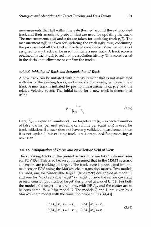
Strategies and Algorithms for Target Tracking and Data Fusion 101

measurements that fall within the gate (formed around the extrapolated track and their associated probabilities) are used for updating the track. The measurements z 1 ( k ) and z 3 ( k ) are taken for updating track y 1 ( k ). The measurement z 2 ( k ) is taken for updating the track y 2 ( k ), thus, continuing the process until all the tracks have been considered. Measurements not assigned to any track can be used to initiate a new track. A track score is obtained for each track based on the association history. This score is used in the decision to eliminate or confi rm the tracks.

3.4.3.5 Initiation of Track and Extrapolation of Track

A new track can be initiated with a measurement that is not associated with any of the existing tracks, and a track score is assigned to each new track. A new track is initiated by position measurements ( x , y , z ) and the related velocity vector. The initial score for a new track is determined using

p =

βNT

βNT

+ βfa

(3.82)

Here, β NT = expected number of true targets and β fa = expected number of false alarms (per unit surveillance volume per scan). z 4 ( k ) is used for track initiation. If a track does not have any validated measurement, then it is not updated, but existing tracks are extrapolated for processing at next scan.

3.4.3.6 Extrapolation of Tracks into Next Sensor Field of View

The surviving tracks in the present sensor FOV are taken into next sen-sor FOV [38]. This is so because it is assumed that in the MSMT scenario all sensors are tracking all targets. The track score is propagated into the next sensor FOV using the Markov chain transition matrix. Two models are used, one for “observable target” (true track) designated as model O and one for “unobservable target” (a target outside the sensor coverage or erroneously hypothesized target) designated as model U [41]. For both the models, the target measurements, with DP P D , and the clutter are to be considered. P D = 0 for model U. The models O and U are given by a Markov chain model with the transition probabilities [41,43]

P(MO MO ) = 1 − εO , P(MU MO ) = εO

P(MU MU ) = 1 − εU , P(MO MU ) = εU

(3.83)

102 Multi-Sensor Data Fusion: Theory and Practice

Here, Mx denotes the event that the model ‘ x ’ is in effect during the cur-rent sampling interval and MX is for the earlier interval. The exact values of ε A and ε D can be chosen based on the problem scenario under study.

3.4.3.7 Extrapolation of Tracks into Next Scan

The valid and surviving tracks are extrapolated at the next scan using a target model given as follows:

X(k + 1) = FX(k) + Gw(k) (3.84)

Here, the target dynamic state transition matrix is given as

F =

1 0 0 Δt 0 0

0 1 0 0 Δt 0

0 0 1 0 0 Δt

0 0 0 1 0 0

0 0 0 0 1 0

0 0 0 0 0 1

⎡

⎣

⎢⎢⎢⎢⎢⎢⎢⎢

⎤

⎦

⎥⎥⎥⎥⎥⎥⎥⎥

The state vector is given by X(k) = [x(k) y(k) z(k) &x(k) &y(k) &z(k)]T . The process noise w ( k ) is assumed to be a zero-mean white Gaussian noise with covariance E[w(k)w(k)T ] = Q(k). Δt is the sampling interval. The pro-cess noise gain matrix is given as

G =

Δt2/2 0 0

0 Δt2/2 0

0 0 Δt2/2

Δt 0 0

0 Δt 0

0 0 Δt

⎡

⎣

⎢⎢⎢⎢⎢⎢⎢⎢

⎤

⎦

⎥⎥⎥⎥⎥⎥⎥⎥

The time propagation of the states and covariance matrices is performed using the KF-prediction equation.

3.4.3.8 Track Management Process

A scoring threshold is used to eliminate false tracks, and is one of the system design parameters. It can be adjusted based on the scenario and required performance. Similar tracks are fused to avoid redundant tracks. The direction of the tracks also has to be considered while merging

Strategies and Algorithms for Target Tracking and Data Fusion 103

similar tracks. An N D -scan approach is used [39]—the tracks that have the last N D observations in common are merged. Based on the value of N D , the approach would automatically take the velocity as well as acceleration into account for merging similar tracks; for example, x (2) − − x (1) can be regarded as velocity. A 3-scan approach is used by the MSMT program for merging the tracks. Consider two tracks with the state-vector estimates and the covariance matrices given at scan k

track i : Xi (k/k), Pi (k/k)

track j : X j (k/k), Pj (k/k) (3.85)

The merged or combined state vector is the usual state-vector fusion with

Xc (k) = Xi (k/k) + Pi (k/k)P(k)ij

−1 X j (k/k) − Xi (k/k)⎡⎣ ⎤⎦ (3.86)

and the combined covariance matrix is given as

Pc (k) = Pi (k/k) − Pi (k/k)P(k)ij

−1 Pi (k/k) (3.87)

P(k)ij = Pi (k/k) + Pj (k/k) (3.88)

The program logic would fi nally generate information regarding the surviving tracks and sensors to target lock status. The graphical display module displays the true trajectory and measurements and also perfor-mance measures such as true and false track detections, number of good and false tracks, and good and false track probabilities. It also displays the sensor and target lock status.

3.4.4 Numerical Simulation

The performance of the NNKF and PDAF is evaluated by computing: (1) the PFE in x , y , and z positions; (2) the RMSPE; (3) the RSSPE; (4) S–K track

association metric Cij = xi − x j(Pi +Pj )

−1

2

, Cij = (xi − x j )T (Pi + Pj )

−1(xi − x j ) (the

metric Cij [42] can be viewed as the square of the [normalized] distance between two Gaussian distributions with mean vectors xi and x j and a common covariance matrix Pi + Pj); and (5) percentage root mean square position error (RMSPE).

RMSPE = RMSPE

1

Nxi

2 + yi2 + zi

2

3i=1

N

∑* 100 (3.89)

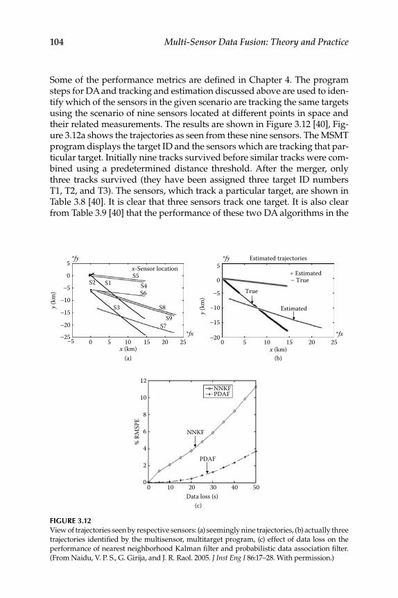
104 Multi-Sensor Data Fusion: Theory and Practice

Some of the performance metrics are defi ned in Chapter 4. The program steps for DA and tracking and estimation discussed above are used to iden-tify which of the sensors in the given scenario are tracking the same targets using the scenario of nine sensors located at different points in space and their related measurements. The results are shown in Figure 3.12 [40], Fig-ure 3.12a shows the trajectories as seen from these nine sensors. The MSMT program displays the target ID and the sensors which are tracking that par-ticular target. Initially nine tracks survived before similar tracks were com-bined using a predetermined distance threshold. After the merger, only three tracks survived (they have been assigned three target ID numbers T1, T2, and T3). The sensors, which track a particular target, are shown in Table 3.8 [40]. It is clear that three sensors track one target. It is also clear from Table 3.9 [40] that the performance of these two DA algorithms in the

FIGURE 3.12 View of trajectories seen by respective sensors: (a) seemingly nine trajectories, (b) actually three

trajectories identifi ed by the multisensor, multitarget program, (c) effect of data loss on the

performance of nearest neighborhood Kalman fi lter and probabilistic data association fi lter.

(From Naidu, V. P. S., G. Girija, and J. R. Raol. 2005. J Inst Eng I 86:17−28. With permission.)

(c)

12

10

8

% RM

SPE

4

6

2

00 10

Data loss (s)20 30 40 50

NNKF

NNKF

PDAF

PDAF

5*fy

S2 S1 S4S5x-Sensor location

S6

S8

S7S9

S3

2520151050-5

(a)

*fx

0

-5

-10

y (km

)

x (km)

-15

-20

-25

*fy Estimated trajectories

y (km

)

5

0

-5

-10

-15

-20 *fx

(b)

2520151050x (km)

True- True

Estimated

+ Estimated

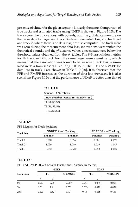
Strategies and Algorithms for Target Tracking and Data Fusion 105

presence of clutter for the given scenario is nearly the same. Comparison of true tracks and estimated tracks using NNKF is shown in Figure 3.12b. The track score, the innovations with bounds, and the χ distance measure on the x -axis data for target and track 1 (where there is data loss) and for target and track 2 (where there is no data loss) are also computed. The track score was zero during the measurement data loss, innovations were within the theoretical bounds, and the χ 2 distance values at each scan were below the threshold values obtained from the χ 2 tables. The S–K association metrics for i th track and j th track from the same target were almost zero, which means that the association was found to be feasible. Track loss is simu-lated in data from sensors 1–3 during 100–150 s. The PFE and RMSPE for data loss in track 1 are shown in Table 3.10 [40]. It is observed that the PFE and RMSPE increase as the duration of data loss increases. It is also seen from Figure 3.12c that the performance of PDAF is better than that of

TABLE 3.8

Sensor ID Numbers

Target Number (Sensor ID Number—ID)

T1 (S1, S2, S3)

T2 (S4, S5, S6)

T3 (S7, S8, S9)

TABLE 3.10

PFE and RMSPE (Data Loss in Track 1 and Distance in Meters)

Data Loss

NNKF PDAF

PFE % RMSPE PFE % RMSPE

x y x y

0 s 0.06 0.05 0.067 0.081 0.075 0.056

5 s 1.32 1.4 1.37 0.083 0.078 0.059

20 s 3.62 3.87 3.77 0.48 0.448 0.463

TABLE 3.9

PFE Metrics for Track Positions

Track No.NNKF DA and Tracking PDAF DA and Tracking

PFE in x PFE in y PFE in x PFE in y

Track 1 0.060 0.056 0.08 0.075

Track 2 1.039 1.049 1.039 1.049

Track 3 0.052 0.028 0.053 0.029

106 Multi-Sensor Data Fusion: Theory and Practice

NNKF in the presence of data loss. The data loss for longer time might be acceptable if PDAF is used. However, this depends on how much accuracy is required in overall tracking. The results of DF of 3-sensors and 6-targets (another test scenario) and associated performance aspects such as track probability, good tracks [38,43], and so on were obtained using the same MSMT program. Correct association and fusion of trajectories from differ-ent sensors were also obtained, and more details are given in [40].

3.5 Interacting Multiple Model Algorithm for

Maneuvering Target Tracking

Target tracking is more diffi cult if the target in motion is also maneuver-ing. KF has some ability to adapt to maneuvers by tuning the process noise covariance (and perhaps to some extent measurement noise- covariance) matrices, if the target is mildly maneuvering. The fi lter tuning could be either manual or automatic. Manual tuning means that the KF has been properly evaluated offl ine with postfl ight data already available. How-ever, for any new scenario this might not be the case. In such situations, trial and error method or automatic tuning has to be used. Thus, in a mul-titarget tracking system, a KF can be used for relatively benign maneuvers and an adequate noise reduction can be used for the periods when target is not maneuvering. In most situations, an interacting multiple-model KF (IMMKF) has been found to perform better than a KF [50,51]. The IMMKF uses a few target motion models (constant velocity, constant acceleration, coordinate turn model, and so on). For example, the IMMKF may use one model for a straight and level fl ight and different models for maneuvers or turns. The IMMKF always maintains the repository of all the models and blends their outputs with certain weighting coeffi cients that are computed probabilistically as part of the algorithm. In addition to the state estimates for each motion model, the IMMKF maintains an estimate of the probabil-ity with which the target is moving in accordance with each model.

3.5.1 Interacting Multiple Model Kalman Filter Algorithm

Thus, the IMMKF uses (1) several possible models for the target’s motion, and (2) a probabilistic switching mechanism between these models. It is implemented with multiple parallel (not in the real sense of parallelism or on parallel computers, however this is feasible and should be implemented in this way for saving computational times) fi lters, where each of the fi lters would correspond to one of the multiple models. Because of the switching between different models, there is an exchange of some information

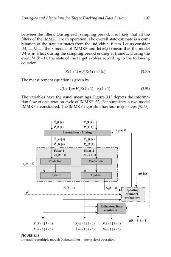
Strategies and Algorithms for Target Tracking and Data Fusion 107

between the fi lters. During each sampling period, it is likely that all the fi lters of the IMMKF are in operation. The overall state estimate is a com-bination of the state estimates from the individual fi lters. Let us consider

M1, ..., Mr as the r models of IMMKF and let Mj (k) mean that the model

Mj is in effect during the sampling period ending at frame k . During the event Mj (k + 1), the state of the target evolves according to the following equation

X(k + 1) = FjX(k) + wj (k) (3.90)

The measurement equation is given by

z(k + 1) = H jX(k + 1) + vj (k + 1) (3.91)

The variables have the usual meanings. Figure 3.13 depicts the informa-tion fl ow of one iteration-cycle of IMMKF [52]. For simplicity, a two-model IMMKF is considered. The IMMKF algorithm has four major steps [52,53].

FIGURE 3.13 Interactive multiple models Kalman fi lter—one cycle of operation.

X1(k|k)P1(k|k)

X2(k|k)

μi|j(k|k)

μ(k|k)

P2(k|k)

X01(k|k)

M1(k + 1) M2(k + 1)

P01(k|k)

X1(k + 1| k + 1)

P1(k + 1| k + 1)

X2(k + 1| k + 1)

P2(k + 1| k + 1)

X(k + 1| k + 1)μ(k + 1| k + 1)

Λ2(k + 1)Λ1(k + 1)

P(k + 1| k + 1)

X02(k|k)P02(k|k)

Filter-1 Filter-2

Interaction - Mixing

Prediction

Update

Prediction

Update

Updating of model

probability

Estimates/Statecombiner

pij

zm(k + 1)

108 Multi-Sensor Data Fusion: Theory and Practice

3.5.1.1 Interaction and Mixing

For the event Mj (k + 1) , the mixed estimate X0 j (k|k) and the covariance

matrix P0 j (k|k) are computed as

X0 j (k|k) = μ i|j (k|k)Xi (k|k)

i=1

r

∑

P0 j (k|k) = μ i|j (k|k) Pi (k|k) + Xi (k|k) − X

0 j (k|k)⎡⎣ ⎤⎦{i=1

r

∑ (3.92)

× Xi (k|k) − X

0 j (k|k)⎡⎣ ⎤⎦t }

The mixing probabilities μ i|j (k|k) are given by

μ i|j (k|k) = 1

μ j (k + 1|k)pijμ i (k|k) (3.93)

Here, the predicted mode probability μ j (k + 1|k) is computed by

μ j (k + 1|k) = pij

i=1

r

∑ μ i (k|k) (3.94)

The mode switching process is done by Markov process and is specifi ed by the following mode transition probabilities

pij = Pr Mj (k + 1)|Mi (k){ } (3.95)

Here, Pr{.} denotes the probability of an event, which means pij is the prob-ability at which Mi model at k th instant is switching over to Mj model at ( k + 1)th instant. This is used to calculate the model probabilities for the fi nal output.

3.5.1.2 Kalman Filtering

The usual KF equations are used with appropriate target motion models to update the mixed state estimates with current measurement as shown in Figure 3.13. The innovation covariance is given by

Sj = H j

%Pj (k + 1|k)H jT + Rj (3.96)

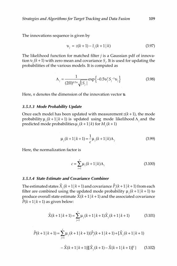
Strategies and Algorithms for Target Tracking and Data Fusion 109

The innovations sequence is given by

υ j = z(k + 1) − %zj (k + 1|k) (3.97)

The likelihood function for matched fi lter j is a Gaussian pdf of innova-tion υ j (k + 1) with zero mean and covariance Sj. It is used for updating the probabilities of the various models. It is computed as

Λ j = 1

(2Π)0.5n |Sj|exp −0.5υ j

TSj−1υ j{ } (3.98)

Here, n denotes the dimension of the innovation vector υ .

3.5.1.3 Mode Probability Update

Once each model has been updated with measurement z(k + 1), the mode probability μ j (k + 1|k + 1) is updated using mode likelihood Λ j and the predicted mode probabilities μ j (k + 1|k) for Mj (k + 1)

μ j (k + 1|k + 1) = 1

cμ j (k + 1|k)Λ j (3.99)

Here, the normalization factor is

c = μ i (k + 1|k)Λ i

i=1

r

∑ (3.100)

3.5.1.4 State Estimate and Covariance Combiner

The estimated states X j (k + 1|k + 1) and covariance Pj (k + 1|k + 1) from each fi lter are combined using the updated mode probability μ j (k + 1|k + 1) to

produce overall state estimate X(k + 1|k + 1) and the associated covariance

P(k + 1|k + 1) as given below:

X(k + 1|k + 1) = μ j

j=1

r

∑ (k + 1|k + 1)X j (k + 1|k + 1) (3.101)

P(k + 1|k + 1) = μ j

j=1

r

∑ (k + 1|k + 1){Pj (k + 1|k + 1) + [X j (k + 1|k + 1)

− X(k + 1|k + 1)][X j (k + 1) − X(k + 1|k + 1)]T } (3.102)

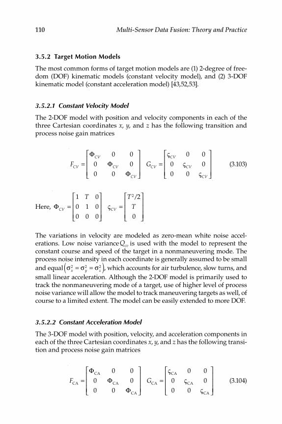
110 Multi-Sensor Data Fusion: Theory and Practice

3.5.2 Target Motion Models

The most common forms of target motion models are (1) 2-degree of free-dom (DOF) kinematic models (constant velocity model), and (2) 3-DOF kinematic model (constant acceleration model) [43,52,53].

3.5.2.1 Constant Velocity Model

The 2-DOF model with position and velocity components in each of the three Cartesian coordinates x , y , and z has the following transition and process noise gain matrices

FCV =ΦCV 0 0

0 ΦCV 0

0 0 ΦCV

⎡

⎣

⎢⎢⎢

⎤

⎦

⎥⎥⎥

GCV =ςCV 0 0

0 ςCV 0

0 0 ςCV

⎡

⎣

⎢⎢⎢

⎤

⎦

⎥⎥⎥

(3.103)

Here,

ΦCV =1 T 0

0 1 0

0 0 0

⎡

⎣

⎢⎢⎢

⎤

⎦

⎥⎥⎥

ςCV =T 2/2

T

0

⎡

⎣

⎢⎢⎢

⎤

⎦

⎥⎥⎥

The variations in velocity are modeled as zero-mean white noise accel-erations. Low noise variance Qcv is used with the model to represent the constant course and speed of the target in a nonmaneuvering mode. The process noise intensity in each coordinate is generally assumed to be small

and equal σx2 = σy

2 = σz2( ), which accounts for air turbulence, slow turns, and

small linear acceleration. Although the 2-DOF model is primarily used to track the nonmaneuvering mode of a target, use of higher level of process noise variance will allow the model to track maneuvering targets as well, of course to a limited extent. The model can be easily extended to more DOF.

3.5.2.2 Constant Acceleration Model

The 3-DOF model with position, velocity, and acceleration components in each of the three Cartesian coordinates x , y , and z has the following transi-tion and process noise gain matrices

FCA

=Φ

CA0 0

0 ΦCA

0

0 0 ΦCA

⎡

⎣

⎢⎢⎢

⎤

⎦

⎥⎥⎥

GCA=

ςCA

0 0

0 ςCA

0

0 0 ςCA

⎡

⎣

⎢⎢⎢

⎤

⎦

⎥⎥⎥

(3.104)

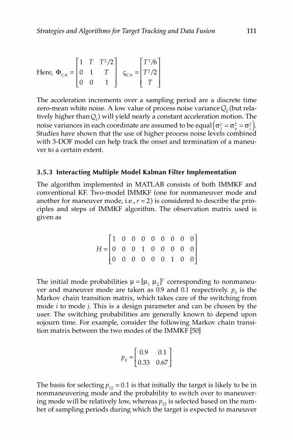
Strategies and Algorithms for Target Tracking and Data Fusion 111

Here,

ΦCA

=

1 T T 2/2

0 1 T

0 0 1

⎡

⎣

⎢⎢⎢

⎤

⎦

⎥⎥⎥

ςCA

=T 3/6

T 2/2

T

⎡

⎣

⎢⎢⎢

⎤

⎦

⎥⎥⎥

The acceleration increments over a sampling period are a discrete time zero-mean white noise. A low value of process noise variance Q2 (but rela-tively higher than Q

1) will yield nearly a constant acceleration motion. The

noise variances in each coordinate are assumed to be equal σx2 = σy

2 = σz2( ).

Studies have shown that the use of higher process noise levels combined with 3-DOF model can help track the onset and termination of a maneu-ver to a certain extent.

3.5.3 Interacting Multiple Model Kalman Filter Implementation

The algorithm implemented in MATLAB consists of both IMMKF and conventional KF. Two-model IMMKF (one for nonmaneuver mode and another for maneuver mode, i.e., r = 2) is considered to describe the prin-ciples and steps of IMMKF algorithm. The observation matrix used is given as

H =1 0 0 0 0 0 0 0 0

0 0 0 1 0 0 0 0 0

0 0 0 0 0 0 1 0 0

⎡

⎣

⎢⎢⎢

⎤

⎦

⎥⎥⎥

The initial mode probabilities μ = [μ1

μ2]T corresponding to nonmaneu-

ver and maneuver mode are taken as 0.9 and 0.1 respectively. pij is the Markov chain transition matrix, which takes care of the switching from mode i to mode j . This is a design parameter and can be chosen by the user. The switching probabilities are generally known to depend upon sojourn time. For example, consider the following Markov chain transi-tion matrix between the two modes of the IMMKF [50]

pij =

0.9 0.1

0.33 0.67

⎡

⎣⎢

⎤

⎦⎥

The basis for selecting p12

= 0.1 is that initially the target is likely to be in nonmaneuvering mode and the probability to switch over to maneuver-ing mode will be relatively low, whereas p

22 is selected based on the num-ber of sampling periods during which the target is expected to maneuver

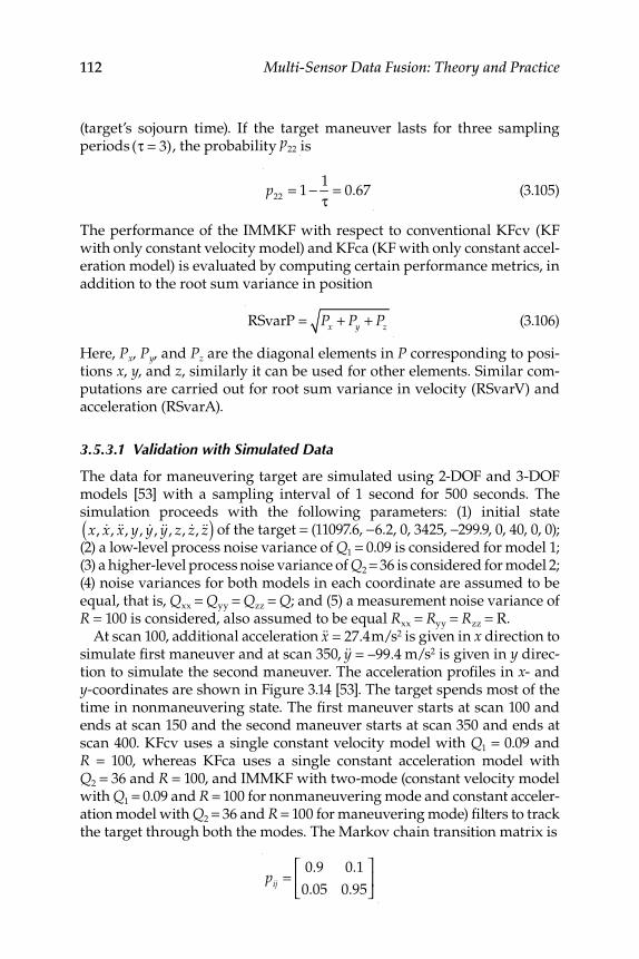
112 Multi-Sensor Data Fusion: Theory and Practice

(target’s sojourn time). If the target maneuver lasts for three sampling periods (τ = 3), the probability p22 is

p

22= 1 − 1

τ= 0.67 (3.105)

The performance of the IMMKF with respect to conventional KFcv (KF with only constant velocity model) and KFca (KF with only constant accel-eration model) is evaluated by computing certain performance metrics, in addition to the root sum variance in position

RSvarP = Px + Py + Pz (3.106)

Here, Px, Py, and Pz are the diagonal elements in P corresponding to posi-tions x , y , and z , similarly it can be used for other elements. Similar com-putations are carried out for root sum variance in velocity (RSvarV) and acceleration (RSvarA).

3.5.3.1 Validation with Simulated Data

The data for maneuvering target are simulated using 2-DOF and 3-DOF models [53] with a sampling interval of 1 second for 500 seconds. The simulation proceeds with the following parameters: (1) initial state

x, &x, &&x, y, &y, &&y, z, &z, &&z( ) of the target = (11097.6, −6.2, 0, 3425, −299.9, 0, 40, 0, 0); (2) a low-level process noise variance of Q 1 = 0.09 is considered for model 1; (3) a higher-level process noise variance of Q 2 = 36 is considered for model 2; (4) noise variances for both models in each coordinate are assumed to be equal, that is, Qxx = Qyy = Qzz = Q; and (5) a measurement noise variance of R = 100 is considered, also assumed to be equal Rxx = Ryy = Rzz = R.

At scan 100, additional acceleration &&x = 27.4m/s 2 is given in x direction to simulate fi rst maneuver and at scan 350, &&y = −99.4 m/s 2 is given in y direc-tion to simulate the second maneuver. The acceleration profi les in x - and y -coordinates are shown in Figure 3.14 [53]. The target spends most of the time in nonmaneuvering state. The fi rst maneuver starts at scan 100 and ends at scan 150 and the second maneuver starts at scan 350 and ends at scan 400. KFcv uses a single constant velocity model with Q 1 = 0.09 and R = 100, whereas KFca uses a single constant acceleration model with Q 2 = 36 and R = 100, and IMMKF with two-mode (constant velocity model with Q 1 = 0.09 and R = 100 for nonmaneuvering mode and constant acceler-ation model with Q 2 = 36 and R = 100 for maneuvering mode) fi lters to track the target through both the modes. The Markov chain transition matrix is

pij =

0.9 0.1

0.05 0.95

⎡

⎣⎢

⎤

⎦⎥

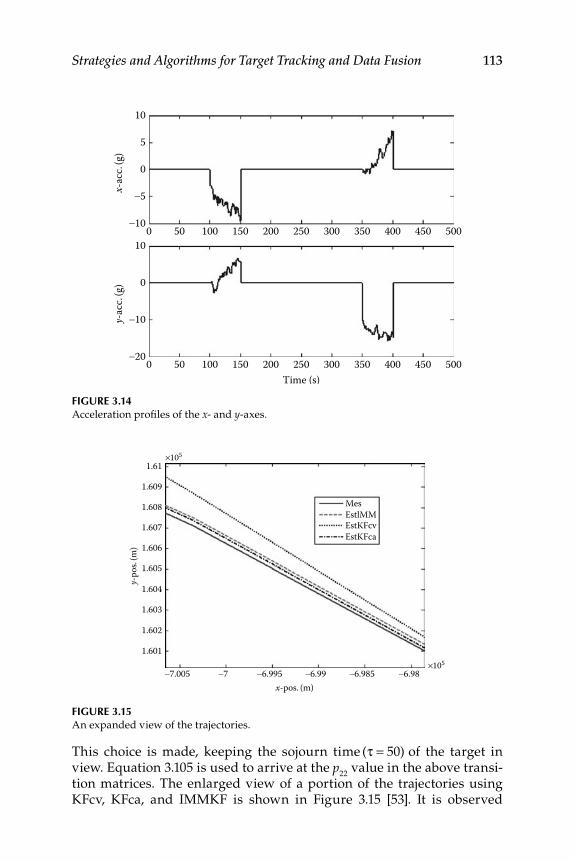
Strategies and Algorithms for Target Tracking and Data Fusion 113

This choice is made, keeping the sojourn time (τ = 50) of the target in view. Equation 3.105 is used to arrive at the p

22value in the above transi-

tion matrices. The enlarged view of a portion of the trajectories using KFcv, KFca, and IMMKF is shown in Figure 3.15 [53]. It is observed

FIGURE 3.14 Acceleration profi les of the x - and y -axes.

10

5

0

-5x-ac

c.(g

)

-100 50 100 150 200 250 300 350 400 450 500

10

0

-10y-ac

c.(g

)

-200 50 100 150 200 250

Time (s)300 350 400 450 500

FIGURE 3.15 An expanded view of the trajectories.

1.61

1.609

1.608

1.607

1.606

y-po

s.(m

)

x-pos. (m)

×105

×105

1.605

1.604

1.603

1.602

1.601

-7.005 -7 -6.995 -6.99 -6.985 -6.98

MesEstlMMEstKFcvEstKFca

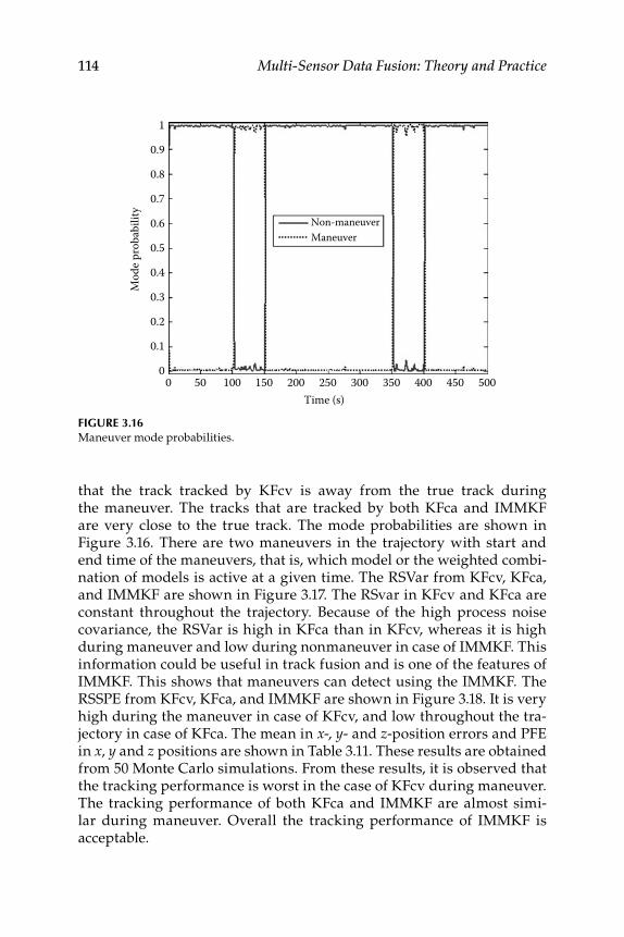
114 Multi-Sensor Data Fusion: Theory and Practice

that the track tracked by KFcv is away from the true track during the maneuver. The tracks that are tracked by both KFca and IMMKF are very close to the true track. The mode probabilities are shown in Figure 3.16. There are two maneuvers in the trajectory with start and end time of the maneuvers, that is, which model or the weighted combi-nation of models is active at a given time. The RSVar from KFcv, KFca, and IMMKF are shown in Figure 3.17. The RSvar in KFcv and KFca are constant throughout the trajectory. Because of the high process noise covariance, the RSVar is high in KFca than in KFcv, whereas it is high during maneuver and low during nonmaneuver in case of IMMKF. This information could be useful in track fusion and is one of the features of IMMKF. This shows that maneuvers can detect using the IMMKF. The RSSPE from KFcv, KFca, and IMMKF are shown in Figure 3.18. It is very high during the maneuver in case of KFcv, and low throughout the tra-jectory in case of KFca. The mean in x -, y - and z -position errors and PFE in x , y and z positions are shown in Table 3.11. These results are obtained from 50 Monte Carlo simulations. From these results, it is observed that the tracking performance is worst in the case of KFcv during maneuver. The tracking performance of both KFca and IMMKF are almost simi-lar during maneuver. Overall the tracking performance of IMMKF is acceptable.

FIGURE 3.16 Maneuver mode probabilities.

1

0.9

0.8

0.7

0.6

0.5

Mod

e pro

babi

lity

0.4

0.3

0.2

0.1

0 50 100 150 200 250Time (s)

Non-maneuverManeuver

350300 400 450 5000

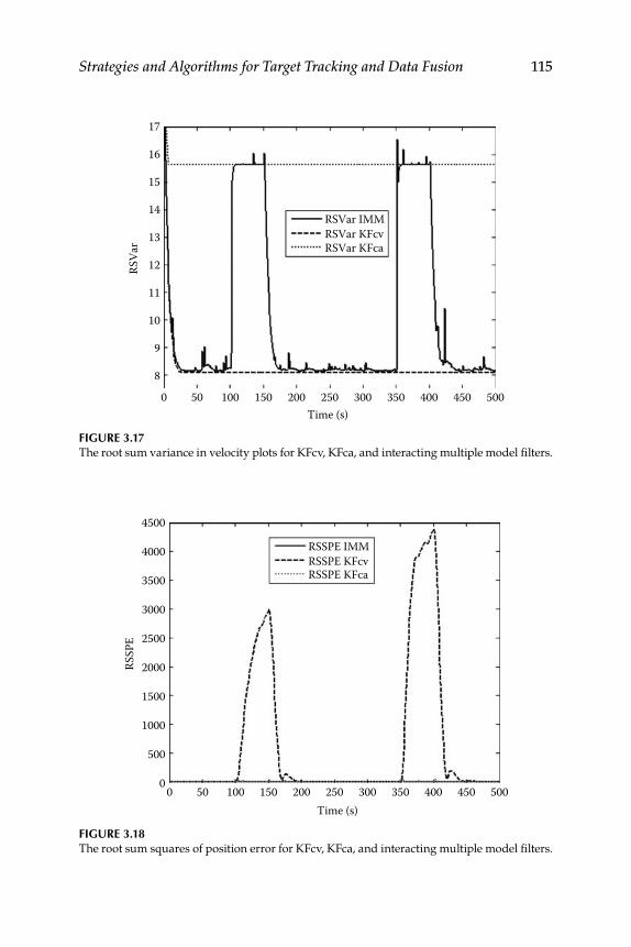
Strategies and Algorithms for Target Tracking and Data Fusion 115

FIGURE 3.18 The root sum squares of position error for KFcv, KFca, and interacting multiple model fi lters.

4500

RSSPE IMM

RSSP

E

RSSPE KFcvRSSPE KFca

4000

3500

3000

2500

2000

1500

1000

500

0

Time (s)0 50 100 150 200 250 300 350 400 450 500

FIGURE 3.17 The root sum variance in velocity plots for KFcv, KFca, and interacting multiple model fi lters.

RSVar IMM

17

16

15

14

13

12RSVa

r

11

10

9

8

RSVar KFcvRSVar KFca

0 50 100 150 200 250Time (s)

300 350 400 450 500

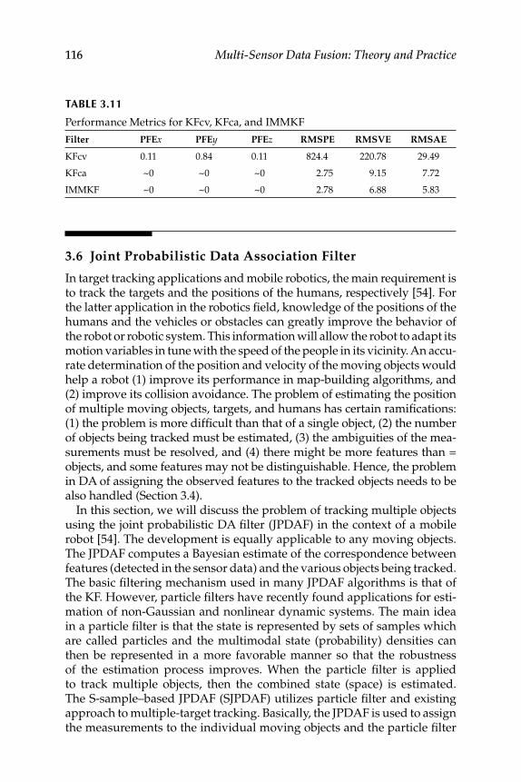
116 Multi-Sensor Data Fusion: Theory and Practice

3.6 Joint Probabilistic Data Association Filter

In target tracking applications and mobile robotics, the main requirement is to track the targets and the positions of the humans, respectively [54]. For the latter application in the robotics fi eld, knowledge of the positions of the humans and the vehicles or obstacles can greatly improve the behavior of the robot or robotic system. This information will allow the robot to adapt its motion variables in tune with the speed of the people in its vicinity. An accu-rate determination of the position and velocity of the moving objects would help a robot (1) improve its performance in map-building algorithms, and (2) improve its collision avoidance. The problem of estimating the position of multiple moving objects, targets, and humans has certain ramifi cations: (1) the problem is more diffi cult than that of a single object, (2) the number of objects being tracked must be estimated, (3) the ambiguities of the mea-surements must be resolved, and (4) there might be more features than = objects, and some features may not be distinguishable. Hence, the problem in DA of assigning the observed features to the tracked objects needs to be also handled (Section 3.4).

In this section, we will discuss the problem of tracking multiple objects using the joint probabilistic DA fi lter (JPDAF) in the context of a mobile robot [54]. The development is equally applicable to any moving objects. The JPDAF computes a Bayesian estimate of the correspondence between features (detected in the sensor data) and the various objects being tracked. The basic fi ltering mechanism used in many JPDAF algorithms is that of the KF. However, particle fi lters have recently found applications for esti-mation of non-Gaussian and nonlinear dynamic systems. The main idea in a particle fi lter is that the state is represented by sets of samples which are called particles and the multimodal state (probability) densities can then be represented in a more favorable manner so that the robustness of the estimation process improves. When the particle fi lter is applied to track multiple objects, then the combined state (space) is estimated. The S-sample–based JPDAF (SJPDAF) utilizes particle fi lter and existing approach to multiple-target tracking. Basically, the JPDAF is used to assign the measurements to the individual moving objects and the particle fi lter

TABLE 3.11

Performance Metrics for KFcv, KFca, and IMMKF

Filter PFEx PFEy PFEz RMSPE RMSVE RMSAE

KFcv 0.11 0.84 0.11 824.4 220.78 29.49

KFca ~0 ~0 ~0 2.75 9.15 7.72

IMMKF ~0 ~0 ~0 2.78 6.88 5.83

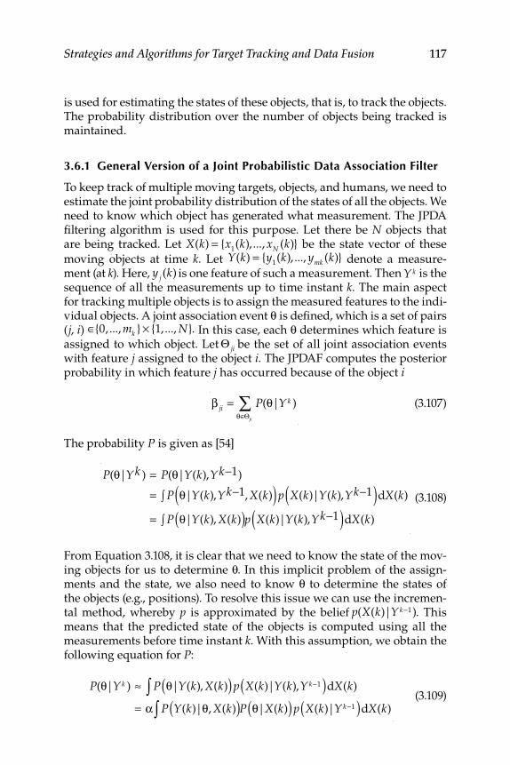
Strategies and Algorithms for Target Tracking and Data Fusion 117

is used for estimating the states of these objects, that is, to track the objects. The probability distribution over the number of objects being tracked is maintained.

3.6.1 General Version of a Joint Probabilistic Data Association Filter

To keep track of multiple moving targets, objects, and humans, we need to estimate the joint probability distribution of the states of all the objects. We need to know which object has generated what measurement. The JPDA fi ltering algorithm is used for this purpose. Let there be N objects that are being tracked. Let X(k) = {x

1(k), ..., xN (k)} be the state vector of these

moving objects at time k . Let Y(k) = {y1(k), ..., ymk (k)} denote a measure-

ment (at k ). Here, yj (k) is one feature of such a measurement. Then Yk is the sequence of all the measurements up to time instant k . The main aspect for tracking multiple objects is to assign the measured features to the indi-vidual objects. A joint association event θ is defi ned, which is a set of pairs ( j , i ) ∈{0, ..., mk } × {1, ..., N}. In this case, each θ determines which feature is assigned to which object. Let Θ ji be the set of all joint association events with feature j assigned to the object i . The JPDAF computes the posterior probability in which feature j has occurred because of the object i

β ji = P(θ|Yk

θ∈Θji

∑ ) (3.107)

The probability P is given as [54]

P(θ|Yk ) = P(θ|Y(k),Yk−1)

= P θ|Y(k),Yk−1, X(k)( ) p X(k)|Y(k),Yk−1( )dX(k)∫

= P θ|Y(k), X(k)( )∫ p X(k)|Y(k),Yk−1( )dX(k)

(3.108)

From Equation 3.108, it is clear that we need to know the state of the mov-ing objects for us to determine θ. In this implicit problem of the assign-ments and the state, we also need to know θ to determine the states of the objects (e.g., positions). To resolve this issue we can use the incremen-tal method, whereby p is approximated by the belief p(X(k)|Yk−1). This means that the predicted state of the objects is computed using all the measurements before time instant k . With this assumption, we obtain the following equation for P:

P(θ|Yk ) ≈ P θ|Y(k), X(k)( ) p X(k)|Y(k),Yk−1( )dX(k)∫= α P Y(k)|θ, X(k)( )∫ P θ|X(k)( ) p X(k)|Yk−1( )dX(k)

(3.109)

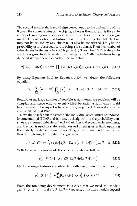
118 Multi-Sensor Data Fusion: Theory and Practice

The second term in the integral sign corresponds to the probability of the θ given the current states of the objects, whereas the fi rst term is the prob-ability of making an observation given the states and a specifi c assign-ment between the observed features and the tracked objects. That a feature may not be caused by any object must also be considered. Let γ be the probability of an observed feature being a false alarm. Then the number of false alarms in the association θ is (mk −|θ|). Thus, the γ (mk −|θ|) is the prob-ability assigned to all false alarms in Y ( k ) given θ. With the features being detected independently of each other, we obtain

P Y(k)|θ, X(k)( ) = γ (mk −|θ|) p zj (k)|xi (k)( ) p xi (k)|Yk−1( )dxi (k)∫( j,i)∈θ∏ (3.110)

By using Equation 3.110 in Equation 3.109, we obtain the following equation:

β ji = αγ (mk −|θ|)⎡⎣ ⎤⎦θ∈Θ ji

∑ p zj (k)|xi (k)( ) p xi (k)|Yk−1( )dxi (k)∫( j ,i)∈θ∏ (3.111)

Because of the large number of possible assignments, the problem will be complex and hence only an event with substantial assignments should be considered. This aspect is handled by gating and DA, as is done in the case of NNKF and PDAF.

Next, the belief about the states of the individual objects must be updated. In conventional JPDAF and in many such algorithms, the probability den-sities are assumed to be described by their fi rst and second order moments, and then KF is used for state prediction and fi ltering (essentially updating the underlying densities via the updating of the moments). In case of the Bayesian fi ltering, this updating is given as

p xi (k)|Yk−1( ) = p xi (k)|xi (k − 1), t( ) p xi (k − 1)|Yk−1( )dxi (k − 1)∫ (3.112)

With the new measurements the state is updated as follows:

p xi (k)|Yk( ) = α p Z(k)|xi (k)( ) p xi (k)|Yk−1( ) (3.113)

Next, the single features are integrated with assignment probabilities β ji

p xi (k)|Yk( ) = α β ji p zj (k)|xi (k)( ) p xi (k)|Yk−1( )

j=0

mk

∑ (3.114)

From the foregoing development it is clear that we need the models p(xi (k)|Xi (k − 1), t) and p(zi (k)|xi (k)). We can see that these models depend

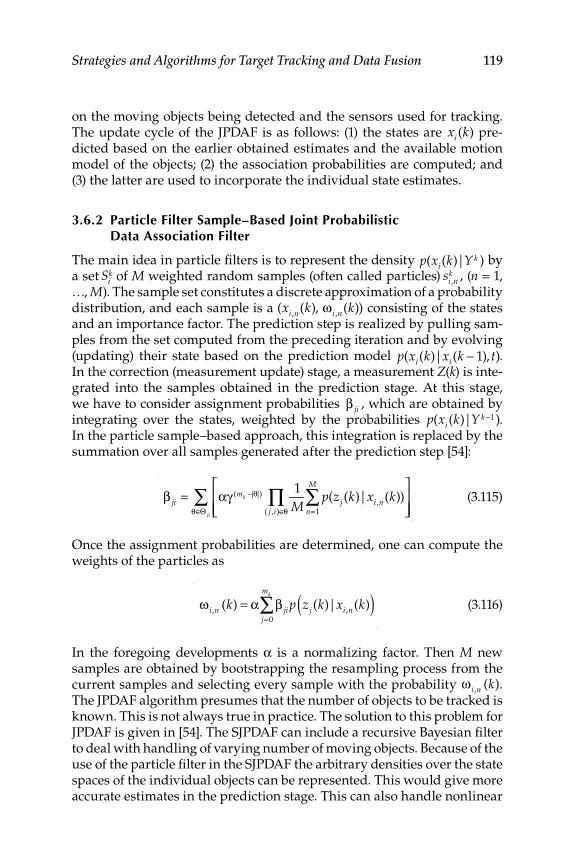
Strategies and Algorithms for Target Tracking and Data Fusion 119

on the moving objects being detected and the sensors used for tracking. The update cycle of the JPDAF is as follows: (1) the states are xi (k) pre-dicted based on the earlier obtained estimates and the available motion model of the objects; (2) the association probabilities are computed; and (3) the latter are used to incorporate the individual state estimates.

3.6.2 Particle Filter Sample–Based Joint Probabilistic Data Association Filter

The main idea in particle fi lters is to represent the density p(xi (k)|Yk ) by a set Si

k of M weighted random samples (often called particles) si ,nk , ( n = 1,

…, M ). The sample set constitutes a discrete approximation of a probability distribution, and each sample is a (xi ,n(k), ω i ,n(k)) consisting of the states and an importance factor. The prediction step is realized by pulling sam-ples from the set computed from the preceding iteration and by evolving (updating) their state based on the prediction model p(xi (k)|xi (k − 1), t). In the correction (measurement update) stage, a measurement Z ( k ) is inte-grated into the samples obtained in the prediction stage. At this stage, we have to consider assignment probabilities β ji , which are obtained by integrating over the states, weighted by the probabilities p(xi (k)|Yk−1). In the particle sample–based approach, this integration is replaced by the summation over all samples generated after the prediction step [54]:

β ji = αγ (mk −|θ|)1

M( j ,i)∈θ∏ p(zj (k)|xi ,n(k))

n=1

M

∑⎡

⎣⎢⎢

⎤

⎦⎥⎥θ∈Θ ji

∑ (3.115)

Once the assignment probabilities are determined, one can compute the weights of the particles as

ω i ,n (k) = α β ji p zj (k)|xi ,n(k)( )

j=0

mk

∑ (3.116)

In the foregoing developments α is a normalizing factor. Then M new samples are obtained by bootstrapping the resampling process from the current samples and selecting every sample with the probability ω i ,n (k). The JPDAF algorithm presumes that the number of objects to be tracked is known. This is not always true in practice. The solution to this problem for JPDAF is given in [54]. The SJPDAF can include a recursive Bayesian fi lter to deal with handling of varying number of moving objects. Because of the use of the particle fi lter in the SJPDAF the arbitrary densities over the state spaces of the individual objects can be represented. This would give more accurate estimates in the prediction stage. This can also handle nonlinear

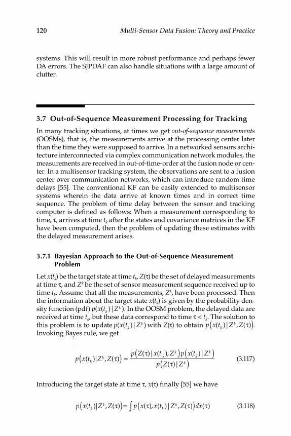
120 Multi-Sensor Data Fusion: Theory and Practice

systems. This will result in more robust performance and perhaps fewer DA errors. The SJPDAF can also handle situations with a large amount of clutter.

3.7 Out-of-Sequence Measurement Processing for Tracking

In many tracking situations, at times we get out-of-sequence measurements (OOSMs), that is, the measurements arrive at the processing center later than the time they were supposed to arrive. In a networked sensors archi-tecture interconnected via complex communication network modules, the measurements are received in out-of-time-order at the fusion node or cen-ter. In a multisensor tracking system, the observations are sent to a fusion center over communication networks, which can introduce random time delays [55]. The conventional KF can be easily extended to multisensor systems wherein the data arrive at known times and in correct time sequence. The problem of time delay between the sensor and tracking computer is defi ned as follows: When a measurement corresponding to time, τ, arrives at time t k after the states and covariance matrices in the KF have been computed, then the problem of updating these estimates with the delayed measurement arises.

3.7.1 Bayesian Approach to the Out-of-Sequence Measurement Problem

Let x ( t k ) be the target state at time t k , Z (τ) be the set of delayed measurements at time τ, and Z k be the set of sensor measurement sequence received up to time t k . Assume that all the measurements, Z k , have been processed. Then the information about the target state x ( t k ) is given by the probability den-sity function (pdf) p(x(tk )|Zk ). In the OOSM problem, the delayed data are received at time t k , but these data correspond to time τ < t k . The solution to this problem is to update p(x(tk )|Zk ) with Z (τ) to obtain p x(tk )|Zk , Z(τ)( ). Invoking Bayes rule, we get

p x(tk )|Zk , Z(τ)( ) = p Z(τ)|x(t k ), Zk( ) p x(tk )|Zk( )

p Z(τ)|Zk( ) (3.117)

Introducing the target state at time τ, x (τ) fi nally [55] we have

p x(tk )|Zk , Z(τ)( )= p x(τ), x(tk )|Zk , Z(τ)( )dx(τ)∫ (3.118)

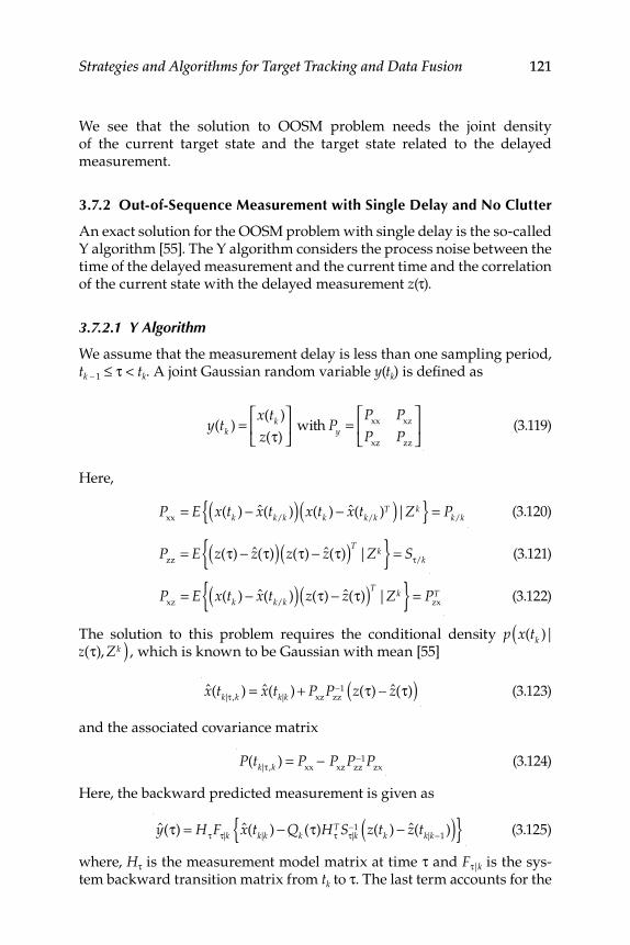
Strategies and Algorithms for Target Tracking and Data Fusion 121

We see that the solution to OOSM problem needs the joint density of the current target state and the target state related to the delayed measurement.

3.7.2 Out-of-Sequence Measurement with Single Delay and No Clutter

An exact solution for the OOSM problem with single delay is the so-called Y algorithm [55]. The Y algorithm considers the process noise between the time of the delayed measurement and the current time and the correlation of the current state with the delayed measurement z (τ).

3.7.2.1 Y Algorithm

We assume that the measurement delay is less than one sampling period, t k − 1 ≤ τ < t k . A joint Gaussian random variable y ( t k ) is defi ned as

y(tk ) =x(tk )

z(τ)

⎡

⎣⎢

⎤

⎦⎥ with Py =

Pxx

Pxz

Pxz

Pzz

⎡

⎣⎢

⎤

⎦⎥ (3.119)

Here,

Pxx

= E x(tk ) − x(tk/k )( ) x(tk ) − x(tk/k )T( )|Zk{ } = Pk/k (3.120)

Pzz

= E z(τ) − z(τ)( ) z(τ) − z(τ)( )T|Zk{ } = Sτ/k (3.121)

Pxz

= E x(tk ) − x(tk/k )( ) z(τ) − z(τ)( )T|Zk{ } = P

zxT (3.122)

The solution to this problem requires the conditional density p x(tk )|(z(τ), Zk ) , which is known to be Gaussian with mean [55]

x(tk|τ ,k ) = x(tk|k ) + P

xzP

zz−1 z(τ) − z(τ)( ) (3.123)

and the associated covariance matrix

P(tk|τ ,k ) = P

xx− P

xzP

zz−1P

zx (3.124)

Here, the backward predicted measurement is given as

y(τ) = HτFτ|k x(tk|k ) − Qk (τ)Hτ

TSτ|k−1 z(tk ) − z(tk|k−1

)( ){ } (3.125)

where, H τ is the measurement model matrix at time τ and F τ| k is the sys-tem backward transition matrix from t k to τ. The last term accounts for the

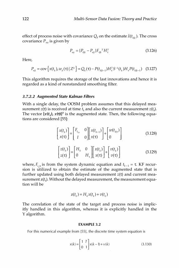
122 Multi-Sensor Data Fusion: Theory and Practice

effect of process noise with covariance Q k on the estimate x(tk|k ). The cross covariance P xz is given by

P

xz= {Pk|k − P

x%z }Fτ|kT Hτ

T (3.126)

Here,

Px%z = cov x(tk ), wk (τ)|Zk{ } = Qk (τ) − P(tk|k−1

)HτTS−1(tk )HτP(tk|k−1

) (3.127)

This algorithm requires the storage of the last innovations and hence it is regarded as a kind of nonstandard smoothing fi lter.

3.7.2.2 Augmented State Kalman Filters

With a single delay, the OOSM problem assumes that this delayed mea-surement z (τ) is received at time t k and also the current measurement z ( t k ). The vector [x(t k ), x(τ)] T is the augmented state. Then, the following equa-tions are considered [55]:

x(tk )

x(τ)

⎡

⎣⎢

⎤

⎦⎥ =

Ftk|τ0

I 0

⎡

⎣⎢⎢

⎤

⎦⎥⎥

x(tk−1)

x(τ)

⎡

⎣⎢

⎤

⎦⎥ +

w(tk|τ )

0

⎡

⎣⎢⎢

⎤

⎦⎥⎥

(3.128)

z(tk )

z(τ)

⎡

⎣⎢

⎤

⎦⎥ =

Hk 0

0 Hτ

⎡

⎣⎢

⎤

⎦⎥

x(tk )

x(τ)

⎡

⎣⎢

⎤

⎦⎥ +

v(tk )

v(τ)

⎡

⎣⎢

⎤

⎦⎥ (3.129)

where, Ftk|τ is from the system dynamic equation and t k − 1 = τ. KF recur-sion is utilized to obtain the estimate of the augmented state that is further updated using both delayed measurement z (τ) and current mea-surement z( t k ). Without the delayed measurement, the measurement equa-tion will be

z(tk ) = Hk x(tk ) + v(tk )

The correlation of the state of the target and process noise is implic-itly handled in this algorithm, whereas it is explicitly handled in the Y algorithm.

EXAMPLE 3.2

For this numerical example from [55], the discrete time system equation is

x(k) =

1 T

0 1

⎡

⎣⎢

⎤

⎦⎥ x(k −1)+ v(k) (3.130)

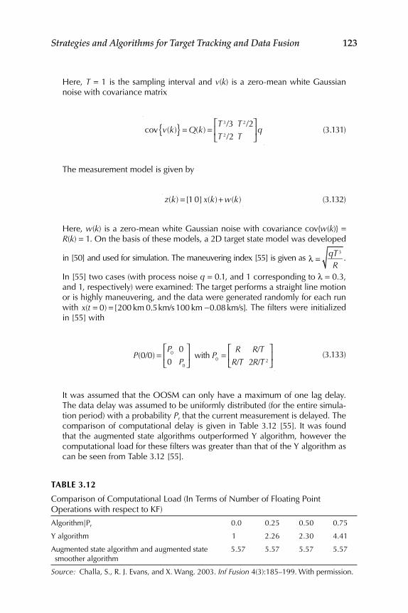
Strategies and Algorithms for Target Tracking and Data Fusion 123

Here, T = 1 is the sampling interval and v ( k ) is a zero-mean white Gaussian noise with covariance matrix

cov v(k){ } = Q(k) =

T 3/3 T 2/2

T 2/2 T

⎡

⎣⎢

⎤

⎦⎥q (3.131)

The measurement model is given by

z(k) = [1 0] x(k)+ w(k) (3.132)

Here, w ( k ) is a zero-mean white Gaussian noise with covariance cov{ w ( k )} = R ( k ) = 1. On the basis of these models, a 2D target state model was developed

in [50] and used for simulation. The maneuvering index [55] is given as λ = qT 3

R.

In [55] two cases (with process noise q = 0.1, and 1 corresponding to λ = 0.3, and 1, respectively) were examined: The target performs a straight line motion or is highly maneuvering, and the data were generated randomly for each run with x(t = 0) = [200 km 0.5km/s100 km −0.08km/s]. The fi lters were initialized in [55] with

P(0/0) =P0 0

0 P0

⎡

⎣⎢

⎤

⎦⎥ with P0 =

R R/T

R/T 2R/T 2

⎡

⎣⎢

⎤

⎦⎥ (3.133)

It was assumed that the OOSM can only have a maximum of one lag delay. The data delay was assumed to be uniformly distributed (for the entire simula-tion period) with a probability P r that the current measurement is delayed. The comparison of computational delay is given in Table 3.12 [55]. It was found that the augmented state algorithms outperformed Y algorithm, however the computational load for these fi lters was greater than that of the Y algorithm as can be seen from Table 3.12 [55].

TABLE 3.12

Comparison of Computational Load (In Terms of Number of Floating Point Operations with respect to KF)

Algorithm|Pr 0.0 0.25 0.50 0.75

Y algorithm 1 2.26 2.30 4.41

Augmented state algorithm and augmented state smoother algorithm

5.57 5.57 5.57 5.57

Source: Challa, S., R. J. Evans, and X. Wang. 2003. Inf Fusion 4(3):185–199. With permission.

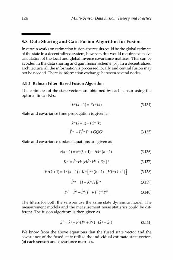
124 Multi-Sensor Data Fusion: Theory and Practice

3.8 Data Sharing and Gain Fusion Algorithm for Fusion

In certain works on estimation fusion, the results could be the global estimate of the state in a decentralized system; however, this would require extensive calculation of the local and global inverse covariance matrices. This can be avoided in the data sharing and gain fusion scheme [56]. In a decentralized architecture, all the information is processed locally and central fusion may not be needed. There is information exchange between several nodes.

3.8.1 Kalman Filter–Based Fusion Algorithm

The estimates of the state vectors are obtained by each sensor using the optimal linear KFs:

%xm(k + 1) = Fxm(k) (3.134)

State and covariance time propagation is given as

%xm(k + 1)= Fxm(k)

%Pm = FPmFt + GQGt (3.135)

State and covariance update equations are given as

r(k + 1) = zm(k + 1) − H%xm(k + 1) (3.136)

Km = %PmHt[H %PmHt + Rv

m ]−1 (3.137)

xm(k + 1) = %xm(k + 1) + Km zm(k + 1) − H%xm(k + 1)⎡⎣ ⎤⎦ (3.138)

Pm = [I − KmH] %Pm (3.139)

P

f = P1 − P1(P1 + P2 )−1 P1t (3.140)

The fi lters for both the sensors use the same state dynamics model. The measurement models and the measurement noise statistics could be dif-ferent. The fusion algorithm is then given as

x

f = x1 + P1(P1 + P2 )−1(x2 − x1) (3.141)

We know from the above equations that the fused state vector and the covariance of the fused state utilize the individual estimate state vectors (of each sensor) and covariance matrices.

Strategies and Algorithms for Target Tracking and Data Fusion 125

3.8.2 Gain Fusion–Based Algorithm

We know from the equations in Section 3.8.1 that the KF-based fusion algorithm (KFBFA) requires calculations of inverse covariance to obtain the global results, Equations 3.140 and 3.141. The recent fusion algorithm [56] does not require calculations of covariance inverses and has parallel processing capability. The dynamic system equations are the same as also used in KF equations. The gain fusion algorithm for multisensor integra-tion involves information feedback from the global fi lter to the local fi l-ters. The fi ltering algorithm is given next [56].

Time propagation of global estimates is

%xf (k + 1) = Fx f (k) (3.142)

%P f (k + 1) = FP f (k)Ft + GQGt (3.143)

The local fi lters are reset as

%xm(k + 1) = %x f (k + 1) (3.144)

%Pm(k + 1) = %P f (k + 1) (3.145)

The measurement update of local gains and states is obtained by

Km = 1/γ m( ) %P f k + 1( ) ′H H %P f k + 1( ) ′H + 1/γ m( )Rm⎡⎣ ⎤⎦

−1

(3.146)

xm k + 1( ) = %x f k + 1( ) + km zm k + 1( ) − H%x f k + 1( )⎡⎣ ⎤⎦ (3.147)

The global fusion of m local estimates is given as

x f (k + 1) = xm(k + 1) − (m − 1) %x f (k + 1)

m

∑ (3.148)

P f (k + 1) = I − KmHm

∑⎡

⎣⎢

⎤

⎦⎥ %P f (k + 1) I − KmH

m

∑⎡

⎣⎢

⎤

⎦⎥

t

+ KmRmKmtm

∑ (3.149)

We see that there is information feedback from the global fi lter to the local fi lters. The GFBA does not need the measurement update of the local cova-riances to obtain the global estimates. Because the global a priori estimates are fed back to the local fi lter, there is implicit measurement data sharing between the local fi lters [56]. This feature is evaluated when there is data loss in either of the two sensors.

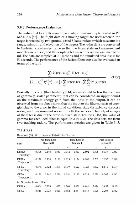
126 Multi-Sensor Data Fusion: Theory and Practice

3.8.3 Performance Evaluation

The individual local fi lters and fusion algorithms are implemented in PC MATLAB [57]. The fl ight data of a moving target are used wherein the target is tracked by two ground-based S-band radars (which measure the range, azimuth, and elevation of the target). The radar data are converted to Cartesian coordinates frame so that the linear state and measurement models can be used, and the coupling between three axes is assumed to be nil. The data are sampled at 0.1 seconds and the simulated data loss is for 50 seconds. The performance of the fusion fi lters can also be evaluated in terms of the ratio

x f (k) − x(k)( )tx f (k) − x(k)( )

k=0

N

∑

x0

f − x0

f( )tP

0

f x0

f − x0

f( ) + wt (k)w(k) + vmt (k)vm(k)k=0

N

∑m

∑k=0

N

∑ (3.150)

Basically this ratio (the H-infi nity [H-I] norm) should be less than square of gamma (a scalar parameter) that can be considered an upper bound on the maximum energy gain from the input to the output. It can be observed from the above norm that the input to the fi lter consists of ener-gies due to the error in the initial condition, state disturbance (process noise), and measurement noise for both the sensors. The output energy of the fi lter is due to the error in fused state. For the GFBA, the value of gamma for each local fi lter is equal to 2 ( m = 2). The data sets are from two tracking radars. The performance metrics are given in Table 3.13.

TABLE 3.13

Residual (%) Fit Errors and H-Infi nity Norms

PFE

No Data Loss

(Normal)

Data Loss in

Sensor 1

Data Loss in

Sensor 2

x y z x y z x y z

KFBFA

Trajectory 1

0.308 0.140 0.553 1.144 1.543 2.802 0.308 0.139 0.553

KFBFA

Trajectory 2

0.129 0.124 0.180 0.129 0.124 0.180 0.762 1.157 6.199

GFBA

Trajectory 1

0.376 0.622 1.306 0.379 0.627 1.328 0.392 0.610 1.604

GFBA

Trajectory 2

0.131 0.142 0.226 0.131 0.142 0.219 0.220 0.205 1.142

H∞ Norm for fusion fi lters

KFBFA 0.604 2.759 1.037 0.704 3.051 0.941 5.076 19.55 69.85

GFBA 0.546 2.325 0.821 0.562 2.38 0.913 0.625 2.203 2.952

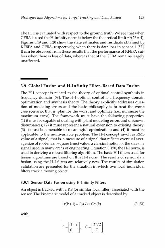
Strategies and Algorithms for Target Tracking and Data Fusion 127

The PFE is evaluated with respect to the ground truth. We see that when GFBA is used the H-infi nity norm is below the theoretical limit γ m(22 = 4). Figures 3.19 and 3.20 show the state estimates and residuals obtained by KFBFA and GFBA, respectively, when there is data loss in sensor 1 [57]. It can be observed from these results that the performance of KFBFA suf-fers when there is loss of data, whereas that of the GFBA remains largely unaffected.

3.9 Global Fusion and H-Infinity Filter–Based Data Fusion

The H-I concept is related to the theory of optimal control synthesis in frequency domain [58]. The H-I optimal control is a frequency domain optimization and synthesis theory. The theory explicitly addresses ques-tion of modeling errors and the basic philosophy is to treat the worst case scenario, that is, plan for the worst and optimize (i.e., minimize the maximum error). The framework must have the following properties: (1) it must be capable of dealing with plant modeling errors and unknown disturbances; (2) it must represent a natural extension to existing theory; (3) it must be amenable to meaningful optimization; and (4) it must be applicable to the multivariable problem. The H-I concept involves RMS value of a signal, that is, a measure of a signal that refl ects eventual aver-age size of root-mean-square (rms) value, a classical notion of the size of a signal used in many areas of engineering. Equation 3.150, the H-I norm, is used in deriving a robust fi ltering algorithm. The basic H-I fi lters used for fusion algorithms are based on this H-I norm. The results of sensor data fusion using the H-I fi lters are relatively new. The results of simulation validation are presented for the situation in which two local individual fi lters track a moving object.

3.9.1 Sensor Data Fusion using H-Infinity Filters

An object is tracked with a KF (or similar local fi lter) associated with the sensor. The kinematic model of a tracked object is described by

x(k + 1) = Fx(k) + Gw(k) (3.151)

with

F =

1 T

0 1

⎡

⎣⎢

⎤

⎦⎥ ; G =

T 2/2

T

⎡

⎣⎢

⎤

⎦⎥

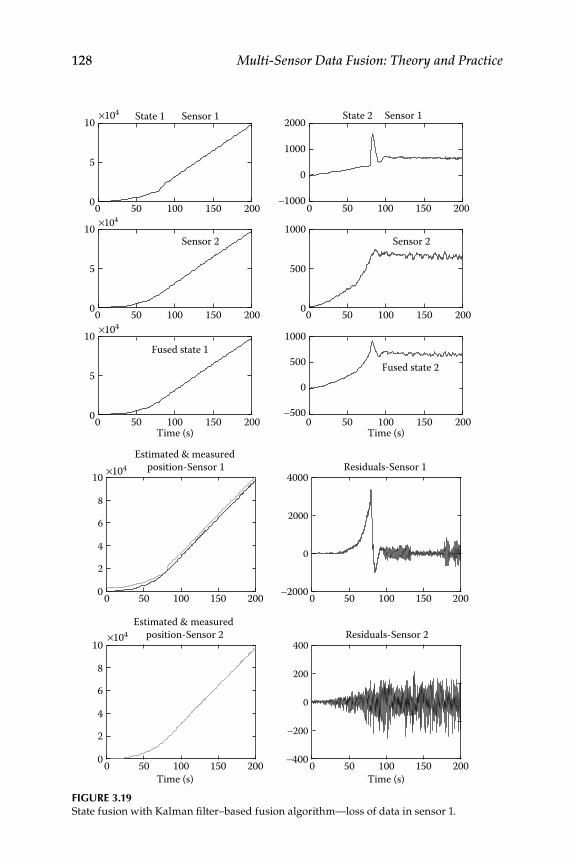
128 Multi-Sensor Data Fusion: Theory and Practice

0

2

4

6

8

10

0 50 100 150 2000

5

10 ×104

×104

State 1 Sensor 1

0 50 100 150 200-1000

0

1000

2000 State 2 Sensor 1

Time (s)Time (s)

0 50 100 150 200

Fused state 2Fused state 1

Estimated & measured position-Sensor 1

0 50 100 150 2000

5

10Sensor 2

0 50 100 150 2000

500

1000Sensor 2

×104

×104

0 50 100 150 2000

4000

0 50 100 150 200-2000

0

2000

Residuals-Sensor 1

0

2

4

6

8

10

0 50 100 150 200

Estimated & measured position-Sensor 2×104

400

0 50 100 150 200-400

0

200

Residuals-Sensor 2

-200

5

10

0 50 100 150 200

500

-500

0

1000

Time (s) Time (s) FIGURE 3.19 State fusion with Kalman fi lter–based fusion algorithm—loss of data in sensor 1.

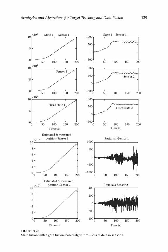
Strategies and Algorithms for Target Tracking and Data Fusion 129

0

2

4

6

8

10

0 50 100 150 2000

5

10 ×104

×104

State 1 Sensor 1

0 50 100 150 200-500

0

500

1000 State 2 Sensor 1

Time (s)Time (s)

0 50 100 150 200

0 50 100 150 2000

5

10Sensor 2

0 50 100 150 200-500

0

500

1000

Sensor 2

×104

×104

0 50 100 150 2000

1000

0 50 100 150 200-1000

-500

0

500

0

2

4

6

8

10

0 50 100 150 200

×104400

0 50 100 150 200-400

0

200

-200

5

10

0 50 100 150 200

500

-500

0

1000

Time (s) Time (s)

Estimated & measured position-Sensor 1

Estimated & measured position-Sensor 2 Residuals-Sensor 2

Residuals-Sensor 1

Fused state 2Fused state 1

FIGURE 3.20 State fusion with a gain fusion–based algorithm—loss of data in sensor 1.

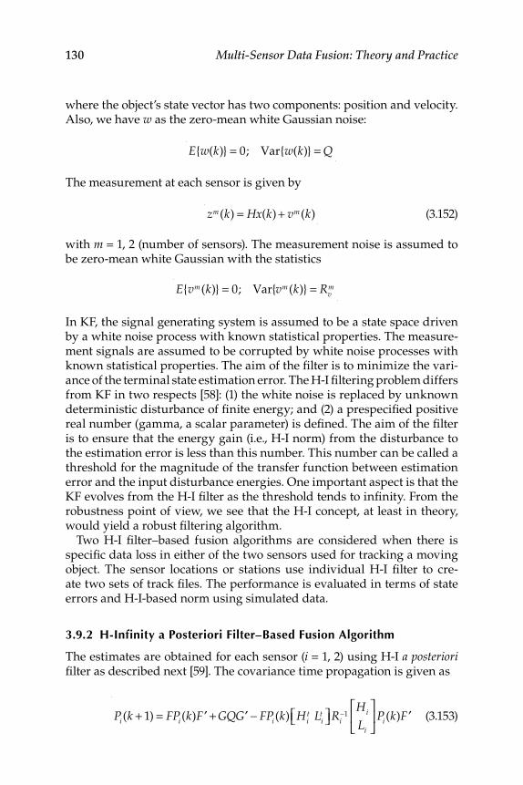
130 Multi-Sensor Data Fusion: Theory and Practice

where the object’s state vector has two components: position and velocity. Also, we have w as the zero-mean white Gaussian noise:

E{w(k)} = 0; Var{w(k)} = Q

The measurement at each sensor is given by

z

m(k) = Hx(k) + vm(k) (3.152)

with m = 1, 2 (number of sensors). The measurement noise is assumed to be zero-mean white Gaussian with the statistics

E{vm(k)} = 0; Var{vm(k)} = Rv

m

In KF, the signal generating system is assumed to be a state space driven by a white noise process with known statistical properties. The measure-ment signals are assumed to be corrupted by white noise processes with known statistical properties. The aim of the fi lter is to minimize the vari-ance of the terminal state estimation error. The H-I fi ltering problem differs from KF in two respects [58]: (1) the white noise is replaced by unknown deterministic disturbance of fi nite energy; and (2) a prespecifi ed positive real number (gamma, a scalar parameter) is defi ned. The aim of the fi lter is to ensure that the energy gain (i.e., H-I norm) from the disturbance to the estimation error is less than this number. This number can be called a threshold for the magnitude of the transfer function between estimation error and the input disturbance energies. One important aspect is that the KF evolves from the H-I fi lter as the threshold tends to infi nity. From the robustness point of view, we see that the H-I concept, at least in theory, would yield a robust fi ltering algorithm.

Two H-I fi lter–based fusion algorithms are considered when there is specifi c data loss in either of the two sensors used for tracking a moving object. The sensor locations or stations use individual H-I fi lter to cre-ate two sets of track fi les. The performance is evaluated in terms of state errors and H-I-based norm using simulated data.

3.9.2 H-Infinity a Posteriori Filter–Based Fusion Algorithm

The estimates are obtained for each sensor ( i = 1, 2) using H-I a posteriori fi lter as described next [59]. The covariance time propagation is given as

Pi (k + 1) = FPi (k) ′F + GQ ′G − FPi (k) Hi

t Lit⎡⎣ ⎤⎦ Ri

−1Hi

Li

⎡

⎣⎢

⎤

⎦⎥ Pi (k) ′F (3.153)

Strategies and Algorithms for Target Tracking and Data Fusion 131

Ri =

I 0

0 −γ 2I

⎡

⎣⎢

⎤

⎦⎥ +

Hi

Li

⎡

⎣⎢

⎤

⎦⎥ Pi (k) Hi

t Lit⎡⎣ ⎤⎦ (3.154)

The H-I fi lter gain is given as

Ki = Pi (k + 1)Hi

t I + HiPi (k + 1)Hit( )−1

(3.155)

The measurement update of states is obtained by

xi (k + 1) = Fxi (k) + Ki yi (k + 1) − HiFxi (k)( ) (3.156)

The conditions for the existence of the H-I fi lters are given in [59]. The fusion of the estimates from the two sensors then can be obtained by

x f (k + 1) = x

1(k + 1) + P

1(k + 1) P

1(k + 1) + P

2(k + 1)( )−1

× x

2(k + 1) − x

1(k + 1)( )

(3.157)

Pf (k + 1) = P

1(k + 1) − P

1(k + 1) P

1(k + 1) + P

2(k + 1)( )−1

P1t (k + 1) (3.158)

The fused state vector and the covariance of the fused state utilize the indi-vidual estimate state vectors (of each sensor) and covariance matrices.

3.9.3 H-Infinity Global Fusion Algorithm

This fi ltering algorithm is based on [60,61]. The local fi lters are given for each sensor ( i = 1, 2,..., m ).

State and ovariance time propagation is given by

%xi (k + 1) = Fxi (k) (3.159)

%Pi (k + 1) = FPi (k)F '+ GQG ' (3.160)

The covariance update is given by

Pi

−1(k + 1) = %Pi−1(k + 1) + Hi

t Lit⎡⎣ ⎤⎦

I 0

0 −γ 2I

⎡

⎣⎢

⎤

⎦⎥

−1Hi

Li

⎡

⎣⎢

⎤

⎦⎥ (3.161)

The local fi lter gains are given as

Ai = I + 1/γ 2 Pi (k + 1)Li

t Li ; Ki = Ai−1Pi (k + 1)Hi

t (3.162)

132 Multi-Sensor Data Fusion: Theory and Practice

The measurement update of local states is given as

xi (k + 1) = %xi (k + 1) + Ki yi (k + 1) − Hi

%xi (k + 1)( ) (3.163)

The time propagation of fusion state and covariance is given as

%x f (k + 1) = Fx f (k) (3.164)

%Pf (k + 1) = FPf (k)F '+ GQG ' (3.165)

The measurement update of the fusion states and covariance is

Pf

−1(k + 1) = %Pf−1(k + 1) + Pi

−1(k + 1) − %Pi−1(k + 1)( ) + m − 1

γ 2i=1

m

∑ LtL (3.166)

The global gain is

Af = I + 1/γ 2 Pf (k + 1)LtL (3.167)

The global (measurement update) fused state is

x f (k + 1) = I − Af−1Pf (k + 1)H f

t H f⎡⎣ ⎤⎦ %x f (k + 1) + Af

−1Pf (k + 1)

Pi−1(k + 1)Aixi (k + 1) − Pi

−1(k + 1)Ai + HitHi( )Fxi (k){ }

i=1

m

∑

(3.168)

3.9.4 Numerical Simulation Results

The simulated data are generated in PC MATLAB for a tracking prob-lem [62]. The normalized random noise is added to the state vector and the measurements of each sensor are corrupted with random noise. The sensors could have dissimilar measurement noise variances (e.g., sen-sor 2 having higher variance than sensor 1). The initial condition for the state vector is x (0) = [200 0.5]. The performance of the fusion fi lters is also evaluated in terms of H-I norm. This ratio (the H-I norm) should be less than square of gamma, which can be considered an upper bound on the maximum energy gain from the input to the output. The output

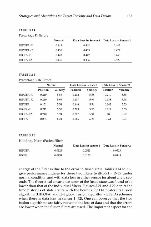
Strategies and Algorithms for Target Tracking and Data Fusion 133

energy of the fi lter is due to the error in fused state. Tables 3.14 to 3.16 give performance indices for these two fi lters (with Rv1 = Rv2): under normal condition and with data loss in either sensor for about a few sec-onds. The theoretical covariance norm of the fused state was found to be lower than that of the individual fi lters. Figures 3.21 and 3.22 depict the time histories of state errors with the bounds for H-I posteriori fusion algorithm (HIPOFA) and H-I global fusion algorithm (HIGFA) schemes when there is data loss in sensor 1 [62]. One can observe that the two fusion algorithms are fairly robust to the loss of data and that the errors are lower when the fusion fi lters are used. The important aspect for the

TABLE 3.14

Percentage Fit Errors

Normal Data Loss in Sensor 1 Data Loss in Sensor 2

HIPOFA-F1 0.443 0.442 0.443

HIPOFA-F2 0.435 0.435 0.427

HIGFA-F1 0.443 0.442 0.443

HIGFA-F2 0.436 0.436 0.427

TABLE 3.16

H-Infi nity Norm (Fusion Filter)

Normal Data Loss in sensor 1 Data Loss in Sensor 2

HIPOFA 0.0523 0.0523 0.0523

HIGFA 0.0151 0.0155 0.0145

TABLE 3.15

Percentage State Errors

Normal Data Loss in Sensor 1 Data Loss in Sensor 2

Position Velocity Position Velocity Position Velocity

HIPOFA-F1 0.210 5.56 0.202 5.55 0.210 5.55

HIPOFA-F2 0.210 5.99 0.207 5.99 0.188 5.98

HIPOFA 0.151 5.54 0.146 5.54 0.142 5.53

HIGFA-L1 0.211 5.55 0.203 5.55 0.211 5.55

HIGFA-L2 0.210 5.94 0.207 5.94 0.188 5.92

HIGFA 0.065 6.24 0.066 6.24 0.064 6.24

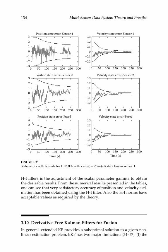
134 Multi-Sensor Data Fusion: Theory and Practice

H-I fi lters is the adjustment of the scalar parameter gamma to obtain the desirable results. From the numerical results presented in the tables, one can see that very satisfactory accuracy of position and velocity esti-mation has been obtained using the H-I fi lter. Also the H-I norms have acceptable values as required by the theory.

3.10 Derivative-Free Kalman Filters for Fusion

In general, extended KF provides a suboptimal solution to a given non-linear estimation problem. EKF has two major limitations [34–37]: (1) the

FIGURE 3.21 State errors with bounds for HIPOFA with var( v 2) = 9*var( v 1); data loss in sensor 1.

0 50 100 150 200 250 300-3-2-1

0123

0 50 100 150 200 250 300

0 50 100 150 200 250 300 0 50 100 150 200 250 300

0 50 100 150 200 250 300 0 50 100 150 200 250 300

-3-2-1

0123

-0.2-0.1

00.10.20.3

-0.2-0.1

00.10.20.3

-0.2-0.1

00.10.20.3

-3-2-1

0123

Position state error-Sensor 1 Velocity state error-Sensor 1

Position state error-Sensor 2 Velocity state error-Sensor 2

Velocity state error-FusedPosition state error-Fused

Time (s)Time (s)

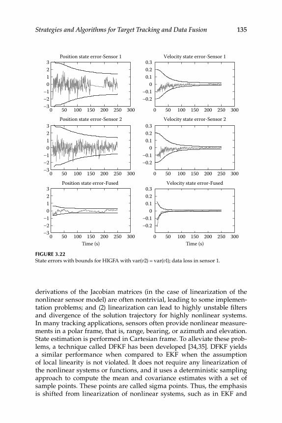
Strategies and Algorithms for Target Tracking and Data Fusion 135

derivations of the Jacobian matrices (in the case of linearization of the nonlinear sensor model) are often nontrivial, leading to some implemen-tation problems; and (2) linearization can lead to highly unstable fi lters and divergence of the solution trajectory for highly nonlinear systems. In many tracking applications, sensors often provide nonlinear measure-ments in a polar frame, that is, range, bearing, or azimuth and elevation. State estimation is performed in Cartesian frame. To alleviate these prob-lems, a technique called DFKF has been developed [34,35]. DFKF yields a similar performance when compared to EKF when the assumption of local linearity is not violated. It does not require any linearization of the nonlinear systems or functions, and it uses a deterministic sampling approach to compute the mean and covariance estimates with a set of sample points. These points are called sigma points. Thus, the emphasis is shifted from linearization of nonlinear systems, such as in EKF and

FIGURE 3.22 State errors with bounds for HIGFA with var( v 2) = var( v 1); data loss in sensor 1.

0 50 100 150 200 250 300 0 50 100 150 200 250 300-3-2-1

0123

-0.2-0.1

00.10.20.3

0 50 100 150 200 250 300-3-2-1

0123

0 50 100 150 200 250 300-3-2-1

0123

Position state error-Sensor 1 Velocity state error-Sensor 1

0 50 100 150 200 250 300

-0.2-0.1

00.10.20.3

Velocity state error-Sensor 2

0 50 100 150 200 250 300

-0.2-0.1

00.10.20.3

Position state error-Sensor 2

Velocity state error-Fused

Time (s)Time (s)

Position state error-Fused

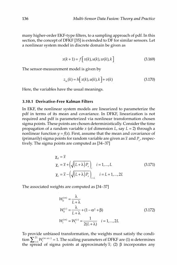
136 Multi-Sensor Data Fusion: Theory and Practice

many higher-order EKF-type fi lters, to a sampling approach of pdf. In this section, the concept of DFKF [35] is extended to DF for similar sensors. Let a nonlinear system model in discrete domain be given as

x(k + 1) = f x(k), u(k), w(k), k⎡⎣ ⎤⎦ (3.169)

The sensor-measurement model is given by

zm(k) = h x(k), u(k), k⎡⎣ ⎤⎦ + v(k) (3.170)

Here, the variables have the usual meanings.

3.10.1 Derivative-Free Kalman Filters

In EKF, the nonlinear system models are linearized to parameterize the pdf in terms of its mean and covariance. In DFKF, linearization is not required and pdf is parameterized via nonlinear transformation chosen sigma points. These points are chosen deterministically. Consider the time propagation of a random variable x (of dimension L , say L = 2) through a nonlinear function y = f(x) . First, assume that the mean and covariance of (primarily) sigma points for random variable are given as x and Px , respec-tively. The sigma points are computed as [34–37]

χ0

= x

χi = x + L + λ( )Px( )i

i = 1,..., L

χi = x − L + λ( )Px( )i−L

i = L + 1,..., 2L

(3.171)

The associated weights are computed as [34–37]

W0

(m) = λL + λ

W0

(c) = λL + λ

+ (1 − α2 + β)

Wi(m) = Wi

(c) = 1

2(L + λ)i = 1,..., 2L

(3.172)

To provide unbiased transformation, the weights must satisfy the condi-

tion Wi(m or c)

i=1

2L∑ = 1. The scaling parameters of DFKF are (1) α determines the spread of sigma points at approximately x; (2) β incorporates any

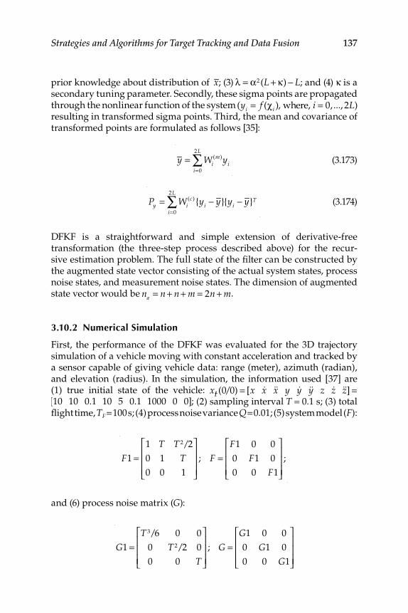
Strategies and Algorithms for Target Tracking and Data Fusion 137

prior knowledge about distribution of x; (3) λ = α2 (L + κ) − L; and (4) κ is a secondary tuning parameter. Secondly, these sigma points are propagated through the nonlinear function of the system (yi = f (χi ), where, i = 0,..., 2L)resulting in transformed sigma points. Third, the mean and covariance of transformed points are formulated as follows [35]:

y = Wi

(m)yii=0

2L

∑ (3.173)

Py = Wi

(c) {yi − y}{yi − y}T

i=0

2L

∑ (3.174)

DFKF is a straightforward and simple extension of derivative-free transformation (the three-step process described above) for the recur-sive estimation problem. The full state of the fi lter can be constructed by the augmented state vector consisting of the actual system states, process noise states, and measurement noise states. The dimension of augmented state vector would be na = n + n + m = 2n + m.

3.10.2 Numerical Simulation

First, the performance of the DFKF was evaluated for the 3D trajectory simulation of a vehicle moving with constant acceleration and tracked by a sensor capable of giving vehicle data: range (meter), azimuth (radian), and elevation (radius). In the simulation, the information used [37] are (1) true initial state of the vehicle: xt(0/0) = [x &x &&x y &y &&y z &z &&z] = [10 10 0.1 10 5 0.1 1000 0 0]; (2) sampling interval T = 0.1 s; (3) total fl ight time, T F = 100 s; (4) process noise variance Q = 0.01; (5) system model (F) :

F1 =1 T T 2/2

0 1 T

0 0 1

⎡

⎣

⎢⎢⎢

⎤

⎦

⎥⎥⎥

; F =F1 0 0

0 F1 0

0 0 F1

⎡

⎣

⎢⎢⎢

⎤

⎦

⎥⎥⎥

;

and (6) process noise matrix ( G) :

G1 =T 3/6 0 0

0 T 2/2 0

0 0 T

⎡

⎣

⎢⎢⎢

⎤

⎦

⎥⎥⎥

; G =G1 0 0

0 G1 0

0 0 G1

⎡

⎣

⎢⎢⎢

⎤

⎦

⎥⎥⎥

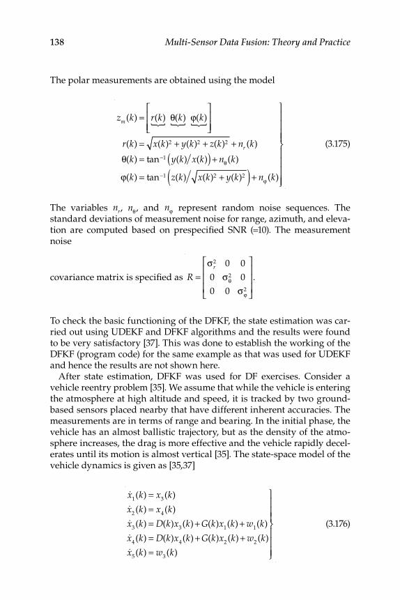
138 Multi-Sensor Data Fusion: Theory and Practice

The polar measurements are obtained using the model

zm(k) = r(k){ θ(k){ ϕ(k){⎡

⎣⎢⎢

⎤

⎦⎥⎥

r(k) = x(k)2 + y(k)2 + z(k)2 + nr (k)

θ(k) = tan−1 y(k) x(k)( ) + nθ(k)

ϕ(k) = tan−1 z(k) x(k)2 + y(k)2( ) + nϕ (k)

⎫

⎬

⎪⎪⎪⎪

⎭

⎪⎪⎪⎪

(3.175)

The variables nr, nθ, and nϕ represent random noise sequences. The standard deviations of measurement noise for range, azimuth, and eleva-tion are computed based on prespecifi ed SNR (=10). The measurement noise

covariance matrix is specifi ed as

R =σr

2 0 0

0 σθ2 0

0 0 σϕ2

⎡

⎣

⎢⎢⎢

⎤

⎦

⎥⎥⎥.

To check the basic functioning of the DFKF, the state estimation was car-ried out using UDEKF and DFKF algorithms and the results were found to be very satisfactory [37]. This was done to establish the working of the DFKF (program code) for the same example as that was used for UDEKF and hence the results are not shown here.

After state estimation, DFKF was used for DF exercises. Consider a vehicle reentry problem [35]. We assume that while the vehicle is entering the atmosphere at high altitude and speed, it is tracked by two ground-based sensors placed nearby that have different inherent accuracies. The measurements are in terms of range and bearing. In the initial phase, the vehicle has an almost ballistic trajectory, but as the density of the atmo-sphere increases, the drag is more effective and the vehicle rapidly decel-erates until its motion is almost vertical [35]. The state-space model of the vehicle dynamics is given as [35,37]

&x1(k) = x

3(k)

&x2(k) = x

4(k)

&x3(k) = D(k)x

3(k) + G(k)x

1(k) + w

1(k)

&x4(k) = D(k)x

4(k) + G(k)x

2(k) + w

2(k)

&x5(k) = w

3(k)

⎫

⎬

⎪⎪⎪

⎭

⎪⎪⎪

(3.176)

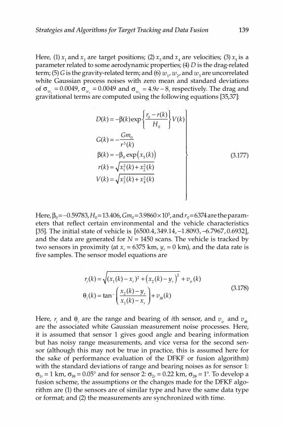
Strategies and Algorithms for Target Tracking and Data Fusion 139

Here, (1) x1and x

2are target positions; (2) x

3and x

4 are velocities; (3) x5is a

parameter related to some aerodynamic properties; (4) D is the drag-related term; (5) G is the gravity-related term; and (6) w

1, w

2, and w

3 are uncorrelated

white Gaussian process noises with zero mean and standard deviations of σw1

= 0.0049, σw1= 0.0049 and σw1

= 4.9e − 8, respectively. The drag and gravitational terms are computed using the following equations [35,37]:

D(k) = −β(k)expr0

− r(k)

H0

⎧⎨⎩

⎫⎬⎭

V(k)

G(k) = −Gm

0

r3 (k)

β(k) = −β0

exp x5(k)( )

r(k) = x12 (k) + x

22 (k)

V(k) = x32 (k) + x

42 (k)

⎫

⎬

⎪⎪⎪⎪⎪⎪

⎭

⎪⎪⎪⎪⎪⎪

(3.177)

Here, β 0 = −0.59783, H 0 = 13.406, Gm 0 = 3.9860 × 10 5 , and r 0 = 6374 are the param-eters that refl ect certain environmental and the vehicle characteristics [35]. The initial state of vehicle is [6500.4, 349.14, −1.8093, −6.7967, 0.6932], and the data are generated for N = 1450 scans. The vehicle is tracked by two sensors in proximity (at x r = 6375 km, y r = 0 km), and the data rate is fi ve samples. The sensor model equations are

ri (k) = (x1(k) − xr )2 + x

2(k) − yr( )2

+ vir (k)

θi (k) = tan− x2(k) − yr

x1(k) − xr

⎛⎝⎜

⎞⎠⎟

+ viθ(k)

(3.178)

Here, ri and θi are the range and bearing of i th sensor, and vir and viθare the associated white Gaussian measurement noise processes. Here, it is assumed that sensor 1 gives good angle and bearing information but has noisy range measurements, and vice versa for the second sen-sor (although this may not be true in practice, this is assumed here for the sake of performance evaluation of the DFKF or fusion algorithm) with the standard deviations of range and bearing noises as for sensor 1: σ 1 r = 1 km, σ 1 θ = 0.05° and for sensor 2: σ 2 r = 0.22 km, σ 2 θ = 1°. To develop a fusion scheme, the assumptions or the changes made for the DFKF algo-rithm are (1) the sensors are of similar type and have the same data type or format; and (2) the measurements are synchronized with time.

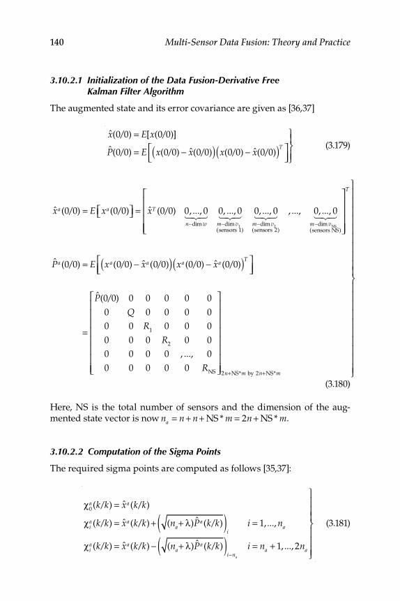
140 Multi-Sensor Data Fusion: Theory and Practice

3.10.2.1 Initialization of the Data Fusion-Derivative Free Kalman Filter Algorithm

The augmented state and its error covariance are given as [36,37]

x(0/0) = E[x(0/0)]

P(0/0) = E x(0/0) − x(0/0)( ) x(0/0) − x(0/0)( )T⎡⎣⎢

⎤⎦⎥

⎫⎬⎪

⎭⎪

(3.179)

xa (0/0) = E xa (0/0)⎡⎣ ⎤⎦ = xT (0/0) 0, ..., 0n−dim w123 0, ..., 0

m−dim v1(sensors 1)

123 0, ..., 0m−dim v2(sensors 2)

123 , ..., 0, ..., 0m−dim vNS(sensors NS)

123

⎡

⎣

⎢⎢⎢⎢

⎤

⎦

⎥⎥⎥⎥

T

Pa (0/0) = E xa(0/0) − xa (0/0)( ) xa (0/0) − xa (0/0)( )T⎡⎣⎢

⎤⎦⎥

=

P(0/0) 0 0 0 0 0

0 Q 0 0 0 00 0 R1 0 0 0

0 0 0 R2 0 00 0 0 0 , ..., 0

0 0 0 0 0 RNS

⎡

⎣

⎢⎢⎢⎢⎢⎢⎢⎢

⎤

⎦

⎥⎥⎥⎥⎥⎥⎥⎥2n+NS*m by 2n+NS*m

⎫

⎬

⎪⎪⎪⎪⎪⎪⎪⎪⎪⎪

⎭

⎪⎪⎪⎪⎪⎪⎪⎪⎪⎪

(3.180)

Here, NS is the total number of sensors and the dimension of the aug-mented state vector is now na = n + n + NS * m = 2n + NS * m.

3.10.2.2 Computation of the Sigma Points

The required sigma points are computed as follows [35,37]:

χ0a (k/k) = xa (k/k)

χia (k/k) = xa (k/k) + (na+ λ)Pa (k/k)( )

ii = 1,..., na

χia (k/k) = xa (k/k) − (na+ λ)Pa (k/k)( )

i−na

i = na + 1,..., 2na

⎫

⎬

⎪⎪⎪

⎭

⎪⎪⎪

(3.181)

Strategies and Algorithms for Target Tracking and Data Fusion 141

Here,

χa = χstate

{ χw{ χv1

{χv2

{ , ..., χvNS

{⎡

⎣⎢⎢

⎤

⎦⎥⎥. The augmented states are those of

the measurement data noise processes.

3.10.2.3 State and Covariance Propagation

The state and covariance equations are given as [35,37]

χ(k + 1/k) = f χ(k/k), u(k), χw (k/k), k( )%x(k + 1/k) = Wi

(m)

i=0

2na

∑ χi (k + 1/k)

%P(k + 1/k) = Wi(c) χi (k + 1/k) − %x(k + 1/k)⎡⎣ ⎤⎦

i=0

2na

∑ χi (k + 1/k) − %x(k + 1/k)⎡⎣ ⎤⎦T

⎫

⎬

⎪⎪⎪⎪

⎭

⎪⎪⎪⎪

(3.182)

W0

(m) = λna + λ

W0

(c) = λna + λ

+ (1 − α2 + β)

Wi(m) = Wi

(c) = 1

2(na + λ)i = 1,..., 2na

⎫

⎬

⎪⎪⎪

⎭

⎪⎪⎪

(3.183)

3.10.2.4 State and Covariance Update

The measurement update equations for the state and covariance are given as [35,37]

y j (k + 1/k) = h χ(k/k), u(k), k( ) + χvj (k/k)

%z j (k + 1/k) = Wi(m)yi

j (k + 1/k)i=0

2na

∑

⎫

⎬⎪

⎭⎪

(3.184)

Here, j = 1,..., NS and

y(k + 1/k) = y1(k + 1/k) y2 (k + 1/k) , ..., yNS (k + 1/k)⎡⎣ ⎤⎦T

%z(k + 1/k) = %z1(k + 1/k) %z2 (k + 1/k) , ..., %zNS (k + 1/k)⎡⎣ ⎤⎦T

(3.185)

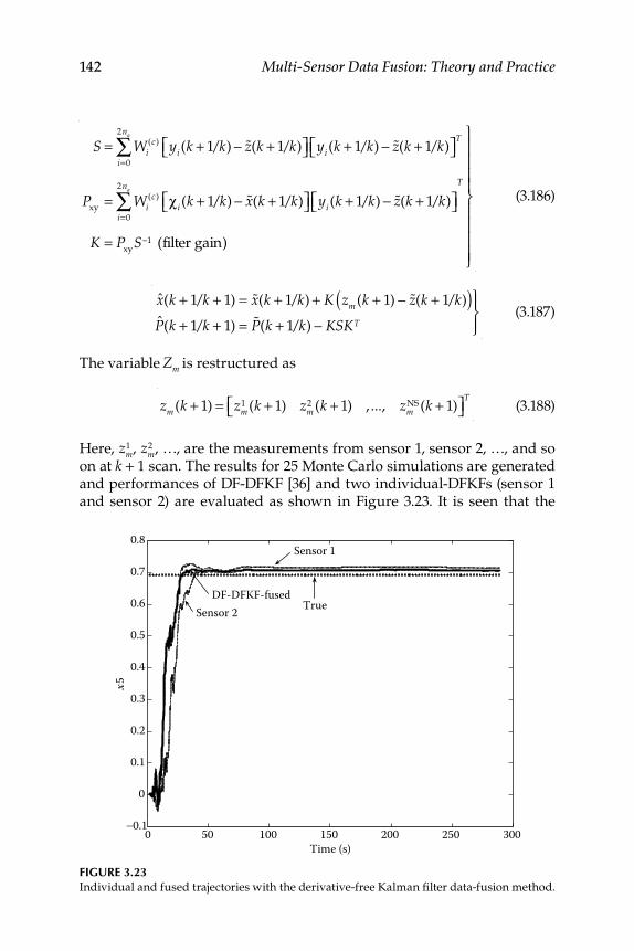
142 Multi-Sensor Data Fusion: Theory and Practice

S = Wi(c) yi (k + 1/k) − %z(k + 1/k)⎡⎣ ⎤⎦ yi (k + 1/k) − %z(k + 1/k)⎡⎣ ⎤⎦

T

i=0

2na

∑

Pxy

= Wi(c) χi (k + 1/k) − %x(k + 1/k)⎡⎣ ⎤⎦ yi (k + 1/k) − %z(k + 1/k)⎡⎣ ⎤⎦

i=0

2na

∑T

K = Pxy

S−1 (filter gain)

⎫

⎬

⎪⎪⎪⎪

⎭

⎪⎪⎪⎪

(3.186)

x(k + 1/k + 1) = %x(k + 1/k) + K zm(k + 1) − %z(k + 1/k)( )P(k + 1/k + 1) = %P(k + 1/k) − KSKT

⎫⎬⎪

⎭⎪ (3.187)

The variable Zm is restructured as

zm(k + 1) = zm

1 (k + 1) zm2 (k + 1) , ..., zm

NS (k + 1)⎡⎣ ⎤⎦T

(3.188)

Here, zm1 , zm

2 , …, are the measurements from sensor 1, sensor 2, …, and so on at k + 1 scan. The results for 25 Monte Carlo simulations are generated and performances of DF-DFKF [36] and two individual-DFKFs (sensor 1 and sensor 2) are evaluated as shown in Figure 3.23. It is seen that the

FIGURE 3.23 Individual and fused trajectories with the derivative-free Kalman fi lter data-fusion method.

0 50 100 150 200 250 300-0.1

0

0.1

0.2

0.3

0.4

0.5

0.6

0.7

0.8

x5

TrueDF-DFKF-fused

Sensor 2

Sensor 1

Time (s)

Strategies and Algorithms for Target Tracking and Data Fusion 143

fused state as compared to the estimated state from other two fi lters is closer to the true state [37].

3.11 Missile Seeker Estimator

In interceptors active radar seeker is used to measure: (1) relative range, (2) relative range rate, (3) line-of-sight (LOS) angles, and (4) rates between interceptor and evader. The measurements are contaminated by a high degree of noise due to glint, radar cross section (RCS) fl uctuation, and thermal noise. The true LOS rates have to be estimated for proportional navigation (PN) guidance of the interceptor [63,64]. Advanced proportional navigation (APN) guidance control systems would also use target acceler-ation. An estimator or seeker fi lter is required, which processes the seeker measurements recursively to obtain the signals required for guidance of the interceptor towards the evader or target. The design of the estimator is complex because the cumulative effects of the noise are non- Gaussian and time correlated. There would also be a periodic loss of seeker measure-ments due to target eclipsing effects. Since the seeker measurements are available in the inner Gimbal frame, one would need an EKF for the seeker estimator. To handle non-Gaussian noise, an augmented EKF (AEKF) is used. In interceptor-evading target engagement scenarios or games, the evader would execute maneuvers—perhaps unpredictably—to avoid the interceptor. To track such a maneuvering target, an IMM model is gener-ally used. The IMM is an adaptive estimator that is based on the assump-tion of the use of a fi nite number of models [65]. In this section, an IMM based on the soft switching between a set of predefi ned (evader target) models such as constant velocity, constant acceleration, and constant jerk [66] is described. At each sampling time, the mode probability is computed for each model using innovation-vector and covariance matrix. Each of the mode matched fi lter is based on the AEKF. The new fi lter is expected to give better performance in an engagement scenario [67,68]. The per-formance evaluation of an IMM-AEKF in a closed-loop, using MATLAB simulated data of a typical interceptor–evader engagement scenario, is discussed.

3.11.1 Interacting Multiple Model–Augmented Extended Kalman Filter Algorithm

The state vector of respective mode-matched fi lter is augmented with additional states for handling glint noise and RCS fl uctuations.

144 Multi-Sensor Data Fusion: Theory and Practice

3.11.1.1 State Model

The state vector consists of 18 states (with six states related to glint noise and RCS fl uctuations):

Δx ΔVx atx jtx Δy ΔVy aty jty

⎡⎣

Δz ΔVz atz jtz RCS and Glint states⎤⎦

The mathematical models for glint and RCS are given next [63,67,68]. State model 1, constant velocity (CV) model:

Δ &x = ΔVx ; Δ &Vx = 0; &atx = 0; &jtx = 0

Δ &y = ΔVy ; Δ &Vy = 0; &aty = 0; &jty = 0

Δ&z = ΔVz ; Δ &Vz = 0; &atz = 0; &jjz = 0

(3.189)

State model 2, constant acceleration (CA) model:

Δ &x = ΔVx ; Δ &Vx = atx − amx ; &atx = −atx

τx

⎛⎝⎜

⎞⎠⎟

; &jtx = 0; Δ &y = ΔVy ;

Δ &Vy = aty − amy ; &aty = −aty

τy

⎛

⎝⎜

⎞

⎠⎟ ; &jty = 0;

Δ&z = ΔVz ; Δ &Vz = atz − amz ; &atz = −atz

τz

⎛⎝⎜

⎞⎠⎟

; &jjz = 0

(3.190)

State model 3, constant jerk (CJ) model:

Δ &x = ΔVx ; Δ &Vx = atx − amx ; &atx = jtx ; &jtx = −jtx

τx

⎛⎝⎜

⎞⎠⎟

Δ &y = ΔVy ; Δ &Vy = aty − amy ; &aty = jty ; &jty = −jty

τy

⎛

⎝⎜

⎞

⎠⎟

Δ&z = ΔVz ; Δ &Vz = atz − amz ; &atz = jtz ; &jjz = −jtz

τz

⎛⎝⎜

⎞⎠⎟

(3.191)

In Equations 3.189 to 3.191, Δ x , Δ y , and Δ z are the relative positions and Δ V x , Δ V y , and Δ V z are the relative velocities of target with respect to mis-sile, a tx , a ty , and a tz are the target accelerations, J tx , J ty , and J tz are the target jerks, a mx , a my , and a mz are the missile accelerations, and τ x , τ y , and τ z are the correlation time constants.

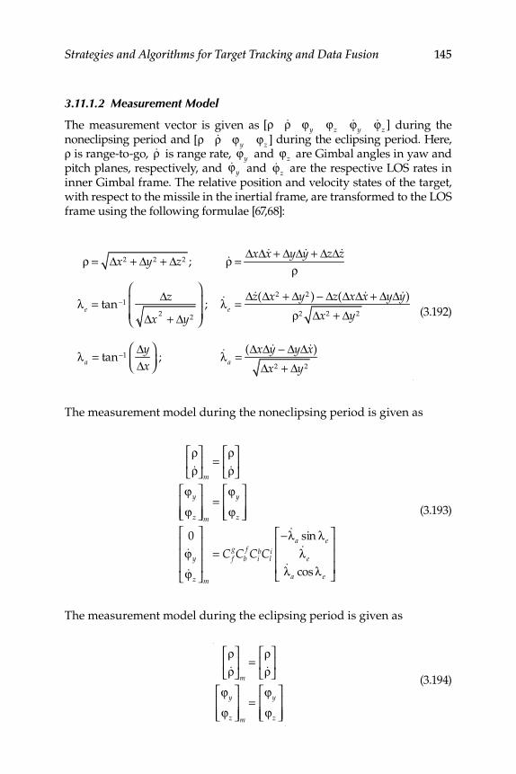
Strategies and Algorithms for Target Tracking and Data Fusion 145

3.11.1.2 Measurement Model

The measurement vector is given as [ρ &ρ ϕy ϕz&ϕy

&ϕz ] during the non eclipsing period and [ρ &ρ ϕy ϕz ] during the eclipsing period. Here, ρ is range-to-go, &ρ is range rate, ϕy and ϕz are Gimbal angles in yaw and pitch planes, respectively, and &ϕy and &ϕz are the respective LOS rates in inner Gimbal frame. The relative position and velocity states of the target, with respect to the missile in the inertial frame, are transformed to the LOS frame using the following formulae [67,68]:

ρ = Δx2 + Δy2 + Δz2 ; &ρ =ΔxΔ&x + ΔyΔ &y + ΔzΔ&z

ρ

λe = tan−1Δz

Δx2 + Δy2

⎛

⎝⎜⎜

⎞

⎠⎟⎟

; &λe =Δ&z(Δx2 + Δy2 ) − Δz(ΔxΔ&x + ΔyΔ &y)

ρ2 Δx2 + Δy2

λa = tan−1ΔyΔx

⎛⎝⎜

⎞⎠⎟

; &λa =(ΔxΔ &y − ΔyΔ&x)

Δx2 + Δy2

(3.192)

The measurement model during the noneclipsing period is given as

ρ&ρ⎡

⎣⎢⎤

⎦⎥

m

=ρ&ρ⎡

⎣⎢⎤

⎦⎥

ϕy

ϕz

⎡

⎣⎢⎢

⎤

⎦⎥⎥m

=ϕy

ϕz

⎡

⎣⎢⎢

⎤

⎦⎥⎥

0&ϕy

&ϕz

⎡

⎣

⎢⎢⎢

⎤

⎦

⎥⎥⎥

m

= C fgCb

f CibCl

i

− &λa sinλe&λ e

&λa cosλ e

⎡

⎣

⎢⎢⎢

⎤

⎦

⎥⎥⎥

(3.193)

The measurement model during the eclipsing period is given as

ρ&ρ

⎡

⎣⎢

⎤

⎦⎥

m

=ρ&ρ

⎡

⎣⎢

⎤

⎦⎥

ϕy

ϕz

⎡

⎣⎢⎢

⎤

⎦⎥⎥m

=ϕy

ϕz

⎡

⎣⎢⎢

⎤

⎦⎥⎥

(3.194)

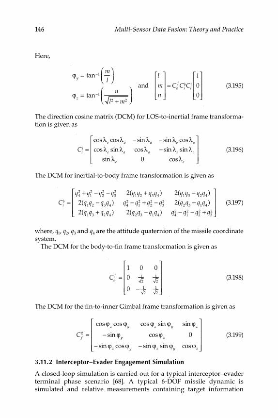
146 Multi-Sensor Data Fusion: Theory and Practice

Here,

ϕy = tan−1ml

⎛⎝⎜

⎞⎠⎟

ϕz = tan−1n

l2 + m2

⎛⎝⎜

⎞⎠⎟

and

l

m

n

⎡

⎣

⎢⎢⎢

⎤

⎦

⎥⎥⎥

= Cbf Ci

bCli

1

0

0

⎡

⎣

⎢⎢⎢

⎤

⎦

⎥⎥⎥

(3.195)

The direction cosine matrix (DCM) for LOS-to-inertial frame transforma-tion is given as

Cli =

cos λe cos λa − sin λa − sin λe cos λa

cos λe sin λa cos λa − sin λe sin λa

sin λe 0 cos λe

⎡

⎣

⎢⎢⎢

⎤

⎦

⎥⎥⎥

(3.196)

The DCM for inertial-to-body frame transformation is given as

Cib =

q42 + q

12 − q

22 − q

32 2(q

1q

2+ q

3q

4) 2(q

1q

3− q

2q

4)

2(q1q

2− q

3q

4) q

42 − q

12 + q

22 − q

32 2(q

2q

3+ q

1q

4)

2(q1q

3+ q

2q

4) 2(q

2q

3− q

1q

4) q

42 − q

12 − q

22 + q

32

⎡

⎣

⎢⎢⎢

⎤

⎦

⎥⎥⎥

(3.197)

where, q 1 , q 2 , q 3 and q 4 are the attitude quaternion of the missile coordinate system.

The DCM for the body-to-fi n frame transformation is given as

Cbf =

1 0 0

0 1

2

1

2

0 − 1

2

1

2

⎡

⎣

⎢⎢⎢⎢

⎤

⎦

⎥⎥⎥⎥

(3.198)

The DCM for the fi n-to-inner Gimbal frame transformation is given as

C fg =

cosϕz cosϕy cosϕz sinϕy sinϕz

− sinϕy cosϕz 0

− sinϕz cosϕy − sinϕz sinϕy cosϕz

⎡

⎣

⎢⎢⎢⎢

⎤

⎦

⎥⎥⎥⎥

(3.199)

3.11.2 Interceptor–Evader Engagement Simulation

A closed-loop simulation is carried out for a typical interceptor–evader terminal phase scenario [68]. A typical 6-DOF missile dynamic is simulated and relative measurements containing target information

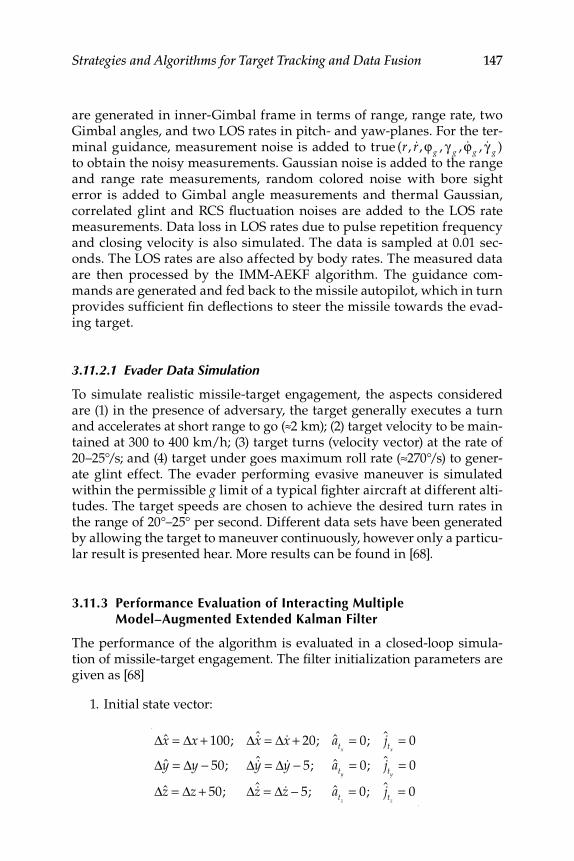
Strategies and Algorithms for Target Tracking and Data Fusion 147

are generated in inner-Gimbal frame in terms of range, range rate, two Gimbal angles, and two LOS rates in pitch- and yaw-planes. For the ter-minal guidance, measurement noise is added to true (r, &r,ϕg , γ g , &ϕg , &γ g )to obtain the noisy measurements. Gaussian noise is added to the range and range rate measurements, random colored noise with bore sight error is added to Gimbal angle measurements and thermal Gaussian, correlated glint and RCS fl uctuation noises are added to the LOS rate measurements. Data loss in LOS rates due to pulse repetition frequency and closing velocity is also simulated. The data is sampled at 0.01 sec-onds. The LOS rates are also affected by body rates. The measured data are then processed by the IMM-AEKF algorithm. The guidance com-mands are generated and fed back to the missile autopilot, which in turn provides suffi cient fi n defl ections to steer the missile towards the evad-ing target.

3.11.2.1 Evader Data Simulation

To simulate realistic missile-target engagement, the aspects considered are (1) in the presence of adversary, the target generally executes a turn and accelerates at short range to go (≈2 km); (2) target velocity to be main-tained at 300 to 400 km/h; (3) target turns (velocity vector) at the rate of 20–25°/s; and (4) target under goes maximum roll rate (≈270°/s) to gener-ate glint effect. The evader performing evasive maneuver is simulated within the permissible g limit of a typical fi ghter aircraft at different alti-tudes. The target speeds are chosen to achieve the desired turn rates in the range of 20°–25° per second. Different data sets have been generated by allowing the target to maneuver continuously, however only a particu-lar result is presented hear. More results can be found in [68].

3.11.3 Performance Evaluation of Interacting Multiple Model–Augmented Extended Kalman Filter

The performance of the algorithm is evaluated in a closed-loop simula-tion of missile-target engagement. The fi lter initialization parameters are given as [68]

1. Initial state vector:

Δx = Δx + 100; Δ &x = Δ &x + 20; atx= 0; jtx

= 0

Δy = Δy − 50; Δ &y = Δ &y − 5; aty= 0; jty

= 0

Δz = Δz + 50; Δ &z = Δ&z − 5; atz= 0; jtz

= 0

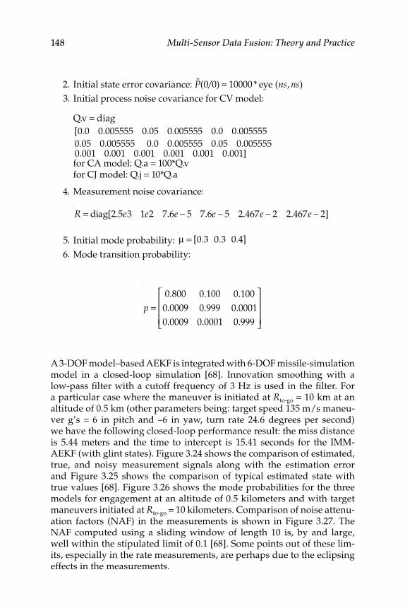
148 Multi-Sensor Data Fusion: Theory and Practice

2. Initial state error covariance: P(0/0) = 10000 * eye (ns, ns)

3. Initial process noise covariance for CV model:

Q.v = diag

[0.0 0.005555 0.05 0.005555 0.0 0.005555

0.05 0.005555 0.0 0.005555 0.05 0.0055550.001 0.001 0.001 0.001 0.001 0.001] for CA model: Q.a = 100*Q.v for CJ model: Q.j = 10*Q.a

4. Measurement noise covariance:

R = diag[2.5e3 1e2 7.6e − 5 7.6e − 5 2.467e − 2 2.467e − 2]

5. Initial mode probability: μ = [0.3 0.3 0.4]

6. Mode transition probability:

p =0.800 0.100 0.100

0.0009 0.999 0.0001

0.0009 0.0001 0.999

⎡

⎣

⎢⎢⎢

⎤

⎦

⎥⎥⎥

A 3-DOF model–based AEKF is integrated with 6-DOF missile- simulation model in a closed-loop simulation [68]. Innovation smoothing with a low-pass fi lter with a cutoff frequency of 3 Hz is used in the fi lter. For a particular case where the maneuver is initiated at R to-go = 10 km at an altitude of 0.5 km (other parameters being: target speed 135 m/s maneu-ver g’s = 6 in pitch and –6 in yaw, turn rate 24.6 degrees per second) we have the following closed-loop performance result: the miss distance is 5.44 meters and the time to intercept is 15.41 seconds for the IMM-AEKF (with glint states). Figure 3.24 shows the comparison of estimated, true, and noisy measurement signals along with the estimation error and Figure 3.25 shows the comparison of typical estimated state with true values [68]. Figure 3.26 shows the mode probabilities for the three models for engagement at an altitude of 0.5 kilometers and with target maneuvers initiated at R to-go = 10 kilometers. Comparison of noise attenu-ation factors (NAF) in the measurements is shown in Figure 3.27. The NAF computed using a sliding window of length 10 is, by and large, well within the stipulated limit of 0.1 [68]. Some points out of these lim-its, especially in the rate measurements, are perhaps due to the eclipsing effects in the measurements.

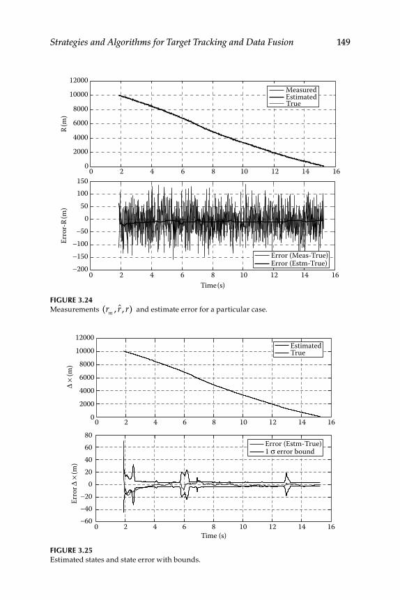
Strategies and Algorithms for Target Tracking and Data Fusion 149

FIGURE 3.24 Measurements (rm , r, r) and estimate error for a particular case.

0 2 4 6 8 10 12 14 160

2000

4000

6000

8000

10000

12000

R(m

)

0 2 4 6 8 10 12 14 16-200-150-100

-500

50100150

Time(s)

Erro

r-R(m

)

MeasuredEstimated True

Error (Estm-True)Error (Meas-True)

FIGURE 3.25 Estimated states and state error with bounds.

0 2 4 6 8 10 12 14 1602000400060008000

1000012000

0 2 4 6 8 10 12 14 16−60−40−20

020406080

TrueEstimated

Time (s)

1 σ error boundError (Estm-True)

Δ ×

(m)

Erro

rΔ ×

(m)

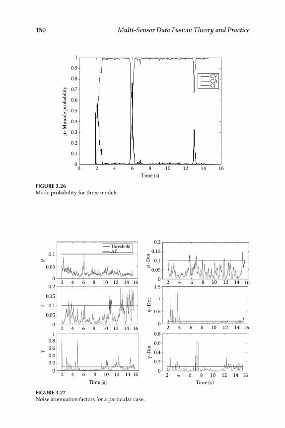
150 Multi-Sensor Data Fusion: Theory and Practice

FIGURE 3.26 Mode probability for three models.

0 2 4 6 8 10 12 14 160

0.1

0.2

0.3

0.4

0.5

0.6

0.7

0.8

0.9

1μ

-Mm

ode p

roba

bilit

y

CVCACJ

Time (s)

FIGURE 3.27 Noise attenuation factors for a particular case.

0.05

0 2 4 6 8 10 12 14 16 2 4 6 8 10 12 14 16

2 4 6 8 10 12 14 16

2 4 6 8 10Time (s)Time (s)

12 14 16

2 4 6 8 10 12 14 16

2 4 6 8 10 12 14 16

0.1

0.150.1

0.050

00.20.40.6

0.8

φγ

ρ

ρ-D

otφ-

Dot

γ-D

ot

1

0.2

0.15

1.5

1

0.5

0

0.80.60.40.2

0

0.10.05

0

0.2ThresholdAF

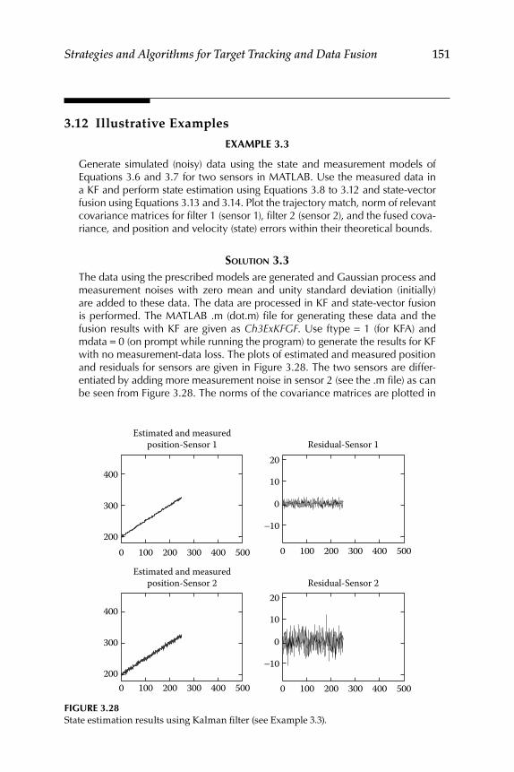
Strategies and Algorithms for Target Tracking and Data Fusion 151

3.12 Illustrative Examples

EXAMPLE 3.3

Generate simulated (noisy) data using the state and measurement models of Equations 3.6 and 3.7 for two sensors in MATLAB. Use the measured data in a KF and perform state estimation using Equations 3.8 to 3.12 and state-vector fusion using Equations 3.13 and 3.14. Plot the trajectory match, norm of relevant covariance matrices for fi lter 1 (sensor 1), fi lter 2 (sensor 2), and the fused cova-riance, and position and velocity (state) errors within their theoretical bounds.

SOLUTION 3.3 The data using the prescribed models are generated and Gaussian process and measurement noises with zero mean and unity standard deviation (initially) are added to these data. The data are processed in KF and state-vector fusion is performed. The MATLAB .m (dot.m) fi le for generating these data and the fusion results with KF are given as Ch3ExKFGF . Use ftype = 1 (for KFA) and mdata = 0 (on prompt while running the program) to generate the results for KF with no measurement-data loss. The plots of estimated and measured position and residuals for sensors are given in Figure 3.28. The two sensors are differ-entiated by adding more measurement noise in sensor 2 (see the .m fi le) as can be seen from Figure 3.28. The norms of the covariance matrices are plotted in

FIGURE 3.28 State estimation results using Kalman fi lter (see Example 3.3).

200

300

400

200

300

400

Estimated and measuredposition-Sensor 1

0 100 200 300 400 500

0 100 200 300 400 500

0 100 200 300 400 500

−10

0

10

20

0 100 200 300 400 500

−10

0

10

20

Residual-Sensor 1

Estimated and measuredposition-Sensor 2 Residual-Sensor 2

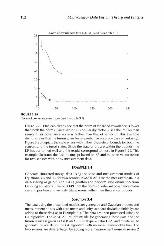
152 Multi-Sensor Data Fusion: Theory and Practice

Figure 3.29. One can clearly see that the norm of the fused covariance is lower than both the norms. Since sensor 2 is noisier (by factor 3; see the .m fi le) than sensor 1, its covariance norm is higher than that of sensor 1. This example demonstrates that the fusion gives better predictive accuracy (less uncertainty). Figure 3.30 depicts the state errors within their theoretical bounds for both the sensors and the fused states. Since the state errors are within the bounds, the KF has performed well and the results correspond to those in Figure 3.29. This example illustrates the fusion concept based on KF and the state-vector fusion for two sensors with noisy measurement data.

EXAMPLE 3.4

Generate simulated (noisy) data using the state and measurement models of Equations 3.6 and 3.7 for two sensors in MATLAB. Use the measured data in a data-sharing or gain-fusion (GF) algorithm and perform state estimation-cum-DF using Equations 3.142 to 3.149. Plot the norms of relevant covariance matri-ces and position and velocity (state) errors within their theoretical bounds.

SOLUTION 3.4 The data using the prescribed models are generated and Gaussian process and measurement noises with zero mean and unity standard deviation (initially) are added to these data as in Example 3.3. The data are then processed using the GF algorithm. The MATLAB .m (dot.m) fi le for generating these data and the fusion results is given as Ch3ExKFGF . Use ftype = 2 (for GFA) and mdata = 0 to generate the results for the GF algorithm with no measurement-data loss. The two sensors are differentiated by adding more measurement noise in sensor 2

FIGURE 3.29 Norm of covariance matrices (see Example 3.3).

0 50 100 150 200 2500

0.1

0.2

0.3

0.4

0.5

0.6

0.7

0.8Norm of covariances for F1(.), F2(-) and fusion filter(-.)

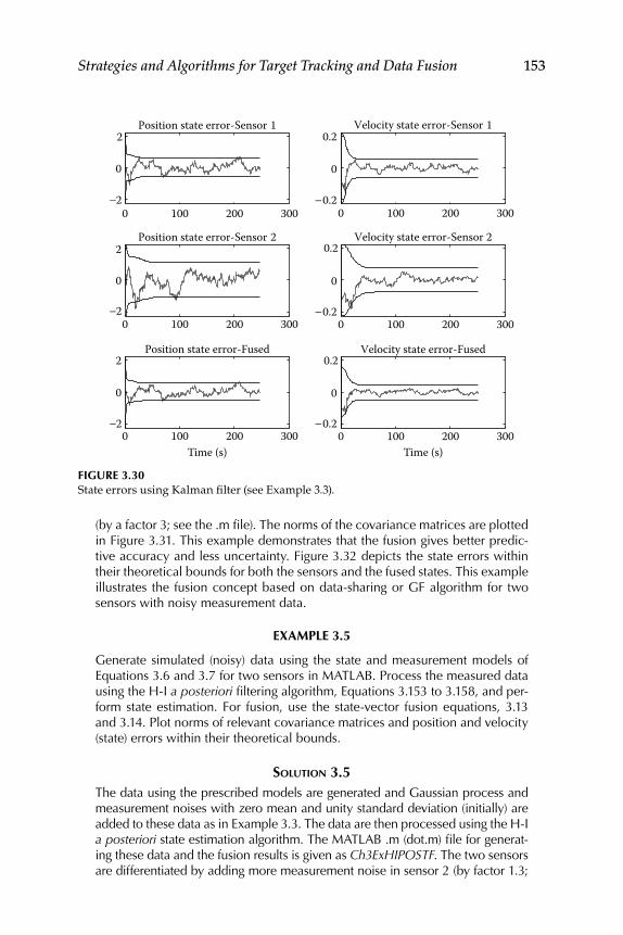
Strategies and Algorithms for Target Tracking and Data Fusion 153

(by a factor 3; see the .m fi le). The norms of the covariance matrices are plotted in Figure 3.31. This example demonstrates that the fusion gives better predic-tive accuracy and less uncertainty. Figure 3.32 depicts the state errors within their theoretical bounds for both the sensors and the fused states. This example illustrates the fusion concept based on data-sharing or GF algorithm for two sensors with noisy measurement data.

EXAMPLE 3.5

Generate simulated (noisy) data using the state and measurement models of Equations 3.6 and 3.7 for two sensors in MATLAB. Process the measured data using the H-I a posteriori fi ltering algorithm, Equations 3.153 to 3.158, and per-form state estimation. For fusion, use the state-vector fusion equations, 3.13 and 3.14. Plot norms of relevant covariance matrices and position and velocity (state) errors within their theoretical bounds.

SOLUTION 3.5 The data using the prescribed models are generated and Gaussian process and measurement noises with zero mean and unity standard deviation (initially) are added to these data as in Example 3.3. The data are then processed using the H-I a posteriori state estimation algorithm. The MATLAB .m (dot.m) fi le for generat-ing these data and the fusion results is given as Ch3ExHIPOSTF . The two sensors are differentiated by adding more measurement noise in sensor 2 (by factor 1.3;

FIGURE 3.30 State errors using Kalman fi lter (see Example 3.3).

0 100 200 300 0 100 200 300

0 100 200 300

0 100 200 300

0 100 200 300

0 100 200 300

−2

0

2Position state error-Sensor 1

−0.2

0

0.2Velocity state error-Sensor 1

−2

0

2Position state error-Sensor 2

−0.2

0

0.2Velocity state error-Sensor 2

−2

0

2

Time (s)

Position state error-Fused

−0.2

0

0.2

Time (s)

Velocity state error-Fused

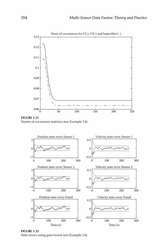
154 Multi-Sensor Data Fusion: Theory and Practice

FIGURE 3.31 Norms of covariance matrices (see Example 3.4).

0 50 100 150 200 2500.06

0.07

0.08

0.09

0.1

0.11

0.12

0.13Norm of covariances for F1(.), F2(-) and fusion filter(-.)

FIGURE 3.32 State errors using gain-fusion (see Example 3.4).

0 100 200 300 0 100 200 300

0 100 200 300

0 100 200 300

0 100 200 300

0 100 200 300

−2

0

2Position state error-Sensor 1

−0.2

0

0.2Velocity state error-Sensor 1

−2

0

2Position state error-Sensor 2

−0.2

0

0.2Velocity state error-Sensor 2

−2

0

2

Time (s)

Position state error-Fused

−0.2

0

0.2

Time (s)

Velocity state error-Fused

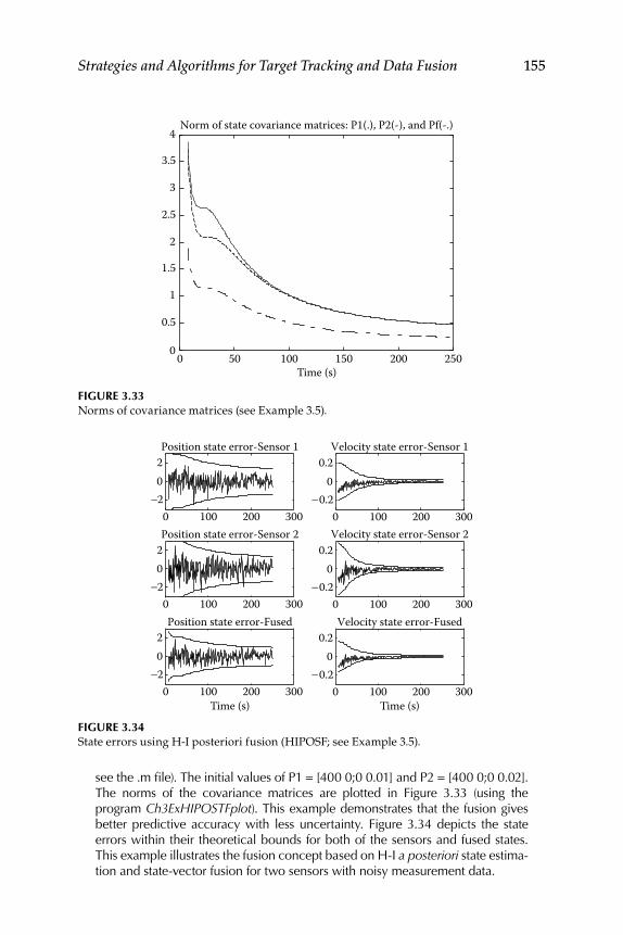
Strategies and Algorithms for Target Tracking and Data Fusion 155

see the .m fi le). The initial values of P1 = [400 0;0 0.01] and P2 = [400 0;0 0.02]. The norms of the covariance matrices are plotted in Figure 3.33 (using the program Ch3ExHIPOSTFplot ). This example demonstrates that the fusion gives better predictive accuracy with less uncertainty. Figure 3.34 depicts the state errors within their theoretical bounds for both of the sensors and fused states. This example illustrates the fusion concept based on H-I a posteriori state estima-tion and state-vector fusion for two sensors with noisy measurement data.

FIGURE 3.33 Norms of covariance matrices (see Example 3.5).

0 50 100 150 200 2500

0.5

1

1.5

2

2.5

3

3.5

4

Time (s)

Norm of state covariance matrices: P1(.), P2(-), and Pf(-.)

FIGURE 3.34 State errors using H-I posteriori fusion (HIPOSF; see Example 3.5).

0 100 200 3000 100 200 300

−202Position state error-Sensor 1

−0.20

0.2Velocity state error-Sensor 1

−202Position state error-Sensor 2

−0.20

0.2Velocity state error-Sensor 2

−202

Time (s)

Position state error-Fused

−0.20

0.2

Time (s)

Velocity state error-Fused

0 100 200 3000 100 200 300

0 100 200 3000 100 200 300

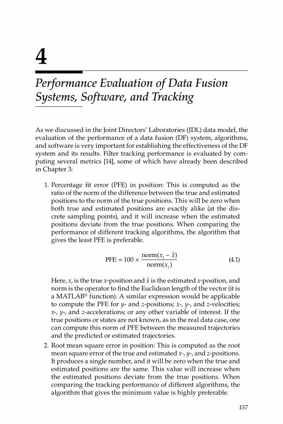
157

4 Performance Evaluation of Data Fusion Systems, Software, and Tracking

As we discussed in the Joint Directors’ Laboratories (JDL) data model, the evaluation of the performance of a data fusion (DF) system, algorithms, and software is very important for establishing the effectiveness of the DF system and its results. Filter tracking performance is evaluated by com-puting several metrics [14], some of which have already been described in Chapter 3:

1. Percentage fi t error (PFE) in position: This is computed as the ratio of the norm of the difference between the true and estimated positions to the norm of the true positions. This will be zero when both true and estimated positions are exactly alike (at the dis-crete sampling points), and it will increase when the estimated positions deviate from the true positions. When comparing the performance of different tracking algorithms, the algorithm that gives the least PFE is preferable.

PFE = 100 ×

norm(xt − x)

norm(xt ) (4.1)

Here, xt is the true x -position and x is the estimated x -position, and norm is the operator to fi nd the Euclidean length of the vector (it is a MATLAB® function). A similar expression would be applicable to compute the PFE for y - and z -positions; x -, y -, and z -velocities; x -, y -, and z -accelerations; or any other variable of interest. If the true positions or states are not known, as in the real data case, one can compute this norm of PFE between the measured trajectories and the predicted or estimated trajectories.

2. Root mean square error in position: This is computed as the root mean square error of the true and estimated x -, y -, and z -positions. It produces a single number, and it will be zero when the true and estimated positions are the same. This value will increase when the estimated positions deviate from the true positions. When comparing the tracking performance of different algorithms, the algorithm that gives the minimum value is highly preferable.

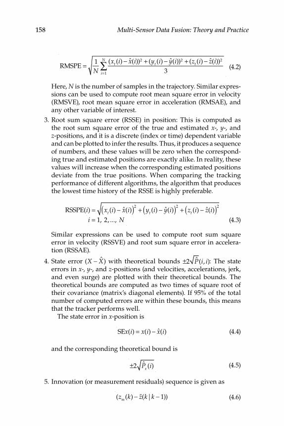
158 Multi-Sensor Data Fusion: Theory and Practice

RMSPE = 1

N(xt (i) − x(i))2 + (yt (i) − y(i))2 + (zt (i) − z(i))2

3i=1

N

∑

(4.2)

Here, N is the number of samples in the trajectory. Similar expres-sions can be used to compute root mean square error in velocity (RMSVE), root mean square error in acceleration (RMSAE), and any other variable of interest.

3. Root sum square error (RSSE) in position: This is computed as the root sum square error of the true and estimated x -, y -, and z -positions, and it is a discrete (index or time) dependent variable and can be plotted to infer the results. Thus, it produces a sequence of numbers, and these values will be zero when the correspond-ing true and estimated positions are exactly alike. In reality, these values will increase when the corresponding estimated positions deviate from the true positions. When comparing the tracking performance of different algorithms, the algorithm that produces the lowest time history of the RSSE is highly preferable.

RSSPE(i) = xt (i) − x(i)( )2+ yt (i) − y(i)( )2

+ zt (i) − z(i)( )2

i = 1, 2, ..., N (4.3)

Similar expressions can be used to compute root sum square error in velocity (RSSVE) and root sum square error in accelera-tion (RSSAE).

4. State error (X − X) with theoretical bounds ±2 P(i, i): The state errors in x -, y -, and z -positions (and velocities, accelerations, jerk, and even surge) are plotted with their theoretical bounds. The theoretical bounds are computed as two times of square root of their covariance (matrix’s diagonal elements). If 95% of the total number of computed errors are within these bounds, this means that the tracker performs well.

The state error in x -position is

SEx(i) = x(i) − x(i) (4.4)

and the corresponding theoretical bound is

±2 Px (i) (4.5)

5. Innovation (or measurement residuals) sequence is given as

(zm(k) − %z(k|k − 1)) (4.6)

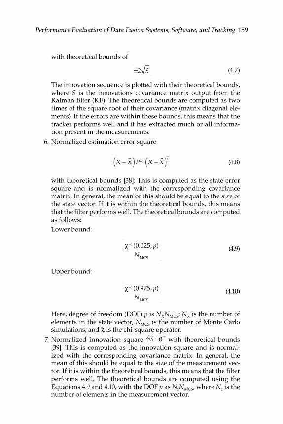
Performance Evaluation of Data Fusion Systems, Software, and Tracking 159

with theoretical bounds of

±2 S (4.7)

The innovation sequence is plotted with their theoretical bounds, where S is the innovations covariance matrix output from the Kalman fi lter (KF). The theoretical bounds are computed as two times of the square root of their covariance (matrix diagonal ele-ments). If the errors are within these bounds, this means that the tracker performs well and it has extracted much or all informa-tion present in the measurements.

6. Normalized estimation error square

X − X( )P−1 X − X( )T

(4.8)

with theoretical bounds [38]: This is computed as the state error square and is normalized with the corresponding covariance matrix. In general, the mean of this should be equal to the size of the state vector. If it is within the theoretical bounds, this means that the fi lter performs well. The theoretical bounds are computed as follows:

Lower bound:

χ−1(0.025, p)

NMCS

(4.9)

Upper bound:

χ−1(0.975, p)

NMCS

(4.10)

Here, degree of freedom (DOF) p is NXNMCS; NX is the number of elements in the state vector, NMCS is the number of Monte Carlo simulations, and χ is the chi-square operator.

7. Normalized innovation square ϑS−1ϑT with theoretical bounds [39]: This is computed as the innovation square and is normal-ized with the corresponding covariance matrix. In general, the mean of this should be equal to the size of the measurement vec-tor. If it is within the theoretical bounds, this means that the fi lter performs well. The theoretical bounds are computed using the Equations 4.9 and 4.10, with the DOF p as NzNMCS, where Nz is the number of elements in the measurement vector.

160 Multi-Sensor Data Fusion: Theory and Practice

4.1 Real-Time Flight Safety Expert System Strategy

A part of any multisensor tracking system, the fl ight test range requires a comprehensive planning of fl ight tests and preparation for test evalu-ation, while keeping the objectives and test-vehicle dynamics in mind. The evaluation process stems from the proposition of the range user and the intention of the test after the submission of the following fl ight vehi-cle information [69]: (1) fl ight objectives, (2) details of fl ight vehicle and fl ight dynamics, (3) instrumentation support needed, (4) measurement of parameters required, and (5) information on various failure mode studies carried out by the design and simulation groups.

Such a test launch of a fl ight vehicle is essentially monitored in real time with the help of various tracking sensors. The sensor data are supplied to the range safety offi cer (RSO) at the fl ight test range facility through the central computer after processing. Many test ranges use the sensor data available in real time to process and present the tracking trajectory indi-vidually to the RSO. Thus, there will be a number of trajectories, one from each sensor, which monitor the fl ight of a single vehicle (after multiplexed or concurrent processing in the central computer). A comparison of the tra-jectories is made using the safety background charts that are generated on the basis of extensive failure mode analysis of the fl ight vehicle, keeping in mind the topographical limitations of the range in relation to its surround-ings. It is very diffi cult for the RSO to assess the real-time fl ight vehicle position from the multiple trajectories presented by the sensors. She or he has to arrive at an appropriate decision almost instantaneously, which is very critical because of (1) the severity of the risk due to the errant fl ight vehicle, including uncertainty about its impact point, and (2) the very lim-ited time (2−3 seconds) available for the range safety offi ce to react.

Any human error or mistake in such crucial decision making could lead to the loss of lives and property. Humans’ subjective judgment could be erroneous due to various conditions and their state of mind: mental fatigue, biased decisions, slow reactions, memory loss, mistakes in judgment, and so on. Total dependence on a human safety offi cer for such a crucial judg-ment on termination (or otherwise) of fl ight vehicle, which could create unwarranted loss due wrong or delayed decisions, should always be ques-tioned. The capability of parallel processing or high-speed computer pro-cessors, the accessibility of huge amounts of memory, and the evolution of DF philosophy have opened up new avenues to meet the diffi culties faced by a human safety offi ce in a fl ight test range. The computation of trajecto-ries of the vehicle from a number of sensor data streams in real time, and then fusing these trajectories, aids the RSO to a great extent and reduces his or her workload. Thus, the ranges in the world are trying best to uti-lize such a philosophy and arrive at better decision making in order to

Performance Evaluation of Data Fusion Systems, Software, and Tracking 161

overcome the weak points of human psychology. The test range-tracking sensors are generally deployed and distributed over a large area along a long coastline or a range on land and in sea, and in some cases from a satellite or aircraft to cover various phases of the fl ight path trajectory. The range-tracking sensors used for target tracking are electro-optical transducers (EOTs), infrared (IR) trackers, laser rangers, charge-coupled devices (CCD) cameras, Doppler radar, beacon radar, and telemetry track-ers. Characterization of each measurement channel (Section 3.2) is a very important task, involving data collection from postfl ight records or by conducting helicopter or aircraft trial sorties over the range area.

4.1.1 Autodecision Criteria

The data processing system should have certain processing capabilities to ensure accuracy, reliability, and a fast response [69]: (1) validation cri-teria to fi x up data acceptability; (2) a dynamic tracking fi lter to estimate the target trajectory from the noisy measurements; (3) a multisensor DF (MSDF) to obtain fused trajectory for decision making; (4) an expert rule processor to determine the logic–based on the knowledge bank; (5) an inference engine to select the best among the alternative decisions; and (6) a display scheme to present the fi nal decision. After processing the data in KF, the system should combine the data at two or three levels to achieve one representative trajectory of the vehicle for fl ight safety decision mak-ing. In the next level of fusion, expert system−based decision architecture is used to give a fi nal decision for fl ight safety.

4.1.2 Objective of a Flight Test Range

The main role of a fl ight test range is to undertake a fl ight test and evaluate several weapons systems under development such as guided weapon sys-tems, unguided rocket systems, unmanned aerial vehicles, warhead test vehicles, and special aerial delivery systems. Some of the typical aspects need to be defi ned, such as suitable selection of sensor site, accurate sur-vey and deployment of tracking sensors to ensure full coverage of the trajectory from launch to impact, calibration of tracking sensors, range tracking network validation, real-time range safety monitoring and deci-sion making for safe launch, reliable tracking and processing system, data accuracy and acceptance criteria, data security, storage and maintenance, and video data processing and analysis.

4.1.3 Scenario of the Test Range

Trajectory tracking sensors are deployed over a vast area along the coast and downrange and are connected to the central computer through a reliable communication link.

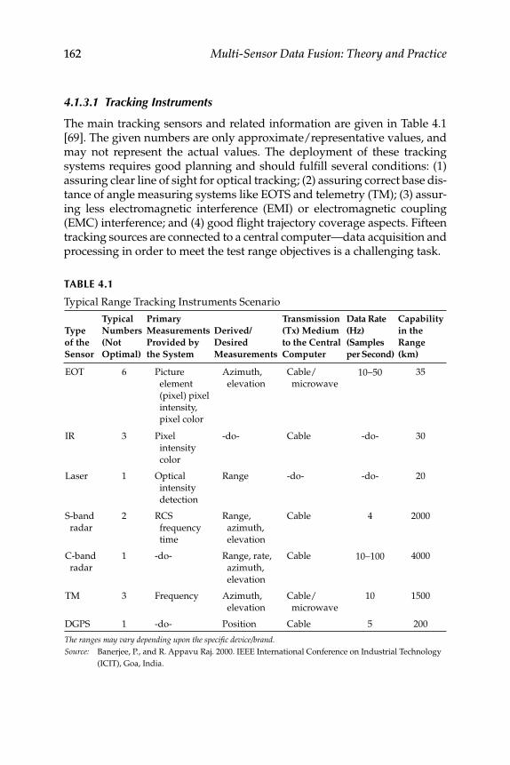
162 Multi-Sensor Data Fusion: Theory and Practice

4.1.3.1 Tracking Instruments

The main tracking sensors and related information are given in Table 4.1 [69]. The given numbers are only approximate/representative values, and may not represent the actual values. The deployment of these tracking systems requires good planning and should fulfi ll several conditions: (1) assuring clear line of sight for optical tracking; (2) assuring correct base dis-tance of angle measuring systems like EOTS and telemetry (TM); (3) assur-ing less electromagnetic interference (EMI) or electromagnetic coupling (EMC) interference; and (4) good fl ight trajectory coverage aspects. Fifteen tracking sources are connected to a central computer—data acquisition and processing in order to meet the test range objectives is a challenging task.

TABLE 4.1

Typical Range Tracking Instruments Scenario

Type

of the

Sensor

Typical

Numbers

(Not

Optimal)

Primary

Measurements

Provided by

the System

Derived/

Desired

Measurements

Transmission

(Tx) Medium

to the Central

Computer

Data Rate

(Hz)

(Samples

per Second)

Capability

in the

Range

(km)

EOT 6 Picture

element

(pixel) pixel

intensity,

pixel color

Azimuth,

elevation

Cable/

microwave10−50 35

IR 3 Pixel

intensity

color

-do- Cable -do- 30

Laser 1 Optical

intensity

detection

Range -do- -do- 20

S-band

radar

2 RCS

frequency

time

Range,

azimuth,

elevation

Cable 4 2000

C-band

radar

1 -do- Range, rate,

azimuth,

elevation

Cable 10−100 4000

TM 3 Frequency Azimuth,

elevation

Cable/

microwave

10 1500

DGPS 1 -do- Position Cable 5 200

The ranges may vary depending upon the specifi c device/brand.Source: Banerjee, P., and R. Appavu Raj. 2000. IEEE International Conference on Industrial Technology

(ICIT), Goa, India.

Performance Evaluation of Data Fusion Systems, Software, and Tracking 163

4.1.3.2 Data Acquisition

Missile coordinate data from the tracking instruments is transmitted to the central computer through RS-232 C digital interface, connected through a modem to an audio frequency-dedicated line. The computer also acquires central and countdown timing data through parallel input interfaces. The raw data from tracking instruments are validated using certain criteria [69]: (1) communication error check (longitudinal redundancy check), (2) tracking station check, and (3) validation by 3s criteria. Other criteria are also applied: (1) systematic error correction, (2) refraction error correction, (3) correction due to earth curvature, and (4) correction due to transmission delay. Other processing tasks are (1) tra-jectory computation, (2) fi ltering, (3) coordinate conversion, (4) computer designate mode data T x , (5) range safety computation, and (6) display task activation or graphics.

4.1.3.3 Decision Display System

This system consists of two sets of workstations, which receive current state vector, and impact footprints of fl ight vehicle from multiple track sources superimposed on destruct contours. The decision to terminate the fl ight vehicle is based on the following: (1) when the real-time trajectory of the fl ight vehicle parallels one of the destruct-contours; and (2) when the impact footprint intersects with the shore line. The decision is further reinforced using missile health parameters displayed on the PC system. The expert-based decision support system wherein the machine processes the source data and displays the fl ight safety action required during real time is established. The two levels of fusion used are (1) fi rst-level fusion based on priority and fusion of similar sensors using the MSDF method; and (2) decision-level fusion based on voting, expert decision support sys-tem (DSS).

4.1.4 Multisensor Data Fusion System

Sensors are normally subjected to external noise, internal malfunction-ing, and mechanical failures. To ensure that a system receives a realistic view of its environment, it is necessary to combine the readings of two or more sensors. This process is benefi cial to human decision making, as the decision is made under time constraints and is based on a large amount of sensor information.

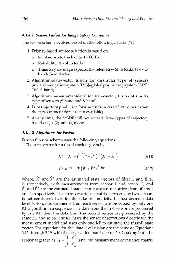
164 Multi-Sensor Data Fusion: Theory and Practice

4.1.4.1 Sensor Fusion for Range Safety Computer

The fusion scheme evolved based on the following criteria [69]:

1. Priority-based source selection is based on

a. Most accurate track data: I - EOTS

b. Reliability: II - Skin Radar

c. Trajectory coverage aspects: III- Telemetry- Skin Radar } IV - C- band- Skin Radar

2. Algorithm/state-vector fusion for dissimilar type of sensors (inertial navigation system [INS]−global positioning system [GPS], TM−S-band)

3. Algorithm/measurement-level (or state-vector) fusion of similar type of sensors (S-band and S-band)

4. Pure trajectory prediction for 4 seconds in case of track loss (when the measurement data are not available)

5. At any time, the MSDF will not exceed three types of trajectory based on (1), (2), and (3) alone.

4.1.4.2 Algorithms for Fusion

Fusion fi lter or scheme uses the following equations: The state vector for a fused track is given by

X f = X1 + P1 P1 + P2( )−1

X 2 − X1( ) (4.11)

P f = P1 − P1 P1 + P2( )−1

P1T

(4.12)

where, X1 and X 2 are the estimated state vectors of fi lter 1 and fi lter 2, respectively, with measurements from sensor 1 and sensor 2, and P1 and P 2 are the estimated state error covariance matrices from fi lters 1 and 2, respectively. The cross-covariance matrix between any two sensors is not considered here for the sake of simplicity. In measurement data level fusion, measurements from each sensor are processed by only one KF algorithm in a sequence. The data from the fi rst sensor are processed by one KF, then the data from the second sensor are processed by the same KF and so on. The KF fuses the sensor observations directly via the measurement model and uses only one KF to estimate the (fused) state vector. The equations for this data level fusion are the same as Equations 3.15 through 3.19, with the observation matrix being 2 × 2, taking both the

sensor together as H =1 0

1 0

⎡

⎣⎢

⎤

⎦⎥ , and the measurement covariance matrix

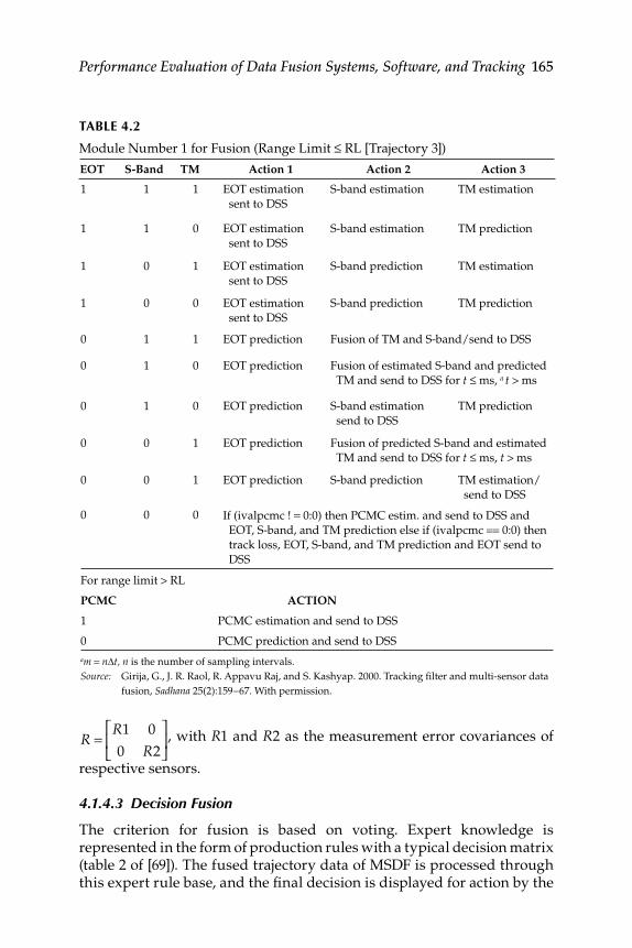
Performance Evaluation of Data Fusion Systems, Software, and Tracking 165

R =R1 0

0 R2

⎡

⎣⎢

⎤

⎦⎥, with R 1 and R 2 as the measurement error covariances of

respective sensors.

4.1.4.3 Decision Fusion

The criterion for fusion is based on voting. Expert knowledge is represented in the form of production rules with a typical decision matrix (table 2 of [69]). The fused trajectory data of MSDF is processed through this expert rule base, and the fi nal decision is displayed for action by the

TABLE 4.2

Module Number 1 for Fusion (Range Limit ≤ RL [Trajectory 3])

EOT S-Band TM Action 1 Action 2 Action 3

1 1 1 EOT estimation

sent to DSS

S-band estimation TM estimation

1 1 0 EOT estimation

sent to DSS

S-band estimation TM prediction

1 0 1 EOT estimation

sent to DSS

S-band prediction TM estimation

1 0 0 EOT estimation

sent to DSS

S-band prediction TM prediction

0 1 1 EOT prediction Fusion of TM and S-band/send to DSS

0 1 0 EOT prediction Fusion of estimated S-band and predicted

TM and send to DSS for t ≤ ms, a t > ms

0 1 0 EOT prediction S-band estimation

send to DSS

TM prediction

0 0 1 EOT prediction Fusion of predicted S-band and estimated

TM and send to DSS for t ≤ ms, t > ms

0 0 1 EOT prediction S-band prediction TM estimation/

send to DSS

0 0 0 If (ivalpcmc ! = 0:0) then PCMC estim. and send to DSS and

EOT, S-band, and TM prediction else if (ivalpcmc == 0:0) then

track loss, EOT, S-band, and TM prediction and EOT send to

DSS

For range limit > RL

PCMC ACTION

1 PCMC estimation and send to DSS

0 PCMC prediction and send to DSS

am = nDt, n is the number of sampling intervals.

Source: Girija, G., J. R. Raol, R. Appavu Raj, and S. Kashyap. 2000. Tracking fi lter and multi-sensor data

fusion, Sadhana 25(2):159−67. With permission.

166 Multi-Sensor Data Fusion: Theory and Practice

RSO. The software is run in Microsoft Windows under the Visual C++ platform. Further related results are discussed in Section 4.2.

4.2 Multisensor Single-Target Tracking

The multisensor single-target (MSST) strategy is validated using postfl ight data. The state and measurement models used are

xj+1

= φ j , j+1xj + Gwj (4.13)

zj = Hxj + vj (4.14)

with the associated state transition matrix as

φ =1 Δt Δt2/2

0 1 Δt

0 0 1

⎡

⎣

⎢⎢⎢

⎤

⎦

⎥⎥⎥

(4.15)

Here, H = [1 0 0] is the measurement model, and state vector x has position, velocity, and acceleration as its components. The KF is implemented in the factorized form for this application. The U-D fi lter (Section 3.2) is developed in C language and implemented on Unix-based Alpha-DEC computer. It is validated using simulated trajectory data and also real-fl ight data.

4.2.1 Hierarchical Multisensor Data Fusion Architecture and Fusion Scheme

A hierarchical MSDF architecture adopted for a typical fl ight test range equipped with several types of sensors for tracking a fl ight vehicle is given in Figure 4.1 [70]. This obtains three sets of fused positions ( x , y , z ) and corresponding velocity state information to a DSS (as the user’s facility or in the control room of the range facility). The data from two ground-based radars (azimuth, elevation, and range) are combined via polar-to- Cartesian (PTC) coordinate transformation, used in the individual U-D fi lters, and then fused to obtain Trajectory 1 (Traj1/ t , x , y , z , velocities in the three axes). Here, U is an upper triangular unitary matrix and D is a diagonal matrix. Trajectory 2 (Traj2) is generated by the fusion of INS ( t , x , y , z , and velocities) and GPS ( t , x , y , z ) data (received at the ground station) by using appropriate U-D fi lters and the fusion fi lter. The angular data from the TM channels that measure only the azimuth (f) and elevation (q) are combined using least-squares (LS) method to generate position information ( t , x , y , z ). The azimuth and elevation data from EOTs are

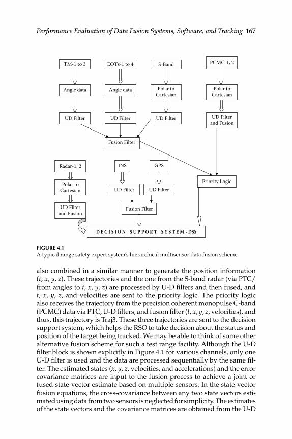
Performance Evaluation of Data Fusion Systems, Software, and Tracking 167

also combined in a similar manner to generate the position information ( t , x , y , z ). These trajectories and the one from the S-band radar (via PTC/from angles to t , x , y , z ) are processed by U-D fi lters and then fused, and t , x , y , z , and velocities are sent to the priority logic. The priority logic also receives the trajectory from the precision coherent monopulse C-band (PCMC) data via PTC, U-D fi lters, and fusion fi lter ( t , x , y , z , velocities), and thus, this trajectory is Traj3. These three trajectories are sent to the decision support system, which helps the RSO to take decision about the status and position of the target being tracked. We may be able to think of some other alternative fusion scheme for such a test range facility. Although the U-D fi lter block is shown explicitly in Figure 4.1 for various channels, only one U-D fi lter is used and the data are processed sequentially by the same fi l-ter. The estimated states ( x , y , z , velocities, and accelerations) and the error covariance matrices are input to the fusion process to achieve a joint or fused state-vector estimate based on multiple sensors. In the state- vector fusion equations, the cross-covariance between any two state vectors esti-mated using data from two sensors is neglected for simplicity. The estimates of the state vectors and the covariance matrices are obtained from the U-D

FIGURE 4.1 A typical range safety expert system’s hierarchical multisensor data fusion scheme.

TM-1 to 3 EOTs-1 to 4 S-Band PCMC-1, 2

Angle data Angle data Polar toCartesian

UD Filter UD Filter UD Filter UD Filterand Fusion

Fusion Filter

Priority Logic

Radar-1, 2

UD FilterUD Filter

INS

Polar toCartesian

GPS

Fusion FilterUD Filterand Fusion

D E C I S I O N S U P P O R T S Y S T E M - DSS

Polar toCartesian

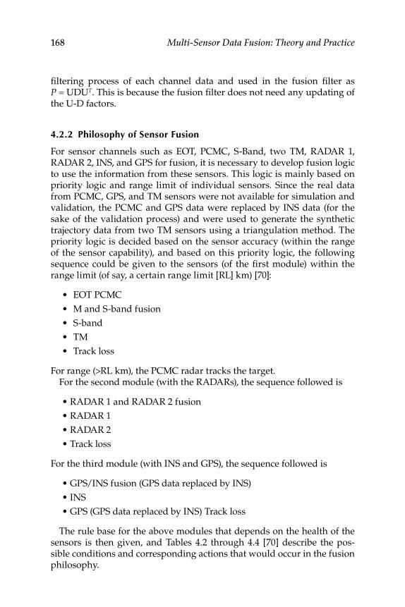
168 Multi-Sensor Data Fusion: Theory and Practice

fi ltering process of each channel data and used in the fusion fi lter as P = UDUT. This is because the fusion fi lter does not need any updating of the U-D factors.

4.2.2 Philosophy of Sensor Fusion

For sensor channels such as EOT, PCMC, S-Band, two TM, RADAR 1, RADAR 2, INS, and GPS for fusion, it is necessary to develop fusion logic to use the information from these sensors. This logic is mainly based on priority logic and range limit of individual sensors. Since the real data from PCMC, GPS, and TM sensors were not available for simulation and validation, the PCMC and GPS data were replaced by INS data (for the sake of the validation process) and were used to generate the synthetic trajectory data from two TM sensors using a triangulation method. The priority logic is decided based on the sensor accuracy (within the range of the sensor capability), and based on this priority logic, the following sequence could be given to the sensors (of the fi rst module) within the range limit (of say, a certain range limit [RL] km) [70]:

EOT PCMC •

M and S-band fusion •

S-band •

TM •

Track loss •

For range (>RL km), the PCMC radar tracks the target. For the second module (with the RADARs), the sequence followed is

• RADAR 1 and RADAR 2 fusion

• RADAR 1

• RADAR 2

• Track loss

For the third module (with INS and GPS), the sequence followed is

• GPS/INS fusion (GPS data replaced by INS)

• INS

• GPS (GPS data replaced by INS) Track loss

The rule base for the above modules that depends on the health of the sensors is then given, and Tables 4.2 through 4.4 [70] describe the pos-sible conditions and corresponding actions that would occur in the fusion philosophy.

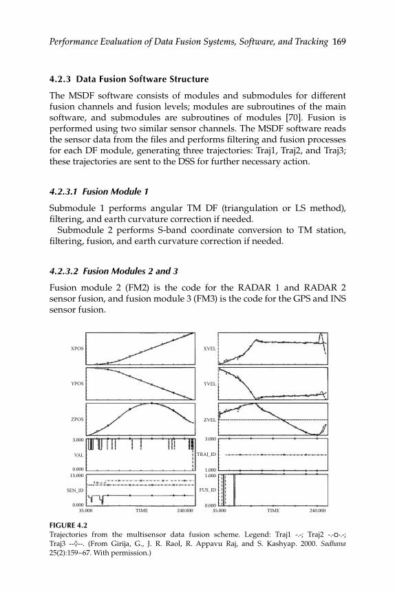
Performance Evaluation of Data Fusion Systems, Software, and Tracking 169

4.2.3 Data Fusion Software Structure

The MSDF software consists of modules and submodules for different fusion channels and fusion levels; modules are subroutines of the main software, and submodules are subroutines of modules [70]. Fusion is performed using two similar sensor channels. The MSDF software reads the sensor data from the fi les and performs fi ltering and fusion processes for each DF module, generating three trajectories: Traj1, Traj2, and Traj3; these trajectories are sent to the DSS for further necessary action.

4.2.3.1 Fusion Module 1

Submodule 1 performs angular TM DF (triangulation or LS method), fi ltering, and earth curvature correction if needed.

Submodule 2 performs S-band coordinate conversion to TM station, fi ltering, fusion, and earth curvature correction if needed.

4.2.3.2 Fusion Modules 2 and 3

Fusion module 2 (FM2) is the code for the RADAR 1 and RADAR 2 sensor fusion, and fusion module 3 (FM3) is the code for the GPS and INS sensor fusion.

FIGURE 4.2 Trajectories from the multisensor data fusion scheme. Legend: Traj1 -.-; Traj2 -.- -.-;

Traj3 --◊--. (From Girija, G., J. R. Raol, R. Appavu Raj, and S. Kashyap. 2000. Sadhana

25(2):159−67. With permission.)

XPOS

YPOS

ZPOS

3.000

VAL

0.00015.000

SEN_ID

0.00035.000 TIME 240.000

XVEL

YVEL

ZVEL

3.000

TRAJ_ID

1.0001.000

FUS_ID

0.00035.000 TIME 240.000

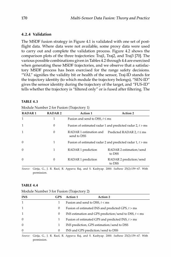
170 Multi-Sensor Data Fusion: Theory and Practice

4.2.4 Validation

The MSDF fusion strategy in Figure 4.1 is validated with one set of post-fl ight data. Where data were not available, some proxy data were used to carry out and complete the validation process. Figure 4.2 shows the comparison plots of the three trajectories: Traj1, Traj2, and Traj3 [70]. The various possible combinations given in Tables 4.2 through 4.4 are exercised when generating these MSDF trajectories, and we observe that a satisfac-tory MSDF process has been exercised for the range safety decisions. “VAL” signifi es the validity bit or health of the sensor, Traj-ID stands for the trajectory identity (to which module the trajectory belongs), “SEN-ID” gives the sensor identity during the trajectory of the target, and “FUS-ID” tells whether the trajectory is “fi ltered only” or is fused after fi ltering. The

TABLE 4.3

Module Number 2 for Fusion (Trajectory 1)

RADAR 1 RADAR 2 Action 1 Action 2

1 1 Fusion and send to DSS, t ≤ ms

1 0 Fusion of estimated radar 1 and predicted radar 2, t > ms

1 0 RADAR 1 estimation and

send to DSSPredicted RADAR 2, t ≤ ms

0 1 Fusion of estimated radar 2 and predicted radar 1, t > ms

0 1 RADAR 1 prediction RADAR 2 estimation/send

to DSS

0 0 RADAR 1 prediction RADAR 2 prediction/send

to DSS

Source: Girija, G., J. R. Raol, R. Appavu Raj, and S. Kashyap. 2000. Sadhana 25(2):159−67. With

permission.

TABLE 4.4

Module Number 3 for Fusion (Trajectory 2)

INS GPS Action 1 Action 2

1 1 Fusion and send to DSS, t < ms

1 0 Fusion of estimated INS and predicted GPS, t > ms

1 0 INS estimation and GPS prediction/send to DSS, t < ms

0 1 Fusion of estimated GPS and predicted INS, t > ms

0 1 INS prediction, GPS estimation/send to DSS

0 0 INS and GPS prediction/send to DSS

Source: Girija, G., J. R. Raol, R. Appavu Raj, and S. Kashyap. 2000. Sadhana 25(2):159−67. With

permission.

Performance Evaluation of Data Fusion Systems, Software, and Tracking 171

strategy and algorithms of Sections 4.1 and 4.2 have also been further evaluated at the actual test range.

4.3 Tracking of a Maneuvering Target—Multiple-Target

Tracking Using Interacting Multiple Model

Probability Data Association Filter and Fusion

The performance of interacting multiple model probability data associa-tion fi lters (IMMPDAF) for the estimation of multiple maneuvering target trajectories in clutter is investigated using simulated data, the targets being tracked by a single sensor. The scheme can be extended to more than one sensor, and evaluates the sensitivity of the fi lter to the choice of the mod-els and process noise covariance matrix values. The use of the IMMPDAF algorithm for the tracking and fusion of simulated data for four targets whose positions are measured by two sensors located at different spatial positions is also discussed in this section. Thus, the algorithm is evalu-ated for a multisensor multitarget scenario using the fusion method. The IMMPDAF gives a realistic confi dence in estimates during maneuvers and a low RSSPE during the nonmaneuvering phase of the targets.

4.3.1 Interacting Multiple Model Algorithm

The interactive multiple model (IMM) algorithm and related concepts [38,39,43,50,51,53] are versatile methods for adaptive state estimation in systems whose behavior changes with time, and which obey one of a fi nite number of models. Two or more models are run in concurrence (of course this is mainly true in the case of parallel computer-based implementa-tions) to achieve better performance of maneuvering targets. The features of IMM can be combined with probability data association fi lters (PDAF) to obtain the IMMPDAF algorithm. Figure 4.3 [71] depicts one cycle of a two-model IMMPDAF algorithm [50,51], which is applicable to single-sensor multitarget scenario, and can also be extended to multiple sensors. Figure 4.4 depicts the block schematic of the multisensor−multitarget (MSMT) fusion algorithm [71].

4.3.1.1 Automatic Track Formation

The objective of track initiation is to compute initial state estimates of all possible tracks along with the computations of the associated state covari-ance matrices. There is a possibility of false tracks being generating due to the presence of spurious measurements and multiple targets. The following technique to initiate a track based on a logic that requires M detections out of N scans in the gate can be used: A tentative track is formed on all two-measurement pairs with the expected motions of the targets.

172 Multi-Sensor Data Fusion: Theory and Practice

4.3.1.2 Gating and Data Association

After the formation of the track, the measurement screening is carried out using the procedure outlined in Chapter 3 (Equations 3.1 through 3.5) to determine potential candidates for corresponding tracks. The combined innovation sequence v is computed using the steps, as in the PDAF (see Section 3.4), which has two additional blocks (compared to nearest- neighbor KF [NNKF]/KF) for the computation of association probabilities bi(k) and combined innovations sequences v(k). If vi(k) corresponds to innovation on measurement i, then the merged innovation is given by

FIGURE 4.3 Interacting multiple models probability data association fi lter block diagram for two

models.

μi(k)

μi|j(k|k)

c 1,c 2

Λ1

++

Data fromSensorsTrack formation

Gating

Interactionand mixing

Filter 1 Filter 2

Update of modeprobabilities and

computationof mixing

probabilities

Estimation ofstates andcovariance

merging

Updateof states

Prediction ofstates/

covariancemerging

Output fused state estimatesand covariance

Transitionprobabilities

PDAF

Λ2

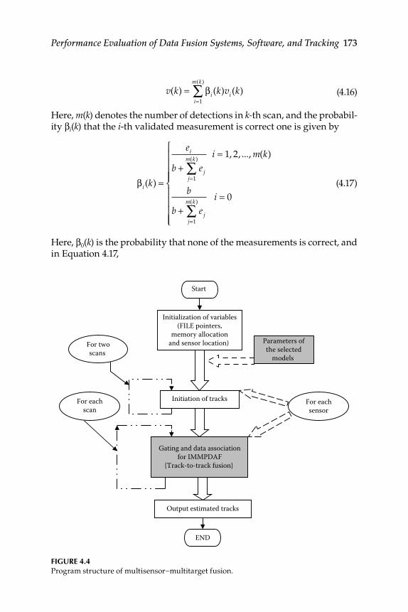
Performance Evaluation of Data Fusion Systems, Software, and Tracking 173

v(k) = βi (k)vi (k)

i=1

m(k )

∑

(4.16)

Here, m(k) denotes the number of detections in k- th scan, and the probabil-ity βi(k) that the i-th validated measurement is correct one is given by

βi(k) =

ei

b + e jj=1

m(k)

∑i = 1, 2, ..., m(k)

b

b + e jj=1

m(k)

∑i = 0

⎧

⎨

⎪⎪⎪⎪

⎩

⎪⎪⎪⎪

(4.17)

Here, β0(k) is the probability that none of the measurements is correct, and in Equation 4.17,

FIGURE 4.4 Program structure of multisensor−multitarget fusion.

Initialization of variables(FILE pointers,

memory allocationand sensor location)

Initiation of tracks

Output estimated tracks

END

For eachsensor

For eachscan

For twoscans

Gating and data associationfor IMMPDAF

{Track-to-track fusion}

Parameters ofthe selected

models

Start

174 Multi-Sensor Data Fusion: Theory and Practice

ei ≅ e

−1

2νi (k )'S(k )−1 νi (k ) (4.18)

b ≅ 2π

γ⎛⎝⎜

⎞⎠⎟

nz

2

m(k)cn2

−1(1 − PDPG )

PD (4.19)

Here, nz is the dimension of the measurement, cnz is the volume of the

unit hypersphere of dimensions (c1 = 2, c2 = π, c3 = 4π/3, and so on), and PG and PD represent the gate probability and probability of target detection. The computed βi(k) and v(k) are used to estimate the states and covariance matrices of the updating cycle. The resulting measurement used next in mode-conditioned fi ltering is computed with the following equation:

Z(k) = H %X

kk − 1

⎛⎝⎜

⎞⎠⎟

+ v(k) (4.20)

Here, %X(k / k − 1) is the predicted target state at k -th scan and is computed from the state and covariance prediction blocks (Figure 4.3).

4.3.1.3 Interaction and Mixing in Interactive Multiple Model Probabilistic Data Association Filter

This step uses the mixing probabilities μi|j (k − 1|k − 1) as weighting coeffi cients, the estimates of Xandi(k − 1|k − 1) and Pi(k − 1|k − 1) from the previous cycle are used to obtain the initial conditions X0j(k − 1|k − 1) and

P0j (k − 1|k − 1) for the mode-matched fi lters M1 and M2 of the present cycle. For all i, j ∈ M, the initial conditions for the fi lters are computed from the following equations:

X

0 j (k − 1|k − 1) = Xii=1

r

∑ (k − 1|k − 1)μ i|j (k − 1|k − 1)

(4.21)

P0 j (k − 1|k − 1) =

Pi (k − 1|k − 1)

+[{Xi (k − 1|k − 1) − X0 j (k − 1|k − 1)}

× {Xi (k − 1|k − 1) − X0 j (k − 1|k − 1)}T]

⎡

⎣

⎢⎢⎢⎢

⎤

⎦

⎥⎥⎥⎥

i=1

r

∑ μ i|j (k − 1|k − 1)

(4.22)

Here, mode-matched fi lters run as j = 1, … r; the models run as i = 1, … r; and r = 2 for the two-model IMM method.

4.3.1.4 Mode-Conditioned Filtering

With r parallel (though used in a sequential mode only!) mode-matched KFs, the states and covariance matrices are estimated using the normal prediction and update steps.

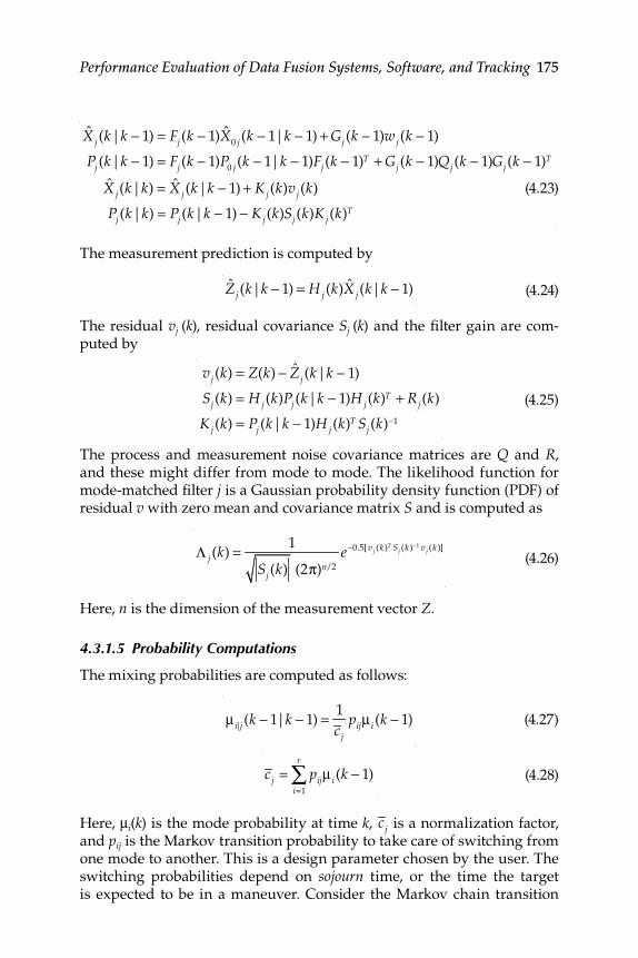
Performance Evaluation of Data Fusion Systems, Software, and Tracking 175

X j (k|k − 1) = Fj (k − 1)X0 j (k − 1|k − 1) + Gj (k − 1)wj (k − 1)

Pj (k|k − 1) = Fj (k − 1)P0 j (k − 1|k − 1)Fj (k − 1)T + Gj (k − 1)Qj (k − 1)Gj (k − 1)T

X j (k|k) = X j (k|k − 1) + Kj (k)vj (k)

Pj (k|k) = Pj (k|k − 1) − Kj (k)Sj (k)Kj (k)T

(4.23)

The measurement prediction is computed by

Zj (k|k − 1) = H j (k)X j (k|k − 1) (4.24)

The residual vj (k), residual covariance Sj (k) and the fi lter gain are com-puted by

vj (k) = Z(k) − Zj (k|k − 1)

Sj (k) = H j (k)Pj (k|k − 1)H j (k)T + Rj (k)

Kj (k) = Pj (k|k − 1)H j (k)T Sj (k)−1

(4.25)

The process and measurement noise covariance matrices are Q and R, and these might differ from mode to mode. The likelihood function for mode-matched fi lter j is a Gaussian probability density function (PDF) of residual v with zero mean and covariance matrix S and is computed as

Λ j (k) = 1

Sj (k) (2π)n/2

e−0.5[vj (k )T Sj (k )−1 vj (k )]

(4.26)

Here, n is the dimension of the measurement vector Z.

4.3.1.5 Probability Computations

The mixing probabilities are computed as follows:

μ i|j (k − 1|k − 1) = 1

cj

pijμ i (k − 1)

(4.27)

cj = pij

i=1

r

∑ μ i (k − 1)

(4.28)

Here, μi(k) is the mode probability at time k, cj is a normalization factor, and pij is the Markov transition probability to take care of switching from one mode to another. This is a design parameter chosen by the user. The switching probabilities depend on sojourn time, or the time the target is expected to be in a maneuver. Consider the Markov chain transition

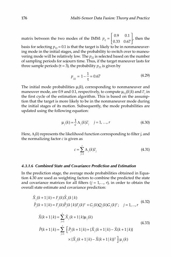
176 Multi-Sensor Data Fusion: Theory and Practice

matrix between the two modes of the IMM: pij =0.9 0.1

0.33 0.67

⎡

⎣⎢

⎤

⎦⎥ , then the

basis for selecting p12 = 0.1 is that the target is likely to be in nonmaneuver-ing mode in the initial stages, and the probability to switch over to maneu-vering mode will be relatively low. The p22 is selected based on the number of sampling periods for sojourn time. Thus, if the target maneuver lasts for three sample periods (τ = 3), the probability p22 is given by

p22= 1 − 1

τ= 0.67

(4.29)

The initial mode probabilities μi(k), corresponding to nonmaneuver and maneuver mode, are 0.9 and 0.1, respectively, to compute μi|j(k|k) and c–j in the fi rst cycle of the estimation algorithm. This is based on the assump-tion that the target is more likely to be in the nonmaneuver mode during the initial stages of its motion. Subsequently, the mode probabilities are updated using the following equation:

μ j (k) = 1

c Λ j (k)cj j = 1, …, r

(4.30)

Here, Λj(k) represents the likelihood function corresponding to fi lter j, and the normalizing factor c is given as

c = Λ j (k)cj

j=1

r

∑

(4.31)

4.3.1.6 Combined State and Covariance Prediction and Estimation

In the prediction stage, the average mode probabilities obtained in Equa-tion 4.30 are used as weighting factors to combine the predicted the state and covariance matrices for all fi lters (j = 1,…, r), in order to obtain the overall state estimate and covariance prediction:

%X j (k + 1|k) = Fj (k)X j (k|k)

%Pj (k + 1|k) = Fj (k)Pj (k|k)Fj (k)T + Gj (k)Qj (k)Gj (k)T ; j = 1, ..., r (4.32)

%X(k + 1|k) = %X j (k + 1|k)μ j (k)j=1

r

∑

%P(k + 1|k) = %Pj (k + 1|k) + { %X j (k + 1|k) − %X(k + 1|k)}⎡⎣j=1

r

∑

× { %X j (k + 1|k) − %X(k + 1|k)}T ⎤⎦ μ j (k)

(4.33)

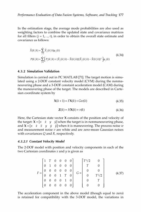
Performance Evaluation of Data Fusion Systems, Software, and Tracking 177

In the estimation stage, the average mode probabilities are also used as weighting factors to combine the updated state and covariance matrices for all fi lters (j = 1,…, r), in order to obtain the overall state estimate and covariance as follows:

X(k|k) = X j (k|k)μ j (k)j=1

r

∑

P(k|k) = Pj (k|k) + {X j (k|k) − X(k|k)}{X j (k|k) − X(k|k)}T⎡⎣ ⎤⎦j=1

r

∑ μ j (k)

(4.34)

4.3.2 Simulation Validation

Simulation is carried out in PC MATLAB [71]. The target motion is simu-lated using a 2-DOF constant velocity model (CVM) during the nonma-neuvering phase and a 3-DOF constant acceleration model (CAM) during the maneuvering phase of the target. The models are described in Carte-sian coordinate system by

X(k + 1) = FX(k) + Gw(k) (4.35)

Z(k) = HX(k) + v(k) (4.36)

Here, the Cartesian state vector X consists of the position and velocity of the target: X = [x &x y &y] when the target is in nonmaneuvering phase, and X = [x &x &&x y &y &&y] when it is maneuvering. The process noise w and measurement noise v are white and are zero-mean Gaussian noises with covariances Q and R, respectively.

4.3.2.1 Constant Velocity Model

The 2-DOF model with position and velocity components in each of the two Cartesian coordinates x and y is given as

F =

1 T 0 0 0 0

0 1 0 0 0 0

0 0 0 0 0 0

0 0 0 1 T 0

0 0 0 0 1 0

0 0 0 0 0 0

⎡

⎣

⎢⎢⎢⎢⎢⎢⎢⎢

⎤

⎦

⎥⎥⎥⎥⎥⎥⎥⎥

G =

T 2/2 0

T 0

0 0

0 T 2/2

0 T

0 0

⎡

⎣

⎢⎢⎢⎢⎢⎢⎢⎢

⎤

⎦

⎥⎥⎥⎥⎥⎥⎥⎥

(4.37)

The acceleration component in the above model (though equal to zero) is retained for compatibility with the 3-DOF model, the variations in

178 Multi-Sensor Data Fusion: Theory and Practice

velocity are modeled as zero-mean white noise accelerations, and low noise variance Q1 is used with the model to represent the constant speed of the target in nonmaneuvering mode. The process noise intensity is assumed to be equal:

Q

1= σx

2 = σy2

(4.38)

4.3.2.2 Constant Acceleration Model

The 3-DOF model with position, velocity, and acceleration components in each of the two Cartesian coordinates x and y is given as follows:

F =

1 T T 2/2 0 0 0

0 1 T 0 0 0

0 0 1 0 0 0

0 0 0 1 T T 2/2

0 0 0 0 1 T

0 0 0 0 0 1

⎡

⎣

⎢⎢⎢⎢⎢⎢⎢⎢

⎤

⎦

⎥⎥⎥⎥⎥⎥⎥⎥

G =

T 2/2 0

T 0

1 0

0 T 2/2

0 T

0 1

⎡

⎣

⎢⎢⎢⎢⎢⎢⎢⎢

⎤

⎦

⎥⎥⎥⎥⎥⎥⎥⎥

(4.39)

The acceleration increments are taken as a discrete time zero-mean white noise, and a low value of process noise variance Q2 (> Q1) will yield nearly a constant acceleration motion. The noise variances in each coordinate are

Q

2= σx

2 = σy2

(4.40)

The following are the components of the target data simulation scenario [71].

For the data simulation for a single sensor, we have (1) number of targets = 2; (2) target initial states:

Target 1: [x &x &&x y &y &&y] = [0 5 0 100 5 0] Target 2: [x &x &&x y &y &&y] = [1200] 5 0 − 1200 5 0];

(3) sampling time T = 1 second; (4) false alarm density = 1.0e-005; (5) measurement noise covariance R = 25; (6) process noise covariance (for model 1) Q 1 = 0.1; (7) process noise covariance (for model 2) Q 2 = 0.1; (8) number of data points N = 150; and (9) maneuvering injection time and magnitude of injection for two targets (Table 4.5).

For data simulation for multiple sensors, we have (1) number of sensors = 2; (2) sensor locations—sensor 1: [0, 0, 0], sensor 2: [1000, 1000, 0];

Performance Evaluation of Data Fusion Systems, Software, and Tracking 179

(3) number of targets = 3 for sensor 1, and 3 for sensor 2; (4) target initial states

Target 1: [x &x &&x y &y &&y] = [0 5 0 100 5 0] Target 2: [x &x &&x y &y &&y] = [1200 5 0 −1200 5 0]

Target 3: [x &x &&x y &y &&y] = [1200 5 0 −1200 5 0]

Target 4: [x &x &&x y &y &&y] = [1200 5 0 −1200 5 0]

(5) sampling time T = 1 second; (6) false alarm density = 1.0e-007; (7) mea-surement noise covariance R = 5; (8) process noise covariance (for model 1) Q 1 = 0.01; (9) process noise covariance (for model 2) Q 2 = 0.01; (10) number of data points N = 100; and (11) target 1 maneuvers with 1 g acceleration from 40 to 50 second, while there is no acceleration in the other three targets.

4.3.2.3 Performance Evaluation and Discussions

The performance of IMMPDAF for single and multiple sensors or targets is evaluated. The KF with a CVM can be used for tracking maneuvering targets if a relatively large value of Q is used during maneuver phase. During the nonmaneuver phase, higher Q might result in a degraded performance. However, if a lower value of Q is used for tracking during maneuvers, there could be fi lter divergence and track loss due to the fi lter being unable to jack its performance during the maneuver. The sensitiv-ity of the association algorithms to Q values and models is evaluated by considering the two combinations of models and Q values as per Table 4.6. The constant parameters used are (1) probability of detection PD = 0.99; (2) gate probability PG = 0.99998; (3) gating threshold G = 25; (4) sojourn time τ = 15 seconds; and (5) onset mode probability P12 = 0.12.

TABLE 4.5

Maneuvering Times and Magnitudes

Target Number 1 2 3

Maneuvering time (s)

(start, end)

(30, 50) (70, 100) (50, 80)

Maneuvering

magnitude (m/s2)

(x, y, z)

(1 g, −1 g, 0) (1 g, −1 g, 0) (−1 g, 1 g, 0)

TABLE 4.6

Q Range for Sensitivity Study (IMMPDAF)

Combinations Case 1 Case 2

Q1 Low Low

Q2 High Low

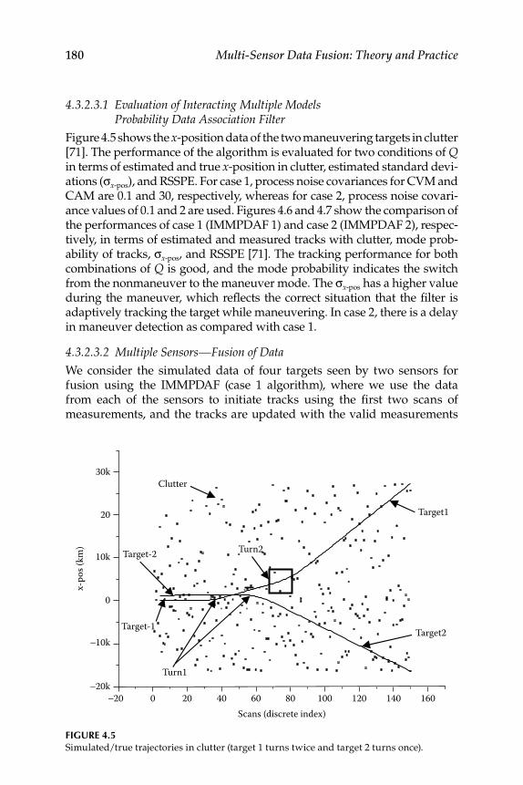
180 Multi-Sensor Data Fusion: Theory and Practice

4.3.2.3.1 Evaluation of Interacting Multiple Models Probability Data Association Filter

Figure 4.5 shows the x -position data of the two maneuvering targets in clutter [71]. The performance of the algorithm is evaluated for two conditions of Q in terms of estimated and true x -position in clutter, estimated standard devi-ations (σ x -pos ), and RSSPE. For case 1, process noise covariances for CVM and CAM are 0.1 and 30, respectively, whereas for case 2, process noise covari-ance values of 0.1 and 2 are used. Figures 4.6 and 4.7 show the comparison of the performances of case 1 (IMMPDAF 1) and case 2 (IMMPDAF 2), respec-tively, in terms of estimated and measured tracks with clutter, mode prob-ability of tracks, σ x -pos , and RSSPE [71]. The tracking performance for both combinations of Q is good, and the mode probability indicates the switch from the nonmaneuver to the maneuver mode. The σ x -pos has a higher value during the maneuver, which refl ects the correct situation that the fi lter is adaptively tracking the target while maneuvering. In case 2, there is a delay in maneuver detection as compared with case 1.

4.3.2.3.2 Multiple Sensors—Fusion of Data

We consider the simulated data of four targets seen by two sensors for fusion using the IMMPDAF (case 1 algorithm), where we use the data from each of the sensors to initiate tracks using the fi rst two scans of measurements, and the tracks are updated with the valid measurements

FIGURE 4.5 Simulated/true trajectories in clutter (target 1 turns twice and target 2 turns once).

Target-2

Target-1

−20 0 20 40 60 80 100 120 140 160−20k

−10k

0

10k

20

30kClutter

Target2

Target1

Turn2

Turn1

Scans (discrete index)

x-po

s (km

)

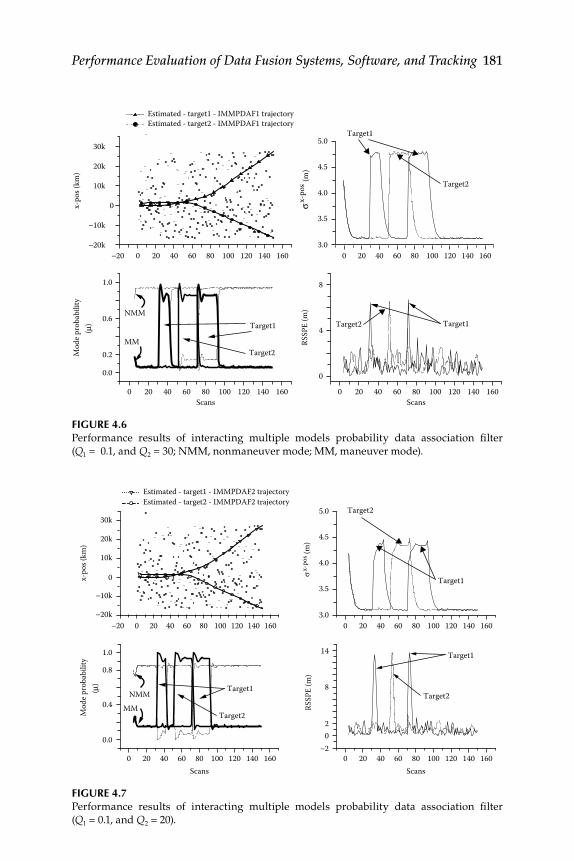
Performance Evaluation of Data Fusion Systems, Software, and Tracking 181

FIGURE 4.7 Performance results of interacting multiple models probability data association fi lter

( Q 1 = 0.1, and Q 2 = 20).

Mod

e pro

babi

lity

(μ)

0 20 40 60 80 100 120 140 160

0 20 40 60 80 100 120 140 1600 20 40 60 80 100Scans Scans

120 140 160

−20 0 20 40 60 80 100 120 140 160−20k

−10k

0

10k

20k

30k

Estimated - target1 - IMMPDAF2 trajectoryEstimated - target2 - IMMPDAF2 trajectory

x-po

s (km

)

3.0

3.5

4.0

4.5

5.0 Target2

Target1

sx-

pos (m

)

−202

8

14

Target2

Target1

RSSP

E (m

)

0.0

0.4

0.8

1.0

MMNMM

Target2

Target1

FIGURE 4.6 Performance results of interacting multiple models probability data association fi lter

( Q 1 = 0.1, and Q 2 = 30; NMM, nonmaneuver mode; MM, maneuver mode).

−20−20k

−10k

0

10k

20k

30k

Estimated - target1 - IMMPDAF1 trajectory Estimated - target2 - IMMPDAF1 trajectory

x-po

s (km

)

0.0

0.2

0.6

1.0

MM

NMM

Target2

Target1

Scans

Mod

e pro

babi

lity

(μ)

0 20 40 60 80 100 120 140 160

0 20 40 60 80 100 120 140 160

0 20 40 60 80 100 120 140 160

0

4

8

Target2

Scans

RSSP

E (m

)

Target1

Target2

Target1

0 20 40 60 80 100 120 140 1603.0

3.5

4.0

4.5

5.0

σx-

pos (m

)

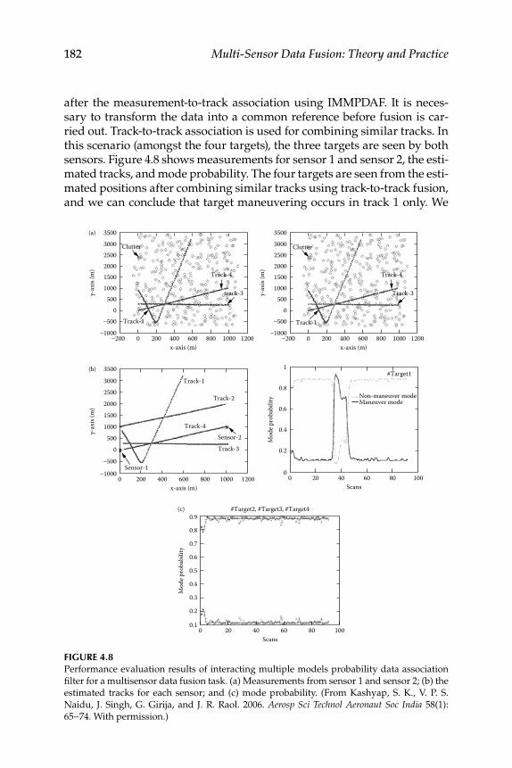
182 Multi-Sensor Data Fusion: Theory and Practice

after the measurement-to-track association using IMMPDAF. It is neces-sary to transform the data into a common reference before fusion is car-ried out. Track-to-track association is used for combining similar tracks. In this scenario (amongst the four targets), the three targets are seen by both sensors. Figure 4.8 shows measurements for sensor 1 and sensor 2, the esti-mated tracks, and mode probability. The four targets are seen from the esti-mated positions after combining similar tracks using track-to-track fusion, and we can conclude that target maneuvering occurs in track 1 only. We

FIGURE 4.8Performance evaluation results of interacting multiple models probability data association

fi lter for a multisensor data fusion task. (a) Measurements from sensor 1 and sensor 2; (b) the

estimated tracks for each sensor; and (c) mode probability. (From Kashyap, S. K., V. P. S.

Naidu, J. Singh, G. Girija, and J. R. Raol. 2006. Aerosp Sci Technol Aeronaut Soc India 58(1):

65−74. With permission.)

5001000

2000

y-ax

is (m

)

3000 Clutter

Track-1

track-3

Track-41500

2500

3500

0−500

−1000−200 0 200 400

x-axis (m)

(a)

(b)

(c)

600 800 1000 1200

5001000

2000

y-ax

is (m

)

3000

Sensor-1

Sensor-2Track-4

Track-2

#Target1

#Target2, #Target3, #Target4

Track-3

Track-1

1500

2500

3500

0−500

−10000 200 400

x-axis (m)600 800 1000 1200

0.4

Mod

e pro

babi

lity

0.6

0.8

1

0.2

00 20 40

Scans60

Non-maneuver modeManeuver mode

80 100

5001000

2000y-

axis

(m)

3000 Clutter

Track-1

Track-3

Track-41500

2500

3500

0−500

−1000−200 0 200 400

x-axis (m)600 800 1000 1200

0.4

Mod

e pro

babi

lity

0.6

0.8

0.9

0.2

0.10 20 40

Scans60 80 100

0.3

0.5

0.7

Performance Evaluation of Data Fusion Systems, Software, and Tracking 183

fi nd that the IMMPDAF gives realistic estimates during maneuvers and a lower RSSPE during the nonmaneuvering phase of the targets.

4.4 Evaluation of Converted Measurement and

Modified Extended Kalman Filters

Many algorithms are available for obtaining improved accuracy with radar measurements in target tracking applications using KF [72,73]; however, it would be desirable to use a scheme with lower computational complex-ity when the data rate is high and the available computing power is lim-ited. Target dynamics are better described in Cartesian coordinates, since the dynamics are uncoupled and linear, whereas radars measure the target range, elevation, and azimuth, yielding nonlinear relations between the states and measurements. The inaccuracies of the measurements will have a direct effect on the performance of the tracking algorithms. For target track-ing using the radar measurements, two approaches are commonly used:

1. Linear KF or converted measurements KF (CMKF): In this method, the measurements used for updating the states are generated by converting the raw measurements in polar frame to the Cartesian frame, rendering the measurements as the linear functions of the states. The converted measurement errors would become corre-lated. The cross-range measurement errors would be large, the mean of the errors would be high, and a debiasing process would be required. Thus, the measurement noise covariance matrix should include cross-covariance terms to account for correlated measurement errors. Analytical expressions for the debiased CMKF (CMKF-D) are available in [72]. This would necessitate evaluation of complex equations.

2. EKF approach: In this method, the measurements used for updat-ing the states are the range, azimuth, and elevation in polar frame. The measurements are nonlinear functions of the states yielding a mixed coordinates fi lter. In the EKF, the initial covariance depends on the initial converted measurements and the gains depend on the accuracy of the subsequent linearization. A simple way to handle the nonlinearities [74] is to process the radar measurements sequentially in the order of elevation, azimuth, and range, while linearizing the nonlinear equations with respect to the estimated states. This results in considerable computational savings. When the nonlinearities are strong, modifi ed expressions for the mean and covariance errors can be used and a modifi ed EKF (MEKF; measurements are still sequentially processed) was proposed [73].

184 Multi-Sensor Data Fusion: Theory and Practice

To achieve better accuracy, both methods require certain modifi cations in order to handle the bias and measurement error covariance in the conventional linear KF and EKF. In this section, an alternative method of achieving debiasing and obtaining an estimate of the measurement error covariance using converted radar measurements is proposed [75,76]. The method based on error model converted measurement KF (ECMKF) presupposes the availability of very accurate reference data from an independent measurement source. The GPS or differential GPS (DGPS) method gives very accurate measurements of position, and hence, these data can be used to get accurate estimates of the bias and measurement noise covariance of the converted measurements in the Cartesian frame using KF with error state-space formulation [77]. Here, the estimated bias is used for correction in the converted measurements and the estimated covariance values used in the ECMKF. The performance of the ECMKF is compared with the error model MEKF (EMEKF) algorithm, and the latter handles the measurements of range, azimuth, and elevation directly. The simulated data of a target with different measurement accuracies are used. The algorithms are implemented in PC MATLAB and evaluated in terms of RSSPE and PFE with respect to true data. These algorithms are also used for tracking a moving target from ground-based radar measurements when GPS measurements of position of the aircraft are available. For the sake of comparison, the results of CMKF-D [72] are also presented.

4.4.1 Error Model Converted Measurement Kalman Filter and Error Model Modified Extended Kalman Filter Algorithms

The target-tracking model is described in Cartesian coordinate system with additive noise:

Xk+1

= FXk + Gwk (4.41)

Here, the vector X consists of the position and velocity of the target

(X = [x y z &x &y &z ]), the process noise w is assumed to be white, and the zero mean with covariance matrix Q . The ground-based radar provides measurements of range (rm), azimuth (qm) and elevation (fm). The measure-ment model is given as:

rm

θm

φm

⎡

⎣

⎢⎢⎢

⎤

⎦

⎥⎥⎥

= h(Χk ) + vk =

x2 + y2 + z2

tan−1 y

x⎛⎝⎜

⎞⎠⎟

tan −1 z

x2 + y2

⎡

⎣

⎢⎢⎢⎢⎢⎢⎢⎢⎢

⎤

⎦

⎥⎥⎥⎥⎥⎥⎥⎥⎥

+vr

vθ

vφ

⎡

⎣

⎢⎢⎢

⎤

⎦

⎥⎥⎥

(4.42)

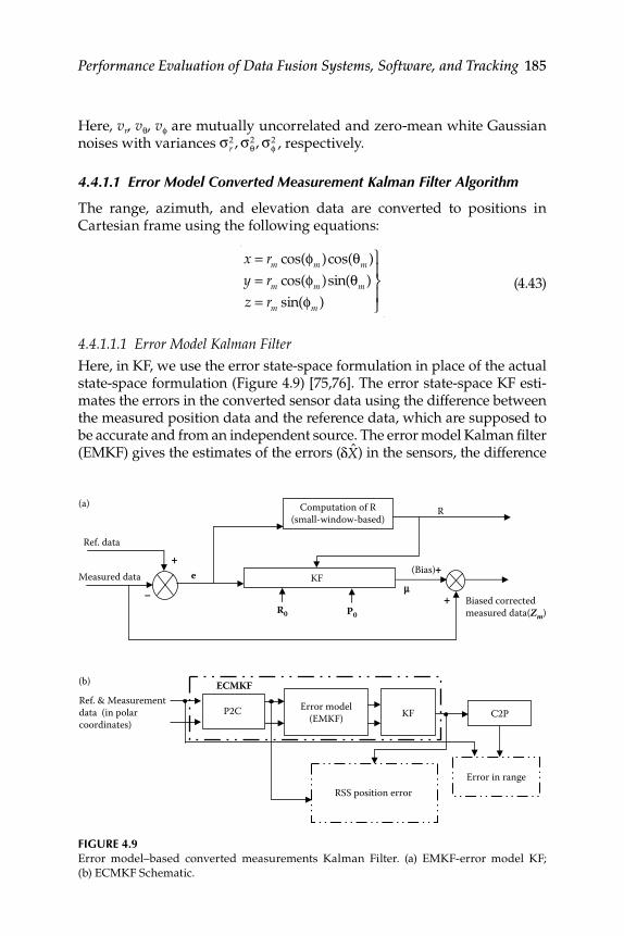
Performance Evaluation of Data Fusion Systems, Software, and Tracking 185

Here, vr, vθ, vφ are mutually uncorrelated and zero-mean white Gaussian noises with variances σr

2, σθ2, σφ

2 , respectively.

4.4.1.1 Error Model Converted Measurement Kalman Filter Algorithm

The range, azimuth, and elevation data are converted to positions in Cartesian frame using the following equations:

x = rm cos(φm )cos(θm )

y = rm cos(φm )sin(θm )

z = rm sin(φm )

⎫

⎬⎪

⎭⎪

(4.43)

4.4.1.1.1 Error Model Kalman Filter

Here, in KF, we use the error state-space formulation in place of the actual state-space formulation (Figure 4.9) [75,76]. The error state-space KF esti-mates the errors in the converted sensor data using the difference between the measured position data and the reference data, which are supposed to be accurate and from an independent source. The error model Kalman fi lter (EMKF) gives the estimates of the errors (δX) in the sensors, the difference

FIGURE 4.9 Error model–based converted measurements Kalman Filter. (a) EMKF-error model KF;

(b) ECMKF Schematic.

(a)

(b)

Ref. & Measurementdata (in polarcoordinates)

Error in range

P2C Error model(EMKF) KF C2P

RSS position error

ECMKF

KF −

+

+µ

Biased correctedmeasured data(Zm)

R

R0 P0

Computation of R(small-window-based)

e (Bias)+

Ref. data

Measured data

186 Multi-Sensor Data Fusion: Theory and Practice

between the converted radar data and the GPS/DGPS reference data, and the noise statistics. These error estimates can be used for the correction of actual measurements. The error state model is given as

δXk+1

= F δXk + Gwk (4.44)

δZk = HδXk + vk (4.45)

Here, δX is the vector of position and velocity errors in all the three axes and δZ is a vector of computed position error in all the three axes (GPS− radar measurement). This estimated position error is used to correct the converted data that are used for measurement update in the KF. The ECMKF algorithm follows the conventional linear KF equations:

Initialization:

X0 0= X

0, P

0 0= PX0

(4.46)

Time propagation:

%Xk k−1= Fk−1

Xk−1 k−1

%Pk k−1= Fk−1

Pk−1 k−1Fk−1

+ Gk−1Qk−1

Gk−1T

(4.47)

State update by measurements:

S = H %Pk|k−1HT + R

K = %Pk|k−1HT (S)−1

Xk|k = %Xk|k−1+ K(Zm − H %Xk|k−1

)

Pk|k = %Pk|k−1− KSKT

(4.48)

The scheme for ECMKF is given in Figure 4.9 [76].

4.4.1.2 Error Model Modifi ed Extended Kalman Filter Algorithm

In this scheme, the radar measurements are processed one component at a time in a preferred order: elevation, azimuth, and range. The initialization and time propagation are done using Equations 4.46 and 4.47. The error model states are r , θ, and φ. The measurement update with respect to the range measurement includes extra terms in the measurement covariance part to account for nonlinear cross-coupling among the range, azimuth, and elevation measurements. Figure 4.10 shows the scheme of EMEKF [75,76]. It is assumed that the measurements are processed starting with φ and predicted states and then θ and range [73,76].

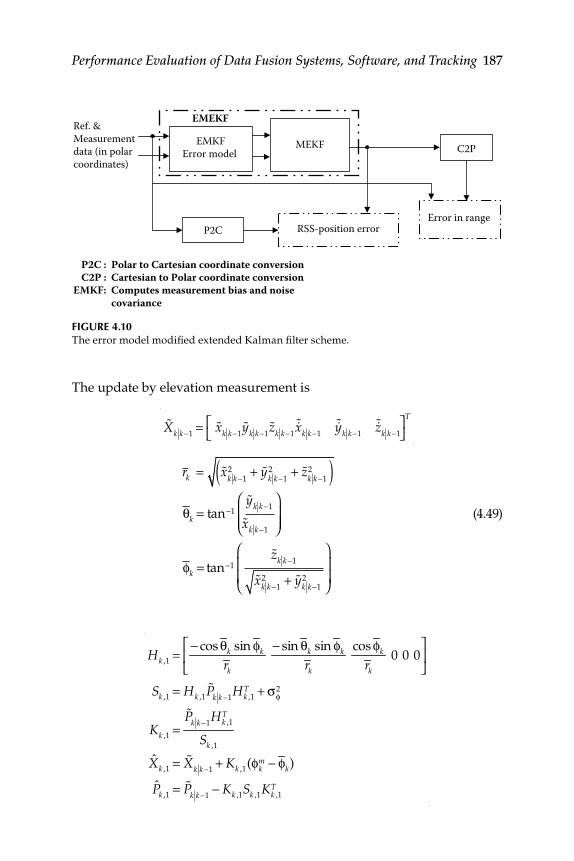
Performance Evaluation of Data Fusion Systems, Software, and Tracking 187

The update by elevation measurement is

%Xk k−1

= %xk k−1%yk k−1

%zk k−1&%xk k−1

&%yk k−1&%zk k−1

⎡⎣

⎤⎦

T

rk = %xk k−12 + %y

k k−12 + %z

k k−12( )

θk = tan−1%yk k−1

%xk k−1

⎛

⎝⎜⎜

⎞

⎠⎟⎟

φk = tan−1%zk k−1

%xk k−12 + %yk k−1

2

⎛

⎝

⎜⎜

⎞

⎠

⎟⎟

(4.49)

Hk ,1=

− cos θk sin φk

rk

− sin θk sin φk

rk

cos φk

rk

0 0 0⎡

⎣⎢

⎤

⎦⎥

Sk ,1= Hk ,1

%Pk k−1Hk ,1

T + σφ2

Kk ,1=

%Pk k−1Hk ,1

T

Sk ,1

Xk ,1= %Xk k−1

+ Kk ,1(φk

m − φk)

Pk ,1= %Pk k−1

− Kk ,1Sk ,1

Kk ,1T

FIGURE 4.10 The error model modifi ed extended Kalman fi lter scheme.

EMEKF

Error in range

P2C : Polar to Cartesian coordinate conversion C2P : Cartesian to Polar coordinate conversionEMKF: Computes measurement bias and noise covariance

EMKFError model

P2C

MEKF

RSS-position error

C2P

Ref. &Measurementdata (in polarcoordinates)

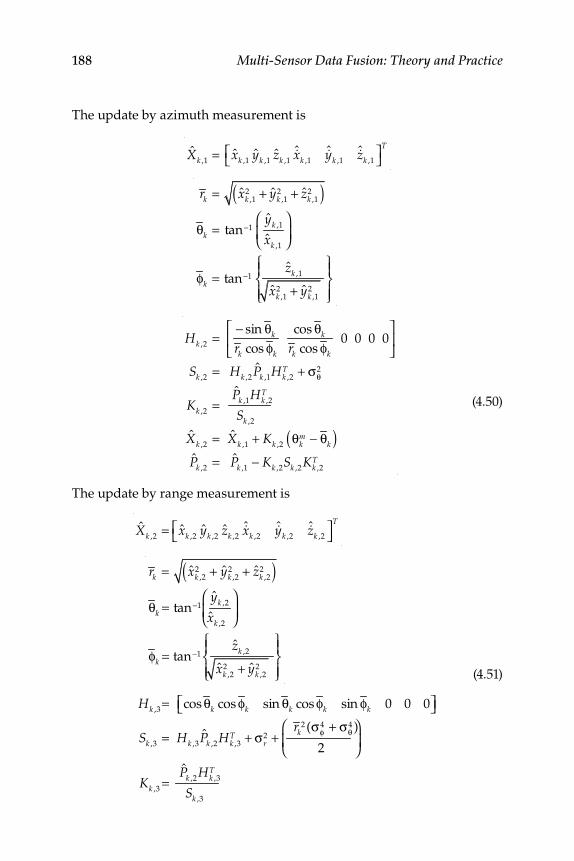
188 Multi-Sensor Data Fusion: Theory and Practice

The update by azimuth measurement is

Xk ,1

= xk ,1yk ,1

zk ,1&xk ,1

&yk ,1&zk ,1

⎡⎣ ⎤⎦T

rk = xk ,12 + yk ,1

2 + zk ,12( )

θk = tan−1yk ,1

xk ,1

⎛

⎝⎜⎞

⎠⎟

φk = tan−1zk ,1

xk ,12 + yk ,1

2

⎧⎨⎪

⎩⎪

⎫⎬⎪

⎭⎪

Hk ,2=

− sin θk

rk cos φk

cos θk

rk cos φk

0 0 0 0⎡

⎣⎢

⎤

⎦⎥

Sk ,2= Hk ,2

Pk ,1Hk ,2

T + σθ2

Kk ,2=

Pk ,1Hk ,2

T

Sk ,2

Xk ,2= Xk ,1

+ Kk ,2θk

m − θk( )Pk ,2

= Pk ,1− Kk ,2

Sk ,2Kk ,2

T

(4.50)

The update by range measurement is

Xk ,2

= xk ,2yk ,2

zk ,2&xk ,2

&yk ,2&zk ,2

⎡⎣ ⎤⎦T

rk = xk ,22 + yk ,2

2 + zk ,22( )

θk = tan−1yk ,2

xk ,2

⎛

⎝⎜⎞

⎠⎟

φk = tan−1zk ,2

xk ,22 + yk ,2

2

⎧⎨⎪

⎩⎪

⎫⎬⎪

⎭⎪ (4.51)

Hk ,3= cos θk cos φk sin θk cos φk sin φk 0 0 0⎡⎣ ⎤⎦

Sk ,3= Hk ,3

Pk ,2Hk ,3

T + σr2 +

rk2 (σφ

4 + σθ4 )

2

⎛

⎝⎜

⎞

⎠⎟

Kk ,3=

Pk ,2Hk ,3

T

Sk ,3

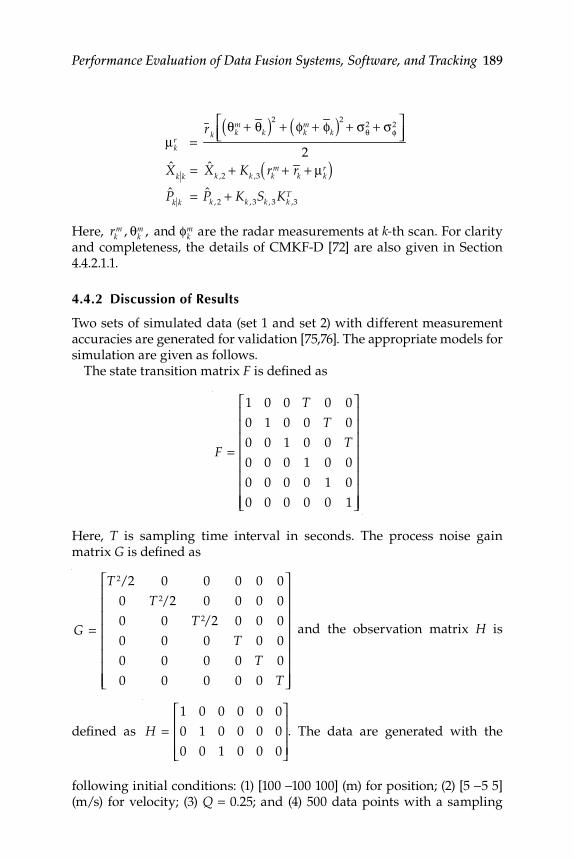
Performance Evaluation of Data Fusion Systems, Software, and Tracking 189

μkr =

rkθk

m + θk( )2+ φk

m + φk( )2+ σθ

2 + σφ2⎡

⎣⎢⎤⎦⎥

2

Xk k = Xk ,2+ Kk ,3

rkm + rk + μk

r( )Pk k = Pk , 2

+ Kk , 3Sk , 3

Kk ,3T

Here, rkm , θk

m , and φkm are the radar measurements at k- th scan. For clarity

and completeness, the details of CMKF-D [72] are also given in Section 4.4.2.1.1.

4.4.2 Discussion of Results

Two sets of simulated data (set 1 and set 2) with different measurement accuracies are generated for validation [75,76]. The appropriate models for simulation are given as follows.

The state transition matrix F is defi ned as

F =

1 0 0 T 0 0

0 1 0 0 T 0

0 0 1 0 0 T

0 0 0 1 0 0

0 0 0 0 1 0

0 0 0 0 0 1

⎡

⎣

⎢⎢⎢⎢⎢⎢⎢⎢

⎤

⎦

⎥⎥⎥⎥⎥⎥⎥⎥

Here, T is sampling time interval in seconds. The process noise gain matrix G is defi ned as

G =

T 2/2 0 0 0 0 0

0 T 2/2 0 0 0 0

0 0 T 2/2 0 0 0

0 0 0 T 0 0

0 0 0 0 T 0

0 0 0 0 0 T

⎡

⎣

⎢⎢⎢⎢⎢⎢⎢⎢

⎤

⎦

⎥⎥⎥⎥⎥⎥⎥⎥

and the observation matrix H is

defi ned as

H =1 0 0 0 0 0

0 1 0 0 0 0

0 0 1 0 0 0

⎡

⎣

⎢⎢⎢

⎤

⎦

⎥⎥⎥. The data are generated with the

following initial conditions: (1) [100 −100 100] (m) for position; (2) [5 −5 5] (m/s) for velocity; (3) Q = 0.25; and (4) 500 data points with a sampling

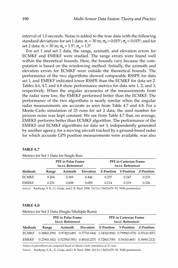
190 Multi-Sensor Data Fusion: Theory and Practice

interval of 1.0 seconds. Noise is added to the true data with the following standard deviations for set 1 data: σr = 30 m; σθ = 0.015°; σφ = 0.015°; and for set 2 data: σr = 30 m; σθ = 1.5°; σϕ = 1.5° .

For set 1 and set 2 data, the range, azimuth, and elevation errors for ECMKF and EMEKF were studied. The range errors were found well within the theoretical bounds. Here, the bounds vary because the com-putation is based on the windowing method. Initially, the azimuth and elevation errors for ECMKF were outside the theoretical bounds. The performance of the two algorithms showed comparable RSSPE for data set 1, and EMEKF indicated lower RSSPE than the ECMKF for data set 2. Tables 4.6, 4.7, and 4.8 show performance metrics for data sets 1, 2, and 3, respectively. When the angular accuracies of the measurements from the radar were low, the EMEKF performed better than the ECMKF. The performance of the two algorithms is nearly similar when the angular radar measurements are accurate as seen from Table 4.7 and 4.8. For a Monte-Carlo simulation of 25 runs for set 2 data, the seed number for process noise was kept constant. We see from Table 4.7 that, on average, EMEKF performs better than ECMKF algorithm. The performance of the EMEKF and ECMKF algorithms for data set 3, independently generated by another agency, for a moving aircraft tracked by a ground-based radar for which accurate GPS position measurements were available, was also

TABLE 4.7

Metrics for Set 1 Data for Single Run

Methods

PFE in Polar Frame

(w.r.t. Reference)

PFE in Cartesian Frame

(w.r.t. Reference)

Range Azimuth Elevation X-Position Y-Position Z-Position

ECMKF 0.204 0.369 0.446 0.237 0.247 0.233

EMEKF 0.221 0.008 0.009 0.214 0.219 0.226

Source: Kashyap, S. K., G. Girija, and J. R. Raol. 2006. Def Sci J 56(5):679−92. With permission.

TABLE 4.8

Metrics for Set 2 Data (Single/Multiple Runs)

Methods

PFE in Polar Frame

(w.r.t. Reference)

PFE in Cartesian Frame

(w.r.t. Reference)

Range Azimuth Elevation X-Position Y-Position Z-Position

ECMKF 0.388(0.299) 0.974(0.649) 0.777(0.544) 1.343(0.894) 0.7998(0.575) 0.551(0.307)

EMEKF 0.239(0.182) 0.5235(0.581) 0.481(0.237) 0.728(0.749) 0.563(0.465) 0.369(0.212)

Values in parentheses are computed based on Monte-Carlo simulation of 25 runs.Source: Kashyap, S. K., G. Girija, and J. R. Raol. 2006. Def Sci J 56(5):679−92. With permission.

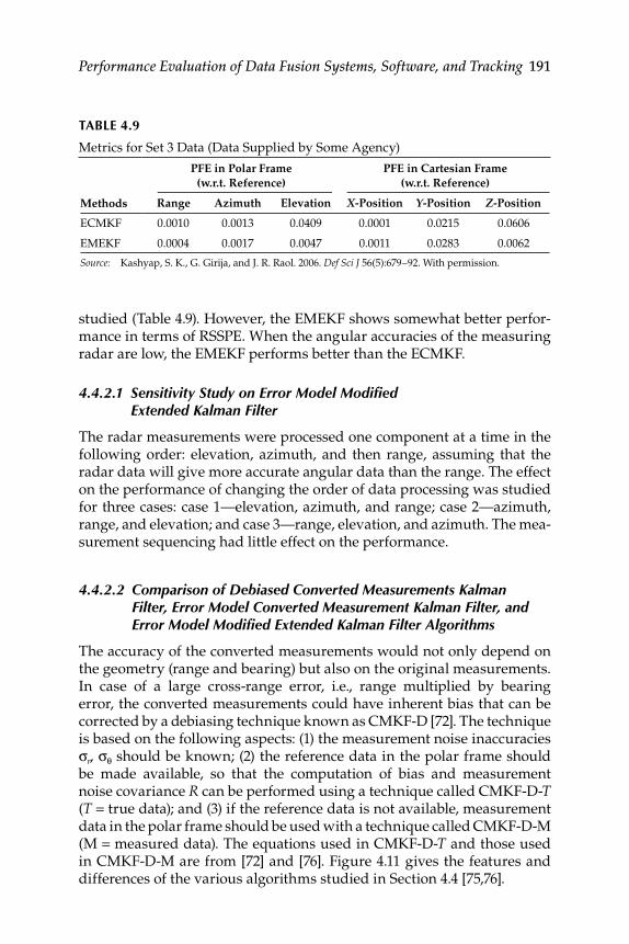
Performance Evaluation of Data Fusion Systems, Software, and Tracking 191

studied (Table 4.9). However, the EMEKF shows somewhat better perfor-mance in terms of RSSPE. When the angular accuracies of the measuring radar are low, the EMEKF performs better than the ECMKF.

4.4.2.1 Sensitivity Study on Error Model Modifi ed Extended Kalman Filter

The radar measurements were processed one component at a time in the following order: elevation, azimuth, and then range, assuming that the radar data will give more accurate angular data than the range. The effect on the performance of changing the order of data processing was studied for three cases: case 1—elevation, azimuth, and range; case 2—azimuth, range, and elevation; and case 3—range, elevation, and azimuth. The mea-surement sequencing had little effect on the performance.

4.4.2.2 Comparison of Debiased Converted Measurements Kalman Filter, Error Model Converted Measurement Kalman Filter, and Error Model Modifi ed Extended Kalman Filter Algorithms

The accuracy of the converted measurements would not only depend on the geometry (range and bearing) but also on the original measurements. In case of a large cross-range error, i.e., range multiplied by bearing error, the converted measurements could have inherent bias that can be corrected by a debiasing technique known as CMKF-D [72]. The technique is based on the following aspects: (1) the measurement noise inaccuracies σr, σθ should be known; (2) the reference data in the polar frame should be made available, so that the computation of bias and measurement noise covariance R can be performed using a technique called CMKF-D- T ( T = true data); and (3) if the reference data is not available, measurement data in the polar frame should be used with a technique called CMKF-D-M (M = measured data). The equations used in CMKF-D- T and those used in CMKF-D-M are from [72] and [76]. Figure 4.11 gives the features and differences of the various algorithms studied in Section 4.4 [75,76].

TABLE 4.9

Metrics for Set 3 Data (Data Supplied by Some Agency)

Methods

PFE in Polar Frame

(w.r.t. Reference)

PFE in Cartesian Frame

(w.r.t. Reference)

Range Azimuth Elevation X-Position Y-Position Z-Position

ECMKF 0.0010 0.0013 0.0409 0.0001 0.0215 0.0606

EMEKF 0.0004 0.0017 0.0047 0.0011 0.0283 0.0062

Source: Kashyap, S. K., G. Girija, and J. R. Raol. 2006. Def Sci J 56(5):679−92. With permission.

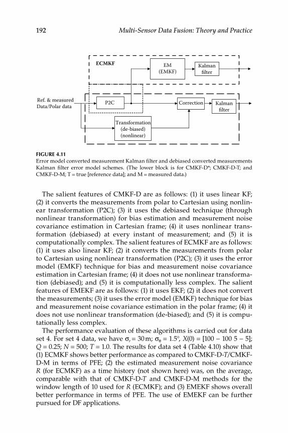
192 Multi-Sensor Data Fusion: Theory and Practice

The salient features of CMKF-D are as follows: (1) it uses linear KF; (2) it converts the measurements from polar to Cartesian using nonlin-ear transformation (P2C); (3) it uses the debiased technique (through nonlinear transformation) for bias estimation and measurement noise covariance estimation in Cartesian frame; (4) it uses nonlinear trans-formation (debiased) at every instant of measurement; and (5) it is computationally complex. The salient features of ECMKF are as follows: (1) it uses also linear KF; (2) it converts the measurements from polar to Cartesian using nonlinear transformation (P2C); (3) it uses the error model (EMKF) technique for bias and measurement noise covariance estimation in Cartesian frame; (4) it does not use nonlinear transforma-tion (debiased); and (5) it is computationally less complex. The salient features of EMEKF are as follows: (1) it uses EKF; (2) it does not convert the measurements; (3) it uses the error model (EMKF) technique for bias and measurement noise covariance estimation in the polar frame; (4) it does not use nonlinear transformation (de-biased); and (5) it is compu-tationally less complex.

The performance evaluation of these algorithms is carried out for data set 4. For set 4 data, we have σr = 30 m; σθ = 1.5°, X (0) = [100 − 100 5 − 5]; Q = 0.25; N = 500; T = 1.0. The results for data set 4 (Table 4.10) show that (1) ECMKF shows better performance as compared to CMKF-D- T /CMKF-D-M in terms of PFE; (2) the estimated measurement noise covariance R (for ECMKF) as a time history (not shown here) was, on the average, comparable with that of CMKF-D- T and CMKF-D-M methods for the window length of 10 used for R (ECMKF); and (3) EMEKF shows overall better performance in terms of PFE. The use of EMEKF can be further pursued for DF applications.

FIGURE 4.11 Error model converted measurement Kalman fi lter and debiased converted measurements

Kalman fi lter error model schemes. (The lower block is for CMKF-D*; CMKF-D-T; and

CMKF-D-M; T = true [reference data]; and M = measured data.)

Ref. & measuredData/Polar data P2C

EM(EMKF)

Kalmanfilter

Kalmanfilter

Transformation(de-biased)(nonlinear)

Correction

ECMKF

Performance Evaluation of Data Fusion Systems, Software, and Tracking 193

4.5 Estimation of Attitude Using Low-Cost Inertial

Platforms and Kalman Filter Fusion

Inertial measurement units (IMUs), when combined with GPS, can pro-vide critical information needed for navigation [78]. An IMU system consists of a set of spinning-mass vertical gyros that provide analog outputs and is usually heavy and expensive to maintain. Because of its analog nature, the IMU requires data conversion when interfaced to a digital navigation system. This increases the overall cost and complexity. High-performance inertial-grade IMUs of avionics systems show superior performance specifi cations. However, because of the high costs, their use is not preferred in many applications. A suitable combination of low-cost microelectrical mechanical sensors (MEMS) and digital signal processing techniques can provide an inexpensive and adaptable alternative to exist-ing IMUs. The closely coupled integration of the sensors, data acquisition systems, and KF-based fusion algorithms allow the MEMS-based IMU to provide an accurate estimation of the attitude of a fl ight vehicle with a performance comparable to some of the older IMUs.

Two small and extensively instrumented vehicles, ALEX-I and ALEX-II, were developed by and fl ight-tested at the Institute of Flight Systems and Research, at the German Aerospace Center in Germany, to identify the dynamic behavior of a parafoil-load system (Figure 4.12) [78−81]. The system is also suited for the investigation of guidance, navigation, and control (GNC) concepts for the autonomous landing. A small sensor plat-form, called a miniaturized inertial platform (MIP), was utilized, consist-ing of small, low-cost accelerometers, rate gyros, magnetometers, and a temperature transducer. Deriving the position data as the data from the GPS receiver that were available from this small sensor box was very criti-cal. The attitudes must be computed from the output of the three angular

TABLE 4.10

Metrics for CMKF-D, ECMKF, and EMEKF (Set 4 Data for Single Run)

Methods

PFE in Polar Frame

(w.r.t. Reference)

PFE in Cartesian Frame

(w.r.t. Reference)

Range Azimuth X-Position Y-Position

CMKF-D-T 0.5205 1.4889 0.8432 1.2734

CMKF-D-M 0.5267 1.4960 0.8404 1.2764

ECMKF 0.4867 1.2271 0.7741 1.1584

EMEKF 0.4781 0.6715 0.4062

Source: Kashyap, S. K., G. Girija, and J. R. Raol. 2006. Def Sci J 56(5):679−92. With permission.

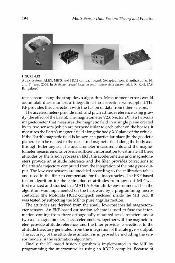
194 Multi-Sensor Data Fusion: Theory and Practice

rate sensors using the strap down algorithm. Measurement errors would accumulate due to numerical integration if no corrections were applied. The KF provides this correction with the fusion of data from other sensors.

The accelerometers provide a roll and pitch attitude reference using grav-ity (the effect of the Earth). The magnetometer V2 X (vector 2X) is a two-axis magnetometer that measures the magnetic fi eld in a single plane created by its two sensors (which are perpendicular to each other on the board). It measures the Earth’s magnetic fi eld along the body X - Y plane of the vehicle. If the Earth’s magnetic fi eld is known at a particular place (in the geodetic plane), it can be related to the measured magnetic fi eld along the body axis through Euler angles. The accelerometer measurements and the magne-tometer measurements provide suffi cient information to estimate all three attitudes by the fusion process in EKF: the accelerometers and magnetom-eters provide an attitude reference and the fi lter provides corrections to the attitude trajectory computed from the integration of the rate gyros out-put. The low-cost sensors are modeled according to the calibration tables and used in the fi lter to compensate for the inaccuracies. The EKF-based fusion algorithm for the estimation of attitudes from low-cost MIP was fi rst realized and studied in a MATLAB/Simulink® environment. Then the algorithm was implemented on the hardware by a programming micro-controller (the Motorola HC12 compact) enclosed inside the MIP box. It was tested by subjecting the MIP to pure angular motion.

The attitudes are derived from the small, low-cost inertial magnetom-eter sensors. An EKF-based estimation scheme is used to fuse the infor-mation coming from three orthogonally mounted accelerometers and a two-axis magnetometer. The accelerometers, together with the magnetom-eter, provide attitude reference, and the fi lter provides corrections to the attitude trajectory generated from the integration of the rate gyros output. The accuracy of the attitude estimation is improved by including the sen-sor models in the estimation algorithm.

Finally, the KF-based fusion algorithm is implemented in the MIP by programming the microcontroller using an ICC12 compiler. Because of

FIGURE 4.12 ALEX system: ALEX, MIPS, and HC12 compact board. (Adapted from Shanthakumar, N.,

and T. Jann. 2004. In Sadhana, special issue on multi-sensor data fusion, ed. J. R. Raol, IAS,

Bangalore.)

Performance Evaluation of Data Fusion Systems, Software, and Tracking 195

the computational speed limitations of the microcontroller, no augmented states (sensor bias states) are included in the model. The decision to imple-ment this minimal set of states (only four quaternion states) model is arrived at based on the assumption that the sensor model used in the fi lter model is almost accurate and the output is bias free. This four-state model is thor-oughly validated in the MATLAB/Simulink setup before implementing on microcontroller. The algorithm is tested and evaluated by subjecting the MIP to pure angular motion and holding it at different orientations.

4.5.1 Hardware System

The MIP is a miniaturized multisensor inertial platform (shown in Figure 4.12 [78]) with two motherboards stacked one above the other; the sensor board consists of all the sensors, and the other board consists of a micro-controller HC12 compact, which is used to acquire and process the sensors’ output data. The sensor board consists of (1) three orthogonally mounted rate gyroscopes, (2) three orthogonally mounted linear accelerometers, (3) a temperature transducer, and (4) a two-axis magnetometer with two sen-sors along the body X - Y axis. The temperature transducer records the tem-perature variation effect on the other sensors. These sensors are of a low cost and small size (MEMS class from aerospace consumer bulk market). A GPS receiver connected to the MIP via one of the serial communication interfaces (SCI) can provide the position information. The data processing unit of MIP is the HC12 compact with a 16 Mhz clock speed, and is an uni-versal microcontroller module on the basis of a Motorola MC68HC812A4 microcontroller unit (MCU) [82]. The HC12 compact has the follow-ing peripheral units: (1) 512 kB fl ash memory and 256 kB random access memory (RAM), (2) 12 bit, 11 channels analog-to-digital conversion (ADC), (3) 12 bit, 2 channels digital-to-analog conversion (DAC), (4) controller area network (CAN), (5) RS232 interface driver, (6) beeper, and (7) light- emitting diode (LED) indicator. The outputs of rate gyros, accelerometers, and temperature transducer are analog and are connected to the ADC of the microcontroller board. The output of magnetometer is digital and is connected directly to the microcontroller (fi gure 2d in [78]).

4.5.2 Sensor Modeling

Low-cost sensors suffer from inaccuracy and are greatly infl uenced by temperature variation. Such inaccuracies and subjectivity to temperature variations are modeled and compensated for in order to get quality measurements. Based on the calibration data, the sensors’ misalignment, temperature drift, and center of gravity (CG) offsets are modeled (see Part 5.2). These models represent the true sensor model and are included as Simulink blocks for generating the sensor output; the inverse model is used in the fi lter for estimating the attitudes [78].

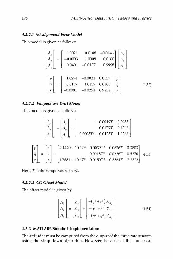
196 Multi-Sensor Data Fusion: Theory and Practice

4.5.2.1 Misalignment Error Model

This model is given as follows:

Ax

Ay

Az

⎡

⎣

⎢⎢⎢

⎤

⎦

⎥⎥⎥

m

=

1.0021 0.0188 −0.0146

− 0.0093 1.0008 0.0160

0.0401 −0.0137 0.9998

⎡

⎣

⎢⎢⎢

⎤

⎦

⎥⎥⎥

Ax

Ay

Az

⎡

⎣

⎢⎢⎢

⎤

⎦

⎥⎥⎥

t

p

q

r

⎡

⎣

⎢⎢⎢

⎤

⎦

⎥⎥⎥

m

=

1.0294 −0.0024 0.0157

0.0139 1.0137 0.0100

−0.0091 −0.0254 0.9838

⎡

⎣

⎢⎢⎢

⎤

⎦

⎥⎥⎥

p

q

r

⎡

⎣

⎢⎢⎢

⎤

⎦

⎥⎥⎥

t

(4.52)

4.5.2.2 Temperature Drift Model

This model is given as follows:

Ax

Ay

Az

⎡

⎣

⎢⎢⎢

⎤

⎦

⎥⎥⎥

m

=Ax

Ay

Az

⎡

⎣

⎢⎢⎢

⎤

⎦

⎥⎥⎥

t

+ − 0.0049T + 0.2955

− 0.0179T + 0.4348

−0.0005T 2 + 0.0425T − 1.0268

⎡

⎣

⎢⎢⎢

⎤

⎦

⎥⎥⎥

p

q

r

⎡

⎣

⎢⎢⎢

⎤

⎦

⎥⎥⎥

m

=p

q

r

⎡

⎣

⎢⎢⎢

⎤

⎦

⎥⎥⎥

t

+

4.1420 × 10−5T 3 − 0.0039T 2 + 0.0876T − 0.3803

0.0018T 2 − 0.0236T − 0.5370

1.7881 × 10−4T 3 − 0.0150T 2 + 0.3564T − 2.2526

⎡

⎣

⎢⎢⎢

⎤

⎦

⎥⎥⎥

(4.53)

Here, T is the temperature in °C.

4.5.2.3 CG Offset Model

The offset model is given by:

Ax

Ay

Az

⎡

⎣

⎢⎢⎢

⎤

⎦

⎥⎥⎥

m

≅Ax

Ay

Az

⎡

⎣

⎢⎢⎢

⎤

⎦

⎥⎥⎥

t

+

− q2 + r2( ) XAx

− p2 + r2( ) YAy

− p2 + q2( ) ZAz

⎡

⎣

⎢⎢⎢⎢

⎤

⎦

⎥⎥⎥⎥

(4.54)

4.5.3 MATLAB®/Simulink Implementation

The attitudes must be computed from the output of the three rate sensors using the strap-down algorithm. However, because of the numerical

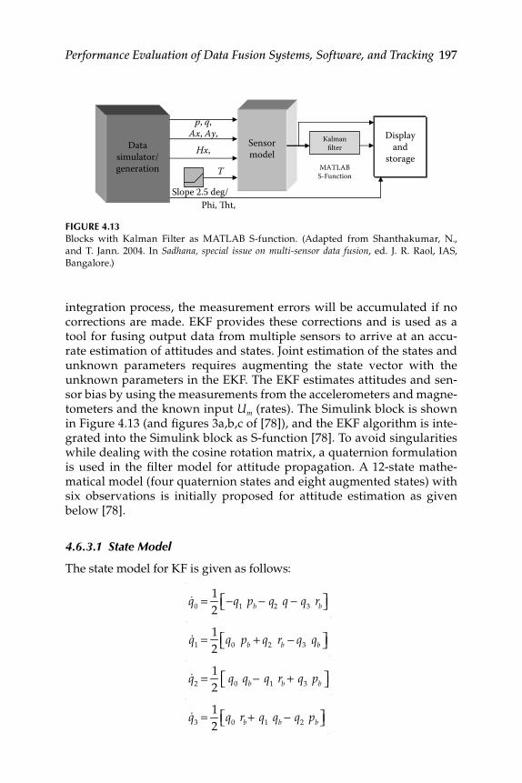
Performance Evaluation of Data Fusion Systems, Software, and Tracking 197

integration process, the measurement errors will be accumulated if no corrections are made. EKF provides these corrections and is used as a tool for fusing output data from multiple sensors to arrive at an accu-rate estimation of attitudes and states. Joint estimation of the states and unknown parameters requires augmenting the state vector with the unknown parameters in the EKF. The EKF estimates attitudes and sen-sor bias by using the measurements from the accelerometers and magne-tometers and the known input Um (rates). The Simulink block is shown in Figure 4.13 (and fi gures 3a,b,c of [78]), and the EKF algorithm is inte-grated into the Simulink block as S-function [78]. To avoid singularities while dealing with the cosine rotation matrix, a quaternion formulation is used in the fi lter model for attitude propagation. A 12-state mathe-matical model (four quaternion states and eight augmented states) with six observations is initially proposed for attitude estimation as given below [78].

4.6.3.1 State Model

The state model for KF is given as follows:

&q

0= 1

2−q

1 pb − q

2 q − q

3 rb⎡⎣ ⎤⎦

&q

1= 1

2q

0 pb + q

2 rb − q

3 qb⎡⎣ ⎤⎦

&q

2= 1

2 q

0 qb − q

1 rb + q

3 pb⎡⎣ ⎤⎦

&q

3= 1

2q

0 rb+ q

1 qb − q

2 pb⎡⎣ ⎤⎦

FIGURE 4.13 Blocks with Kalman Filter as MATLAB S-function. (Adapted from Shanthakumar, N.,

and T. Jann. 2004. In Sadhana, special issue on multi-sensor data fusion, ed. J. R. Raol, IAS,

Bangalore.)

Datasimulator/generation

Sensormodel

Kalmanfilter

Displayand

storage

p, q,Ax, Ay,

T

Hx,

Phi, Tht,

MATLABS-Function

Slope 2.5 deg/

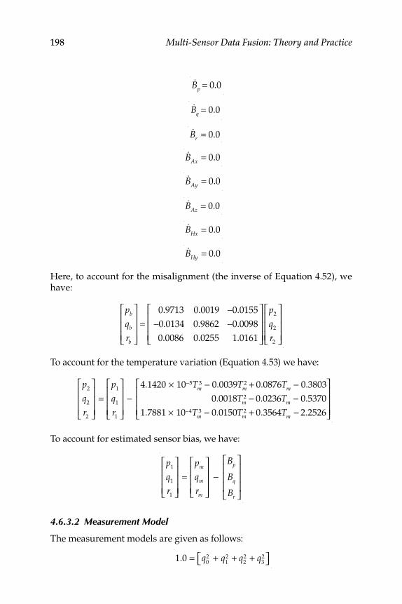
198 Multi-Sensor Data Fusion: Theory and Practice

&Bp = 0.0

&Bq = 0.0

&Br = 0.0

&BAx = 0.0

&BAy = 0.0

&BAz = 0.0

&BHx = 0.0

&BHy = 0.0

Here, to account for the misalignment (the inverse of Equation 4.52), we have:

pb

qb

rb

⎡

⎣

⎢⎢⎢

⎤

⎦

⎥⎥⎥

= 0.9713 0.0019 −0.0155

−0.0134 0.9862 −0.0098

0.0086 0.0255 1.0161

⎡

⎣

⎢⎢⎢

⎤

⎦

⎥⎥⎥

p2

q2

r2

⎡

⎣

⎢⎢⎢

⎤

⎦

⎥⎥⎥

To account for the temperature variation (Equation 4.53) we have:

p2

q2

r2

⎡

⎣

⎢⎢⎢

⎤

⎦

⎥⎥⎥

=p1

q1

r1

⎡

⎣

⎢⎢⎢

⎤

⎦

⎥⎥⎥

−

4.1420 × 10−5Tm3 − 0.0039Tm

2 + 0.0876Tm − 0.3803

0.0018Tm2 − 0.0236Tm − 0.5370

1.7881 × 10−4Tm3 − 0.0150Tm

2 + 0.3564Tm − 2.2526

⎡

⎣

⎢⎢⎢

⎤

⎦

⎥⎥⎥

To account for estimated sensor bias, we have:

p1

q1

r1

⎡

⎣

⎢⎢⎢

⎤

⎦

⎥⎥⎥

=pm

qm

rm

⎡

⎣

⎢⎢⎢

⎤

⎦

⎥⎥⎥

−

Bp

Bq

Br

⎡

⎣

⎢⎢⎢

⎤

⎦

⎥⎥⎥

4.6.3.2 Measurement Model

The measurement models are given as follows:

1.0 = q

02 + q

12 + q

22 + q

32⎡⎣ ⎤⎦

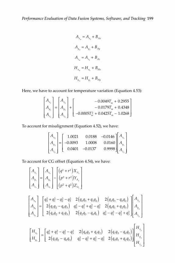
Performance Evaluation of Data Fusion Systems, Software, and Tracking 199

Axm

= Ax3+ BAx

Aym

= Ay3+ BAy

Azm

= Az3+ BAz

Hxm

= Hxb+ BHx

Hym

= Hyb+ BHy

Here, we have to account for temperature variation (Equation 4.53):

Ax3

Ay3

Az3

⎡

⎣

⎢⎢⎢⎢

⎤

⎦

⎥⎥⎥⎥

=

Ax2

Ay2

Az2

⎡

⎣

⎢⎢⎢⎢

⎤

⎦

⎥⎥⎥⎥

+ − 0.0049Tm + 0.2955

− 0.0179Tm + 0.4348

−0.0005Tm2 + 0.0425Tm − 1.0268

⎡

⎣

⎢⎢⎢

⎤

⎦

⎥⎥⎥

To account for misalignment (Equation 4.52), we have:

Ax2

Ay2

Az2

⎡

⎣

⎢⎢⎢⎢

⎤

⎦

⎥⎥⎥⎥

= 1.0021 0.0188 −0.0146

−0.0093 1.0008 0.0160

0.0401 −0.0137 0.9998

⎡

⎣

⎢⎢⎢

⎤

⎦

⎥⎥⎥

Ax1

Ay1

Az1

⎡

⎣

⎢⎢⎢⎢

⎤

⎦

⎥⎥⎥⎥

To account for CG offset (Equation 4.54), we have:

Ax1

Ay1

Az1

⎡

⎣

⎢⎢⎢⎢

⎤

⎦

⎥⎥⎥⎥

=

Axb

Ayb

Azb

⎡

⎣

⎢⎢⎢⎢

⎤

⎦

⎥⎥⎥⎥

−

q2 + r2( )XAx

p2 + r2( )YAy

p2 + q2( )ZAz

⎡

⎣

⎢⎢⎢⎢

⎤

⎦

⎥⎥⎥⎥

Axb

Ayb

Azb

⎡

⎣

⎢⎢⎢⎢

⎤

⎦

⎥⎥⎥⎥

=

q02 + q1

2 − q22 − q3

2 2 q0q3 + q1q2( ) 2 q1q3 − q0q2( )2 q1q2 − q0q3( ) q0

2 − q12 + q2

2 − q32 2 q0q1 + q2q3( )

2 q0q2 + q1q3( ) 2 q2q3 − q0q1( ) q02 − q1

2 − q22 + q3

2

⎡

⎣

⎢⎢⎢

⎤

⎦

⎥⎥⎥

Axg

Ayg

Azg

⎡

⎣

⎢⎢⎢⎢

⎤

⎦

⎥⎥⎥⎥

Hxb

Hyb

⎡

⎣⎢⎢

⎤

⎦⎥⎥=

q02 + q1

2 − q22 − q3

2 2 q0q3 + q1q2( ) 2 q1q3 − q0q2( )2 q1q2 − q0q3( ) q0

2 − q12 + q2

2 − q32 2 q0q1 + q2q3( )

⎡

⎣⎢⎢

⎤

⎦⎥⎥

Hxg

Hyg

Hzg

⎡

⎣

⎢⎢⎢⎢

⎤

⎦

⎥⎥⎥⎥

200 Multi-Sensor Data Fusion: Theory and Practice

Although the sensor models are derived accurately from the calibration data, additional states are provided in the KF model to account for errors in the sensor model, such as sensor bias. The fi rst observable element (also known as measurement variable) in the measurement model is the quater-nion constraint equation [83]. It contains the quaternion states in the range of −1 to +1 and eases the scaling problems in the computation. It is assigned the highest priority by assigning a low measurement covariance.

Filter performance, with the attitudes changing at a rate of 0.1 rad/ second, and the fi lter update time of 0.1 second were obtained; although it gave a reasonably good performance when it was implemented on the microcontroller, the performance deteriorated, mainly because of the slower computational speed of the microcontroller (16 MHz clock speed). With the 12-state model, each update cycle on the microcontroller took nearly 2 seconds. Also, because the system was nonlinear, the fi lter perfor-mance deteriorated when the fi lter update rate was slow. To have a faster fi lter update, the fi lter model size was reduced from 12-state to 4-state, retaining only the quaternion states with an assumption that the sen-sor model is accurate enough. The estimates from the 12-state model and the 4-state model were reasonably close. This showed the validity of the 4-state model because it estimates attitudes reasonably well. Complete results are presented in [78]. Hence, only the 4-state model was imple-mented on the microcontroller, and it models the sensors as accurately as possible, reducing the unaccounted bias in their outputs.

4.5.4 Microcontroller Implementation

The outputs of rate gyros, accelerometers, and temperature sensors are analog and are acquired through a 12-bit ADC; an assembly code was developed to acquire the ADC output data. The magnetometer V2X, which is operational in raw mode, gives the digital output and hence was connected directly to the HC12 compact. The magnetometer gives out the data after certain events take place at certain intervals of time. The EKF algorithm was implemented in U-D factorization form, which was coded in embedded C programming. The EKF code, before implementation on the microcontroller, was compiled using PC compiler Borland C++, executed, and tested to reproduce the results obtained from MATLAB/Simulink to ensure that there were no errors in fi lter code conversion from MATLAB to C. The rate outputs from the gyros, accelerometers, and temperature transducer were acquired via ADC by including the relevant assembly code. All the fi les were compiled to a machine code using an Image Crafts C (ICC12) compiler [84]. This compiled M/C language code was downloaded onto the microcontroller using TwinPEEKs monitor program [85] residing in the internal EEPROM of the HC12 compact. The ADC outputs acquired were in 12-bit resolution and were converted into

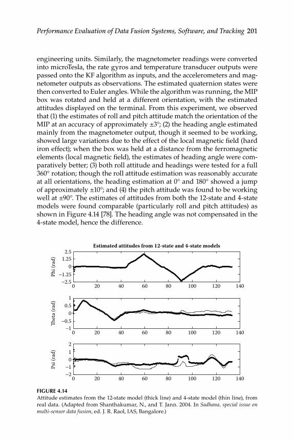
Performance Evaluation of Data Fusion Systems, Software, and Tracking 201

engineering units. Similarly, the magnetometer readings were converted into microTesla, the rate gyros and temperature transducer outputs were passed onto the KF algorithm as inputs, and the accelerometers and mag-netometer outputs as observations. The estimated quaternion states were then converted to Euler angles. While the algorithm was running, the MIP box was rotated and held at a different orientation, with the estimated attitudes displayed on the terminal. From this experiment, we observed that (1) the estimates of roll and pitch attitude match the orientation of the MIP at an accuracy of approximately ±3°; (2) the heading angle estimated mainly from the magnetometer output, though it seemed to be working, showed large variations due to the effect of the local magnetic fi eld (hard iron effect); when the box was held at a distance from the ferromagnetic elements (local magnetic fi eld), the estimates of heading angle were com-paratively better; (3) both roll attitude and headings were tested for a full 360° rotation; though the roll attitude estimation was reasonably accurate at all orientations, the heading estimation at 0° and 180° showed a jump of approximately ±10°; and (4) the pitch attitude was found to be working well at ±90°. The estimates of attitudes from both the 12-state and 4-state models were found comparable (particularly roll and pitch attitudes) as shown in Figure 4.14 [78]. The heading angle was not compensated in the 4-state model, hence the difference.

FIGURE 4.14 Attitude estimates from the 12-state model (thick line) and 4-state model (thin line), from

real data. (Adapted from Shanthakumar, N., and T. Jann. 2004. In Sadhana, special issue on multi-sensor data fusion, ed. J. R. Raol, IAS, Bangalore.)

−2.5−1.25

01.25

2.5Estimated attitudes from 12-state and 4-state models

Phi (

rad)

−1−0.5

00.5

1

Thet

a (ra

d)

0 20 40 60 80 100 120 140

0 20 40 60 80 100 120 140

0 20 40 60 80 100 120 140

−2−1

012

Psi (

rad)

203

Epilogue

Reference 86 gives the fusion equations for the state-vector fusion process when common process noise is present in the system. It gives analytical evaluations of the possible effects on data fusion due to such noise, which are ignored in many studies. [87] is one of the earliest satisfactory books on mathematics in data fusion. Work on the evaluation of the H-I fi lters for systems of the state-vector dimension higher than two (i.e., to include the acceleration state of the moving object) and more than two sensors would be very interesting. Future work could be pursued in the validation of these fusion algorithms with real data from practical applications such as tracking problems, decentralized estimations and control of fl exible struc-tures, and mechatronics. Some discussion on data association and fusion algorithms for tracking in the presence of measurement loss can be found in reference 88. Research on the use of multisensor data fusion for sensor failure detection and health monitoring systems is gradually catching up (reference 89 is just an indication). A direct approach to data fusion that estimates the joint distribution of just the variables of interests is presented in reference 90. This approach yields solutions that can be implemented along with conventional statistical models. Interestingly, for marketing applications, it considers variables such as common psychographic and demographic data and the variables to be fused such as media viewing and product purchases. However, the common variables are not used for the estimation of the joint distribution of the fusion variables. “Pooling information” methods can be used for data fusion and decision fusion, as well as for incorporating “reliability” into the fusion process (see Appen-dix). Some details and development related to data association and inter-active multiple model applications can be found in references 91 and 92.

Exercises

I.1. What is the motivation for sensor fusion and what are the general merits and demerits of a multiple sensor suit for data fusion?

I.2. Give specifi c names for the advantages of sensor data fusion system. (Hint: e.g., robust performance.)

I.3. What are the specifi c merits and demerits of various sensor data fusion models (Section 2.1)?

204 Multi-Sensor Data Fusion: Theory and Practice

I.4. What are the merits and demerits of sensor-network confi gura-tions and architectures?

I.5. What is the fundamental difference between the weighted LS and KF per se and how are they different from the sensor data fusion point of view?

I.6. In state-vector fusion, is it necessary to invoke the cross-covariance between KFs for fusion? Why or why not?

I.7. What are the merits of using the Bayesian approach for fusion as well as for parameter/state estimation?

I.8. Which fusion method, the data level or the state- vector level, will generally be more accurate?

I.9. Which part of the KF can be regarded as very similar to the recursive least-squares (RLS) algorithm?

I.10. What are the merits of a factorization approach for fi ltering compared to the basic KF algorithm?

I.11. Establish by simple algebraic steps the relationship between the fusion equations from covariance-state and information-state points of view.

I.12. What are the possible failure states of the sensor suit and actuator suit?

I.13. How can these failures be detected and identifi ed?

I.14. In a sensor data fusion system, one cannot actually improve the accuracy of any single or all sensors. Why not?

I.15. Regarding Exercise I.14, what is really meant by saying that the sensor data fusion improves the accuracy of the overall system? (When fusion is performed, people say they have obtained more accurate results.)

I.16. What is the distinction between sensor fusion and data fusion?

I.17. What are data fusion functions?

I.18. List some military and civilian applications of MSDF.

I.19. Sequence through the data acquisition chain from energy to the acquired knowledge.

I.20. How is the utility of the data fusion system measured?

I.21. What is the traditional view of the KF?

I.22. What is a Bayesian network? What is the use of a dynamic Bayesian network (DBN)?

I.23. What are the constraints of a decentralized data fusion system (DDFS)?

I.24. What are the specifi c characteristics of a DDFS?

Performance Evaluation of Data Fusion Systems, Software, and Tracking 205

I.25. Is fusion only an additive process? Or could it be otherwise?

I.26. Derive from fi rst principle the state-level fusion expression (refer Section 3.1.1) using the estimated states from two chan-nels and associated covariance matrices as the weighting fac-tors. (Hint: A good estimate would have a smaller covariance and should be given a greater weighting—that could be sup-plied by the not-so-good estimate!)

I.27. What are the kinematic and dynamic constraints of a mobile sensor platform?

I.28. What are the merits of square-root information fi lter (SRIF) when compared to the information fi lter (IF)?

I.29. How is a model transition matrix for the IMM-based fi lter for tracking a maneuvering target decided?

I. 30. When measurements are converted, why and how are their sta-tistics affected?

I.31. How could some errors creep into the fusion process?

I.32. What is the use of so-called sensor integration functions? (Hint: abstract sensors.)

I.33. What is the advantage gained by the fusion of data from a millimeter-wave radar (MMWR) and IR image?

I.34. Generate simulated (noisy) data using the state and measure-ment models of Equations 3.6 and 3.7 for two sensors in MAT-LAB using ftype = 1 (for KFA) and mdata = 1 (with measurement loss in sensor 1), in the MATLAB SW provided with the MSDF book. Use the measured data in a KF and perform state estima-tion using Equations 3.8 through 3.12 and state-vector fusion using Equations 3.13 and 3.14. Plot position and velocity (state) errors within their theoretical bounds.

I.35. Generate simulated (noisy) data using the state and measure-ment models of Equation 3.6 and 3.7 for two sensors in MAT-LAB using ftype = 2 (for GFA) and mdata = 1 (with measurement loss in sensor 1). Use the measured data in GFA and perform both state estimation and fusion using Equations 3.142 through 3.149. Plot position and velocity (state) errors within their theo-retical bounds. Observe the difference between the results of Exercise I.34 and this one.

I.36. Generate simulated (noisy) data using the state and measure-ment models of Equations 3.6 and 3.7 for two sensors in MAT-LAB (with measurement loss in sensor 2). Use the measured data in H-infi nity a posteriori estimation (fi ltering) algorithm and per-form state estimation using Equations 3.153 through 3.156 and

206 Multi-Sensor Data Fusion: Theory and Practice

state-vector fusion using Equations 3.157 and 3.158. Plot position and velocity (state) errors within their theoretical bounds.

I.37. Derive the standard BLUE estimation rule from the equations of the BLUE FR with a priori knowledge. What assumption is required?

I.38. If the standard deviation of the angular error of the radar is σar and the current estimated range is ρrr, then what is the variance of the radar range? What is the signifi cance of this relationship?

I.39. What are the background noise sources?

I.40. What is a false alarm?

I.41. What are the probable sources of a false alarm?

I.42. Why is faster data and scan sampling required in target tracking?

I.43. When does an observation satisfy the gate of a given track?

I.44. What is the relation between the Fisher information matrix and the KF covariance matrix?

I.45. What is the merit of the IF compared to the KF?

I.46. What are the features of clutter?

I.47. How might clutter be related to the false alarm?

I.48. What are the major differences between the NNKF, PDAF, and the strongest neighbor KF (SNKF) data association algorithms?

I.49. What is the major problem with NNKF?

I.50. How does PDAF try to circumvent this problem with NNKF (see Exercise I.49)?

I.51. How would you obtain the formulae for optimal WLS FR from the generalized weighted least-squares fusion rule?

References

1. Wilfried, E. 2002. An introduction to sensor fusion. Research report 47/2001 . Austria: Institute fur Technische Informatik, Vienna University of Technology.

2. Abidi, M. A., and R. C. Gonzalez, eds. 1992. Data fusion in robotics and machine intelligence . USA: Academic Press.

3. Dasarathy, B. V. 2001. Information fusion—what, where, why, when, and how? (Editorial) Inf Fusion 2:75−6.

4. Hall, D. L. 1992. Mathematical techniques in multi-sensor data fusion . Norwood, MA: Artech House.

Performance Evaluation of Data Fusion Systems, Software, and Tracking 207

5. Grossmann, P. 1998. Multisensor data fusion. GEC J Technol 15:27−37. 6. Nahin, P. J., and J. L. Pokoski. 1980. NCTR plus sensor fusion equals IFFN or

can two plus two equal fi ve? IEEE Trans Aerosp Electron Syst 16:320−37. 7. Dasarathy, B. V. 2000. More the merrier ... or is it? Sensor suite augmenta-

tion benefi ts assessment. In: Proceedings of the 3rd International Conference on Information Fusion , 2: 20−25. Paris, France.

8. Mutambra, A. G. O. 1998. Decentralized estimation and control for multisensor systems . Florida, USA: CRC Press.

9. Dasarathy, B. V. 2000. Industrial applications of multi-sensor information fusion. Proceedings of IEEE International Conference on Industrial Technology , Goa, India (Invited Plenary Session Talk).

10. Markin, M., C. Harris, M. Bernhardt, J. Austin, M. Bedworth, P. Greenway, R. Johnston, et al. 1997. Technology foresight on data fusion and data processing. Publication of The Royal Aeronautical Society.

11. Shulsky, A. N. 1991. Silent warfare: Understanding the world of intelligence . New York: Brassey’s.

12. Boyd, J. R. 1987. A discourse on winning and losing . Maxwell AFB, Alabama: Unpublished set of briefi ng slides available at Air University Library.

13. Bedworth, M. D., and J. O’Brien. 1999. The omnibus model: A new archi-tecture for data fusion? In Proceedings of the 2nd International Conference on Information Fusion (FUSION’99).

14. Raol, J. R., G. Girija, and J. Singh. 2004. Modelling and parameter estimation of dynamic systems (IEE control engg,) Vol. 65. London: IEE.

15. Rong Li, X., Y. M. Zhu, and C. Z. Han. Unifi ed optimal linear estimation fusion—Part I: Unifi ed models and fusion rules. In Proceedings of 2000 International Conference on Information Fusion, MoC2.10−MoC2.17, Paris, France.

16. Rong Li, X., and J. Wang. 2000. Unifi ed optimal linear estimation fusion—Part II: Discussions and examples. In Proceedings of 2000 International confer-ence on information fusion, MoC2.10−MoC2.17, Paris, France.

17. Rong Li, X., and P. Zhang. Optimal linear estimation fusion—Part III: Cross-correlation of local estimation errors. In Proceedings of 2000 International Conference on Information Fusion, WeB1.11–WeB1.18, Montreal, QC, Canada .

18. Rong Li, X., and K. Zhang. Optimal linear estimation fusion—Part IV: Optimality and effi ciency of distributed fusion. In Proceedings of 2000 International Conference on Information Fusion, WeB1.19–WeB1.26, Montreal, QC, Canada .

19. Rong Li, X., K. Zhang, J. Zhao, and Y. M. Zhu. 2002. Optimal linear esti-mation fusion—Part V: Relationships. Proceedings of 5th International Conf. Information Fusion , 497−504, Annapolis, MD, USA.

20. Dempster, A. P. 1967. Upper and lower probabilities induced by a multi- valued mapping. Annu Math Stat 38:325−39.

21. Shafer, G. 1976. A mathematical theory of evidence . Princeton, NJ: Princeton University Press.

22. Provan, G. M. 1992. The validity of Dempster–Shafer belief functions. Int J Approx Reason 6:389−99.

23. Crowley, J. L., and Y. Demazeu. 1993. Principles and techniques of sensor data fusion. Signal Processing, 32(2):5–27.

208 Multi-Sensor Data Fusion: Theory and Practice

24. Challa, S., and D. Koks. 2004. Bayesian and Dempster–Shafer fusion. Sadhana 29(2):145−76.

25. Kadambe, S., and C. Daniell. Sensor/data fusion based on value of informa-tion. In Proceedings of the Sixth International Conference on Information Fusion, 1:25–32.

26. Leung, L. W., B. King, and V. Vohora. 2001. Comparison of image data fusion techniques using entropy and INI. In Proceedings of the 22nd Asian confer-ence on remote sensing, Singapore, November 5–9. http://www.pubs.drdc.gc.ca/inbasket/Laidman.071121_1403.toronto_CR_2007_066.pdf. Accessed December 2008.

27. Iyengar, S. S., and R. R. Brooks, eds. 2005. Distributed sensor networks . Boca Raton, FL: Chapman & Hall/CRC Press.

28. Aggarwal, J. K., ed. 1993. Multisensor fusion for computer vision, NATO ASI Series . Berlin: Springer-Verlag.

29. Hu, H., and J. Q. Gan. 2005. Sensors and data fusion algorithms in mobile robotics. TR CSM-422, Dept. of Comp. Science, University of Essex, UK.

30. Vaghi, A. 2003–2004. Sensor management by a graphical model approach. Thesis, Politecnico di Milano. http://www. fred.mems.duke.edu/posters/Alberto_GMA_thesis.pdf. Accessed December 2008.

31. Manyika, J., and H. Durrant-Whyte. 1994. Data fusion and sensor management—decentralized information theoretic approach . New York: Ellis Horwood Series.

32. Maybeck, P. S. 1982. Stochastic models, estimation and control , Vol. 2. New York: Academic Press.

33. Bierman, G. J. 1977. Factorization methods for discrete sequential estimation . New York: Academic Press.

34. Julier, S. J., and J. K. Uhlmann. 1997. A new extension of the Kalman fi lter to non-linear systems. In Proceedings of AeroSense, 11th International Symposium Aerospace/Defense Sensing, Simulation and Controls . Bellingham, WA: SPIE.

35. Julier, S. J., and J. K. Uhlmann. 2004. Unscented fi ltering and non-linear estimation. Proc IEEE 92(3):401−22.

36. Kashyap, S. K., and J. R. Raol. 2006. Evaluation of derivative free Kalman fi l-ter and fusion in non-linear estimation . Ottawa, ON, Canada: IEEE Canadian Conference on Electrical and Computer Engineering.

37. Kashyap, S. K., and J. R. Raol. 2008. Evaluation of derivative free Kalman fi l-ter for non-linear state-parameter estimation and fusion. J Aeronaut Soc India 60(2):101−14.

38. Bar Shalom, Y., and X. R. Li. 1995. Multitarget–multisensor tracking: Principles and techniques . Storrs, CT: Academic Press.

39. Blackman, S. S. 1986. Multiple-target tracking with radar applications . Norwood, MA: Artech House.

40. Naidu, V. P. S., G. Girija, and J. R. Raol. 2005. Data association and fusion algo-rithms for tracking in presence of measurement loss. J Inst Eng I AS 86:17−28.

41. Chang, K. C., and Y. Bar-Shalom. 1994. FUSEDAT: A software package for fusion and data association and tracking with multiple sensors. In Proceedings of the SPIE conference on signal and data processing of small targets, Orlando, FL.

42. Mori, S., W. H. Barker, C.-Y. Chong, and K.-C. Chang. 2002. Track association and track fusion with nondeterministic target dynamics. IEEE Trans Aerosp Electron Syst 38(2):659–668.

Performance Evaluation of Data Fusion Systems, Software, and Tracking 209

43. Bar-Shalom, Y., and X.-R. Li. 1993. Estimation and tracking: Principles, techniques, and software. Boston, MA: Artech House.

44. Haimovich, A. M., J. Yosko, R. J. Greenberg, and M. A. Parisi. Fusion of sensors with dissimilar measurements/tracking accuracies. IEEE Log No. T-AES/29/1/02258.

45. Shanthakumar, N., and G. Girija. 2007. Measurement level and state-vector data fusion implementations. Personal communications and personal notes. Flight Mechanics and Control Division, National Aerospace Laboratories, Bangalore.

46. Kashyap, S. K., N. Shanthakumar, G. Girija, and J. R. Raol. 2003. Sensor data characterization and fusion for target tracking applications. International Radar Symposium India (IRSI), 3–5 December. Bangalore.

47. Zhou, Y., H. Leung, and M. Blanchette. 1999. Sensor alignment with earth-centered earth-fi xed co-ordinate system. IEE Trans AES 35(2):410−8.

48. Raol, J. R., and G. Girija. 2002. Sensor data fusion algorithms using square-root information fi ltering. IEE Proc Radar Sonar Navig 149(2):89−96.

49. Bar-Shalom, Y. and X.-R. Li. 1993. Estimation and tracking: Principles, techniques and software . Boston: Artech House.

50. Blom, H. A. P., and Y. Bar-Shalom. 1988. The interacting multiple model algo-rithm for systems with markovian switching coeffi cients. IEEE Trans Autom Control 33:780−3.

51. Mazor, E., A. Averbuch, Y. Bar-Shalom, and J. Dayan. 1998. Interacting mul-tiple model methods in target tracking: A survey. IEEE Trans Aerosp Electron Syst 34:103−23.

52. Naidu, V. P. S., G. Girija, and N. Santhakumar. 2007. Three model IMM-EKF for tracking targets executing evasive maneuvers. AIAA-66928, 45th AIAA conference on Aerospace Sciences, Reno, USA.

53. Simeonova, L., and T. Semerdjiev. 2002. Specifi c features of IMM tracking fi lter design. Inf Secur Int J 9:154−65.

54. Schulz, D., W. Burgard, D. Fox, and A. B. Cremers. People tracking with mobile robots using sample-based joint probabilistic data association fi lters. http://www.informatik.unibonn.de/~schulz/articles/people-tracking-ijrr-03.pdf.

55. Challa, S., R. J. Evans, and X. Wang. 2003. A Bayesian solution and its approx-imations to out-of-sequence measurement problems. Inf Fusion 4(3):185−99.

56. Paik, B. S., and J. H. Oh. 2000. Gain fusion algorithm for decentralized paral-lel Kalman fi lters. IEE Proc Control Theor App 147(1):97–103.

57. Shanthakumar, N., G. Girija, and J. R. Raol. 2001. Performance of Kalman and gain fusion algorithms for sensor data fusion with measurement loss. International Radar Symposium India (IRSI), Bangalore.

58. Green, M., and D. J. N. Limebeer. 1995. Linear robust control . Englewood Cliffs, NJ: Prentice Hall.

59. Hassibi, B., A. H. Sayad, and T. Kailath. 1996. Linear estimation in Krein spaces—part II: Applications. IEEE Trans Autom Control 41(1):34–49.

60. Jin, S. H., J. B. Park, K. K. Kim, and T. S. Yoon. 2001. Krein space approach to decentralized H ∞ state estimation. IEE Proc Control Theor App 148(6):502−8.

61. Lee, T. H., W. S. Ra, T. S. Yoon, and J. B. Park. 2004. Robust Kalman fi ltering via Krein space estimation. IEE Proc Control Theor App 151(1):59−63.

210 Multi-Sensor Data Fusion: Theory and Practice

62. Raol, J. R., and F. Ionescu. 2002. Performance of H-Infi nity fi lter-based data fusion algorithm with outliers. 40th AIAA Aerospace Sciences Meeting & Exhibit, 14–17 January 2002, Reno, NV, USA, A02-13598.

63. Ananthasayanam, M. R., A. K. Sarkar, A. Bhattacharya, P. Tiwari, and P. Vorha. 2005. Nonlinear observer state estimation from seeker measurements and seeker-radar measurements fusion, Paper No AIAA-2005-6066-CP.

64. Zarchan, P. 1997. Tactical and strategic missile guidance , Vol. 176, 3rd ed. Progress in Aeronautics and Astronautics.

65. Bar-Shalom, Y., and K. C. Chang. 1989. Tracking a maneuvering target using input estimation versus the interacting multiple model algorithm. IEEE Trans Aerosp Electron Syst 26(2):296–300.

66. Mehrotra, K., and P. Mahapatra. 1997. A jerk model for tracking highly maneuvering targets. IEEE Trans Aerosp Electron Syst 33(4):1094−105.

67. Vora, P., A. Bhattacharyya, M. Jyothi, P. K. Tiwari, and R. N. Bhattacharjee. 2004. RF Seeker modeling and Seeker fi lter design . Hyderabad, India: National Workshop on Tactical Missile Guidance.

68. Kashyap , S. K., N. Shanthakumar, V. P. S. Naidu, G. Girija, and J. R. Raol. 2007. State estimation for Pursuer guidance using interacting multiple model based augmented extended Kalman fi lter . International Radar Symposium, India, (IRSI) Bangalore.

69. Banerjee, P., and R. Appavu Raj. 2000. Multi-sensor data fusion strategies for real-time application in test and evaluation of rockets/missiles system. IEEE International Conference on Industrial Technology (ICIT), Goa, India.

70. Girija, G., J. R. Raol, R. Appavu Raj, and S. Kashyap. 2000. Tracking fi lter and multi-sensor data fusion. In Special issue: Advances in Modeling, System Identifi cation, and Parameter Estimation, eds. J. R. Raol and N. K. Sinha, Sadhana 25(2):159−67.

71. Kashyap, S. K., V. P. S. Naidu, J. Singh, G. Girija, and J. R. Raol. 2006. Tracking of multiple targets using interactive multiple model and data association fi l-ter. J Aerosp Sci Technol Aeronaut Soc India 58(1):65−74.

72. Lerro, D., and Y. Bar-Shalom. 1993. Tracking with de-biased consistent converted measurements versus EKF. IEEE Trans Aerosp Electron Syst 29(3):1015–1022.

73. Park, S.-T., and J. Gyu Lee. 2001. Improved Kalman fi lter design for three-dimension radar tracking. IEEE Trans Aerosp Electron Syst 37(2):727–739.

74. Blackman, S. 1986. Multiple target tracking with radar applications . Dedham, MA: Artech House.

75. Kashyap, S. K., G. Girija, and J. R. Raol. 2003. Evaluation of converted measurement- and modifi ed extended-Kalman fi lters for target tracking. AIAA Conference and Exhibit, Guidance, Navigation and Control, Texas, US, 11–17th August.

76. Kashyap, S. K., G. Girija, and J. R. Raol. 2006. Converted measurement- and modifi ed extended-Kalman fi lter for target tracking. Def Sci J 56(5):679−92.

77. Peter, S. 1979. Maybeck, stochastic models, estimation and control , Vol. 1. New York: Academic Press.

78. Shanthakumar, N., and T. Jann. 2004. Estimation of attitudes from a low cost miniaturized inertial platform using Kalman fi lter based sensor fusion algo-rithm. In Sadhana, special issue on multi-sensor data fusion, ed. J. R. Raol, IAS, Bangalore.

Performance Evaluation of Data Fusion Systems, Software, and Tracking 211

79. Doherr, K. F., and T. Jann. 1997. Test vehicle ALEX for low cost autonomous parafoil landing experiments. 14th AIAA Aerodynamic Decelerator Systems Technology Conference and Seminar, USA, AIAA-97-1543.

80. Jann, T., K. F. Doherr, and W. Gockel. Parafoil test vehicle ALEX- further development and fl ight test results, AIAA-99-1751.

81. Jann, T. 2001. Aerodynamic model identifi cation and GNC design for the Parafoil-Load system ALEX. Proccedings of AIAA Aerodynamic Systems Decelerator Conference , USA, AIAA-2001-2015.

82. Valvano, J. W. 2000. Embedded microcomputer systems . USA: Brooks/Cole. 83. Collinson, R. P. G. 1998. Introduction to avionics . UK: Chapman and Hall. 84. Anonymous. 2002. ImageCraft C compiler and development environment

for motorola HC12 manual, version 6. 85. Anonymous. 1999. HC12Compact hardware manual, Version 1.0. 86. Saha, R. K. 1996. Effect of common process noise on two-sensor track fusion.

J Guid Control Dyn 19(4):829–835. 87. Goodman, I. R., R. P. S. Mahler, and T. Hung. 1997. Mathematics of data fusion .

Norwell, MA: Kluwer. 88. Naidu, V. P. S., G. Girija, and J. R. Raol. 2003. Evaluation of data associa-

tion and fusion algorithms for tracking in the presence of measurement loss. AIAA Paper No. 5733, Austin (USA).

89. Girija, G., C. Zorn, and A. Koch. 2005. Multi sensor data fusion for sensor fail-ure detection and health monitoring. AIAA Guidance, Navigation and Control Conference and Exhibit, 15–18 Aug, AIAA-2005-5843, San Francisco, CA.

90. Gilula, Z., R. E. Mcculloch, and P. E. Rossi. 2006. A direct approach to data fusion. J Mark Res 43(1):73–83.

91. Girija, G., and J. R. Raol. 2001. Comparison of methods for association and fusion of multi-sensor data for tracking applications. AIAA Guidance, Navigation, and Control Conference and Exhibit. Montreal, Quebec, Canada. Paper No. AIAA-2001−4107, 6–9 August 2001.

92. Kashyap, S. K., V. P. S. N. Naidu, J. Singh, G. Girija, and J. R. Raol. 2004. Multiple target tracking using IMMPDAF fi lter. National Workshop on Tactical Guidance, DRDL, Hyderabad.

IIPart

Fuzzy Logic and Decision Fusion

J. R. Raol and S. K. Kashyap

215

5 Introduction

When we have multiple situations with several different analysis results, we often need to choose a situation or result that will lead us to our desired goal with reasonable accuracy. We need to use available knowledge and information as well as logic or a statistical method to arrive at an appropri-ate decision. Decision making is often (and perhaps always) coupled with knowledge representation, which is derived through an inference process or engine, operating with the measured data or collected raw information. In Part II, we emphasize the use of fuzzy logic (Type I FL/S; see Epilogue) for decision making and fusion.

Fuzzy logic (FL) has been understood for the last four decades [1]. Even before that, a third possibility beyond the “true” or “false” options given by binary logic might have been indicated. The third value can be translated as “possible,” with a numeric value between true and false, and there can be infi nite-valued logic possible to represent certain kind of uncertainty. Zadeh’s FL facilitates the modeling or representation of conditions that are inherently imprecisely defi ned. Fuzzy techniques (based on FL—the techniques in themselves may not be fuzzy), as a part of approximate reasoning, provide decision support and expert systems with reasoning capabilities. FL techniques have been used in various applications: (1) image-analysis, e.g. detection of edges, feature extraction, classifi cation, and clustering; (2) parameter estimation of unknown dynamic systems, e.g. aircraft; (3) home appliances, e.g. washing machines, air conditioning systems; (4) design of control systems; (5) sensor failure detection, identi-fi cation, and isolation; (6) reconfi guration control; and (7) decision fusion, e.g. situation and threat assessment [2–4]. FL has an inherent ability to approximately mimic the human mind so that it can be used for reasoning that is more approximate rather than exact.

In Part II, we will summarize FL concepts and their potential applica-tions in both engineering and nonengineering fi elds. Part II introduces FL concepts, fuzzy sets, membership functions for fuzzifi cation processes, fuzzy operators, fuzzy implication methods (FIM), aggregation methods, defuzzifi cation methods, and the steps of fuzzy inference engine, or pro-cess (FIE). It highlights: (1) the relationship between fuzzy operators such as T-norms and S-norms, (2) the interconnectivities of fuzzy operators and FIM, and (3) the contradistinctions among various operations using numerical simulation examples [3,5–7]. The use of FL in recursive state

216 Multi-Sensor Data Fusion: Theory and Practice

estimation and sensor data fusion is also considered. The algorithms are developed by considering the combination of FL and Kalman fi lter (KF). Two schemes, KF and fuzzy KF (FKF), are used for target-tracking applica-tions and the evaluation of performance. The concept of FL is extended to state-level data fusion for similar sensors. The performances of FL-based fusion methods are compared with the conventional fusion method, that is, state-vector fusion (SVF), to track a maneuvering target.

We will need to select an appropriate implication method from the existing methods. However, if any new implication method is found, it should satisfy some of the intuitive criteria of forward chain logic/gener-alized modus ponens (GMP) and backward chain logic/generalized modus tollens (GMT) so that it can be fi tted into the process of system develop-ment using FL. We will need to develop a procedure to fi nd out if any of the existing implication methods satisfi es the given set of intuitive criteria for GMP and GMT. To realize this scheme, MATLAB® and graphics have been used to develop a user-interactive package to evaluate implication methods with respect to these criteria [5,7]. The criteria of GMP/GMT [3,7] and the derivations and an explanation of various FIM are given. The steps required to interpret the implication methods with respect to these criteria are also given. Some new FIM are proposed and derived using material implications, propositional calculus, and fuzzy operators. These FIM are evaluated with GMP/GMT using MATLAB or a graphics-based tool, as referred to above. We will consider one situation in which decision fusion can be used: in the battlefi eld, where it can be used to determine a fi nal decision based on the entire surveillance volume at any time, using outputs from different levels, e.g., level 1—object refi nement, and level 2—situation refi nement of the multisensor data fusion (MSDF) system. This will include some examples of decision support systems realized using a MATLAB/Simulink® environment or MATLAB-based FL tool-box. These examples are only a part of the many situations that can be encountered in combat scenarios, such as air-to-air, air-to-ground, ground-to-air, and so on. A similar process is also applicable to other nonmilitary systems, but the details of the system would be different.

217

6Theory of Fuzzy Logic

Crisp logic is traditionally used in decision making and related analyses. The theory of probability is based on this logic, through the medium of classical set theory. In crisp logic, there are only two discrete states: “yes” or “no,” 0 or 1, –1 or +1, and “off” or “on.” There is no third possibility here—either a person is in the room or not, an event will occur on not, a light bulb is on or off, and so on. Real-life experiences prove that many more conditions than these two options are possible: the light could be dim, the day could be a certain degree of brightness or darkness, the weather could be warm, hot, hotter, or cold, very cold, and so on. This complexity necessitates variations in the degree of uncertainty, and hence, truth and falsity (1 or 0, respectively) are the two extremes of a continuous spectrum of uncertainty. This leads to multivalued logic and to fuzzy logic (FL)—a theory of sets wherein the characteristic function is generalized to assume an infi nite number of values between 0 and 1 (e.g., a triangular form). In fact, the theory of possibility [4] is based on FL, in a manner similar to the theory of probability, which is based on crisp logic (via set theory).

FL-based methods have found excellent applications in industrial control systems, home appliances, robotics, and aerospace engineering. The conventional control system can be regarded as a (minimally) intel-ligent-control system, if it uses FL (or any other logic) and/or any learn-ing mechanism. If, for example, y > some number, then use one controller or use another one—this is conditional logic. Essentially, artifi cial intel-ligence (AI)-based systems should have strong logical capability and very good learning and adaptive mechanisms. An FL-based controller is suited (1) to keep output variables between the limits; and (2) to maintain control actuation (i.e., control input or related variable) between the limits [2]. Thus, FL is a form of logic that can be used in the design and operation of an intelligent control. FL deals with vagueness, rather than uncertainty. For example, if a patient has a “severe” headache, then there is a “good chance” that she or he has a migraine. To avoid contradictions in the rules, a certain degree of human intervention is sometimes needed at certain stages to tune various adjustable parameters in the FL system (FLS) and rule base. FL-based control is suitable when (1) the control- system dynam-ics are slow and/or nonlinear; (2) the models of the plant are not available; and (3) competent human operators who can provide expert rules are available [2].

218 Multi-Sensor Data Fusion: Theory and Practice

The development of an FLS requires that the following tasks be accomplished: (1) select fuzzy sets and their membership functions for the fuzzifi cation process; (2) create a rule-base with the help of a domain expert, for input-output mapping; (3) select fuzzy operators in the fuzzy implica-tion and aggregation process; (4) select the fuzzy implication and aggrega-tion methods; and (5) select a defuzzifi cation method. The concepts of FL, fuzzy sets, their properties, FL operators, fuzzy proposition- and rule-based systems, fuzzy maps and inference engines, defuzzifi cation methods, and the evaluation of fuzzy implication functions are studied in this chapter.

6.1 Interpretation and Unification of Fuzzy Logic Operations

In this section, the relationships, interconnectivities, and contradistinc-tions among various operations and operators used in FLS [2–8] are explained using numerical simulations and examples.

6.1.1 Fuzzy Sets and Membership Functions

In principle, a fuzzy set is an internal extension or expansion of a crisp set, within the limits of the crisp set; hence, FL is richer than a crisp set (logic). A crisp set allows only full membership (1, an event occurred) or no membership at all (0, event did not occur), whereas a fuzzy set allows partial membership for a member of a set (belonging to the set). A crisp logic–membership function is defi ned as follows:

μA(u) =

1 if u ∈A

0 if u ∉A

⎧⎨⎩

(6.1)

Here, mA(u) is a membership function that characterizes the elements u of set A, in Figure 6.1.

A fuzzy set A based on a universe of discourse (UOD) U with elements u is expressed as

A = μA (u)/u{ }∫ ∀ u ∈U (6.2)

or A = μA(u)/u{ }∑ ∀ u ∈U (6.3)

Here, mA(u) is a membership function (a fuzzy membership function or FMF) of u in the set A and provides a mapping of UOD U in the closed

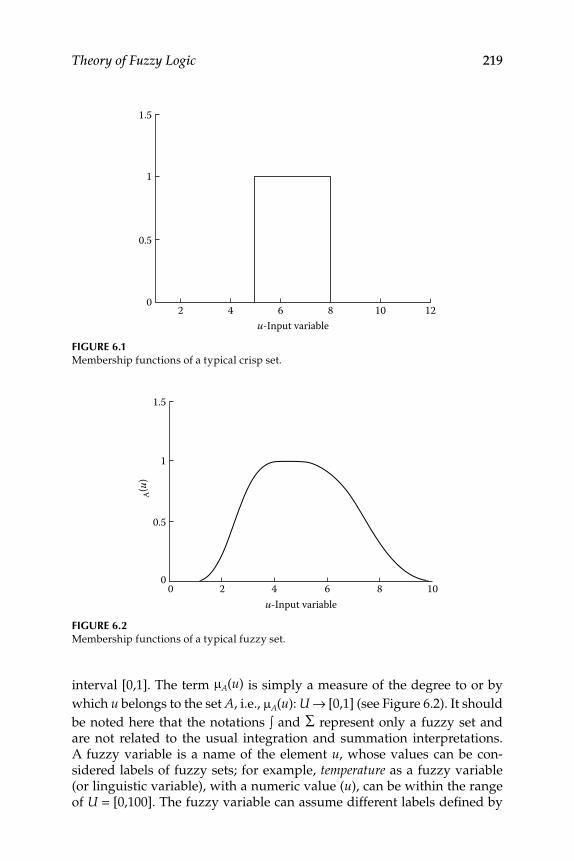
Theory of Fuzzy Logic 219

interval [0,1]. The term mA(u) is simply a measure of the degree to or by

which u belongs to the set A, i.e., mA(u): U → [0,1] (see Figure 6.2). It should

be noted here that the notations ∫ and ∑ represent only a fuzzy set and are not related to the usual integration and summation interpretations. A fuzzy variable is a name of the element u, whose values can be con-sidered labels of fuzzy sets; for example, temperature as a fuzzy variable (or linguistic variable), with a numeric value (u), can be within the range of U = [0,100]. The fuzzy variable can assume different labels defi ned by

1.5

1

0.5

02 4 6

u-Input variable8 10 12

FIGURE 6.1Membership functions of a typical crisp set.

FIGURE 6.2Membership functions of a typical fuzzy set.

1.5

1

0.5

00 2 4

u-Input variable

µ A(u

)

6 8 10

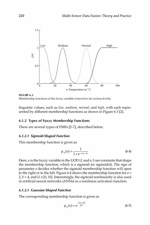
220 Multi-Sensor Data Fusion: Theory and Practice

linguistic values, such as low, medium, normal, and high, with each repre-sented by different membership functions as shown in Figure 6.3 [2].

6.1.2 Types of Fuzzy Membership Functions

There are several types of FMFs [2–7], described below.

6.1.2.1 Sigmoid-Shaped Function

This membership function is given as

μA(u) = 1

1+ e− a(u − b) (6.4)

Here, u is the fuzzy variable in the UOD U, and a, b are constants that shape the membership function, which is a sigmoid (or sigmoidal). The sign of parameter a decides whether the sigmoid membership function will open to the right or to the left. Figure 6.4 shows the membership function for a = 2, b = 4, and U ∈[0, 10]. Interestingly, the sigmoid nonlinearity is also used in artifi cial neural networks (ANNs) as a nonlinear activation function.

6.1.2.1 Gaussian-Shaped Function

The corresponding membership function is given as

μA(u) = e−(u − a)2

2b2 (6.5)

FIGURE 6.3Membership functions of the fuzzy variable temperature (at various levels).

1.5

1Low Medium Normal High

0.5

0 0 20 40u-Temperature in ˚C

µ A(u

)

60 80 100

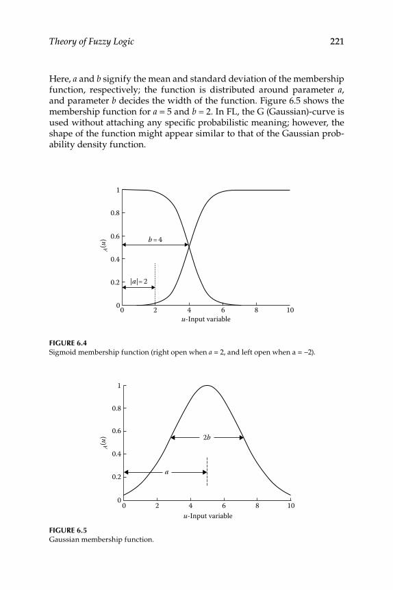
Theory of Fuzzy Logic 221

Here, a and b signify the mean and standard deviation of the membership function, respectively; the function is distributed around parameter a, and parameter b decides the width of the function. Figure 6.5 shows the membership function for a = 5 and b = 2. In FL, the G (Gaussian)-curve is used without attaching any specifi c probabilistic meaning; however, the shape of the function might appear similar to that of the Gaussian prob-ability density function.

FIGURE 6.4Sigmoid membership function (right open when a = 2, and left open when a = −2).

1

0.8

0.6 b = 4

|a|= 2

0.4

0.2

00 2 4 6u-Input variable

µ A(u

)

8 10

FIGURE 6.5Gaussian membership function.

1

0.8

2b

a

0.6

0.4

0.2

00 2 4

u-Input variable

µ A(u

)

6 8 10

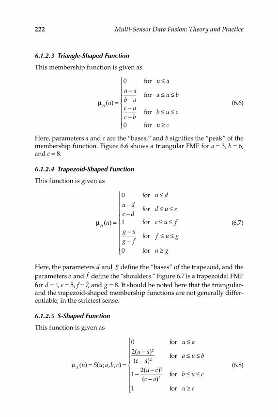
222 Multi-Sensor Data Fusion: Theory and Practice

6.1.2.3 Triangle-Shaped Function

This membership function is given as

μA (u) =

0 for u ≤ a

u − ab − a

for a ≤ u ≤ b

c − uc − b

for b ≤ u ≤ c

0 for u ≥ c

⎧

⎨

⎪⎪⎪

⎩

⎪⎪⎪

(6.6)

Here, parameters a and c are the “bases,” and b signifi es the “peak” of the membership function. Figure 6.6 shows a triangular FMF for a = 3, b = 6, and c = 8.

6.1.2.4 Trapezoid-Shaped Function

This function is given as

μA (u) =

0 for u ≤ d

u − de − d

for d ≤ u ≤ e

1 for e ≤ u ≤ f

g − ug − f

for f ≤ u ≤ g

0 for u ≥ g

⎧

⎨

⎪⎪⎪⎪

⎩

⎪⎪⎪⎪

(6.7)

Here, the parameters d and g defi ne the “bases” of the trapezoid, and the

parameters e and f defi ne the “shoulders.” Figure 6.7 is a trapezoidal FMF

for d = 1, e = 5, f = 7, and g = 8. It should be noted here that the triangular- and the trapezoid-shaped membership functions are not generally differ-entiable, in the strictest sense.

6.1.2.5 S-Shaped Function

This function is given as

μA (u) = S(u; a,b, c) =

0 for u ≤ a

2(u − a)2

(c − a)2for a ≤ u ≤ b

1 − 2(u − c)2

(c − a)2for b ≤ u ≤ c

1 for u ≥ c

⎧

⎨

⎪⎪⎪

⎩

⎪⎪⎪

(6.8)

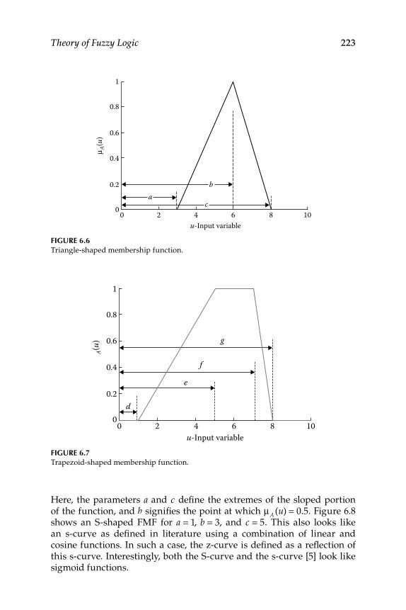
Theory of Fuzzy Logic 223

Here, the parameters a and c defi ne the extremes of the sloped portion of the function, and b signifi es the point at which μA (u) = 0.5. Figure 6.8 shows an S-shaped FMF for a = 1, b = 3, and c = 5. This also looks like an s-curve as defi ned in literature using a combination of linear and cosine functions. In such a case, the z-curve is defi ned as a refl ection of this s-curve. Interestingly, both the S-curve and the s-curve [5] look like sigmoid functions.

FIGURE 6.6Triangle-shaped membership function.

1

0.8

0.6

0.4

0.2

0 0 2

ab

c4

u-Input variable

µ A(u

)

6 8 10

FIGURE 6.7Trapezoid-shaped membership function.

1

0.8

0.6

0.4

0.2d

e

f

g

00 2 4

u-Input variable

µ A(u

)

6 8 10

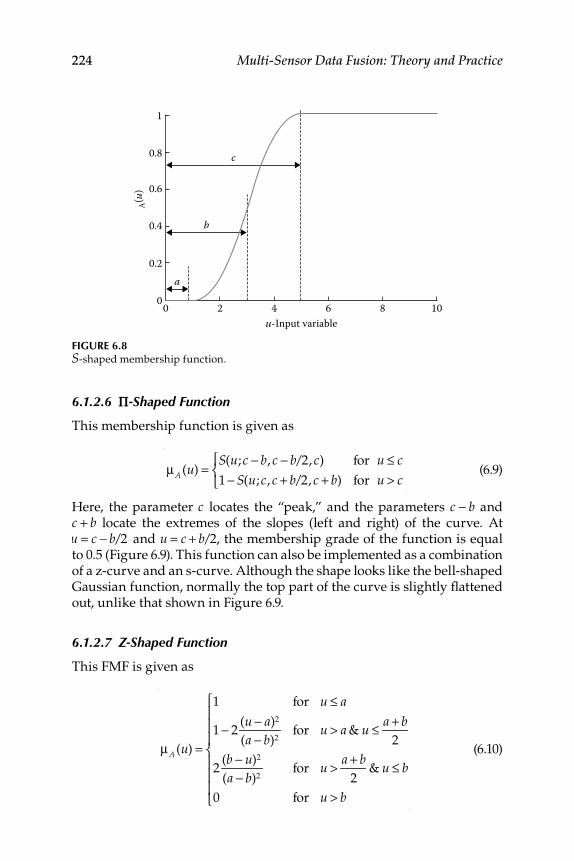
224 Multi-Sensor Data Fusion: Theory and Practice

6.1.2.6 Π-Shaped Function

This membership function is given as

μA (u) =

S(u;c − b, c − b/2, c) for u ≤ c

1 − S(u;c, c + b/2, c + b) for u > c

⎧⎨⎩

(6.9)

Here, the parameter c locates the “peak,” and the parameters c − b and c + b locate the extremes of the slopes (left and right) of the curve. At u = c − b/2 and u = c + b/2, the membership grade of the function is equal to 0.5 (Figure 6.9). This function can also be implemented as a combination of a z-curve and an s-curve. Although the shape looks like the bell-shaped Gaussian function, normally the top part of the curve is slightly fl attened out, unlike that shown in Figure 6.9.

6.1.2.7 Z-Shaped Function

This FMF is given as

μA (u) =

1 for u ≤ a

1 − 2(u − a)2

(a − b)2for u > a & u ≤ a + b

2

2(b − u)2

(a − b)2for u > a + b

2& u ≤ b

0 for u > b

⎧

⎨

⎪⎪⎪

⎩

⎪⎪⎪

(6.10)

FIGURE 6.8S-shaped membership function.

1

0.8

0.6

0.4

0.2

00 2 4 6

u-Input variable

a

b

c

µ A(u

)

8 10

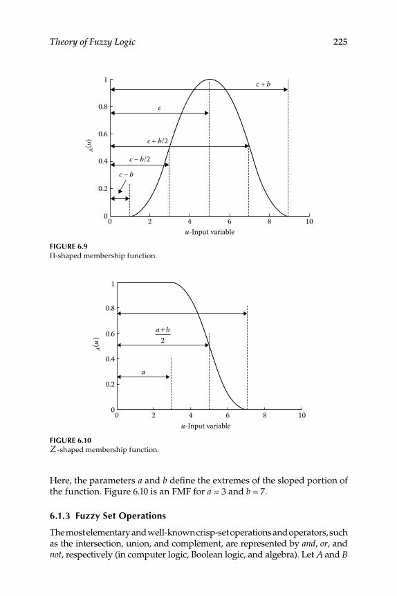
Theory of Fuzzy Logic 225

Here, the parameters a and b defi ne the extremes of the sloped portion of the function. Figure 6.10 is an FMF for a = 3 and b = 7.

6.1.3 Fuzzy Set Operations

The most elementary and well-known crisp-set operations and operators, such as the intersection, union, and complement, are represented by and, or, and not, respectively (in computer logic, Boolean logic, and algebra). Let A and B

FIGURE 6.9Π-shaped membership function.

1 c + b

c + b/2

c - b/2

c - b

c0.8

0.6

0.4

0.2

00 2 4

u-Input variable

µ A(u

)

6 8 10

FIGURE 6.10Z -shaped membership function.

1

0.8

0.6

0.4

a0.2

00 2 4 6

u-Input variable

µ A(u

)

8 10

a + b2

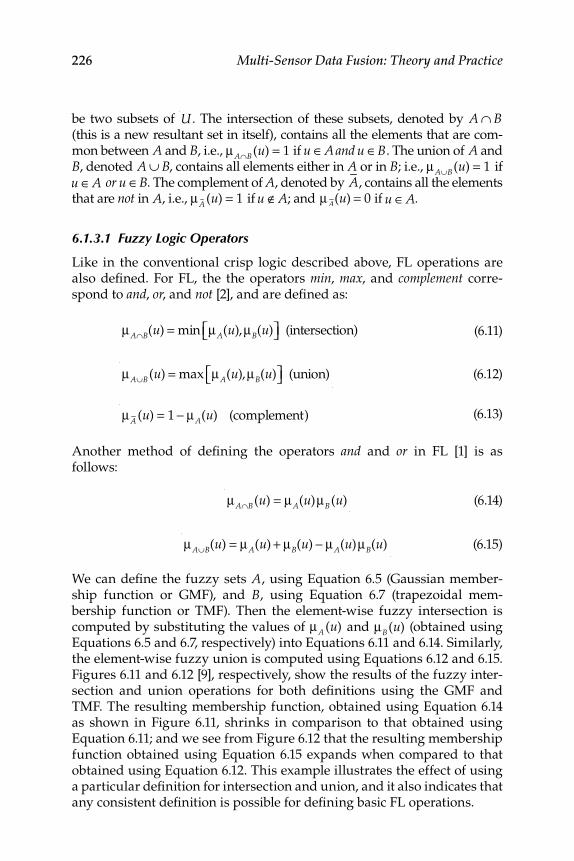
226 Multi-Sensor Data Fusion: Theory and Practice

be two subsets of U . The intersection of these subsets, denoted by A ∩ B (this is a new resultant set in itself), contains all the elements that are com-mon between A and B, i.e., μA∩B(u) = 1 if u ∈A and u ∈B. The union of A and B, denoted A ∪ B, contains all elements either in A or in B; i.e., μA∪B(u) = 1 if

u ∈A or u ∈B. The complement of A, denoted by A, contains all the elements that are not in A, i.e., μA (u) = 1 if u ∉A; and μA(u) = 0 if u ∈A.

6.1.3.1 Fuzzy Logic Operators

Like in the conventional crisp logic described above, FL operations are also defi ned. For FL, the the operators min, max, and complement corre-spond to and, or, and not [2], and are defi ned as:

μA∩B(u) = min μA(u),μB(u)⎡⎣ ⎤⎦ (intersection) (6.11)

μA∪B(u) = max μA(u),μB(u)⎡⎣ ⎤⎦ (union) (6.12)

μA (u) = 1 − μA(u) (complement) (6.13)

Another method of defi ning the operators and and or in FL [1] is as follows:

μA∩B(u) = μA(u)μB(u) (6.14)

μA∪B(u) = μA(u) + μB(u) − μA(u)μB(u) (6.15)

We can defi ne the fuzzy sets A, using Equation 6.5 (Gaussian member-ship function or GMF), and B, using Equation 6.7 (trapezoidal mem-bership function or TMF). Then the element-wise fuzzy intersection is computed by substituting the values of μA (u) and μB(u) (obtained using Equations 6.5 and 6.7, respectively) into Equations 6.11 and 6.14. Similarly, the element-wise fuzzy union is computed using Equations 6.12 and 6.15. Figures 6.11 and 6.12 [9], respectively, show the results of the fuzzy inter-section and union operations for both defi nitions using the GMF and TMF. The resulting membership function, obtained using Equation 6.14 as shown in Figure 6.11, shrinks in comparison to that obtained using Equation 6.11; and we see from Figure 6.12 that the resulting membership function obtained using Equation 6.15 expands when compared to that obtained using Equation 6.12. This example illustrates the effect of using a particular defi nition for intersection and union, and it also indicates that any consistent defi nition is possible for defi ning basic FL operations.

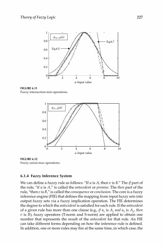
Theory of Fuzzy Logic 227

6.1.4 Fuzzy Inference System

We can defi ne a fuzzy rule as follows: “If u is A, then v is B.” The if part of the rule, “if u is A,” is called the antecedent or premise. The then part of the rule, “then v is B,” is called the consequence or conclusion. The core is a fuzzy inference engine (FIE) that defi nes the mapping from input fuzzy sets into output fuzzy sets via a fuzzy implication operation. The FIE determines the degree to which the antecedent is satisfi ed for each rule. If the antecedent of a given rule has more than one clause (e.g., if u1 is A

1 and u2 is A

2, then

v is B), fuzzy operators (T-norm and S-norm) are applied to obtain one number that represents the result of the antecedent for that rule. An FIE can take different forms depending on how the inference rule is defi ned. In addition, one or more rules may fi re at the same time, in which case, the

FIGURE 6.11Fuzzy intersection-min operations.

μA∩B(u)

u-Input value

00 2 4 6 8 10

0.2

0.4

0.6

0.8

1

Eq.6.5

Eq.6.7

FIGURE 6.12Fuzzy union-max operations.

u-Input value

1

0.8

0.6

0.4

0.2

00 2 4 6 8 10

μA∪B(u)

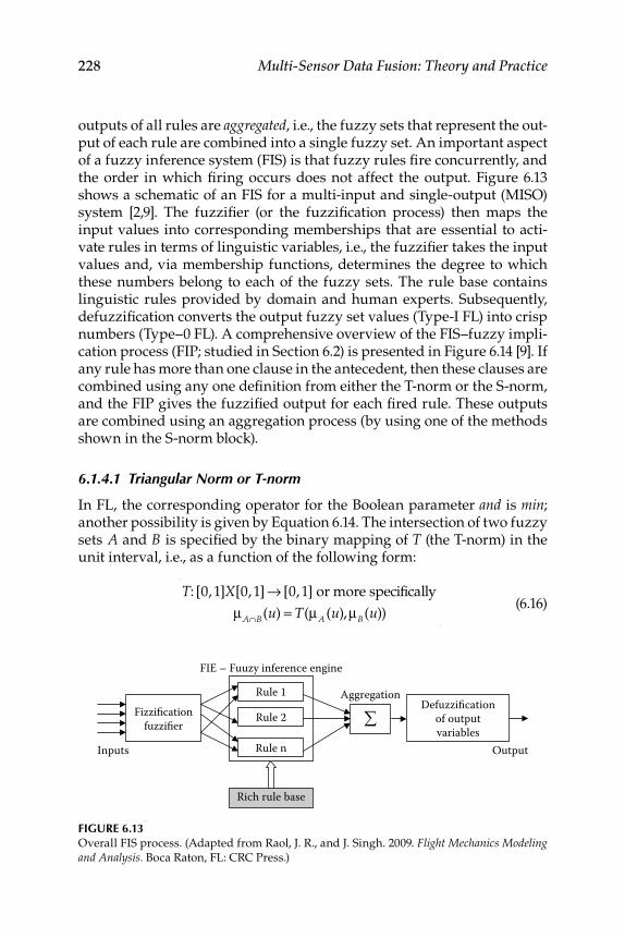
228 Multi-Sensor Data Fusion: Theory and Practice

outputs of all rules are aggregated, i.e., the fuzzy sets that represent the out-put of each rule are combined into a single fuzzy set. An important aspect of a fuzzy inference system (FIS) is that fuzzy rules fi re concurrently, and the order in which fi ring occurs does not affect the output. Figure 6.13 shows a schematic of an FIS for a multi-input and single-output (MISO) system [2,9]. The fuzzifi er (or the fuzzifi cation process) then maps the input values into corresponding memberships that are essential to acti-vate rules in terms of linguistic variables, i.e., the fuzzifi er takes the input values and, via membership functions, determines the degree to which these numbers belong to each of the fuzzy sets. The rule base contains linguistic rules provided by domain and human experts. Subsequently, defuzzifi cation converts the output fuzzy set values (Type-I FL) into crisp numbers (Type–0 FL). A comprehensive overview of the FIS–fuzzy impli-cation process (FIP; studied in Section 6.2) is presented in Figure 6.14 [9]. If any rule has more than one clause in the antecedent, then these clauses are combined using any one defi nition from either the T-norm or the S-norm, and the FIP gives the fuzzifi ed output for each fi red rule. These outputs are combined using an aggregation process (by using one of the methods shown in the S-norm block).

6.1.4.1 Triangular Norm or T-norm

In FL, the corresponding operator for the Boolean parameter and is min; another possibility is given by Equation 6.14. The intersection of two fuzzy sets A and B is specifi ed by the binary mapping of T (the T-norm) in the unit interval, i.e., as a function of the following form:

T: [0,1]X[0,1] → [0,1] or more specifically

μA∩B(u) = T(μA (u),μB(u)) (6.16)

FIGURE 6.13Overall FIS process. (Adapted from Raol, J. R., and J. Singh. 2009. Flight Mechanics Modeling and Analysis. Boca Raton, FL: CRC Press.)

FIE – Fuuzy inference engine

Fizzificationfuzzifier

Rich rule base

Rule 1

Rule 2

Rule n

Defuzzificationof outputvariables

Inputs Output

Aggregation

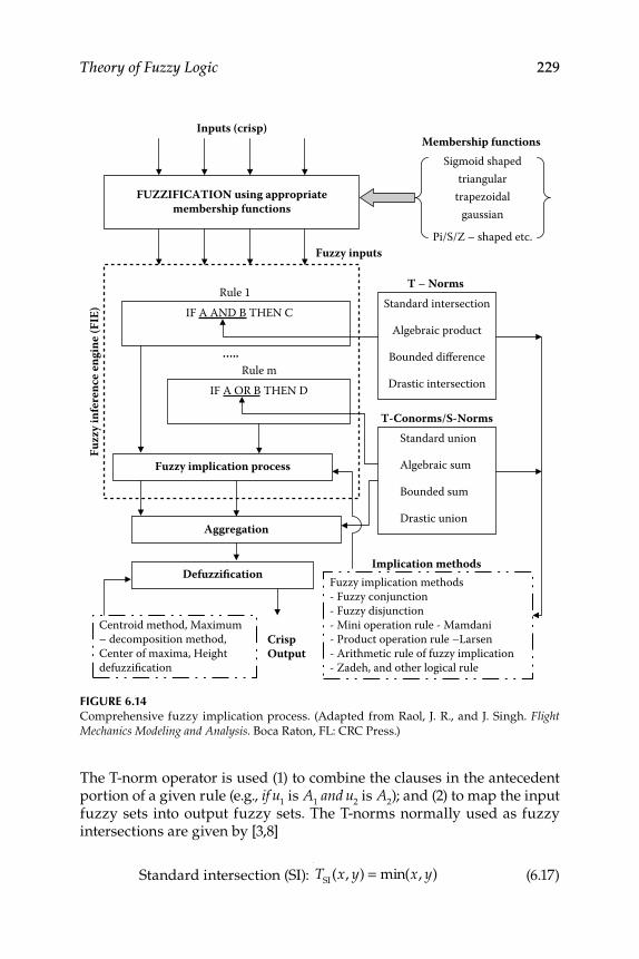
Theory of Fuzzy Logic 229

The T-norm operator is used (1) to combine the clauses in the antecedent portion of a given rule (e.g., if u1 is A1 and u2 is A2); and (2) to map the input fuzzy sets into output fuzzy sets. The T-norms normally used as fuzzy intersections are given by [3,8]

Standard intersection (SI): TSI

(x, y) = min(x, y) (6.17)

FIGURE 6.14Comprehensive fuzzy implication process. (Adapted from Raol, J. R., and J. Singh. Flight Mechanics Modeling and Analysis. Boca Raton, FL: CRC Press.)

Inputs (crisp)

Sigmoid shapedtriangular

trapezoidalgaussian

Pi/S/Z – shaped etc. Fuzzy inputs

CrispOutput

FUZZIFICATION using appropriatemembership functions

Membership functions

Rule 1

…..Rule m

Standard intersection

Algebraic product

Bounded difference

Drastic intersection

T – Norms

Standard union

Algebraic sum

Bounded sum

Drastic union

T-Conorms/S-Norms

IF A AND B THEN C

IF A OR B THEN D

Fuzzy implication process

Fuzzy implication methods- Fuzzy conjunction- Fuzzy disjunction- Mini operation rule - Mamdani- Product operation rule –Larsen- Arithmetic rule of fuzzy implication- Zadeh, and other logical rule

Implication methods

Aggregation

Defuzzification

Centroid method, Maximum– decomposition method,Center of maxima, Heightdefuzzification

Fuzz

y in

fere

nce

engi

ne (F

IE)

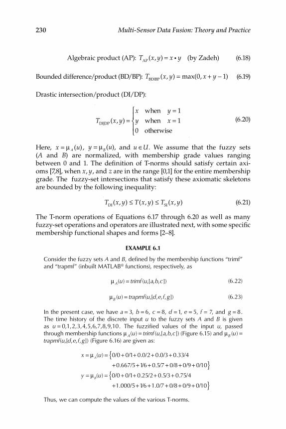
230 Multi-Sensor Data Fusion: Theory and Practice

Algebraic product (AP): TAP

(x, y) = x g y (by Zadeh) (6.18)

Bounded difference/product (BD/BP): TBD|BP(x, y) = max(0, x + y − 1) (6.19)

Drastic intersection/product (DI/DP):

TDI|DP

(x, y) =x when y = 1

y when x = 1

0 otherwise

⎧

⎨⎪

⎩⎪

(6.20)

Here, x = μA (u), y = μB(u), and u ∈U. We assume that the fuzzy sets (A and B) are normalized, with membership grade values ranging between 0 and 1. The defi nition of T-norms should satisfy certain axi-oms [7,8], when x, y, and z are in the range [0,1] for the entire membership grade. The fuzzy-set intersections that satisfy these axiomatic skeletons are bounded by the following inequality:

TDI

(x, y) ≤ T(x, y) ≤ TSI

(x, y) (6.21)

The T-norm operations of Equations 6.17 through 6.20 as well as many fuzzy-set operations and operators are illustrated next, with some specifi c membership functional shapes and forms [2–8].

EXAMPLE 6.1

Consider the fuzzy sets A and B, defi ned by the membership functions “trimf” and “trapmf” (inbuilt MATLAB® functions), respectively, as

μA(u) = trimf (u,[a,b,c]) (6.22)

μB (u) = trapmf(u,[d,e,f,g]) (6.23)

In the present case, we have a = 3, b = 6, c = 8, d = 1, e = 5, f = 7, and g = 8 . The time history of the discrete input u to the fuzzy sets A and B is given as u = 0,1,2,3,4,5,6,7,8,9,10. The fuzzifi ed values of the input u, passed through membership functions μA(u) = trimf (u,[a,b,c]) (Figure 6.15) and μB (u) = trapmf(u,[d,e,f,g]) (Figure 6.16) are given as:

x = μA(u) = 0/0 + 0/1+ 0.0/2+ 0.0/3+ 0.33/4{+0.667/5+1/6 + 0.5/7 + 0/8 + 0/9 + 0/10}

y = μB(u) = 0/0 + 0/1+ 0.25/2+ 0.5/3+ 0.75/4{+1.000/5+1/6 +1.0/7 + 0/8 + 0/9 + 0/10}

Thus, we can compute the values of the various T-norms.

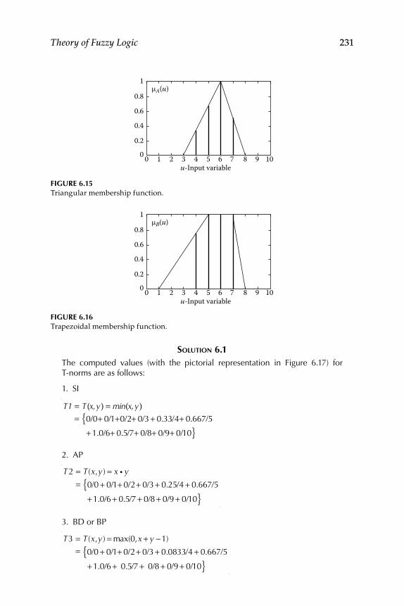
Theory of Fuzzy Logic 231

SOLUTION 6.1The computed values (with the pictorial representation in Figure 6.17) for T-norms are as follows:

1. SI

T1 = T(x,y) = min(x,y)

= 0/0+ 0/1 +0/2+ 0/3 + 0.33/4+ 0.667/5{ + 1.0/6+ 0.5/7+ 0/8+ 0/9+ 0/10}

2. AP

T2 = T(x,y) = x g y

= 0/0 + 0/1 + 0/2+ 0/3 + 0.25/4 + 0.667/5{ + 1.0/6 + 0.5/7 + 0/8 + 0/9 + 0/10}

3. BD or BP

T3 = T(x,y) = max(0,x + y −1)= 0/0 + 0/1 + 0/2+ 0/3 + 0.0833/4 + 0.667/5{

+ 1.0/6 + 0.5/7 + 0/8 + 0/9 + 0/10}

FIGURE 6.15Triangular membership function.

mA(u)

u-Input variable

1

0.8

0.6

0.4

0.2

0 0 1 2 3 4 5 6 7 8 9 10

FIGURE 6.16Trapezoidal membership function.

mB(u)

u-Input variable

1

0.8

0.6

0.4

0.2

0 0 1 2 3 4 5 6 7 8 9 10

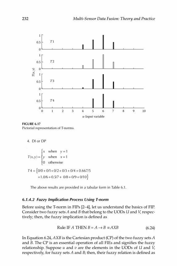
232 Multi-Sensor Data Fusion: Theory and Practice

4. DI or DP

T(x,y) =

x when y =1

y when x =1

0 otherwise

⎧

⎨⎪

⎩⎪

T4 = 0/0 + 0/1 +0/2+ 0/3 + 0/4 + 0.667/5{

+1.0/6+0.5/7+ 0/8+ 0/9+ 0/10}

The above results are provided in a tabular form in Table 6.1.

6.1.4.2 Fuzzy Implication Process Using T-norm

Before using the T-norm in FIPs [2–4], let us understand the basics of FIP. Consider two fuzzy sets A and B that belong to the UODs U and V, respec-tively; then, the fuzzy implication is defi ned as

Rule: IF A THEN B = A → B ≡ AXB (6.24)

In Equation 6.24, AXB is the Cartesian product (CP) of the two fuzzy sets A and B. The CP is an essential operation of all FIEs and signifi es the fuzzy relationship. Suppose u and v are the elements in the UODs of U and V, respectively, for fuzzy sets A and B; then, their fuzzy relation is defi ned as

FIGURE 6.17Pictorial representation of T-norms.

T 1

T 2

T 3

T(x,

y)

T 4

1

0.5

01

0.5

01

0.5

01

0.5

0

u-Input variable0 1 2 3 4 5 6 7 8 9 10

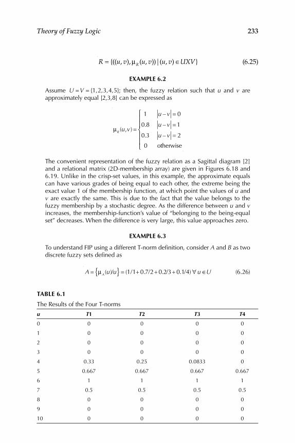
Theory of Fuzzy Logic 233

R = {((u, v), μR (u, v))|(u, v) ∈UXV} (6.25)

EXAMPLE 6.2

Assume U =V = {1,2,3,4,5}; then, the fuzzy relation such that u and v are approximately equal [2,3,8] can be expressed as

μR (u,v) =

1 u – v = 0

0.8 u – v =1

0.3 u – v = 2

0 otherwise

⎧

⎨

⎪⎪

⎩

⎪⎪

The convenient representation of the fuzzy relation as a Sagittal diagram [2] and a relational matrix (2D-membership array) are given in Figures 6.18 and 6.19. Unlike in the crisp-set values, in this example, the approximate equals can have various grades of being equal to each other, the extreme being the exact value 1 of the membership function, at which point the values of u and v are exactly the same. This is due to the fact that the value belongs to the fuzzy membership by a stochastic degree. As the difference between u and v increases, the membership-function’s value of “belonging to the being-equal set” decreases. When the difference is very large, this value approaches zero.

EXAMPLE 6.3

To understand FIP using a different T-norm defi nition, consider A and B as two discrete fuzzy sets defi ned as

A = μA(u)/u{ } = (1/1+0.7/2+0.2/3+0.1/4) ∀ u ∈U (6.26)

TABLE 6.1

The Results of the Four T-norms

u T1 T2 T3 T4

0 0 0 0 0

1 0 0 0 0

2 0 0 0 0

3 0 0 0 0

4 0.33 0.25 0.0833 0

5 0.667 0.667 0.667 0.667

6 1 1 1 1

7 0.5 0.5 0.5 0.5

8 0 0 0 0

9 0 0 0 0

10 0 0 0 0

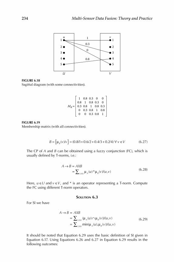
234 Multi-Sensor Data Fusion: Theory and Practice

B = μB (v)/v{ } = (0.8/1+0.6/2+0.4/3+0.2/4) ∀ v ∈V (6.27)

The CP of A and B can be obtained using a fuzzy conjunction (FC), which is usually defi ned by T-norms, i.e.:

A → B = AXB

= μAUXV∑ (u) *μB (v)/(u,v) (6.28)

Here, u ∈U and v ∈V , and * is an operator representing a T-norm. Compute the FC using different T-norm operators.

SOLUTION 6.3For SI we have

A → B = AXB

= (μA (u)∩ μB (v))/(u,v)UXV∑

= min(μA (u),μB (v))/(u,v)UXV∑

(6.29)

It should be noted that Equation 6.29 uses the basic defi nition of SI given in Equation 6.17. Using Equations 6.26 and 6.27 in Equation 6.29 results in the following outcomes:

FIGURE 6.18Sagittal diagram (with some connectivities).

U V

1

2345

1

2345

1

0

0.3

0.8

u v

FIGURE 6.19Membership matrix (with all connectivities).

00

0.30.81

00.30.81

0.8

0.30.81

0.80.3

0.81

0.80.30

10.80.300

MR =

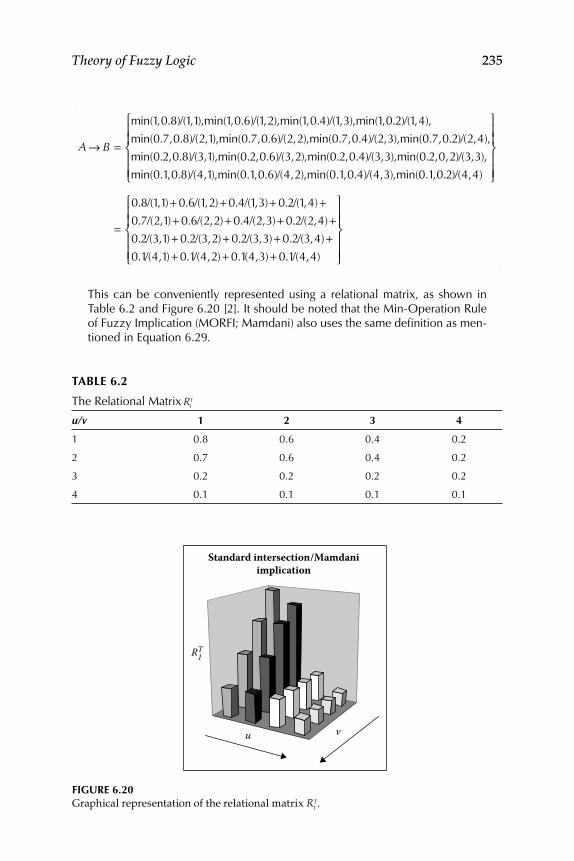
Theory of Fuzzy Logic 235

A → B =

min(1,0.8)/(1,1),min(1,0.6)/(1,2),min(1,0.4)/(1,3),min(1,0.2)/(1,4),

min(0.7,0.8)/(2,1),min(0.7,0.6)/(2,2),min(0.7,0.4)/(2,3),min(0.7,0.2)/(2,4),

min(0.2,0.8)/(3,1),min(0.2,0.6)/(3,2),min(0.2,0.4)/(3,3),min(0.2,0,2)/(3,3),

min(0.1,0.8)/(4,1),min(0.1,0.6)/(4,2),min(0.1,0.4)/(4,3),min(0.1,0.2)/(4,4)

⎧

⎨⎪⎪

⎩⎪⎪

⎫

⎬⎪⎪

⎭⎪⎪

=

0.8/(1,1) + 0.6/(1,2) + 0.4/(1,3)+ 0.2/(1,4)+0.7/(2,1) + 0.6/(2,2) + 0.4/(2,3)+ 0.2/(2,4)+0.2/(3,1) + 0.2/(3,2) + 0.2/(3,3)+ 0.2/(3,4)+0.1/(4,1) + 0.1/(4,2) + 0.1(4,3) + 0.1/(4,4)

⎧

⎨⎪⎪

⎩⎪⎪

⎫

⎬⎪⎪

⎭⎪⎪

This can be conveniently represented using a relational matrix, as shown in Table 6.2 and Figure 6.20 [2]. It should be noted that the Min-Operation Rule of Fuzzy Implication (MORFI; Mamdani) also uses the same defi nition as men-tioned in Equation 6.29.

TABLE 6.2

The Relational Matrix R1T

u/v 1 2 3 4

1 0.8 0.6 0.4 0.2

2 0.7 0.6 0.4 0.2

3 0.2 0.2 0.2 0.2

4 0.1 0.1 0.1 0.1

FIGURE 6.20Graphical representation of the relational matrix R

1T.

Standard intersection/Mamdaniimplication

u v

RT1

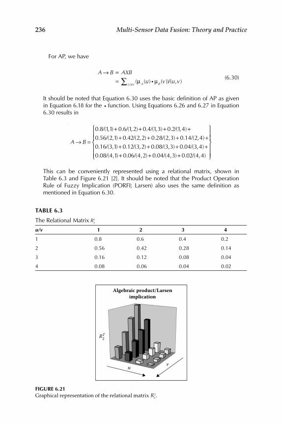
236 Multi-Sensor Data Fusion: Theory and Practice

For AP, we have

A → B = AXB

= (μA (u) g μB (v))/(u,v)UXV∑ (6.30)

It should be noted that Equation 6.30 uses the basic defi nition of AP as given in Equation 6.18 for the g function. Using Equations 6.26 and 6.27 in Equation 6.30 results in

A → B =

0.8/(1,1) + 0.6/(1,2) + 0.4/(1,3)+ 0.2/(1,4)+0.56/(2,1) + 0.42/(2,2) + 0.28/(2,3)+ 0.14/(2,4)+0.16/(3,1) + 0.12/(3,2) + 0.08/(3,3)+ 0.04/(3,4)+0.08/(4,1) + 0.06/(4,2) + 0.04/(4,3)+ 0.02/(4,4)

⎧

⎨⎪⎪

⎩⎪⎪

⎫

⎬⎪⎪

⎭⎪⎪

This can be conveniently represented using a relational matrix, shown in Table 6.3 and Figure 6.21 [2]. It should be noted that the Product Operation Rule of Fuzzy Implication (PORFI; Larsen) also uses the same defi nition as mentioned in Equation 6.30.

TABLE 6.3

The Relational Matrix R2T

u/v 1 2 3 4

1 0.8 0.6 0.4 0.2

2 0.56 0.42 0.28 0.14

3 0.16 0.12 0.08 0.04

4 0.08 0.06 0.04 0.02

FIGURE 6.21Graphical representation of the relational matrix R

2T.

Algebraic product/Larsenimplication

u v

RT2

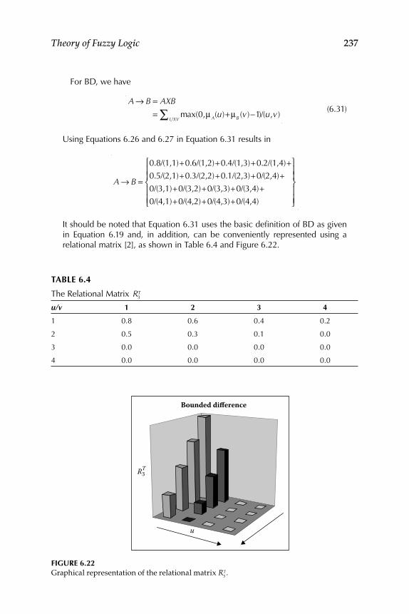
Theory of Fuzzy Logic 237

For BD, we have

A → B = AXB

= max(0,μA(u)+μB (v)−1)/(u,v)UXV∑

(6.31)

Using Equations 6.26 and 6.27 in Equation 6.31 results in

A → B =

0.8/(1,1)+0.6/(1,2)+0.4/(1,3)+0.2/(1,4)+

0.5/(2,1)+0.3/(2,2)+0.1/(2,3)+0/(2,4)+

0/(3,1)+0/(3,2)+0/(3,3)+0/(3,4)+

0/(4,1)+0/(4,2)+0/(4,3)+0/(4,4)

⎧

⎨⎪⎪

⎩⎪⎪

⎫

⎬⎪⎪

⎭⎪⎪

It should be noted that Equation 6.31 uses the basic defi nition of BD as given in Equation 6.19 and, in addition, can be conveniently represented using a relational matrix [2], as shown in Table 6.4 and Figure 6.22.

TABLE 6.4

The Relational Matrix R3T

u/v 1 2 3 4

1 0.8 0.6 0.4 0.2

2 0.5 0.3 0.1 0.0

3 0.0 0.0 0.0 0.0

4 0.0 0.0 0.0 0.0

FIGURE 6.22Graphical representation of the relational matrix R

3T.

Bounded difference

u

RT3

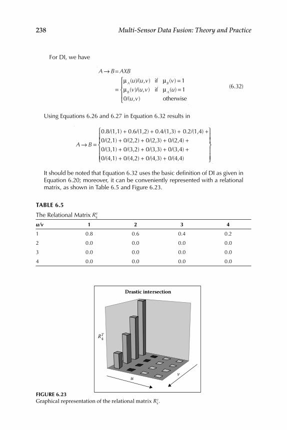
238 Multi-Sensor Data Fusion: Theory and Practice

For DI, we have

A → B= AXB

=μA (u)/(u,v) if μB (v) = 1

μB (v)/(u,v) if μA (u) = 1

0/(u,v) otherwise

⎧

⎨⎪

⎩⎪

(6.32)

Using Equations 6.26 and 6.27 in Equation 6.32 results in

A → B =

0.8/(1,1) + 0.6/(1,2) + 0.4/(1,3) + 0.2/(1,4) +

0/(2,1) + 0/(2,2) + 0/(2,3) + 0/(2,4) +

0/(3,1) + 0/(3,2) + 0/(3,3) + 0/(3,4) +

0/(4,1) + 0/(4,2) + 0/(4,3) + 0/(4,4)

⎧

⎨⎪⎪

⎩⎪⎪

⎫

⎬⎪⎪

⎭⎪⎪

It should be noted that Equation 6.32 uses the basic defi nition of DI as given in Equation 6.20; moreover, it can be conveniently represented with a relational matrix, as shown in Table 6.5 and Figure 6.23.

TABLE 6.5

The Relational Matrix R4T

u/v 1 2 3 4

1 0.8 0.6 0.4 0.2

2 0.0 0.0 0.0 0.0

3 0.0 0.0 0.0 0.0

4 0.0 0.0 0.0 0.0

FIGURE 6.23Graphical representation of the relational matrix R

4T.

Drastic intersection

uv

RT4

Theory of Fuzzy Logic 239

6.1.4.3 Triangular Conorm or S-norm

In FL, the operator corresponding to the operator or of Boolean logic is max (see Equation 6.12). The other possible or is defi ned by Equation 6.15. It is called a triangular conorm (T-conorm) or S-norm and is defi ned as follows: The union of two fuzzy sets A and B is specifi ed by a binary operation on the unit interval, i.e., a function of the form

S: [0,1]X[0,1] → [0,1]

or more specifi cally,

μA∪B(u) = S(μA(u),μB(u)) (6.33)

This fuzzy operator is used (1) to combine the clauses in the anteced-ent part of a given rule, such as “if u1 is A1 or u2 is A2” (see the S-norm block in Figure 6.14); and (2) in FIPs. The T-conorms used as fuzzy unions [3,8] are

Standard union (SU): SSU

(x, y) = max(x, y) (6.34)

Algebraic sum (AS): SAS(x, y) = x + y − x g y (Zadeh) (6.35)

Bounded sum (BS): S

BS(x, y) = min(1, x + y) (6.36)

Drastic union (DU):

SDU

(x, y) =x when y = 0

y when x = 0

1 otherwise

⎧

⎨⎪

⎩⎪

(6.37)

Disjoint sum: SDS

(x, y) = max{min(x, 1 − y), min(1 − x, y)} (6.38)

Here, x = μA(u) , y = μB(u) , and u ∈U. The fuzzy set unions that satisfy cer-tain axioms are bounded by the following inequality:

SSU

(x, y) ≤ S(x, y) ≤ SDU

(x, y) (6.39)

EXAMPLE 6.4

Consider Example 6.3. Compute the S-norms.

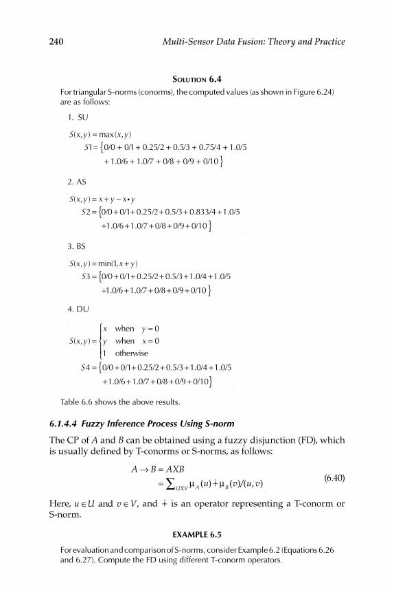
240 Multi-Sensor Data Fusion: Theory and Practice

SOLUTION 6.4For triangular S-norms (conorms), the computed values (as shown in Figure 6.24) are as follows:

1. SU

S(x,y) = max(x,y)

S1= 0/0 + 0/1+ 0.25/2 + 0.5/3 + 0.75/4 + 1.0/5{+ 1.0/6 + 1.0/7 + 0/8 + 0/9 + 0/10 }

2. AS

S(x,y) = x + y − xgy

S2 = 0/0 + 0/1+ 0.25/2+ 0.5/3+ 0.833/4 +1.0/5{+1.0/6 +1.0/7 + 0/8 + 0/9 + 0/10 }

3. BS

S(x,y) = min(1,x + y)

S3 = 0/0 + 0/1+ 0.25/2+ 0.5/3+1.0/4 +1.0/5{+1.0/6 +1.0/7 + 0/8 + 0/9 + 0/10 }

4. DU

S(x,y) =x when y = 0

y when x = 0

1 otherwise

⎧

⎨⎪

⎩⎪

S4 = 0/0 + 0/1+ 0.25/2+ 0.5/3+1.0/4 +1.0/5{+1.0/6 +1.0/7 + 0/8 + 0/9 + 0/10}

Table 6.6 shows the above results.

6.1.4.4 Fuzzy Inference Process Using S-norm

The CP of A and B can be obtained using a fuzzy disjunction (FD), which is usually defi ned by T-conorms or S-norms, as follows:

A → B = AXB

= μA (u) &+ μB(v)/(u, v)UXV∑ (6.40)

Here, u ∈U and v ∈V, and &+ is an operator representing a T-conorm or S-norm.

EXAMPLE 6.5

For evaluation and comparison of S-norms, consider Example 6.2 (Equations 6.26 and 6.27). Compute the FD using different T-conorm operators.

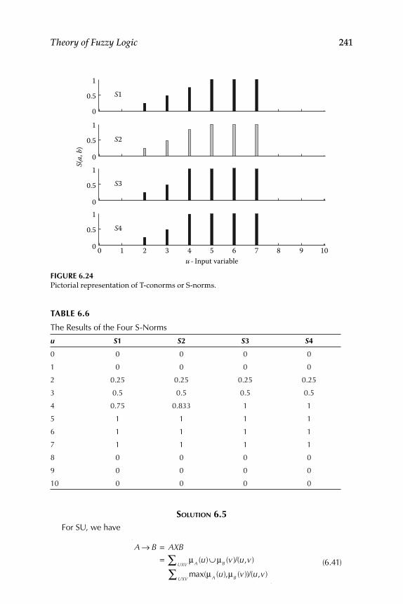
Theory of Fuzzy Logic 241

SOLUTION 6.5For SU, we have

A → B = AXB

= μA (u)∪ μB (v)/(u,v)UXV∑

max(μA (u),μB (v))/(u,v)UXV∑

(6.41)

FIGURE 6.24Pictorial representation of T-conorms or S-norms.

1

0.5 S1

S2

S3

S4

01

0.5

S(a,

b)

01

0.5

01

0.5

0 0 1 2 3 4 5u - Input variable

6 7 8 9 10

TABLE 6.6

The Results of the Four S-Norms

u S1 S2 S3 S4

0 0 0 0 0

1 0 0 0 0

2 0.25 0.25 0.25 0.25

3 0.5 0.5 0.5 0.5

4 0.75 0.833 1 1

5 1 1 1 1

6 1 1 1 1

7 1 1 1 1

8 0 0 0 0

9 0 0 0 0

10 0 0 0 0

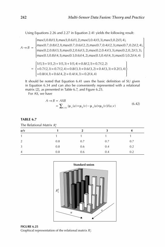
242 Multi-Sensor Data Fusion: Theory and Practice

Using Equations 2.26 and 2.27 in Equation 2.41 yields the following result:

A → B =

max(1,0.8)/(1,1),max(1,0.6)/(1,2),max(1,0.4)/(1,3),max(1,0.2)/(1,4),

max(0.7,0.8)/(2,1),max(0.7,0.6)/(2,2),max(0.7,0.4)/(2,3),max(0.7,0.2)/(2,4),

max(0.2,0.8)/(3,1),max(0.2,0.6)/(3,2),max(0.2,0.4)/(3,3),max(0.2,0,2)/(3,3),

max(0.1,0.8)/(4,1),max(0.1,0.6)/(4,2),max(0.1,0.4)/(4,3),max(0.1,0.2)/(4,4)

⎧

⎨⎪⎪

⎩⎪⎪

⎫

⎬⎪⎪

⎭⎪⎪

=1/(1,1)+1/(1,2) +1/(1,3) +1/(1,4)+0.8/(2,1) + 0.7/(2,2)

+0.7/(2,3)+ 0.7/(2,4) + 0.8/(3,1) + 0.6/(3,2) + 0.4/(3,3)+ 0.2/(3,4)

+0.8/(4,1) + 0.6/(4,2) + 0.4/(4,3) + 0.2/(4,4)

⎧

⎨⎪

⎩⎪

⎫

⎬⎪

⎭⎪

It should be noted that Equation 6.41 uses the basic defi nition of SU given in Equation 6.34 and can also be conveniently represented with a relational matrix [2], as presented in Table 6.7, and Figure 6.25.

For AS, we have

A → B = AXB

= (μA (u)+ μB (v) − μA (u)gμB (v))/(u,v)UXV∑ (6.42)

TABLE 6.7

The Relational Matrix R1S

u/v 1 2 3 4

1 1 1 1 1

2 0.8 0.7 0.7 0.7

3 0.8 0.6 0.4 0.2

4 0.8 0.6 0.4 0.2

FIGURE 6.25Graphical representation of the relational matrix R

1S.

Standard union

u v

RS1

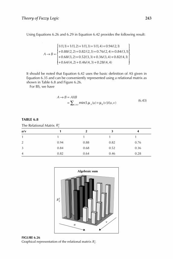
Theory of Fuzzy Logic 243

Using Equations 6.26 and 6.29 in Equation 6.42 provides the following result:

A → B =

1/(1,1) +1/(1,2)+1/(1,3)+1/(1,4) + 0.94/(2,1)

+0.88/(2,2) + 0.82/(2,3)+ 0.76/(2,4)+ 0.84/(3,1)

+0.68/(3,2) + 0.52/(3,3)+ 0.36/(3,4) + 0.82/(4,1)

+0.64/(4,2) + 0.46/(4,3) + 0.28/(4,4)

⎧

⎨⎪⎪

⎩⎪⎪

⎫

⎬⎪⎪

⎭⎪⎪

It should be noted that Equation 6.42 uses the basic defi nition of AS given in Equation 6.35 and can be conveniently represented using a relational matrix as shown in Table 6.8 and Figure 6.26.

For BS, we have

A → B = AXB

= min(1,μA (u)+ μB (v))/(u,v)UXV∑

(6.43)

TABLE 6.8

The Relational Matrix R2S

u/v 1 2 3 4

1 1 1 1 1

2 0.94 0.88 0.82 0.76

3 0.84 0.68 0.52 0.36

4 0.82 0.64 0.46 0.28

FIGURE 6.26Graphical representation of the relational matrix R

2S.

Algebraic sum

uv

RS2

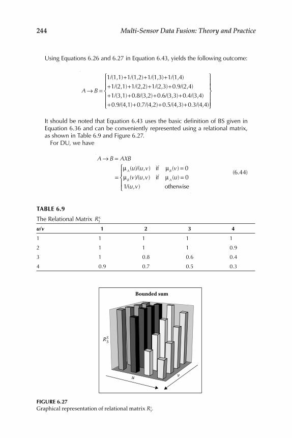
244 Multi-Sensor Data Fusion: Theory and Practice

Using Equations 6.26 and 6.27 in Equation 6.43, yields the following outcome:

A → B =

1/(1,1)+1/(1,2)+1/(1,3)+1/(1,4)

+1/(2,1)+1/(2,2)+1/(2,3)+0.9/(2,4)

+1/(3,1)+0.8/(3,2)+0.6/(3,3)+0.4/(3,4)

+0.9/(4,1)+0.7/(4,2)+0.5/(4,3)+0.3/(4,4)

⎧

⎨⎪⎪

⎩⎪⎪

⎫

⎬⎪⎪

⎭⎪⎪

It should be noted that Equation 6.43 uses the basic defi nition of BS given in Equation 6.36 and can be conveniently represented using a relational matrix, as shown in Table 6.9 and Figure 6.27.

For DU, we have

A → B = AXB

=μA (u)/(u,v) if μB (v) = 0

μB (v)/(u,v) if μA (u) = 0

1/(u,v) otherwise

⎧

⎨⎪

⎩⎪

(6.44)

TABLE 6.9

The Relational Matrix R3S

u/v 1 2 3 4

1 1 1 1 1

2 1 1 1 0.9

3 1 0.8 0.6 0.4

4 0.9 0.7 0.5 0.3

FIGURE 6.27Graphical representation of relational matrix R

3S.

Bounded sum

u v

RS3

Theory of Fuzzy Logic 245

Using Equations 6.26 and 6.27 in Equation 6.44 yields the following result:

A → B =

1/(1,1)+1/(1,2)+1/(1,3)+1/(1,4)

+1/(2,1)+1/(2,2)+1/(2,3)+1/(2,4)

+1/(3,1)+1/(3,2)+1/(3,3)+1/(3,4)

+1/(4,1)+1/(4,2)+1/(4,3)+1/(4,4)

⎧

⎨⎪⎪

⎩⎪⎪

⎫

⎬⎪⎪

⎭⎪⎪

It should be noted that Equation 6.44 uses the basic defi nition of DU given in Equation 6.37 and can be conveniently represented using a relational matrix as shown in Table 6.10 and Figure 6.28.

6.1.4.4.1 Fuzzy Complements

Consider a fuzzy set A with a membership grade of μA (u) for crisp input u in the UOD U. The standard defi nition of a fuzzy complement is given by

c(μA (u)) = μA (u) = 1 − μA (u) (6.45)

TABLE 6.10

Relational Matrix R4S

u/v 1 2 3 4

1 1 1 1 1

2 1 1 1 1

3 1 1 1 1

4 1 1 1 1

FIGURE 6.28Graphical representation of the relational matrix R

4S.

Drastic union

uv

RS4

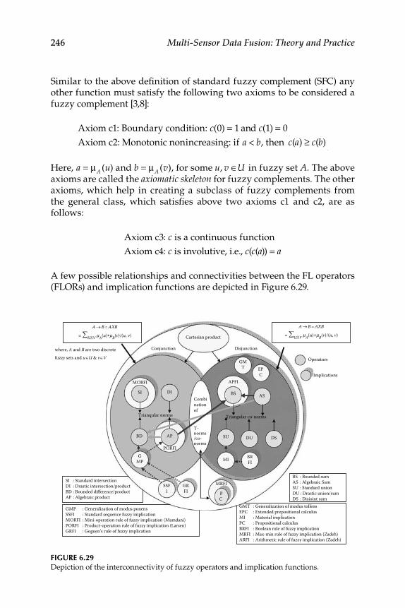
246 Multi-Sensor Data Fusion: Theory and Practice

Similar to the above defi nition of standard fuzzy complement (SFC) any other function must satisfy the following two axioms to be considered a fuzzy complement [3,8]:

Axiom c1: Boundary condition: c(0) = 1 and c(1) = 0

Axiom c2: Monotonic nonincreasing: if a < b, then c(a) ≥ c(b)

Here, a = μA (u) and b = μA (v), for some u, v ∈U in fuzzy set A. The above axioms are called the axiomatic skeleton for fuzzy complements. The other axioms, which help in creating a subclass of fuzzy complements from the general class, which satisfi es above two axioms c1 and c2, are as follows:

Axiom c3: c is a continuous function

Axiom c4: c is involutive, i.e., c(c(a)) = a

A few possible relationships and connectivities between the FL operators (FLORs) and implication functions are depicted in Figure 6.29.

FIGURE 6.29Depiction of the interconnectivity of fuzzy operators and implication functions.

A ® B = AXB

= åUXV μA(u)*μB(v)/(u, v)

A ® B = AXB

= åUXV μA(u)+μB(v)/(u, v)

where, A and B are two discretefuzzy sets and uÎU & vÎV

Conjunction

MORFI APFI

PORFI

Combinationof

T-norms/co-norms

GMP

SI : Standard intersectionDI : Drastic intersection/productBD : Bounded difference/productAP : Algebraic product

GMP : Generalization of modus ponensSSFI : Standard sequence fuzzy implicationMORFI : Mini-operation rule of fuzzy implication (Mamdani)PORFI : Product-operation rule of fuzzy implication (Larsen)GRFI : Goguen’s rule of fuzzy implication

GMT : Generalization of modus tollensEPC : Extended prepositional calculusMI : Material implicationPC : Propositional calculusBRFI : Boolean rule of fuzzy implicationMRFI : Max-min rule of fuzzy implication (Zadeh)ARFI : Arithmetic rule of fuzzy implication (Zadeh)

BS : Bounded sumAS : Algebraic SumSU : Standard unionDU : Drastic union/sumDS : Disioint sum

Trianqular norms

SI

GMT

Operators

ImplicationsEPC

BD

SSF1

GRFI

MRFI

PC

DI BS

SU DU DS

MI BRFI

AS

AP

Disjunction

Triangular co-norms

Cartesian product

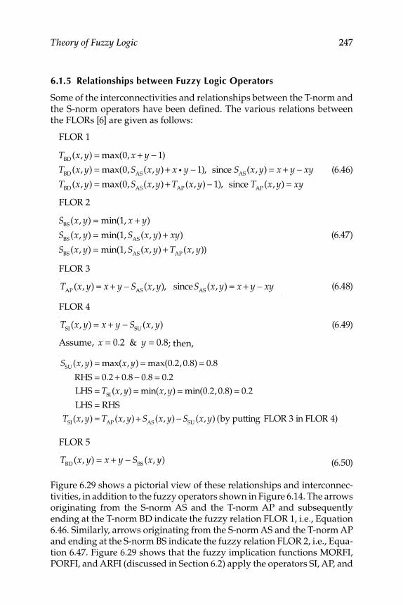
Theory of Fuzzy Logic 247

6.1.5 Relationships between Fuzzy Logic Operators

Some of the interconnectivities and relationships between the T-norm and the S-norm operators have been defi ned. The various relations between the FLORs [6] are given as follows:

FLOR 1

TBD

(x, y) = max(0, x + y − 1)

TBD

(x, y) = max(0,SAS

(x, y) + x g y − 1), since SAS

(x, y) = x + y − xy

TBD

(x, y) = max(0,SAS

(x, y) + TAP

(x, y) − 1), since TAP

(x, y) = xy

(6.46)

FLOR 2

SBS

(x, y) = min(1, x + y)

SBS

(x, y) = min(1, SAS

(x, y) + xy)

SBS

(x, y) = min(1, SAS

(x, y) + TAP

(x, y)) (6.47)

FLOR 3

T

AP(x, y) = x + y − S

AS(x, y), sinceS

AS(x, y) = x + y − xy (6.48)

FLOR 4

TSI

(x, y) = x + y − SSU

(x, y) (6.49)

Assume, x = 0.2 & y = 0.8; then,

SSU

(x, y) = max(x, y) = max(0.2, 0.8) = 0.8

RHS = 0.2 + 0.8 − 0.8 = 0.2

LHS = TSI

(x, y) = min(x, y) = min(0.2, 0.8) = 0.2

LHS = RHS

TSI

(x, y) = TAP

(x, y) + SAS

(x, y) − SSU

(x, y) (by putting FLOR 3 in FLOR 4)

FLOR 5

T

BD(x, y) = x + y − S

BS(x, y) (6.50)

Figure 6.29 shows a pictorial view of these relationships and interconnec-tivities, in addition to the fuzzy operators shown in Figure 6.14. The arrows originating from the S-norm AS and the T-norm AP and subsequently ending at the T-norm BD indicate the fuzzy relation FLOR 1, i.e., Equation 6.46. Similarly, arrows originating from the S-norm AS and the T-norm AP and ending at the S-norm BS indicate the fuzzy relation FLOR 2, i.e., Equa-tion 6.47. Figure 6.29 shows that the fuzzy implication functions MORFI, PORFI, and ARFI (discussed in Section 6.2) apply the operators SI, AP, and

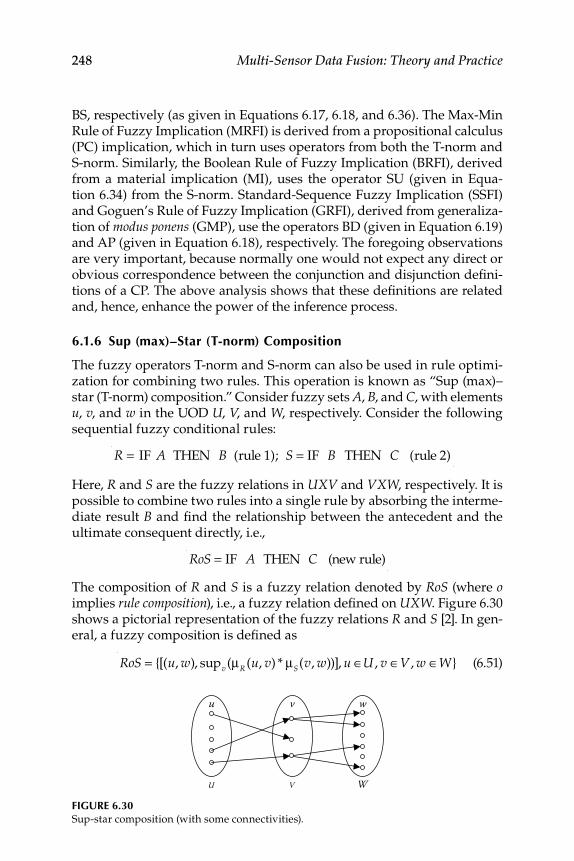
248 Multi-Sensor Data Fusion: Theory and Practice

BS, respectively (as given in Equations 6.17, 6.18, and 6.36). The Max-Min Rule of Fuzzy Implication (MRFI) is derived from a propositional calculus (PC) implication, which in turn uses operators from both the T-norm and S-norm. Similarly, the Boolean Rule of Fuzzy Implication (BRFI), derived from a material implication (MI), uses the operator SU (given in Equa-tion 6.34) from the S-norm. Standard-Sequence Fuzzy Implication (SSFI) and Goguen’s Rule of Fuzzy Implication (GRFI), derived from generaliza-tion of modus ponens (GMP), use the operators BD (given in Equation 6.19) and AP (given in Equation 6.18), respectively. The foregoing observations are very important, because normally one would not expect any direct or obvious correspondence between the conjunction and disjunction defi ni-tions of a CP. The above analysis shows that these defi nitions are related and, hence, enhance the power of the inference process.

6.1.6 Sup (max)–Star (T-norm) Composition

The fuzzy operators T-norm and S-norm can also be used in rule optimi-zation for combining two rules. This operation is known as “Sup (max)–star (T-norm) composition.” Consider fuzzy sets A, B, and C, with elements u, v, and w in the UOD U, V, and W, respectively. Consider the following sequential fuzzy conditional rules:

R = IF A THEN B (rule 1); S = IF B THEN C (rule 2)

Here, R and S are the fuzzy relations in UXV and VXW, respectively. It is possible to combine two rules into a single rule by absorbing the interme-diate result B and fi nd the relationship between the antecedent and the ultimate consequent directly, i.e.,

RoS = IF A THEN C (new rule)

The composition of R and S is a fuzzy relation denoted by RoS (where o implies rule composition), i.e., a fuzzy relation defi ned on UXW. Figure 6.30 shows a pictorial representation of the fuzzy relations R and S [2]. In gen-eral, a fuzzy composition is defi ned as

RoS = {[(u, w), supv (μR (u, v) * μS(v, w))], u ∈U , v ∈V , w ∈W} (6.51)

FIGURE 6.30Sup-star composition (with some connectivities).

U V W

u v w

Theory of Fuzzy Logic 249

Here, “sup” means supremum and is denoted as ∪, i.e., union or max (SU); and * represents the T-norms of either (1) SI, (2) AP, (3) BD, or (4) DI. There are different methods to compute the composition of fuzzy relations.

6.1.6.1 Maximum–Minimum Composition (Mamdani)

Max–min composition is defi ned as follows:

μRoS(u, w) = maxv min(μR (u, v), μS(v, w))

= ∪v (μR (u, v) ∩ μS(v, w)) (6.52)

If fuzzy relations R and S are given by relational matrices [2] (Tables 6.11 and 6.12), then

After completing the operations for all rows of R with all columns of S, RoS can be represented as shown in Table 6.13 (based on the relational matrices for R and S). It should be noted that in Equation 6.52 (for min), the basic defi nition of SI is used, i.e., Equation 6.17.

0.1 0.2 0.0 1.0 (R: fi rst row all columns)

0.9 0.2 0.8 0.4 (S: fi rst column all rows)

min 0.1 0.2 0.0 0.4 (μR(u, v) ∩ μS (v, w))

max 0.4 (∪v)

TABLE 6.12

Relational Matrix S

S α β γ

a 0.9 0.0 0.3

b 0.2 1.0 0.8

c 0.8 0.0 0.7

d 0.4 0.2 0.3

TABLE 6.11

Relational Matrix R

R a b c d

1 0.1 0.2 0.0 1.0

2 0.3 0.3 0.0 0.2

3 0.8 0.9 1.0 0.4

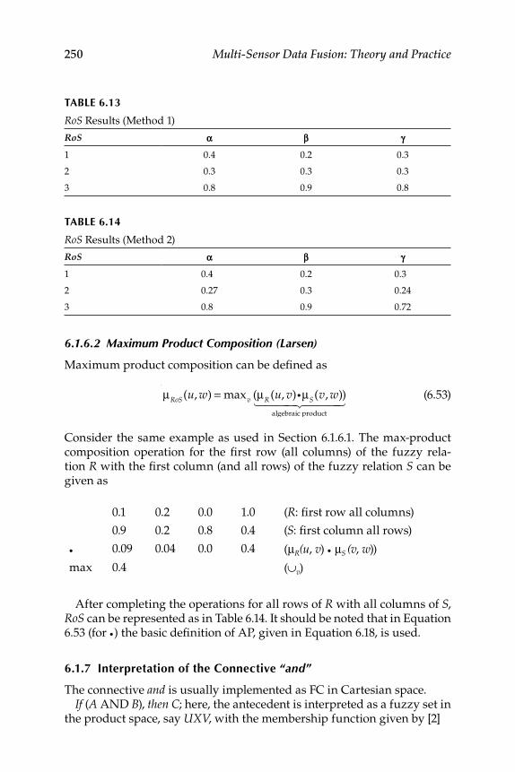
250 Multi-Sensor Data Fusion: Theory and Practice

6.1.6.2 Maximum Product Composition (Larsen)

Maximum product composition can be defi ned as

μRoS(u, w) = maxv (μR (u, v)gμS(v, w))

algebraic product

1 2444 3444

(6.53)

Consider the same example as used in Section 6.1.6.1. The max- product composition operation for the fi rst row (all columns) of the fuzzy rela-tion R with the fi rst column (and all rows) of the fuzzy relation S can be given as

After completing the operations for all rows of R with all columns of S, RoS can be represented as in Table 6.14. It should be noted that in Equation 6.53 (for g) the basic defi nition of AP, given in Equation 6.18, is used.

6.1.7 Interpretation of the Connective “and”

The connective and is usually implemented as FC in Cartesian space.If (A AND B), then C; here, the antecedent is interpreted as a fuzzy set in

the product space, say UXV, with the membership function given by [2]

0.1 0.2 0.0 1.0 (R: fi rst row all columns)

0.9 0.2 0.8 0.4 (S: fi rst column all rows)

g 0.09 0.04 0.0 0.4 (μR(u, v) g μS (v, w))

max 0.4 (∪v)

TABLE 6.14

RoS Results (Method 2)

RoS α β γ

1 0.4 0.2 0.3

2 0.27 0.3 0.24

3 0.8 0.9 0.72

TABLE 6.13

RoS Results (Method 1)

RoS α β γ

1 0.4 0.2 0.3

2 0.3 0.3 0.3

3 0.8 0.9 0.8

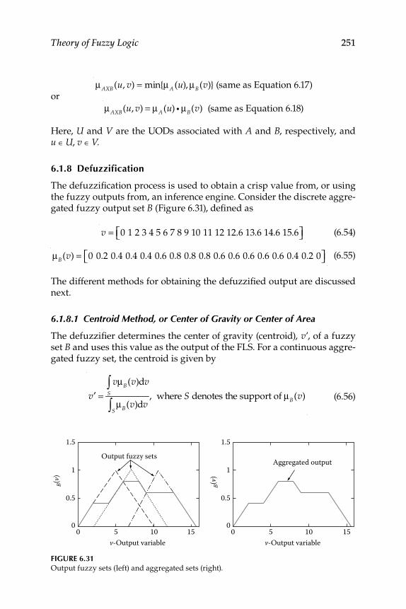
Theory of Fuzzy Logic 251

μAXB(u, v) = min{μA (u), μB(v)} (same as Equation 6.17)or

μAXB(u, v) = μA(u) g μB(v) (same as Equation 6.18)

Here, U and V are the UODs associated with A and B, respectively, and u ∈ U, v ∈ V.

6.1.8 Defuzzification

The defuzzifi cation process is used to obtain a crisp value from, or using the fuzzy outputs from, an inference engine. Consider the discrete aggre-gated fuzzy output set B (Figure 6.31), defi ned as

v = 0 1 2 3 4 5 6 7 8 9 10 11 12 12.6 13.6 14.6 15.6⎡⎣ ⎤⎦ (6.54)

μB(v) = 0 0.2 0.4 0.4 0.4 0.6 0.8 0.8 0.8 0.6 0.6 0.6 0.6 0.6 0.4 0.2 0⎡⎣ ⎤⎦

(6.55)

The different methods for obtaining the defuzzifi ed output are discussed next.

6.1.8.1 Centroid Method, or Center of Gravity or Center of Area

The defuzzifi er determines the center of gravity (centroid), v′, of a fuzzy set B and uses this value as the output of the FLS. For a continuous aggre-gated fuzzy set, the centroid is given by

v′ =vμB(v)dv

S∫

μB(v)dvS∫

, where S denotes the support of μB(v) (6.56)

FIGURE 6.31Output fuzzy sets (left) and aggregated sets (right).

v-Output variable

µ B(v

)

µ B(v

)

v-Output variable

1.5

Output fuzzy setsAggregated output

1

0.5

0

1.5

1

0.5

00 5 10 15 0 5 10 15

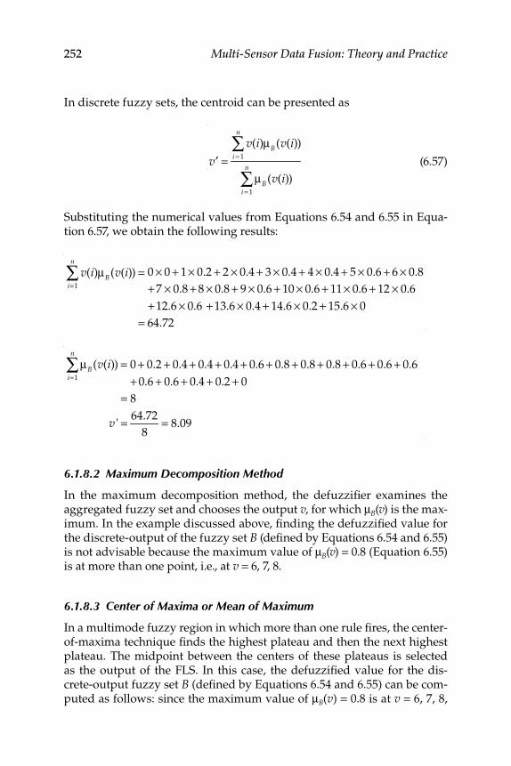
252 Multi-Sensor Data Fusion: Theory and Practice

In discrete fuzzy sets, the centroid can be presented as

v′ =v(i)μB(v(i))

i = 1

n

∑

μB(v(i))i = 1

n

∑ (6.57)

Substituting the numerical values from Equations 6.54 and 6.55 in Equa-tion 6.57, we obtain the following results:

v(i)μB(v(i))i=1

n

∑ = 0 × 0 + 1× 0.2 + 2 × 0.4 + 3 × 0.4 + 4 × 0.4 + 5 × 0.6 + 6 × 0.8

+ 7 × 0.8 + 8 × 0.8 + 9 × 0.6 + 10 × 0.6 + 11× 0.6 + 12 × 0.6

+ 12.6 × 0.6 + 13.6 × 0.4 + 14.6 × 0.2 + 15.6 × 0

= 64.72

μB(v(i)) = 0 + 0.2 + 0.4 + 0.4 + 0.4 + 0.6 + 0.8 + 0.8 + 0.8 + 0.6 + 0.6 + 0.6 i=1

n

∑+ 0.6 + 0.6 + 0.4 + 0.2 + 0

= 8

v ' = 64.72

8= 8.09

6.1.8.2 Maximum Decomposition Method

In the maximum decomposition method, the defuzzifi er examines the aggregated fuzzy set and chooses the output v, for which μB(v) is the max-imum. In the example discussed above, fi nding the defuzzifi ed value for the discrete-output of the fuzzy set B (defi ned by Equations 6.54 and 6.55) is not advisable because the maximum value of μB(v) = 0.8 (Equation 6.55) is at more than one point, i.e., at v = 6, 7, 8.

6.1.8.3 Center of Maxima or Mean of Maximum

In a multimode fuzzy region in which more than one rule fi res, the center-of-maxima technique fi nds the highest plateau and then the next highest plateau. The midpoint between the centers of these plateaus is selected as the output of the FLS. In this case, the defuzzifi ed value for the dis-crete-output fuzzy set B (defi ned by Equations 6.54 and 6.55) can be com-puted as follows: since the maximum value of μB(v) = 0.8 is at v = 6, 7, 8,

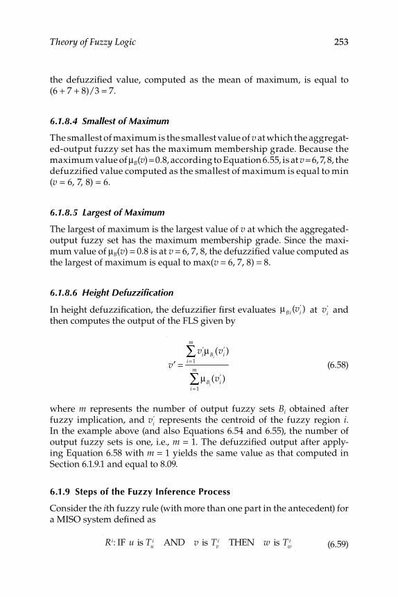
Theory of Fuzzy Logic 253

the defuzzifi ed value, computed as the mean of maximum, is equal to (6 + 7 + 8)/3 = 7.

6.1.8.4 Smallest of Maximum

The smallest of maximum is the smallest value of v at which the aggregat-ed-output fuzzy set has the maximum membership grade. Because the maximum value of μB(v) = 0.8, according to Equation 6.55, is at v = 6, 7, 8, the defuzzifi ed value computed as the smallest of maximum is equal to min(v = 6, 7, 8) = 6.

6.1.8.5 Largest of Maximum

The largest of maximum is the largest value of v at which the aggregated-output fuzzy set has the maximum membership grade. Since the maxi-mum value of μB(v) = 0.8 is at v = 6, 7, 8, the defuzzifi ed value computed as the largest of maximum is equal to max(v = 6, 7, 8) = 8.

6.1.8.6 Height Defuzzifi cation

In height defuzzifi cation, the defuzzifi er fi rst evaluates μBi (vi

′ ) at vi

′ and then computes the output of the FLS given by

v′ =vi

′μBi(vi

′ )i = 1

m

∑

μBi(vi

′ )i = 1

m

∑ (6.58)

where m represents the number of output fuzzy sets Bi obtained after fuzzy implication, and vi

′ represents the centroid of the fuzzy region i. In the example above (and also Equations 6.54 and 6.55), the number of output fuzzy sets is one, i.e., m = 1. The defuzzifi ed output after apply-ing Equation 6.58 with m = 1 yields the same value as that computed in Section 6.1.9.1 and equal to 8.09.

6.1.9 Steps of the Fuzzy Inference Process

Consider the ith fuzzy rule (with more than one part in the antecedent) for a MISO system defi ned as

Ri: IF u is Tu

i AND v is Tvi THEN w is Tw

i (6.59)

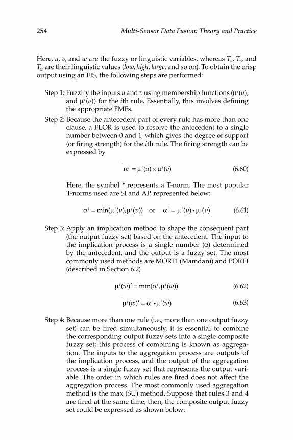
254 Multi-Sensor Data Fusion: Theory and Practice

Here, u, v, and w are the fuzzy or linguistic variables, whereas Tu, Tv, and Tw are their linguistic values (low, high, large, and so on). To obtain the crisp output using an FIS, the following steps are performed:

Step 1: Fuzzify the inputs u and v using membership functions (μ i (u), and μ i (v)) for the ith rule. Essentially, this involves defi ning the appropriate FMFs.

Step 2: Because the antecedent part of every rule has more than one clause, a FLOR is used to resolve the antecedent to a single number between 0 and 1, which gives the degree of support (or fi ring strength) for the ith rule. The fi ring strength can be expressed by

α i = μ i (u) × μ i (v) (6.60)

Here, the symbol * represents a T-norm. The most popular T-norms used are SI and AP, represented below:

αi = min(μ i(u),μ i(v)) or α i = μ i(u) g μ i(v) (6.61)

Step 3: Apply an implication method to shape the consequent part (the output fuzzy set) based on the antecedent. The input to the implication process is a single number (α) determined by the antecedent, and the output is a fuzzy set. The most commonly used methods are MORFI (Mamdani) and PORFI (described in Section 6.2)

μ i(w)′ = min(α i,μ i(w)) (6.62)

μ i(w)′ = α i gμ i(w) (6.63)

Step 4: Because more than one rule (i.e., more than one output fuzzy set) can be fi red simultaneously, it is essential to combine the corresponding output fuzzy sets into a single composite fuzzy set; this process of combining is known as aggrega-tion. The inputs to the aggregation process are outputs of the implication process, and the output of the aggregation process is a single fuzzy set that represents the output vari-able. The order in which rules are fi red does not affect the aggregation process. The most commonly used aggregation method is the max (SU) method. Suppose that rules 3 and 4 are fi red at the same time; then, the composite output fuzzy set could be expressed as shown below:

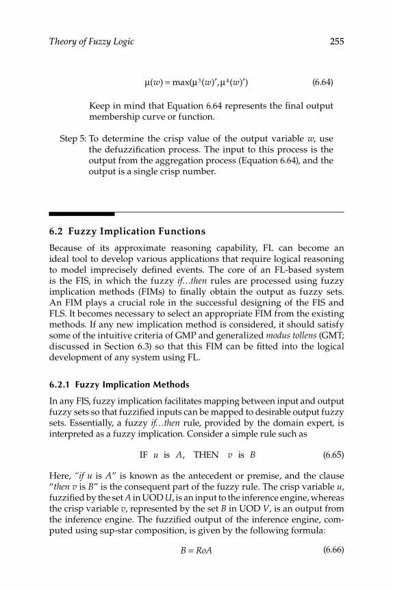
Theory of Fuzzy Logic 255

μ(w) = max(μ3(w)′,μ4(w)′) (6.64)

Keep in mind that Equation 6.64 represents the fi nal output membership curve or function.

Step 5: To determine the crisp value of the output variable w, use the defuzzifi cation process. The input to this process is the output from the aggregation process (Equation 6.64), and the output is a single crisp number.

6.2 Fuzzy Implication Functions

Because of its approximate reasoning capability, FL can become an ideal tool to develop various applications that require logical reasoning to model imprecisely defi ned events. The core of an FL-based system is the FIS, in which the fuzzy if…then rules are processed using fuzzy implication methods (FIMs) to fi nally obtain the output as fuzzy sets. An FIM plays a crucial role in the successful designing of the FIS and FLS. It becomes necessary to select an appropriate FIM from the existing methods. If any new implication method is considered, it should satisfy some of the intuitive criteria of GMP and generalized modus tollens (GMT; discussed in Section 6.3) so that this FIM can be fi tted into the logical development of any system using FL.

6.2.1 Fuzzy Implication Methods

In any FIS, fuzzy implication facilitates mapping between input and output fuzzy sets so that fuzzifi ed inputs can be mapped to desirable output fuzzy sets. Essentially, a fuzzy if…then rule, provided by the domain expert, is interpreted as a fuzzy implication. Consider a simple rule such as

IF u is A, THEN v is B (6.65)

Here, “if u is A” is known as the antecedent or premise, and the clause “then v is B” is the consequent part of the fuzzy rule. The crisp variable u, fuzzifi ed by the set A in UOD U, is an input to the inference engine, whereas the crisp variable v, represented by the set B in UOD V, is an output from the inference engine. The fuzzifi ed output of the inference engine, com-puted using sup-star composition, is given by the following formula:

B = RoA (6.66)

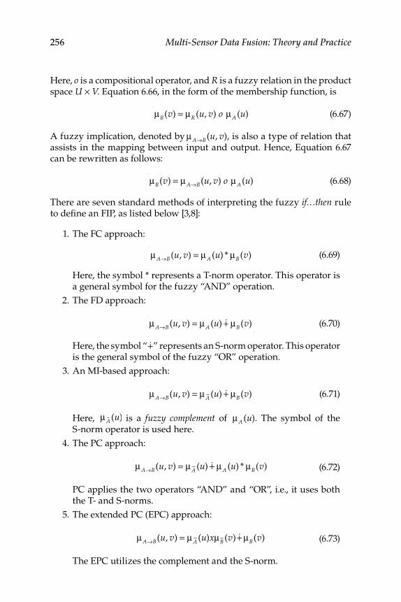
256 Multi-Sensor Data Fusion: Theory and Practice

Here, o is a compositional operator, and R is a fuzzy relation in the product space U × V. Equation 6.66, in the form of the membership function, is

μB(v) = μR (u, v) o μA (u) (6.67)

A fuzzy implication, denoted by μA→B(u, v), is also a type of relation that assists in the mapping between input and output. Hence, Equation 6.67 can be rewritten as follows:

μB(v) = μA→B(u, v) o μA (u) (6.68)

There are seven standard methods of interpreting the fuzzy if…then rule to defi ne an FIP, as listed below [3,8]:

1. The FC approach:

μA→B(u, v) = μA (u) * μB(v) (6.69)

Here, the symbol * represents a T-norm operator. This operator is a general symbol for the fuzzy “AND” operation.

2. The FD approach:

μA→B(u, v) = μA (u) &+ μB(v) (6.70)

Here, the symbol “ &+” represents an S-norm operator. This operator is the general symbol of the fuzzy “OR” operation.

3. An MI-based approach:

μA→B(u, v) = μA (u) &+ μB(v) (6.71)

Here, μA (u) is a fuzzy complement of μA (u). The symbol of the S-norm operator is used here.

4. The PC approach:

μA→B(u, v) = μA (u) &+ μA (u) * μB(v) (6.72)

PC applies the two operators “AND” and “OR”, i.e., it uses both the T- and S-norms.

5. The extended PC (EPC) approach:

μA→B(u, v) = μA (u)xμB (v) &+ μB(v) (6.73)

The EPC utilizes the complement and the S-norm.

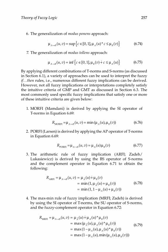
Theory of Fuzzy Logic 257

6. The generalization of modus ponens approach:

μA→B(u, v) = sup c ∈[0,1],μA (u) * c ≤ μB(v){ } (6.74)

7. The generalization of modus tollens approach:

μA→B(u, v) = inf c ∈[0, 1], μB(v) &+ c ≤ μA (u){ } (6.75)

By applying different combinations of T-norms and S-norms (as discussed in Section 6.1), a variety of approaches can be used to interpret the fuzzy if…then rules, i.e., numerous different fuzzy implications can be derived. However, not all fuzzy implications or interpretations completely satisfy the intuitive criteria of GMP and GMT as discussed in Section 6.3. The most commonly used specifi c fuzzy implications that satisfy one or more of these intuitive criteria are given below:

1. MORFI (Mamdani) is derived by applying the SI operator of T-norms in Equation 6.69:

R

MORFI= μA→B(u, v) = min(μA (u),μB(v)) (6.76)

2. PORFI (Larsen) is derived by applying the AP operator of T-norms in Equation 6.69:

RPORFI

= μA→B(u, v) = μA (u)μB(v) (6.77)

3. The arithmetic rule of fuzzy implication (ARFI; Zadeh/ Lukasiewicz) is derived by using the BS operator of S-norms and the complement operator in Equation 6.71 to obtain the following:

RARFI

= μA→B(u, v) = μA (u) &+ μB(v)

= min (1, μA (u) + μB(v))

= min (1, 1 − μA (u) + μB(v))

(6.78)

4. The max-min rule of fuzzy implication (MRFI; Zadeh) is derived by using the SI operator of T-norms, the SU operator of S-norms, and the fuzzy-complement operator in Equation 6.72:

RMRFI

= μA→B(u, v) = μA (u) &+ μA (u) * μB(v)

= max(μA (u),μA (u) * μB(v))

= max(1 − μA (u),μA (u) * μB(v))

= max(1 − μA (u), min(μA (u),μB(v)))

(6.79)

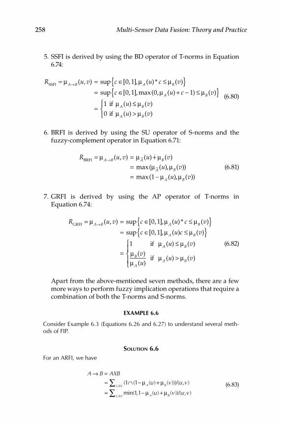
258 Multi-Sensor Data Fusion: Theory and Practice

5. SSFI is derived by using the BD operator of T-norms in Equation 6.74:

RSSFI

= μA→B(u, v) = sup c ∈[0,1],μA (u) * c ≤ μB(v){ }= sup c ∈[0,1], max(0,μA (u) + c − 1) ≤ μB(v){ }=

1 if μA (u) ≤ μB(v)

0 if μA (u) > μB(v)

⎧⎨⎩

(6.80)

6. BRFI is derived by using the SU operator of S-norms and the fuzzy-complement operator in Equation 6.71:

RBRFI

= μA→B(u, v) = μA (u) &+ μB(v)

= max(μA (u),μB(v))

= max(1 − μA (u),μB(v))

(6.81)

7. GRFI is derived by using the AP operator of T-norms in Equation 6.74:

RGRFI

= μA→B(u, v) = sup c ∈[0,1],μA (u) * c ≤ μB(v){ }= sup c ∈[0,1],μA (u)c ≤ μB(v){ }

=1 if μA (u) ≤ μB(v)

μB(v)

μA (u)if μA (u) > μB(v)

⎧⎨⎪

⎩⎪

(6.82)

Apart from the above-mentioned seven methods, there are a few more ways to perform fuzzy implication operations that require a combination of both the T-norms and S-norms.

EXAMPLE 6.6

Consider Example 6.3 (Equations 6.26 and 6.27) to understand several meth-ods of FIP.

SOLUTION 6.6For an ARFI, we have

A → B = AXB

= (1∩ (1− μA (u)+ μB (v)))/(u,v)UXV∑

= min(1,1− μA (u)+ μB (v))/(u,v)UXV∑

(6.83)

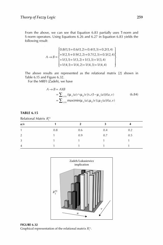
Theory of Fuzzy Logic 259

From the above, we can see that Equation 6.83 partially uses T-norm and S-norm operators. Using Equations 6.26 and 6.27 in Equation 6.83 yields the following result:

A → B =

0.8/(1,1) + 0.6/(1,2) + 0.4/(1,3)+ 0.2/(1,4)

+1/(2,1) + 0.9/(2,2) + 0.7/(2,3)+ 0.5/(2,4)

+1/(3,1)+1/(3,2)+1/(3,3)+1/(3,4)

+1/(4,1)+1/(4,2)+1/(4,3)+1/(4,4)

⎧

⎨⎪⎪

⎩⎪⎪

⎫

⎬⎪⎪

⎭⎪⎪

The above results are represented as the relational matrix [2] shown in Table 6.15 and Figure 6.32.

For the MRFI (Zadeh), we have

A → B = AXB

= ((μA (u)∩ μB (v))∪(1− μA (u)))/(u,v)UXV∑

= max(min(μA (u),μB (v)),μA (u))/(u,v)UXV∑

(6.84)

TABLE 6.15

Relational Matrix R1TS

u/v 1 2 3 4

1 0.8 0.6 0.4 0.2

2 1 0.9 0.7 0.5

3 1 1 1 1

4 1 1 1 1

Zadeh/Lukasiewiczimplication

uv

RTS1

FIGURE 6.32Graphical representation of the relational matrix R

1TS.

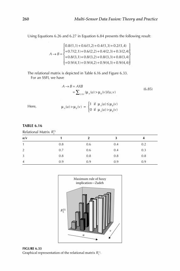
260 Multi-Sensor Data Fusion: Theory and Practice

Using Equations 6.26 and 6.27 in Equation 6.84 presents the following result:

A → B =

0.8/(1,1)+ 0.6/(1,2)+ 0.4/(1,3)+ 0.2/(1,4)

+0.7/(2,1)+ 0.6/(2,2)+ 0.4/(2,3)+ 0.3/(2,4)

+0.8/(3,1)+ 0.8/(3,2)+ 0.8/(3,3)+ 0.8/(3,4)

+0.9/(4,1)+ 0.9/(4,2)+ 0.9/(4,3)+ 0.9/(4,4)

⎧

⎨⎪⎪

⎩⎪⎪

⎫

⎬⎪⎪

⎭⎪⎪

The relational matrix is depicted in Table 6.16 and Figure 6.33.For an SSFI, we have

A → B = AXB

= (μA (u) > μB (v))/(u,v)UXV∑

(6.85)

Here,

μA (u) > μB (v) =1 if μA(u) ≤ μB(v)

0 if μA(u) > μB(v)

⎧⎨⎩

Maximum rule of fuzzyimplication—Zadeh

uv

R2TS

FIGURE 6.33Graphical representation of the relational matrix R

2TS.

TABLE 6.16

Relational Matrix R2TS

u/v 1 2 3 4

1 0.8 0.6 0.4 0.2

2 0.7 0.6 0.4 0.3

3 0.8 0.8 0.8 0.8

4 0.9 0.9 0.9 0.9

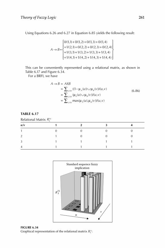
Theory of Fuzzy Logic 261

Using Equations 6.26 and 6.27 in Equation 6.85 yields the following result:

A → B=

0/(1,1)+ 0/(1,2)+ 0/(1,3)+ 0/(1,4)

+1/(2,1)+ 0/(2,2) + 0/(2,3)+ 0/(2,4)

+1/(3,1)+1/(3,2)+1/(3,3)+1/(3,4)

+1/(4,1)+1/(4,2)+1/(4,3)+1/(4,4)

⎧

⎨⎪⎪

⎩⎪⎪

⎫

⎬⎪⎪

⎭⎪⎪

This can be conveniently represented using a relational matrix, as shown in Table 6.17 and Figure 6.34.

For a BRFI, we have

A → B = AXB

= ((1− μA (u))∪ μB (v))/(u,v)UXV∑

= (μA (u)∪ μB (v))/(u,v)UXV∑

= max(μA (u),μB (v))/(u,v)UXV∑

(6.86)

Standard sequence fuzzyimplication

uv

RTS3

FIGURE 6.34Graphical representation of the relational matrix R

3TS.

TABLE 6.17

Relational Matrix R3TS

u/v 1 2 3 4

1 0 0 0 0

2 1 0 0 0

3 1 1 1 1

4 1 1 1 1

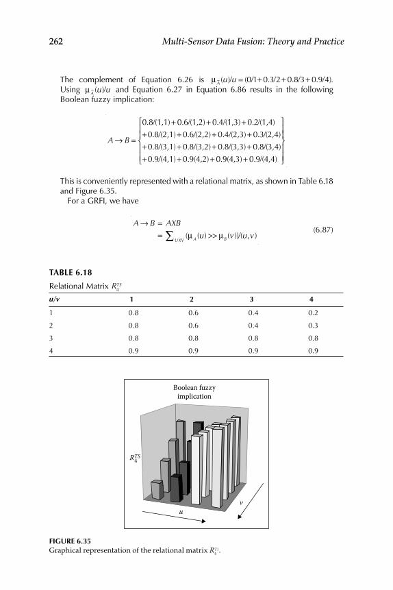
262 Multi-Sensor Data Fusion: Theory and Practice

The complement of Equation 6.26 is μA (u)/u = (0/1+ 0.3/2+ 0.8/3+ 0.9/4). Using μA (u)/u and Equation 6.27 in Equation 6.86 results in the following Boolean fuzzy implication:

A → B =

0.8/(1,1)+ 0.6/(1,2)+ 0.4/(1,3)+ 0.2/(1,4)

+0.8/(2,1)+ 0.6/(2,2)+ 0.4/(2,3)+ 0.3/(2,4)

+0.8/(3,1)+ 0.8/(3,2)+ 0.8/(3,3)+ 0.8/(3,4)

+0.9/(4,1)+ 0.9(4,2) + 0.9(4,3) + 0.9/(4,4)

⎧

⎨⎪⎪

⎩⎪⎪

⎫

⎬⎪⎪

⎭⎪⎪

This is conveniently represented with a relational matrix, as shown in Table 6.18 and Figure 6.35.

For a GRFI, we have

A → B = AXB

= (μA (u) >> μB (v))/(u,v)UXV∑

(6.87)

Boolean fuzzyimplication

uv

RTS4

FIGURE 6.35Graphical representation of the relational matrix R

4TS.

TABLE 6.18

Relational Matrix R4TS

u/v 1 2 3 4

1 0.8 0.6 0.4 0.2

2 0.8 0.6 0.4 0.3

3 0.8 0.8 0.8 0.8

4 0.9 0.9 0.9 0.9

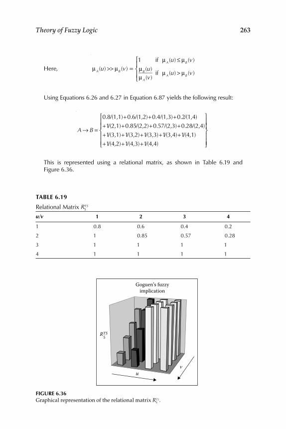
Theory of Fuzzy Logic 263

Here,

μA (u) >> μB (v) =1 if μA (u) ≤ μB (v)

μB (u)μA (v)

if μA (u) > μB (v)

⎧⎨⎪

⎩⎪

Using Equations 6.26 and 6.27 in Equation 6.87 yields the following result:

A → B =

0.8/(1,1)+0.6/(1,2)+0.4/(1,3)+0.2/(1,4)

+1/(2,1)+0.85/(2,2)+0.57/(2,3)+0.28/(2,4)

+1/(3,1)+1/(3,2)+1/(3,3)+1/(3,4)+1/(4,1)

+1/(4,2)+1/(4,3)+1/(4,4)

⎧

⎨⎪⎪

⎩⎪⎪

⎫

⎬⎪⎪

⎭⎪⎪

This is represented using a relational matrix, as shown in Table 6.19 and Figure 6.36.

Goguen’s fuzzyimplication

uv

RTS5

FIGURE 6.36Graphical representation of the relational matrix R

5TS.

TABLE 6.19

Relational Matrix R5TS

u/v 1 2 3 4

1 0.8 0.6 0.4 0.2

2 1 0.85 0.57 0.28

3 1 1 1 1

4 1 1 1 1

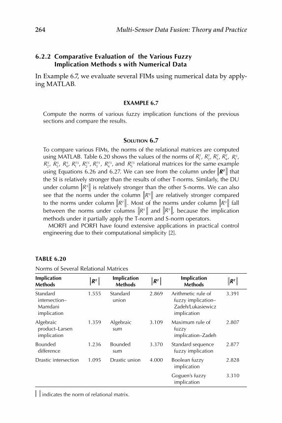
264 Multi-Sensor Data Fusion: Theory and Practice

6.2.2 Comparative Evaluation of the Various Fuzzy Implication Methods s with Numerical Data

In Example 6.7, we evaluate several FIMs using numerical data by apply-ing MATLAB.

EXAMPLE 6.7

Compute the norms of various fuzzy implication functions of the previous sections and compare the results.

SOLUTION 6.7To compare various FIMs, the norms of the relational matrices are computed using MATLAB. Table 6.20 shows the values of the norms of R1

T, R2T, R3

T, R4T, R1

S,R2

S, R3S, R4

S, R1TS, R2

TS, R3TS , R4

TS, and R5TS relational matrices for the same example

using Equations 6.26 and 6.27. We can see from the column under RT that the SI is relatively stronger than the results of other T-norms. Similarly, the DU under column RS is relatively stronger than the other S-norms. We can also see that the norms under the column RS are relatively stronger compared to the norms under column RT . Most of the norms under column RS fall between the norms under columns RT and RS , because the implication methods under it partially apply the T-norm and S-norm operators.

MORFI and PORFI have found extensive applications in practical control engineering due to their computational simplicity [2].

TABLE 6.20

Norms of Several Relational Matrices

Implication Methods

RT Implication Methods

RT Implication Methods

RT

Standard intersection–Mamdani implication

1.555 Standard union

2.869 Arithmetic rule of fuzzy implication–Zadeh/Lukasiewicz implication

3.391

Algebraic product–Larsen implication

1.359 Algebraic sum

3.109 Maximum rule of fuzzy implication–Zadeh

2.807

Bounded difference

1.236 Bounded sum

3.370 Standard sequence fuzzy implication

2.877

Drastic intersection 1.095 Drastic union 4.000 Boolean fuzzy implication

2.828

Goguen’s fuzzy implication

3.310

indicates the norm of relational matrix.

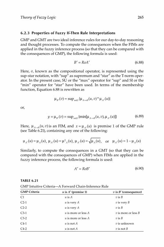
Theory of Fuzzy Logic 265

6.2.3 Properties of Fuzzy If-Then Rule Interpretations

GMP and GMT are two ideal inference rules for our day-to-day reasoning and thought processes. To compute the consequences when the FIMs are applied in the fuzzy inference process (so that they can be compared with the consequences of GMP), the following formula is used:

′B = Ro ′A (6.88)

Here, o, known as the compositional operator, is represented using the sup-star notation, with “sup” as supremum and “star” as the T-norm oper-ator. In the present case, SU or the “max” operator for “sup” and SI or the “min” operator for “star” have been used. In terms of the membership function, Equation 6.88 is rewritten as

μ ′B (v) = supu∈U {μA→B(u, v) * μ ′A (u)}

or,

y = μ ′B (v) = supu∈U {min[μA→B(u, v), μ ′A (u)]} (6.89)

Here, μA→B(u, v) is an FIM, and x = μ ′A (u) is premise 1 of the GMP rule

(see Table 6.21), containing any one of the following:

μ ′A (u) = μA (u), μ ′A (u) = μ2A (u), μ ′A (u) = μA (u), or μ ′A (u) = 1 − μA (u)

Similarly, to compute the consequences in a GMT (so that they can be compared with the consequences of GMP) when FIMs are applied in the fuzzy inference process, the following formula is used:

′A = Ro ′B (6.90)

TABLE 6.21

GMP Intuitive Criteria—A Forward Chain-Inference Rule

GMP Criteria u is A′ (premise 1) v is B′ (consequence)

C1 u is A v is B

C2-1 u is very A v is very B

C2-2 u is very A v is B

C3-1 u is more or less A v is more or less B

C3-2 u is more or less A v is B

C4-1 u is not A v is unknown

C4-2 u is not A v is not B

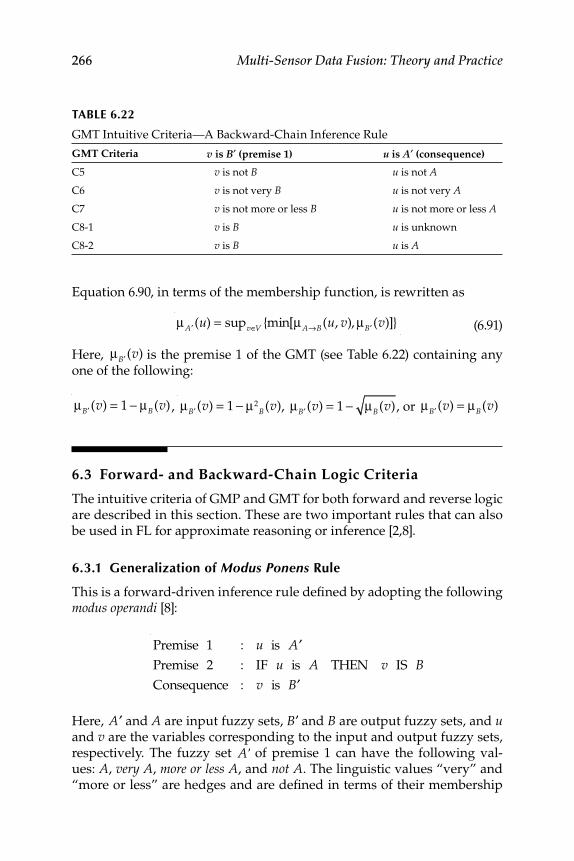
266 Multi-Sensor Data Fusion: Theory and Practice

Equation 6.90, in terms of the membership function, is rewritten as

μ ′A (u) = supv∈V {min[μA→B(u, v), μ ′B (v)]} (6.91)

Here, μ ′B (v) is the premise 1 of the GMT (see Table 6.22) containing any one of the following:

μ ′B (v) = 1 − μB(v), μ ′B (v) = 1 − μ2B(v),

μ ′B (v) = 1 − μB(v) , or μ ′B (v) = μB(v)

6.3 Forward- and Backward-Chain Logic Criteria

The intuitive criteria of GMP and GMT for both forward and reverse logic are described in this section. These are two important rules that can also be used in FL for approximate reasoning or inference [2,8].

6.3.1 Generalization of Modus Ponens Rule

This is a forward-driven inference rule defi ned by adopting the following modus operandi [8]:

Premise 1 : u is ′A

Premise 2 : IF u is A THEN v IS B

Consequence : v is ′B

Here, ′A and A are input fuzzy sets, ′B and B are output fuzzy sets, and u and v are the variables corresponding to the input and output fuzzy sets, respectively. The fuzzy set ′A of premise 1 can have the following val-ues: A, very A, more or less A, and not A. The linguistic values “very” and “more or less” are hedges and are defi ned in terms of their membership

TABLE 6.22

GMT Intuitive Criteria—A Backward-Chain Inference Rule

GMT Criteria v is B′ (premise 1) u is A′ (consequence)

C5 v is not B u is not A

C6 v is not very B u is not very A

C7 v is not more or less B u is not more or less A

C8-1 v is B u is unknown

C8-2 v is B u is A

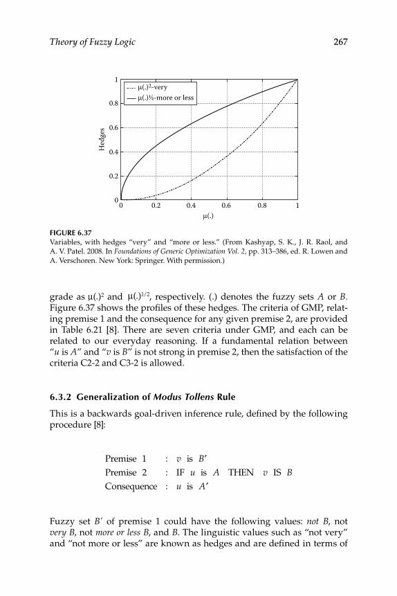
Theory of Fuzzy Logic 267

grade as μ(.)2 and μ(.)1/2, respectively. (.) denotes the fuzzy sets A or B. Figure 6.37 shows the profi les of these hedges. The criteria of GMP, relat-ing premise 1 and the consequence for any given premise 2, are provided in Table 6.21 [8]. There are seven criteria under GMP, and each can be related to our everyday reasoning. If a fundamental relation between “u is A” and “v is B” is not strong in premise 2, then the satisfaction of the criteria C2-2 and C3-2 is allowed.

6.3.2 Generalization of Modus Tollens Rule

This is a backwards goal-driven inference rule, defi ned by the following procedure [8]:

Premise 1 : v is ′B

Premise 2 : IF u is A THEN v IS B

Consequence : u is ′A

Fuzzy set B’ of premise 1 could have the following values: not B, not very B, not more or less B, and B. The linguistic values such as “not very” and “not more or less” are known as hedges and are defi ned in terms of

FIGURE 6.37Variables, with hedges “very” and “more or less.” (From Kashyap, S. K., J. R. Raol, and

A. V. Patel. 2008. In Foundations of Generic Optimization Vol. 2, pp. 313–386, ed. R. Lowen and

A. Verschoren. New York: Springer. With permission.)

1

0.8

0.6

0.4Hed

ges

0.2

0 0 0.2 0.4 0.6m(.)

0.8 1

m(.)½-more or lessm(.)2-very

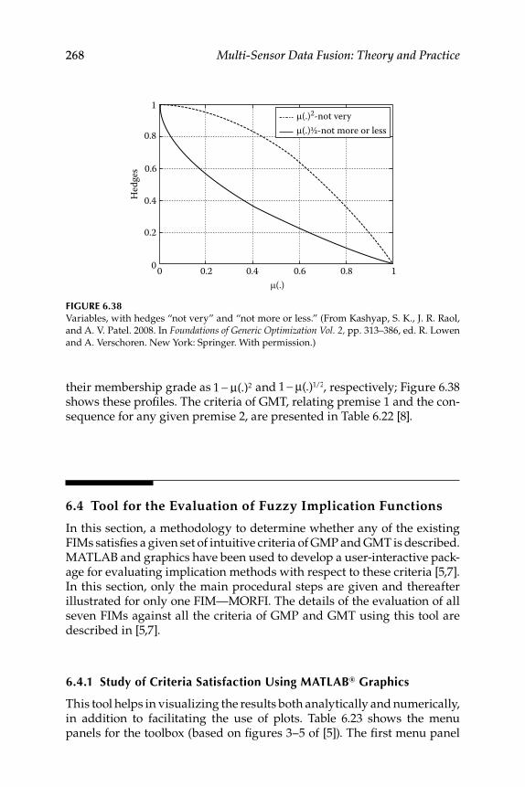
268 Multi-Sensor Data Fusion: Theory and Practice

their membership grade as 1 − μ(.)2 and 1 − μ(.)1/2, respectively; Figure 6.38 shows these profi les. The criteria of GMT, relating premise 1 and the con-sequence for any given premise 2, are presented in Table 6.22 [8].

6.4 Tool for the Evaluation of Fuzzy Implication Functions

In this section, a methodology to determine whether any of the existing FIMs satisfi es a given set of intuitive criteria of GMP and GMT is described. MATLAB and graphics have been used to develop a user-interactive pack-age for evaluating implication methods with respect to these criteria [5,7]. In this section, only the main procedural steps are given and thereafter illustrated for only one FIM—MORFI. The details of the evaluation of all seven FIMs against all the criteria of GMP and GMT using this tool are described in [5,7].

6.4.1 Study of Criteria Satisfaction Using MATLAB® Graphics

This tool helps in visualizing the results both analytically and numerically, in addition to facilitating the use of plots. Table 6.23 shows the menu panels for the toolbox (based on fi gures 3–5 of [5]). The fi rst menu panel

m(.)½-not more or lessm(.)2-not very

1

0.8

0.6

0.4Hed

ges

0.2

00 0.2 0.4 0.6m(.)

0.8 1

FIGURE 6.38Variables, with hedges “not very” and “not more or less.” (From Kashyap, S. K., J. R. Raol,

and A. V. Patel. 2008. In Foundations of Generic Optimization Vol. 2, pp. 313–386, ed. R. Lowen

and A. Verschoren. New York: Springer. With permission.)

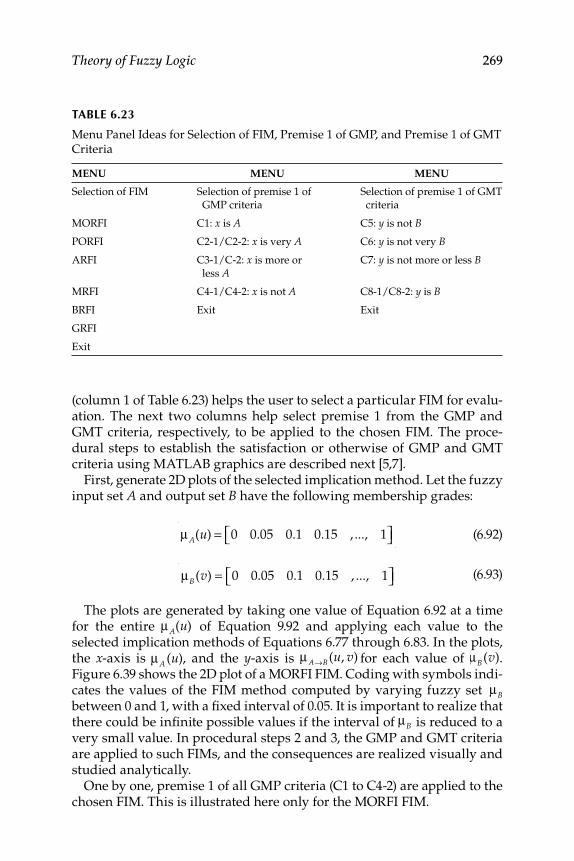
Theory of Fuzzy Logic 269

(column 1 of Table 6.23) helps the user to select a particular FIM for evalu-ation. The next two columns help select premise 1 from the GMP and GMT criteria, respectively, to be applied to the chosen FIM. The proce-dural steps to establish the satisfaction or otherwise of GMP and GMT criteria using MATLAB graphics are described next [5,7].

First, generate 2D plots of the selected implication method. Let the fuzzy input set A and output set B have the following membership grades:

μA(u) = 0 0.05 0.1 0.15 ,..., 1⎡⎣ ⎤⎦ (6.92)

μB(v) = 0 0.05 0.1 0.15 , ..., 1⎡⎣ ⎤⎦ (6.93)

The plots are generated by taking one value of Equation 6.92 at a time for the entire μA(u) of Equation 9.92 and applying each value to the selected implication methods of Equations 6.77 through 6.83. In the plots, the x-axis is μA (u), and the y-axis is μA→B(u, v) for each value of μB(v). Figure 6.39 shows the 2D plot of a MORFI FIM. Coding with symbols indi-cates the values of the FIM method computed by varying fuzzy set μB between 0 and 1, with a fi xed interval of 0.05. It is important to realize that there could be infi nite possible values if the interval of μB is reduced to a very small value. In procedural steps 2 and 3, the GMP and GMT criteria are applied to such FIMs, and the consequences are realized visually and studied analytically.

One by one, premise 1 of all GMP criteria (C1 to C4-2) are applied to the chosen FIM. This is illustrated here only for the MORFI FIM.

TABLE 6.23

Menu Panel Ideas for Selection of FIM, Premise 1 of GMP, and Premise 1 of GMT Criteria

MENU MENU MENU

Selection of FIM Selection of premise 1 of

GMP criteria

Selection of premise 1 of GMT

criteria

MORFI C1: x is A C5: y is not B

PORFI C2-1/C2-2: x is very A C6: y is not very B

ARFI C3-1/C-2: x is more or

less AC7: y is not more or less B

MRFI C4-1/C4-2: x is not A C8-1/C8-2: y is B

BRFI Exit Exit

GRFI

Exit

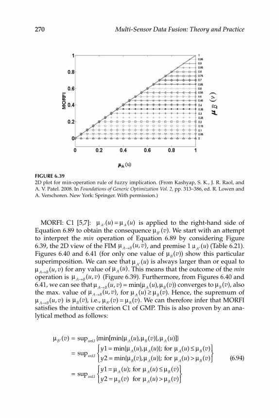
270 Multi-Sensor Data Fusion: Theory and Practice

MORFI: C1 [5,7]: μ ′A (u) = μA (u) is applied to the right-hand side of Equation 6.89 to obtain the consequence μ ′B (v). We start with an attempt to interpret the min operation of Equation 6.89 by considering Figure 6.39, the 2D view of the FIM μA→B(u, v), and premise 1 μ ′A (u) (Table 6.21). Figures 6.40 and 6.41 (for only one value of μB(v)) show this particular superimposition. We can see that μ ′A (u) is always larger than or equal to μA→B(u, v) for any value of μA (u). This means that the outcome of the min operation is μA→B(u, v) (Figure 6.39). Furthermore, from Figures 6.40 and 6.41, we can see that μA→B(u, v) = min(μA (u), μB(v)) converges to μB(v), also the max. value of μA→B(u, v), for μA (u) ≥ μB(v). Hence, the supremum of μA→B(u, v) is μB(v), i.e., μ ′B (v) = μB(v). We can therefore infer that MORFI satisfi es the intuitive criterion C1 of GMP. This is also proven by an ana-lytical method as follows:

μB ′ (v) = supu∈U {min[min{μA(u),μB(v)},μA (u)]}

= supu∈U

y1 = min{μA(u),μA(u)}; for μA(u) ≤ μB(v)

y2 = min{μB(v),μA(u)}; for μA(u) > μB(v)

⎧⎨⎩

⎫⎬⎭

= supu∈U

y1 = μA (u); for μA(u) ≤ μB(v)

y2 = μB(v) for μA(u) > μB(v)

⎧⎨⎩

⎫⎬⎭

(6.94)

FIGURE 6.392D plot for min-operation rule of fuzzy implication. (From Kashyap, S. K., J. R. Raol, and

A. V. Patel. 2008. In Foundations of Generic Optimization Vol. 2, pp. 313–386, ed. R. Lowen and

A. Verschoren. New York: Springer. With permission.)

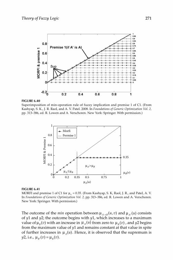
Theory of Fuzzy Logic 271

The outcome of the min operation between μA→B(u, v) and μ ′A (u) consists of y1 and y2; the outcome begins with y1, which increases to a maximum value of μB(v) with an increase in μA (u) from zero to μB(v) , and y2 begins from the maximum value of y1 and remains constant at that value in spite of further increases in μA(u) . Hence, it is observed that the supremum is y2, i.e., μ ′B (v) = μB(v).

FIGURE 6.41MORFI and premise 1 of C1 for μB = 0.35. (From Kashyap, S. K, Raol, J. R., and Patel, A. V.

In Foundations of Generic Optimization Vol. 2, pp. 313–386, ed. R. Lowen and A. Verschoren.

New York: Springer. With permission.)

MO

RFI &

Pre

mise

1

0.8

1

0.6

0.4

0.2

00 0.2 0.35 0.5 0.75 1

μA(u)

μB(v)

μA > μB

μA ≤ μB

0.35

MorfiPermise 1

FIGURE 6.40Superimposition of min-operation rule of fuzzy implication and premise 1 of C1. (From

Kashyap, S. K., J. R. Raol, and A. V. Patel. 2008. In Foundations of Generic Optimization Vol. 2, pp. 313–386, ed. R. Lowen and A. Verschoren. New York: Springer. With permission.)

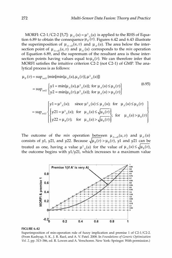
272 Multi-Sensor Data Fusion: Theory and Practice

MORFI: C2-1/C2-2 [5,7]: μ ′A (u) = μ2A (u) is applied to the RHS of Equa-

tion 6.89 to obtain the consequence μ ′B (v). Figures 6.42 and 6.43 illustrate the superimposition of μA→B(u, v) and μ ′A (u). The area below the inter-section point of μA→B(u, v) and

μ ′A (u) corresponds to the min operation of Equation 6.89, and the supremum of the resultant area is those inter-section points having values equal to μB(v). We can therefore infer that MORFI satisfi es the intuitive criterion C2-2 (not C2-1) of GMP. The ana-lytical process is as follows:

μB' (v) = supu∈U {min[min{μA (u),μB(v)},μ2A (u)]}

= supu∈U

y1 = min{μA (u),μ2A (u)}; for μA (u) ≤ μB(v)

y2 = min{μB(v),μ2A (u)}; for μA (u) > μB(v)

⎧⎨⎩

⎫⎬⎭

= supu∈U

y1 = μ2A (u); since μ2

A (u) ≤ μA (u); for μA (u) ≤ μB(v)

y21 = μ2A (u); for μA (u) ≤ μB(v)

y22 = μB(v); for μA (u) > μB(v)

⎧⎨⎪

⎩⎪

⎫⎬⎪

⎭⎪; for μA (u) > μB(v)

⎧

⎨⎪⎪

⎩⎪⎪

⎫

⎬⎪⎪

⎭⎪⎪

The outcome of the min operation between μA→B(u, v) and μ ′A (u)

consists of y1, y21, and y22. Because μB(v) > μB(v), y1 and y21 can be

treated as one, having a value μ2A (u) for the value of μA (u) ≤ μB(v),

the outcome begins with y1/y21, which increases to a maximum value

(6.95)

FIGURE 6.42Superimposition of min-operation rule of fuzzy implication and premise 1 of C2-1/C2-2.

(From Kashyap, S. K., J. R. Raol, and A. V. Patel. 2008. In Foundations of Generic Optimization Vol. 2, pp. 313–386, ed. R. Lowen and A. Verschoren. New York: Springer. With permission.)

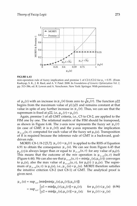
Theory of Fuzzy Logic 273

of μB(v) with an increase in μA (u) from zero to μB(v). The function y22 begins from the maximum value of y1/y21 and remains constant at that value in spite of any further increase in μA (u). Thus, we can see that the supremum is fi xed at y22, i.e., μ ′B (v) = μB(v).

Again, premise 1 of all GMT criteria, i.e., C5 to C8-2, are applied to the FIM one by one. The relational matrix of the FIM should be transposed, as shown in Figure 6.44. The x-axis now represents the fuzzy set μB(v) (in case of GMP, it is μA (u)) and the y-axis represents the implication μA→B(u, v) computed for each value of the fuzzy set μA(u). Transposition of R is required because the inference rule of GMT is a backward, goal-driven rule.

MORFI: C8-1/8-2 [5,7]: μ ′B (v) = μB(v) is applied to the RHS of Equation 6.91 to obtain the consequence μ ′A (u). We can see from Figure 6.45 that

μ ′B (v) is always larger than or equal to μA→B(u, v) for any value of μB(v).

This means that the outcome of the min operation is μA→B(u, v) itself (Figure 6.44). We can also see that μA→B(u, v) = min(μA (u), μB(v)) converges to μA(u), also the max value of μA→B(u, v), for μB(v) ≥ μA(u). The supre-mum of μA→B(u, v) is μA(u), i.e., μ ′A (u) = μA (u). MORFI therefore satisfi es the intuitive criterion C8-2 (not C8-1) of GMT. The analytical proof is given next.

μ ′A (u) = supv∈V {min[min(μA (u), μB(v)), μB(v)]}

= supv∈V

y1 = min[μB(v), μB(v)] = μB(v); for μB(v) ≤ μA (u)

y2 = min[μA (u), μB(v)] = μA (u); for μB(v) > μA (u)

⎧⎨⎩

(6.96)

FIGURE 6.43min-operation rule of fuzzy implication and premise 1 of C2-1/C2-2 for μB = 0.35 . (From

Kashyap, S. K., J. R. Raol, and A. V. Patel. 2008. In Foundations of Generic Optimization Vol. 2, pp. 313–386, ed. R. Lowen and A. Verschoren. New York: Springer. With permission.)

MO

RFI &

Pre

mise

1 0.8

1

0.6

0.4

0.2

00 0.25 0.4 0.59 0.75 1

μA(u)

μA ≤ √ μBμA > √ μB

μB(v)

0.35

MORFIPremise 1

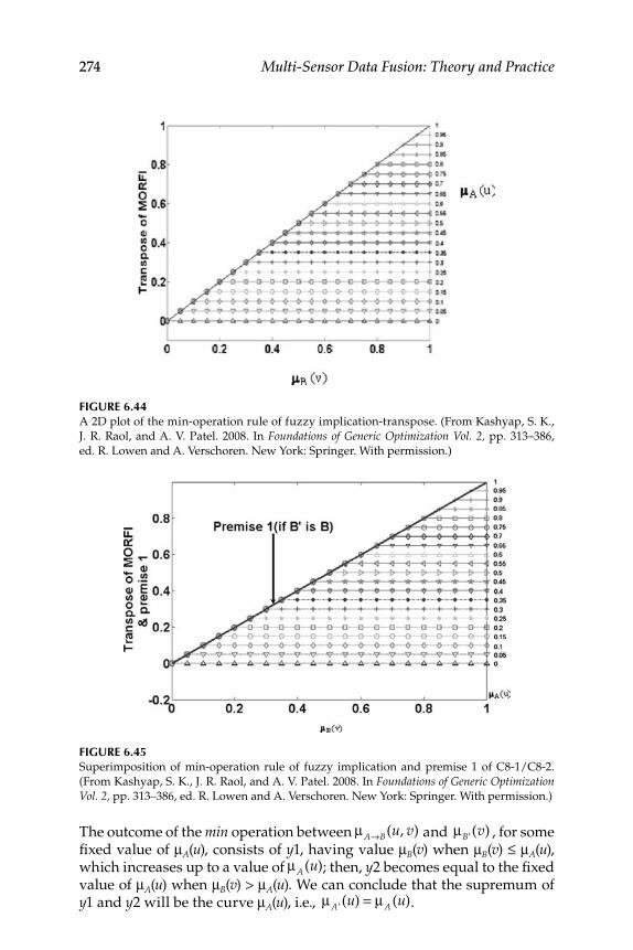
274 Multi-Sensor Data Fusion: Theory and Practice

The outcome of the min operation between μA→B(u, v) and μ ′B (v) , for some fi xed value of μA(u), consists of y1, having value μB(v) when μB(v) ≤ μA(u), which increases up to a value of μA (u); then, y2 becomes equal to the fi xed value of μA(u) when μB(v) > μA(u). We can conclude that the supremum of y1 and y2 will be the curve μA(u), i.e., μ ′A (u) = μA (u).

FIGURE 6.44A 2D plot of the min-operation rule of fuzzy implication-transpose. (From Kashyap, S. K.,

J. R. Raol, and A. V. Patel. 2008. In Foundations of Generic Optimization Vol. 2, pp. 313–386,

ed. R. Lowen and A. Verschoren. New York: Springer. With permission.)

FIGURE 6.45Superimposition of min-operation rule of fuzzy implication and premise 1 of C8-1/C8-2.

(From Kashyap, S. K., J. R. Raol, and A. V. Patel. 2008. In Foundations of Generic Optimization Vol. 2, pp. 313–386, ed. R. Lowen and A. Verschoren. New York: Springer. With permission.)

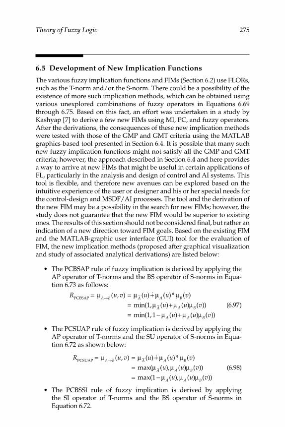
Theory of Fuzzy Logic 275

6.5 Development of New Implication Functions

The various fuzzy implication functions and FIMs (Section 6.2) use FLORs, such as the T-norm and/or the S-norm. There could be a possibility of the existence of more such implication methods, which can be obtained using various unexplored combinations of fuzzy operators in Equations 6.69 through 6.75. Based on this fact, an effort was undertaken in a study by Kashyap [7] to derive a few new FIMs using MI, PC, and fuzzy operators. After the derivations, the consequences of these new implication methods were tested with those of the GMP and GMT criteria using the MATLAB graphics-based tool presented in Section 6.4. It is possible that many such new fuzzy implication functions might not satisfy all the GMP and GMT criteria; however, the approach described in Section 6.4 and here provides a way to arrive at new FIMs that might be useful in certain applications of FL, particularly in the analysis and design of control and AI systems. This tool is fl exible, and therefore new avenues can be explored based on the intuitive experience of the user or designer and his or her special needs for the control-design and MSDF/AI processes. The tool and the derivation of the new FIM may be a possibility in the search for new FIMs; however, the study does not guarantee that the new FIM would be superior to existing ones. The results of this section should not be considered fi nal, but rather an indication of a new direction toward FIM goals. Based on the existing FIM and the MATLAB-graphic user interface (GUI) tool for the evaluation of FIM, the new implication methods (proposed after graphical visualization and study of associated analytical derivations) are listed below:

The PCBSAP• rule of fuzzy implication is derived by applying the AP operator of T-norms and the BS operator of S-norms in Equa-tion 6.73 as follows:

RPCBSAP

= μA→B(u, v) = μA (u) &+ μA (u) * μB(v)

= min(1,μA (u)+ μA (u)μB(v))

= min(1,1 − μA (u)+ μA (u)μB(v))

(6.97)

The PCSUAP rule of fuzzy implication is derived by applying the • AP operator of T-norms and the SU operator of S-norms in Equa-tion 6.72 as shown below:

RPCSUAP

= μA→B(u, v) = μA (u) &+ μA (u) * μB(v)

= max(μA (u),μA (u)μB(v))

= max(1 − μA (u),μA (u)μB(v))

(6.98)

The PCBSSI rule of fuzzy implication is derived by applying • the SI operator of T-norms and the BS operator of S-norms in Equation 6.72.

276 Multi-Sensor Data Fusion: Theory and Practice

RPCBSSI

= μA→B(u, v) = μA (u) &+ μA (u) * μB(v)

= μA (u) &+ min(μA (u),μB(v))

= min(1,1 − μA (u) + min(μA(u),μB(v)))

(6.99)

The PCBSBP rule of fuzzy implication is derived by applying the • BP operator of T-norms and the BS operator of S-norms in Equa-tion 6.72 as shown underneath:

RPCBSBP

= μA→B(u, v) = μA (u) &+ μA (u) * μB(v)

= min(1,μA (u) + max(0,μA (u) + μB(v) − 1))

= min(1,1 − μA

(u) + max(0,μA (u) + μB(v) − 1))

(6.100)

The PCSUBP rule of fuzzy implication is derived by applying the • BP operator of T-norms and the SU operator of S-norms in Equa-tion 6.72 as follows:

RPCSUBP

= μA→B(u, v) = μA (u) &+ μA (u) * μB(v)

= max(μA (u), max(0,μA

(u) + μB(v) − 1))

= max(1 − μA (u), max(0,μA (u) + μB(v) − 1))

(6.101)

The PCASBP rule of fuzzy implication is derived by applying the • BP operator of T-norms and the AS operator of S-norms in Equa-tion 6.72 to yield the following:

RPCASBP

= μA→B(u, v) = μA (u) &+ μA (u) * μB(v)

= 1 − μA (u) + max(0,μA (u) + μB(v) − 1)

− (1 − μA (u))max(0,μA (u) + μB(v) − 1)

(6.102)

The PCASAP rule of fuzzy implication is derived by applying the • AP operator of T-norms and the AS operator of S-norms in Equa-tion 6.72 as represented below:

RPCASAP

= μA→B(u, v) = μA (u) &+ μA (u) * μB(v)

= 1 − μA (u) + μA (u)μB(v) − (1 − μA (u))μA (u)μB(v)

= 1 − μA (u) + μA (u)μB(v) − μA (u)μB(v) + μ2A (u)μB(v)

= 1 − μA (u)(1 − μA (u)μB(v))

(6.103)

Theory of Fuzzy Logic 277

The PCASSI rule of fuzzy implication is derived by applying • the SI operator of T-norms and the AS operator of S-norms in Equation 6.72.

RPCASAP

μA→B(u, v) = μA (u) &+ μA (u) * μB(v)

= 1 − μA (u) + min(μA (u),μB(v))

= 1 − μA (u) + min(μA (u),μB(v))

− (1 − μA (u))min(μA (u), μ(v))

= 1 − μA (u) + min(μA (u),μB(v))

− min( μA (u),μB(v)) + μA (u)min(μA (u), μB(v))

= 1 − μA (u)(1 − min(μA (u),μB(v)))

(6.104)

The MIAS rule of fuzzy implication is derived by applying the AS • operator of S-norms in Equation 6.71 as depicted below:

RMIAS

= μA→B(u, v) = μA (u) &+ μB(v)

= 1 − μA (u) + μB(v) − (1 − μA (u))μB(v)

= 1 − μA (u) + μB(v) − μB(v) + μA (u)μB(v)

= 1 − μA (u)(1 − μB(v))

(6.105)

The procedural steps used to generate the 2D plots of new implication methods are the same as those discussed in Section 6.4. Some modifi ca-tion is carried out in the existing MATLAB graphics tool by adding new cases to existing cases and writing the mathematical equations pertain-ing to any of the new implication methods, to derive these implication methods and conduct their “satisfaction” studies by checking against the intuitive criteria of the GMP and GMT rules. At this point, it is important to mention that the various implication methods discussed in Section 6.4 and this section might not be applicable to all types of applications, and it is up to any domain expert to select an appropriate method suitable for a particular application. The user can cut down the effort level by fi rst considering those implication methods that satisfy the maximum number of intuitive criteria of GMP and GMT. For the purpose of illustration, only one new FIM (from the list above) is considered, and the discussion is cen-tered on the criteria that are satisfi ed by the selected FIM; all new FIMs do not satisfy all the criteria, and the discussions related to this aspect are not repeated in the present book. The complete details can be found in works by Kashyap [7]. The purpose here is to illustrate how a new FIM can be evolved and evaluated using the same MATLAB GUI tool, as explained in

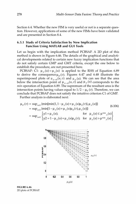
278 Multi-Sensor Data Fusion: Theory and Practice

Section 6.4. Whether the new FIM is very useful or not is a separate ques-tion. However, applications of some of the new FIMs have been validated and are presented in Section 8.4.

6.5.1 Study of Criteria Satisfaction by New Implication Function Using MATLAB and GUI Tools

Let us begin with the implication method PCBSAP. A 2D plot of this method is shown in Figure 6.46. The details of the graphical and analyti-cal developments related to certain new fuzzy implication functions that do not satisfy certain GMP and GMT criteria, except the one below to establish the procedure, are not presented here.

PCBSAP: C1: μ ′A (u) = μA (u) is applied to the RHS of Equation 6.89 to derive the consequence μ ′B (v). Figures 6.47 and 6.48 illustrate the superimposed plots of μA→B(u, v) and μ ′A (u). We can see that the area below the intersection point of μA→B(u, v) and μ ′A (u) corresponds to the min operation of Equation 6.89. The supremum of the resultant area is the intersection points having values equal to 1/2 − μB (v). Therefore, we can conclude that PCBSAP does not satisfy the intuitive criterion C1 of GMP.

Further analysis is elaborated next:

μ ′B (v) = supu∈U {min[min{1,1 − μA (u) + μA (u)μB(v)},μA (u)]}

= supu∈U {min[1 − μA (u) + μA (u)μB(v),μA (u)]}

= supu∈U

y1 = μA (u); for μA (u) ≤ μminA (u)

y2 = 1 − μA (u) + μA (u)μB(v); for μA (u) > μminA (u)

⎧⎨⎩

⎫⎬⎭

(6.106)

FIGURE 6.46 2D plots of PCBSAP.

)v(B

)(uA

0.2

μ

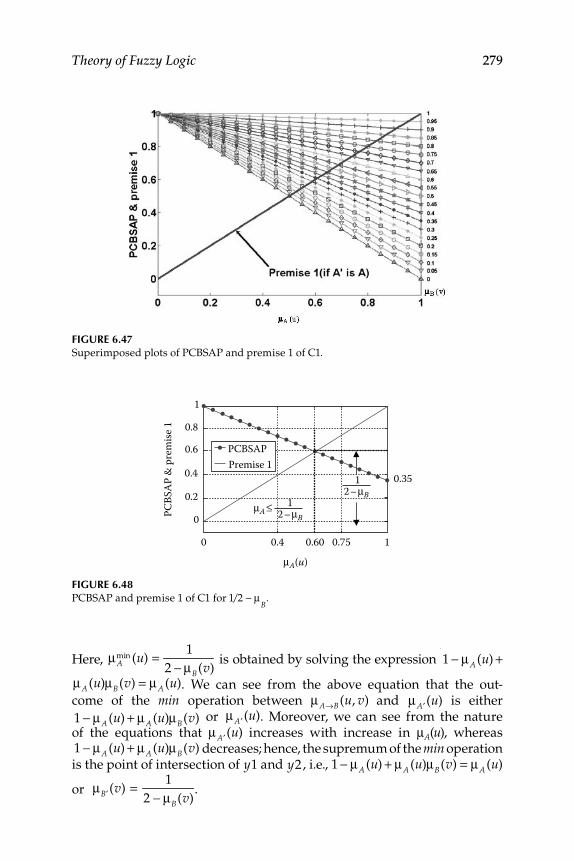
Theory of Fuzzy Logic 279

Here, μAmin (u) = 1

2 − μB(v) is obtained by solving the expression

1 − μA (u) +

μA (u)μB(v) = μA (u). We can see from the above equation that the out-come of the min operation between μA→B(u, v) and μ ′A (u) is either

1 − μA (u) + μA (u)μB(v) or μ ′A (u). Moreover, we can see from the nature of the equations that μ ′A (u) increases with increase in μA(u), whereas

1 − μA (u) + μA (u)μB(v) decreases; hence, the supremum of the min operation is the point of intersection of y1 and y2, i.e., 1 − μA (u) + μA (u)μB(v) = μA (u)

or μ ′B (v) = 1

2 − μB(v).

FIGURE 6.47 Superimposed plots of PCBSAP and premise 1 of C1.

FIGURE 6.48PCBSAP and premise 1 of C1 for 1/2 − μ

B.

2–μB1

2–μB1

PCBS

AP

& p

rem

ise 1 0.8

1

0.6

0.4

0.2

0

0 0.4 0.60 0.75 1

μA(u)

μA ≤

0.35

PCBSAPPremise 1

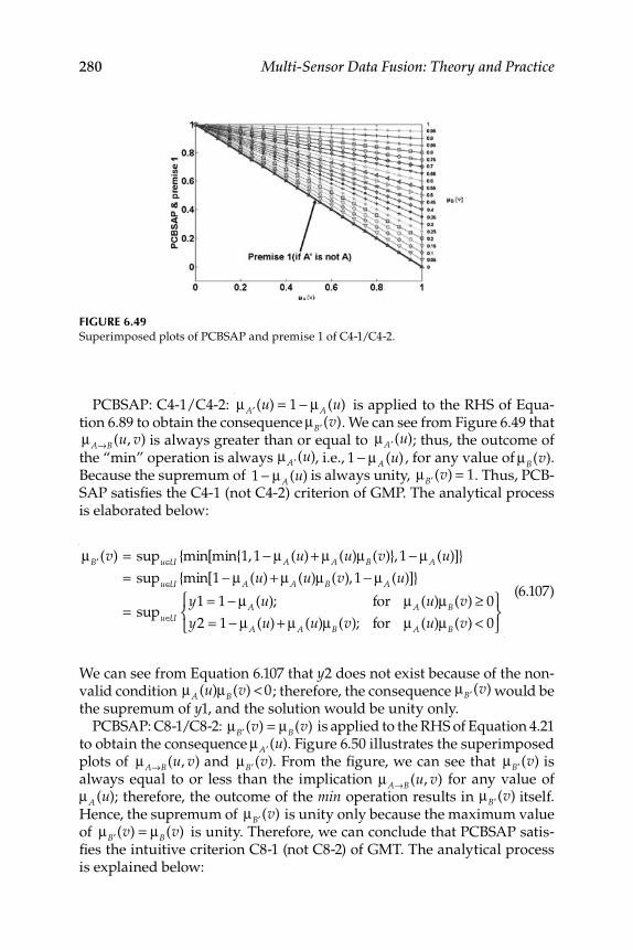
280 Multi-Sensor Data Fusion: Theory and Practice

PCBSAP: C4-1/C4-2: μ ′A (u) = 1 − μA (u) is applied to the RHS of Equa-tion 6.89 to obtain the consequence μ ′B (v). We can see from Figure 6.49 that μA→B(u, v) is always greater than or equal to μ ′A (u); thus, the outcome of the “min” operation is always μ ′A (u), i.e., 1 − μA (u) , for any value of μB(v). Because the supremum of 1 − μA (u) is always unity, μ ′B (v) = 1. Thus, PCB-SAP satisfi es the C4-1 (not C4-2) criterion of GMP. The analytical process is elaborated below:

μ ′B (v) = supu∈U {min[min{1,1 − μA (u) + μA (u)μB(v)},1 − μA (u)]}

= supu∈U {min[1 − μA (u) + μA (u)μB(v),1 − μA (u)]}

= supu∈U

y1 = 1 − μA (u); for μA (u)μB(v) ≥ 0

y2 = 1 − μA (u) + μA (u)μB(v); for μA (u)μB(v) < 0

⎧⎨⎩

⎫⎬⎭

(6.107)

We can see from Equation 6.107 that y2 does not exist because of the non-valid condition μA (u)μB(v) < 0; therefore, the consequence μ ′B (v) would be the supremum of y1, and the solution would be unity only.

PCBSAP: C8-1/C8-2: μ ′B (v) = μB(v) is applied to the RHS of Equation 4.21 to obtain the consequence μ ′A (u). Figure 6.50 illustrates the superimposed plots of μA→B(u, v) and μ ′B (v). From the fi gure, we can see that μ ′B (v) is always equal to or less than the implication μA→B(u, v) for any value of μA (u); therefore, the outcome of the min operation results in μ ′B (v) itself. Hence, the supremum of μ ′B (v) is unity only because the maximum value of μ ′B (v) = μB(v) is unity. Therefore, we can conclude that PCBSAP satis-fi es the intuitive criterion C8-1 (not C8-2) of GMT. The analytical process is explained below:

FIGURE 6.49 Superimposed plots of PCBSAP and premise 1 of C4-1/C4-2.

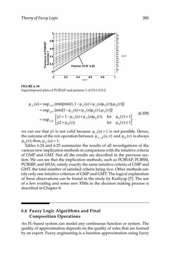
Theory of Fuzzy Logic 281

μ ′A (u) = supv∈V {min[min(1,1 − μA (u) + μA (u)μB(v)),μB(v)]}

= supv∈V {min[1 − μA (u) + μA (u)μB(v),μB(v)]}

= supv∈V

y1 = 1 − μA (u) + μA (u)μB(v); for μB(v) > 1

y2 = μB(v); for μB(v) ≤ 1

⎧⎨⎩

⎫⎬⎭

(6.108)

we can see that y1 is not valid because μA (u) > 1 is not possible. Hence, the outcome of the min operation between μA→B(u, v) and μ ′B (v) is always μB(v); thus, μ ′A (u) = 1.

Tables 6.24 and 6.25 summarize the results of all investigations of the various new implication methods in comparison with the intuitive criteria of GMP and GMT. Not all the results are described in the previous sec-tion. We can see that the implication methods, such as PCBSAP, PCBSSI, PCBSBP, and MIAS, satisfy exactly the same intuitive criteria of GMP and GMT, the total number of satisfi ed criteria being two. Other methods sat-isfy only one intuitive criterion of GMP and GMT. The logical explanation of these observations can be found in the study by Kashyap [7]. The use of a few existing and some new FIMs in the decision making process is described in Chapter 8.

6.6 Fuzzy Logic Algorithms and Final

Composition Operations

An FL-based system can model any continuous function or system. The quality of approximation depends on the quality of rules that are formed by an expert. Fuzzy engineering is a function approximation using fuzzy

FIGURE 6.50Superimposed plots of PCBSAP and premise 1 of C8-1/C8-2.

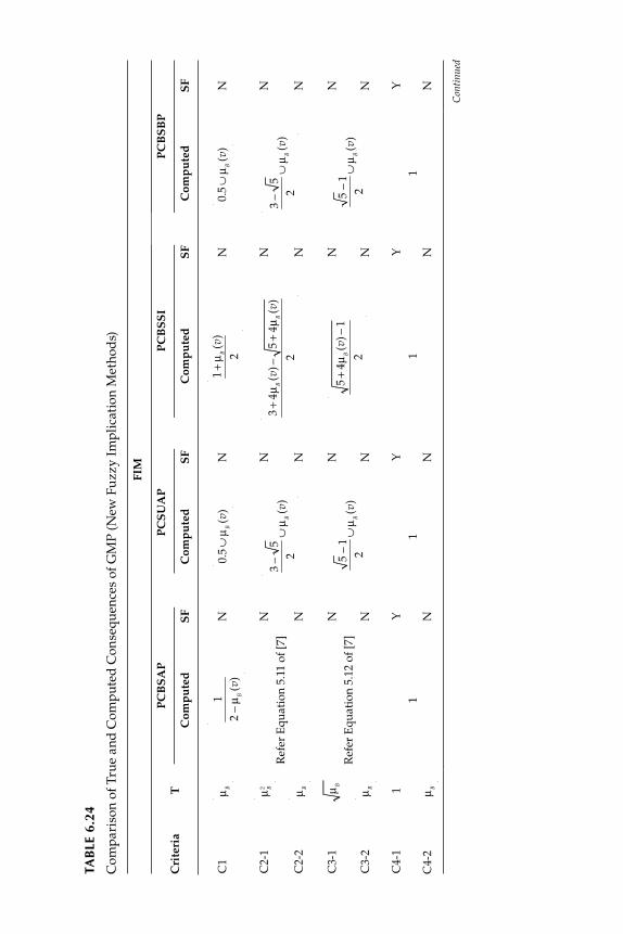
Con

tinu

ed

TAB

LE 6

.24

Co

mp

ari

son

of

Tru

e a

nd

Co

mp

ute

d C

on

seq

uen

ces

of

GM

P (

New

Fu

zz

y I

mp

lica

tio

n M

eth

od

s)

FIM

Cri

teri

aT

PC

BS

AP

PC

SU

AP

PC

BS

SI

PC

BS

BP

Co

mp

ute

dS

FC

om

pu

ted

SF

Co

mp

ute

dS

FC

om

pu

ted

SF

C1

μ B

1

2−

μ B(v

)N

0.5

∪μ B

(v)

N

1+

μ B(v

)

2N

0.5

∪μ B

(v)

N

C2-1

μ B2

Ref

er E

qu

ati

on

5.1

1 o

f [7

]

N

3−

5

2∪

μ B(v

)

N

3+

4μ B

(v)−

5+

4μ B

(v)

2

N

3−

5

2∪

μ B(v

)

N

C2-2

μ BN

NN

N

C3-1

μ B

Ref

er E

qu

ati

on

5.1

2 o

f [7

]

N5

−1

2∪

μ B(v

)

N

5+

4μ B

(v)−

1

2

N5

−1

2∪

μ B(v

)

N

C3-2

μ BN

NN

N

C4-1

1

1

Y

1

Y

1

Y

1

Y

C4-2

μ BN

NN

N

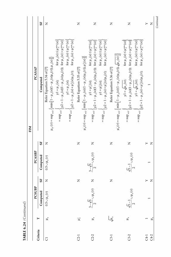
TAB

LE 6

.24

(Con

tinue

d)

FIM

Cri

teri

aT

PC

SU

BP

PC

AS

BP

PC

AS

AP

Co

mp

ute

dS

FC

om

pu

ted

SF

Co

mp

ute

dS

F

C1

μ B 0

.5∪

μ B(v

)N

0.5

∪μ B

(v)

NR

efer

Eq

uati

on

5.3

4 o

f [7

]

μ B′(

v)=

sup

u∈U

min

1−

μA(u

)(1

−μ

A(u

)μB(v

)),μ

A(u

)⎡ ⎣

⎤ ⎦{

}=

sup

u∈U

y1=

μA

(u);

for

μA(u

)≤

μAm

in(u

)

y2=

1−

μA(u

)(1

−μ

A(u

)μB(v

));

for

μA(u

)>

μAm

in(u

)

⎧ ⎨ ⎩

⎫ ⎬ ⎭

=su

pu∈

U

y1=

μA(u

);fo

r μ

A(u

)≤

μAm

in(u

)

y2=

1−

μA(u

)+

μA2(u

)μB(v

);fo

r μ

A(u

)>

μAm

in(u

)

⎧ ⎨ ⎩

⎫ ⎬ ⎭

N

C2-1

μ B2

3−

5

2∪

μ B(v

)

N

3−

5

2∪

μ B(v

)

NR

efer

Eq

uati

on

5.3

5 o

f [7

]N

C2-2

μ BN

N

μ B′(v

)=

sup

u∈U

min

1−

μA(u

)(1

−μ

A(u

)μB(v

)),μ

A2(u

)⎡ ⎣

⎤ ⎦{

}=

sup

u∈U

y1=

μA2

(u);

for

μA(u

)≤

μAm

in(u

)

y2=

1−

μA(u

)(1

−μ

A(u

)μB(v

));

for

μA(u

)>

μAm

in(u

)

⎧ ⎨ ⎩

⎫ ⎬ ⎭

=su

pu∈

U

y1=

μA2(u

);fo

r μ

A(u

)≤

μAm

in(u

)

y2=

1−

μA(u

)+

μA2(u

)μB(v

);fo

r μ

A(u

)>

μAm

in(u

)

⎧ ⎨ ⎩

⎫ ⎬ ⎭

N

C3-1

μ B

5−

1

2∪

μ B(v

)

N

5−

1

2∪

μ B(v

)

NR

efer

Eq

uati

on

5.3

6 o

f [7

]N

C3-2

μ BN

μ B′(v

)=

sup

u∈U

min

1−

μA(u

)(1

−μ

A(u

)μB(v

)),

μA

(u)

⎡ ⎣⎤ ⎦

{}

=su

pu∈

U

y1=

μA

(u);

for

μA(u

)≤

μAm

in(u

)

y2=

1−

μA(u

)(1

−μ

A(u

)μB(v

));

for

μA(u

)>

μAm

in(u

)

⎧ ⎨⎪ ⎩⎪

⎫ ⎬⎪ ⎭⎪

=su

pu∈

U

y1=

μA(u

);fo

r μ

A(u

)≤

μAm

in(u

)

y2=

1−

μA(u

)+

μA2(u

)μB(v

);fo

r μ

A(u

)>

μAm

in(u

)

⎧ ⎨⎪ ⎩⎪

⎫ ⎬⎪ ⎭⎪

N

C4-1

11

Y1

Y1

Y

C4-2

μ BN

NN

Con

tinu

ed

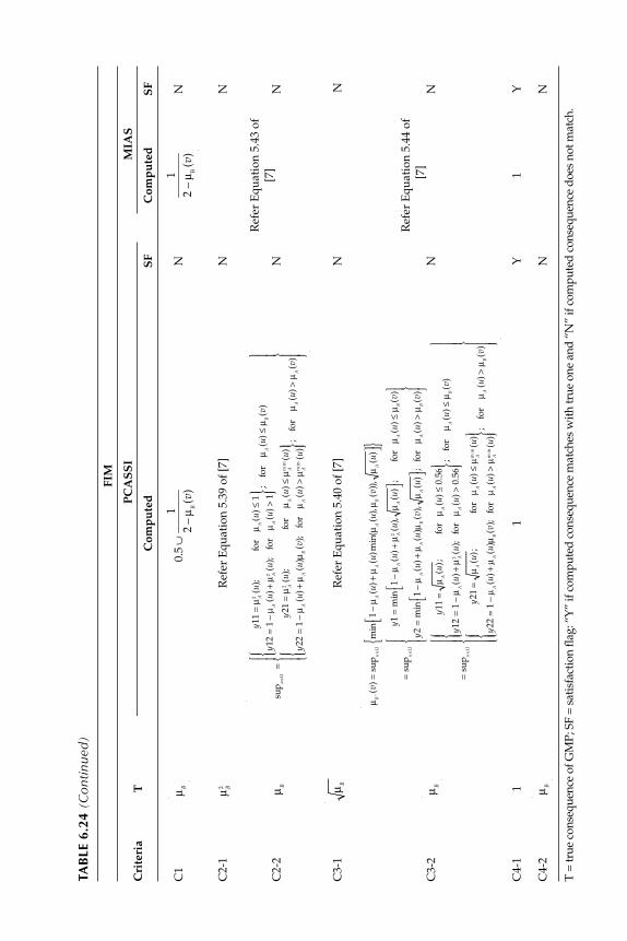
TAB

LE 6

.24

(Con

tinue

d)

FIM

Cri

teri

aT

PC

AS

SI

MIA

S

Co

mp

ute

dS

FC

om

pu

ted

SF

C1

μ B0.5

∪1

2−

μ B(v

)N

1

2−

μ B(v

)N

C2-1

μ B2R

efer

Eq

uati

on

5.3

9 o

f [7

]N

Ref

er E

qu

ati

on

5.4

3 o

f

[7]

N

C2-2

μ B

sup

u∈U

=

y11

=μ

A2(u

);fo

rμ

A(u

)≤

1

y12

=1

−μ

A(u

)+

μA2

(u);

for

μA(u

)>

1

⎧ ⎨⎪ ⎩⎪

⎫ ⎬⎪ ⎭⎪;

for

μA(u

)≤

μ B(v

)

y21

=μ A2

(u);

for

μA(u

)≤

μAm

in(u

)

y22

=1

−μ

A(u

)+

μA

(u)μ

B(v

);fo

rμ

A(u

)>

μAm

in(u

)

⎧ ⎨⎪ ⎩⎪

⎫ ⎬⎪ ⎭⎪;

for

μA(u

)>

μA(v

)

⎧ ⎨⎪ ⎪ ⎩⎪ ⎪

⎫ ⎬⎪ ⎪ ⎭⎪ ⎪

NN

C3-1

μ BR

efer

Eq

uati

on

5.4

0 o

f [7

]N

Ref

er E

qu

ati

on

5.4

4 o

f

[7]

N

C3-2

μ B

μ B′(

v)=

sup

u∈U

min

1−

μA(u

)+

μA(u

)min

(μA(u

),μ B

(v))

,μ

A(u

)⎡ ⎣

⎤ ⎦{

}=

sup

u∈U

y1=

min

1−

μA(u

)+

μA2(u

),μ

A(u

)⎡ ⎣

⎤ ⎦;fo

rμ

A(u

)≤

μ B(v

)

y2=

min

1−

μA(u

)+

μA(u

)μB(v

),μ

A(u

)⎡ ⎣

⎤ ⎦;fo

rμ

A(u

)>

μ B(v

)

⎧ ⎨⎪ ⎩⎪

⎫ ⎬⎪ ⎭⎪

=su

pu

∈U

y11

=μ

A(u

);fo

rμ

A(u

)≤

0.5

6

y12

=1

−μ

A(u

)+

μA2(u

);fo

rμ

A(u

)>

0.5

6

⎧ ⎨⎪ ⎩⎪

⎫ ⎬⎪ ⎭⎪;

for

μA(u

)≤

μ B(v

)

y21

=μ A

(u);

for

μA(u

)≤

μAm

in(u

)

y22

=1

−μ

A(u

)+

μA(u

)μB(v

);fo

rμ

A(u

)>

μAm

in(u

)

⎧ ⎨⎪ ⎩⎪

⎫ ⎬⎪ ⎭⎪;

for

μA

(u)

>μ B

(v)

⎧ ⎨⎪ ⎪ ⎪ ⎩⎪ ⎪ ⎪

⎫ ⎬⎪ ⎪ ⎪ ⎭⎪ ⎪ ⎪

NN

C4-1

11

Y1

Y

C4-2

μ BN

N

T =

tru

e co

nse

qu

ence

of

GM

P; S

F =

sat

isfa

ctio

n fl

ag

: “Y

” if

co

mp

ute

d c

on

seq

uen

ce m

atch

es w

ith

tru

e o

ne

and

“N

” if

co

mp

ute

d c

on

seq

uen

ce d

oes

no

t m

atch

.

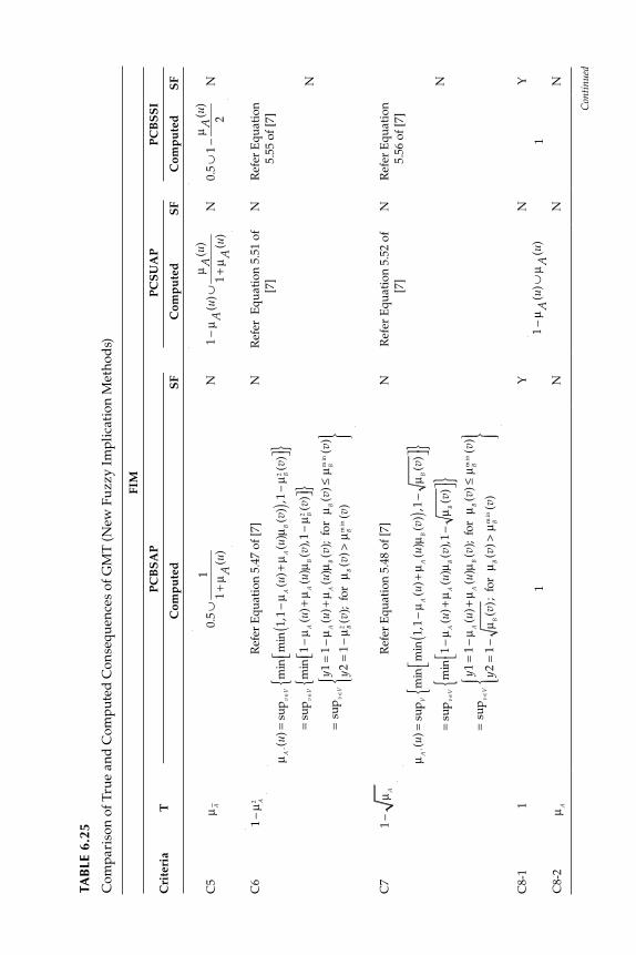
TAB

LE 6

.25

Co

mp

ari

son

of

Tru

e a

nd

Co

mp

ute

d C

on

seq

uen

ces

of

GM

T (

New

Fu

zz

y I

mp

lica

tio

n M

eth

od

s)

FIM

Cri

teri

aT

PC

BS

AP

PC

SU

AP

PC

BS

SI

Co

mp

ute

dS

FC

om

pu

ted

SF

Co

mp

ute

dS

F

C5

μA

0.5

∪1

1+

μA

(u)

N

1−

μA

(u)∪

μA

(u)

1+

μA

(u)

N 0

.5∪

1−

μA

(u)

2N

C6

1−

μA2

Ref

er E

qu

ati

on

5.4

7 o

f [7

]

μA

′(u)

=su

pv

∈V

min

min

1,1

−μ

A(u

)+μ

A(u

)μB(v

)(

),1−

μ B2(v

)⎡ ⎣

⎤ ⎦{

}=

sup

v∈

Vm

in1

−μ

A(u

)+μ

A(u

)μB(v

),1

−μ B2

(v)

⎡ ⎣⎤ ⎦

{}

=su

pv

∈V

y1=

1−

μA

(u)+

μA

(u)μ

B(v

);fo

rμ B

(v)

≤μ Bm

in(v

)

y2=

1−

μ B2(v

);fo

rμ B

(v)

>μ Bm

in(v

)

⎧ ⎨⎪ ⎩⎪

⎫ ⎬⎪ ⎭⎪

NR

efer

E

qu

ati

on

5.5

1 o

f

[7]

NR

efer

Eq

uati

on

5.5

5 o

f [7

]

N

C7

1−

μA

Ref

er E

qu

ati

on

5.4

8 o

f [7

]

μA

′(u)

=su

pV

min

min

1,1

−μ

A(u

)+μ

A(u

)μB(v

)(

),1−

μ B(v

)⎡ ⎣

⎤ ⎦{

}=

sup

v∈

Vm

in1

−μ

A(u

)+μ

A(u

)μB(v

),1

−μ B

(v)

⎡ ⎣⎤ ⎦

{}

=su

pv

∈V

y1=

1−

μA

(u)+

μA

(u)μ

B(v

);fo

rμ B

(v)

≤μ Bm

in(v

)

y2=

1−

μ B(v

);fo

rμ B

(v)

>μ Bm

in(v

)

⎧ ⎨⎪ ⎩⎪

⎫ ⎬⎪ ⎭⎪

NR

efer

Eq

uati

on

5.5

2 o

f

[7]

NR

efer

Eq

uati

on

5.5

6 o

f [7

]

N

C8-1

1

1

Y

1−

μA

(u)∪

μA

(u)

N

1

Y

C8-2

μA

NN

N

Con

tinu

ed

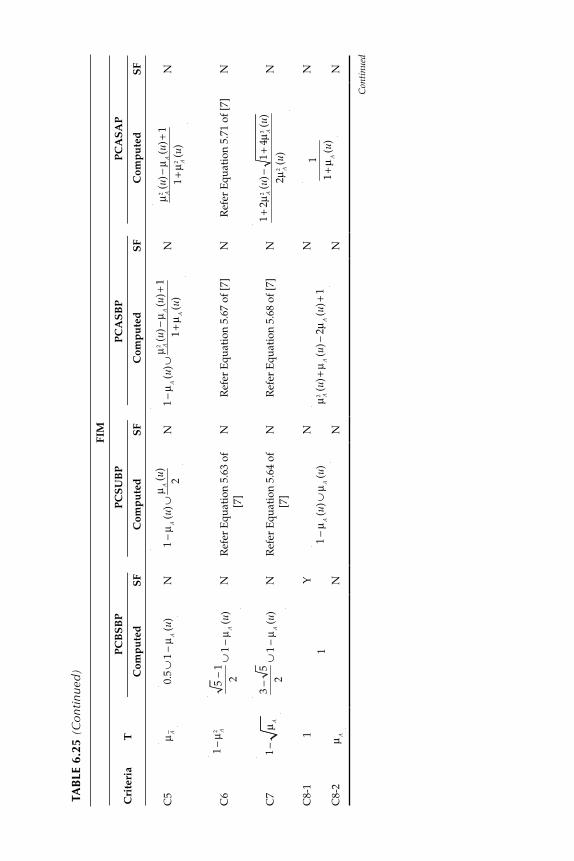
TAB

LE 6

.25

(Con

tinue

d)

FIM

Cri

teri

aT

PC

BS

BP

PC

SU

BP

PC

AS

BP

PC

AS

AP

Co

mp

ute

dS

FC

om

pu

ted

SF

Co

mp

ute

dS

FC

om

pu

ted

SF

C5

μA

0.5

∪1

−μ

A(u

)N

1−

μA

(u)∪

μA

(u)

2N

1−

μA

(u)∪

μA2

(u)−

μA

(u)+

1

1+

μA

(u)

N

μA2

(u)−

μA

(u)+

1

1+

μ A2(u

)N

C6

1−

μA2

5−

1

2∪

1−

μA

(u)

NR

efer

Eq

uati

on

5.6

3 o

f

[7]

NR

efer

Eq

uati

on

5.6

7 o

f [7

]N

Ref

er E

qu

ati

on

5.7

1 o

f [7

]N

C7

1−

μA

3−

5

2∪

1−

μA

(u)

NR

efer

Eq

uati

on

5.6

4 o

f

[7]

NR

efer

Eq

uati

on

5.6

8 o

f [7

]N

1+

2μ

A2(u

)−1

+4μ

A3(u

)

2μ

A2(u

)N

C8-1

1

1

Y

1−

μA

(u)∪

μA

(u)

N

μA2

(u)+

μA

(u)−

2μ

A(u

)+1

N

1

1+

μA

(u)

N

C8-2

μA

NN

NN

Con

tinu

ed

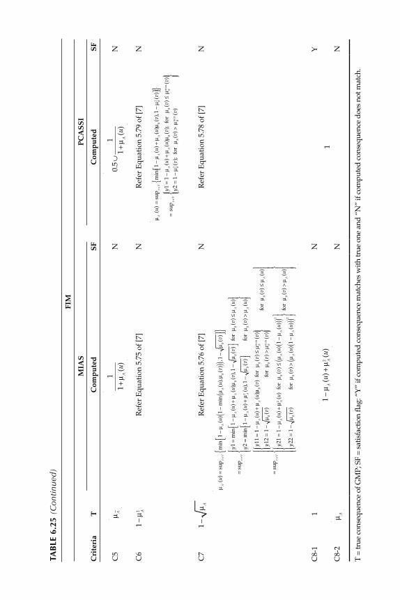
TAB

LE 6

.25

(Con

tinue

d)

FIM

T

MIA

SP

CA

SS

I

Cri

teri

aC

om

pu

ted

SF

Co

mp

ute

dS

F

C5

μA

1

1+

μA

(u)

N

0.5

∪1

1+

μA

(u)

N

C6

1−

μA2

Ref

er E

qu

ati

on

5.7

5 o

f [7

]N

Ref

er E

qu

ati

on

5.7

9 o

f [7

]

μA

′(u)

=su

pv

∈V

min

1−

μA

(u)

+μ

A(u

)μB(v

),1

−μ B2

(v)

⎡ ⎣⎤ ⎦

{}

=su

pv

∈V

y1=

1−

μA

(u)

+μ

A(u

)μB(v

);fo

rμ B

(v)

≤μ Bm

in(v

)

y2=

1−

μ B2(v

);fo

rμ B

(v)

>μ Bm

in(v

)

⎧ ⎨⎪ ⎩⎪

⎫ ⎬⎪ ⎭⎪

N

C7

1−

μA

Ref

er E

qu

ati

on

5.7

6 o

f [7

]

μA

′(u)

=su

pv

∈V

min

1−

μA

(u)

1−

min

μA

(u),

μ B(v

)(

)(

),1−

μ B(v

)⎡ ⎣

⎤ ⎦{

}=

sup

v∈

V

y1=

min

1−

μA

(u)

+μ

A(u

)μB(v

),1

−μ B

(v)

⎡ ⎣⎤ ⎦

for

μ B(v

)≤

μA

(u)

y2=

min

1−

μA

(u)

+μ

A2(u

),1

−μ B

(v)

⎡ ⎣⎤ ⎦

for

μ B(v

)>

μA

(u)

⎧ ⎨⎪ ⎩⎪

⎫ ⎬⎪ ⎭⎪

=su

pv

∈V

y11

=1

−μ

A(u

)+

μA

(u)μ

B(v

)fo

rμ B

(v)

≤μ Bm

in(v

)

y12

=1

−μ B

(v)

for

μ B(v

)>

μ Bmin

(v)

⎧ ⎨⎪ ⎩⎪

⎫ ⎬⎪ ⎭⎪fo

rμ B

(v)

≤μ

A(u

)

y21

=1

−μ

A(u

)+

μA2

(u)

for

μ B(v

)≤

μA

(u)

1−

μA

(u)

()

()2

y22

=1

−μ B

(v)

for

μ B(v

)>

μA

(u)

1−

μA

(u)

()

()2

⎧ ⎨⎪ ⎩⎪

⎫ ⎬⎪ ⎭⎪fo

rμ B

(v)

>μ

A(u

)

⎧ ⎨⎪ ⎪ ⎪ ⎩⎪ ⎪ ⎪

⎫ ⎬⎪ ⎪ ⎪ ⎭⎪ ⎪ ⎪

NR

efer

Eq

uati

on

5.7

8 o

f [7

]N

C8-1

1

1−

μA

(u)

+μ

A2(u

)

N

1

Y

C8-2

μA

NN

T =

tru

e co

nse

qu

ence

of

GM

P; S

F =

sat

isfa

ctio

n fl

ag

: “Y

” if

co

mp

ute

d c

on

seq

uen

ce m

atch

es w

ith

tru

e o

ne

and

“N

” if

co

mp

ute

d c

on

seq

uen

ce d

oes

no

t m

atch

.

288 Multi-Sensor Data Fusion: Theory and Practice

systems, and it is based on mathematics of function approximation (FA) and statistical learning theory. The basic unit of a fuzzy algorithm is the “if...then” rule, for example: “If the water in the washing machine is dirty, then add more detergent powder.” Thus, a fuzzy system is a set of if–then rules, which maps the input sets, like “dirty water,” to output sets like “more detergent powder.” Overlapping rules are used to defi ne polynomials and richer functions. A set of such possible rules would be as follows [2–4]:

Rule 1: If the air is cold, then set the air conditioning motor speed to stop.

Rule 2: If the air is cool, then set the motor speed to slow.

Rule 3: If the air is just right, then set the motor speed to medium.

Rule 4: If the air is warm, then set the motor speed to fast.

Rule 5: If the air is hot, then set the motor speed to blast.

This set provides the fi rst-cut fuzzy system, and more rules can either be presumed and added by experts or added by learning new rules adap-tively from training datasets obtained from the system. ANNs can be used to learn the rules from the data. Fuzzy engineering mainly deals with fi rst defi ning these rules, then tuning such rules, and fi nally adding new rules or pruning old rules. In an additive fuzzy system, each input partially fi res all rules in parallel, and the system acts an associative pro-cessor as it computes the output, F(x). The FLS then combines the partially fi red then fuzzy sets into a sum and converts this sum to a scalar or vector output. Thus, a match-and-sum fuzzy approximation can be viewed as a generalized AI expert system or a neural-like fuzzy associative memory. The additive fuzzy systems belong to the proven universal approxima-tors for rules that use fuzzy sets of any shape and are computationally simple.

A fuzzy variable’s values can be considered labels of fuzzy sets, as pro-vided below: temperature → fuzzy variable → linguistic values, such as low, medium, normal, high, very high, and so forth. This leads to mem-bership values on the UOD. The dependence of a linguistic variable on another variable is described using a fuzzy conditional statement, as shown below:

R: if S1 (is true), then S2 (is true). Or S1 → S2; more specifi cally: (1) if the load is small, then torque is very high; and (2) if the error is negative and large, then the output is negative and large. A composite conditional state-ment in an FA would be as follows:

R1: if S1, then (if S2, then S3), which is equivalent to the following statement:

R1: if S1, then R2; and R2: if S2, then S3.

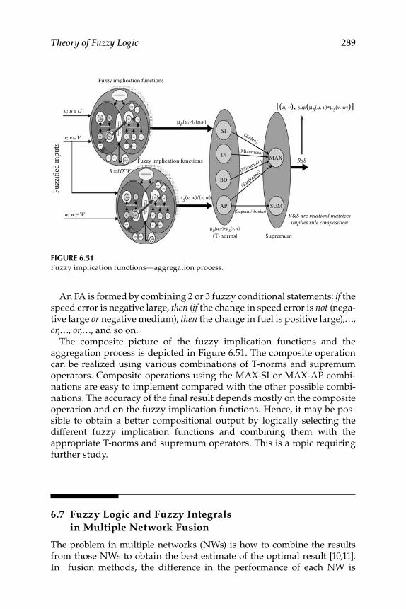
Theory of Fuzzy Logic 289

An FA is formed by combining 2 or 3 fuzzy conditional statements: if the speed error is negative large, then (if the change in speed error is not (nega-tive large or negative medium), then the change in fuel is positive large),…, or,…, or,…, and so on.

The composite picture of the fuzzy implication functions and the aggregation process is depicted in Figure 6.51. The composite operation can be realized using various combinations of T-norms and supremum operators. Composite operations using the MAX-SI or MAX-AP combi-nations are easy to implement compared with the other possible combi-nations. The accuracy of the fi nal result depends mostly on the composite operation and on the fuzzy implication functions. Hence, it may be pos-sible to obtain a better compositional output by logically selecting the different fuzzy implication functions and combining them with the appropriate T-norms and supremum operators. This is a topic requiring further study.

6.7 Fuzzy Logic and Fuzzy Integrals

in Multiple Network Fusion

The problem in multiple networks (NWs) is how to combine the results from those NWs to obtain the best estimate of the optimal result [10,11]. In fusion methods, the difference in the performance of each NW is

SI

DI

BD

AP SUM

MAX RoSFuzzy implication functions

Fuzzy implication functions

Fuzz

ified

inpu

ts

(T-norms) Supremum

R&S are relationl matricesimplies rule composition

(Zadeh)

(Mizumoto)

(Mizumoto)

(Kaufmann)

(Sugeno/Kosko)

u; u ∈U

v; v ∈V

w; w ∈W

R = UXW

μR(u,v)/(u,v)

μS(v,w)/(v,w)

μR(u,v)*μS(v,w)

[(u, v), sup(μR(u, v)*μS(v, w))]

FIGURE 6.51Fuzzy implication functions—aggregation process.

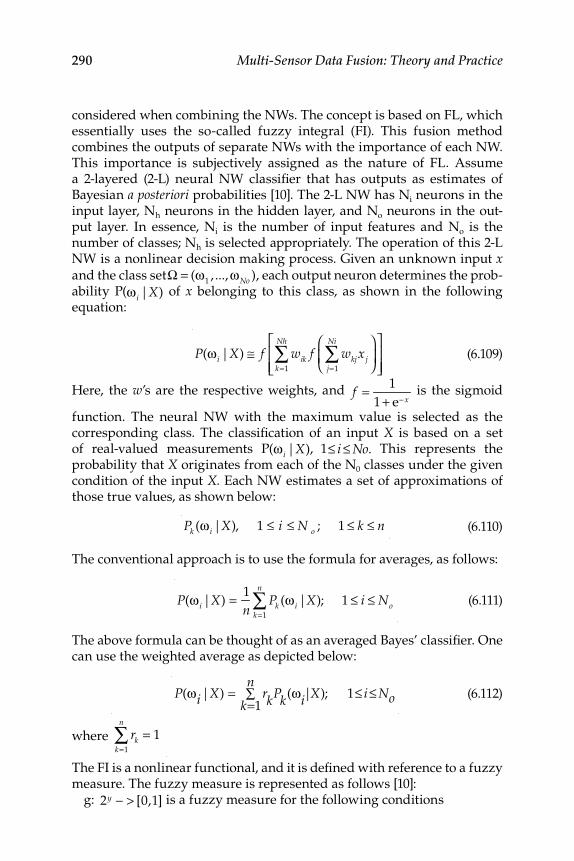
290 Multi-Sensor Data Fusion: Theory and Practice

considered when combining the NWs. The concept is based on FL, which essentially uses the so-called fuzzy integral (FI). This fusion method combines the outputs of separate NWs with the importance of each NW. This importance is subjectively assigned as the nature of FL. Assume a 2- layered (2-L) neural NW classifi er that has outputs as estimates of Bayesian a posteriori probabilities [10]. The 2-L NW has Ni neurons in the input layer, Nh neurons in the hidden layer, and No neurons in the out-put layer. In essence, Ni is the number of input features and No is the number of classes; Nh is selected appropriately. The operation of this 2-L NW is a nonlinear decision making process. Given an unknown input x

and the class setΩ = (ω1, ...,ωNo ), each output neuron determines the prob-

ability P(ω i |X) of x belonging to this class, as shown in the following equation:

P(ω i |X) ≅ f wik f wkjxjj=1

Ni

∑⎛

⎝⎜⎞

⎠⎟k=1

Nh

∑⎡

⎣⎢⎢

⎤

⎦⎥⎥ (6.109)

Here, the w’s are the respective weights, and f = 1

1 + e− x is the sigmoid

function. The neural NW with the maximum value is selected as the corresponding class. The classifi cation of an input X is based on a set of real-valued measurements P(ω i |X), 1≤ i ≤ No. This represents the probability that X originates from each of the N0 classes under the given condition of the input X. Each NW estimates a set of approximations of those true values, as shown below:

Pk (ω i|X), 1 ≤ i ≤ N o ; 1 ≤ k ≤ n (6.110)

The conventional approach is to use the formula for averages, as follows:

P(ω i|X) =

1

nPk (ω i|X); 1 ≤ i ≤ No

k=1

n

∑ (6.111)

The above formula can be thought of as an averaged Bayes’ classifi er. One can use the weighted average as depicted below:

P(ωi|X) = rkPk(ωi|X); 1≤ i ≤ Nok=1

n∑ (6.112)

where

rk = 1

k=1

n

∑The FI is a nonlinear functional, and it is defi ned with reference to a fuzzy measure. The fuzzy measure is represented as follows [10]:

g: 2y − > [0,1] is a fuzzy measure for the following conditions

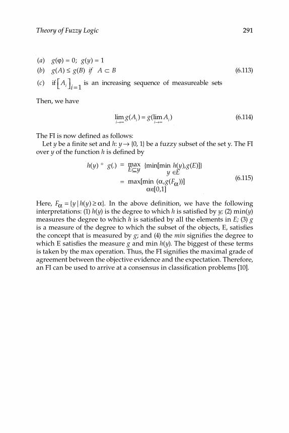
Theory of Fuzzy Logic 291

(a) g(ϕ) = 0; g(y) = 1

(b) g(A) ≤ g(B) if A ⊂ B

(c) if Ai⎡⎣ ⎤⎦ i = 1 is an increasing sequence of measureable sets

(6.113)

Then, we have

limi→∞

g(Ai ) = g(limi→∞

Ai ) (6.114)

The FI is now defi ned as follows:Let y be a fi nite set and h: y → {0, 1} be a fuzzy subset of the set y. The FI

over y of the function h is defi ned by

h(y) ° g(.) = maxE⊆y {min[min h(y),g(E)]}

y ∈E= max[min (α,g(Fα))]

α∈[0,1]

(6.115)

Here, Fα = {y|h(y) ≥ α}. In the above defi nition, we have the following interpretations: (1) h(y) is the degree to which h is satisfi ed by y; (2) min(y) measures the degree to which h is satisfi ed by all the elements in E; (3) g is a measure of the degree to which the subset of the objects, E, satisfi es the concept that is measured by g; and (4) the min signifi es the degree to which E satisfi es the measure g and min h(y). The biggest of these terms is taken by the max operation. Thus, the FI signifi es the maximal grade of agreement between the objective evidence and the expectation. Therefore, an FI can be used to arrive at a consensus in classifi cation problems [10].

293

7 Decision Fusion

The objective of decision fusion is to arrive at one fi nal decision or action from an entire surveillance volume at any instant of time using outputs from different levels—for example, level 1, object refi nement (OR), and level 2, situation refi nement (SR)—of any multisensor data fusion (MSDF) system, especially in defense systems (see the JDL model in Section 2.1). The procedure is also applicable to other civilian data fusion (DF) systems.

7.1 Symbol- or Decision-Level Fusion

Symbol-level fusion (used synonymously for decision fusion) repre-sents high-level information (higher than both the kinematic-level and image-level fusion processes), wherein the symbol represents a deci-sion. A symbol can represent an input in the form of a decision; fusion describes both a logical and a statistical inference. In the case of sym-bolic data, inference methods from artifi cial intelligence can be used as computational mechanisms, such as fuzzy logic (FL), since the fusion of symbolic information would require reasoning and inference in the presence of uncertainty.

There are generally three domains of objects which can provide information [12]: (1) the concrete domain of physical objects with physi-cal characteristics, physical states, activities and tangible entities (e.g., an aircraft or a robot); (2) the abstract domain—the “mind-thought” process, which covers the domain of the mind of all living beings and all intan-gible entities; and (3) the symbol domain—where the characteristics of concrete and abstract entities are transformed into representations of common systems of symbols (for communication and possible dynamic interactions). Interestingly, all three domains can be found in multiple interacting systems, for example, a group of mobile robots, which com-plicates decision making in terms of coordination and team autonomy. The sensing and data processing part of the robotic system builds the world model of the robot’s environment (the robot’s “mind”—in fact

294 Multi-Sensor Data Fusion: Theory and Practice

the “mind” constructs an internal model of the outside world), which contains the physical objects and symbols (e.g., sign boards, traffi c signs, and so on). The decision process consists of (1) decoding information, interpretations, and associations by using previous experiences; and (2) perception of interpreted and associated sensory impressions that would lead to meaning (this is also called new information ). The sensing process precedes the decision process, which is followed by the behav-ioral process. The sensing and decision processes together are called the information process cycle, with appropriate feedback where applicable. According to one theory of intelligence [13,14], the unknowable external world, noumena, is distinguished from the perceptual stimuli result-ing from that world, phenomena. The noumena, which are not directly knowable (e.g., fi re, river), are the sources of the perceptual stimuli. Many worldly phenomena represent a partial projection (a small cross-section, features, and so on) of noumena. Humans organize perceived phenomena into schemata, which represent individual phenomena and abstractions. This is a systematic procedure involving some regularity or pattern in these phenomena. For example, the properties measured by the sensors are the phenomena, and the vector of these properties is a form of schemata. The schemata, also used in the theory of genetic algorithms, can include temporal sequences and images. The reasoning process about the world requires an abstraction from the phenomena: (1) categories of objects, (2) relations between objects, (3) actions, and (4) events, many of which can be represented by labels, that is, symbols. Thus, a symbol is a sign that represents a thing.

The symbol states of information consists of (1) a set of symbolic representation-like text and sound in a language and pictures, and (2) information products and outcomes such as documents and speeches [12]. This symbol-level information can be used for encoding and decod-ing our thought processes. Symbols—such as signs, letters, sounds in and of languages, pictures, maps, and objects representing something—can form information products and outcomes such as data, messages, facts, reports, books, intelligent information, speeches, models, simulation out-puts, computer programs, media products, fi nancial products (e.g., coins and currency notes), ethnic and religious symbols, national and politi-cal symbols (e.g., emblems, fl ags, and election, party, or union symbols or logos). In effect, information process refi nement (PR) starts from the signs, progresses to data to symbols, facts, and ideas, and then to knowledge and wisdom. Symbols represent input in the form of a decision, where as fusion describes a logical and statistical inference. The signifi cant advan-tage of symbol-level fusion is an increase in the truth value. This type of fusion can also be considered decision fusion.

The main decision-level fusion approaches are identity- and knowledge-based methods [15,16]. In the identity-based approach, maximum a

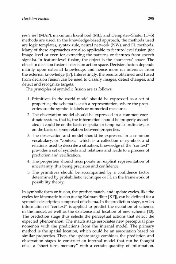
Decision Fusion 295

posteriori (MAP), maximum likelihood (ML), and Dempster–Shafer (D–S) methods are used. In the knowledge-based approach, the methods used are logic templates, syntax rule, neural network (NW), and FL methods. Many of these approaches are also applicable to feature-level fusion (for image level or even for extracting the patterns or features from speech signals). In feature-level fusion, the object is the characters’ space. The object in decision fusion is decision action space. Decision fusion depends mainly upon external knowledge, and hence more on inference from the external knowledge [17]. Interestingly, the results obtained and fused from decision fusion can be used to classify images, detect changes, and detect and recognize targets.

The principles of symbolic fusion are as follows:

1. Primitives in the world model should be expressed as a set of properties; the schema is such a representation, where the prop-erties are the symbolic labels or numerical measures.

2. The observation model should be expressed in a common coor-dinate system, that is, the information should be properly associ-ated; it could be on the basis of spatial or temporal coordinates, or on the basis of some relation between properties.

3. The observation and model should be expressed in a common vocabulary, or “context,” which is a collection of symbols and relations used to describe a situation; knowledge of the “context” provides a set of symbols and relations and leads to a process of prediction and verifi cation.

4. The properties should incorporate an explicit representation of uncertainty, this being precision and confi dence.

5. The primitives should be accompanied by a confi dence factor determined by probabilistic technique or FL in the framework of possibility theory.

In symbolic form or fusion, the predict, match, and update cycles, like the cycles for kinematic fusion (using Kalman fi lter [KF]), can be defi ned for a symbolic description composed of schema. In the prediction stage, a priori information of “context” is applied to predict the evolution of schemes in the model, as well as the existence and location of new schema [13]. The prediction stage thus selects the perceptual actions that detect the expected phenomenon. The match stage associates new perceptual phe-nomenon with the predictions from the internal model. The primary method is the spatial location, which could be an association based on similar properties. Then, the update stage combines the prediction and observation stages to construct an internal model that can be thought of as a “short term memory” with a certain quantity of information.

296 Multi-Sensor Data Fusion: Theory and Practice

In Chapters 7 and 8, the use of FL is regarded as helping a decision process either in KF or situation assessment (SA).

7.2 Soft Decisions in Kalman Filtering

The KF has been used as one of the most promising algorithms for recur-sive estimation of states of linear and nonlinear systems. The accuracy of the fi lter is based on (1) the accuracy of the mathematical model of the actual dynamic system and measurement device, due to the random uncertainties; and (2) its tuning parameters Q (process noise covariance matrix) and R (measurement noise covariance matrix). In some applica-tions, we may encounter a modeling error, that is, when the true models are not accurately known or they are diffi cult to realize or implement, we have to use approximate representations. Modeling errors are often compensated for by process noise-tuning parameters (of Q ) that are selected on a trial-and-error basis. The fi nal solutions obtained through this approach may not provide optimal fi lter performance. Although there are a few adaptive fi lters that can be used for such purposes, these are computationally very demanding and time varying, especially in the case of the extended KF (EKF).

The gain of a KF determines how much weighting should be given to the present measurement (in fact to the residuals): (1) If the measurement data are highly contaminated with noise, then less weight is automatically assigned to that data, and the fi lter depends on the model of the target (i.e., state propagation, see Equations 2.23 and 2.24); and (2) if the mea-surement data are less noisy, then more weight is assigned to that data, and the estimated state is a combination of state-predicted (through a tar-get model) and observation data. Thus, the KF has an inherent decision- making capability that helps in soft switching between the process model and measurement model (via appropriate weight assignments, Kalman gain, and P , Q , and R ). This decision in soft switching is based on Kalman gain that depends on the relative value of tuning parameters and matrices Q and R .

Measurement noise variance refl ects the noise level in measurement data; higher R (in terms of the norm of the matrix) means the data is very noisy, and vice versa . In cases of very high R , the fi lter does not trust the measurement data, and therefore assigns low weight to the correction part of the state update through Kalman gain (Equation 2.20). This can also be interpreted as that the fi lter relies mostly on the process model. Similarly, for very low R , the fi lter relies mostly on the measurement model. Table 7.1 summarizes the soft decisions in a KF [7].

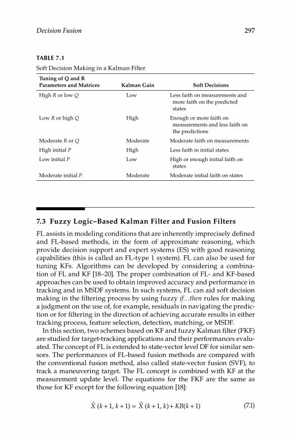
Decision Fusion 297

7.3 Fuzzy Logic–Based Kalman Filter and Fusion Filters

FL assists in modeling conditions that are inherently imprecisely defi ned and FL-based methods, in the form of approximate reasoning, which provide decision support and expert systems (ES) with good reasoning capabilities (this is called an FL-type 1 system ). FL can also be used for tuning KFs. Algorithms can be developed by considering a combina-tion of FL and KF [18–20]. The proper combination of FL- and KF-based approaches can be used to obtain improved accuracy and performance in tracking and in MSDF systems. In such systems, FL can aid soft decision making in the fi ltering process by using fuzzy if…then rules for making a judgment on the use of, for example, residuals in navigating the predic-tion or for fi ltering in the direction of achieving accurate results in either tracking process, feature selection, detection, matching, or MSDF.

In this section, two schemes based on KF and fuzzy Kalman fi lter (FKF) are studied for target-tracking applications and their performances evalu-ated. The concept of FL is extended to state-vector level DF for similar sen-sors. The performances of FL-based fusion methods are compared with the conventional fusion method, also called state-vector fusion (SVF), to track a maneuvering target. The FL concept is combined with KF at the measurement update level. The equations for the FKF are the same as those for KF except for the following equation [18]:

X (k + 1, k + 1) = %X (k + 1, k) + KB(k + 1) (7.1)

TABLE 7.1

Soft Decision Making in a Kalman Filter

Tuning of Q and R

Parameters and Matrices Kalman Gain Soft Decisions

High R or low Q Low Less faith on measurements and

more faith on the predicted

states

Low R or high Q High Enough or more faith on

measurements and less faith on

the predictions

Moderate R or Q Moderate Moderate faith on measurements

High initial P High Less faith in initial states

Low initial P Low High or enough initial faith on

states

Moderate initial P Moderate Moderate initial faith on states

298 Multi-Sensor Data Fusion: Theory and Practice

Here, B(k + 1) is regarded as an output of the FL-based process variable (FLPV) and is generally a nonlinear function of the innovations e of the KF. It is assumed that positions in x – y axes measurements of the target are available. The FLPV vector consists of the modifi ed innovation sequence for x and y axes:

B(k + 1) = [bx(bx (k + 1)by (k + 1)] (7.2)

To determine the FLPV vector, the innovation vector e is fi rst separated into its x and y components, ex and ey. The target motion in each axis is assumed to be independent. The FLPV vector for the x direction is developed and then generalized to include y direction. This vector con-sists of two inputs, ex and &ex, and single output bx(k + 1), where &ex is computed by

&ex =

ex(k + 1) − ex(k){ }T (7.3)

Here, T is the sampling interval in seconds; the expression of Equation 7.3 can be extended to y direction, and even to z direction if required.

7.3.1 Fuzzy Logic–Based Process and Design

FLP is obtained via a fuzzy inference system (FIS); see Figures 6.13 and 6.14. Sections 6.1.4 and 6.1.9 list the steps to build an FIS. The antecedent membership functions that defi ne the fuzzy values for inputs ex and &ex and the membership function for the output bx needed to develop the FLP are shown in Figure 7.1 [20]. The linguistic variables or labels to defi ne membership functions are large negative (LN), medium negative (MN), small negative (SN), zero error (ZE), small positive (SP), medium positive (MP), and large positive (LP). The rules for the inference in FIS are gener-ally created based on the experience and intuition of the domain expert, one such rule being [9,18,20]:

IF ex is LP AND &ex is LP THEN bx is LP (7.4)

Having ex and &ex with large positive values indicates an increase in the innovation sequence at faster rate. Then, the future value of ex (and hence &ex) can be reduced by increasing the present value of bx (≈ Z − H %X) by a large magnitude. This will generate 49 rules to implement FLP. The out-put bx at any instant of time can be computed using (1) the inputs ex and &ex, (2) input membership functions, (3) the 49 rules [9,18,20], (4) FIS, (5) the

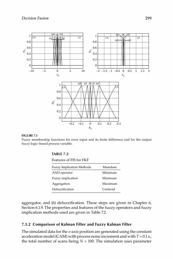
Decision Fusion 299

aggregator, and (6) defuzzifi cation. These steps are given in Chapter 6, Section 6.1.9. The properties and features of the fuzzy operators and fuzzy implication methods used are given in Table 7.2.

7.3.2 Comparison of Kalman Filter and Fuzzy Kalman Filter

The simulated data for the x -axis position are generated using the constant acceleration model (CAM) with process noise increment and with T = 0.1 s.,the total number of scans being N = 100. The simulation uses parameter

-0.2 -0.1 0 0.1 0.2 0.30

0.2

0.4

0.6

0.8

1LN

MN SN ZE SP MPLP

m bx

bx

-10 -5 0 5 100

0.20.4

0.60.8

1 LNMN

SNZE

SPMP

LP

-2 -1.5 -1 -0.5 0 0.5 1 1.5 2

LNMN

SN ZE

MPLP

m ex

m ex

00.20.4

0.60.8

1

ex ex

SP

FIGURE 7.1 Fuzzy membership functions for error input and its fi nite difference and for the output

fuzzy logic–based process variable.

TABLE 7.2

Features of FIS for FKF

Fuzzy Implication Methods Mamdani

AND operator Minimum

Fuzzy implication Minimum

Aggregation Maximum

Defuzzifi cation Centroid

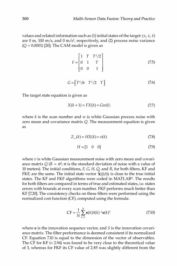
300 Multi-Sensor Data Fusion: Theory and Practice

values and related information such as (1) initial states of the target: (x, &x, &&x) are 0 m, 100 m/s, and 0 m/s 2 , respectively, and (2) process noise variance ( Q = 0.0001) [20]. The CAM model is given as

F =1 T T 2/2

0 1 T

0 0 1

⎡

⎣

⎢⎢⎢

⎤

⎦

⎥⎥⎥

(7.5)

G = T 3/6 T 2/2 T⎡⎣ ⎤⎦

(7.6)

The target state equation is given as

X(k + 1) = FX(k) + Gw(k) (7.7)

where k is the scan number and w is white Gaussian process noise with zero mean and covariance matrix Q. The measurement equation is given as

Zm(k) = HX(k) + v(k) (7.8)

H = [1 0 0] (7.9)

where v is white Gaussian measurement noise with zero mean and covari-ance matrix Q (R = σ2; σ is the standard deviation of noise with a value of 10 meters). The initial conditions, F, G, H, Q, and R, for both fi lters, KF and FKF, are the same. The initial state vector X(0/0) is close to the true initial states. The KF and FKF algorithms were coded in MATLAB®. The results for both fi lters are compared in terms of true and estimated states, i.e. states errors with bounds at every scan number. FKF performs much better than KF [7,20]. The consistency checks on these fi lters were performed using the normalized cost function (CF), computed using the formula:

CF = 1

Ne(k)S(k)−1

k=1

N

∑ e(k)T

(7.10)

where e is the innovation sequence vector, and S is the innovation covari-ance matrix. The fi lter performance is deemed consistent if its normalized CF. Equation 7.10 is equal to the dimension of the vector of observables. The CF for KF (= 2.94) was found to be very close to the theoretical value of 3, whereas for FKF its CF value of 2.85 was slightly different from the

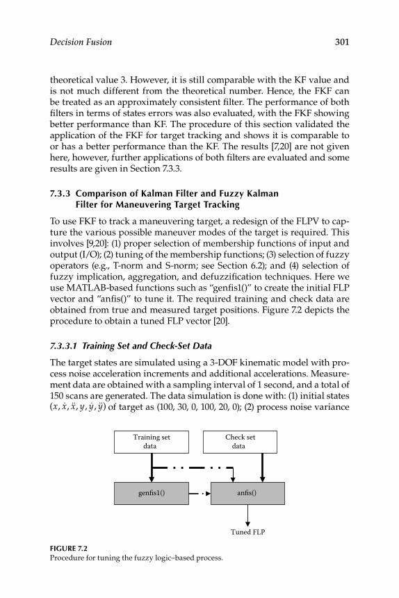
Decision Fusion 301

theoretical value 3. However, it is still comparable with the KF value and is not much different from the theoretical number. Hence, the FKF can be treated as an approximately consistent fi lter. The performance of both fi lters in terms of states errors was also evaluated, with the FKF showing better performance than KF. The procedure of this section validated the application of the FKF for target tracking and shows it is comparable to or has a better performance than the KF. The results [7,20] are not given here, however, further applications of both fi lters are evaluated and some results are given in Section 7.3.3.

7.3.3 Comparison of Kalman Filter and Fuzzy Kalman Filter for Maneuvering Target Tracking

To use FKF to track a maneuvering target, a redesign of the FLPV to cap-ture the various possible maneuver modes of the target is required. This involves [9,20]: (1) proper selection of membership functions of input and output (I/O); (2) tuning of the membership functions; (3) selection of fuzzy operators (e.g., T-norm and S-norm; see Section 6.2); and (4) selection of fuzzy implication, aggregation, and defuzzifi cation techniques. Here we use MATLAB-based functions such as “genfi s1()” to create the initial FLP vector and “anfi s()” to tune it. The required training and check data are obtained from true and measured target positions. Figure 7.2 depicts the procedure to obtain a tuned FLP vector [20].

7.3.3.1 Training Set and Check-Set Data

The target states are simulated using a 3-DOF kinematic model with pro-cess noise acceleration increments and additional accelerations. Measure-ment data are obtained with a sampling interval of 1 second, and a total of 150 scans are generated. The data simulation is done with: (1) initial states (x, &x, &&x, y, &y, &&y) of target as (100, 30, 0, 100, 20, 0); (2) process noise variance

FIGURE 7.2 Procedure for tuning the fuzzy logic–based process.

Training setdata

Check setdata

genfis1() anfis()

Tuned FLP

302 Multi-Sensor Data Fusion: Theory and Practice

Q = 0.1 (it is assumed that Qxx = Qyy = Q); and (3) measurement noise variance ( R = 25). We also assume that Rxx = Ryy = R. The target has an additional acceleration of (xacc, yacc) at scans 25 and 100 and an acceleration of (−xacc, −yacc) at scans 50 and 75. Data simulation is carried out with process noise vector w (a 2 × 1 vector) modifi ed to include these additional accelerations at the specifi ed scan points, in order to induce a specifi c maneuver [9,20]:

w(1) = guass()× Qxx + xacc

w(2) = guass() × Qyy + yacc

⎫⎬⎪

⎭⎪

(7.11)

w(1) = guass()× Qxx − xacc

w(2) = guass() × Qyy − yacc

⎫⎬⎪

⎭⎪

(7.12)

At the other scan points, the vector w is simply defi ned without these additional accelerations terms. Acceleration xacc = −9 × 9.8 m/s2 and yacc = 9 × 9.8 m/s2 are used in the above equations and the function gauss() is used to generate Gaussian random numbers with mean 0 and variance 1. First, the initial FLPV is created for the x axis and tuned using inputs ux

1 , ux2 , and output ox is obtained using:

ux1 (k) = zx (k) − x(k) (7.13)

ux

2 (k) =ux

1 (k) − ux1 (k − 1)

T (7.14)

outputx(k) = mux

1 (k)

(7.15)

Here, x and zx are the true and measured target x position, respectively. m is the unknown parameter and is 2 for the present case. The fi rst half of the total simulated data is taken for training and the remaining half is taken as the check-set data. The same procedure is followed to get the tuned FLPV for the y axis; then the trained FLP vector is plugged in to the FKF and its performance is compared with the KF for the two cases discussed next.

7.3.3.2 Mild and Evasive Maneuver Data

The mild maneuver (MM) data are generated with minor modifi cations in the acceleration injection points, with a total of 17 scans generated. Accelerations are injected at scans 8 (xacc = 6 m/s2 and yacc = −6 m/s2) and 15 (xacc = −6 m/s2 and yacc = 6 m/s2) only [20]. The evasive maneuver (EM)

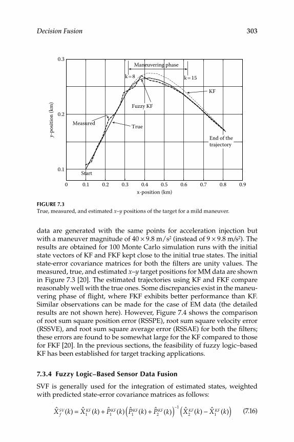
Decision Fusion 303

data are generated with the same points for acceleration injection but with a maneuver magnitude of 40 × 9.8 m/s2 (instead of 9 × 9.8 m/s2). The results are obtained for 100 Monte Carlo simulation runs with the initial state vectors of KF and FKF kept close to the initial true states. The initial state-error covariance matrices for both the fi lters are unity values. The measured, true, and estimated x – y target positions for MM data are shown in Figure 7.3 [20]. The estimated trajectories using KF and FKF compare reasonably well with the true ones. Some discrepancies exist in the maneu-vering phase of fl ight, where FKF exhibits better performance than KF. Similar observations can be made for the case of EM data (the detailed results are not shown here). However, Figure 7.4 shows the comparison of root sum square position error (RSSPE), root sum square velocity error (RSSVE), and root sum square average error (RSSAE) for both the fi lters; these errors are found to be somewhat large for the KF compared to those for FKF [20]. In the previous sections, the feasibility of fuzzy logic–based KF has been established for target tracking applications.

7.3.4 Fuzzy Logic–Based Sensor Data Fusion

SVF is generally used for the integration of estimated states, weighted with predicted state-error covariance matrices as follows:

X f

SV(k) = X1KF (k) + P

1KF(k) P

1KF(k) + P

2KF(k)( )−1

X2KF(k) − X

1KF (k)( )

(7.16)

0 0.1 0.2 0.3 0.4 0.5 0.6 0.7 0.8 0.9

0.1

0.2

0.3

x-position (km)

y-po

sitio

n (k

m)

Start

End of thetrajectory

KF

Measured True

Maneuvering phase

k = 8 k = 15

Fuzzy KF

FIGURE 7.3 True, measured, and estimated x – y positions of the target for a mild maneuver.

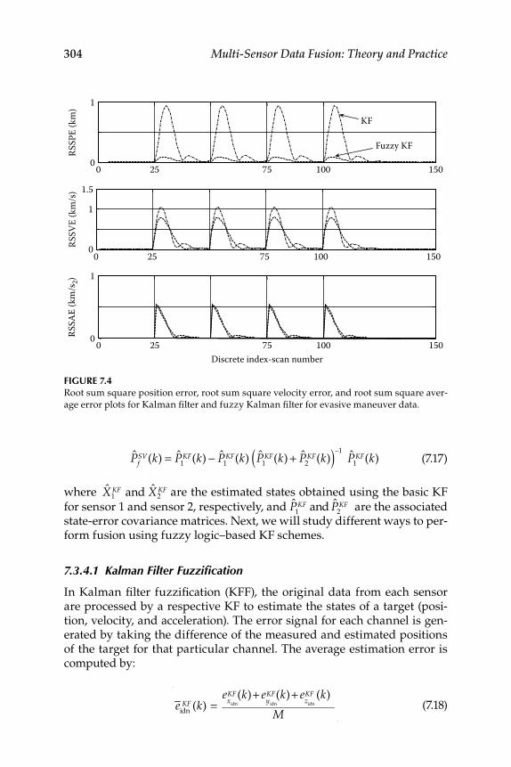
304 Multi-Sensor Data Fusion: Theory and Practice

PfSV(k) = P

1KF(k) − P

1KF(k) P

1KF(k) + P

2KF(k)( )−1

P1KF(k) (7.17)

where X1KF and X2

KF are the estimated states obtained using the basic KF

for sensor 1 and sensor 2, respectively, and P1KF and P

2KF are the associated

state-error covariance matrices. Next, we will study different ways to per-form fusion using fuzzy logic–based KF schemes.

7.3.4.1 Kalman Filter Fuzzifi cation

In Kalman fi lter fuzzifi cation (KFF), the original data from each sensor are processed by a respective KF to estimate the states of a target (posi-tion, velocity, and acceleration). The error signal for each channel is gen-erated by taking the difference of the measured and estimated positions of the target for that particular channel. The average estimation error is computed by:

e

idnKF (k) =

exidn

KF(k)+ eyidn

KF(k)+ ezidn

KF (k)

M (7.18)

0 25 75 100 150

0 25 75 100 150

0 25 75 100 150

0

1

RSSP

E (k

m)

1

0

1.5

RSSV

E (k

m/s

)

0

1

RSSA

E (k

m/s

2)

Discrete index-scan number

KF

Fuzzy KF

FIGURE 7.4 Root sum square position error, root sum square velocity error, and root sum square aver-

age error plots for Kalman fi lter and fuzzy Kalman fi lter for evasive maneuver data.

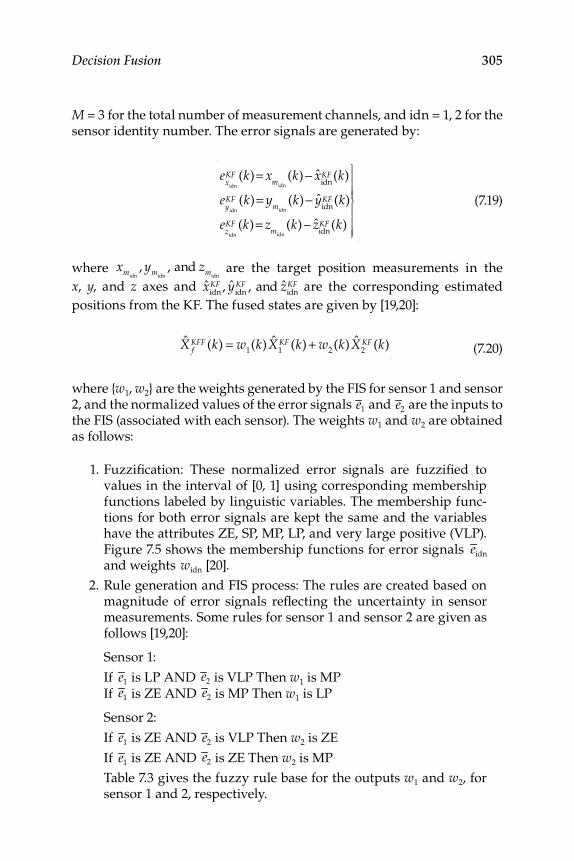
Decision Fusion 305

M = 3 for the total number of measurement channels, and idn = 1, 2 for the sensor identity number. The error signals are generated by:

exidn

KF (k)= xmidn

(k)− xidnKF (k)

eyidn

KF (k)= ymidn

(k)− yidnKF (k)

ezidn

KF (k)= zmidn

(k)− zidnKF (k)

⎫

⎬

⎪⎪⎪⎪

⎭

⎪⎪⎪⎪

(7.19)

where xmidn, ymidn

, and zmidn are the target position measurements in the

x , y , and z axes and xidnKF , y

idnKF , and z

idnKF are the corresponding estimated

positions from the KF. The fused states are given by [19,20]:

X f

KFF (k) = w1(k)X

1KF (k) + w

2(k)X

2KF (k)

(7.20)

where {w1, w2} are the weights generated by the FIS for sensor 1 and sensor 2, and the normalized values of the error signals e1 and e2 are the inputs to the FIS (associated with each sensor). The weights w1 and w2 are obtained as follows:

1. Fuzzifi cation: These normalized error signals are fuzzifi ed to values in the interval of [0, 1] using corresponding membership functions labeled by linguistic variables. The membership func-tions for both error signals are kept the same and the variables have the attributes ZE, SP, MP, LP, and very large positive (VLP). Figure 7.5 shows the membership functions for error signals eidn and weights widn [20].

2. Rule generation and FIS process: The rules are created based on magnitude of error signals refl ecting the uncertainty in sensor measurements. Some rules for sensor 1 and sensor 2 are given as follows [19,20]:

Sensor 1:

If e1 is LP AND e2 is VLP Then w1 is MP If e1 is ZE AND e2 is MP Then w1 is LP

Sensor 2:

If e1 is ZE AND e2 is VLP Then w2 is ZE

If e1 is ZE AND e2 is ZE Then w2 is MP

Table 7.3 gives the fuzzy rule base for the outputs w1 and w2, for sensor 1 and 2, respectively.

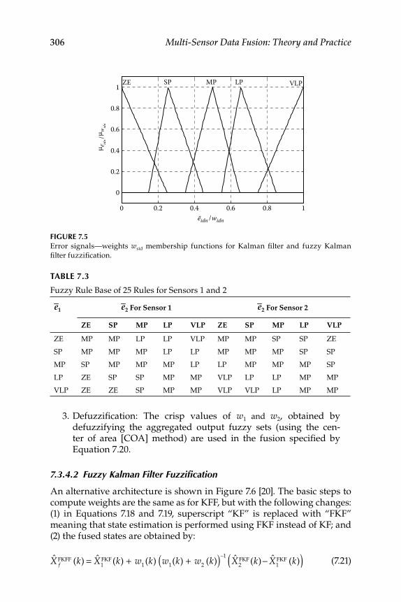
306 Multi-Sensor Data Fusion: Theory and Practice

3. Defuzzifi cation: The crisp values of w1 and w2, obtained by defuzzifying the aggregated output fuzzy sets (using the cen-ter of area [COA] method) are used in the fusion specifi ed by Equation 7.20.

7.3.4.2 Fuzzy Kalman Filter Fuzzifi cation

An alternative architecture is shown in Figure 7.6 [20]. The basic steps to compute weights are the same as for KFF, but with the following changes: (1) in Equations 7.18 and 7.19, superscript “KF” is replaced with “FKF” meaning that state estimation is performed using FKF instead of KF; and (2) the fused states are obtained by:

X f

FKFF (k) = X1FKF (k) + w

1(k) w

1(k) + w

2(k)( )−1

X2FKF (k)− X

1FKF (k)( )

(7.21)

TABLE 7.3

Fuzzy Rule Base of 25 Rules for Sensors 1 and 2

e1 e2 For Sensor 1 e2 For Sensor 2

ZE SP MP LP VLP ZE SP MP LP VLP

ZE MP MP LP LP VLP MP MP SP SP ZE

SP MP MP MP LP LP MP MP MP SP SP

MP SP MP MP MP LP LP MP MP MP SP

LP ZE SP SP MP MP VLP LP LP MP MP

VLP ZE ZE SP MP MP VLP VLP LP MP MP

FIGURE 7.5 Error signals—weights wsid membership functions for Kalman fi lter and fuzzy Kalman

fi lter fuzzifi cation.

m eid

nm w

idn

/

eidn widn/0 0.2 0.4 0.6 0.8 1

0

0.2

0.4

0.6

0.8

1 ZE SP MP LP VLP

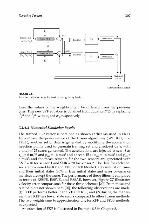
Decision Fusion 307

Here the values of the weights might be different from the previous ones. This new SVF equation is obtained from Equation 7.16 by replacing

P1KF and P

2KF with w1 and w2, respectively.

7.3.4.3 Numerical Simulation Results

The trained FLP vector is obtained as shown earlier (as used in FKF). To compare the performance of the fusion algorithms (SVF, KFF, and FKFF), another set of data is generated by modifying the acceleration injection points used to generate training set and check-set data, with a total of 25 scans generated. The accelerations are injected at scan 8 as xacc = 6 m/s2 and yacc = −6 m/s2 and at scan 15 as xacc = −6 m/s2 and yacc = 6 m/s2, and the measurements for the two sensors are generated with SNR = 10 for sensor 1 and SNR = 20 for sensor 2. The data for each sen-sor are processed by KF and FKF for 100 Monte Carlo simulation runs, and their initial states (80% of true initial state) and error covariance matrices are kept the same. The performance of these fi lters is compared in terms of RSSPE, RSSVE, and RSSAE, however, Figure 7.7 illustrates velocity error comparisons for these three schemes [20]. From these and related plots not shown here [20], the following observations are made: (1) FKFF performs better than SVF and KFF; and (2) during the maneu-ver, the FKFF has fewer state errors compared to other fusion methods. The two weights sum to approximately one for KFF and FKFF methods, as expected.

An extension of FKF is illustrated in Example 8.3 in Chapter 8.

FIGURE 7.6 An alternative scheme for fusion using fuzzy logic.

FuzzifierFIS Defuzzifier

Sensor No. 1 (xm1

, ym1, zm1)

(xm2, ym2

, zm2) Sensor No. 2

Fuzzy KF 1

Fuzzy KF 2

Q

R1

R2

+_

+_

Fuzzifier FIS Defuzzifier

WeightedFusion

e1FKFF w1

w2

State vector fusion output

e2FKFF

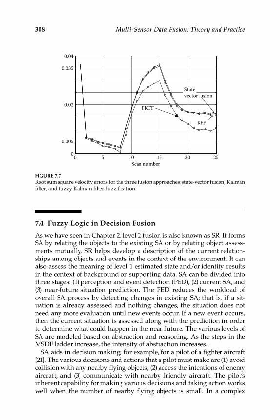
308 Multi-Sensor Data Fusion: Theory and Practice

7.4 Fuzzy Logic in Decision Fusion

As we have seen in Chapter 2, level 2 fusion is also known as SR. It forms SA by relating the objects to the existing SA or by relating object assess-ments mutually. SR helps develop a description of the current relation-ships among objects and events in the context of the environment. It can also assess the meaning of level 1 estimated state and/or identity results in the context of background or supporting data. SA can be divided into three stages: (1) perception and event detection (PED), (2) current SA, and (3) near-future situation prediction. The PED reduces the workload of overall SA process by detecting changes in existing SA; that is, if a sit-uation is already assessed and nothing changes, the situation does not need any more evaluation until new events occur. If a new event occurs, then the current situation is assessed along with the prediction in order to determine what could happen in the near future. The various levels of SA are modeled based on abstraction and reasoning. As the steps in the MSDF ladder increase, the intensity of abstraction increases.

SA aids in decision making; for example, for a pilot of a fi ghter aircraft [21]. The various decisions and actions that a pilot must make are (1) avoid collision with any nearby fl ying objects; (2) access the intentions of enemy aircraft; and (3) communicate with nearby friendly aircraft. The pilot’s inherent capability for making various decisions and taking action works well when the number of nearby fl ying objects is small. In a complex

FIGURE 7.7 Root sum square velocity errors for the three fusion approaches: state-vector fusion, Kalman

fi lter, and fuzzy Kalman fi lter fuzzifi cation.

0 5 10 15 20 250

0.005

0.02

0.035

0.04

Scan number

FKFF

KFF

Statevector fusion

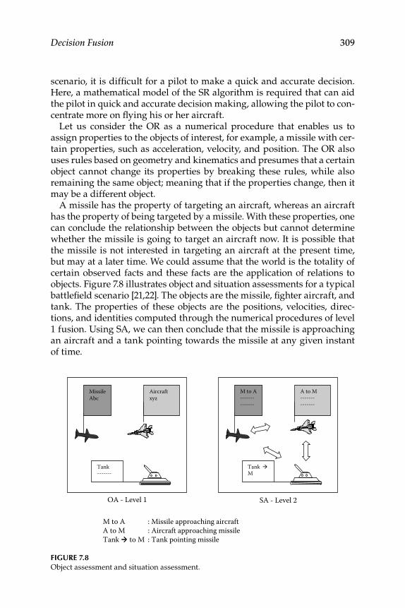
Decision Fusion 309

scenario, it is diffi cult for a pilot to make a quick and accurate decision. Here, a mathematical model of the SR algorithm is required that can aid the pilot in quick and accurate decision making, allowing the pilot to con-centrate more on fl ying his or her aircraft.

Let us consider the OR as a numerical procedure that enables us to assign properties to the objects of interest, for example, a missile with cer-tain properties, such as acceleration, velocity, and position. The OR also uses rules based on geometry and kinematics and presumes that a certain object cannot change its properties by breaking these rules, while also remaining the same object; meaning that if the properties change, then it may be a different object.

A missile has the property of targeting an aircraft, whereas an aircraft has the property of being targeted by a missile. With these properties, one can conclude the relationship between the objects but cannot determine whether the missile is going to target an aircraft now. It is possible that the missile is not interested in targeting an aircraft at the present time, but may at a later time. We could assume that the world is the totality of certain observed facts and these facts are the application of relations to objects. Figure 7.8 illustrates object and situation assessments for a typical battlefi eld scenario [21,22]. The objects are the missile, fi ghter aircraft, and tank. The properties of these objects are the positions, velocities, direc-tions, and identities computed through the numerical procedures of level 1 fusion. Using SA, we can then conclude that the missile is approaching an aircraft and a tank pointing towards the missile at any given instant of time.

FIGURE 7.8 Object assessment and situation assessment.

MissileAbc

Aircraftxyz

Tank -------

M to A ------- -------

A to M ------- -------

Tank M

OA - Level 1 SA - Level 2

M to A : Missile approaching aircraftA to M : Aircraft approaching missileTank to M : Tank pointing missile

310 Multi-Sensor Data Fusion: Theory and Practice

7.4.1 Methods Available to Perform Situation Assessments

The most commonly used techniques in SA systems are high-level classifi -cation methods; the basic requirement is that they should be able to handle uncertainty with an ease in modeling situations. The common methods for assessing situations are (1) artifi cial neural networks (ANN)s—an ANN would have been trained in some situations; then it would be given the data of the current situation, which might have just occurred. The ANN predicts the situation, and if there is a close match, further decisions are made, and so on; (2) forward-chain ES (FCES; classical); (3) Bayesian NW (BNW), also called belief NW (more appropriate for D–S networks; causal net or inference net); (4) FL—FL/FMF/FIS; and (5) hybrid methods—FL and BNW, ANN, FL, and so on. An ANN can easily recognize situations by learning from training data. The NW must be suffi ciently trained; a lack of suffi cient training data is generally a problem. The FCES requires modeling by an expert and cannot update its knowledge automatically (i.e., it cannot adapt itself from the data), as the system contains only the knowledge of its designer.

BNW can be modeled as an ES and is also able to update beliefs (prob-abilities for BNW and “masses” for D–S methods). It has the ability to investigate hypotheses of the future. To make the system handy, the nodes in the BNW are often discrete and an expert can easily enter estimates of the probabilities for one situation leading to another. This will lead to a “quite good” NW. However, the system is diffi cult to use in real time. Also, BNW needs continuous input data, that is, the data must be classi-fi ed fi rst. The FLES can represent human knowledge and experience in the form of fuzzy rules. These rules can be tuned adaptively or new rules can be created dynamically using sets of I/O data and ANN. This learning method generates optimal fuzzy inference (FI engine of knowledge base) rapidly and with good accuracy as required for time-critical missions. The DF systems produced through partially processed sensory informa-tion and intelligence would have uncertain, incomplete and inaccurate information due to limited sensor capabilities. The FL can handle this for tasks such as (1) SA and decision making through modeling the entity, and (2) models and the associated fuzzy sets (and possibility theory). Hybrid methods utilize the FL approach to classify the continuous input that goes to BNW as discrete input and make the net continuous.

7.4.2 Comparison between Bayesian Network and Fuzzy Logic

Using FL, numerical data can be classifi ed into fuzzy sets of discrete vari-ables. In the classifi cation of numerical data that measures the temperature of a certain material, a normal practice is to assign a grade to the member-ship function, that is, very cold, quite hot, and so on. The problem arises when assigning a grade to temperatures such as 19° and 21°C; the difference

Decision Fusion 311

between the temperatures is not very big, but when classifi ed using hard boundaries, 19°C is treated as cold and 21°C is treated as hot. Trying to model a system using hard boundaries could result in erroneous outputs. Classifi cation can be more precise using fuzzy boundaries. A temperature of 19°C could be classifi ed as cold with a membership value of 0.6 and as hot with a membership value of 0.4. In a similar manner, a temperature of 21°C can be classifi ed as both hot and cold. The importance of fuzzy clas-sifi cation becomes more pronounced when dealing with noisy signals.

7.4.2.1 Situation Assessment Using Fuzzy Logic

When the level of uncertainties increases, situation assessment requires exact reasoning with an upward climb in the DF levels. Using only numer-ical procedures, it is very hard to model the uncertainties so that situa-tions can be assessed as accurately as possible. An application of FL at the higher levels of DF could be a good choice for precise decision making. If one of the outputs of SA is “Aircraft is nonfriendly and targeting tank,” then this event can be interpreted as if the situation assessor makes the decision that “Aircraft is nonfriendly and targeting tank.” Fusion comes into the picture when there is more than one such decision for the same object of interest seen by multiple sensors of different types and accura-cies. The different accuracy levels of each sensor dictate different confi -dence levels while making decisions. To have an accurate decision, it is essential to fuse the decisions (outputs form situation assessor) using the FL approach. This is a decision fusion paradigm and not a direct DF.

Consider a scenario of an unknown aircraft seen by two sensors of dif-ferent types. The fi rst sensor provides identity information and the second sensor measures the direction of the moving aircraft. The goal of FLSA is to make a decision about whether the behavior of the unknown aircraft is hostile or friendly [21,22]. The two inputs are “direction” and “iden-tity” and the single output is “behavior” in FIS, i.e., the situation assessor. The inputs are fuzzifi ed using corresponding membership functions. The input direction and identity have two membership functions, each with linguistic labels {departing, approaching} and {friend, foe}, respectively, and the output has membership functions with linguistic labels {friendly, hostile}. Inputs are aggregated using following inference rules [21–23]:

Rule 1: IF aircraft is departing OR identity is friend THEN behavior is friendly

Rule 2: IF aircraft is approaching OR identity is foe THEN behavior is hostile

In the FL “AND” is min(A, B) and OR is max(A, B), with A and B as two fuzzy sets representing input direction and identity, respectively. There

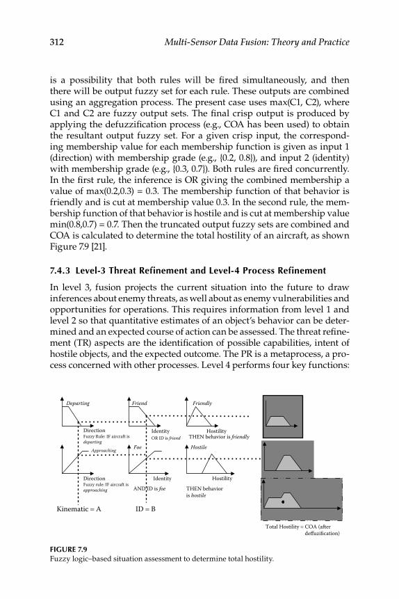
312 Multi-Sensor Data Fusion: Theory and Practice

is a possibility that both rules will be fi red simultaneously, and then there will be output fuzzy set for each rule. These outputs are combined using an aggregation process. The present case uses max(C1, C2), where C1 and C2 are fuzzy output sets. The fi nal crisp output is produced by applying the defuzzifi cation process (e.g., COA has been used) to obtain the resultant output fuzzy set. For a given crisp input, the correspond-ing membership value for each membership function is given as input 1 (direction) with membership grade (e.g., {0.2, 0.8}), and input 2 (identity) with membership grade (e.g., {0.3, 0.7}). Both rules are fi red concurrently. In the fi rst rule, the inference is OR giving the combined membership a value of max(0.2,0.3) = 0.3. The membership function of that behavior is friendly and is cut at membership value 0.3. In the second rule, the mem-bership function of that behavior is hostile and is cut at membership value min(0.8,0.7) = 0.7. Then the truncated output fuzzy sets are combined and COA is calculated to determine the total hostility of an aircraft, as shown Figure 7.9 [21].

7.4.3 Level-3 Threat Refinement and Level-4 Process Refinement

In level 3, fusion projects the current situation into the future to draw inferences about enemy threats, as well about as enemy vulnerabilities and opportunities for operations. This requires information from level 1 and level 2 so that quantitative estimates of an object’s behavior can be deter-mined and an expected course of action can be assessed. The threat refi ne-ment (TR) aspects are the identifi cation of possible capabilities, intent of hostile objects, and the expected outcome. The PR is a metaprocess, a pro-cess concerned with other processes. Level 4 performs four key functions:

FIGURE 7.9 Fuzzy logic–based situation assessment to determine total hostility.

Departing Friend Friendly

Approaching Foe Hostile

Direction

Direction

Identity

Identity

Hostility

Hostility

Kinematic = A ID = B

Fuzzy Rule: IF aircraft isdeparting

OR ID is friend THEN behavior is friendly

Fuzzy rule: IF aircraft isapproaching AND ID is foe THEN behavior

is hostile

Total Hostility = COA (after deffuzification)

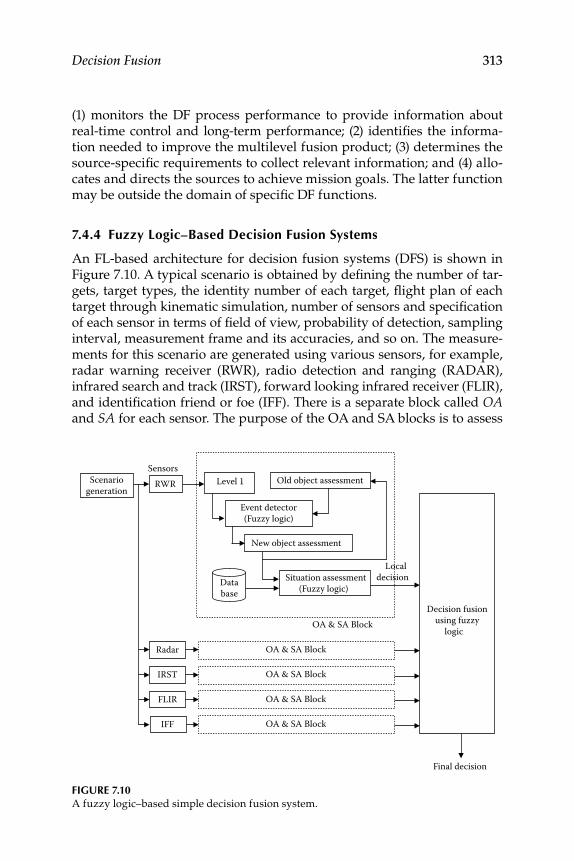
Decision Fusion 313

(1) monitors the DF process performance to provide information about real-time control and long-term performance; (2) identifi es the informa-tion needed to improve the multilevel fusion product; (3) determines the source-specifi c requirements to collect relevant information; and (4) allo-cates and directs the sources to achieve mission goals. The latter function may be outside the domain of specifi c DF functions.

7.4.4 Fuzzy Logic–Based Decision Fusion Systems

An FL-based architecture for decision fusion systems (DFS) is shown in Figure 7.10. A typical scenario is obtained by defi ning the number of tar-gets, target types, the identity number of each target, fl ight plan of each target through kinematic simulation, number of sensors and specifi cation of each sensor in terms of fi eld of view, probability of detection, sampling interval, measurement frame and its accuracies, and so on. The measure-ments for this scenario are generated using various sensors, for example, radar warning receiver (RWR), radio detection and ranging (RADAR), infrared search and track (IRST), forward looking infrared receiver (FLIR), and identifi cation friend or foe (IFF). There is a separate block called OA and SA for each sensor. The purpose of the OA and SA blocks is to assess

FIGURE 7.10 A fuzzy logic–based simple decision fusion system.

Scenariogeneration

RWR

Radar

IRST

FLIR

IFF

Database

New object assessment

Event detector(Fuzzy logic)

Level 1 Old object assessment

Situation assessment(Fuzzy logic)

Decision fusionusing fuzzy

logic OA & SA Block

OA & SA Block

OA & SA Block

OA & SA Block

OA & SA Block

Final decision

Sensors

Localdecision

314 Multi-Sensor Data Fusion: Theory and Practice

the current situation (e.g., the battlefi eld) by processing the measurements from each sensor at the local level. The outputs from the OA and SA blocks are fused using FL to make a fi nal decision for various purposes. For exam-ple, the decision could be that “a particular fi ghter aircraft is a threat to us, destroy the aircraft” or it could be that “although the fi ghter is an enemy aircraft, it is moving away from us, wait for some time.”

7.4.4.1 Various Attributes and Aspects of Fuzzy Logic–Based Decision Fusion Systems

All the algorithms can be developed in MATLAB on the Windows XP plat-form. The measurement data should be obtained by modeling each sensor as realistically as possible by taking all the available information such as fi eld of view, tracking accuracy, probability of detection, false alarm density, and so on. Algorithms for level 1 fusion would be for gating, data association, KF, interacting multiple models, SVF (state-vector fusion) and measurement data level fusion (MDLF). The output of level 1 forms an OA consisting of information such as (1) track number, (2) track class, i.e. friend (.), neutral (.), and foe (.), (3) track type, i.e. fi ghter (.), bomber (.), transport (.), airborne warning and air control systems (.), commercial (.), and (4) track kinematics, i.e. position, speed, and covariance matrix. Here, (.) indicates the assigned membership grade value. The classifi cation of an object helps to ease the decision making. If the aircraft is classifi ed as friend, then the system does not need to know what type of target it is. On other hand, if it is classifi ed as a foe, it is essential to know the type of the aircraft. A “foe” fi ghter is more harmful than a “friend” fi ghter; an approaching transport aircraft may be regarded as a “friendly” aircraft, and the receding fi ghter aircraft can be ignored.

The main purpose of an event detector (ED) is to compare the current output (say, at k th scan) from level 1 fusion with stored level 1 output of the previous event (say at k− 1th scan). If an ED fi nds signifi cant changes in outputs, then it assumes that a new event has occurred; for example, if an object changes it speed and bearing, or a new object with a different identity and class enters into the surveillance volume. An ED reduces the workload of the situation assessor of DFS by detecting changes in existing SA; that is, if a situation is already assessed and nothing changes, the situ-ation does not need any further evaluation until new events occur. An ED can be realized using the FL approach. The outputs of level 1 fusion (con-taining object attributes) at two successive scans are fuzzifi ed through an appropriate membership function and are represented by graded mem-bership values. The way to conclude if an event has occurred within the attributes is by checking the statistical signifi cance.

The database could contain fl ight corridors of friendly objects (path or place), information about terrain, and so on. Database information and

Decision Fusion 315

outputs from the current OA can be used to assess the current situation (e.g., the battlefi eld). These could also store information about a situation that could be used to solve a specifi c problem or subsets of a problem asso-ciated with SA. The database would be more “intelligent” by using past experiences. It could then be used to make an accurate decision based on a particular situation that has occurred.

SA helps evaluate a situation, for example, a battlefi eld, by comparing the information stored in the database with the current OA. Experienced decision makers rely on SA for most of their decisions, that is, they select actions that have worked well in earlier, similar situations. Because of the presence or lack of certain essential characteristics, they can relate the current situation to past situations and to the actions that have worked well in past cases. SA creates relevant relations between the objects in the environment. It is essential to understand the outcome of SA or ontology for relations. The most common relations put into practice by the situation assessor are [21] as follows:

1. Pair : Two or more objects fl ying in a specifi c pattern, for example, formation fl ight of fi ghter aircraft. The fuzzy rules could be as follows [7,21]:

- IF two aircraft have the same bearing , elevation , and speed THEN they have the same kinematics.

- IF two aircraft have the same kinematics , identity , and class and are at a short distance from each other THEN they form a relation pair.

2. Along : An object fl ying along a static object, for example, civilian aircraft fl ying along an air lane. The fuzzy rules could be [7, 21] as follows:

- IF an aircraft has the same bearing as an air lane, and IF it is close to the air lane THEN the aircraft is fl ying along the air lane.

- IF an aircraft class is civilian THEN there is a higher possibility that the aircraft is fl ying along the air lane.

3. Attacking : An object attacking other dynamic or static objects, for example, a fi ghter aircraft attacking another fi ghter air-craft or a bom ber attacking a place. The fuzzy rules could be as follows [7,21]:

- IF an aircraft has high speed , a close distance to another aircraft, and a bearing towards it THEN the aircraft is trying to close in on the other one.

- IF an aircraft is closing in on another, and has a different iden-tity , and is a fi ghter aircraft THEN the aircraft is attacking the other one.

316 Multi-Sensor Data Fusion: Theory and Practice

The above rules were created by a group of highly qualifi ed and expe-rienced individuals working in a relevant technical domain. The output for each sensor from the OA and SA blocks assists in local decision mak-ing with a certain degree of accuracy. A unifi ed decision with a higher accuracy and robustness is obtained by fusing local decisions using an FL approach.

In Section 7.5 and in Chapter 8, some examples illustrate the application of FL for the development of a decision support system (DSS) that could be used to aid a fi ghter aircraft pilot in decision making in an air combat (AC) scenario (e.g., air-to-air, air-to-ground, ground-to-air, and so on.). This similar analysis procedure is equally applicable to other civilian sys-tems, with different specifi cs. FL can be applied to decision fusion, a meth-odology that helps make a certain decision based on processing a certain scenario. For example, the pilot of a combat aircraft needs to make various tactical decisions based on what he or she observes from the sensors and surroundings. The decisions made by a pilot are based on his or her past experiences as they relate to sets of realistic scenarios. However, the pilot’s response depends upon the amount of dynamic mental memory he or she has left (like random access memory in a computer!). Naturally, if there is a likelihood of complex scenarios, then the response from the pilot may be slow, which in turn will be refl ected in his or her decision making ability. Due to the limited memory factor, it is therefore necessary to have a rep-lica (in terms of mathematical model, that is, decision support system) of a pilot’s mental model (PMM) for inference or decision making.

7.5 Fuzzy Logic Bayesian Network for Situation Assessment

Decision making in an AC is a complex task. Threat assessment (TA) and SA are the main components in this process. The AC operators of military airborne platforms depend on observed data from multiple sensors and sources to achieve their mission. The operators combine these data manu-ally to produce a coherent air surveillance picture that portrays tracks of airborne targets and their classifi cations. In many cases, this air surveil-lance picture is analyzed manually (mentally) to determine the behavior of each target with respect to the owner’s ship and other targets in the region and assess the intent and/or threat posed and any impact these might have on the planned mission [21,22]. As the number of targets grows or the situ-ation escalates, there is a potential for an overload in the volume of avail-able data and an overworking of the operators. Therefore it is desirable to assist the operators by automating some of the SA and TA processes.

The main problem in such decision making in any AC task is that of uncertainty. This can be handled via FL, belief functions, or ANNs. The

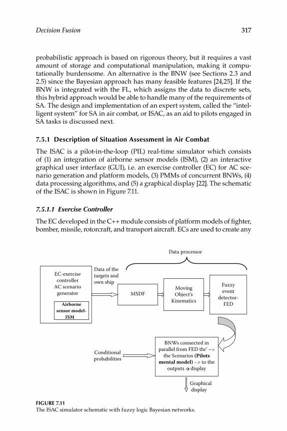
Decision Fusion 317

probabilistic approach is based on rigorous theory, but it requires a vast amount of storage and computational manipulation, making it compu-tationally burdensome. An alternative is the BNW (see Sections 2.3 and 2.5) since the Bayesian approach has many feasible features [24,25]. If the BNW is integrated with the FL, which assigns the data to discrete sets, this hybrid approach would be able to handle many of the requirements of SA. The design and implementation of an expert system, called the “intel-ligent system” for SA in air combat, or ISAC, as an aid to pilots engaged in SA tasks is discussed next.

7.5.1 Description of Situation Assessment in Air Combat

The ISAC is a pilot-in-the-loop (PIL) real-time simulator which consists of (1) an integration of airborne sensor models (ISM), (2) an interactive graphical user interface (GUI), i.e. an exercise controller (EC) for AC sce-nario generation and platform models, (3) PMMs of concurrent BNWs, (4) data processing algorithms, and (5) a graphical display [22]. The schematic of the ISAC is shown in Figure 7.11.

7.5.1.1 Exercise Controller

The EC developed in the C++ module consists of platform models of fi ghter, bomber, missile, rotorcraft, and transport aircraft. ECs are used to create any

FIGURE 7.11 The ISAC simulator schematic with fuzzy logic Bayesian networks.

EC-exercisecontroller

AC scenariogenerator

Airbornesensor model-

ISM

MSDFMovingObject’s

Kinematics

Fuzzyevent

detector-FED

BNWs connected inparallel from FED thr’ –>

the Scenarios (Pilotsmental model) –> to the

outputs display

Conditionalprobabilities

Graphicaldisplay

Data of thetargets andown ship

Data processor

318 Multi-Sensor Data Fusion: Theory and Practice

typical air-to-air combat scenarios, which can have a maximum of six targets (excluding the owner’s ship). ECs have a simple user interface consisting of a display area, status area, and menu area. The status area has important parameters such as speed, course, bearing, coordinates, and radar status. The targets are represented by prespecifi ed shapes and colors, which dis-tinguish the platform types they represent. The class and identifi cation of all targets should be specifi ed for the simulation. Each target is controlled either by predefi ned trajectories or by user interaction in real time.

7.5.1.2 Integrated Sensor Model

The integrated sensor model is a MATLAB-SIMULINK–based module that has functional models of different sensors: (1) Doppler radar, (2) IRST, (3) RWR, and (4) electro-optical tracking system.

7.5.1.3 Data Processor

The data processor (DP) module consists of (1) MSDF, (2) relative kine-matics data (RKD), and (3) fuzzy event detector (FED), and combines and classifi es data received from multiple sensors. EKF is used to estimate the states of the targets using fused measurements from multiple sensors. FED classifi es the RKD data into qualitative forms or events: the speed is “low,” “medium,” or “high.” The MATLAB FL toolbox is used to design appropriate membership functions for data classifi cation.

7.5.1.4 Pilot Mental Model

The PMM emulates the pilot’s information processing, SA, and decision-making functions based on information received from the DP. Agents based on BNW technology are used to assess the occurrence of different situations in AC scenarios using the HUGIN C++ API software tool [26].

Finally, the graphical display provides the updated probabilities of all the agents.

7.5.2 Bayesian Mental Model

A mental model of the SA requires (1) the capability to quantitatively represent key SA concepts such as situations, events, and the PMM; (2) a mechanism to refl ect both diagnostic and inferential reasoning; and (3) the ability to deal with various levels and types of uncertainties [21–25]. BNWs are ideal tools for meeting such requirements. BNWs are directed acyclic graphs in which the nodes represent probabilistic vari-ables whose probability distribution is denoted as a belief value (more so for the D–S belief NWs), and in which links represent informal or causal

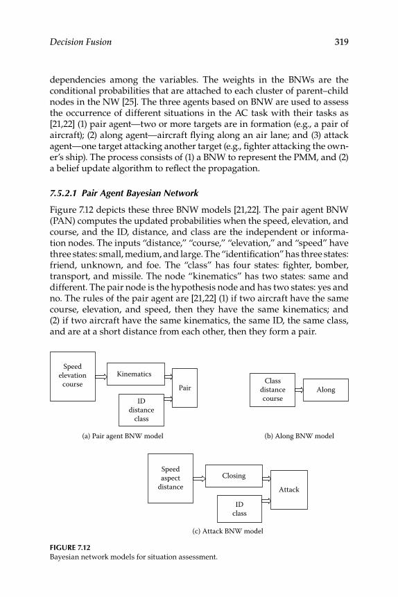
Decision Fusion 319

dependencies among the variables. The weights in the BNWs are the conditional probabilities that are attached to each cluster of parent–child nodes in the NW [25]. The three agents based on BNW are used to assess the occurrence of different situations in the AC task with their tasks as [21,22] (1) pair agent—two or more targets are in formation (e.g., a pair of aircraft); (2) along agent—aircraft fl ying along an air lane; and (3) attack agent—one target attacking another target (e.g., fi ghter attacking the own-er’s ship). The process consists of (1) a BNW to represent the PMM, and (2) a belief update algorithm to refl ect the propagation.

7.5.2.1 Pair Agent Bayesian Network

Figure 7.12 depicts these three BNW models [21,22]. The pair agent BNW (PAN) computes the updated probabilities when the speed, elevation, and course, and the ID, distance, and class are the independent or informa-tion nodes. The inputs “distance,” “course,” “elevation,” and “speed” have three states: small, medium, and large. The “identifi cation” has three states: friend, unknown, and foe. The “class” has four states: fi ghter, bomber, transport, and missile. The node “kinematics” has two states: same and different. The pair node is the hypothesis node and has two states: yes and no. The rules of the pair agent are [21,22] (1) if two aircraft have the same course, elevation, and speed, then they have the same kinematics; and (2) if two aircraft have the same kinematics, the same ID, the same class, and are at a short distance from each other, then they form a pair.

FIGURE 7.12 Bayesian network models for situation assessment.

Speedelevation

courseKinematics

PairID

distanceclass

Classdistancecourse

Along

(a) Pair agent BNW model (b) Along BNW model

ClosingSpeedaspect

distance Attack

IDclass

(c) Attack BNW model

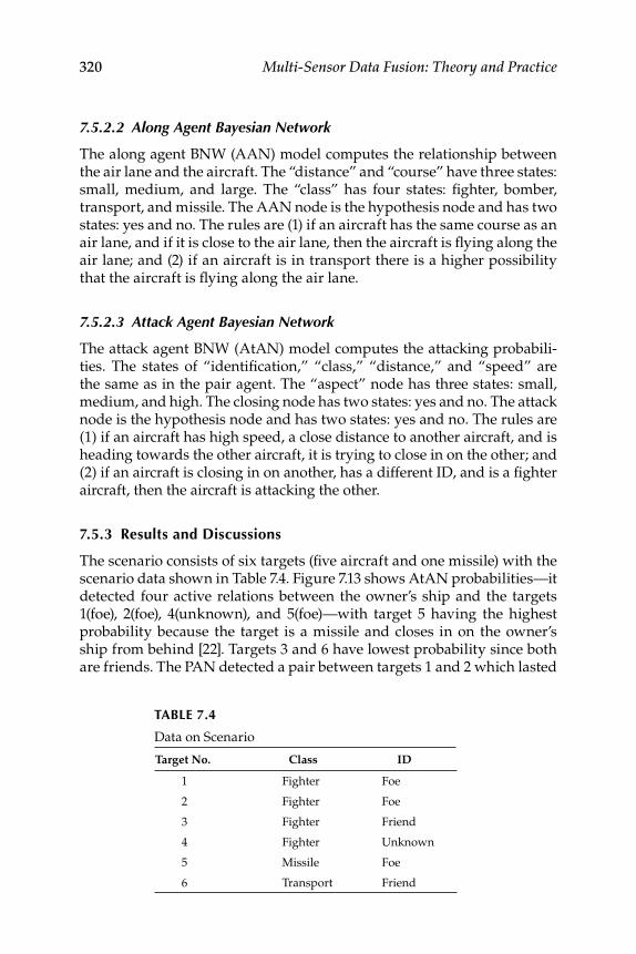
320 Multi-Sensor Data Fusion: Theory and Practice

7.5.2.2 Along Agent Bayesian Network

The along agent BNW (AAN) model computes the relationship between the air lane and the aircraft. The “distance” and “course” have three states: small, medium, and large. The “class” has four states: fi ghter, bomber, transport, and missile. The AAN node is the hypothesis node and has two states: yes and no. The rules are (1) if an aircraft has the same course as an air lane, and if it is close to the air lane, then the aircraft is fl ying along the air lane; and (2) if an aircraft is in transport there is a higher possibility that the aircraft is fl ying along the air lane.

7.5.2.3 Attack Agent Bayesian Network

The attack agent BNW (AtAN) model computes the attacking probabili-ties. The states of “identifi cation,” “class,” “distance,” and “speed” are the same as in the pair agent. The “aspect” node has three states: small, medium, and high. The closing node has two states: yes and no. The attack node is the hypothesis node and has two states: yes and no. The rules are (1) if an aircraft has high speed, a close distance to another aircraft, and is heading towards the other aircraft, it is trying to close in on the other; and (2) if an aircraft is closing in on another, has a different ID, and is a fi ghter aircraft, then the aircraft is attacking the other.

7.5.3 Results and Discussions

The scenario consists of six targets (fi ve aircraft and one missile) with the scenario data shown in Table 7.4. Figure 7.13 shows AtAN probabilities—it detected four active relations between the owner’s ship and the targets 1(foe), 2(foe), 4(unknown), and 5(foe)—with target 5 having the highest probability because the target is a missile and closes in on the owner’s ship from behind [22]. Targets 3 and 6 have lowest probability since both are friends. The PAN detected a pair between targets 1 and 2 which lasted

TABLE 7.4

Data on Scenario

Target No. Class ID

1 Fighter Foe

2 Fighter Foe

3 Fighter Friend

4 Fighter Unknown

5 Missile Foe

6 Transport Friend

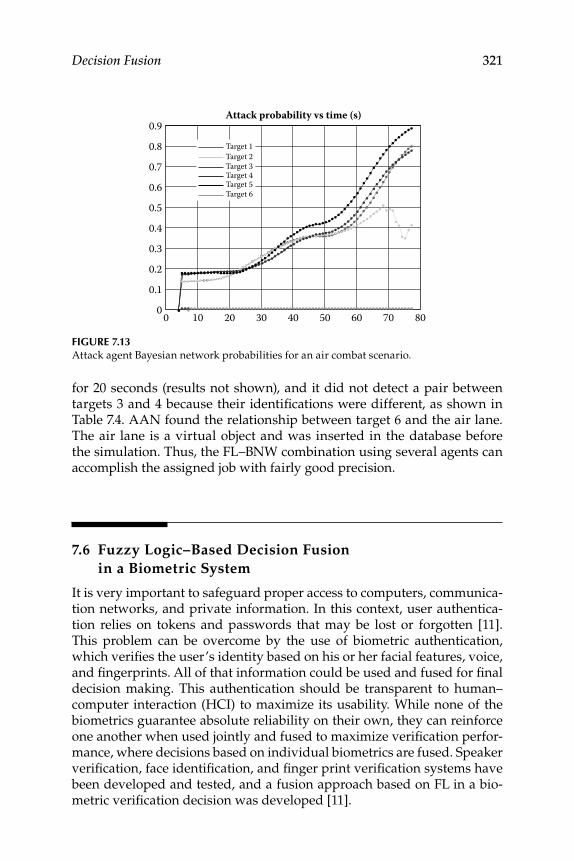
Decision Fusion 321

for 20 seconds (results not shown), and it did not detect a pair between targets 3 and 4 because their identifi cations were different, as shown in Table 7.4. AAN found the relationship between target 6 and the air lane. The air lane is a virtual object and was inserted in the database before the simulation. Thus, the FL–BNW combination using several agents can accomplish the assigned job with fairly good precision.

7.6 Fuzzy Logic–Based Decision Fusion

in a Biometric System

It is very important to safeguard proper access to computers, communica-tion networks, and private information. In this context, user authentica-tion relies on tokens and passwords that may be lost or forgotten [11]. This problem can be overcome by the use of biometric authentication, which verifi es the user’s identity based on his or her facial features, voice, and fi ngerprints. All of that information could be used and fused for fi nal decision making. This authentication should be transparent to human–computer interaction (HCI) to maximize its usability. While none of the biometrics guarantee absolute reliability on their own, they can reinforce one another when used jointly and fused to maximize verifi cation perfor-mance, where decisions based on individual biometrics are fused. Speaker verifi cation, face identifi cation, and fi nger print verifi cation systems have been developed and tested, and a fusion approach based on FL in a bio-metric verifi cation decision was developed [11].

FIGURE 7.13 Attack agent Bayesian network probabilities for an air combat scenario.

0.9Attack probability vs time (s)

0.8

0.7

0.6

0.5

0.4

0.3

0.2

0.1

0 0 10 20 30 40 50 60 70 80

Target 1Target 2Target 3Target 4Target 5Target 6

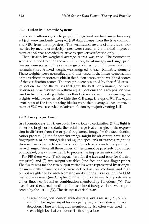
322 Multi-Sensor Data Fusion: Theory and Practice

7.6.1 Fusion in Biometric Systems

One speech utterance, one fi ngerprint image, and one face image for every subject were randomly grouped (480 data groups from the true claimant and 7200 from the imposters). The verifi cation results of individual bio-metrics by means of majority votes were fused, and a marked improve-ment of 48% was recorded, relative to speaker verifi cation only.

Then, fusion by weighted average scores was tried. The verifi cation scores obtained from the spoken utterances, facial images, and fi ngerprint images were scaled to the same range of values by minimum–maximum normalization. A fi xed weight was assigned to each biometric element. These weights were normalized and then used in the linear combination of the verifi cation scores to obtain the fusion score, or the weighted scores of the verifi cation scores. The weights were assigned by threefold cross-validation. To fi nd the values that gave the best performance, the veri-fi cation set was divided into three equal portions and each portion was used in turn for testing while the other two were used for optimizing the weights, which were varied within the [0, 1] range in steps of 0.1. The equal error rates of the three testing blocks were then averaged. An improve-ment of 52% was recorded, relative to fusion by majority voting [11].

7.6.2 Fuzzy Logic Fusion

In a biometric system, there could be various uncertainties: (1) the light is either too bright or too dark, the facial image is at an angle, or the expres-sion is different from the original registered image for the face identifi -cation process; (2) the fi ngerprint image might be off-center, have faded fi ngerprints, or be smudged; and (3) the speaker’s utterances might be drowned in noise or his or her voice characteristics and/or style might have changed. Since all these uncertainties cannot be precisely quantifi ed or modeled, one can use the FL to process the imprecise information.

For FIS there were (1) six inputs (two for the face and four for the fi n-ger print), and (2) two output variables (one face and one fi nger print). The fuzzy sets for the two output variables were represented by triangu-lar membership functions and were defi ned as low, medium, and high output weightings for each biometric entity. For defuzzifi cation, the COA method was used (see Chapter 6). The input variables’ fuzzy sets were either linear or Gaussian combination membership functions, f ( x ). The least favored external condition for each input fuzzy variable was repre-sented by the set 1 − f ( x ). The six input variables are

1. “Face-fi nding confi dence” with discrete levels set as 0, 2.5, 5, 7.5, and 10. The higher input levels signify higher confi dence in face detection. Here a triangular membership function was used to seek a high level of confi dence in fi nding a face.

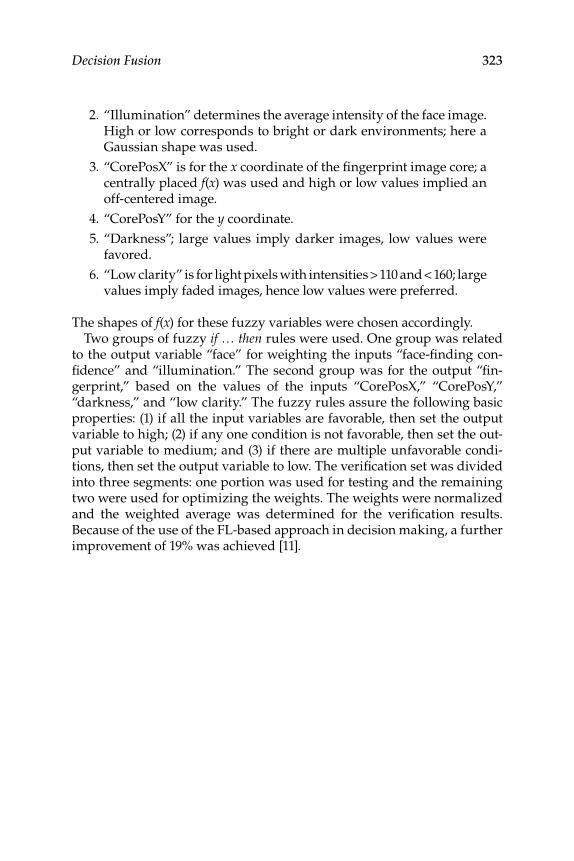
Decision Fusion 323

2. “Illumination” determines the average intensity of the face image. High or low corresponds to bright or dark environments; here a Gaussian shape was used.

3. “CorePosX” is for the x coordinate of the fi ngerprint image core; a centrally placed f ( x ) was used and high or low values implied an off-centered image.

4. “CorePosY” for the y coordinate.

5. “Darkness”; large values imply darker images, low values were favored.

6. “Low clarity” is for light pixels with intensities > 110 and < 160; large values imply faded images, hence low values were preferred.

The shapes of f ( x ) for these fuzzy variables were chosen accordingly. Two groups of fuzzy if … then rules were used. One group was related

to the output variable “face” for weighting the inputs “face-fi nding con-fi dence” and “illumination.” The second group was for the output “fi n-gerprint,” based on the values of the inputs “CorePosX,” “CorePosY,” “darkness,” and “low clarity.” The fuzzy rules assure the following basic properties: (1) if all the input variables are favorable, then set the output variable to high; (2) if any one condition is not favorable, then set the out-put variable to medium; and (3) if there are multiple unfavorable condi-tions, then set the output variable to low. The verifi cation set was divided into three segments: one portion was used for testing and the remaining two were used for optimizing the weights. The weights were normalized and the weighted average was determined for the verifi cation results. Because of the use of the FL-based approach in decision making, a further improvement of 19% was achieved [11].

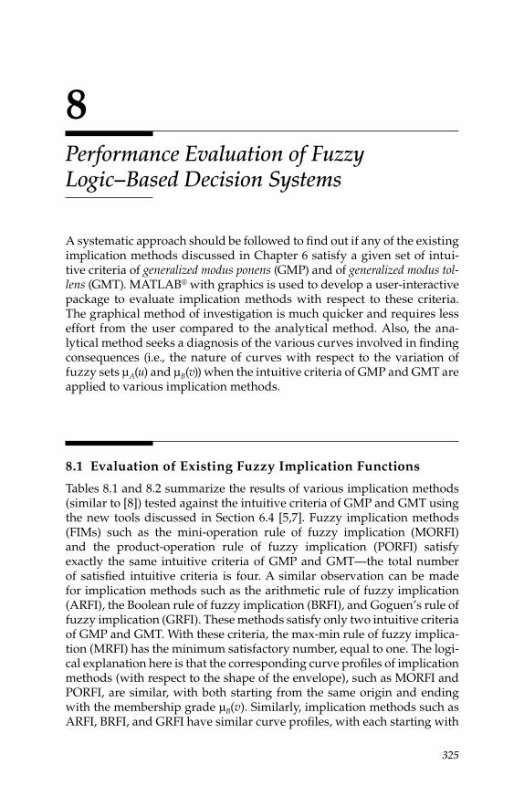
325

8 Performance Evaluation of Fuzzy Logic–Based Decision Systems

A systematic approach should be followed to fi nd out if any of the existing implication methods discussed in Chapter 6 satisfy a given set of intui-tive criteria of generalized modus ponens (GMP) and of generalized modus tol-lens (GMT). MATLAB® with graphics is used to develop a user-interactive package to evaluate implication methods with respect to these criteria. The graphical method of investigation is much quicker and requires less effort from the user compared to the analytical method. Also, the ana-lytical method seeks a diagnosis of the various curves involved in fi nding consequences (i.e., the nature of curves with respect to the variation of fuzzy sets μA(u) and μB(v)) when the intuitive criteria of GMP and GMT are applied to various implication methods.

8.1 Evaluation of Existing Fuzzy Implication Functions

Tables 8.1 and 8.2 summarize the results of various implication methods (similar to [8]) tested against the intuitive criteria of GMP and GMT using the new tools discussed in Section 6.4 [5,7]. Fuzzy implication methods (FIMs) such as the mini-operation rule of fuzzy implication (MORFI) and the product-operation rule of fuzzy implication (PORFI) satisfy exactly the same intuitive criteria of GMP and GMT—the total number of satisfi ed intuitive criteria is four. A similar observation can be made for implication methods such as the arithmetic rule of fuzzy implication (ARFI), the Boolean rule of fuzzy implication (BRFI), and Goguen’s rule of fuzzy implication (GRFI). These methods satisfy only two intuitive criteria of GMP and GMT. With these criteria, the max-min rule of fuzzy implica-tion (MRFI) has the minimum satisfactory number, equal to one. The logi-cal explanation here is that the corresponding curve profi les of implication methods (with respect to the shape of the envelope), such as MORFI and PORFI, are similar, with both starting from the same origin and ending with the membership grade μB(v). Similarly, implication methods such as ARFI, BRFI, and GRFI have similar curve profi les, with each starting with

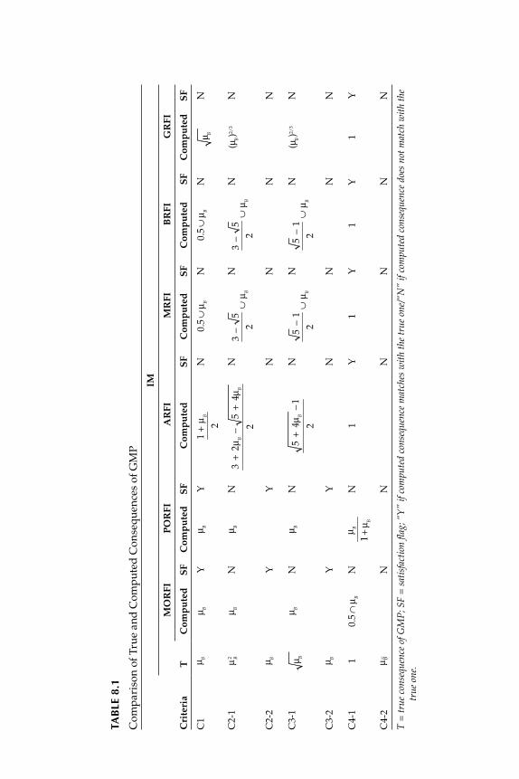
TAB

LE 8

.1

Co

mp

ari

son

of

Tru

e a

nd

Co

mp

ute

d C

on

seq

uen

ces

of

GM

P

Cri

teri

a

IM

T

MO

RF

IP

OR

FI

AR

FI

MR

FI

BR

FI

GR

FI

Co

mp

ute

dS

FC

om

pu

ted

SF

Co

mp

ute

dS

FC

om

pu

ted

SF

Co

mp

ute

dS

FC

om

pu

ted

SF

C1

μ Bμ B

Yμ B

Y1

+μ B

2

N0.5

∪μ B

N0.5

∪μ B

Nμ B

N

C2-1

μ2 Bμ B

Nμ B

N3

+2

μ B−

5+

4μ B

2

N3

−5

2∪

μ B

N3

−5

2∪

μ B

N(μ

B)2/

3N

C2-2

μ BY

YN

NN

N

C3-1

μ B

μ BN

μ BN

5+

4μ B

−1

2

N5

−1

2∪

μ B

N5

−1

2∪

μ B

N(μ

B)2/

3N

C3-2

μ BY

YN

NN

N

C4-1

10.5

∩μ B

Nμ B

1+

μ B

N1

Y1

Y1

Y1

Y

C4-2

μ B_N

NN

NN

N

T =

tru

e co

nseq

uenc

e of

GM

P; S

F =

sat

isfa

ctio

n fl a

g; “

Y”

if co

mpu

ted

cons

eque

nce

mat

ches

wit

h th

e tr

ue o

ne/“

N”

if co

mpu

ted

cons

eque

nce

does

not

mat

ch w

ith

the

true

one

.

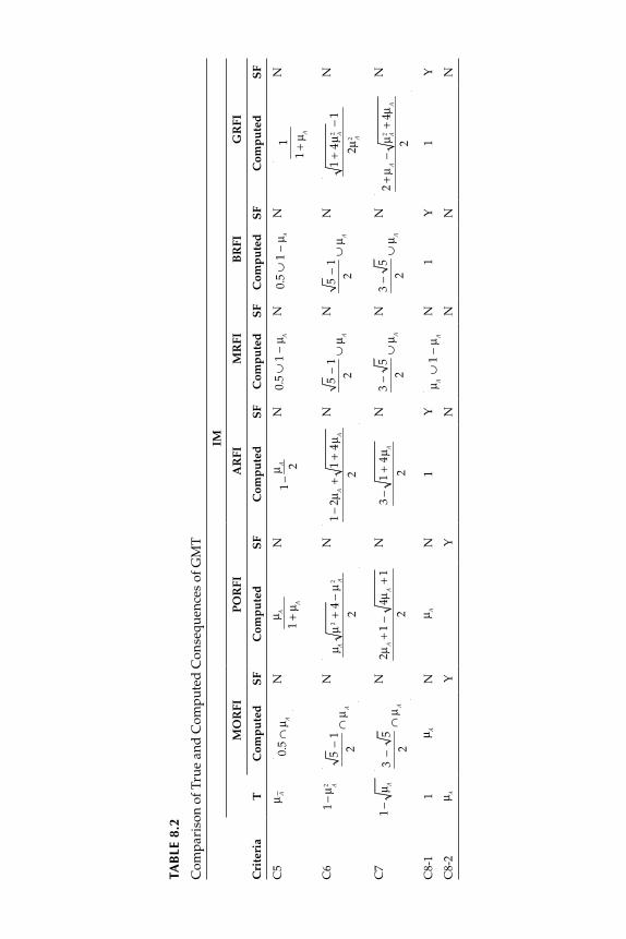
TAB

LE 8

.2

Co

mp

ari

son

of

Tru

e a

nd

Co

mp

ute

d C

on

seq

uen

ces

of

GM

T

Cri

teri

a

IM

T

MO

RF

IP

OR

FI

AR

FI

MR

FI

BR

FI

GR

FI

Co

mp

ute

dS

FC

om

pu

ted

SF

Co

mp

ute

dS

FC

om

pu

ted

SF

Co

mp

ute

dS

FC

om

pu

ted

SF

C5

μA

0.5

∩μ A

Nμ A

1+

μ A

N1

−μ

A 2

N0.5

∪1

−μ A

N0.5

∪1

−μ A

N

1

1+

μ A

N

C6

1−

μ2 A

5−

1

2∩

μA

N

μ Aμ

2+

4−

μ2 A

2

N

1−

2μ A

+1

+4

μ A

2

N5

−1

2∪

μ A

N5

−1

2∪

μ A

N

1+

4μ2 A

−1

2μ2 A

N

C7

1−

μ A

3−

5

2∩

μA

N2

μ A+

1−

4μ A

+1

2

N3

−1

+4

μ A

2

N3

−5

2∪

μ A

N3

−5

2∪

μ A

N

2+

μA

−μ2 A

+4μ

A

2

N

C8-1

1μ A

Nμ A

N1

Y μ A

∪1

−μ A

N1

Y1

Y

C8-2

μ AY

YN

NN

N

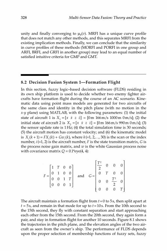
328 Multi-Sensor Data Fusion: Theory and Practice

unity and fi nally converging to μB(v). MRFI has a unique curve profi le that does not match any other methods, and this separates MRFI from the existing implication methods. Finally, we can conclude that the similarity in curve profi les of these methods (MORFI and PORFI in one group and ARFI, BRFI, and GRFI in another group) may lead to an equal number of satisfi ed intuitive criteria for GMP and GMT.

8.2 Decision Fusion System 1—Formation Flight

In this section, fuzzy logic–based decision software (FLDS) residing in its own ship platform is used to decide whether two enemy fi ghter air-crafts have formation fl ight during the course of an AC scenario. Kine-matic data using point mass models are generated for two aircrafts of the same class and identity in the pitch plane (with no motion in the x-y plane) using MATLAB, with the following parameters: (1) the initial

state of aircraft 1 is X1

= [x &x z &z] = [0 m 166 m/s 1000 m 0 m/s]; (2) the

initial state of aircraft 2 is X2= [x &x z &z] = [0 m 166 m/s 990 m 0 m/s]; (3)

the sensor update rate is 1 Hz; (4) the total simulation time is 30 seconds; (5) the aircraft motion has constant velocity; and (6) the kinematic model

is Xi (k + 1) = FXi (k) + Gwi (k), where k (=1, 2,…, 30) is the scan or the index

number, i (=1, 2) is the aircraft number, F is the state transition matrix, G is the process noise gain matrix, and w is the white Gaussian process noise with covariance matrix Q = 0.1*eye(4, 4):

F =

1 T 0 0

0 1 0 0

0 0 1 T

0 0 0 1

⎡

⎣

⎢⎢⎢⎢

⎤

⎦

⎥⎥⎥⎥

and

G =

T 2

20 0 0

0 T 0 0

0 0T 2

20

0 0 0 T

⎡

⎣

⎢⎢⎢⎢⎢⎢⎢

⎤

⎦

⎥⎥⎥⎥⎥⎥⎥

The aircraft maintain a formation fl ight from t = 0 to 5 s, then split apart at t = 5 s, and remain in that mode for up to t = 10 s. From the 10th second to the 15th second, they fl y with constant separation and start approaching each other from the 15th second. From the 20th second, they again form a pair, and stay in formation fl ight for another 10 seconds. Figure 8.1 shows the trajectories in the pitch plane, and the elevation angles of the two air-craft as seen from the owner’s ship. The performance of FLDS depends upon the proper selection of membership functions of fuzzy sets, fuzzy

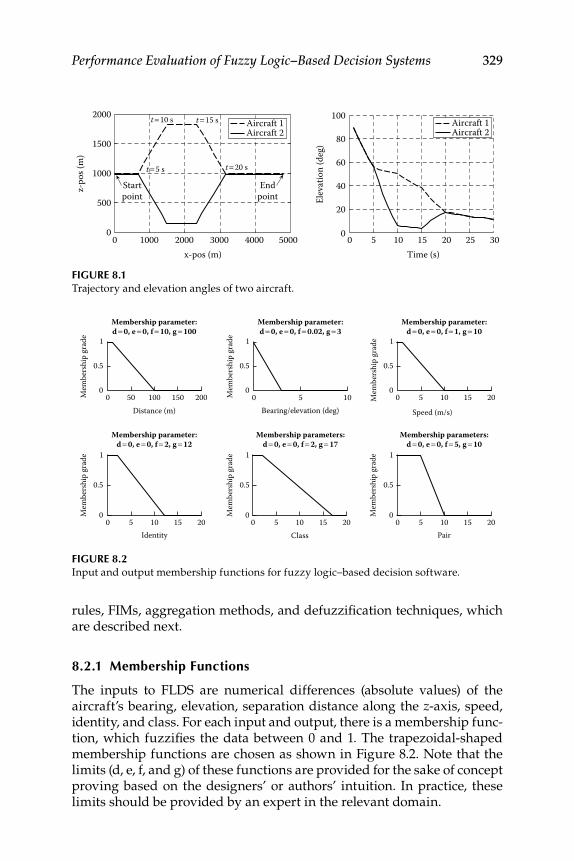
Performance Evaluation of Fuzzy Logic–Based Decision Systems 329

rules, FIMs, aggregation methods, and defuzzifi cation techniques, which are described next.

8.2.1 Membership Functions

The inputs to FLDS are numerical differences (absolute values) of the aircraft’s bearing, elevation, separation distance along the z -axis, speed, identity, and class. For each input and output, there is a membership func-tion, which fuzzifi es the data between 0 and 1. The trapezoidal-shaped membership functions are chosen as shown in Figure 8.2. Note that the limits (d, e, f, and g) of these functions are provided for the sake of concept proving based on the designers’ or authors’ intuition. In practice, these limits should be provided by an expert in the relevant domain.

FIGURE 8.1 Trajectory and elevation angles of two aircraft.

0 1000 2000 3000 4000 50000

500

1000

1500

2000

0 5 10 15 20 25 300

20

40

60

80

100

z-po

s (m

)

Time (s)x-pos (m)

t = 15 st = 10 s

t = 5 s t = 20 s

Endpoint

Startpoint El

evat

ion

(deg

)

Aircraft 2Aircraft 1

Aircraft 2Aircraft 1

FIGURE 8.2 Input and output membership functions for fuzzy logic–based decision software.

Bearing/elevation (deg)

0.5

Mem

bers

hip

grad

e

00 50 100

Distance (m)150 200

1

Membership parameter:d = 0, e = 0, f = 10, g = 100

Membership parameter:d = 0, e = 0, f = 0.02, g = 3

Membership parameter:d = 0, e = 0, f = 1, g = 10

Membership parameter:d = 0, e = 0, f = 2, g = 12

Membership parameters:d = 0, e = 0, f = 2, g = 17

Membership parameters:d = 0, e = 0, f = 5, g = 10

0.5

Mem

bers

hip

grad

e

00 5 10

Identity15 20

1

0.5

Mem

bers

hip

grad

e

00 5 10

Class15 20

1

0.5

Mem

bers

hip

grad

e

00 5 10

Pair15 20

1

0.5M

embe

rshi

p gr

ade

00 5 10

Speed (m/s)

15 20

1

0.5

Mem

bers

hip

grad

e

00 5 10

1

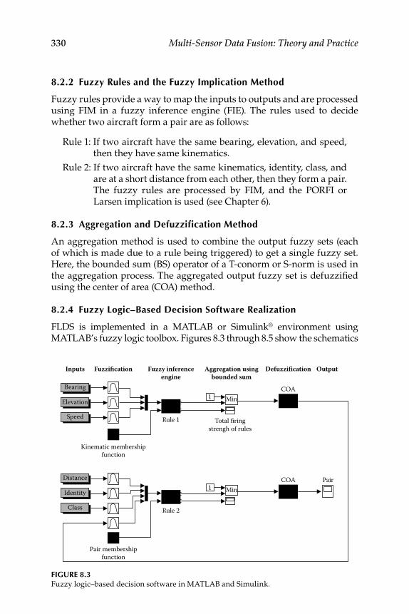
330 Multi-Sensor Data Fusion: Theory and Practice

8.2.2 Fuzzy Rules and the Fuzzy Implication Method

Fuzzy rules provide a way to map the inputs to outputs and are processed using FIM in a fuzzy inference engine (FIE). The rules used to decide whether two aircraft form a pair are as follows:

Rule 1: If two aircraft have the same bearing, elevation, and speed, then they have same kinematics.

Rule 2: If two aircraft have the same kinematics, identity, class, and are at a short distance from each other, then they form a pair. The fuzzy rules are processed by FIM, and the PORFI or Larsen implication is used (see Chapter 6).

8.2.3 Aggregation and Defuzzification Method

An aggregation method is used to combine the output fuzzy sets (each of which is made due to a rule being triggered) to get a single fuzzy set. Here, the bounded sum (BS) operator of a T-conorm or S-norm is used in the aggregation process. The aggregated output fuzzy set is defuzzifi ed using the center of area (COA) method.

8.2.4 Fuzzy Logic–Based Decision Software Realization

FLDS is implemented in a MATLAB or Simulink® environment using MATLAB’s fuzzy logic toolbox. Figures 8.3 through 8.5 show the schematics

FIGURE 8.3 Fuzzy logic–based decision software in MATLAB and Simulink.

Bearing

Inputs Fuzzification Fuzzy inferenceengine

Aggregation usingbounded sum

Defuzzif ication Output

Speed Rule 1 Total firingstrengh of rules

Kinematic membershipfunction

COAMin1

Elevation

Distance

Class Rule 2

Pair membershipfunction

COA PairMin1

Identity

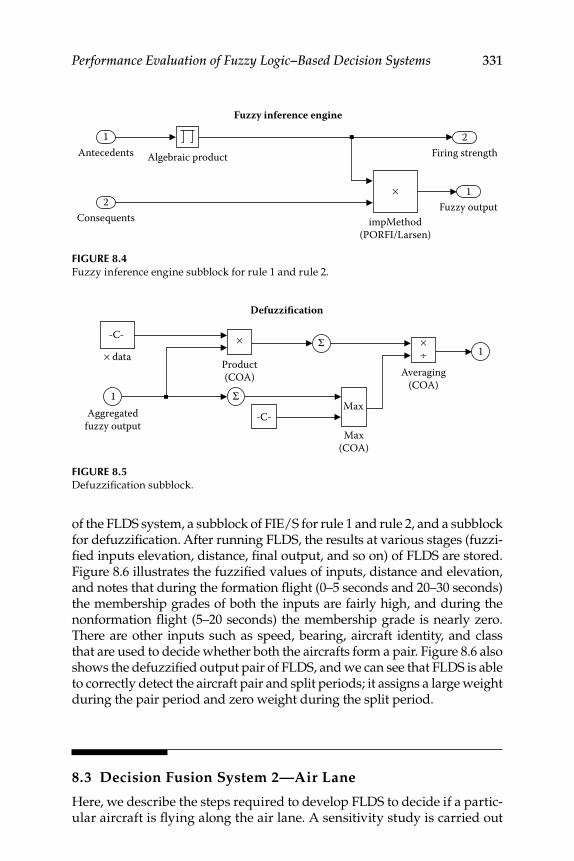
Performance Evaluation of Fuzzy Logic–Based Decision Systems 331

of the FLDS system, a subblock of FIE/S for rule 1 and rule 2, and a subblock for defuzzifi cation. After running FLDS, the results at various stages (fuzzi-fi ed inputs elevation, distance, fi nal output, and so on) of FLDS are stored. Figure 8.6 illustrates the fuzzifi ed values of inputs, distance and elevation, and notes that during the formation fl ight (0–5 seconds and 20–30 seconds) the membership grades of both the inputs are fairly high, and during the nonformation fl ight (5–20 seconds) the membership grade is nearly zero. There are other inputs such as speed, bearing, aircraft identity, and class that are used to decide whether both the aircrafts form a pair. Figure 8.6 also shows the defuzzifi ed output pair of FLDS, and we can see that FLDS is able to correctly detect the aircraft pair and split periods; it assigns a large weight during the pair period and zero weight during the split period.

8.3 Decision Fusion System 2—Air Lane

Here, we describe the steps required to develop FLDS to decide if a partic-ular aircraft is fl ying along the air lane. A sensitivity study is carried out

FIGURE 8.5Defuzzifi cation subblock.

Defuzzification

1

-C-

-C-Aggregatedfuzzy output

Max(COA)

Averaging(COA)

Product(COA)

× data 1

Σ

Σ× ×÷

Max

FIGURE 8.4Fuzzy inference engine subblock for rule 1 and rule 2.

Fuzzy inference engine

1

Algebraic productAntecedents

Consequents impMethod(PORFI/Larsen)

Fuzzy output

Firing strength

21

2

×

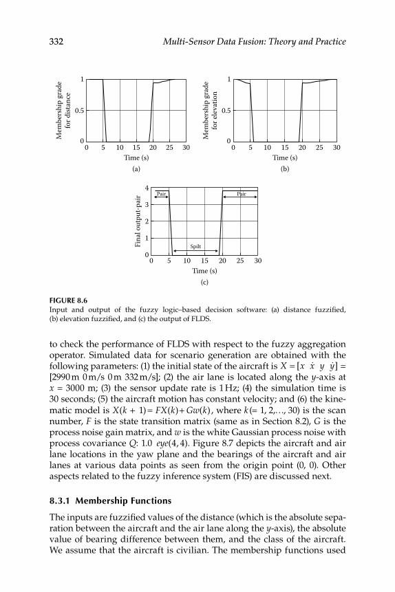
332 Multi-Sensor Data Fusion: Theory and Practice

to check the performance of FLDS with respect to the fuzzy aggregation operator. Simulated data for scenario generation are obtained with the following parameters: (1) the initial state of the aircraft is X = [x &x y &y] = [2990 m 0 m/s 0 m 332 m/s]; (2) the air lane is located along the y -axis at x = 3000 m; (3) the sensor update rate is 1 Hz; (4) the simulation time is 30 seconds; (5) the aircraft motion has constant velocity; and (6) the kine-

matic model is X(k + 1) = FX(k)+ Gw(k), where k (= 1, 2,…, 30) is the scan number, F is the state transition matrix (same as in Section 8.2), G is the process noise gain matrix, and w is the white Gaussian process noise with process covariance Q : 1.0

eye(4, 4). Figure 8.7 depicts the aircraft and air lane locations in the yaw plane and the bearings of the aircraft and air lanes at various data points as seen from the origin point (0, 0). Other aspects related to the fuzzy inference system (FIS) are discussed next.

8.3.1 Membership Functions

The inputs are fuzzifi ed values of the distance (which is the absolute sepa-ration between the aircraft and the air lane along the y -axis), the absolute value of bearing difference between them, and the class of the aircraft. We assume that the aircraft is civilian. The membership functions used

FIGURE 8.6Input and output of the fuzzy logic–based decision software: (a) distance fuzzifi ed,

(b) elevation fuzzifi ed, and (c) the output of FLDS.

1

0.5

00M

embe

rshi

p gr

ade

for d

istan

ce

5 10 15Time (s)

20 25 30

(a)

1

0.5

00M

embe

rshi

p gr

ade

for e

levat

ion

5 10 15Time (s)

20 25 30

(b)

0

Fina

l out

put-p

air

0

1

2

3

4

Spilt

5 10 15Time (s)

20 25 30

PairPair

(c)

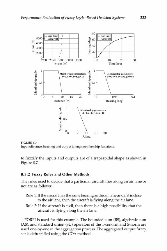
Performance Evaluation of Fuzzy Logic–Based Decision Systems 333

to fuzzify the inputs and outputs are of a trapezoidal shape as shown in Figure 8.7.

8.3.2 Fuzzy Rules and Other Methods

The rules used to decide that a particular aircraft fl ies along an air lane or not are as follows:

Rule 1: If the aircraft has the same bearing as the air lane and if it is close to the air lane, then the aircraft is fl ying along the air lane.

Rule 2: If the aircraft is civil, then there is a high possibility that the aircraft is fl ying along the air lane.

PORFI is used for this example. The bounded sum (BS), algebraic sum (AS), and standard union (SU) operators of the T-conorm and S-norm are used one-by-one in the aggregation process. The aggregated output fuzzy set is defuzzifi ed using the COA method.

FIGURE 8.7 Input (distance, bearing) and output (along) membership functions.

3100x-pos (m)

3050300029502900

8000

1

0.5

0 0 5 10Distance (m)

Mem

bers

hip

grad

e

15 20

80

60

40

Bear

ing (

deg)

y-po

s(m

)

20

0 0 10 20 30Time (sec)

600040002000

0

Air laneAircraft

Air laneAircraft

Membership parameters:d = 0, e = 0 , f = 8, g = 10

1

0.5

00 5 10

Mem

bers

hip

grad

e

15 20

Membership parameters:d = 0, e = 0, f = 5, g = 10

1

0.5

00 0.05Bearing (deg)

Along

Mem

bers

hip

grad

e

0.1

Membership parameters:d = 0, e = 0, f = 0.02, g = 0.04

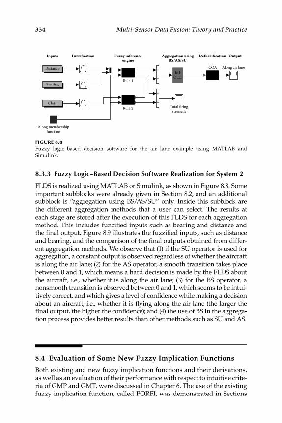
334 Multi-Sensor Data Fusion: Theory and Practice

8.3.3 Fuzzy Logic–Based Decision Software Realization for System 2

FLDS is realized using MATLAB or Simulink, as shown in Figure 8.8. Some important subblocks were already given in Section 8.2, and an additional subblock is “aggregation using BS/AS/SU” only. Inside this subblock are the different aggregation methods that a user can select. The results at each stage are stored after the execution of this FLDS for each aggregation method. This includes fuzzifi ed inputs such as bearing and distance and the fi nal output. Figure 8.9 illustrates the fuzzifi ed inputs, such as distance and bearing, and the comparison of the fi nal outputs obtained from differ-ent aggregation methods. We observe that (1) if the SU operator is used for aggregation, a constant output is observed regardless of whether the aircraft is along the air lane; (2) for the AS operator, a smooth transition takes place between 0 and 1, which means a hard decision is made by the FLDS about the aircraft, i.e., whether it is along the air lane; (3) for the BS operator, a nonsmooth transition is observed between 0 and 1, which seems to be intui-tively correct, and which gives a level of confi dence while making a decision about an aircraft, i.e., whether it is fl ying along the air lane (the larger the fi nal output, the higher the confi dence); and (4) the use of BS in the aggrega-tion process provides better results than other methods such as SU and AS.

8.4 Evaluation of Some New Fuzzy Implication Functions

Both existing and new fuzzy implication functions and their derivations, as well as an evaluation of their performance with respect to intuitive crite-ria of GMP and GMT, were discussed in Chapter 6. The use of the existing fuzzy implication function, called PORFI, was demonstrated in Sections

FIGURE 8.8 Fuzzy logic–based decision software for the air lane example using MATLAB and

Simulink.

Bearing

Distance

Class

Inputs Fuzzification Fuzzy inferenceengine

Aggregation usingBS/AS/SU

Defuzzif ication Output

Rule 1

Rule 2 Total firingstrength

COAIn1

Out1

Along air lane

Along membershipfunction

+

+

+

+

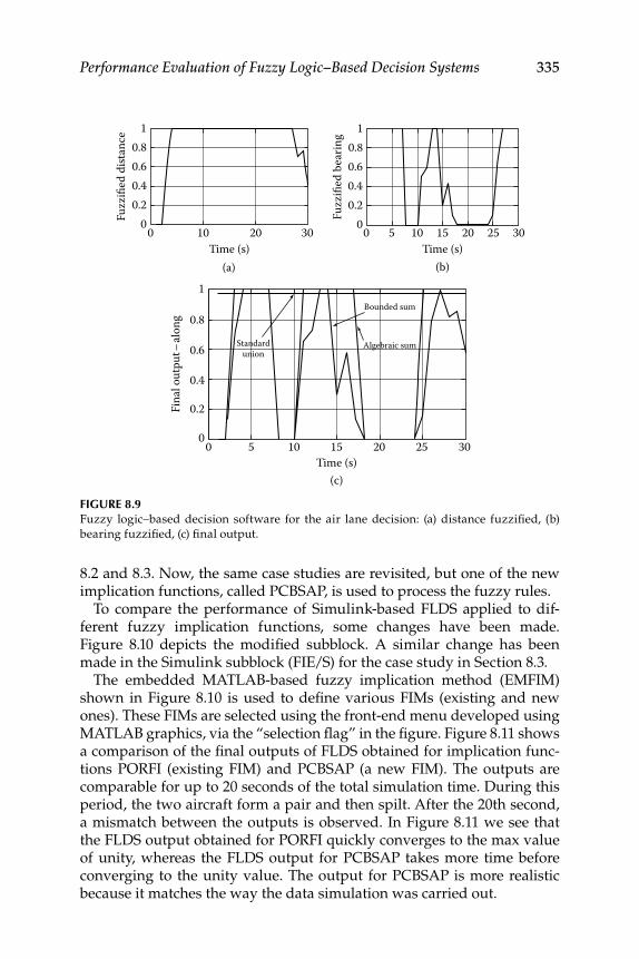
Performance Evaluation of Fuzzy Logic–Based Decision Systems 335

8.2 and 8.3. Now, the same case studies are revisited, but one of the new implication functions, called PCBSAP, is used to process the fuzzy rules.

To compare the performance of Simulink-based FLDS applied to dif-ferent fuzzy implication functions, some changes have been made. Figure 8.10 depicts the modifi ed subblock. A similar change has been made in the Simulink subblock (FIE/S) for the case study in Section 8.3.

The embedded MATLAB-based fuzzy implication method (EMFIM) shown in Figure 8.10 is used to defi ne various FIMs (existing and new ones). These FIMs are selected using the front-end menu developed using MATLAB graphics, via the “selection fl ag” in the fi gure. Figure 8.11 shows a comparison of the fi nal outputs of FLDS obtained for implication func-tions PORFI (existing FIM) and PCBSAP (a new FIM). The outputs are comparable for up to 20 seconds of the total simulation time. During this period, the two aircraft form a pair and then spilt. After the 20th second, a mismatch between the outputs is observed. In Figure 8.11 we see that the FLDS output obtained for PORFI quickly converges to the max value of unity, whereas the FLDS output for PCBSAP takes more time before converging to the unity value. The output for PCBSAP is more realistic because it matches the way the data simulation was carried out.

FIGURE 8.9 Fuzzy logic–based decision software for the air lane decision: (a) distance fuzzifi ed, (b)

bearing fuzzifi ed, (c) fi nal output.

Time (s) Time (s)(a) (b)

0 10 20 30 0 10 15 255 20 300

0.20.4

Fuzz

ified

dist

ance

Fuzz

ified

bea

ring

0.60.8

1

00.20.40.60.8

1

Time (s)

Fina

l out

put–

along

0

0.2

0.4

0 5 10 15 20 25 30

0.6 Standardunion

Algebraic sum

Bounded sum

1

0.8

(c)

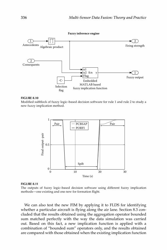
336 Multi-Sensor Data Fusion: Theory and Practice

We can also test the new FIM by applying it to FLDS for identifying whether a particular aircraft is fl ying along the air lane. Section 8.3 con-cluded that the results obtained using the aggregation operator bounded sum matched perfectly with the way the data simulation was carried out. Based on this fact, a new implication function is applied with a combination of “bounded sum” operators only, and the results obtained are compared with those obtained when the existing implication function

FIGURE 8.10 Modifi ed subblock of fuzzy logic–based decision software for rule 1 and rule 2 to study a

new fuzzy implication method.

1

Algebraic productAntecedents Firing strength2

Fuzzy outputEmbedded

MATLAB basedfuzzy implication functionSelection

flag

u1u2 fcn yFlag

21

Consequents2

-C-

Fuzzy inference engine

FIGURE 8.11 The outputs of fuzzy logic–based decision software using different fuzzy implication

methods—one existing and one new for formation fl ight.

00

0.5

Fina

l out

put-

pair

1

10Time (s)

20 30

Pair

Spilt

Pair PCBSAPPORFI

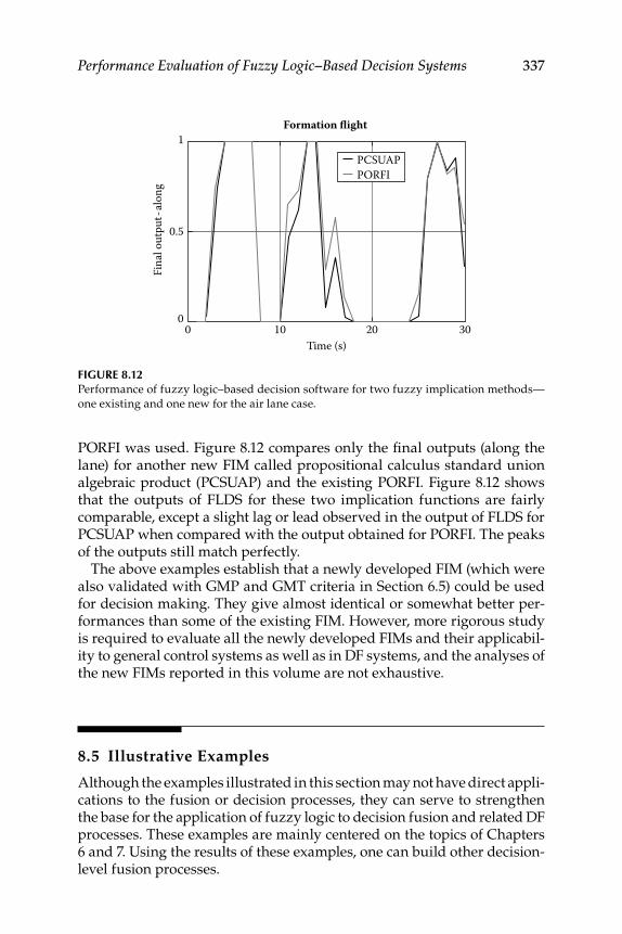
Performance Evaluation of Fuzzy Logic–Based Decision Systems 337

PORFI was used. Figure 8.12 compares only the fi nal outputs (along the lane) for another new FIM called propositional calculus standard union algebraic product (PCSUAP) and the existing PORFI. Figure 8.12 shows that the outputs of FLDS for these two implication functions are fairly comparable, except a slight lag or lead observed in the output of FLDS for PCSUAP when compared with the output obtained for PORFI. The peaks of the outputs still match perfectly.

The above examples establish that a newly developed FIM (which were also validated with GMP and GMT criteria in Section 6.5) could be used for decision making. They give almost identical or somewhat better per-formances than some of the existing FIM. However, more rigorous study is required to evaluate all the newly developed FIMs and their applicabil-ity to general control systems as well as in DF systems, and the analyses of the new FIMs reported in this volume are not exhaustive.

8.5 Illustrative Examples

Although the examples illustrated in this section may not have direct appli-cations to the fusion or decision processes, they can serve to strengthen the base for the application of fuzzy logic to decision fusion and related DF processes. These examples are mainly centered on the topics of Chapters 6 and 7. Using the results of these examples, one can build other decision-level fusion processes.

FIGURE 8.12 Performance of fuzzy logic–based decision software for two fuzzy implication methods—

one existing and one new for the air lane case.

00

0.5

Fina

l out

put-

along

1

10Time (s)

20 30

PCSUAPPORFI

Formation flight

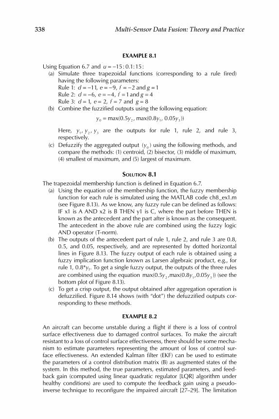
338 Multi-Sensor Data Fusion: Theory and Practice

EXAMPLE 8.1

Using Equation 6.7 and u = −15: 0.1:15: (a) Simulate three trapezoidal functions (corresponding to a rule fi red)

having the following parameters: Rule 1: d = −11, e = −9, f = −2 and g = 1 Rule 2: d = −6, e = −4, f = 1 and g = 4 Rule 3: d = 1, e = 2, f = 7 and g = 8 (b) Combine the fuzzifi ed outputs using the following equation:

y0 = max(0.5y2 , max(0.8y1, 0.05y3 ))

Here, y1, y2 , y3 are the outputs for rule 1, rule 2, and rule 3, respectively.

(c) Defuzzify the aggregated output (y0 ) using the following methods, and compare the methods: (1) centroid, (2) bisector, (3) middle of maximum, (4) smallest of maximum, and (5) largest of maximum.

SOLUTION 8.1 The trapezoidal membership function is defi ned in Equation 6.7.

(a) Using the equation of the membership function, the fuzzy membership function for each rule is simulated using the MATLAB code ch8_ex1.m (see Figure 8.13). As we know, any fuzzy rule can be defi ned as follows: IF x1 is A AND x2 is B THEN y1 is C, where the part before THEN is known as the antecedent and the part after is known as the consequent. The antecedent in the above rule are combined using the fuzzy logic AND operator (T-norm).

(b) The outputs of the antecedent part of rule 1, rule 2, and rule 3 are 0.8, 0.5, and 0.05, respectively, and are represented by dotted horizontal lines in Figure 8.13. The fuzzy output of each rule is obtained using a fuzzy implication function known as Larsen algebraic product, e.g., for rule 1, 0.8*y 1 . To get a single fuzzy output, the outputs of the three rules are combined using the equation max(0.5y2 ,max(0.8y1,0.05y3 )) (see the bottom plot of Figure 8.13).

(c) To get a crisp output, the output obtained after aggregation operation is defuzzifi ed. Figure 8.14 shows (with “dot”) the defuzzifi ed outputs cor-responding to these methods.

EXAMPLE 8.2

An aircraft can become unstable during a fl ight if there is a loss of control surface effectiveness due to damaged control surfaces. To make the aircraft resistant to a loss of control surface effectiveness, there should be some mecha-nism to estimate parameters representing the amount of loss of control sur-face effectiveness. An extended Kalman fi lter (EKF) can be used to estimate the parameters of a control distribution matrix (B) as augmented states of the system. In this method, the true parameters, estimated parameters, and feed-back gain (computed using linear quadratic regulator [LQR] algorithm under healthy conditions) are used to compute the feedback gain using a pseudo-inverse technique to reconfi gure the impaired aircraft [27–29]. The limitation

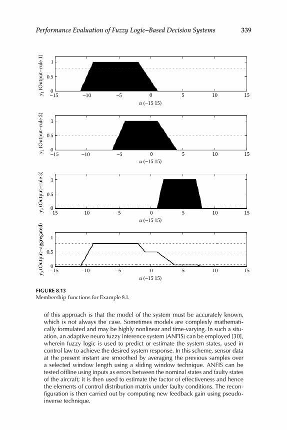
Performance Evaluation of Fuzzy Logic–Based Decision Systems 339

of this approach is that the model of the system must be accurately known, which is not always the case. Sometimes models are complexly mathemati-cally formulated and may be highly nonlinear and time-varying. In such a situ-ation, an adaptive neuro fuzzy inference system (ANFIS) can be employed [30], wherein fuzzy logic is used to predict or estimate the system states, used in control law to achieve the desired system response. In this scheme, sensor data at the present instant are smoothed by averaging the previous samples over a selected window length using a sliding window technique. ANFIS can be tested offl ine using inputs as errors between the nominal states and faulty states of the aircraft; it is then used to estimate the factor of effectiveness and hence the elements of control distribution matrix under faulty conditions. The recon-fi guration is then carried out by computing new feedback gain using pseudo-inverse technique.

FIGURE 8.13 Membership functions for Example 8.1.

−15 −10 −5 0 5 10 150

0.5

1

u (−15 15)

y 1 (O

utpu

t–ru

le 1)

−15 −10 −5 0 5 10 150

0.5

1

u (−15 15)

y 2 (O

utpu

t–ru

le 2)

−15 −10 −5 0 5 10 150

0.5

1

u (−15 15)

y 3 (O

utpu

t–ru

le 3)

−15 −10 −5 0 5 10 150

0.5

1

u (−15 15)

y 0 (O

utpu

t–ag

greg

ated

)

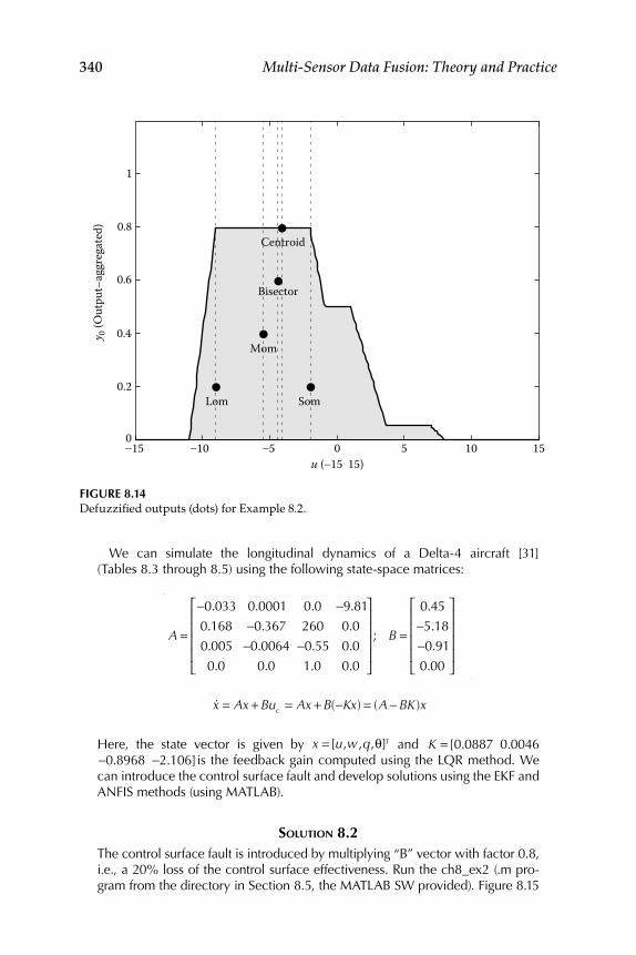
340 Multi-Sensor Data Fusion: Theory and Practice

We can simulate the longitudinal dynamics of a Delta-4 aircraft [31] (Tables 8.3 through 8.5) using the following state-space matrices:

A =

−0.033 0.0001 0.0 −9.81

0.168 −0.367 260 0.0

0.005 −0.0064 −0.55 0.0

0.0 0.0 1.0 0.0

⎡

⎣

⎢⎢⎢⎢

⎤

⎦

⎥⎥⎥⎥; B =

0.45

−5.18

−0.91

0.00

⎡

⎣

⎢⎢⎢⎢

⎤

⎦

⎥⎥⎥⎥

&x = Ax + Buc = Ax + B(−Kx) = (A − BK )x

Here, the state vector is given by x = [u,w ,q,θ]T and K = [0.0887 0.0046 −0.8968 −2.106]is the feedback gain computed using the LQR method. We can introduce the control surface fault and develop solutions using the EKF and ANFIS methods (using MATLAB).

SOLUTION 8.2 The control surface fault is introduced by multiplying “B” vector with factor 0.8, i.e., a 20% loss of the control surface effectiveness. Run the ch8_ex2 (.m pro-gram from the directory in Section 8.5, the MATLAB SW provided). Figure 8.15

FIGURE 8.14 Defuzzifi ed outputs (dots) for Example 8.2.

−15 −10 −5 0 5 10 150

0.2

0.4

0.6

0.8

1

u (−15 15)

y 0 (O

utpu

t–ag

greg

ated

)

Centroid

Bisector

Mom

SomLom

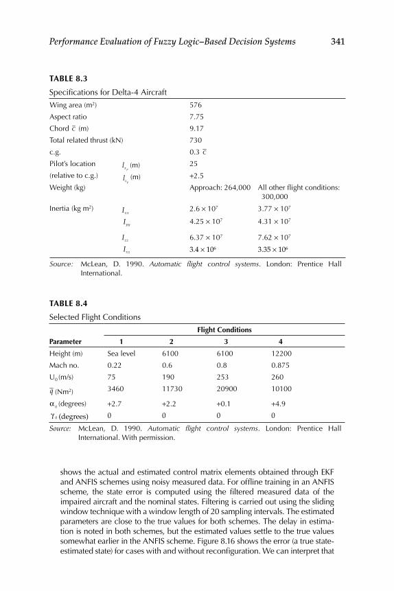
Performance Evaluation of Fuzzy Logic–Based Decision Systems 341

shows the actual and estimated control matrix elements obtained through EKF and ANFIS schemes using noisy measured data. For offl ine training in an ANFIS scheme, the state error is computed using the fi ltered measured data of the impaired aircraft and the nominal states. Filtering is carried out using the sliding window technique with a window length of 20 sampling intervals. The estimated parameters are close to the true values for both schemes. The delay in estima-tion is noted in both schemes, but the estimated values settle to the true values somewhat earlier in the ANFIS scheme. Figure 8.16 shows the error (a true state-estimated state) for cases with and without reconfi guration. We can interpret that

TABLE 8.3

Specifi cations for Delta-4 Aircraft

Wing area (m2) 576

Aspect ratio 7.75

Chord c (m) 9.17

Total related thrust (kN) 730

c.g. 0.3 c

Pilot’s location lx p (m) 25

(relative to c.g.) lz p

(m) +2.5

Weight (kg) Approach: 264,000 All other fl ight conditions: 300,000

Inertia (kg m2) Ixx2.6 × 107 3.77 × 107

Iyy 4.25 × 107 4.31 × 107

Izz 6.37 × 107 7.62 × 107

Ixz 3.4 × 106 3.35 × 106

Source: McLean, D. 1990. Automatic fl ight control systems. London: Prentice Hall International.

TABLE 8.4

Selected Flight Conditions

Parameter

Flight Conditions

1 2 3 4

Height (m) Sea level 6100 6100 12200

Mach no. 0.22 0.6 0.8 0.875

U0 (m/s) 75 190 253 260

q (Nm2) 3460 11730 20900 10100

α0 (degrees) +2.7 +2.2 +0.1 +4.9

γ 0 (degrees) 0 0 0 0

Source: McLean, D. 1990. Automatic fl ight control systems. London: Prentice Hall International. With permission.

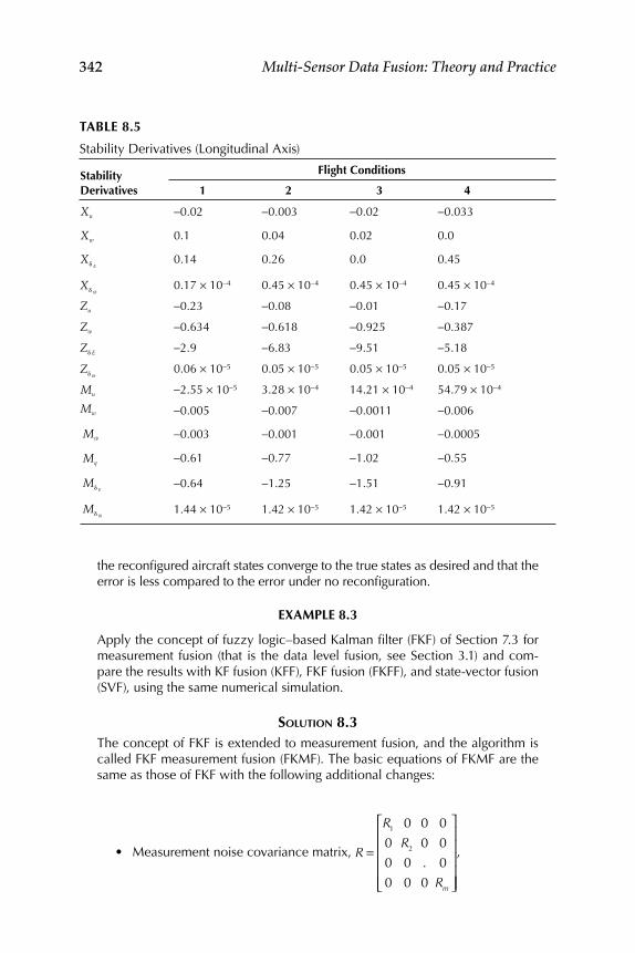
342 Multi-Sensor Data Fusion: Theory and Practice

the reconfi gured aircraft states converge to the true states as desired and that the error is less compared to the error under no reconfi guration.

EXAMPLE 8.3

Apply the concept of fuzzy logic–based Kalman fi lter (FKF) of Section 7.3 for measurement fusion (that is the data level fusion, see Section 3.1) and com-pare the results with KF fusion (KFF), FKF fusion (FKFF), and state-vector fusion (SVF), using the same numerical simulation.

SOLUTION 8.3 The concept of FKF is extended to measurement fusion, and the algorithm is called FKF measurement fusion (FKMF). The basic equations of FKMF are the same as those of FKF with the following additional changes:

Measurement noise covariance matrix, • R =

R1 0 0 0

0 R2 0 0

0 0 . 0

0 0 0 Rm

⎡

⎣

⎢⎢⎢⎢⎢

⎤

⎦

⎥⎥⎥⎥⎥

,

TABLE 8.5

Stability Derivatives (Longitudinal Axis)

Stability Derivatives

Flight Conditions

1 2 3 4

Xu −0.02 −0.003 −0.02 −0.033

Xw 0.1 0.04 0.02 0.0

Xδ E0.14 0.26 0.0 0.45

Xδ th0.17 × 10−4 0.45 × 10−4 0.45 × 10−4 0.45 × 10−4

Zu −0.23 −0.08 −0.01 −0.17

Zw −0.634 −0.618 −0.925 −0.387

Zδ E −2.9 −6.83 −9.51 −5.18

Zδ th0.06 × 10−5 0.05 × 10−5 0.05 × 10−5 0.05 × 10−5

Mu −2.55 × 10−5 3.28 × 10−4 14.21 × 10−4 54.79 × 10−4

Mw −0.005 −0.007 −0.0011 −0.006

M &w −0.003 −0.001 −0.001 −0.0005

Mq −0.61 −0.77 −1.02 −0.55

Mδ E−0.64 −1.25 −1.51 −0.91

Mδ th1.44 × 10−5 1.42 × 10−5 1.42 × 10−5 1.42 × 10−5

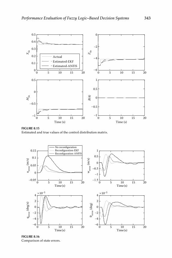
Performance Evaluation of Fuzzy Logic–Based Decision Systems 343

FIGURE 8.15 Estimated and true values of the control distribution matrix.

ActualEstimated-EKFEstimated-ANFIS

0 5 10 15 200

0.1

0.2

0.3

0.4

0.5

X de

0 5 10 15 20-1

-0.5

0

0.5

1

Time (s)

B(4)

0 5 10 15 20-1

-0.5

0

0.5

Time (s)

Mde

0 5 10 15 20-6

-4

-2

0

Z de

FIGURE 8.16 Comparison of state errors.

0 5 10 15 20-6-4-2

024 ´10-3

Time(s)

q erro

r (deg

)

0 5 10 15 20-6-4-2

024 ´10-3

Time(s)

q erro

r (deg

/s)

0 5 10 15 20Time(s)

0 5 10 15 20-0.05

0

0.05

0.1

0.15

Time(s)

u erro

r (m/s

)

-1.5

-0.5

-1

0

0.51

w erro

r (m/s

)

No reconfigurationReconfiguration-EKFReconfiguration-ANFIS

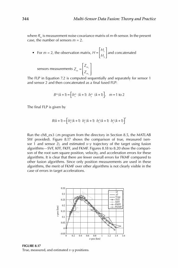
344 Multi-Sensor Data Fusion: Theory and Practice

where Rm is measurement noise covariance matrix of m -th sensor. In the present case, the number of sensors m = 2.

For • m = 2, the observation matrix, H =H1

H2

⎡

⎣⎢

⎤

⎦⎥ and concatenated

sensors measurements Zm =Zm1

Zm2

⎡

⎣⎢⎢

⎤

⎦⎥⎥

The FLP in Equation 7.2 is computed sequentially and separately for sensor 1 and sensor 2 and then concatenated as a fi nal fused FLP:

Bm (k +1) = bm

x (k +1) bmy (k +1)⎡⎣ ⎤⎦ , m = 1 to 2

The fi nal FLP is given by

B(k +1) = bx

1(k +1) by1 (k +1) bx

2(k +1) by2(k +1)⎡⎣ ⎤⎦

T

Run the ch8_ex3 (.m program from the directory in Section 8.5, the MATLAB SW provided). Figure 8.17 shows the comparison of true, measured (sen-sor 1 and sensor 2), and estimated x–y trajectory of the target using fusion algorithms—SVF, KFF, FKFF, and FKMF. Figures 8.18 to 8.20 show the compari-son of the root sum square position, velocity, and acceleration errors for these algorithms. It is clear that there are fewer overall errors for FKMF compared to other fusion algorithms. Since only position measurements are used in these algorithms, the merit of FKMF over other algorithms is not clearly visible in the case of errors in target accelerations.

FIGURE 8.17True, measured, and estimated x–y positions.

0 0.2 0.4 0.6 0.8 1 1.2 1.4 1.6-0.05

0

0.05

0.1

0.15

0.2

0.25

0.3

0.35

x-pos (km)

z-po

s (km

)

s1s2TrueSVFKFFFKFFFKMF

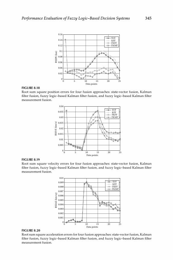
Performance Evaluation of Fuzzy Logic–Based Decision Systems 345

FIGURE 8.18Root sum square position errors for four fusion approaches: state-vector fusion, Kalman

fi lter fusion, fuzzy logic–based Kalman fi lter fusion, and fuzzy logic–based Kalman fi lter

measurement fusion.

0 5 10 15 20 250

0.02

0.04

0.06

0.08

0.1

0.12

0.14

0.16

RSSP

E (k

m)

Data points

SVFKFFFKFFFKMF

FIGURE 8.19Root sum square velocity errors for four fusion approaches: state-vector fusion, Kalman

fi lter fusion, fuzzy logic–based Kalman fi lter fusion, and fuzzy logic–based Kalman fi lter

measurement fusion.

0 5 10 15 20 250

0.005

0.01

0.015

0.02

0.025

0.03

0.035

0.04

RSSV

E (k

m/s

)

Data points

SVFKFFFKFFFKMF

FIGURE 8.20Root sum square acceleration errors for four fusion approaches: state-vector fusion, Kalman

fi lter fusion, fuzzy logic–based Kalman fi lter fusion, and fuzzy logic–based Kalman fi lter

measurement fusion.

0 5 10 15 20 250

0.0010.002

0.0030.0040.005

0.0060.007

0.0080.009

0.01

RSSA

E (k

m/s

2)

Data points

SVFKFFFKFFFKMF

347

Epilogue

Fuzzy logic and systems (FL/S) have been prevalent for four decades and have applications in many engineering systems and household appli-ances. The FL/S discussed in this book are called Type-1 FL/S—Type-0 is the conventional deterministic systems (like defuzzifi ed output of the fuzzy inference system [FIS]/fuzzy control system) and Type-2 FL/S are very recent ideas, and are meant to handle uncertainty in rule-based sys-tems and related developments [32]. Type-1 fuzzy sets are certain, whereas Type-2 FL/S can handle rule uncertainties and even measurement uncer-tainties. In probability theory, the variance provides a measure of dis-persion about the mean [33]. Type-2 FL/S provides a similar measure of dispersion, and linguistic and random uncertainties have a defi nite place in Type-2 FL/S. This new dispersion in Type-2 FL/S can be thought of as being related to a linguistic confi dence interval. A Type-2 FL/S has more degrees of freedom in design than does a Type-1 FL/S and is expected to give a better performance than a Type-1 FL/S. Therefore, new theoretical results and new applications, e.g., data fusion and decision fusion based on Type-2 FL/S, are required.

Exercises

II.1. The fuzzy logic membership function (FLMF) concept is used in KF in Section 7.3 to obtain fuzzy logic (FL)-based KF, via Equations 7.1 to 7.4. This mainly applies to residuals in the KF. Can you think of another approach to using the FLMF concept in KF?

II.2. What is the real reason for checking the consistency of fi lter performance?

II.3. In a crisp representation of the numbers and their sums, differ-ences and equality are governed by fi xed defi nitions. What are the rules for fuzzy members?

II.4. Is it possible to consider a very old man a young boy, and a very young boy an old man? If so, how?

II.5. Why are a domain expert’s knowledge and experience that are needed to build FL-based systems?

348 Multi-Sensor Data Fusion: Theory and Practice

II.6. Why is FL very suitable for decision making and in decision support systems (DM/DSS)?

II.7. Can crisp logic be considered a special case of FL? If so, why?

II.8. Why is defuzzifi cation required in FL/S?

II.9. What is the type in an inner FL system and an output FL system?

II.10. How can FL/S be used for system identifi cation or estimation?

II.11. In Table 6.20, why does the norm of the relational matrices decrease from the standard intersection to the drastic intersection, while the norm increases from the standard union to the drastic union?

II.12. What are the most common forms of fuzzy membership functions?

II.13. What are the two methods of obtaining fuzzy rules (rule bases)?

II.14. What are the features of the two methods in Exercise II.13?

II.15. How can system identifi cation and parameter estimation meth-ods be useful in Exercise II.14?

II.16. When does the conventional control system start to become an intelligent system?

II.17. What are other types of logic in the decision making process?

II.18. What are the features and operators/rules used in these other logics?

II.19. What is the difference between vagueness and uncertainty?

II.20. What is a feedback fuzzy system (FFS)?

II.21. What is the use of FFS?

II.22. Draw an overall block diagram with appropriate elements for modeling a nonlinear system (NLS) with FFS. (Hint: See Figure A.1.)

II.23. What is the meaning of “noise” in the case of the NLS/FFS modeling exercise?

II.24. In what way can the FFS be adjusted for modeling?

II.25. What does “pruning the fuzzy rules” mean and why is it necessary?

II.26. Why do the min and max operators in FL/S have more than one “internal” defi nition, unlike crisp logic, AND, OR, and so on where the results are always unique?

II.27. What is the relationship of decision fusion to data fusion?

II.28. Draw a block diagram for centralized fusion architecture in the case of decision fusion from the classifi er’s point of view.

Performance Evaluation of Fuzzy Logic–Based Decision Systems 349

II.29. How do the decision fusion methods of voting, Bayesian, and Dempster–Shafer compare?

II.30. How do static and dynamic decision making and fusion work?

II.31. It is often said that sensor/decision fusion results are better than would have been possible with only an individual sensor. What is the meaning of “better” here?

II.32. Is the data/decision fusion process the process of “reduction?” How and why?

II.33. Can fuzzy set theory be considered a method of decision fusion?

II.34. Can you visualize the fusion of FL, artifi cial neural networks (ANNs), and genetic algorithms in the context of data fusion itself?

II.35. Changes in the target aspect with respect to the sensor (such as radar or radio frequency-based seekers used in homing missiles to intercept air-breathing targets) can cause the apparent center of sensor refl ections to move from one point to another. This causes noisy or jittered angular measurements. This form of noise is called angle noise, angle scintillations, angle fl uctuations, or glint noise [34,35]. Analysis of the probability density function of glint noise reveals that it has a non-Gaussian, heavy-tailed (due to the spiky pattern of glint noise) distribution. The glint noise can be treated as a mixture of Gaussian noise with moderate vari-ance and a heavy-tailed Laplacian noise with large variance:

pgl int

(w) = (1 − ε)pG (w) + εpL (w)

Here, ε is the “glint probability” and subscripts G and L stand for Gaussian and Laplacian distributions. The probability density functions (pdf’s) of these noises with zero mean are

pL (w) = 1

2ηe− w /η

pG (w) = 1

2π σG

e−w2/2σG2

Here, σG2 is the variance of Gaussian noise and η is related to

Laplacian variance σL2 as 2η2 = σL

2. Within the context of target-track estimation using KF, how would you represent or model glint noise and use it in KF with FL or fuzzy rules? Give the important steps.

350 Multi-Sensor Data Fusion: Theory and Practice

II.36. ANNs are biologically inspired, with abilities to learn and adapt (see Figure A.6) due to (1) perception, (2) multilayer feed-forward networks, (3) recurrent networks, and (4) a radial basis function (RBF) neural network. The RBF network is characterized by radial basis functions. An RBF network has good local interpolation, global generalization ability, and is more biologically plausible because of its fi nite response. Also, it can initially have zero neu-rons in a hidden layer, and online neurons can be created and pruned. One such RBF network is known as minimum resource allocation network (MRAN) [35,36]. MRAN has been used in sev-eral applications varying from function approximation to non-linear system identifi cation and its application in fl ight control. A topology of RBF neural networks with Gaussian functions (as a type of radial basis function), which can be easily used for data fusion (Exercise III.7), is shown below [36,37]. The RBF neural net-work response at each of its output node is given by

yk = bk + αkjφ j (U)j=1

n

∑ ; k = 1,..., p

φ j (U) = exp− U − μ j

σ j2

⎛

⎝⎜⎜

⎞

⎠⎟⎟

where U = [u

1, ..., um ] is the input vector to network and ⏐⏐.⏐⏐

denotes the Euclidean norm. Simulate the following nonlinear function having six Gaussian functions using MRAN [35,36]:

y(x) = exp −(x

1− 0.3)2 + (x

2− 0.2)2

0.01

⎡

⎣⎢

⎤

⎦⎥ + exp −

(x1

− 0.7)2 + (x2

− 0.2)2

0.01

⎡

⎣⎢

⎤

⎦⎥

+ exp −(x

1− 0.3)2 + (x

2− 0.8)2

0.01

⎡

⎣⎢

⎤

⎦⎥ + exp −

(x1

− 0.7)2 + (x2

− 0.8)2

0.01

⎡

⎣⎢

⎤

⎦⎥

+ exp −(x

1− 0.1)2 + (x

2− 0.5)2

0.02

⎡

⎣⎢

⎤

⎦⎥ + exp −

(x1

− 0.9)2 + (x2

− 0.5)2

0.02

⎡

⎣⎢

⎤

⎦⎥

II.37. Why does the FL–based KF (FLKF) generally not meet the fi lter-consistency check as accurately as the standard KF?

II.38. Why is decision making in KF called soft decision making?

II.39. What type of decision making is used in FLKF?

II.40. What kind of fusion processes can be used for data that are not homogeneous quantities?

Performance Evaluation of Fuzzy Logic–Based Decision Systems 351

II.41. What is the major difference between the forward- and backward-chaining inference rules?

II.42. Is it possible to combine FL and the Bayesian method for data fusion or decision fusion?

II.43. Can you visualize a decision fusion strategy?

II.44. Is it possible to combine FL, a genetic algorithm, and ANN to form a decision fusion system?

II.45. Is it possible to use FL for image fusion?

II.46. What are the strong and weak aspects of FL for fusion?

II.47. In what way can the combination of FL, ANN, and KF be used to track a maneuvering target?

II.48. How one can apply the FL, FMF, or FIS process to image pro-cessing or fusion?

II.49. Is there any mapping involved in the use of FL/FIS to design a fusion system based on FL? Is this mapping linear or nonlinear?

II.50. What does FL represent in the case of noisy sensors used for tracking/data fusion, since the noise is already represented by the Gaussian probability density function (pdf) with often a zero mean and a given standard deviation?

II.51. In Chapter 6, while discussing FL operators and their intercon-nectivity, we came across conjunction and disjunction Cartesian products. Can you discuss these in terms of the fusion process?

II.52. How can FL be used for data classifi cation? What are the differ-ent clustering techniques available for classifi cation?

References

1. Zadeh, L. A. 1965. Fuzzy sets. Inf Control 8:338–53. 2. King, R. E. 1999. Computational intelligence in control engineering . New York:

Marcel Dekker. 3. Passino, K. M., and S. Yurkovich. 1998. Fuzzy control . Menlo Park, CA:

Addison-Wesley Longman. 4. Kosko, B. 1997. Fuzzy engineering . Upper Saddle River, NJ: Prentice Hall. 5. Kashyap, S. K., J. R. Raol, and A. V. Patel. 2008. Evaluation of fuzzy implica-

tions and intuitive criteria of GMP and GMT. In Foundations of generic optimi-zation, Vol. 2: Applications of fuzzy control, genetic algorithms and neural networks ( Mathematical modelling: Theory and applications ), pp. 313–386, ed. R. Lowen and A. Verschoren. New York: Springer.

352 Multi-Sensor Data Fusion: Theory and Practice

6. Kashyap, S. K., and J. R. Raol. 2007. Interpretation and unifi cation of fuzzy set operations and implications. J Syst Soc India 16(1):26–33.

7. Kashyap, S. K. 2008. Decision fusion using fuzzy logic. Doctoral thesis, University of Mysore, Mysore, India.

8. Li-Xin, W. 1994. Adaptive fuzzy systems and control, design and stability analysis . Englewood Cliffs, NJ: Prentice Hall.

9. Raol, J. R., and J. Singh. 2009. Flight mechanics modeling and analysis . Boca Raton, FL: CRC Press.

10. Cho, S. B., and J. H. Kim. 1995. Multiple network fusion using fuzzy logic. IEEE Trans Neural Netw 6(2):497–501.

11. Lau, C. W., B. Ma, H. M. Meng, Y. S. Moon, and Y. Yam. 2004. Fuzzy logic decision fusion in a multimodal biometric system. http://www.se.cuhk.edu.hk/hccl/publications/pub/lau_icslp2004.pdf (accessed December 2008).

12. Wik, M. W. 2006. A three processes effects model based on the meaning of information. 11th ICCRTS Coalition Command and Control in the Networked Era, September 26–28, 2006. http://www.dodccrp.org/events/11th_ICCRTS/html/presentations/018.pdf (accessed December 2008).

13. Crowley, J. L., and Y. Demazeu. 1993. Principles and techniques of sensor data fusion. LIFIA (IMAG), France. http://www-prima.imag.fr/Prima/Homepages/jlc/papers/SigProc-Fusion.pdf (accessed July 2008).

14. Kant, E. 1958. Critique of pure reason, translated by N. Kemp Smith. New York: Random House (original work published in 1781).

15 Abidi, M. A., and R. C. Gonzalez, eds. 1992. Data fusion in robotics and machine intelligence . USA: Academic Press.

16. Hall, D. L. 1992. Mathematical techniques in multi-sensor data fusion . Norwood, MA: Artech House.

17. Chao, W., Q. Jishuang, and L. Zhi. Data fusion, the core technology for future on-board data processing system. Institute of Remote Sensing Applications, Chinese Academy of Sciences, Beijing, China.

18. Klein, L. A. 2004. Sensor and data fusion: A tool for information assessment and decision making . Washington, DC: SPIE Press.

19. Egfi n Nirmala, D., V. Vaidehi, S. Indira Gandhi. 2005. Data fusion using fuzzy logic for multi target tracking. In Proceedings of International Radar Symposium India, pp. 75–80.

20. Kashyap, S. K., and J. R. Raol. 2008. Fuzzy logic applications for fi ltering and fusion for target tracking. Def Sci J 58:120–35.

21. Ivansson, J. 2002. Situation assessment in a stochastic environment using Bayesian networks. Master’s thesis, Division of Automatic Control, Department of Electrical Engineering, Linkoping University.

22. Narayana Rao, P., S. K. Kashyap, and G. Girija. 2008. Situation assessment in air combat: A fuzzy-Bayesian hybrid approach. In Proceedings of the International Conference on Aerospace Science and Technology, NAL, Bangalore, India.

23. Endsley, M. R. 1993. A survey of situation awareness requirements in air-to-air combat fi ghters. Int J Aviat Psychol 3:157–68.

24. Neapolitan, R. E. 1990. Probabilistic reasoning in expert systems . New York: John Wiley & Sons.

Performance Evaluation of Fuzzy Logic–Based Decision Systems 353

25. Pearl, J. 1988. Probabilistic reasoning in intelligent systems: Networks of plausible inference. San Francisco, CA: Morgan Kaufmann Publishers, Inc.

26. HUGIN Expert, http//: www.HUGIN.dk (accessed December 2008). 27. Hajiyev, Ch. M., and F. Caliskan. 2001. Integrated sensor/actuator FDI and

reconfi gurable control for fault tolerant fl ight control system design. Aeronaut J 105:525–33.

28. Hajiyev, C., and F. Caliskan. 2003. Fault diagnosis and reconfi guration in fl ight control systems . Boston: Kluwer Academic Publishers.

29. Eva Wu, N., Y. Zhang, and K. Zhou. 2000. Detection, estimation, and accommodation of loss of control effectiveness. Int J Adapt Control Process 14:775–95.

30. Savanur, S. R., S. K. Kashyap, and J. R. Raol. 2008. Adaptive Neuro-Fuzzy based control surface fault detection and reconfi guration. In Proceedings of the International Conference on Aerospace Science and Technology, Bangalore, India.

31. McLean, D. 1990. Automatic fl ight control systems . London: Prentice Hall International.

32. Mendel, J. M. Why we need Type-2 fuzzy logic system. http://www.informit.com/articles/article.aspx?p=21312-32k (accessed January 2009).

33. Raol, J. R., G. Girija, and J. Singh. 2004. Modelling and parameter estimation of dynamic systems, IEE Control Engineering. Series Book . Vol. 65. London: IEE.

34. Hewer, G. A., R. D. Martin, and J. Zeh. 1987. Robust preprocessing for Kalman fi ltering of glint noise. IEEE Trans Aerosp Electron Syst 23:120–8.

35. Wu, W. 1993. Target tracking with glint noise. IEEE Trans Aerosp Electron Syst 29:174–85.

36. Sundararajan, N., P. Saratchandran, and Y. W. Lu. 2001. Radial basis function neural networks with sequential learning—MRAN and its applications, Progress in neural processing 11 . Singapore: World Scientifi c Publishing.

37. Lu, Y., N. Sundararajan, and P. Saratchandran. 1997. A sequential learning scheme for function approximation using minimal radial basis function neu-ral networks. Neural Comput 9:461–78.

III Part

Pixel- and Feature-Level Image Fusion

J. R. Raol and V. P. S. Naidu

357

9 Introduction

We work with visual images every day of our lives. We recognize static and moving objects naturally and promptly. We teach our children by showing them line diagrams, pictures, and images. We give these images names and ask our children to recognize the objects and give their names. Our daily lives are a world of pictures, 2D and 3D images, and sounds. Our biological neural networks instantaneously recognize these images and, when required, quickly perform fusion of the images. One of our basic needs in evolution has been the recognition, registration, and fusion of the images we encounter daily, even every second or milli second. Our imaging system is based on the ability to see light-illuminated objects. However, in the technological world many other methods of imaging are available: laser, nuclear magnetic resonance, and infrared (IR). We live in an environment of images and sounds. We have an uncanny ability to recognize and relate human faces—in far away places, we often say that the face of a person is similar to the face of someone whom we have seen earlier, and we can even see the faces and features of persons and objects (including animals, birds, and insects) in the clouds, and profi les in the silhouettes of mountains!

Image fusion is the process of combining information from two or more sensed or acquired images into a single composite image that is more infor-mative and more suitable for visual perception and computer or visual processing. The objective is to reduce uncertainty, minimize redundancy in the output, and maximize relevant information pertaining to an appli-cation or a task. For example, if a visual image is fused with a thermal image, a target that is warmer or colder than its background can be eas-ily identifi ed, even when its color and spatial details are similar to those of its background. In image fusion, the image data appear in the form of arrays of numbers, which represent brightness (intensity), color, tempera-ture, distance, and other scene properties. These data could be 2D or 3D. The 3D data are essentially the volumetric images and/or video sequences in the form of spatial-temporal volumes. The approaches for image fusion are (1) hierarchical image decomposition, (2) neural networks in fusion of visible and IR images, (3) laser detection and ranging (LADAR) and passive IR images for target segmentation, (4) discrete wavelet transforms (DWTs), (5) principal component analysis (PCA), and (6) principal compo-nents substitution (PCS).

358 Multi-Sensor Data Fusion: Theory and Practice

Image fusion can be categorized as of the following [1–4]:

1. Low-level: Pixel-level fusion is done in the spatial or transform domain (TD). TD algorithms globally create the fused image. The algorithms that work in the spatial domain have the ability to focus on desired image areas, limiting changes in other areas. Multi-resolution analysis can use fi lters with increasing spatial extent to generate a sequence of images (pyramids) from each image, sepa-rating the information observed at different resolutions. Then, at each position in the transformed image, the value in the pyramid showing the highest saliency is taken. An inverse transform of the composite image is used to create the fused image. Intensity gradients can be used as saliency measures. Dual-tree complex wavelet transform can outperform most other grayscale image fusion methods.

2. Mid-level: Feature-level fusion algorithms typically segment the images into regions and fuse the regions using their various properties. The multiscale edge representations using wavelet transform can also be used for image fusion.

3. High-level: Symbol-level fusion algorithms combine image descriptions in the form of relational graphs. Since decision fusion and symbol-level fusion are very closely related, fuzzy logic theory can also be used for this level of fusion.

In pixel-level fusion, there are three broad approaches: (1) color transfor-mation (CT), (2) statistical and numerical (SN), and (3) multiresolution method (MRM). In the CT method, there is an advantage in the possibility of presenting the data in different color channels, including hue (H, domi-nant wavelength), intensity (I), and saturation (S; called HIS approach). The red, green, and blue (RGB) image is divided into spatial (I) and spectral (H and S) information. There are two kinds of possible transformations: (1) transform the three images (channels) presented in RGB into I, H, and S directly; and (2) separate the color channels into average brightness rep-resenting the surface roughness (intensity), dominant wavelength (hue), and purity (saturation). The HIS approach has become standard proce-dure in image analysis. It has the ability to enhance the color of highly correlated data and can fuse disparate data.

In the SN method, the PCA utilizes all channels’ data as input and com-bines the multisensor data into one major part. The PCS regards one chan-nel’s data as a major part at fi rst, and then substitutes it with the other channel’s data if it has a better fused result. These methods do not pre-serve the spectral characteristics of the source image well, since the fused image features will be altered to a great extent.

Introduction 359

The MRM method is preferable (as are the pyramid-based and wavelet-based methods). The Gaussian pyramid and enhanced Laplacian (ELP) decomposition can only decompose and interpolate images with a decimation factor of 2, resulting in many restrictions. Laplacian pyra-mids correspond to a band-pass representation, while Gaussian pyramids correspond to a low-pass representation. Pyramids are an example of a wavelet representation of an image and correspond to the decompo-sition of an image into spatial/frequency bands. The wavelets separate information into frequency bands; in the case of images we present high- frequency information, such as texture and so forth, in a fi nely sampled grid [5]. Coarse information can be represented in a coarser grid where the lower sampling rate is acceptable. Coarse features can be detected in the coarse grid using a small template size (this is referred to as multireso-lution or multiscale resolution ). Wavelets correspond to a mixture of spatial and frequency domains; the position information at each level is known to the accuracy of that grid resolution and contributing frequencies are bandwidth limited at each grid resolution. Since wavelet coeffi cients that have large absolute values contain information about the salient features of images, such as edges and lines, a good rule is to take the maximum absolute values of the corresponding wavelet coeffi cients. The maximum absolute value, within a window, is used as an activity measure of the central pixel of the window. In the wavelet fusion method, the trans-formed images are combined in the transform domain using a defi ned fusion rule and then transformed back to the spatial domain to obtain the fused image. The wavelet package (WP)–based method uses a WP to further decompose multitemporal images at low- or high-frequency parts. At the same level, it utilizes a threshold and weight algorithm to fuse the corresponding low-frequency parts, and at the same time applies a Lis high-pass fi lter to fuse the high frequency parts. The fused image is then restored by inverse DWT process. The WT package fusion method [6] decomposes the image recursively at fi rst, which means decomposing the low-frequency part of the previous level. Let the grayscale image after decomposition by WT be Io. Then

Io = base image (approximations) + vertical + horizontal + diagonal details

The base image is decomposed at the second level and so on, thus, the n th decomposition will comprise 3 n + 1 subimage sequences. The 3 n + 1 subimage sequences of the n th level will be fused by applying different rules to low- and high-frequency parts. Then the inverse WT is taken to restore the fused image. The WP method decomposes every part of the previous level recursively, to either low frequency or high frequency; thus there will be 4-power n subimage sequences at the n th decomposition,

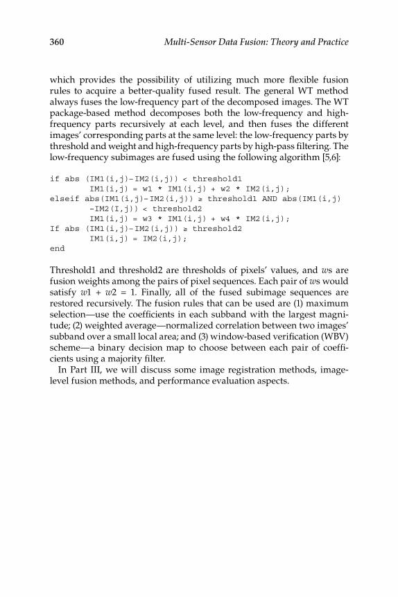
360 Multi-Sensor Data Fusion: Theory and Practice

which provides the possibility of utilizing much more fl exible fusion rules to acquire a better-quality fused result. The general WT method always fuses the low-frequency part of the decomposed images. The WT package-based method decomposes both the low-frequency and high- frequency parts recursively at each level, and then fuses the different images’ corresponding parts at the same level: the low-frequency parts by threshold and weight and high-frequency parts by high-pass fi ltering. The low-frequency sub images are fused using the following algorithm [5,6]:

if abs (IM1(i,j)–IM2(i,j)) < threshold1 IM1(i,j) = w1 * IM1(i,j) + w2 * IM2(i,j); elseif abs(IM1(i,j)–IM2(i,j)) ≥ threshold1 AND abs(IM1(i,j) –IM2(I,j)) < threshold2 IM1(i,j) = w3 * IM1(i,j) + w4 * IM2(i,j); If abs (IM1(i,j)–IM2(i,j)) ≥ threshold2 IM1(i,j) = IM2(i,j); end

Threshold1 and threshold2 are thresholds of pixels’ values, and w s are fusion weights among the pairs of pixel sequences. Each pair of w s would satisfy w 1 + w 2 = 1. Finally, all of the fused subimage sequences are restored recursively. The fusion rules that can be used are (1) maximum selection—use the coeffi cients in each subband with the largest magni-tude; (2) weighted average—normalized correlation between two images’ subband over a small local area; and (3) window-based verifi cation (WBV) scheme—a binary decision map to choose between each pair of coeffi -cients using a majority fi lter.

In Part III, we will discuss some image registration methods, image-level fusion methods, and performance evaluation aspects.

361

10 Pixel- and Feature-Level Image Fusion Concepts and Algorithms

The data or information fusion process can take place at different levels, such as the signal, pixel, feature, and symbolic levels. Signal-level process-ing and data fusion have been discussed in Part I. In Part II, we discussed some aspects of decision fusion based on fuzzy logic. In the pixel-level fusion process, a composite image is built from several input images based on their respective pixels (picture elements). One of the applications is the fusion of forward-looking infrared (FLIR) and low-light visible images (LLTV) obtained by an airborne sensor system to aid the pilot navigate in poor weather conditions and darkness. In pixel-level fusion, some basic aspects of the fusion result are as follows [7–10]: (1) the data fusion (DF) process should carry over all the useful and relevant information from the input images to the composite image, to the greatest extent possible; (2) the DF scheme should not introduce any additional inconsistencies not originally present in the input images, which would distract the observer or other subsequent processing stages; and (3) the DF process should be shift and rotational invariant. The fusion results should not depend on the location or orientation of an object from the input images. Addition-ally, there should be (1) temporal stability, that is, the gray level changes in the fused image sequence should only be caused by gray level changes in the input sequences, and not by the fusion process; and (2) temporal consistency, that is, gray level changes occurring in the input image sequences should be present in the fused image sequence without any delay or contrast change.

10.1 Image Registration

In the image registration process, two (or more) sensed images of the same scene are superimposed [1–4]. These images might have been taken at different times, from different viewpoints, or from different sensors. The main idea is to geometrically align the sensed image and the reference image. Certain differences in images of the same scene

362 Multi-Sensor Data Fusion: Theory and Practice

might arise due to differing imaging conditions. Image registration is required for several applications: (1) multispectral classifi cation, (2) environmental monitoring, (3) change detection, (4) image mosaic, (5) weather forecasting, (6) creating super-resolution images, (7) integrat-ing information into geographical information systems, (8) combining computer tomography and nuclear magnetic resonance (NMR) data, (9) map updating (cartography), (10) target localization, and (11) auto-matic quality control. The image registration applications can be divided into four groups [3]:

1. Multiview analysis: Images of the same scene are acquired from different viewpoints in order to obtain a larger 2D or 3D representation of the observed scene. The examples are image mosaics of the surveyed area and shape recovery from stereo.

2. Multitemporal analysis: Images of the same scene are acquired at different times in order to fi nd and evaluate changes in the scene that appeared in the time between the acquisition of the images. This includes monitoring global land usage, landscape planning, automatic change detection for security monitoring, motion tracking, monitoring of healing therapy, and monitoring tumor growth.

3. Multimodal analysis: Images of the same scene are acquired by different sensors in order to integrate the information obtained from the different sources to obtain a more complex and detailed scene representation. Examples include the fusion of information from sensors with different characteristics, such as panchromatic images, images offering a better spatial resolution, color/multi-spectral images with a better spectral resolution, radar images independent of cloud cover and solar illumination. Also included are combinations of sensors recording the anatomical body structure, such as magnetic resonance image (MRI), ultrasound or CT scans, and sensors monitoring functional and metabolic body activities, like positron emission tomography (PET), single photon emission computed tomography (SPECT), and magnetic resonance spectroscopy (MRS).

4. Scene to model registration: Images of a scene and a model of the scene are registered. The model could be maps or digital eleva-tion models in a geographic information system (GIS), another scene with similar content, or an average specimen. The aim is to localize the acquired images in the scene or model and com-pare them. Some examples are the registration of aerial or satellite data onto maps or other GIS layers, target template matching with real-time images, automatic quality inspection, comparison of the

Pixel- and Feature-Level Image Fusion Concepts and Algorithms 363

patient’s image with digital anatomical atlases, and specimen classifi cation.

Low-level fusion algorithms assume there is a correspondence between pixels in the input images. If the camera’s intrinsic and extrinsic parameters (IEPs) do not change and only the environmental parameters change, then the acquired images will be spatially registered. When the IEPs are dif-ferent, the registration of images is required. Mid-level fusion algorithms assume that the correspondence between the features in the images is known. High-level fusion algorithms require correspondence between image descriptions for comparison and fusion.

Although the most common method of image registration is to man-ually align the images (which is time consuming and inaccurate), there are two main approaches: (1) area-based matching (ABM), and (2) fea-ture-based matching (FBM). In the registration method, it is important to fi nd enough accurate control input pairs and a procedure to interpolate the image. Any image registration method should take into account the assumed type of geometric deformation between the images, radiomet-ric deformations, noise corruption, required registration accuracy, and application-dependent data characteristics. The main registration methods follow these steps:

1. Feature detection: Salient objects such as regions, edges, contours, and corners are detected. These features are represented by their center of gravity (CG) and end points.

2. Feature matching: The correspondence between the observed image and the reference image is ascertained. Various feature descriptors and spatial relationships are used for this purpose.

3. Transform model estimation: The parameters of the mapping functions are determined based on the feature correspondence.

4. Image resampling and transformation: The image is transformed using mapping functions.

10.1.1 Area-Based Matching

The detected features in the two images (the reference image and the sensed image) can be matched using the image intensity values in their close neighborhoods, spatial distribution, or the symbolic representation for feature matching.

ABM is also called the correlation-like or template-matching method [3].This method merges feature detection with matching and does not attempt to detect salient objects. Windows of a predetermined size are used for correspondence estimation. In this classical method, a small rectangular

364 Multi-Sensor Data Fusion: Theory and Practice

or circular window of pixels in the image is compared statistically with windows of the same size as the reference image. The centers of the matched windows are treated as control inputs. These are used to solve for mapping function parameters between the reference image and the sensed image. The cross-correlation methods use matching of the intensities directly, and do not bother with the structural analysis. The normalized cross-correlation (NCC) and least-squares (LS) techniques are also widely used for this purpose. NCC is based on the maximum value of the cor-relation coeffi cient between the reference image and the sensed image. LS is based on minimizing the differences in the gray values between the reference image and the sensed image. The area correlation in the spatial domain can be used to match the feature points. These points are extracted by Gabor wavelet decomposition.

10.1.1.1 Correlation Method

The correlation method is based on normalized correlation, defi ned as follows:

CC(i, j) =w − E(w)( ) I(i, j) − E I(i, j)( )⎛

⎝⎜⎞⎠⎟∑

w − E(w)( )2∑ I(i, j) − E I(i, j)( )⎛⎝⎜

⎞⎠⎟

2

∑ (10.1)

The CC value is computed for window pairs from the sensed and reference images. The maximum of CC is sought. For subpixel accuracy, the inter-polation of CC values is used. Correlation-based methods are still being used because of their ease in the hardware implementation and hence are useful in real-time applications. Feature points can be detected using a wavelet transform (WT) algorithm, and then the cross-correlation method can be used to match the detected points across the images. Often, ABM is used to fi nd the similarity of the features in the reference and sensed images.

10.1.1.2 Fourier Method

The Fourier representation of the images in the frequency domain is used in this method. The Fourier method computes the cross-power spectrum of the sensed and reference images, seeking the location of the peak in its inverse. This method is very robust in the presence of the correlated noise and the frequency dependent noise. This ABM can be effectively implemented in the fast Fourier transform (FFT) domain. Some of the FFT can be used to achieve invariance to translation, rotation, and scale. These ABM algorithms are easy to implement because of their simple mathe-matical models.

Pixel- and Feature-Level Image Fusion Concepts and Algorithms 365

10.1.1.3 Mutual Information Method

The mutual information (MI) method is a leading method in multimodal registration, especially in medical imaging. For example, a compari-son of the anatomical and functional images of the body of the patient would lead to a useful diagnosis. Another useful application is the area of remote sensing (discussed in Section 2.4). The main idea is to maximize the MI. Here, the various possibilities include the use of joint entropy, the MI, and the normalized MI. In this approach, all of the image data and image intensities are used. An optimization method might be required for maximization of the MI.

10.1.2 Feature-Based Methods

FBMs use the image features (the salient structures in the image), derived by a feature extraction algorithm [1–3]. Usually, the features include edges, contours, surfaces, corners, line intersections, and points, for example: (1) signifi cant regions such as forests, fi elds, lakes, and ponds; (2) signifi cant lines in region boundaries, coastlines, roads, and rivers; and (3) signifi cant points in region corners, line intersections, and points on curves with high curvatures. The features should be distinct and should be spread all over the image. First, these features should be effi ciently detectable in both of the images that are being compared, and they should also be stable at fi xed positions, otherwise a comparison cannot be correctly made. The number of common elements in the detected sets of the features should be very high. FBMs do not work directly with the values of image intensity. Sta-tistical features such as moment invariants or centroids and higher level structural and syntactic descriptions are also used. FBMs can be used for feature detection and feature matching. The various approaches in FBMs are as follows:

1. Use of the corresponding centers of gravity of regions as cor-responding control points (CPs) to estimate the registration parameters; these centers of gravity should be invariant with the rotation, scaling, and skewing of the corresponding images. They should also be stable, even in the presence of noise and variation in gray levels. The region features are detected using segmenta-tion methods.

2. Use of structural similarity detection techniques.

3. Use of the affi ne moment invariants principle, a segmentation technique, in registering an image with an affi ne geometric distortion.

4. Use of contour-based methods that use regional boundaries and other strong edges as matching primitives.

366 Multi-Sensor Data Fusion: Theory and Practice

5. Use of a combined invariant moment shape descriptor and improved chain-code matching to establish correspondence between potentially matched regions detected in two images.

6. Use of line segments as primitive in a registration process. Line features are object contours, coastal lines, and roads. The corre-spondence of lines is expressed by pairs of line ends.

7. Use of wavelet decomposition for generating the pyramidal struc-ture, because of its multiresolution characteristics.

8. Use of Gabor WT decomposition to extract feature points.

9. Use of local modulus maxima of the WT to fi nd feature points and the cross-correlation method to build correspondence between these feature points.

10. Use of maximum of WT coeffi cients to form the basic features of a correlation-based automatic registration algorithm.

To apply FBMs for feature matching, it is assumed that the two sets of fea-tures in the two images under the test are detected. The goal is to fi nd pair-wise relationships between these features using spatial correspondences or other descriptions of the detected features.

10.1.2.1 Spatial Relation

Information about the distances between the CPs (such as line endings, distinctive points, and centers of gravity) and their spatial distributions is used in this method of feature matching. The methods are (1) graph matching—a number of features are evaluated, and after a particular transformation they fall within a given range next to the features in the reference image; the transformation parameters with the highest scores are used; (2) clustering method—using the points connected by abstract edges and line segments, the cluster is detected; its centroid represents the most probable vector of matching parameters; and (3) chamfer matching—line features in the images are matched using the minimization of the general-ized distance between them.

10.1.2.2 Invariant Descriptors

A correspondence between the features from the two images is deter-mined using invariant descriptors of these features [3]. The descriptors should be invariant, unique, stable, and independent. Often a trade-off amongst these requirements might be necessary. The most invariant descriptors from the two images are paired. The simplest descriptor is the image intensity function itself. For matching CC, any distance or MI criteria can be used.

Pixel- and Feature-Level Image Fusion Concepts and Algorithms 367

A wild forest, for example, can be described by elongation parame-ters, compactness, number of holes, and so on. A detected feature can be represented by its signature, for example, the longest structure and the angles between the remaining structures. The closed-boundary regions can also be used as features. The invariant descriptors can be defi ned as radial-shaped vectors, polygons, moment-based, perimeters, areas, com-pactness, extracted contours and slopes of the tangents in the contours, histograms of line ratios, histograms of angle differences, ellepticity, angle, thinness, and so on.

10.1.2.3 Relaxation Technique

This technique is part of solution to the consistent labeling problem. The idea is to label each feature from the sensed image with the label of a fea-ture from the reference image. This method can be enhanced by a descrip-tor approach using corner sharpness, contrast, slope, and so on.

10.1.2.4 Pyramids and Wavelets

It is often necessary to attempt to reduce the computational burden asso-ciated with the registration techniques and algorithms. We can use the subwindow to minimize the computational cost. We can start with a coarser-resolution grid and then proceed to higher- resolution grids, or use the sparse regular grid of windows and perform cross- correlation and related methods. The foregoing are the simple examples of the pyra-midal techniques [3–6]. The point is to start with the coarser grids or windows and proceed step by step to fi ner grids in a hierarchical manner for feature matching. We can use Gaussian pyramids, simple averaging, or wavelets for obtaining a coarse resolution in the fi rst place. Then, sys-tematically and gradually, the estimates of the parameters of the map-ping functions or the correspondence are improved, while leading to a fi ner resolution, thereby monitoring and controlling the computational cost, desired resolution, and accuracy of feature matching. The major aspect of the initial feature matching would have already been obtained using the coarse-resolution grids, and then the fi ner matching can be carried out, if required, for the fi ner details. However, the consistency should be checked to avoid false matching, using the coarser grid or win-dow. We can use concepts of median pyramid and averaging pyramid based on the process applied to the number of pixels. Wavelet decompo-sition can also be used in the pyramidal approach using the orthogonal or biorthogonal wavelets for multiresolution analysis. The main idea is to use the wavelet coeffi cients of the two images and seek correspon-dences between the features from the two images in terms of the impor-tant coeffi cients.

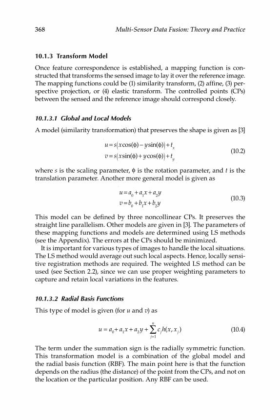
368 Multi-Sensor Data Fusion: Theory and Practice

10.1.3 Transform Model

Once feature correspondence is established, a mapping function is con-structed that transforms the sensed image to lay it over the reference image. The mapping functions could be (1) similarity transform, (2) affi ne, (3) per-spective projection, or (4) elastic transform. The controlled points (CPs) between the sensed and the reference image should correspond closely.

10.1.3.1 Global and Local Models

A model (similarity tran s formation) that preserves the shape is given as [3]

u = s xcos(φ) − ysin(φ)( ) + tx

v = s xsin(φ)+ ycos(φ)( ) + ty

(10.2)

where s is the scaling parameter, φ is the rotation parameter, and t is the translation parameter. Another more general model is given as

u = a0

+ a1x + a

2y

v = b0

+ b1x + b

2y

(10.3)

This model can be defi ned by three noncollinear CPs. It preserves the straight line parallelism. Other models are given in [3]. The parameters of these mapping functions and models are determined using LS methods (see the Appendix). The errors at the CPs should be minimized.

It is important for various types of images to handle the local situations. The LS method would average out such local aspects. Hence, locally sensi-tive registration methods are required. The weighted LS method can be used (see Section 2.2), since we can use proper weighting parameters to capture and retain local variations in the features.

10.1.3.2 Radial Basis Functions

This type of model is given (for u and v ) as

u = a

0+ a

1x + a

2y + cjh(x, xj )

j=1

n

∑ (10.4)

The term under the summation sign is the radially symmetric function. This transformation model is a combination of the global model and the radial basis function (RBF). The main point here is that the function depends on the radius (the distance) of the point from the CPs, and not on the location or the particular position. Any RBF can be used.

Pixel- and Feature-Level Image Fusion Concepts and Algorithms 369

10.1.3.3 Elastic Registration

The idea in elastic registration is not to use any parametric mapping function. In this approach, the images are regarded as pieces of rubber or elastic sheets [3]. Here, the external and internal forces to stretch the image or make it stiff are brought into play. Image registration is per-formed by achieving the minimum energy state in an iterative manner. However, some similarity functions are needed to defi ne the forces. These functions again depend on the intensity values and the correspondence of the boundary structures. We can use the fl uid registration approach or the diffusion-based registration approach. Due to the possibility of various types of elastic models, there is an immense scope of development of new and effi cient image registration methods within the precincts of the elastic registration methods.

10.1.4 Resampling and Transformation

For the purpose of transformation, each pixel from the sensed image is transformed using the estimated mapping functions. Another approach is to determine the registered image data from the sensed image data using the coordinates of the target pixel and the inverse of the estimated mapping function. The coordinate system used is the same as that of the reference image. The image interpolation that takes place in the sensed image on the regular grid is realized via convolution of the image with an interpolation kernel. For interpolation, we can use any of the following functions: (1) bilinear, (2) nearest neighbor, (3) splines, (4) Gaussians, and (5) sinc functions.

10.1.5 Image Registration Accuracy

There are several types of errors that can occur during the process of image registration [3]: (1) localization errors, (2) matching errors, and (3) alignment errors. Localization errors occur due to the displacement of the CP coordinates which in turn is due to their inaccurate detection. These errors can be reduced using an optimal feature detection algorithm. Matching errors indicate the number of false matches in the correspon-dence of the CPs of both the images. We can use the consistency check or the cross-validation to identify the false matches. Alignment errors are the difference between the mapping model and the actual between-image geometric distortion. Alignment errors can be assessed using another comparative method. Visual assessment by a domain expert is still used as a complementary method to objective error evaluation methods.

370 Multi-Sensor Data Fusion: Theory and Practice

10.2 Segmentation, Centroid Detection, and

Target Tracking with Image Data

Tracking moving objects or targets using image data involves processing images and producing an estimate of the object’s current position and velocity vectors at each step. There is additional uncertainty regarding the origin of the received data, which may or may not include measurements from the targets. This may be due to random clutter (false alarms). This data association problem was addressed in Chapter 3. In this section, the focus is on the use of the algorithm for tracking with segmentation from imaging sensors [7,11]. This centroid detection and tracking (CDT) algorithm is inde-pendent of the size of targets and is less sensitive to the intensity of the tar-gets. The typical characteristics of the target obtained by motion- recognition or object/pattern-recognition are used to associate images with the target being tracked. The motion recognition characteristics location, velocity, and acceleration (as a total state vector) are generated using data from successive frames (interscan level), whereas the object/pattern-recognition characteris-tics, geometric structure such as shape and size, and energy levels (different gray levels in the image) in one or more spectral bands are obtained using image data at the intrascan level. The CDT algorithm combines both object- and motion-recognition methods for target tracking from imaging sensors. The properties of the image considered are the intensity and size of the clus-ter. The pixel intensity is discretized into layers of gray level intensities with suffi cient target pixel intensities within the limits of certain target layers. The CDT algorithm involves the conversion of the data from one image into a binary image by applying upper and lower threshold limits for the target layers. The binary image is then converted into clusters using the nearest neighbor criterion. For the known target size, the information is used to set limits for removing those clusters, which differ suffi ciently from the size of the target cluster. This reduces computations. Then the centroid of the clusters is computed and used for tracking the target (see Figure 10.1). The associated methods described are given next.

10.2.1 Image Noise

Noise can be additive, and the measured image x(i, j) is the sum of the true image s(i, j) and the noise-image v(i, j).

x(i, j) = s(i, j) + v(i, j) (10.5)

The noise v(i, j) is zero mean and white and is described by variance σ2. Salt-and-pepper (SP) noise is referred to as intensity spikes (speckle or data drop-out noise) and is caused by errors in the image data transmission,

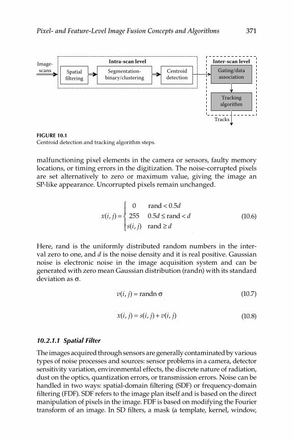
Pixel- and Feature-Level Image Fusion Concepts and Algorithms 371

malfunctioning pixel elements in the camera or sensors, faulty memory locations, or timing errors in the digitization. The noise-corrupted pixels are set alternatively to zero or maximum value, giving the image an SP-like appearance. Uncorrupted pixels remain unchanged.

x(i, j) =0 rand < 0.5d

255 0.5d ≤ rand < d

s(i, j) rand ≥ d

⎧

⎨⎪

⎩⎪

(10.6)

Here, rand is the uniformly distributed random numbers in the inter-val zero to one, and d is the noise density and it is real positive. Gaussian noise is electronic noise in the image acquisition system and can be generated with zero mean Gaussian distribution (randn) with its standard deviation as σ.

v(i, j) = randn σ (10.7)

x(i, j) = s(i, j) + v(i, j) (10.8)

10.2.1.1 Spatial Filter

The images acquired through sensors are generally contaminated by various types of noise processes and sources: sensor problems in a camera, detector sensitivity variation, environmental effects, the discrete nature of radiation, dust on the optics, quantization errors, or transmission errors. Noise can be handled in two ways: spatial-domain fi ltering (SDF) or frequency-domain fi ltering (FDF). SDF refers to the image plan itself and is based on the direct manipulation of pixels in the image. FDF is based on modifying the Fourier transform of an image. In SD fi lters, a mask (a template, kernel, window,

FIGURE 10.1 Centroid detection and tracking algorithm steps.

Intra-scan level

Spatialfiltering

Segmentation- binary/clustering

Centroiddetection

Image-scans

Inter-scan levelGating/dataassociation

Trackingalgorithm

Tracks

372 Multi-Sensor Data Fusion: Theory and Practice

or fi lter) is a small 2D (of 3 × 3 dimension) array or image in which the coeffi cients determine the process, such as image smoothing or sharpening [4]. The two primary categories of spatial fi lters for noise removal from the image are mean fi lters (linear) and order (nonlinear) fi lters.

10.2.1.2 Linear Spatial Filters

Linear fi ltering is achieved by local convolution with size n × n kernel mask and by a series of shift-multiply-sum operators with the n × n kernel. In this process (with a smoothing kernel mask), the brightness value of each pixel is replaced by a weighted average of the pixel brightness values in a neighborhood surrounding the pixel. The weighting factors for various pixels in the neighborhood are determined by the corresponding values in the mask. If the brightness value of any neighborhood pixel is unusual due to the infl uence of noise, then the brightness averaging will tend to reduce the effect of the noise by distributing it among the neighboring pixels.

y(i, j) = x(k, l)h(i − k, j − l)

l= j−w

j+w

∑k=i−w

i+w

∑ (10.9)

Here, x is the input image, h is the fi lter function/impulse response/ convolution mask, y is the output image, (i, j) is the index of the image pixel, i, j = 1, 2, ..., N, w = (n − 1)/2, N is the size of the input image, and n × n is the order of the fi lter or mask (an odd number). The mean fi lter is the simplest linear spatial fi lter. The coeffi cients in the kernel are nonnega-tive and equal. Masks of different sizes can be obtained as

hk = ones(k, k)

k2 (10.10)

Here, ones(k, k) is a k × k matrix having all elements as unity.

10.2.1.3 Nonlinear Spatial Filters

Nonlinear fi lters are data dependent. Order fi lters (OF) are a kind of nonlin-ear fi lter. OFs are based on order statistics and are implemented by arrang-ing the neighborhood pixels in order from the smallest to largest gray-level values. The most useful OF is the median fi lter, which selects the middle pixel value from the order set. The operation is performed by applying a slid-ing window similar to a convolution operation in a linear SDF. The median is computed by sorting all the pixel values from the surrounding neighbor-hood into numerical order and then replacing the pixel being considered with the middle pixel value. The unimportant or nonrepresentative pixel in a neighborhood will not signifi cantly affect the median value.

Pixel- and Feature-Level Image Fusion Concepts and Algorithms 373

10.2.2 Metrics for Performance Evaluation

The main idea is to compute a single number that refl ects the quality of the smoothed, fi ltered, and fused image.

10.2.2.1 Mean Square Error

The mean square error (MSE) of the true and fi ltered images will be nearly zero when the corresponding true and fi ltered image pixels are truly alike. The fi ltering algorithm that gives the minimum MSE value is preferable here.

MSE = 1

N 2s(i, j) − y(i, j)⎡⎣ ⎤⎦

2

j=1

N

∑i=1

N

∑ (10.11)

Here, s is the true image, y is the fi ltered image, N is the size of the image, and (i, j) is the index of the pixel.

10.2.2.2 Root Mean Square Error

Root mean square error (RMSE) will increase when the corresponding fi ltered image pixels deviate from the true image pixels. The fi ltering algo-rithm that gives the minimum value is preferable here.

RMSE = 1

N 2s(i, j) − y(i, j)⎡⎣ ⎤⎦

2

j=1

N

∑i=1

N

∑ (10.12)

10.2.2.3 Mean Absolute Error

Here again, a minimum mean absolute error (MAE) is sought for a good match.

MAE = 1

N 2s(i, j) − y(i, j)

j=1

N

∑i=1

N

∑ (10.13)

10.2.2.4 Percentage Fit Error

The fi ltering algorithm that gives the minimum percentage fi t error (PFE) is preferable here.

PFE =

norm(s − y)

norm(s)× 100 (10.14)

374 Multi-Sensor Data Fusion: Theory and Practice

10.2.2.5 Signal-to-Noise Ratio

The impact of noise on the image can be described by the signal-to-noise ratio (SNR). A comparison between two values for differently fi ltered images gives a comparison of the quality. The SNR will be infi nity when both true and fi ltered images are truly alike. The fi ltered algorithm that gives the high SNR value is preferable here.

SNR = 10 log10

s(i, j)2

j=1

N

∑i=1

N

∑

s(i, j) − y(i, j)⎡⎣ ⎤⎦2

j=1

N

∑i=1

N

∑

⎡

⎣

⎢⎢⎢⎢⎢

⎤

⎦

⎥⎥⎥⎥⎥

(10.15)

10.2.2.6 Peak Signal-to-Noise Ratio

The peak signal-to-noise ratio (PSNR) value will be infi nity when both true and fi ltered images are alike. The fi ltered algorithm that gives the high PSNR value is preferable here.

PSNRaf

= 10 log10

Imax2

[s(i, j) − y(i, j)]2

j=1

N

∑i=1

N

∑

⎡

⎣

⎢⎢⎢⎢⎢

⎤

⎦

⎥⎥⎥⎥⎥

(10.16)

Here, Imaxis the maximum pixel intensity value.

The performance of the mean and median fi lter to remove the SP noise with density 0.03 and Gaussian noise with mean zero and standard devia-tion σ = 1.4 is shown for simulated data in Figure 10.2. The performance of both types of fi lters to remove the salt-and-pepper (SAP) noise and Gaussian noise is found to be satisfactory.

10.2.3 Segmentation and Centroid Detection Techniques

T his section deals with image segmentation and CDT aspects.

10.2.3.1 Segmentation

Segmentation decomposes the image into two different regions: texture segmentation and particle segmentation. In texture segmentation, an image is partitioned into different regions (microimages) and each region is defi ned by a set of feature characteristics. In particle segmentation, an image is partitioned into object regions and background regions. Here, segmentation refers to the task of extracting objects or particles of interest

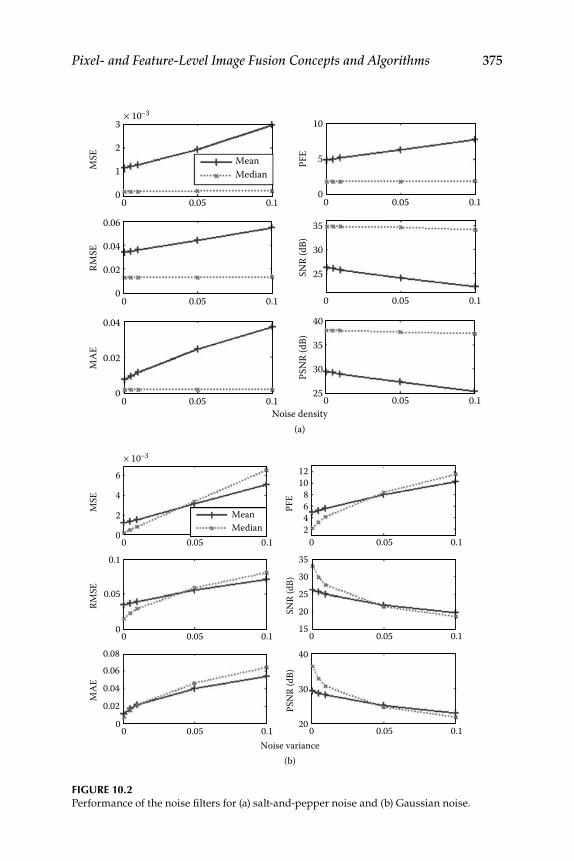
Pixel- and Feature-Level Image Fusion Concepts and Algorithms 375

FIGURE 10.2 Performance of the noise fi lters for (a) salt-and-pepper noise and (b) Gaussian noise.

10

5PFE

00 0.05 0.1

35

30

25SNR

(dB)

Noise density

0 0.05 0.1

× 10−33

2

1MSE

00 0.05 0.1

0.06

0.04

0.02RMSE

00 0.05 0.1

0.04

0.02

MAE

00 0.05 0.1

40

35

30

PSN

R (d

B)

250 0.05 0.1

(a)

MeanMedian

× 10−3

6

4

268

1012

42

253035

2015

0

MSE

RMSE

00 0.05 0.1

PFE

0.1

0.05

SNR

(dB)

Noise variance

0.05 0.1

000 0.05 0.1 0.05 0.1

MAE

0.080.060.040.02 PS

NR

(dB)

40

30

20000 0.05 0.1 0.05 0.1

(b)

MeanMedian

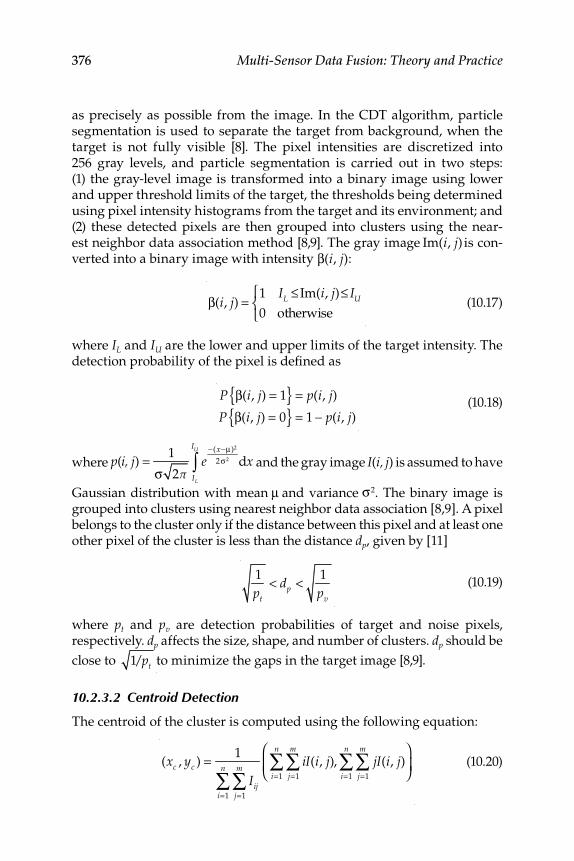
376 Multi-Sensor Data Fusion: Theory and Practice

as precisely as possible from the image. In the CDT algorithm, particle segmentation is used to separate the target from background, when the target is not fully visible [8]. The pixel intensities are discretized into 256 gray levels, and particle segmentation is carried out in two steps: (1) the gray-level image is transformed into a binary image using lower and upper threshold limits of the target, the thresholds being determined using pixel intensity histograms from the target and its environment; and (2) these detected pixels are then grouped into clusters using the near-est neighbor data association method [8,9]. The gray image Im(i, j) is con-verted into a binary image with intensity β(i, j):

β(i, j) =

1 IL ≤ Im(i, j)≤ IU

0 otherwise

⎧⎨⎩

(10.17)

where IL and IU are the lower and upper limits of the target intensity. The detection probability of the pixel is defi ned as

P β(i, j) = 1{ } = p(i, j)

P β(i, j) = 0{ } = 1 − p(i, j) (10.18)

where p(i, j) = 1

σ 2πe

−(x−μ)2

2σ2 dxIL

IU

∫ and the gray image I(i, j) is assumed to have

Gaussian distribution with mean μ and variance σ2. The binary image is grouped into clusters using nearest neighbor data association [8,9]. A pixel belongs to the cluster only if the distance between this pixel and at least one other pixel of the cluster is less than the distance dp, given by [11]

1

pt

< dp < 1

pv

(10.19)

where pt and pv are detection probabilities of target and noise pixels, respectively. dp affects the size, shape, and number of clusters. dp should be

close to

1/pt to minimize the gaps in the target image [8,9].

10.2.3.2 Centroid Detection

The centroid of the cluster is computed using the following equation:

(xc , yc ) = 1

Iijj=1

m

∑i=1

n

∑i

j=1

m

∑i=1

n

∑ I(i, j), jj=1

m

∑i=1

n

∑ I(i, j)⎛

⎝⎜⎞

⎠⎟ (10.20)

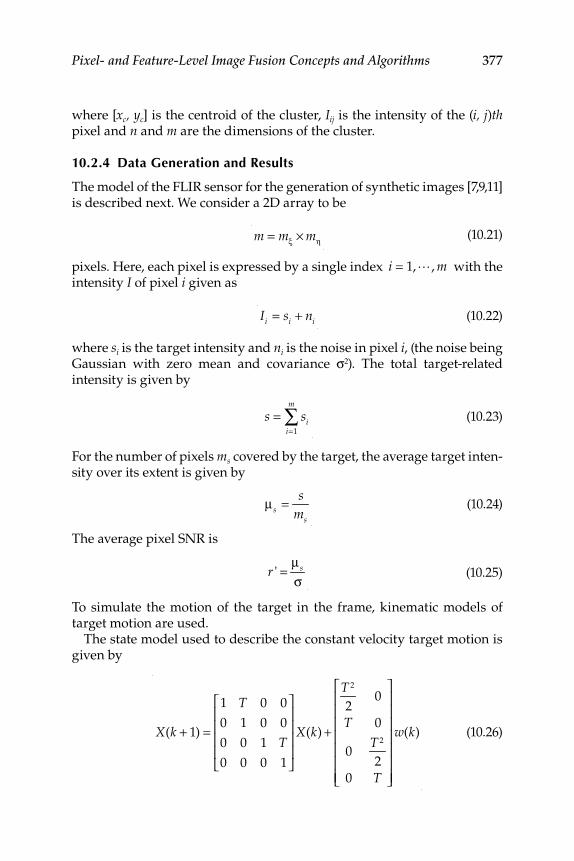
Pixel- and Feature-Level Image Fusion Concepts and Algorithms 377

where [xc, yc] is the centroid of the cluster, Iij is the intensity of the (i, j)th pixel and n and m are the dimensions of the cluster.

10.2.4 Data Generation and Results

The model of the FLIR sensor for the generation of synthetic images [7,9,11] is described next. We consider a 2D array to be

m = mξ × mη

(10.21)

pixels. Here, each pixel is expressed by a single index i = 1,L, m with the intensity I of pixel i given as

Ii = si + ni (10.22)

where si is the target intensity and ni is the noise in pixel i, (the noise being Gaussian with zero mean and covariance σ2). The total target- related intensity is given by

s = si

i=1

m

∑ (10.23)

For the number of pixels ms covered by the target, the average target inten-sity over its extent is given by

μs = s

ms

(10.24)

The average pixel SNR is

r ' =

μs

σ (10.25)

To simulate the motion of the target in the frame, kinematic models of target motion are used.

The state model used to describe the constant velocity target motion is given by

X(k + 1) =

1 T 0 0

0 1 0 0

0 0 1 T

0 0 0 1

⎡

⎣

⎢⎢⎢⎢

⎤

⎦

⎥⎥⎥⎥

X(k) +

T 2

20

T 0

0T 2

2

0 T

⎡

⎣

⎢⎢⎢⎢⎢⎢⎢

⎤

⎦

⎥⎥⎥⎥⎥⎥⎥

w(k) (10.26)

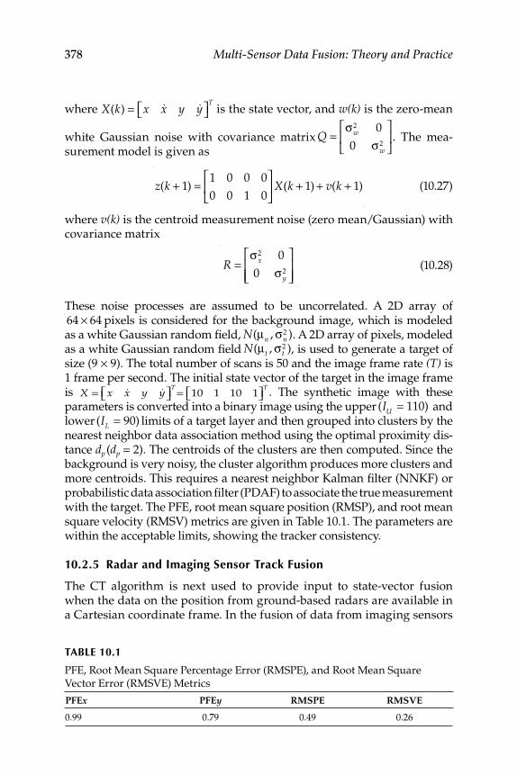
378 Multi-Sensor Data Fusion: Theory and Practice

where X(k) = x &x y &y⎡⎣ ⎤⎦T

is the state vector, and w(k) is the zero-mean

white Gaussian noise with covariance matrix Q =σw

2 0

0 σw2

⎡

⎣⎢

⎤

⎦⎥ . The mea-

surement model is given as

z(k + 1) =

1 0 0 0

0 0 1 0

⎡

⎣⎢

⎤

⎦⎥ X(k + 1) + v(k + 1) (10.27)

where v(k) is the centroid measurement noise (zero mean/Gaussian) with covariance matrix

R =σx

2 0

0 σy2

⎡

⎣⎢⎢

⎤

⎦⎥⎥

(10.28)

These noise processes are assumed to be uncorrelated. A 2D array of

64 × 64 pixels is considered for the background image, which is modeled as a white Gaussian random fi eld, N(μn , σn

2 ). A 2D array of pixels, modeled as a white Gaussian random fi eld N(μt , σt

2 ), is used to generate a target of size (9 × 9). The total number of scans is 50 and the image frame rate (T) is 1 frame per second. The initial state vector of the target in the image frame is X = x &x y &y⎡⎣ ⎤⎦

T= 10 1 10 1⎡⎣ ⎤⎦

T. The synthetic image with these

parameters is converted into a binary image using the upper (IU = 110) and lower (IL = 90) limits of a target layer and then grouped into clusters by the nearest neighbor data association method using the optimal proximity dis-tance dp (dp = 2). The centroids of the clusters are then computed. Since the background is very noisy, the cluster algorithm produces more clusters and more centroids. This requires a nearest neighbor Kalman fi lter (NNKF) or probabilistic data association fi lter (PDAF) to associate the true measurement with the target. The PFE, root mean square position (RMSP), and root mean square velocity (RMSV) metrics are given in Table 10.1. The parameters are within the acceptable limits, showing the tracker consistency.

10.2.5 Radar and Imaging Sensor Track Fusion

The CT algorithm is next used to provide input to state-vector fusion when the data on the position from ground-based radars are available in a Cartesian coordinate frame. In the fusion of data from imaging sensors

TABLE 10.1

PFE, Root Mean Square Percentage Error (RMSPE), and Root Mean Square Vector Error (RMSVE) Metrics

PFEx PFEy RMSPE RMSVE

0.99 0.79 0.49 0.26

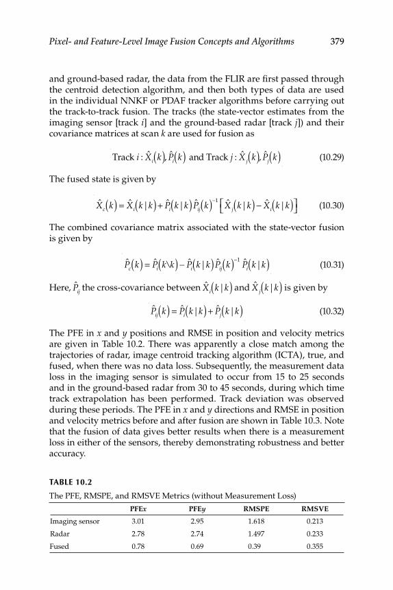
Pixel- and Feature-Level Image Fusion Concepts and Algorithms 379

and ground-based radar, the data from the FLIR are fi rst passed through the centroid detection algorithm, and then both types of data are used in the individual NNKF or PDAF tracker algorithms before carrying out the track-to-track fusion. The tracks (the state-vector estimates from the imaging sensor [track i ] and the ground-based radar [track j ]) and their covariance matrices at scan k are used for fusion as

Track i : Xi k( ), Pi k( ) and Track j : X j k( ), Pj k( ) (10.29)

The fused state is given by

Xc k( ) = Xi k|k( ) + Pi k|k( ) Pij k( )−1

X j k|k( ) − Xi k|k( )⎡⎣ ⎤⎦ (10.30)

The combined covariance matrix associated with the state-vector fusion is given by

Pc k( ) = Pi k\k( ) − Pi k|k( ) Pij k( )−1

Pi k|k( ) (10.31)

Here, Pij the cross-covariance between Xi k|k( ) and X j k|k( ) is given by

Pij k( ) = Pi k|k( ) + Pj k|k( ) (10.32)

The PFE in x and y positions and RMSE in position and velocity metrics are given in Table 10.2. There was apparently a close match among the trajectories of radar, image centroid tracking algorithm (ICTA), true, and fused, when there was no data loss. Subsequently, the measurement data loss in the imaging sensor is simulated to occur from 15 to 25 seconds and in the ground-based radar from 30 to 45 seconds, during which time track extrapolation has been performed. Track deviation was observed during these periods. The PFE in x and y directions and RMSE in position and velocity metrics before and after fusion are shown in Table 10.3. Note that the fusion of data gives better results when there is a measurement loss in either of the sensors, thereby demonstrating robustness and better accuracy.

TABLE 10.2

The PFE, RMSPE, and RMSVE Metrics (without Measurement Loss)

PFEx PFEy RMSPE RMSVE

Imaging sensor 3.01 2.95 1.618 0.213

Radar 2.78 2.74 1.497 0.233

Fused 0.78 0.69 0.39 0.355

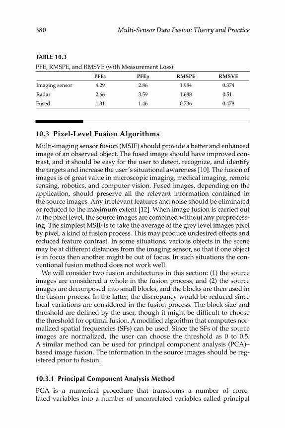
380 Multi-Sensor Data Fusion: Theory and Practice

10.3 Pixel-Level Fusion Algorithms

Multi-imaging sensor fusion (MSIF) should provide a better and enhanced image of an observed object. The fused image should have improved con-trast, and it should be easy for the user to detect, recognize, and identify the targets and increase the user’s situational awareness [10]. The fusion of images is of great value in microscopic imaging, medical imaging, remote sensing, robotics, and computer vision. Fused images, depending on the application, should preserve all the relevant information contained in the source images. Any irrelevant features and noise should be eliminated or reduced to the maximum extent [12]. When image fusion is carried out at the pixel level, the source images are combined without any preprocess-ing. The simplest MSIF is to take the average of the grey level images pixel by pixel, a kind of fusion process. This may produce undesired effects and reduced feature contrast. In some situations, various objects in the scene may be at different distances from the imaging sensor, so that if one object is in focus then another might be out of focus. In such situations the con-ventional fusion method does not work well.

We will consider two fusion architectures in this section: (1) the source images are considered a whole in the fusion process, and (2) the source images are decomposed into small blocks, and the blocks are then used in the fusion process. In the latter, the discrepancy would be reduced since local variations are considered in the fusion process. The block size and threshold are defi ned by the user, though it might be diffi cult to choose the threshold for optimal fusion. A modifi ed algorithm that computes nor-malized spatial frequencies (SFs) can be used. Since the SFs of the source images are normalized, the user can choose the threshold as 0 to 0.5. A similar method can be used for principal component analysis (PCA)–based image fusion. The information in the source images should be reg-istered prior to fusion.

10.3.1 Principal Component Analysis Method

PCA is a numerical procedure that transforms a number of corre-lated variables into a number of uncorrelated variables called principal

TABLE 10.3

PFE, RMSPE, and RMSVE (with Measurement Loss)

PFEx PFEy RMSPE RMSVE

Imaging sensor 4.29 2.86 1.984 0.374

Radar 2.66 3.59 1.688 0.51

Fused 1.31 1.46 0.736 0.478

Pixel- and Feature-Level Image Fusion Concepts and Algorithms 381

components (PCs; see the Appendix) [9]: (1) the fi rst PC accounts for much of the variance in the data, and each succeeding component accounts for much of the remaining variance; the fi rst PC is along the direction with the maximum variance; (2) the second component is constrained to lie in the subspace perpendicular to the fi rst component; within the subspace this component points to the direction of maximum variance; and (3) the third component is taken in the maximum variance direction in the subspace perpendicular to the fi rst two, and so on. PC basis vectors depend on the data set. Let X be a d -dimensional random vector with zero mean, and orthonormal projection matrix V be such that Y = VT X . The covariance ofY, cov(Y) is a diagonal matrix. Using simple matrix algebra we get [9]

cov(Y) = E YYT{ }= E VT X( ) VT X( )T{ }= E VT X( ) XTV( ){ }= VTE XXT{ }V

= VT cov(X)V

(10.33)

Multiplying both sides of Equation 10.33 by V, we get

V cov(Y) = VVT cov(X)V

= cov(X)V

(10.34)

We can write V as V = [V1,V

2, ...,Vd ] and cov(Y) in the diagonal form as

λ1

0 L 0 0

0 λ2

L 0 0

M M O M M0 0 L λd−1

0

0 0 L 0 λd

⎡

⎣

⎢⎢⎢⎢⎢⎢

⎤

⎦

⎥⎥⎥⎥⎥⎥

(10.35)

By substituting Equation 10.35 in Equation 10.34, we get

λ1V

1, λ

2V

2, ..., λdVd⎡⎣ ⎤⎦ = cov(X)V

1, cov(X)V

2, ..., cov(X)Vd⎡⎣ ⎤⎦ (10.36)

This is rewritten as

λ iVi = cov(X)Vi (10.37)

where i = 1, 2, ..., d and Vi is an eigenvector of cov(X).

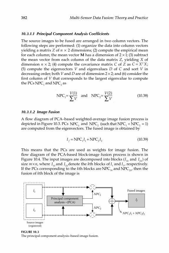
382 Multi-Sensor Data Fusion: Theory and Practice

10.3.1.1 Principal Component Analysis Coeffi cients

The source images to be fused are arranged in two column vectors. The following steps are performed: (1) organize the data into column vectors yielding a matrix Z of n × 2 dimensions; (2) compute the empirical mean for each column; the mean vector M has a dimension of 2 × l; (3) subtract the mean vector from each column of the data matrix Z, yielding X of dimension n × 2; (4) compute the covariance matrix C of Z as C = XT X; (5) compute the eigenvectors V and eigenvalues D of C and sort V in decreasing order; both V and D are of dimension 2 × 2; and (6) consider the fi rst column of V that corresponds to the largest eigenvalue to compute the PCs NPC

1and NPC

2as

NPC

1= V(1)

V∑and NPC

2= V(2)

V∑ (10.38)

10.3.1.2 Image Fusion

A fl ow diagram of PCA–based weighted-average image fusion process is depicted in Figure 10.3. PCs NPC

1 and NPC

2 (such that NPC

1+ NPC

2= 1)

are computed from the eigenvectors. The fused image is obtained by

I f = NPC

1I

1+ NPC

2I

2 (10.39)

This means that the PCs are used as weights for image fusion. The fl ow diagram of the PCA-based block-image fusion process is shown in Figure 10.4. The input images are decomposed into blocks (I1k and I

2k) of size m × n , where I

1k and I2kdenote the k th blocks of I

1and I

2, respectively.

If the PCs corresponding to the k th blocks are NPC1k and NPC

2k, then the fusion of k th block of the image is

FIGURE 10.3 The p rincipal component analysis–based image fusion.

Source images(registered)

Principal componentanalysis −(PCA)

Fused images NPC1

NPC2

NPC1I1 + NPC2I2

I1

I2

If

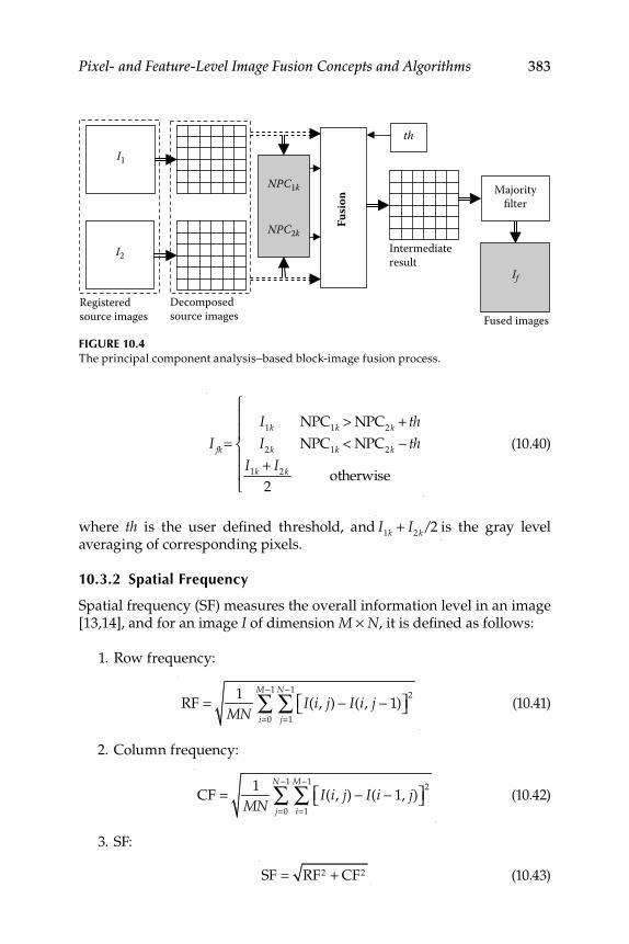
Pixel- and Feature-Level Image Fusion Concepts and Algorithms 383

I fk =I

1k NPC1k > NPC

2k + th

I2k NPC

1k < NPC2k − th

I1k + I

2k

2otherwise

⎧

⎨

⎪⎪

⎩

⎪⎪

(10.40)

where th is the user defi ned threshold, and I

1k + I2k/2 is the gray level

averaging of corresponding pixels.

10.3.2 Spatial Frequency

Spatial frequency (SF) measures the overall information level in an image [13,14], and for an image I of dimension M × N , it is defi ned as follows:

1. Row frequency:

RF = 1

MNI(i, j) − I(i, j − 1)⎡⎣ ⎤⎦

2

j=1

N −1

∑i=0

M−1

∑ (10.41)

2. Column frequency:

CF = 1

MNI(i, j) − I(i − 1, j)⎡⎣ ⎤⎦

2

i=1

M−1

∑j=0

N −1

∑ (10.42)

3. SF:

SF = RF2 + CF2 (10.43)

FIGURE 10.4 The principal component analysis–based block-image fusion process.

Fused images

NPC1k

NPC2k

Fusi

on Majority

filter

Registeredsource images

Decomposedsource images

Intermediateresult

thI1

If

I2

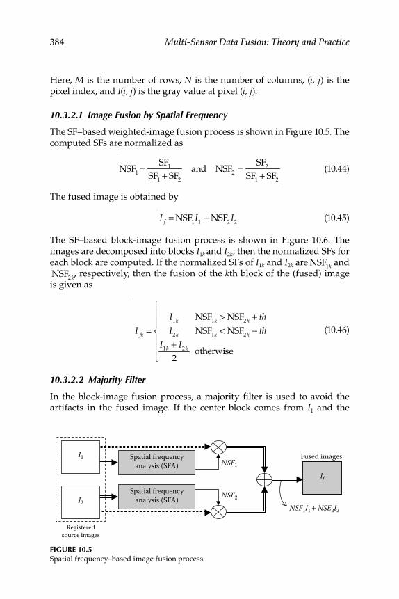
384 Multi-Sensor Data Fusion: Theory and Practice

Here, M is the number of rows, N is the number of columns, (i, j) is the pixel index, and I(i, j) is the gray value at pixel (i, j).

10.3.2.1 Image Fusion by Spatial Frequency

The SF–based weighted-image fusion process is shown in Figure 10.5. The computed SFs are normalized as

NSF1

=SF

1

SF1

+ SF2

and NSF2

=SF

2

SF1

+ SF2

(10.44)

The fused image is obtained by

I f = NSF

1I

1+ NSF

2I

2 (10.45)

The SF–based block-image fusion process is shown in Figure 10.6. The images are decomposed into blocks I1k and I2k; then the normalized SFs for each block are computed. If the normalized SFs of I1k and I2k are NSF

1k and

NSF2k, respectively, then the fusion of the k th block of the (fused) image

is given as

I fk =I

1k NSF1k > NSF

2k + th

I2k NSF

1k < NSF2k − th

I1k + I

2k

2otherwise

⎧

⎨

⎪⎪

⎩

⎪⎪

(10.46)

10.3.2.2 Majority Filter

In the block-image fusion process, a majority fi lter is used to avoid the artifacts in the fused image. If the center block comes from I1 and the

FIGURE 10.5 Spatial frequency–based image fusion process.

Registeredsource images

Fused images NSF1

NSF2

NSF1I1 + NSE2I2

I1

I2

If

Spatial frequencyanalysis (SFA)

Spatial frequencyanalysis (SFA)

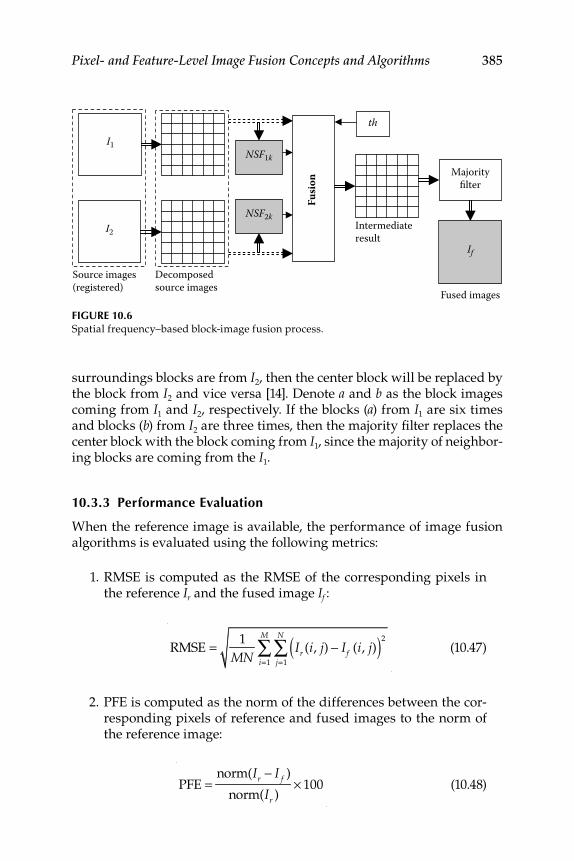
Pixel- and Feature-Level Image Fusion Concepts and Algorithms 385

surroundings blocks are from I2, then the center block will be replaced by the block from I2 and vice versa [14]. Denote a and b as the block images coming from I1 and I2, respectively. If the blocks (a) from I1 are six times and blocks (b) from I2 are three times, then the majority fi lter replaces the center block with the block coming from I1, since the majority of neighbor-ing blocks are coming from the I1.

10.3.3 Performance Evaluation

When the reference image is available, the performance of image fusion algorithms is evaluated using the following metrics:

1. RMSE is computed as the RMSE of the corresponding pixels in the reference Ir and the fused image If :

RMSE = 1

MNIr (i, j) − If (i, j)( )2

j=1

N

∑i=1

M

∑ (10.47)

2. PFE is computed as the norm of the differences between the cor-responding pixels of reference and fused images to the norm of the reference image:

PFE =

norm(Ir − I f )

norm(Ir )× 100 (10.48)

FIGURE 10.6 Spatial frequency–based block-image fusion process.

Fused images

NSF1k

NSF2k

Fusi

on Majority

filter

Source images(registered)

Decomposedsource images

Intermediateresult

thI1

If

I2

386 Multi-Sensor Data Fusion: Theory and Practice

3. MAE is computed as the MAE of the corresponding pixels in reference and fused images:

MAE = 1

MNIr(i, j) − If (i, j)

j=1

N

∑i=1

M

∑ (10.49)

4. SNR is computed as

SNR = 20log10

(Ir(i, j))2

j=1

N

∑i=1

M

∑

(Ir(i, j) − If (i, j))2

j=1

N

∑i=1

M

∑

⎛

⎝

⎜⎜⎜⎜

⎞

⎠

⎟⎟⎟⎟

(10.50)

5. PSNR is computed as

PSNR = 20log10

L2

1

MNIr(i, j) − If (i, j)( )2

j=1

N

∑i=1

M

∑

⎛

⎝

⎜⎜⎜⎜

⎞

⎠

⎟⎟⎟⎟

(10.51)

Here, L is the number of gray levels in the image.

6. Correlation shows the correlation between the reference and fused images:

CORR =2Crf

Cr + C f

(10.52)

Here,

Cr = Ir(i, j)2

j=1

N

∑i=1

M

∑ , C f = I f (i, j)2

j=1

N

∑i=1

M

∑ , and

Crf = Ir(i, j)I f (i, j)j=1

N

∑i=1

M

∑

7. MI [16] is given as

MI = hIrI f(i, j)log

2

hIrI f(i, j)

hIr(i, j)hI f

(i, j)

⎛

⎝⎜⎜

⎞

⎠⎟⎟j=1

N

∑i=1

M

∑ (10.53)

8. The universal quality index [16] measures how much of the salient information contained in the reference image has been transformed into the fused image. The metric range is −1 to 1 and the best value 1

Pixel- and Feature-Level Image Fusion Concepts and Algorithms 387

would be achieved if and only if the reference and fused images are alike. The lowest value of −1 would occur when I f = 2μ Ir

− Ir :

QI =4σ Ir I f

μ Ir+ μ I f( )

σ It

2 + σ I f

2( ) μ Ir

2 + μ I f

2( ) (10.54)

Here,

μ Ir= 1

MNIr(i, j),

j=1

N

∑i=1

M

∑ μ I f= 1

MNIf (i, j)

j=1

N

∑i=1

M

∑

σ Ir

2 = 1

MN − 1Ir(i, j) − μ Ir

( )2

j=1

N

∑i=1

M

∑ , σ I f

2 = 1

MN − 1If (i, j) − μ I f( )2

j=1

N

∑i=1

M

∑

σ Ir I f

2 = 1

MN − 1Ir(i, j) − μ Ir

( )j=1

N

∑i=1

M

∑ If (i, j) − μ I f( )

9. Measure of structural similarity compares local patterns of pixel intensities that are normalized for luminance and contrast. Nat-ural image signals are highly structured and their pixels reveal strong dependencies that carry information about the structure of the object. It is given as

SSIM =2μ Ir

μ I f+ C

1( ) 2σ Ir I f+ C

2( )μ Ir

2 + μ I f

2 + C1( ) σ Ir

2 + σ I f

2 + C2( ) (10.55)

Here, C1 is a constant that is included to avoid instability when

μ Ir

2 + μ I f

2 is close to zero and C2 is a constant that is included to

avoid instability when σ Ir

2 + σ I f

2 is close to zero.

10.3.3.1 Results and Discussion

The true image It is shown in Figure 10.7 and the source images to be fused, I1 and I2, are shown in Figure 10.8. The source images have been created by blurring a portion of the reference image with a Gaussian mask using a diameter of 12 pixels. The images fused by PCA and SF and the correspond-ing error images (with the procedure given for the fi rst method) are shown in Figure 10.9. The performance metrics are shown in Table 10.4. From these results, note that image fusion by SF is marginally better or similar to PCA.

Figure 10.10a gives a 100 × 100 image block and Figure 10.10b through d shows the degraded images after blurring with a disk of radius 5, 9, and 21 pixels, respectively. Figure 10.10a is one of the source images I1, and

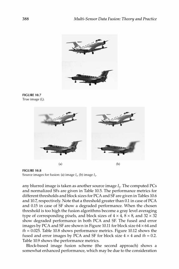
388 Multi-Sensor Data Fusion: Theory and Practice

any blurred image is taken as another source image I2. The computed PCs and normalized SFs are given in Table 10.5. The performance metrics for different thresholds and block sizes for PCA and SF are given in Tables 10.6 and 10.7, respectively. Note that a threshold greater than 0.1 in case of PCA and 0.15 in case of SF show a degraded performance. When the chosen threshold is too high the fusion algorithms become a gray level averaging type of corresponding pixels, and block sizes of 4 × 4, 8 × 8, and 32 × 32 show degraded performance in both PCA and SF. The fused and error images by PCA and SF are shown in Figure 10.11 for block size 64 × 64 and th = 0.025. Table 10.8 shows performance metrics. Figure 10.12 shows the fused and error images by PCA and SF for block size 4 × 4 and th = 0.2. Table 10.9 shows the performance metrics.

Block-based image fusion scheme (the second approach) shows a somewhat enhanced performance, which may be due to the consideration

FIGURE 10.7 True image (It).

FIGURE 10.8 Source images for fusion: (a) image I1, (b) image I2.

(a) (b)

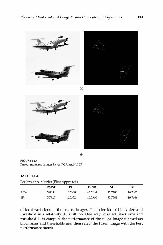
Pixel- and Feature-Level Image Fusion Concepts and Algorithms 389

of local variations in the source images. The selection of block size and threshold is a relatively diffi cult job. One way to select block size and threshold is to compute the performance of the fused image for various block sizes and thresholds and then select the fused image with the best performance metric.

TABLE 10.4

Performance Metrics (First Approach)

RMSE PFE PSNR SD SF

PCA 5.8056 2.5388 40.5264 55.7286 16.7602

SF 5.7927 2.5332 40.5360 55.7302 16.7636

FIGURE 10.9 Fused and error images by (a) PCA and (b) SF.

(a)

(b)

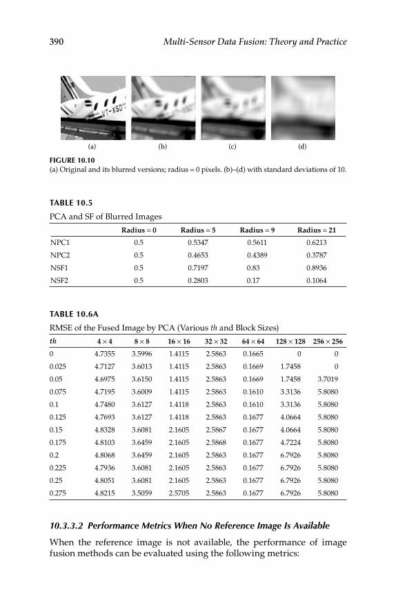
390 Multi-Sensor Data Fusion: Theory and Practice

10.3.3.2 Performance Metrics When No Reference Image Is Available

When the reference image is not available, the performance of image fusion methods can be evaluated using the following metrics:

TABLE 10.6A

RMSE of the Fused Image by PCA (Various th and Block Sizes)

th 4 × 4 8 × 8 16 × 16 32 × 32 64 × 64 128 × 128 256 × 256

0 4.7355 3.5996 1.4115 2.5863 0.1665 0 0

0.025 4.7127 3.6013 1.4115 2.5863 0.1669 1.7458 0

0.05 4.6975 3.6150 1.4115 2.5863 0.1669 1.7458 3.7019

0.075 4.7195 3.6009 1.4115 2.5863 0.1610 3.3136 5.8080

0.1 4.7480 3.6127 1.4118 2.5863 0.1610 3.3136 5.8080

0.125 4.7693 3.6127 1.4118 2.5863 0.1677 4.0664 5.8080

0.15 4.8328 3.6081 2.1605 2.5867 0.1677 4.0664 5.8080

0.175 4.8103 3.6459 2.1605 2.5868 0.1677 4.7224 5.8080

0.2 4.8068 3.6459 2.1605 2.5863 0.1677 6.7926 5.8080

0.225 4.7936 3.6081 2.1605 2.5863 0.1677 6.7926 5.8080

0.25 4.8051 3.6081 2.1605 2.5863 0.1677 6.7926 5.8080

0.275 4.8215 3.5059 2.5705 2.5863 0.1677 6.7926 5.8080

FIGURE 10.10 (a) Original and its blurred versions; radius = 0 pixels. (b)–(d) with standard deviations of 10.

(a) (b) (c) (d)

TABLE 10.5

PCA and SF of Blurred Images

Radius = 0 Radius = 5 Radius = 9 Radius = 21

NPC1 0.5 0.5347 0.5611 0.6213

NPC2 0.5 0.4653 0.4389 0.3787

NSF1 0.5 0.7197 0.83 0.8936

NSF2 0.5 0.2803 0.17 0.1064

Pixel- and Feature-Level Image Fusion Concepts and Algorithms 391

1. Standard deviation (STD) measures the contrast in the fused image. An image with high contrast would have a high standard deviation:

SD = (i − i )2 hI f

(i)i=0

L

∑ , i = ihI fi=0

L

∑ (10.56)

TABLE 10.6B

PSNR of the Fused Image by PCA (Various th and Block Sizes)

th 4 × 4 8 × 8 16 × 16 32 × 32 64 × 64 128 × 128 256 × 256

0 41.4111 42.6023 46.6680 44.0381 55.9513 Inf Inf

0.025 41.4321 42.6002 46.6680 44.0381 55.9395 45.7449 Inf

0.05 41.4461 42.5837 46.6680 44.0381 55.9395 45.7449 42.4806

0.075 41.4258 42.6007 46.6680 44.0381 56.0964 42.9617 40.5245

0.1 41.3997 42.5865 46.6672 44.0381 56.0964 42.9617 40.5245

0.125 41.3803 42.5865 46.6672 44.0381 55.9201 42.0727 40.5245

0.15 41.3228 42.5920 44.8192 44.0373 55.9201 42.0727 40.5245

0.175 41.3431 42.5468 44.8192 44.0372 55.9201 41.4232 40.5245

0.2 41.3462 42.5468 44.8192 44.0381 55.9201 39.8444 40.5245

0.225 41.3581 42.5920 44.8192 44.0381 55.9201 39.8444 40.5245

0.25 41.3478 42.5920 44.8192 44.0381 55.9201 39.8444 40.5245

0.275 41.3330 42.7168 44.0646 44.0381 55.9201 39.8444 40.5245

TABLE 10.7A

RMSE of the Fused Image by SF (Various th and Block Sizes)

th 4 × 4 8 × 8 16 × 16 32 × 32 64 × 64 128 × 128 256 × 256

0 3.9654 2.1281 1.4212 2.5942 0.1665 0 0

0.025 3.9016 1.8885 1.4212 2.5942 0.1610 0 0

0.05 3.9482 1.8885 1.4212 2.5942 0.1610 1.7458 0

0.075 3.9958 1.9016 1.4212 2.5942 0.1610 1.7458 0

0.1 4.0546 1.9226 1.4212 2.5942 0.1610 1.7458 0

0.125 4.0008 1.9226 1.4212 2.5942 0.1610 1.7458 0

0.15 4.0448 2.1034 1.4212 0.2027 0.1677 1.7458 0

0.175 3.9632 2.2860 1.4212 0.2027 0.1677 2.9331 3.7019

0.2 4.0151 2.2860 1.4212 0.2027 0.1677 2.9331 3.7019

0.225 3.9613 2.1687 1.4212 0.2027 0.1677 2.9331 5.8080

0.25 3.9624 2.2751 1.4212 0.2027 0.1677 2.9331 5.8080

0.275 3.7989 2.2751 1.4212 0.2027 0.1677 2.9331 5.8080

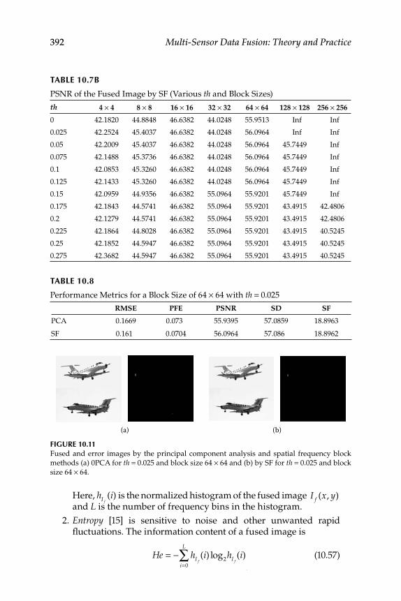
392 Multi-Sensor Data Fusion: Theory and Practice

Here, hI f(i) is the normalized histogram of the fused image I f (x, y)

and L is the number of frequency bins in the histogram.

2. Entropy [15] is sensitive to noise and other unwanted rapid fl uctuations. The information content of a fused image is

He = − hI f

(i) log2hI f

(i)i=0

L

∑ (10.57)

TABLE 10.8

Performance Metrics for a Block Size of 64 × 64 with th = 0.025

RMSE PFE PSNR SD SF

PCA 0.1669 0.073 55.9395 57.0859 18.8963

SF 0.161 0.0704 56.0964 57.086 18.8962

FIGURE 10.11 Fused and error images by the principal component analysis and spatial frequency block

methods (a) 0PCA for th = 0.025 and block size 64 × 64 and (b) by SF for th = 0.025 and block

size 64 × 64.

(a) (b)

TABLE 10.7B

PSNR of the Fused Image by SF (Various th and Block Sizes)

th 4 × 4 8 × 8 16 × 16 32 × 32 64 × 64 128 × 128 256 × 256

0 42.1820 44.8848 46.6382 44.0248 55.9513 Inf Inf

0.025 42.2524 45.4037 46.6382 44.0248 56.0964 Inf Inf

0.05 42.2009 45.4037 46.6382 44.0248 56.0964 45.7449 Inf

0.075 42.1488 45.3736 46.6382 44.0248 56.0964 45.7449 Inf

0.1 42.0853 45.3260 46.6382 44.0248 56.0964 45.7449 Inf

0.125 42.1433 45.3260 46.6382 44.0248 56.0964 45.7449 Inf

0.15 42.0959 44.9356 46.6382 55.0964 55.9201 45.7449 Inf

0.175 42.1843 44.5741 46.6382 55.0964 55.9201 43.4915 42.4806

0.2 42.1279 44.5741 46.6382 55.0964 55.9201 43.4915 42.4806

0.225 42.1864 44.8028 46.6382 55.0964 55.9201 43.4915 40.5245

0.25 42.1852 44.5947 46.6382 55.0964 55.9201 43.4915 40.5245

0.275 42.3682 44.5947 46.6382 55.0964 55.9201 43.4915 40.5245

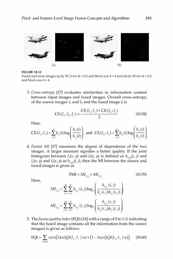
Pixel- and Feature-Level Image Fusion Concepts and Algorithms 393

3. Cross-entropy [17] evaluates similarities in information content between input images and fused images. Overall cross-entropy of the source images I1 and I2 and the fused image If is

CE(I

1, I

2; If ) =

CE(I1; If ) + CE(I

2; I f )

2 (10.58)

Here,

CE(I1; I f ) = hI1

(i) loghI1

(i)

hI f(i)

⎛

⎝⎜⎜

⎞

⎠⎟⎟i=0

L

∑ and CE(I2; I f ) = hI2

(i) loghI2

(i)

hI f(i)

⎛

⎝⎜⎜

⎞

⎠⎟⎟i=0

L

∑

4. Fusion MI [17] measures the degree of dependence of the two images. A larger measure signifi es a better quality. If the joint histogram between I1(x, y) and If (x, y) is defi ned as hI1If

(i, j) and I2(x, y) and If (x, y) as hI2If

(i, j), then the MI between the source and fused images is given as

FMI = MII1I f

+ MII2I f (10.59)

Here,

MII1I f= hI1I f

(i, j) log2

hI1I f(i, j)

hI1(i, j)hI f

(i, j)

⎛

⎝⎜⎜

⎞

⎠⎟⎟j=1

N

∑i=1

M

∑ ;

MII2I f= hI2I f

(i, j) log2

hI2I f(i, j)

hI2(i, j)hI f

(i, j)

⎛

⎝⎜⎜

⎞

⎠⎟⎟j=1

N

∑i=1

M

∑

5. The fusion quality index (FQI) [18] with a range of 0 to 1 (1 indicating that the fused image contains all the information from the source images) is given as follows:

FQI = c(w) λ(w)QI(I1, I f |w) + 1 − λ(w)( )QI(I

2, I f |w)( )

w∈W∑ (10.60)

FIGURE 10.12 Fused and error images (a) by PCA for th = 0.2 and block size 4 × 4 and (b) by SF for th = 0.2

and block size 4 × 4.

(a) (b)

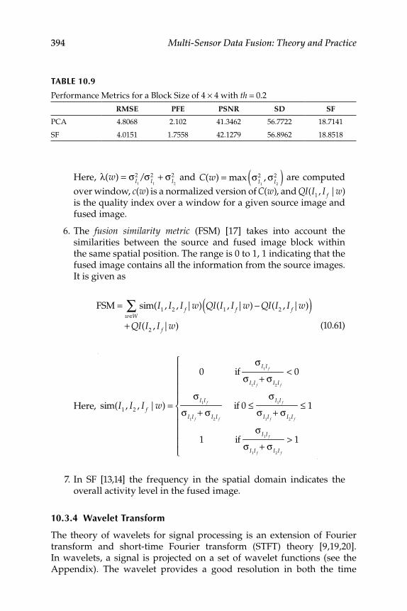
394 Multi-Sensor Data Fusion: Theory and Practice

Here, λ(w) = σ I1

2 /σ I1

2 + σ I2

2 and C(w) = max σ I1

2 , σ I2

2( ) are computed

over window, c(w) is a normalized version of C(w), and QI(I1, I f |w)

is the quality index over a window for a given source image and fused image.

6. The fusion similarity metric (FSM) [17] takes into account the similarities between the source and fused image block within the same spatial position. The range is 0 to 1, 1 indicating that the fused image contains all the information from the source images. It is given as

FSM = sim(I

1, I

2, I f|w) QI(I

1, I f|w) − QI(I

2, I f|w)( )

w∈W∑

+ QI(I

2, I f|w)

(10.61)

Here,

sim(I1, I

2, I f |w) =

0 ifσ I1I f

σ I1I f+ σ I2I f

< 0

σ I1I f

σ I1I f+ σ I2I f

if 0 ≤σ I1I f

σ I1I f+ σ I2I f

≤ 1

1 ifσ I1I f

σ I1I f+ σ I2I f

> 1

⎧

⎨

⎪⎪⎪⎪

⎩

⎪⎪⎪⎪

7. In SF [13,14] the frequency in the spatial domain indicates the overall activity level in the fused image.

10.3.4 Wavelet Transform

The theory of wavelets for signal processing is an extension of Fourier transform and short-time Fourier transform (STFT) theory [9,19,20]. In wavelets, a signal is projected on a set of wavelet functions (see the Appendix). The wavelet provides a good resolution in both the time

TABLE 10.9

Performance Metrics for a Block Size of 4 × 4 with th = 0.2

RMSE PFE PSNR SD SF

PCA 4.8068 2.102 41.3462 56.7722 18.7141

SF 4.0151 1.7558 42.1279 56.8962 18.8518

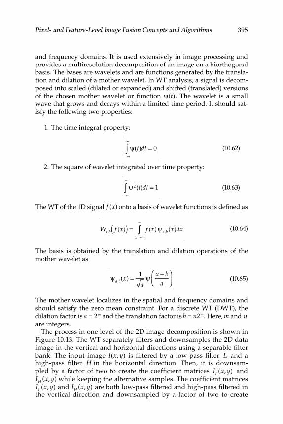
Pixel- and Feature-Level Image Fusion Concepts and Algorithms 395

and frequency domains. It is used extensively in image processing and provides a multiresolution decomposition of an image on a biorthogonal basis. The bases are wavelets and are functions generated by the transla-tion and dilation of a mother wavelet. In WT analysis, a signal is decom-posed into scaled (dilated or expanded) and shifted (translated) versions of the chosen mother wavelet or function ψ(t). The wavelet is a small wave that grows and decays within a limited time period. It should sat-isfy the following two properties:

1. The time integral property:

ψ(t)dt = 0

−∞

∞

∫ (10.62)

2. The square of wavelet integrated over time property:

ψ2 (t)dt = 1

−∞

∞

∫ (10.63)

The WT of the 1D signal f (x) onto a basis of wavelet functions is defi ned as

Wa ,b f (x)( ) = f (x)

x=−∞

∞

∫ ψ a ,b (x)dx (10.64)

The basis is obtained by the translation and dilation operations of the mother wavelet as

ψ a ,b(x) = 1

aψ x − b

a⎛⎝⎜

⎞⎠⎟

(10.65)

The mother wavelet localizes in the spatial and frequency domains and should satisfy the zero mean constraint. For a discrete WT (DWT), the dilation factor is a = 2m and the translation factor is b = n2m. Here, m and nare integers.

The process in one level of the 2D image decomposition is shown in Figure 10.13. The WT separately fi lters and downsamples the 2D data image in the vertical and horizontal directions using a separable fi lter bank. The input image I(x, y) is fi ltered by a low-pass fi lter L and a high-pass fi lter H in the horizontal direction. Then, it is downsam-pled by a factor of two to create the coeffi cient matrices IL (x, y) andIH (x, y) while keeping the alternative samples. The coeffi cient matricesIL (x, y) and IH (x, y) are both low-pass fi ltered and high-pass fi ltered in the vertical direction and downsampled by a factor of two to create

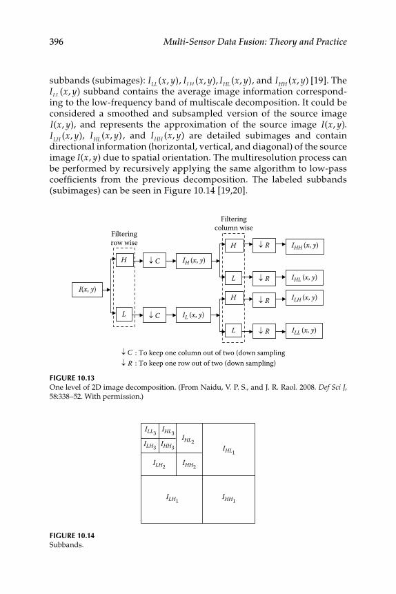
396 Multi-Sensor Data Fusion: Theory and Practice

subbands (subimages): ILL (x, y), ILH (x, y), IHL (x, y), and IHH (x, y) [19]. The ILL (x, y) subband contains the average image information correspond-ing to the low-frequency band of multiscale decomposition. It could be considered a smoothed and subsampled version of the source image I(x, y), and represents the approximation of the source image I(x, y).ILH (x, y), IHL (x, y) , and IHH (x, y) are detailed subimages and contain directional information (horizontal, vertical, and diagonal) of the source image I(x, y) due to spatial orientation. The multiresolution process can be performed by recursively applying the same algorithm to low-pass coeffi cients from the previous decomposition. The labeled subbands (subimages) can be seen in Figure 10.14 [19,20].

FIGURE 10.13 One level of 2D image decomposition. (From Naidu, V. P. S., and J. R. Raol. 2008. Def Sci J, 58:338–52. With permission.)

: To keep one column out of two (down sampling: To keep one row out of two (down sampling)

C R

H

L

R

C

R

H

H

L

L

C

ILL (x, y)

ILH (x, y)

IHL (x, y)

IHH (x, y)

IH (x, y)

IL (x, y)

I(x, y)

Filteringcolumn wise

Filteringrow wise

R

R

FIGURE 10.14 Subbands.

IHH1ILH1

ILH2

ILH3

ILL3

IHH3

IHL3

IHL1

IHL2

IHH2

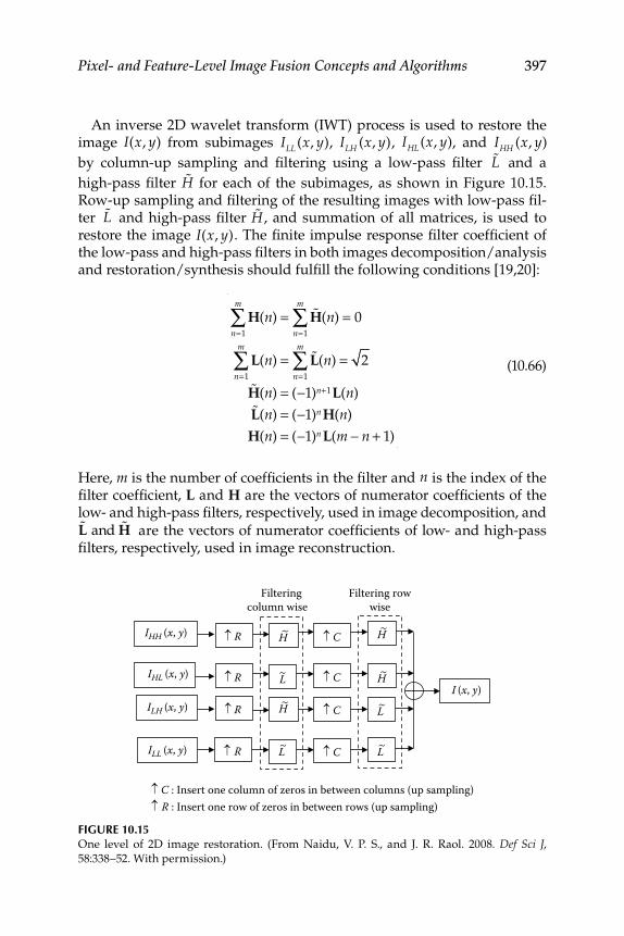
Pixel- and Feature-Level Image Fusion Concepts and Algorithms 397

An inverse 2D wavelet transform (IWT) process is used to restore the image I(x, y) from subimages ILL (x, y), ILH (x, y), IHL (x, y), and IHH (x, y)

by column-up sampling and fi ltering using a low-pass fi lter %L and a

high-pass fi lter %H for each of the subimages, as shown in Figure 10.15. Row-up sampling and fi ltering of the resulting images with low-pass fi l-ter %L and high-pass fi lter %H , and summation of all matrices, is used to restore the image I(x, y). The fi nite impulse response fi lter coeffi cient of the low-pass and high-pass fi lters in both images decomposition/analysis and restoration/synthesis should fulfi ll the following conditions [19,20]:

H(n)n=1

m

∑ = %H(n) = 0n=1

m

∑

L(n)n=1

m

∑ = %L(n) = 2n=1

m

∑%H(n) = (−1)n+1L(n)%L(n) = (−1)n H(n)

H(n) = (−1)n L(m − n + 1)

(10.66)

Here, m is the number of coeffi cients in the fi lter and n is the index of the fi lter coeffi cient, L and H are the vectors of numerator coeffi cients of the low- and high-pass fi lters, respectively, used in image decomposition, and %L and %H are the vectors of numerator coeffi cients of low- and high-pass fi lters, respectively, used in image reconstruction.

FIGURE 10.15 One level of 2D image restoration. (From Naidu, V. P. S., and J. R. Raol. 2008. Def Sci J, 58:338–52. With permission.)

R : Insert one row of zeros in between rows (up sampling) C : Insert one column of zeros in between columns (up sampling)

IHH (x, y)

IHL (x, y)I (x, y)

ILH (x, y)

ILL (x, y)

H~

L~

R H~

H~

L~

L~

C

Filteringcolumn wise

Filtering rowwise

L~

H~C

C

C

R

R

R

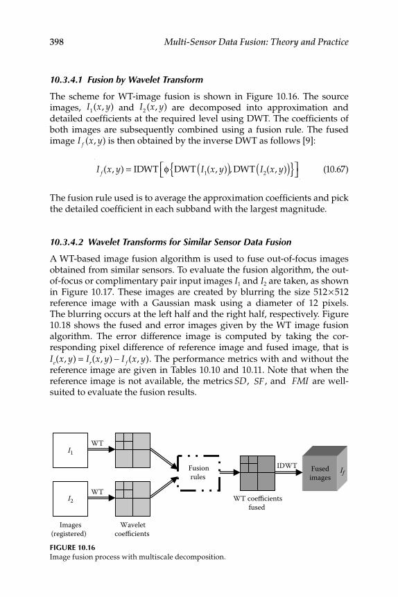
398 Multi-Sensor Data Fusion: Theory and Practice

10.3.4.1 Fusion by Wavelet Transform

The scheme for WT-image fusion is shown in Figure 10.16. The source images, I

1(x, y) and I

2(x, y) are decomposed into approximation and

detailed coeffi cients at the required level using DWT. The coeffi cients of both images are subsequently combined using a fusion rule. The fused image I f (x, y) is then obtained by the inverse DWT as follows [9]:

I f (x, y) = IDWT φ DWT I

1(x, y)( ), DWT I

2(x, y)( ){ }⎡

⎣⎤⎦ (10.67)

The fusion rule used is to average the approximation coeffi cients and pick the detailed coeffi cient in each subband with the largest magnitude.

10.3.4.2 Wavelet Transforms for Similar Sensor Data Fusion

A WT-based image fusion algorithm is used to fuse out-of-focus images obtained from similar sensors. To evaluate the fusion algorithm, the out-of-focus or complimentary pair input images I1 and I2 are taken, as shown in Figure 10.17. These images are created by blurring the size 512 × 512 reference image with a Gaussian mask using a diameter of 12 pixels. The blurring occurs at the left half and the right half, respectively. Figure 10.18 shows the fused and error images given by the WT image fusion algorithm. The error difference image is computed by taking the cor-responding pixel difference of reference image and fused image, that is

Ie(x, y) = Ir(x, y) − I f (x, y). The performance metrics with and without the reference image are given in Tables 10.10 and 10.11. Note that when the reference image is not available, the metrics SD, SF , and FMI are well-suited to evaluate the fusion results.

FIGURE 10.16 Image fusion process with multiscale decomposition.

Fusionrules

Images(registered)

Waveletcoefficients

WT coefficientsfused

I1

I2

IfFusedimages

WT

WT

IDWT

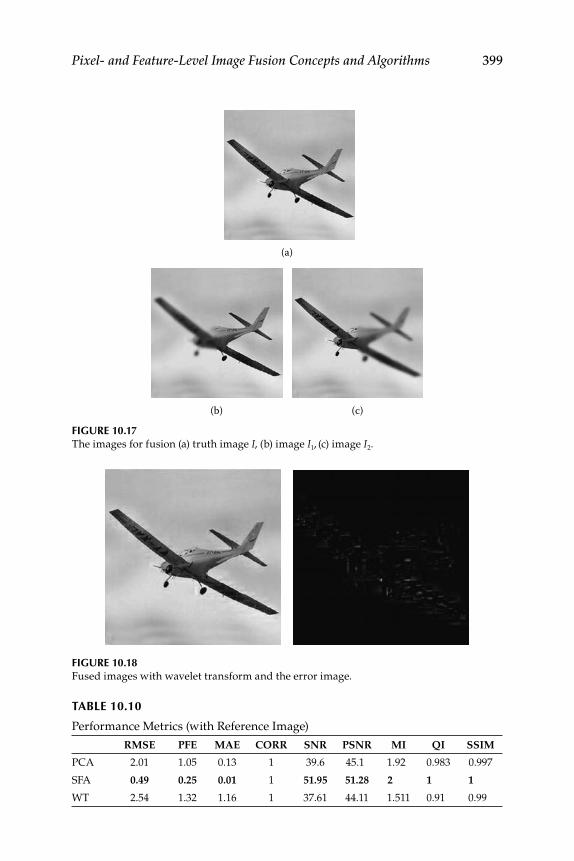
Pixel- and Feature-Level Image Fusion Concepts and Algorithms 399

TABLE 10.10

Performance Metrics (with Reference Image)

RMSE PFE MAE CORR SNR PSNR MI QI SSIM

PCA 2.01 1.05 0.13 1 39.6 45.1 1.92 0.983 0.997

SFA 0.49 0.25 0.01 1 51.95 51.28 2 1 1

WT 2.54 1.32 1.16 1 37.61 44.11 1.511 0.91 0.99

FIGURE 10.17 The images for fusion (a) truth image I, (b) image I1, (c) image I2.

(a)

(c)(b)

FIGURE 10.18 Fused images with wavelet transform and the error image.

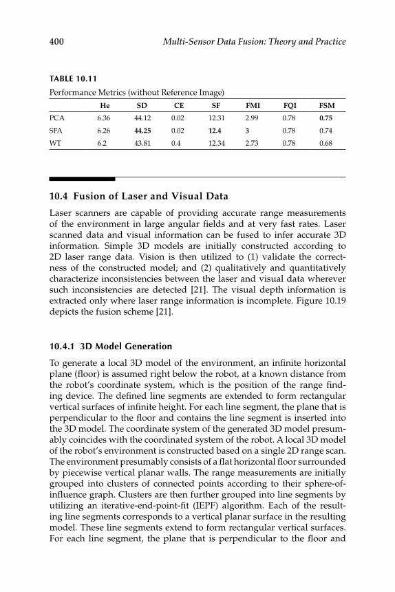
400 Multi-Sensor Data Fusion: Theory and Practice

10.4 Fusion of Laser and Visual Data

Laser scanners are capable of providing accurate range measurements of the environment in large angular fi elds and at very fast rates. Laser scanned data and visual information can be fused to infer accurate 3D information. Simple 3D models are initially constructed according to 2D laser range data. Vision is then utilized to (1) validate the correct-ness of the constructed model; and (2) qualitatively and quantitatively characterize inconsistencies between the laser and visual data wherever such inconsistencies are detected [21]. The visual depth information is extracted only where laser range information is incomplete. Figure 10.19 depicts the fusion scheme [21].

10.4.1 3D Model Generation

To generate a local 3D model of the environment, an infi nite horizontal plane (fl oor) is assumed right below the robot, at a known distance from the robot’s coordinate system, which is the position of the range fi nd-ing device. The defi ned line segments are extended to form rectangular vertical surfaces of infi nite height. For each line segment, the plane that is perpendicular to the fl oor and contains the line segment is inserted into the 3D model. The coordinate system of the generated 3D model presum-ably coincides with the coordinated system of the robot. A local 3D model of the robot’s environment is constructed based on a single 2D range scan. The environment presumably consists of a fl at horizontal fl oor surrounded by piecewise vertical planar walls. The range measurements are initially grouped into clusters of connected points according to their sphere-of-infl uence graph. Clusters are then further grouped into line segments by utilizing an iterative-end-point-fi t (IEPF) algorithm. Each of the result-ing line segments corresponds to a vertical planar surface in the resulting model. These line segments extend to form rectangular vertical surfaces. For each line segment, the plane that is perpendicular to the fl oor and

TABLE 10.11

Performance Metrics (without Reference Image)

He SD CE SF FMI FQI FSM

PCA 6.36 44.12 0.02 12.31 2.99 0.78 0.75

SFA 6.26 44.25 0.02 12.4 3 0.78 0.74

WT 6.2 43.81 0.4 12.34 2.73 0.78 0.68

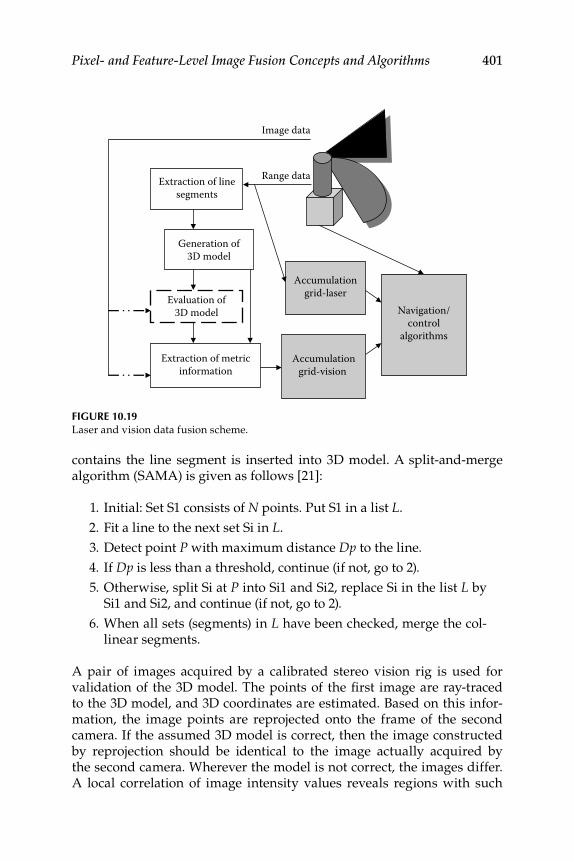
Pixel- and Feature-Level Image Fusion Concepts and Algorithms 401

contains the line segment is inserted into 3D model. A split-and-merge algorithm (SAMA) is given as follows [21]:

1. Initial: Set S1 consists of N points. Put S1 in a list L .

2. Fit a line to the next set Si in L .

3. Detect point P with maximum distance Dp to the line.

4. If Dp is less than a threshold, continue (if not, go to 2).

5. Otherwise, split Si at P into Si1 and Si2, replace Si in the list L by Si1 and Si2, and continue (if not, go to 2).

6. When all sets (segments) in L have been checked, merge the col-linear segments.

A pair of images acquired by a calibrated stereo vision rig is used for validation of the 3D model. The points of the fi rst image are ray-traced to the 3D model, and 3D coordinates are estimated. Based on this infor-mation, the image points are reprojected onto the frame of the second camera. If the assumed 3D model is correct, then the image constructed by reprojection should be identical to the image actually acquired by the second camera. Wherever the model is not correct, the images differ. A local correlation of image intensity values reveals regions with such

FIGURE 10.19 Laser and vision data fusion scheme.

Extraction of linesegments

Generation of3D model

Evaluation of3D model

Extraction of metricinformation

Accumulationgrid-laser

Accumulationgrid-vision

Navigation/control

algorithms

Image data

Range data

402 Multi-Sensor Data Fusion: Theory and Practice

inconsistencies. Vision is then further utilized to provide additional depth information in regions where the 2D range data proved to be insuffi cient.

10.4.2 Model Evaluation

Model evaluation procedure is described next [21]. Let M be the 3D model built according to range data acquired at time t 1, and let the I1 be an image acquired by a camera C1 at the same time, t 1. For each image point P1 = ( x 1, y 1) of I1, the coordinates ( x , y , and z ) of the corresponding 3D point P can be computed by ray-tracing it to the model M . If the assump-tions made for constructing the 3D model are correct, the coordinates ( x , y , and z ) found by the above procedure correspond to a real-world point on M . Let I2 be a second image acquired by the second camera of the stereoscopic system. Since the coordinate system of C2 with respect to the coordinate system of M is also known, the projection P2 = ( x 2, y 2) of P = ( x , y , and z ) on C2 can also be computed. Ray-tracing the points of I1 to fi nd 3D world coordinates and then back-projecting them to I2 leads to an analytical computation of point correspondences between I1 and I2.

If the assumptions made to form model M are correct, corresponding image points would actually be projections of the same world points and thus would share the same attributes, such as color, intensity, values, and intensity gradients. If the image points have different attributes, then there is a strong indication that the model is locally invalid. The normalized cross-correlation metric can be used to evaluate the correctness of the calculated point correspondences. Low values indicate the regions within the images that depict parts of the environment that do not conform to the 3D model.

10.5 Feature-Level Fusion Methods

2D and 3D intensity and color images have been extensively researched for object recognition problems [22]. A 3D representation provides addi-tional information. A 3D picture lacks texture information. A 2D image can complement 3D information. 2D images are localized in many details, such as eyebrows, eyes, nose, mouth, and facial hair, whereas 3D images are diffi cult to localize and are not accurate for such details. A robust sys-tem may require the fusion of 2D and 3D images. Then, nonclarity in one aspect, such as lighting problem, may be compensated by other aspects, such as depth features. Image fusion can be performed at the feature level, matching score level, or decision level, utilizing different fusion models, for example, sum, product, maximum, minimum, and major voting to combine the individual scores (normalized to range [0,l]). A multivariate

Pixel- and Feature-Level Image Fusion Concepts and Algorithms 403

polynomial (MP) technique provides an effective way to describe complex nonlinear input/output (I/O) relationships. MP is also tractable for opti-mization, sensitivity analysis, and predication of confi dence intervals. With the incorporation of a decision criterion into the model output, the MP can be utilized for pattern analysis. It can then serve as a fusion model to overcome the limitations of the existing decision fusion models.

We can use an extended reduced MP model (RMPM) [22] to fuse appearance and depth information for object or face recognition. RMPM is useful in problems with a small number of features. To apply RMPM to a recognition problem, PCA is used for dimension reduction and fea-ture extraction and a two-stage PCA + RMPM can be used for the recog-nition problem. A recursive formulation for online learning of new-user parameters is also possible. There are three main techniques for 3D cap-ture: (1) passive stereo, using at least two cameras to capture an image and using a computational matching method; (2) structured lighting, by projecting a pattern on a face; and (3) the use of laser range-fi nding device.

10.5.1 Fusion of Appearance and Depth Information

A new feature is formed by linking together the appearance of an image and the depth or disparity of the image. A RMPM can be trained using the combined 2D and 3D features. The general MP model is given as [22]

g(a, x) = ai

i=1

K

∑ x1

n1 ...x lnl (10.68)

Here, the summation is over all nonnegative integers (≤ r ). r is the order of approximation, a is the parameter vector estimated, and x is a regression vector containing inputs as l . A second-order bivariate polynomial model ( r = 2 and l = 2) is given by

g(a, x) = aT p(x) (10.69)

in which a has six elements and p(x) = [1 x1

x2

x12 x

1x

2x

22 ]T. Let

m data points be given with m > K ( K = 6). Using the least-squares error minimization, the objective is given by

s(a, x) = y i − g(a, x i )⎡⎣ ⎤⎦

2

i

m

∑ = [y − Pa]T [y − Pa] (10.70)

Vector a can be estimated from

a = (PT P)−1 PT y (10.71)

404 Multi-Sensor Data Fusion: Theory and Practice

Here, matrix P is the classical Jacobian matrix, and vector y is the known inference vector from the training data. It is also possible to use a reduced MP with only a few terms. RMPM is useful for problems with a small num-ber of features and a large number of examples. Since the face space of the image is large, dimension reduction might be necessary, for which PCA can be used. PCA is used for appearance and depth images. The fusion of appearance and depth information is accomplished at the feature level by linking the eigenface features of the appearance and depth images. The learning algorithm of an RMPM is expressed as

P = RM r, W

eigenappearance W

eigendepth{ }( ) (10.72)

Here, r is the order of the RMPM, and W s are the eigenappearance and eigendepth of the eigenface features. The parameters of the RMPM can be determined from the training samples using the LS method explained earlier in this section. In the testing phase, a probe face is identifi ed as a face of the gallery if the output element of the reduced model classifi er (appearance and depth) is the maximum (and = 0.5) among all the faces in the training gallery.

10.5.2 Stereo Face Recognition System

Figure 10.20 shows the schematic of this process [22]. The output of a stereo vision system is a set containing three images: left image, right image, and disparity image. Facial features can be detected from either the left image or the disparity image because they are assumed to be fully registered. In addition, nose tip can be detected from the disparity image and eye corners from the left image. By combining the disparity and intensity images, the 3D pose of either the head or the face can be tracked. The head is tracked if the facial features are not available, for example, when the person is far away from the stereo head or when the face is viewed in profi le. The face is tracked once the facial features, such as nostrils and eyebrows, are found. Disparity maps of the face can be obtained at the frame rate using commercially available stereo software (such as the SRI International Small Vision System). Assuming that the person of interest is the nearest object to the camera, the range data are extracted from the disparity map. The head contour can be modeled as an ellipse, which can then be least-squares fi tted to points in the watershed segmentation. The eye and mouth corners can be extracted using a corner detector and the nose tip in the disparity image by a template matching. The head pose can be estimated using the calibrated parameters of the vision system.

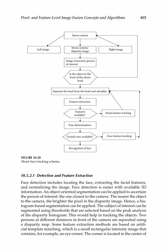
Pixel- and Feature-Level Image Fusion Concepts and Algorithms 405

10.5.2.1 Detection and Feature Extraction

Face detection includes locating the face, extracting the facial features, and normalizing the image. Face detection is easier with available 3D information. An object-oriented segmentation can be applied to ascertain the person of interest: the one closest to the camera. The nearer the object to the camera, the brighter the pixel in the disparity image. Hence, a his-togram-based segmentation can be applied. The subject of interest can be segmented using thresholds that are selected based on the peak analysis of the disparity histogram. This would help in tracking the objects. Two persons at different distances in front of the camera are separated using a disparity map. Some feature extraction methods are based on artifi -cial template matching, which is a small rectangular intensity image that contains, for example, an eye corner. The corner is located in the center of

FIGURE 10.20 Head–face tracking scheme.

Stereo system

Left image Stereo system/disparity image Right image

Image extraction-person-of-interest

Is the object in thefront of the stereo

head

Separate the head from the head-and-shoulder

Feature extraction

Featuresavailable?

Pose determination

Frontal view available?

Recognition of face

Head-feature tracking

Face-feature tracking

406 Multi-Sensor Data Fusion: Theory and Practice

the template. The image region that best matches the artifi cial template is extracted from current image. To apply the corner detector, we need to establish a rectangular search region for the mouth and two rectangular regions for the left and right eyes, respectively.

10.5.2.2 Feature-Level Fusion Using Hand and Face Biometrics

Multibiometric systems use information from multiple biometric sources to verify the identity of an individual, for example, face and fi ngerprints, multiple fi ngers of a user, and multiple matchers [23]. Information from these multiple sources are consolidated into three distinct levels: (1) the feature extraction level, (2) the match score level, and (3) the decision level. Fusion at the feature level is a relatively less attended problem and can be studied in three ways: (1) fusion of PCA and LDA coeffi cients of the face; (2) fusion of LDA coeffi cients corresponding to the R, G, and B channels of a face image; and (3) fusion of face and hand modalities. Thus, multibio-metric systems consolidate the evidence presented by multiple biometric traits or sources. Such systems improve the recognition performance of a biometric system in addition to improving population coverage, deter-ring spoof attacks, increasing the degrees of freedom, and reducing the failure-to-enroll rate. The storage requirements, processing time, and com-putational demands of a multibiometric system are much higher than a monobiometric system.

The information in a multibiometric system can be integrated at the following levels:

1. Sensor level: Data acquired from multiple sensors are processed and integrated in order to generate new data from which fea-tures can be extracted, for example, in the case of face biometrics, both 2D texture information and 3D depth/range information, obtained using two different sensors, can be fused to generate a 3D texture image of the face that is then subjected to feature extraction and matching.

2. Feature level: Feature sets extracted from multiple data sources can be fused to create a new feature set that represents the individual, for example, the geometric features of the hand may be augmented with the eigencoeffi cients of the face to construct a new high-dimensional feature vector. The feature selection and transformation method may be used to elicit a minimal feature set from the high-dimensional feature vector.

3. Match-score level: Multiple classifi ers output a set of match scores that are fused to generate a single scalar score. The match scores generated by the face and hand modalities of a user may be

Pixel- and Feature-Level Image Fusion Concepts and Algorithms 407

combined via the simple sum to obtain a new match score, which is then used to make the fi nal decision.

4. Rank level: This fusion is used in identifi cation systems in which each classifi er associates a rank with every enrolled identity, and a higher rank indicates a good match. The multiple ranks associated with an identity are consolidated and a new rank that would aid in establishing the fi nal decision is determined.

5. Decision level: When each matcher outputs its own class label (i.e., the accept or reject decision in a verifi cation system or the identity of a user in an identifi cation system), a single class label can be obtained by using techniques such as majority voting and behavior knowledge space.

10.5.3 Feature-Level Fusion

Feature-level fusion can be accomplished by linking the feature sets obtained from multiple information sources. Let X = [x

1, x

2, ..., xm ] and

Y = [y1, y

2, ..., ym ] be the feature vectors that represent the information

extracted using two different sources. The fusion of these two sets should give a new feature vector that is generated by fi rst augmenting vectors X and Y , and then performing feature selection on the resultant vector. The process is described in Sections 10.5.3.1 through 10.5.3.3.

10.5.3.1 Feature Normalization

The location (mean) and the scale (variance) of the feature values are modifi ed due to a possible large variation in these values. The minimum–maximum method can give the new value = ( x − min F( x )/(max F( x ) − min F( x )). This requires that the minimum and maximum val-ues be computed beforehand. In the median normalization method, the new value = ( x − median F ( x )/(median (| x − median F ( x )|). The denomi-nator is an estimate of the scale parameter of the feature value. The modi-fi ed feature vectors are subsequently used.

10.5.3.2 Feature Selection

The two normalized feature vectors are put in Z = { X , Y } form. A minimal feature set of size k [ k < ( m + n )] is chosen that enhances the classifi cation performance on a training set of feature vectors. The new feature vector is selected based on the genuine accept rate (GAR) at four levels of false accept rate (FAR) values: 0.05, 0.1, 1, and 10%, in the receiver operating characteristics (ROC) curve related to the training data set.

408 Multi-Sensor Data Fusion: Theory and Practice

10.5.3.3 Match Score Generation

Let there be two composite feature vectors, one at each time instant Z ( t ) and Z ( t + d ), for example, Z = ( X , Y ). Let Sx and Sy be the normalized match (i.e., Euclidean distance) generated by matching each X and Y from the two sets. Then S = ( Sx + Sy )/2 is the fused match score. A distance measure or metric must be computed here.

Once we have the match score level and the feature-level information, we combine them using the simple sum rule to obtain the fi nal score. In the genuine pairs, the high match score would be the effect of a few features’ values that constitute the fused vector. The feature selection process elimi-nates the redundant features and the features that are correlated with the other features. A detailed treatment with results is given in [23].

10.6 Illustrative Examples

The following examples will help in image analysis and image-related fusion exercises, although some of them may not be directly related to image fusion.

EXAMPLE 10.1

Create a current frame and reference object with the following MATLAB® code.

% Current frame Ic = zeros(32,32); Ic(14:21,14:21) = 1; % Reference target/object Ir = ones(7,7); %END of the program

Determine the centroid of the reference object in the current frame using the correlation, sum absolute difference (SAD), and FFT methods.

SOLUTION 10.1 Run the MATLAB code ch10_ex1 . It contains the codes for the correlation, SAD, and FFT methods. The centroid based on (1) correlation is 17.0, 17.0, (2) SAD is 17.0, 17.0, and (3) FFT is 16.0, 17.0.

EXAMPLE 10.2

Compute the coeffi cients (for the transformation function in Equation 10.3) to register two images using the LS method and CPs from the images to be regis-tered. Assume that the CPs from fi rst image are (52.64, 201.66) (261.53, 206.21)

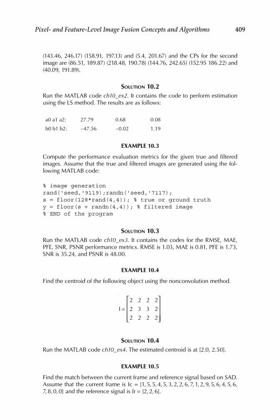
Pixel- and Feature-Level Image Fusion Concepts and Algorithms 409

(143.46, 246.17) (158.91, 197.13) and (5.4, 201.67) and the CPs for the second image are (86.51, 189.87) (218.48, 190.78) (144.76, 242.65) (152.95 186.22) and (40.09, 191.89).

SOLUTION 10.2 Run the MATLAB code ch10_ex2 . It contains the code to perform estimation using the LS method. The results are as follows:

a0 a1 a2: 27.79 0.68 0.08

b0 b1 b2: −47.56 −0.02 1.19

EXAMPLE 10.3

Compute the performance evaluation metrics for the given true and fi ltered images. Assume that the true and fi ltered images are generated using the fol-lowing MATLAB code:

% image generation rand('seed,'9119); randn('seed,'7117); s = floor(128*rand(4,4)); % true or ground truth y = floor(s + randn(4,4)); % filtered image % END of the program

SOLUTION 10.3 Run the MATLAB code ch10_ex3 . It contains the codes for the RMSE, MAE, PFE, SNR, PSNR performance metrics. RMSE is 1.03, MAE is 0.81, PFE is 1.73, SNR is 35.24, and PSNR is 48.00.

EXAMPLE 10.4

Find the centroid of the following object using the nonconvolution method.

I =

2 2 2 2

2 3 3 2

2 2 2 2

⎡

⎣

⎢⎢⎢

⎤

⎦

⎥⎥⎥

SOLUTION 10.4 Run the MATLAB code ch10_ex4 . The estimated centroid is at [2.0, 2.50].

EXAMPLE 10.5

Find the match between the current frame and reference signal based on SAD. Assume that the current frame is Ic = [1, 5, 5, 4, 5, 3, 2, 2, 6, 7, 1, 2, 9, 5, 6, 4, 5, 6, 7, 8, 0, 0] and the reference signal is Ir = [2, 2, 6].

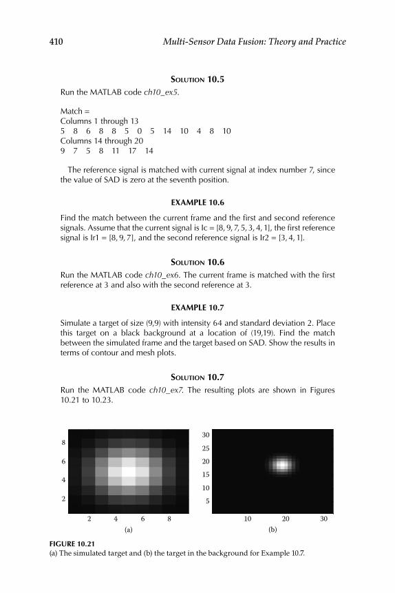
410 Multi-Sensor Data Fusion: Theory and Practice

SOLUTION 10.5 Run the MATLAB code ch10_ex5 .

Match = Columns 1 through 13 5 8 6 8 8 5 0 5 14 10 4 8 10 Columns 14 through 20 9 7 5 8 11 17 14

The reference signal is matched with current signal at index number 7, since the value of SAD is zero at the seventh position.

EXAMPLE 10.6

Find the match between the current frame and the fi rst and second reference signals. Assume that the current signal is Ic = [8, 9, 7, 5, 3, 4, 1], the fi rst reference signal is Ir1 = [8, 9, 7], and the second reference signal is Ir2 = [3, 4, 1].

SOLUTION 10.6 Run the MATLAB code ch10_ex6 . The current frame is matched with the fi rst reference at 3 and also with the second reference at 3.

EXAMPLE 10.7

Simulate a target of size (9,9) with intensity 64 and standard deviation 2. Place this target on a black background at a location of (19,19). Find the match between the simulated frame and the target based on SAD. Show the results in terms of contour and mesh plots.

SOLUTION 10.7 Run the MATLAB code ch10_ex7 . The resulting plots are shown in Figures 10.21 to 10.23.

FIGURE 10.21 (a) The simulated target and (b) the target in the background for Example 10.7.

(b)10 20 30

51015202530

(a)2 4 6 8

2

4

6

8

Pixel- and Feature-Level Image Fusion Concepts and Algorithms 411

EXAMPLE 10.8 Use the data from Example 10.7 and fi nd the match between the simulated frame and the target based on NCC. Show the results in terms of contour and mesh plots.

FIGURE 10.22 (a) The matched image and (b) the mesh for Example 10.7.

10 20 30

5

10

15

20

25

30

(b)0

20

40

0

20

400

0.2

0.4

0.6

0.8

1

(a)

FIGURE 10.23 The contour for Example 10.7.

Contour

5 10 15 20 25 30

5

10

15

20

25

30

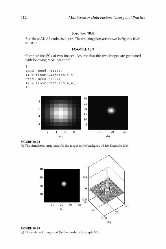
412 Multi-Sensor Data Fusion: Theory and Practice

SOLUTION 10.8 Run the MATLAB code ch10_ex8 . The resulting plots are shown in Figures 10.24 to 10.26.

EXAMPLE 10.9

Compute the PCs of two images. Assume that the two images are generated with following MATLAB code:

% rand('seed,'3443); I1 = floor(128*rand(4,4)); rand('seed,'1991); I2 = floor(128*rand(4,4)); %

FIGURE 10.24 (a) The simulated target and (b) the target in the background for Example 10.8.

(a)2 4 6 8

2

4

6

8

(b)10 20 30

51015202530

FIGURE 10.25 (a) The matched image and (b) the mesh for Example 10.8.

(a)10 20 30 40

10

20

30

40

(b)0

20

40

0

20

40−0.5

0

0.5

1

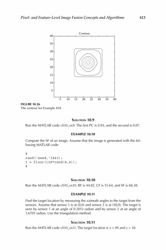
Pixel- and Feature-Level Image Fusion Concepts and Algorithms 413

SOLUTION 10.9 Run the MATLAB code ch10_ex9 . The fi rst PC is 0.93, and the second is 0.07.

EXAMPLE 10.10

Compute the SF of an image. Assume that the image is generated with the fol-lowing MATLAB code:

% rand('seed,'3443); I = floor(128*rand(4,4)); %

SOLUTION 10.10 Run the MATLAB code ch10_ex10 . RF is 44.82, CF is 51.64, and SF is 68.38.

EXAMPLE 10.11

Find the target location by measuring the azimuth angles to the target from the sensors. Assume that sensor 1 is at (0,0) and sensor 2 is at (50,0). The target is seen by sensor 1 at an angle of 0.2013 radian and by sensor 2 at an angle of 1.6705 radian. Use the triangulation method.

SOLUTION 10.11 Run the MATLAB code ch10_ex11 . The target location is x = 49 and y = 10.

FIGURE 10.26 The contour for Example 10.8.

Contour

5 10 15 20 25 30 35 40

5

10

15

20

25

30

35

40

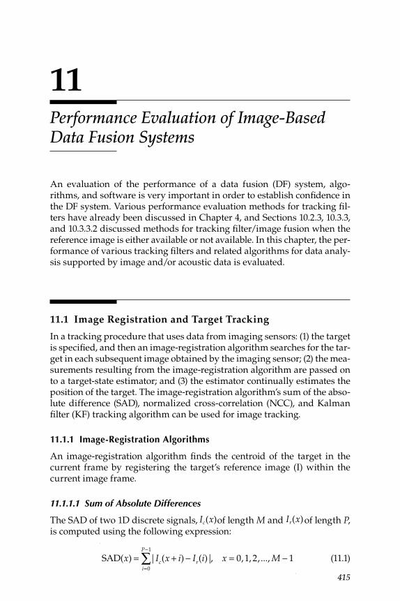
415

11 Performance Evaluation of Image-Based Data Fusion Systems

An evaluation of the performance of a data fusion (DF) system, algo-rithms, and software is very important in order to establish confi dence in the DF system. Various performance evaluation methods for tracking fi l-ters have already been discussed in Chapter 4, and Sections 10.2.3, 10.3.3, and 10.3.3.2 discussed methods for tracking fi lter/image fusion when the reference image is either available or not available. In this chapter, the per-formance of various tracking fi lters and related algorithms for data analy-sis supported by image and/or acoustic data is evaluated.

11.1 Image Registration and Target Tracking

In a tracking procedure that uses data from imaging sensors: (1) the target is specifi ed, and then an image-registration algorithm searches for the tar-get in each subsequent image obtained by the imaging sensor; (2) the mea-surements resulting from the image-registration algorithm are passed on to a target-state estimator; and (3) the estimator continually estimates the position of the target. The image-registration algorithm’s sum of the abso-lute difference (SAD), normalized cross-correlation (NCC), and Kalman fi lter (KF) tracking algorithm can be used for image tracking.

11.1.1 Image-Registration Algorithms

An image-registration algorithm fi nds the centroid of the target in the current frame by registering the target’s reference image (I) within the current image frame.

11.1.1.1 Sum of Absolute Differences

The SAD of two 1D discrete signals, Ic(x)of length M and Ir(x)of length P, is computed using the following expression:

SAD(x) = |Ic(x + i) − Ir(i)|

i=0

P−1

∑ , x = 0,1, 2, ..., M − 1 (11.1)

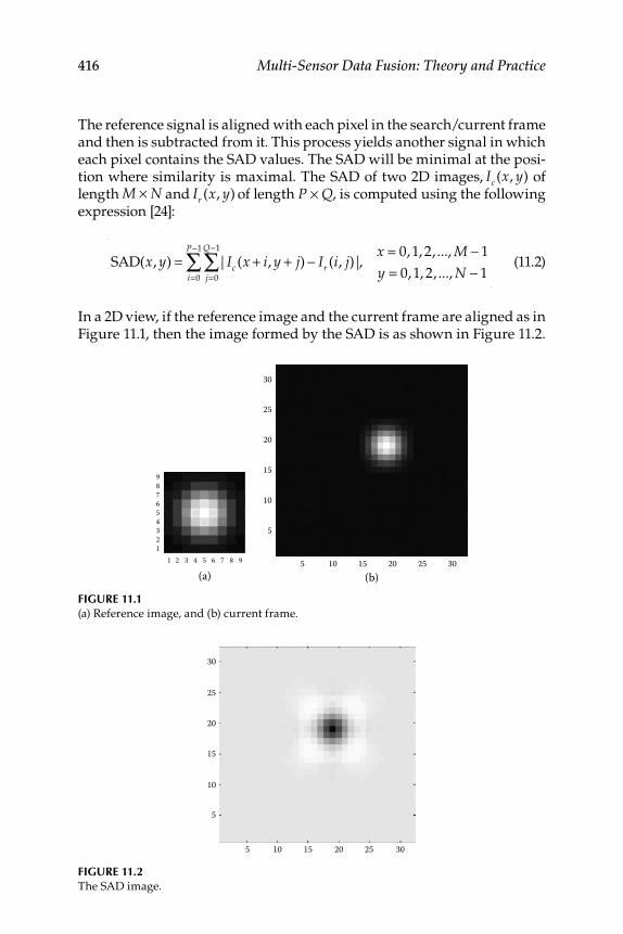
416 Multi-Sensor Data Fusion: Theory and Practice

The reference signal is aligned with each pixel in the search/current frame and then is subtracted from it. This process yields another signal in which each pixel contains the SAD values. The SAD will be minimal at the posi-tion where similarity is maximal. The SAD of two 2D images, Ic (x, y) of length M × N and Ir (x, y) of length P × Q, is computed using the following expression [24]:

SAD(x, y) = |Ic (x + i, y + j) − Ir (i, j)|

j=0

Q−1

∑i=0

P−1

∑ ,x = 0,1, 2, ..., M − 1

y = 0,1, 2, ..., N − 1 (11.2)

In a 2D view, if the reference image and the current frame are aligned as in Figure 11.1, then the image formed by the SAD is as shown in Figure 11.2.

FIGURE 11.1 (a) Reference image, and (b) current frame.

123456789

21 3 4 5 6 7 8 9

(a)

30

25

20

15

10

5

(b)5 10 15 20 25 30

FIGURE 11.2 The SAD image.

30

25

20

15

10

5

5 10 15 20 25 30

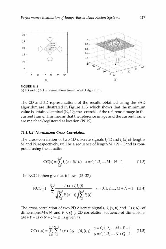
Performance Evaluation of Image-Based Data Fusion Systems 417

The 2D and 3D representations of the results obtained using the SAD algorithm are illustrated in Figure 11.3, which shows that the minimum value is obtained at pixel (19, 19), the centroid of the reference image in the current frame. This means that the reference image and the current frame are matched/registered at location (19, 19).

11.1.1.2 Normalized Cross Correlation

The cross-correlation of two 1D discrete signals Ic (x)and Ir (x) of lengths M and N , respectively, will be a sequence of length M + N − 1and is com-puted using the equation

CC(x) = Ic (x + i)Ir (i)

i=0

N −1

∑ x = 0, 1, 2, ..., M + N − 1 (11.3)

The NCC is then given as follows [25–27]:

NCC(x) =Ic (x + i)Ir (i)

Ic2 (x + i)

i=0

N −1

∑ Ir2 (i)

i=0

N −1

∑i=0

N −1

∑ x = 0, 1, 2, ..., M + N − 1 (11.4)

The cross-correlation of two 2D discrete signals, Ic (x, y) and Ir (x, y), of dimensions M × N and P × Q (a 2D correlation sequence of dimensions (M + P − 1) × (N + Q − 1), is given as

CC(x, y) = Ic (x + i, y + j)Ir (i, j)

j=0

M−1

∑i=0

N −1

∑ x = 0, 1, 2, ..., M + P − 1

y = 0, 1, 2, ..., N + Q − 1 (11.5)

FIGURE 11.3 (a) 2D and (b) 3D representations from the SAD algorithm.

0.40.60.8

1

0.20

(b)00 1010 20

20 3030

4040

30

25

20

15

10

5

(a)5 10 15 20 25 30

X=18Y=19Level=0

X=18Y=19Z=0

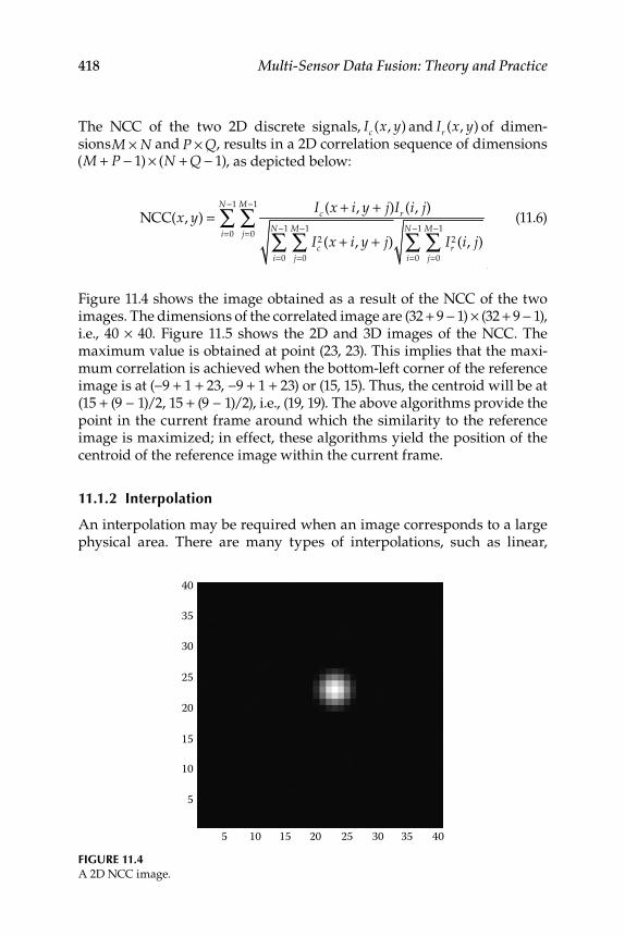
418 Multi-Sensor Data Fusion: Theory and Practice

The NCC of the two 2D discrete signals, Ic (x, y) and Ir (x, y) of dimen-sionsM × N and P × Q, results in a 2D correlation sequence of dimensions(M + P − 1) × (N + Q − 1), as depicted below:

NCC(x, y) =Ic (x + i, y + j)Ir (i, j)

Ic2 (x + i, y + j)

j=0

M−1

∑i=0

N −1

∑ Ir2 (i, j)

j=0

M−1

∑i=0

N −1

∑j=0

M−1

∑i=0

N −1

∑ (11.6)

Figure 11.4 shows the image obtained as a result of the NCC of the two images. The dimensions of the correlated image are (32 + 9 − 1) × (32 + 9 − 1), i.e., 40 × 40. Figure 11.5 shows the 2D and 3D images of the NCC. The maximum value is obtained at point (23, 23). This implies that the maxi-mum correlation is achieved when the bottom-left corner of the reference image is at (−9 + 1 + 23, −9 + 1 + 23) or (15, 15). Thus, the centroid will be at (15 + (9 − 1)/2, 15 + (9 − 1)/2), i.e., (19, 19). The above algorithms provide the point in the current frame around which the similarity to the reference image is maximized; in effect, these algorithms yield the position of the centroid of the reference image within the current frame.

11.1.2 Interpolation

An interpolation may be required when an image corresponds to a large physical area. There are many types of interpolations, such as linear,

FIGURE 11.4 A 2D NCC image.

30

35

40

25

20

15

10

5

5 10 15 20 25 30 35 40

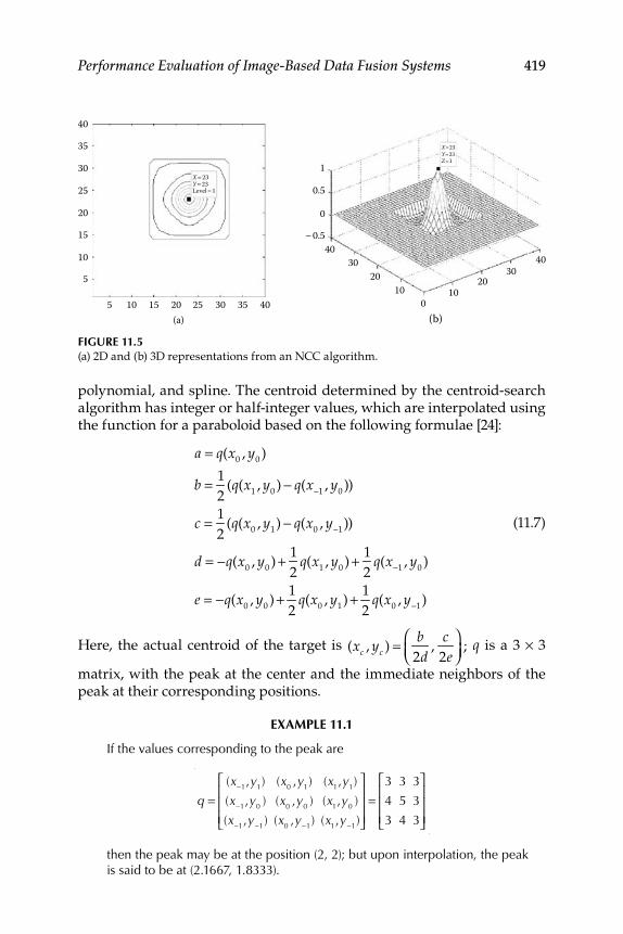
Performance Evaluation of Image-Based Data Fusion Systems 419

polynomial, and spline. The centroid determined by the centroid-search algorithm has integer or half-integer values, which are interpolated using the function for a paraboloid based on the following formulae [24]:

a = q(x0, y

0)

b = 1

2(q(x

1, y

0) − q(x−1

, y0))

c = 1

2(q(x

0, y

1) − q(x

0, y−1

))

d = −q(x0, y

0) + 1

2q(x

1, y

0) + 1

2q(x−1

, y0)

e = −q(x0, y

0) + 1

2q(x

0, y

1) + 1

2q(x

0, y−1

)

(11.7)

Here, the actual centroid of the target is (xc , yc ) = b2d

,c

2e⎛⎝⎜

⎞⎠⎟

; q is a 3 × 3

matrix, with the peak at the center and the immediate neighbors of the peak at their corresponding positions.

EXAMPLE 11.1

If the values corresponding to the peak are

q =(x−1,y1) (x0 ,y1) (x1,y1)

(x−1,y0 ) (x0 ,y0 ) (x1,y0 )

(x−1,y−1) (x0 ,y−1) (x1,y−1)

⎡

⎣

⎢⎢⎢

⎤

⎦

⎥⎥⎥

=3 3 3

4 5 3

3 4 3

⎡

⎣

⎢⎢⎢

⎤

⎦

⎥⎥⎥

then the peak may be at the position (2, 2); but upon interpolation, the peak is said to be at (2.1667, 1.8333).

FIGURE 11.5 (a) 2D and (b) 3D representations from an NCC algorithm.

-0.5

0

0.5

1

(b)0

10102020 30

3040

40

30

35

40

25

20

15

10

5

(a)5 10 15 20 25 30 35 40

X=23Y=23Level=1

X=23Y=23Z=1

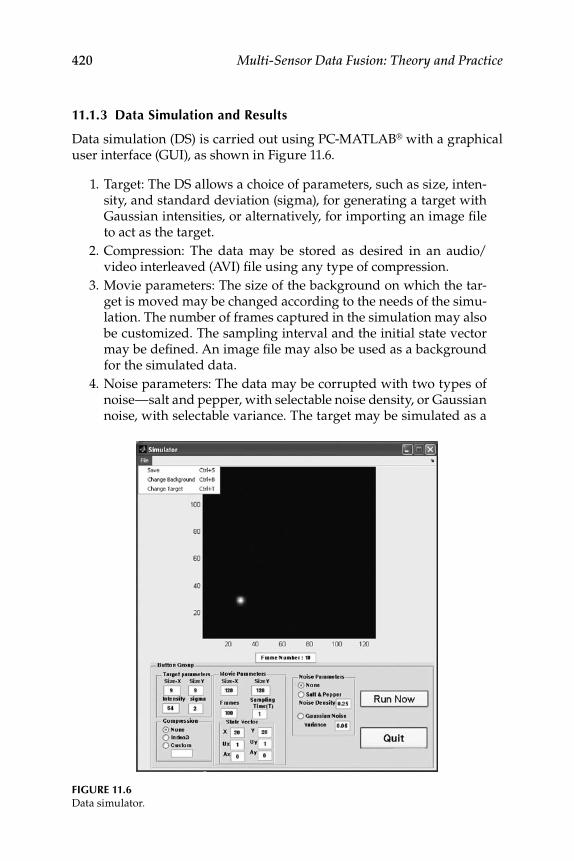
420 Multi-Sensor Data Fusion: Theory and Practice

11.1.3 Data Simulation and Results

Data simulation (DS) is carried out using PC-MATLAB® with a graphical user interface (GUI), as shown in Figure 11.6.

1. Target: The DS allows a choice of parameters, such as size, inten-sity, and standard deviation (sigma), for generating a target with Gaussian intensities, or alternatively, for importing an image fi le to act as the target.

2. Compression: The data may be stored as desired in an audio/video interleaved (AVI) fi le using any type of compression.

3. Movie parameters: The size of the background on which the tar-get is moved may be changed according to the needs of the simu-lation. The number of frames captured in the simulation may also be customized. The sampling interval and the initial state vector may be defi ned. An image fi le may also be used as a background for the simulated data.

4. Noise parameters: The data may be corrupted with two types of noise—salt and pepper, with selectable noise density, or Gaussian noise, with selectable variance. The target may be simulated as a

FIGURE 11.6 Data simulator.

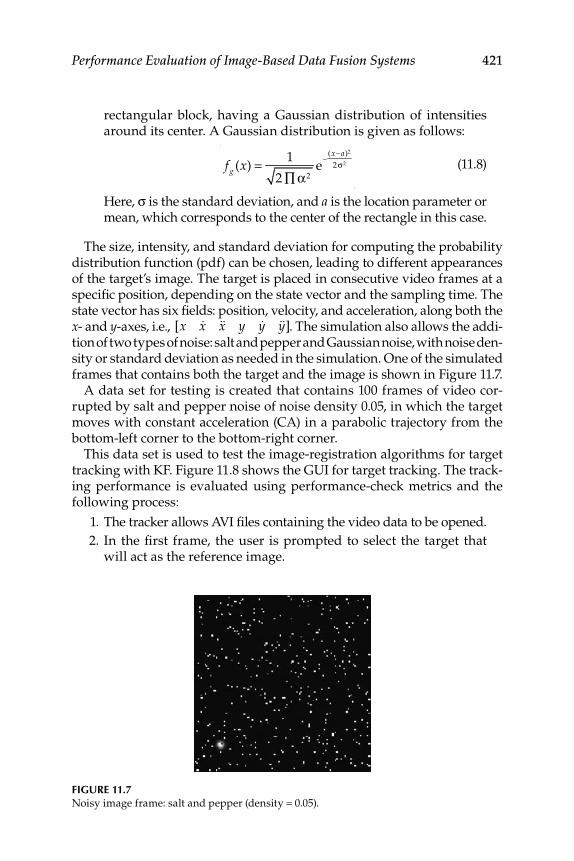
Performance Evaluation of Image-Based Data Fusion Systems 421

rectangular block, having a Gaussian distribution of intensities around its center. A Gaussian distribution is given as follows:

fg (x) = 1

2 ∏ α2e

−(x−a)2

2σ2 (11.8)

Here, σ is the standard deviation, and a is the location parameter or mean, which corresponds to the center of the rectangle in this case.

The size, intensity, and standard deviation for computing the probability distribution function (pdf) can be chosen, leading to different appearances of the target’s image. The target is placed in consecutive video frames at a specifi c position, depending on the state vector and the sampling time. The state vector has six fi elds: position, velocity, and acceleration, along both the x - and y -axes, i.e., [x &x &&x y &y &&y]. The simulation also allows the addi-tion of two types of noise: salt and pepper and Gaussian noise, with noise den-sity or standard deviation as needed in the simulation. One of the simulated frames that contains both the target and the image is shown in Figure 11.7.

A data set for testing is created that contains 100 frames of video cor-rupted by salt and pepper noise of noise density 0.05, in which the target moves with constant acceleration (CA) in a parabolic trajectory from the bottom-left corner to the bottom-right corner.

This data set is used to test the image-registration algorithms for target tracking with KF. Figure 11.8 shows the GUI for target tracking. The track-ing performance is evaluated using performance-check metrics and the following process:

1. The tracker allows AVI fi les containing the video data to be opened.

2. In the fi rst frame, the user is prompted to select the target that will act as the reference image.

FIGURE 11.7 Noisy image frame: salt and pepper (density = 0.05).

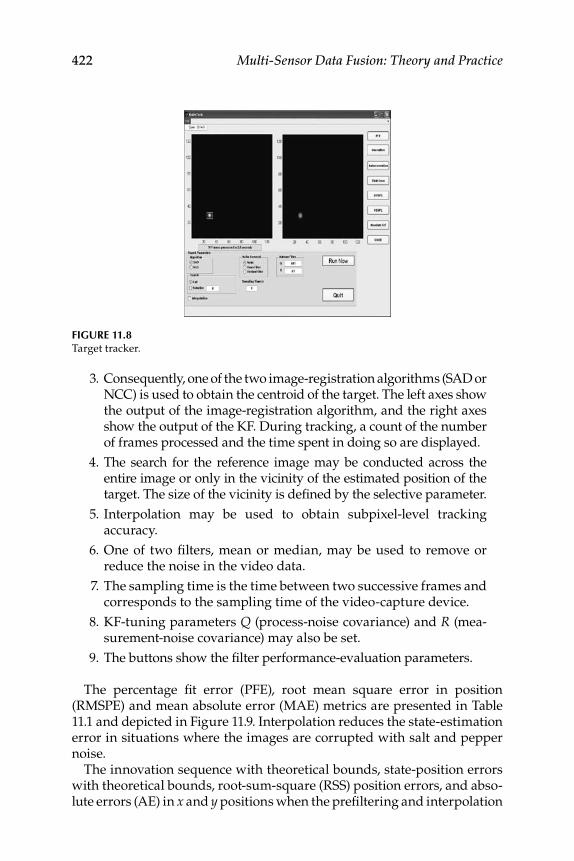
422 Multi-Sensor Data Fusion: Theory and Practice

3. Consequently, one of the two image-registration algorithms (SAD or NCC) is used to obtain the centroid of the target. The left axes show the output of the image- registration algorithm, and the right axes show the output of the KF. During tracking, a count of the number of frames processed and the time spent in doing so are displayed.

4. The search for the reference image may be conducted across the entire image or only in the vicinity of the estimated position of the target. The size of the vicinity is defi ned by the selective parameter.

5. Interpolation may be used to obtain subpixel-level tracking accuracy.

6. One of two fi lters, mean or median, may be used to remove or reduce the noise in the video data.

7. The sampling time is the time between two successive frames and corresponds to the sampling time of the video- capture device.

8. KF-tuning parameters Q (process-noise covariance) and R (mea-surement-noise covariance) may also be set.

9. The buttons show the fi lter performance- evaluation parameters.

The percentage fi t error (PFE), root mean square error in position (RMSPE) and mean absolute error (MAE) metrics are presented in Table 11.1 and depicted in Figure 11.9. Interpolation reduces the state-estimation error in situations where the images are corrupted with salt and pepper noise.

The innovation sequence with theoretical bounds, state-position errors with theoretical bounds, root-sum-square (RSS) position errors, and abso-lute errors (AE) in x and y positions when the prefi ltering and interpolation

FIGURE 11.8 Target tracker.

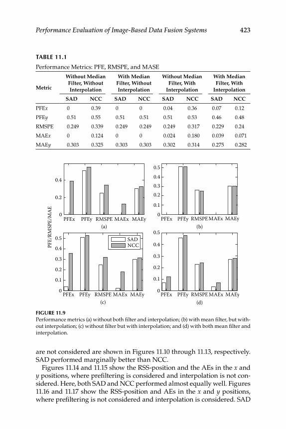
Performance Evaluation of Image-Based Data Fusion Systems 423

are not considered are shown in Figures 11.10 through 11.13, respectively. SAD performed marginally better than NCC.

Figures 11.14 and 11.15 show the RSS-position and the AEs in the x and y positions, where prefi ltering is considered and interpolation is not con-sidered. Here, both SAD and NCC performed almost equally well. Figures 11.16 and 11.17 show the RSS-position and AEs in the x and y positions, where prefi ltering is not considered and interpolation is considered. SAD

TABLE 11.1

Performance Metrics: PFE, RMSPE, and MASE

Metric

Without Median

Filter, Without

Interpolation

With Median

Filter, Without

Interpolation

Without Median

Filter, With

Interpolation

With Median

Filter, With

Interpolation

SAD NCC SAD NCC SAD NCC SAD NCC

PFEx 0 0.39 0 0 0.04 0.36 0.07 0.12

PFEy 0.51 0.55 0.51 0.51 0.51 0.53 0.46 0.48

RMSPE 0.249 0.339 0.249 0.249 0.249 0.317 0.229 0.24

MAEx 0 0.124 0 0 0.024 0.180 0.039 0.071

MAEy 0.303 0.325 0.303 0.303 0.302 0.314 0.275 0.282

FIGURE 11.9 Performance metrics (a) without both fi lter and interpolation; (b) with mean fi lter, but with-

out interpolation; (c) without fi lter but with interpolation; and (d) with both mean fi lter and

interpolation.

0.5

0.40.30.2

0.1

0PFEx PFEy

PFEy

RMSPE(b)

MAEx MAEy

PFEx RMSPE(d)

MAEx MAEyPFEyPFEx RMSPE(c)

MAEx MAEy

PFEyPFEx RMSPE(a)

MAEx MAEy

SAD

PFE/

RMSP

E/M

AE

NCC

0.4

0.2

0

0.5

0.4

0.3

0.2

0.1

0

0.5

0.4

0.3

0.2

0.1

0

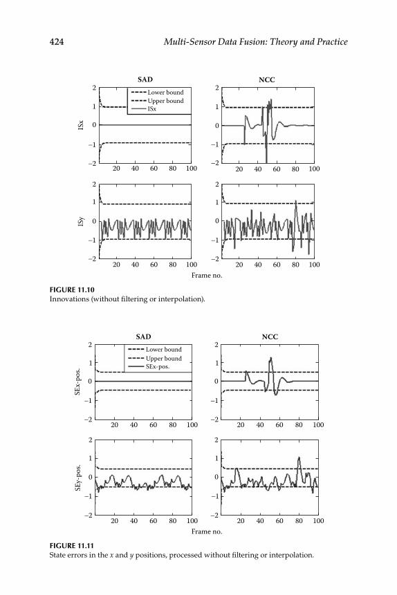
424 Multi-Sensor Data Fusion: Theory and Practice

FIGURE 11.10 Innovations (without fi ltering or interpolation).

2

1

-1

-2

0

20 40 60 80 100

ISy

SADLower boundUpper boundISx

NCC2

1

-1

-2

0ISx

20 40 60 80 100

2

1

-1

-2

0

20 40 60 80 100

2

1

-1

-2

0

20 40 60 80 100Frame no.

FIGURE 11.11 State errors in the x and y positions, processed without fi ltering or interpolation.

2

1

-1

-2

0

SEx-

pos.

SEy-

pos.

20 40

SADLower boundUpper boundSEx-pos.

NCC

60 80 100

2

1

-1

-2

0

20 40 60 80 100Frame no.

20 40 60 80 100

2

1

-1

-2

0

20 40 60 80 100

2

1

-1

-2

0

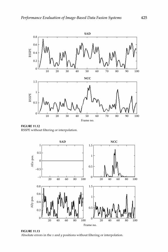
Performance Evaluation of Image-Based Data Fusion Systems 425

FIGURE 11.13 Absolute errors in the x and y positions without fi ltering or interpolation.

20 40 60 80 100

1

0.5

-0.5

-1

0

AEx-

pos.

AEy-

pos.

20 40

SAD NCC

60 80 100

0.8

0.6

0.4

0.2

0

1.5

1

0.5

0

1.5

1

0.5

0

20 40 60 80 100 20 40 60 80 100Frame no.

FIGURE 11.12 RSSPE without fi ltering or interpolation.

SAD

NCC

RSSP

ERS

SPE

2010 30 40 50Frame no.

60 70 9080 100

2010

0.8

0.6

0.4

0.2

1.5

1

0.5

0

030 40 50 60 70 9080 100

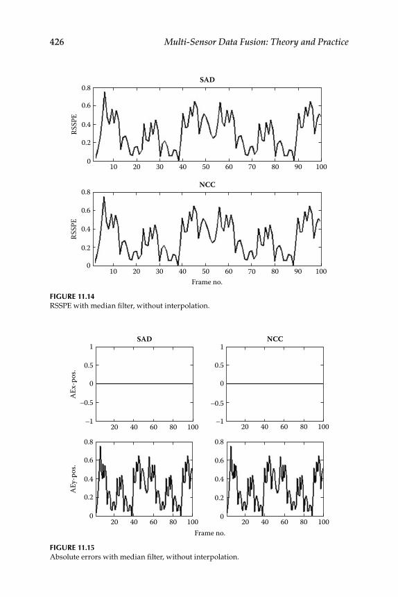
426 Multi-Sensor Data Fusion: Theory and Practice

FIGURE 11.14 RSSPE with median fi lter, without interpolation.

SAD

NCC

RSSP

E

2010 30 40 50Frame no.

60 70 9080 100

2010

0.8

0.6

0.4

0.2

0

RSSP

E

0.8

0.6

0.4

0.2

0

30 40 50 60 70 9080 100

FIGURE 11.15 Absolute errors with median fi lter, without interpolation.

1

0.5

-0.5

-1

0

1

0.5

-0.5

-1

0

20 40 60 80 100

AEx-

pos.

AEy-

pos.

20 40

SAD NCC

60 80 100

20 40 60 80 100

0.8

0.6

0.4

0.2

0

0.8

0.6

0.4

0.2

020 40 60 80 100

Frame no.

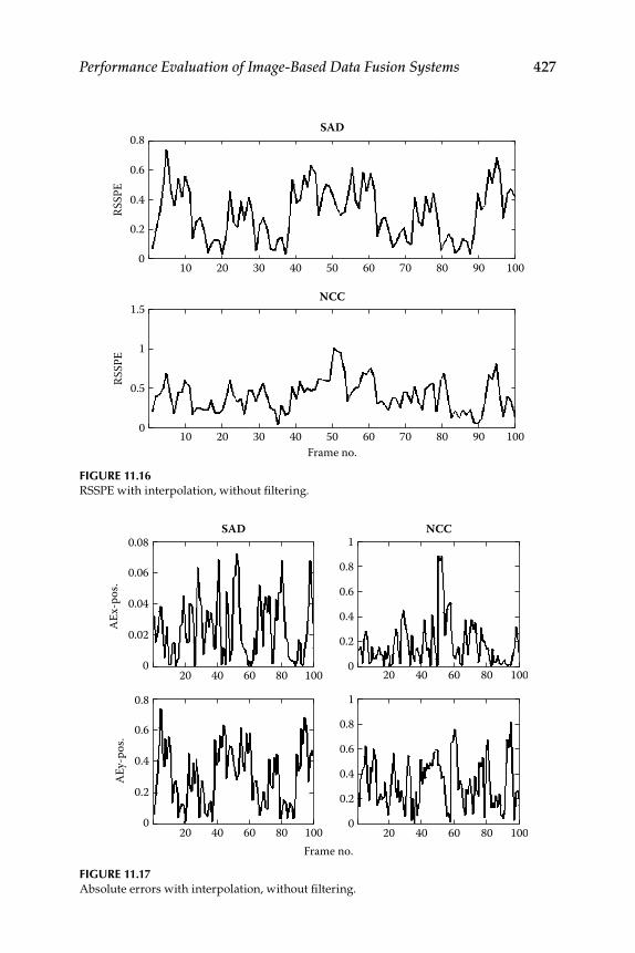
Performance Evaluation of Image-Based Data Fusion Systems 427

FIGURE 11.17 Absolute errors with interpolation, without fi ltering.

20 40 60

SAD NCC

80 100 20 40 60 80 100

20 40 60 80 100

0.08

AEx-

pos.

0.06

0.04

0.02

0

20 40 60 80 100Frame no.

AEy-

pos.

0.8

0.6

0.4

0.2

0

1

0.8

0.6

0.4

0.2

0

1

0.8

0.6

0.4

0.2

0

FIGURE 11.16 RSSPE with interpolation, without fi ltering.

0.8SAD

NCC

Frame no.

RSSP

ERS

SPE

0.6

0.4

0.2

010 20 30 40 50 60 70 80 90 100

0

0.5

1

1.5

10 20 30 40 50 60 70 80 90 100

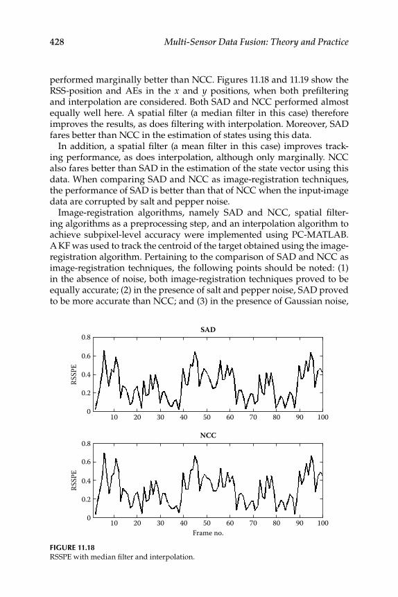
428 Multi-Sensor Data Fusion: Theory and Practice

performed marginally better than NCC. Figures 11.18 and 11.19 show the RSS-position and AEs in the x and y positions, when both prefi ltering and interpolation are considered. Both SAD and NCC performed almost equally well here. A spatial fi lter (a median fi lter in this case) therefore improves the results, as does fi ltering with interpolation. Moreover, SAD fares better than NCC in the estimation of states using this data.

In addition, a spatial fi lter (a mean fi lter in this case) improves track-ing performance, as does interpolation, although only marginally. NCC also fares better than SAD in the estimation of the state vector using this data. When comparing SAD and NCC as image-registration techniques, the performance of SAD is better than that of NCC when the input-image data are corrupted by salt and pepper noise.

Image-registration algorithms, namely SAD and NCC, spatial fi lter-ing algorithms as a preprocessing step, and an interpolation algorithm to achieve subpixel-level accuracy were implemented using PC-MATLAB. A KF was used to track the centroid of the target obtained using the image-registration algorithm. Pertaining to the comparison of SAD and NCC as image-registration techniques, the following points should be noted: (1) in the absence of noise, both image-registration techniques proved to be equally accurate; (2) in the presence of salt and pepper noise, SAD proved to be more accurate than NCC; and (3) in the presence of Gaussian noise,

FIGURE 11.18 RSSPE with median fi lter and interpolation.

0.8SAD

NCC

Frame no.

RSSP

ERS

SPE

0.6

0.4

0.2

0

0.8

0.6

0.4

0.2

0

10 20 30 40 50 60 70 80 90 100

10 20 30 40 50 60 70 80 90 100

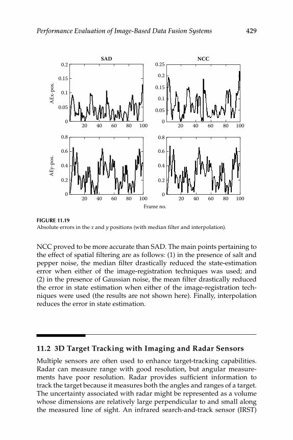
Performance Evaluation of Image-Based Data Fusion Systems 429

NCC proved to be more accurate than SAD. The main points pertaining to the effect of spatial fi ltering are as follows: (1) in the presence of salt and pepper noise, the median fi lter drastically reduced the state- estimation error when either of the image-registration techniques was used; and (2) in the presence of Gaussian noise, the mean fi lter drastically reduced the error in state estimation when either of the image-registration tech-niques were used (the results are not shown here). Finally, interpolation reduces the error in state estimation.

11.2 3D Target Tracking with Imaging and Radar Sensors

Multiple sensors are often used to enhance target-tracking capabilities. Radar can measure range with good resolution, but angular measure-ments have poor resolution. Radar provides suffi cient information to track the target because it measures both the angles and ranges of a target. The uncertainty associated with radar might be represented as a volume whose dimensions are relatively large perpendicular to and small along the measured line of sight. An infrared search-and-track sensor (IRST)

FIGURE 11.19 Absolute errors in the x and y positions (with median fi lter and interpolation) .

20 40 60

SAD NCC

80 100 20 40 60 80 100

20 40 60 80 100

0.2

AEx-

pos.

0.15

0.1

0.05

0

20 40 60 80 100Frame no.

AEy-

pos.

0.8

0.6

0.4

0.2

0

0.8

0.6

0.4

0.2

0

0.25

0.2

0.15

0.1

0.05

0

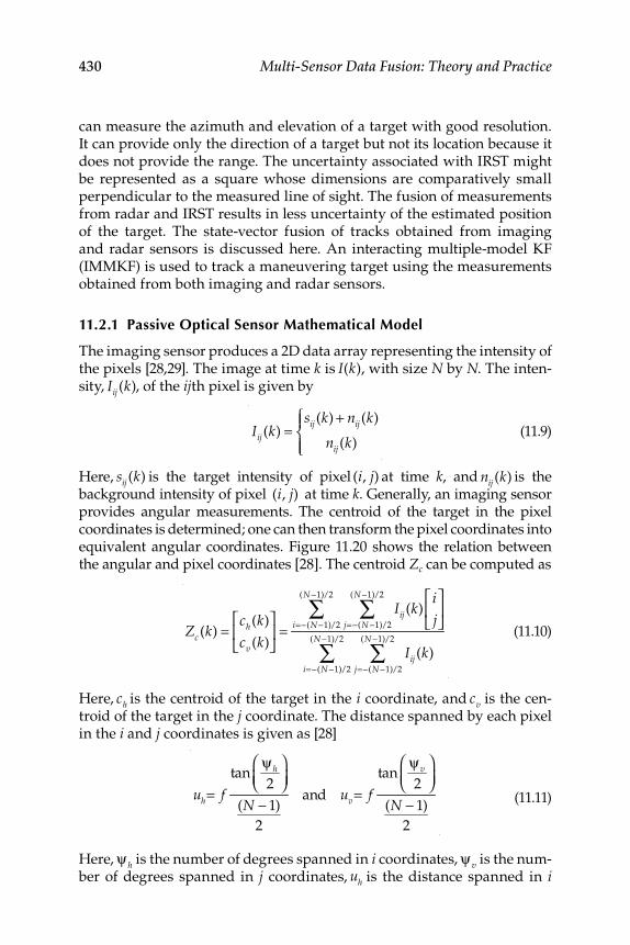
430 Multi-Sensor Data Fusion: Theory and Practice

can measure the azimuth and elevation of a target with good resolution. It can provide only the direction of a target but not its location because it does not provide the range. The uncertainty associated with IRST might be represented as a square whose dimensions are comparatively small perpendicular to the measured line of sight. The fusion of measurements from radar and IRST results in less uncertainty of the estimated position of the target. The state-vector fusion of tracks obtained from imaging and radar sensors is discussed here. An interacting multiple-model KF (IMMKF) is used to track a maneuvering target using the measurements obtained from both imaging and radar sensors.

11.2.1 Passive Optical Sensor Mathematical Model

The imaging sensor produces a 2D data array representing the intensity of the pixels [28,29]. The image at time k is I(k), with size N by N . The inten-sity, Iij (k), of the ij th pixel is given by

Iij (k) =sij (k) + nij (k)

nij (k)

⎧⎨⎪

⎩⎪ (11.9)

Here, sij (k) is the target intensity of pixel (i, j) at time k , and nij (k) is the background intensity of pixel (i, j) at time k . Generally, an imaging sensor provides angular measurements. The centroid of the target in the pixel coordinates is determined; one can then transform the pixel coordinates into equivalent angular coordinates. Figure 11.20 shows the relation between the angular and pixel coordinates [28]. The centroid Zc can be computed as

Zc (k) =ch(k)

cv (k)

⎡

⎣⎢

⎤

⎦⎥ =

Iij (k)i

j

⎡

⎣⎢

⎤

⎦⎥

j=−(N −1)/2

(N −1)/2

∑i=−(N −1)/2

(N −1)/2

∑

Iij (k)j=−(N −1)/2

(N −1)/2

∑i=−(N −1)/2

(N −1)/2

∑ (11.10)

Here, ch is the centroid of the target in the i coordinate, and cv is the cen-troid of the target in the j coordinate. The distance spanned by each pixel in the i and j coordinates is given as [28]

uh= f

tanψ h

2

⎛⎝⎜

⎞⎠⎟

(N − 1)

2

and uv= f

tanψ v

2

⎛⎝⎜

⎞⎠⎟

(N − 1)

2

(11.11)

Here, ψ h is the number of degrees spanned in i coordinates, ψ v is the num-ber of degrees spanned in j coordinates, uh is the distance spanned in i

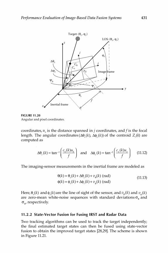
Performance Evaluation of Image-Based Data Fusion Systems 431

coordinates, uv is the distance spanned in j coordinates, and f is the focal length. The angular coordinates (Δθc(k), Δφc(k)) of the centroid Zc(k) are computed as

Δθc (k) = tan−1

ch(k)uh

f⎛⎝⎜

⎞⎠⎟

and Δφc (k) = tan−1cv (k)uv

f⎛⎝⎜

⎞⎠⎟

(11.12)

The imaging-sensor measurements in the inertial frame are modeled as

θ(k) = θs(k) + Δθc(k) + vθ(k) (rad)

φ(k) = φs(k) + Δφc(k) + vφ(k) (rad) (11.13)

Here, θs(k) and φs(k) are the line of sight of the sensor, and vθ(k) and vφ(k)are zero-mean white-noise sequences with standard deviations σθ and σφ, respectively.

11.2.2 State-Vector Fusion for Fusing IRST and Radar Data

Two tracking algorithms can be used to track the target independently; the fi nal estimated target states can then be fused using state-vector fusion to obtain the improved target states [28,29]. The scheme is shown in Figure 11.21.

FIGURE 11.20 Angular and pixel coordinates.

ϕs

y

x

z

i

j

oij

Target: (θc , ϕc)LOS: (θs , ϕs)

θs

Δθc

Δϕc

Ψh

Ψv

ChCv

Inertial frame

Image frame

f

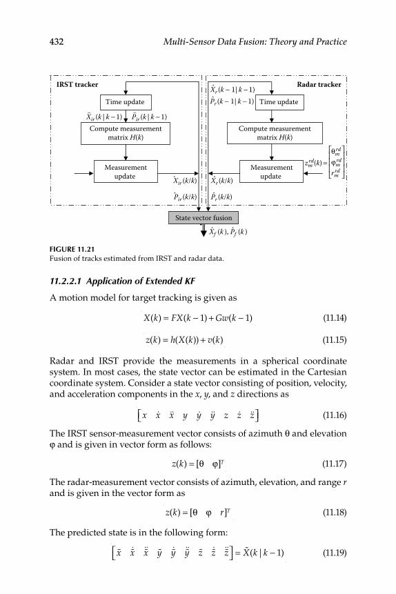
432 Multi-Sensor Data Fusion: Theory and Practice

11.2.2.1 Application of Extended KF

A motion model for target tracking is given as

X(k) = FX(k − 1) + Gw(k − 1) (11.14)

z(k) = h(X(k)) + v(k) (11.15)

Radar and IRST provide the measurements in a spherical coordinate system. In most cases, the state vector can be estimated in the Cartesian coordinate system. Consider a state vector consisting of position, velocity, and acceleration components in the x , y , and z directions as

x &x &&x y &y &&y z &z &&z⎡⎣ ⎤⎦ (11.16)

The IRST sensor-measurement vector consists of azimuth θ and elevation ϕ and is given in vector form as follows:

z(k) = [θ ϕ]T (11.17)

The radar-measurement vector consists of azimuth, elevation, and range r and is given in the vector form as

z(k) = [θ ϕ r]T (11.18)

The predicted state is in the following form:

%x %&x %&&x %y %&y %&&y %z %&z %&&z⎡⎣ ⎤⎦ = %X(k|k − 1) (11.19)

FIGURE 11.21 Fusion of tracks estimated from IRST and radar data.

Radar tracker IRST tracker

Time update Time update

Compute measurementmatrix H(k)

Compute measurementmatrix H(k)

Measurementupdate

Measurementupdate

State vector fusion

Xir (k | k − 1)

zmrd(k) =

θmrd

ϕmrd

rmrd

~

Xir (k/k)ˆ

Pir (k/k)ˆ

Xr (k − 1| k − 1)ˆ

Pr (k − 1| k − 1)ˆ

Xr (k/k)ˆ

Xf (k ), Pf (k )ˆ ˆ

Pr (k/k)ˆ

Pir (k | k − 1)~

⎡⎢⎢⎢⎣

⎡⎢⎢⎢⎣

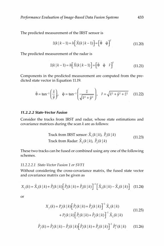
Performance Evaluation of Image-Based Data Fusion Systems 433

The predicted measurement of the IRST sensor is

%z(k|k − 1) = h %X(k|k − 1)⎡⎣ ⎤⎦ = %θ %ϕ⎡⎣ ⎤⎦

T

(11.20)

The predicted measurement of the radar is

%z(k|k − 1) = h %X(k|k − 1)⎡⎣ ⎤⎦ = %θ %ϕ %r⎡⎣ ⎤⎦

T

(11.21)

Components in the predicted measurement are computed from the pre-dicted state vector in Equation 11.19.

%θ = tan−1%x%y

⎛⎝⎜

⎞⎠⎟

, %ϕ = tan−1%z

%x2 + %y2

⎛

⎝⎜

⎞

⎠⎟ , %r = %x2 + %y2 + %z2 (11.22)

11.2.2.2 State-Vector Fusion

Consider the tracks from IRST and radar, whose state estimations and covariance matrices during the scan k are as follows:

Track from IRST sensor: X1(k|k), P

1(k|k)

Track from Radar: X2(k|k), P

2(k|k)

(11.23)

These two tracks can be fused or combined using any one of the following schemes.

11.2.2.2.1 State-Vector Fusion 1 or SVF1

Without considering the cross-covariance matrix, the fused state vector and covariance matrix can be given as

X f (k) = X

1(k|k) + P

1(k|k) P

1(k|k) + P

2(k|k)⎡⎣ ⎤⎦

−1

X2(k|k) − X

1(k|k)⎡⎣ ⎤⎦ (11.24)

or

X f (k) = P

2(k|k) P

1(k|k) + P

2(k|k)⎡⎣ ⎤⎦

−1

X1(k|k)

+ P1(k|k) P

1(k|k) + P

2(k|k)⎡⎣ ⎤⎦

−1

X2(k|k)

(11.25)

Pf (k) = P

1(k|k) − P

1(k|k) P

1(k|k) + P

2(k|k)⎡⎣ ⎤⎦

−1

P1T (k|k) (11.26)

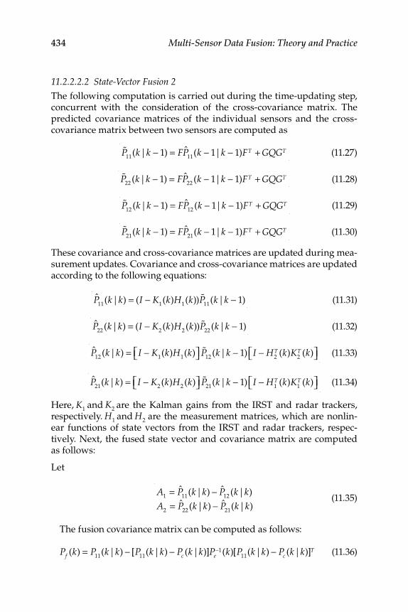
434 Multi-Sensor Data Fusion: Theory and Practice

11.2.2.2.2 State-Vector Fusion 2

The following computation is carried out during the time-updating step, concurrent with the consideration of the cross-covariance matrix. The predicted covariance matrices of the individual sensors and the cross- covariance matrix between two sensors are computed as

%P11

(k|k − 1) = FP11

(k − 1|k − 1)FT + GQGT (11.27)

%P22

(k|k − 1) = FP22

(k − 1|k − 1)FT + GQGT (11.28)

%P12

(k|k − 1) = FP12

(k − 1|k − 1)FT + GQGT (11.29)

%P21

(k|k − 1) = FP21

(k − 1|k − 1)FT + GQGT (11.30)

These covariance and cross-covariance matrices are updated during mea-surement updates. Covariance and cross-covariance matrices are updated according to the following equations:

P11(k|k) = (I − K

1(k)H

1(k)) %P

11(k|k − 1) (11.31)

P22(k|k) = (I − K

2(k)H

2(k)) %P

22(k|k − 1) (11.32)

P

12(k|k) = I − K

1(k)H

1(k)⎡⎣ ⎤⎦ %P

12(k|k − 1) I − H

2T (k)K

2T (k)⎡⎣ ⎤⎦ (11.33)

P

21(k|k) = I − K

2(k)H

2(k)⎡⎣ ⎤⎦ %P

21(k|k − 1) I − H

1T (k)K

1T (k)⎡⎣ ⎤⎦ (11.34)

Here, K1and K

2 are the Kalman gains from the IRST and radar trackers, respectively. H

1 and H2 are the measurement matrices, which are nonlin-

ear functions of state vectors from the IRST and radar trackers, respec-tively. Next, the fused state vector and covariance matrix are computed as follows:

Let

A1

= P11

(k|k) − P12

(k|k)

A2

= P22

(k|k) − P21

(k|k)

(11.35)

The fusion covariance matrix can be computed as follows:

Pf (k) = P11

(k|k) − [P11

(k|k) − Pc (k|k)]Pe−1(k)[P

11(k|k) − Pc (k|k)]T (11.36)

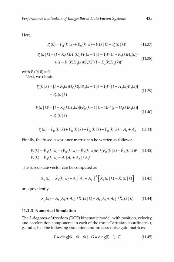
Performance Evaluation of Image-Based Data Fusion Systems 435

Here,

Pe (k) = P

11(k|k) + P

22(k|k) − Pc (k|k) − Pc (k|k)T (11.37)

Pc (k|k) = (I − K

1(k)H

1(k))FPc(k − 1|k − 1)FT(I − K

2(k)H

2(k))

+ (I − K1(k)H

1(k))GQGT(I − K

2(k)H

2(k))T

(11.38)

with Pc (0|0) = 0. Next, we obtain

Pc(k|k) = [I − K1(k)H

1(k)]F %P

12(k − 1|k − 1)FT [I − H

2(k)K

2(k)]

= P

12(k|k)

(11.39)

Pc(k|k)T = [I − K2(k)H

2(k)]F %P

21(k − 1|k − 1)FT [I − H

1(k)K

1(k)]

= P

21(k|k)

(11.40)

Pe (k) = P

11(k|k) + P

22(k|k) − P

12(k|k) − P

21(k|k) = A

1+ A

2 (11.41)

Finally, the fused covariance matrix can be written as follows:

Pf (k) = P11

(k|k) − (P11

(k|k) − P12

(k|k))Pe−1(P

11(k|k) − P

12(k|k))T

Pf (k) = P11

(k|k) − A1[A

1+ A

2]−1 A

1T

(11.42)

The fused state vector can be computed as

X f (k) = X

1(k|k) + A

1A

1+ A

2⎡⎣ ⎤⎦

−1X

2(k|k) − X

1(k|k)⎡⎣ ⎤⎦ (11.43)

or equivalently

X f (k) = A

2[A

1+ A

2]−1 X

1(k|k) + A

1[A

1+ A

2]−1 X

2(k|k) (11.44)

11.2.3 Numerical Simulation

The 3-degrees-of-freedom (DOF) kinematic model, with position, velocity, and acceleration components in each of the three Cartesian coordinates x , y , and z , has the following transition and process-noise gain matrices:

F = diag[Φ Φ Φ] G = diag[ζ ζ ζ] (11.45)

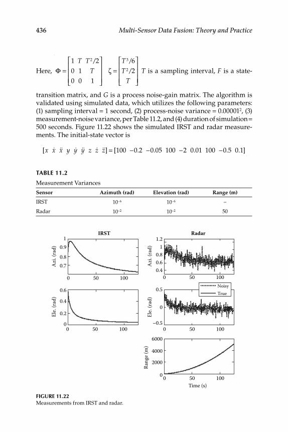
436 Multi-Sensor Data Fusion: Theory and Practice

Here,

Φ =1 T T 2/2

0 1 T

0 0 1

⎡

⎣

⎢⎢⎢

⎤

⎦

⎥⎥⎥

ζ =T 3/6

T 2/2

T

⎡

⎣

⎢⎢⎢

⎤

⎦

⎥⎥⎥

T is a sampling interval, F is a state-

transition matrix, and G is a process noise-gain matrix. The algorithm is validated using simulated data, which utilizes the following parameters: (1) sampling interval = 1 second, (2) process-noise variance = 0.00001 2 , (3) measurement-noise variance, per Table 11.2, and (4) duration of simulation = 500 seconds. Figure 11.22 shows the simulated IRST and radar measure-ments. The initial-state vector is

[x &x &&x y &y &&y z &z &&z] = [100 −0.2 −0.05 100 −2 0.01 100 −0.5 0.1]

TABLE 11.2

Measurement Variances

Sensor Azimuth (rad) Elevation (rad) Range (m)

IRST 10−6 10−6 –

Radar 10−2 10−2 50

FIGURE 11.22Measurements from IRST and radar.

IRST1

0.90.80.7

0 50 100

0 50 100

0 50 100

0 50 100

0 50 100

Azi. (

rad)

Radar1.2

1

0.60.8

0.4

Azi. (

rad)

0.5

0

–0.5

6000

4000

2000

0

Rang

e (m

)

Time (s)

Ele.

(rad)

0.6

0.4

0.2

0

Ele.

(rad)

NoisyTrue

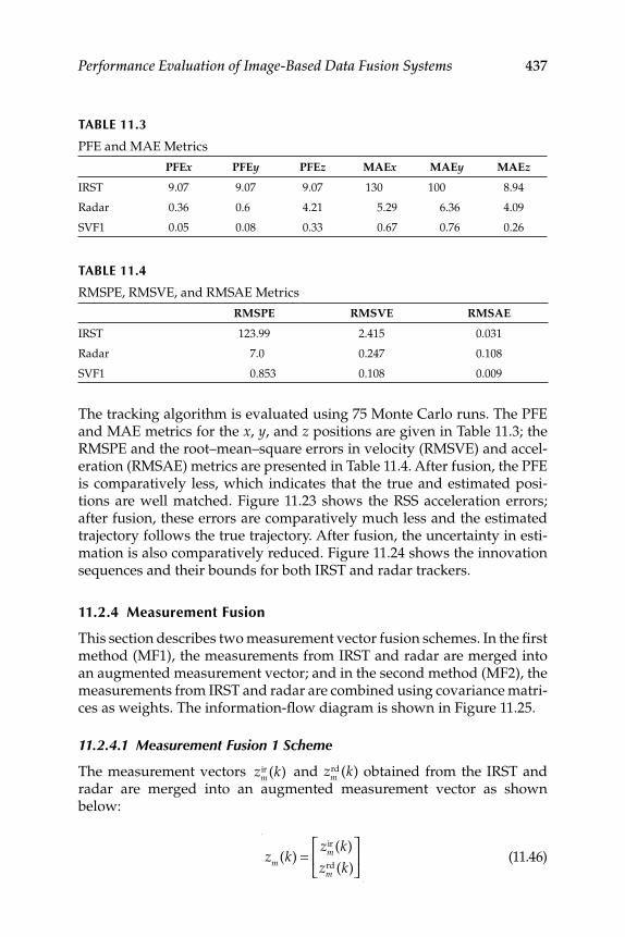
Performance Evaluation of Image-Based Data Fusion Systems 437

The tracking algorithm is evaluated using 75 Monte Carlo runs. The PFE and MAE metrics for the x , y , and z positions are given in Table 11.3; the RMSPE and the root–mean–square errors in velocity (RMSVE) and accel-eration (RMSAE) metrics are presented in Table 11.4. After fusion, the PFE is comparatively less, which indicates that the true and estimated posi-tions are well matched. Figure 11.23 shows the RSS acceleration errors; after fusion, these errors are comparatively much less and the estimated trajectory follows the true trajectory. After fusion, the uncertainty in esti-mation is also comparatively reduced. Figure 11.24 shows the innovation sequences and their bounds for both IRST and radar trackers.

11.2.4 Measurement Fusion

This section describes two measurement vector fusion schemes. In the fi rst method (MF1), the measurements from IRST and radar are merged into an augmented measurement vector; and in the second method (MF2), the measurements from IRST and radar are combined using covariance matri-ces as weights. The information-fl ow diagram is shown in Figure 11.25.

11.2.4.1 Measurement Fusion 1 Scheme

The measurement vectors zmir (k) and zm

rd (k) obtained from the IRST and radar are merged into an augmented measurement vector as shown below:

zm(k) =

zmir (k)

zmrd (k)

⎡

⎣⎢

⎤

⎦⎥

(11.46)

TABLE 11.3

PFE and MAE Metrics

PFEx PFEy PFEz MAEx MAEy MAEz

IRST 9.07 9.07 9.07 130 100 8.94

Radar 0.36 0.6 4.21 5.29 6.36 4.09

SVF1 0.05 0.08 0.33 0.67 0.76 0.26

TABLE 11.4

RMSPE, RMSVE, and RMSAE Metrics

RMSPE RMSVE RMSAE

IRST 123.99 2.415 0.031

Radar 7.0 0.247 0.108

SVF1 0.853 0.108 0.009

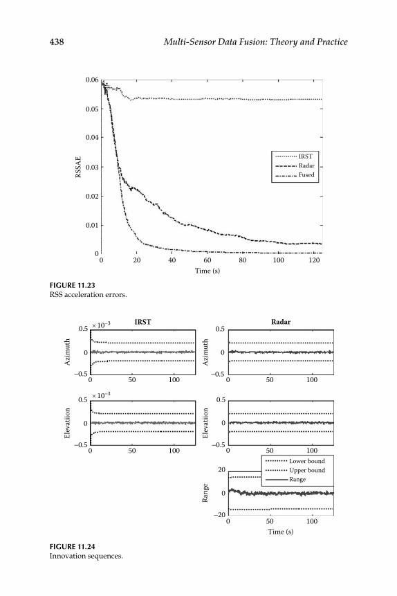
438 Multi-Sensor Data Fusion: Theory and Practice

FIGURE 11.23 RSS acceleration errors.

00 20 40 60

Time (s)80 100 120

0.01

0.02

0.03

RSSA

E

0.04

0.05

0.06

IRSTRadarFused

FIGURE 11.24 Innovation sequences.

IRST0.5 ´ 10−3

−0.5

0

0 50

Azim

uth

100

Radar0.5

−0.5

0

0 50

Azim

uth

100

0.5 ´ 10−3

−0.5

0

0 50

Elev

atiio

n

100

0.5

−0.5

0

0 50

Elev

atiio

n

100

20

−20

0

0 50

Rang

e

100Time (s)

Lower boundUpper boundRange

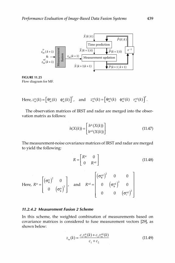
Performance Evaluation of Image-Based Data Fusion Systems 439

Here, zm

ir (k) = θmir (k) φm

ir (k)⎡⎣ ⎤⎦T, and

zm

rd (k) = θmrd (k) φm

rd (k) rmrd (k)⎡⎣ ⎤⎦

T.

The observation matrices of IRST and radar are merged into the obser-vation matrix as follows:

h(X(k)) =

hir (X(k))

hrd (X(k))

⎡

⎣⎢

⎤

⎦⎥

(11.47)

The measurement-noise covariance matrices of IRST and radar are merged to yield the following:

R =

Rir 0

0 Rrd

⎡

⎣⎢

⎤

⎦⎥

(11.48)

Here,

Rir =σθ

ir( )20

0 σφir( )2

⎡

⎣

⎢⎢⎢

⎤

⎦

⎥⎥⎥

, and

Rrd =

σθrd( )2

0 0

0 σφrd( )2

0

0 0 σrrd( )2

⎡

⎣

⎢⎢⎢⎢⎢

⎤

⎦

⎥⎥⎥⎥⎥

11.2.4.2 Measurement Fusion 2 Scheme

In this scheme, the weighted combination of measurements based on covariance matrices is considered to fuse measurement vectors [29], as shown below:

zm(k) =

c1zm

ir (k) + c2zm

rd (k)

c1

+ c2

(11.49)

FIGURE 11.25 Flow diagram for MF.

Time prediction

Measurement updation

z −1

Mea

sure

men

tfu

sion zm

(k + 1)zm ( k + 1)

zm (k + 1)

X (k + 1| k)~

X (k + 1|k + 1)ˆ

X (k | k )ˆ

P (k + 1| k)~

P (k + 1 | k + 1)ˆ

P (k | k )ˆ

&rd

ir

440 Multi-Sensor Data Fusion: Theory and Practice

where c1 and c2 are the weights. The weights in Equation 11.49 are com-puted from the measurement-noise covariance matrix as follows:

c1

= 1

Rirand c

2= 1

Rrd

zm(k) =

1

Rirzm

ir (k) + 1

Rrdzm

rd (k)

1

Rir+ 1

Rrd

(11.50)

The MF2 scheme is represented as follows:

zm(k) =

Rrdzmir (k) + Rirzm

rd (k)

Rir + Rrd (11.51)

or

zm(k) =Rrdzm

ir (k)

Rir + Rrd+

Rirzmrd (k)

Rir + Rrd+

Rirzmir (k)

Rir + Rrd−

Rirzmir (k)

Rir + Rrd

zm(k) = zmir (k) + Rir (Rir + Rrd )−1 zm

rd (k) − zmir (k)( )

(11.52)

The associated measurement-noise covariance matrix (R) of the fused measurement vector (Equation 11.52) is computed as follows:

1

R= 1

Rir+ 1

Rrd (11.53)

R = ((Rir )−1 + (Rrd )−1)−1

(11.54)

or

R = RirRrd

Rir + Rrd= RirRrd

Rir + Rrd− Rir + Rir

R = Rir + RirRrd − Rir (Rir + Rrd )

Rir + Rrd

R = Rir − Rir (Rir + Rrd )−1(Rir )T

(11.55)

11.2.5 Maneuvering Target Tracking

In tracking applications for a target moving with constant velocity (CV), the state model includes the fi rst derivative of the position, and for a

Performance Evaluation of Image-Based Data Fusion Systems 441

target moving with CA, the state model includes the second derivative of position. Models with second-order derivatives are preferred for track-ing maneuvering targets and are referred to as acceleration models. The IMMKF (see Section 3.5) is an adaptive state estimator that is based on the assumption that a fi nite number of models are required to characterize the motion of the target at all times.

11.2.5.1 Motion Models

The following two types of models in the Cartesian frame are considered for tracking a maneuvering targets:

1. The CV model (2-DOF kinematic model, with position and veloc-ity) with state-transition and process-noise gain matrices given as

F1

= FCV

=ΦV 0

3×30

3×3

03×3

ΦV 03×3

03×3

03×3

ΦV

⎡

⎣

⎢⎢⎢

⎤

⎦

⎥⎥⎥

G1= G

CV=

ςV 03×1

03×1

03×1

ςV 03×1

03×1

03×1

ςV

⎡

⎣

⎢⎢⎢

⎤

⎦

⎥⎥⎥

(11.56)

Here,

ΦV =1 T 0

0 1 0

0 0 0

⎡

⎣

⎢⎢⎢

⎤

⎦

⎥⎥⎥

ςV =T 2/2

T

0

⎡

⎣

⎢⎢⎢

⎤

⎦

⎥⎥⎥

03×3

=0 0 0

0 0 0

0 0 0

⎡

⎣

⎢⎢⎢

⎤

⎦

⎥⎥⎥

03×1

=0

0

0

⎡

⎣

⎢⎢⎢

⎤

⎦

⎥⎥⎥

The state vector is given as X = [x &x 0 y &y 0 z &z 0]T . The process-noise intensity (air turbulence, slow turns, and small linear acceleration) in each axis is generally assumed to be small

and equal in all three axes σx2 = σy

2 = σz2( ). Note that the accelera-

tion components in the model, although identically equal to zero, have been retained for dimensional compatibility with the third-order acceleration model.

2. The CA model (3-DOF kinematic model, with position, velocity, and acceleration) has the following state-transition and process-noise gain matrices:

F2

= FCA

=ΦA 0

3×30

3×3

03×3

ΦA 03×3

03×3

03×3

ΦA

⎡

⎣

⎢⎢⎢

⎤

⎦

⎥⎥⎥

G2= G

CA=

ςA 03×1

03×1

03×1

ςA 03×1

03×1

03×1

ςA

⎡

⎣

⎢⎢⎢

⎤

⎦

⎥⎥⎥

(11.57)

442 Multi-Sensor Data Fusion: Theory and Practice

Here,

ΦA =1 T T 2/2

0 1 T

0 0 1

⎡

⎣

⎢⎢⎢

⎤

⎦

⎥⎥⎥

ςA =T 3/6

T 2/2

T

⎡

⎣

⎢⎢⎢

⎤

⎦

⎥⎥⎥

03×3

=0 0 0

0 0 0

0 0 0

⎡

⎣

⎢⎢⎢

⎤

⎦

⎥⎥⎥

03×1

=0

0

0

⎡

⎣

⎢⎢⎢

⎤

⎦

⎥⎥⎥

The state vector in this model is X = [x &x &&x y &y &&y z &z &&z]T . A moderate value of the process-noise variance,

Q

CA (relatively

higher than QCV), will yield a nearly CA motion. The noise vari-

ances are assumed as σx2 = σy

2 = σz2( ).

11.2.5.2 Measurement Model

The measurement vector of the IRST is azimuth (θ) and elevation (φ), as represented in the expression

zm

ir (k) = θmir (k) φm

ir (k)⎡⎣ ⎤⎦T

(11.58)

The measurement vector of the radar is range (r), azimuth, and elevation and is given by the following equation:

zm

rd (k) = θmrd (k) φm

rd (k) rmrd (k)⎡⎣ ⎤⎦

T

(11.59)

These are related to the various states in a nonlinear fashion as follows:

x(k) = r(k)cosθ(k)cosφ(k)

y(k) = r(k)sin θ(k)cosφ(k)

z(k) = r(k)sin φ(k)

(11.60)

The measurement equation is given by

zm(k + 1) = h(X(k + 1) + v(k + 1))

(11.61)

11.2.5.3 Numerical Simulation

The target trajectory is simulated in Cartesian coordinates, with a sam-pling interval of 0.25 seconds using the CV model for the fi rst 50 seconds, followed by the CA model for 25 seconds, and then the CV model for 50 seconds. Acceleration magnitudes of 3 m/s2 and −3 m/s2 are injected at the time of maneuver along the x and y axes, respectively. The initial

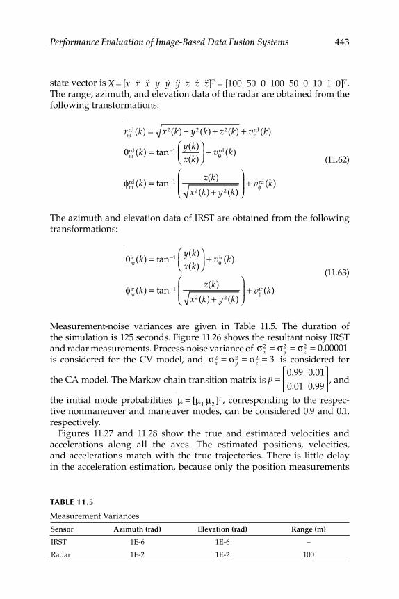
Performance Evaluation of Image-Based Data Fusion Systems 443

state vector is X = [x &x &&x y &y &&y z &z &&z]T = [100 50 0 100 50 0 10 1 0]T. The range, azimuth, and elevation data of the radar are obtained from the following transformations:

rmrd (k) = x2 (k) + y2 (k) + z2 (k) + vr

rd (k)

θmrd (k) = tan−1

y(k)

x(k)

⎛⎝⎜

⎞⎠⎟

+ vθrd (k)

φmrd (k) = tan−1

z(k)

x2 (k) + y2 (k)

⎛

⎝⎜

⎞

⎠⎟ + vφ

rd (k)

(11.62)

The azimuth and elevation data of IRST are obtained from the following transformations:

θmir (k) = tan−1

y(k)

x(k)

⎛⎝⎜

⎞⎠⎟

+ vθir (k)

φmir (k) = tan−1

z(k)

x2 (k) + y2 (k)

⎛

⎝⎜

⎞

⎠⎟ + vφ

ir (k)

(11.63)

Measurement-noise variances are given in Table 11.5. The duration of the simulation is 125 seconds. Figure 11.26 shows the resultant noisy IRST and radar measurements. Process-noise variance of σx

2 = σy2 = σz

2 = 0.00001 is considered for the CV model, and σx

2 = σy2 = σz

2 = 3 is considered for

the CA model. The Markov chain transition matrix is

p =

0.99 0.01

0.01 0.99

⎡

⎣⎢

⎤

⎦⎥ , and

the initial mode probabilities μ = [μ

1μ

2]T , corresponding to the respec-

tive nonmaneuver and maneuver modes, can be considered 0.9 and 0.1, respectively.

Figures 11.27 and 11.28 show the true and estimated velocities and accelerations along all the axes. The estimated positions, velocities, and accelerations match with the true trajectories. There is little delay in the acceleration estimation, because only the position measurements

TABLE 11.5

Measurement Variances

Sensor Azimuth (rad) Elevation (rad) Range (m)

IRST 1E-6 1E-6 –

Radar 1E-2 1E-2 100

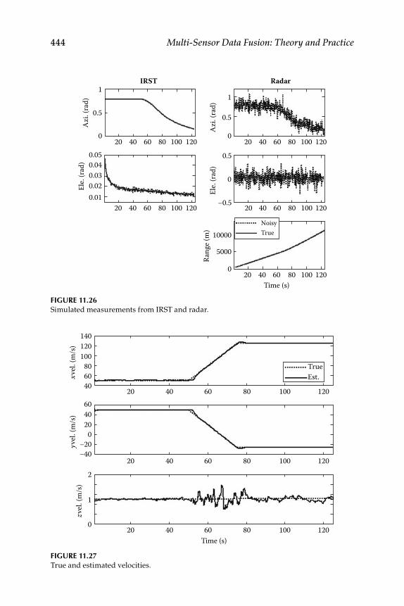
444 Multi-Sensor Data Fusion: Theory and Practice

FIGURE 11.26 Simulated measurements from IRST and radar.

IRST1

0.5

020 40 60 80 100 120

Azi. (

rad)

Radar

1

0.5

020 40 60 80 100 120

Azi. (

rad)

0.5

0

–0.5 20 40 60 80 100 120

20 40 60

10000

5000

0

Rang

e (m

)

Time (s)80 100 120

Ele.

(rad)

0.050.040.030.020.01

20 40 60 80 100 120

Ele.

(rad)

NoisyTrue

FIGURE 11.27 True and estimated velocities.

120100

xvel.

(m/s

)

806040

20 40 60 80 100 120

140

4020

yvel.

(m/s

)

0−20−40

20 40 60 80 100 120

60

zvel.

(m/s

)

1

020 40 60 80

Time (s)100 120

2

TrueEst.

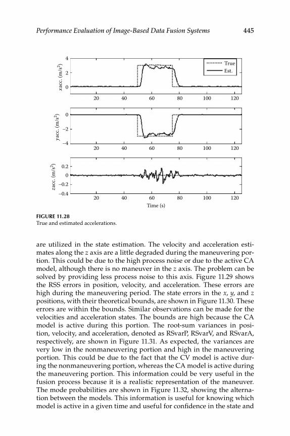
Performance Evaluation of Image-Based Data Fusion Systems 445

are utilized in the state estimation. The velocity and acceleration esti-mates along the z axis are a little degraded during the maneuvering por-tion. This could be due to the high process noise or due to the active CA model, although there is no maneuver in the z axis. The problem can be solved by providing less process noise to this axis. Figure 11.29 shows the RSS errors in position, velocity, and acceleration. These errors are high during the maneuvering period. The state errors in the x , y , and z positions, with their theoretical bounds, are shown in Figure 11.30. These errors are within the bounds. Similar observations can be made for the velocities and acceleration states. The bounds are high because the CA model is active during this portion. The root-sum variances in posi-tion, velocity, and acceleration, denoted as RSvarP, RSvarV, and RSvarA, respectively, are shown in Figure 11.31. As expected, the variances are very low in the nonmaneuvering portion and high in the maneuvering portion. This could be due to the fact that the CV model is active dur-ing the nonmaneuvering portion, whereas the CA model is active during the maneuvering portion. This information could be very useful in the fusion process because it is a realistic representation of the maneuver. The mode probabilities are shown in Figure 11.32, showing the alterna-tion between the models. This information is useful for knowing which model is active in a given time and useful for confi dence in the state and

FIGURE 11.28 True and estimated accelerations.

2

xacc

. (m

/s2 )

0

20 40 60 80 100 120

TrueEst.

4

0

yacc

. (m

/s2 )

-2

-4

-0.2-0.4

20 40 60 80 100 120

zacc

. (m

/s2 )

0

20 40 60 80Time (s)

100 120

0.2

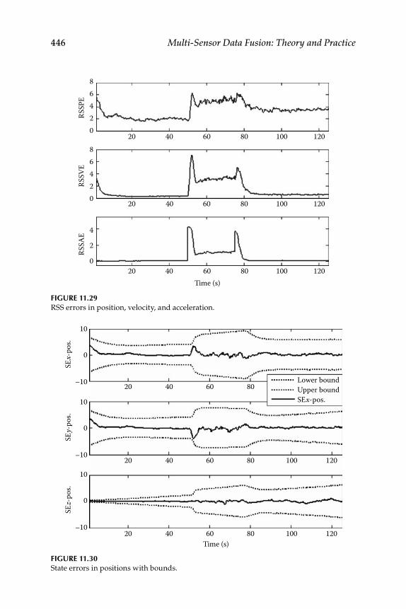
446 Multi-Sensor Data Fusion: Theory and Practice

FIGURE 11.30 State errors in positions with bounds.

0

–10 20 40 60 80Lower boundUpper boundSEx-pos.

20 40 60 80 100 120

20 40 60Time (s)

80 100 120

10

SEx-

pos.

0

–10

10

SEy-

pos.

0

–10

10

SEz-

pos.

FIGURE 11.29 RSS errors in position, velocity, and acceleration.

64

RSSP

E

20

20 40 60 80 100 120

20 40 60 80 100 120

20 40 60 80 100 120

8

64

RSSV

E

20

8

4

2

RSSA

E

0

Time (s)

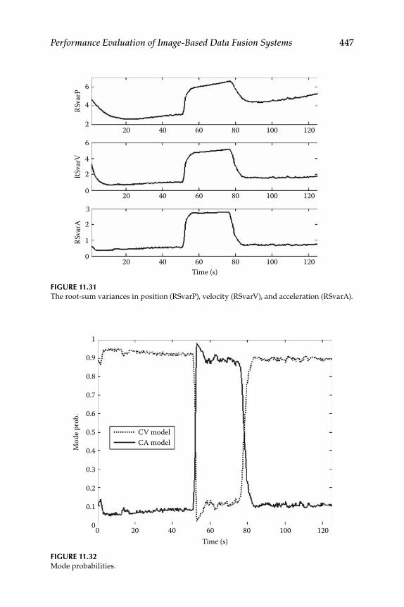
Performance Evaluation of Image-Based Data Fusion Systems 447

FIGURE 11.31 The root-sum variances in position (RSvarP), velocity (RSvarV), and acceleration (RSvarA).

6

4RSva

rP

220 40 60 80 100 120

20 40 60 80 100 120

20 40 60 80 100 120

4

RSva

rV

2

0

6

3

2

RSva

rA

1

0

Time (s)

FIGURE 11.32 Mode probabilities.

1

0.9

0.8

0.7

0.6

0.5

Mod

e pro

b.

0.4

0.3

0.2

0.1

00 20 40 60 80 100Time (s)

120

CV modelCA model

448 Multi-Sensor Data Fusion: Theory and Practice

state-error covariance matrix combination. The PFE metrics for positions, velocities, and accelerations along all three axes are depicted in Table 11.6a. The MAEs in positions, velocities, and accelerations of all the axes are shown in Table 11.6b. The RMSPE, RMSVE, and RMSAE are listed in Table 11.6c.

11.3 Target Tracking with Acoustic Sensor Arrays

and Imaging Sensor Data

This section discusses an approach to joint audio-video tracking based on acoustic sensor array (ASA) modeling, uniform linear array sensor data generation, and tracking a target in Cartesian coordinates. It also discusses the joint audio-video tracking of a target in 3-DOF Cartesian coordinates using decentralized KF.

11.3.1 Tracking with Multiple Acoustic Sensor Arrays

Target tracking using ASA is very useful in air-traffi c control, air defense, mobile-user location in cellular communications, military, underwater tracking, and acoustic source localization [30]. In ASA tracking, a sensor

TABLE 11.6A

PFE Metrics along the x, y, and z axes for the Positions, Velocities, and Accelerations

PFEx PFEy PFEz PFEx PFEy PFEz PFEx PFEy PFEz

0.049 0.113 2.175 1.43 3.56 78.11 46.947 46.987 61212.7

TABLE 11.6C

RMS Error Metrics for Position, Velocity, and Acceleration

RMSPE RMSVE RMSAE

2.339 1.185 0.536

TABLE 11.6B

MAE Metrics along the x, y, and z axes for the Positions, Velocities, and Accelerations

MAEx MAEy MAEz MAEx MAEy MAEz MAEx MAEy MAEz

1.1995 1.864 1.23 0.734 0.714 0.428 0.245 0.245 0.11

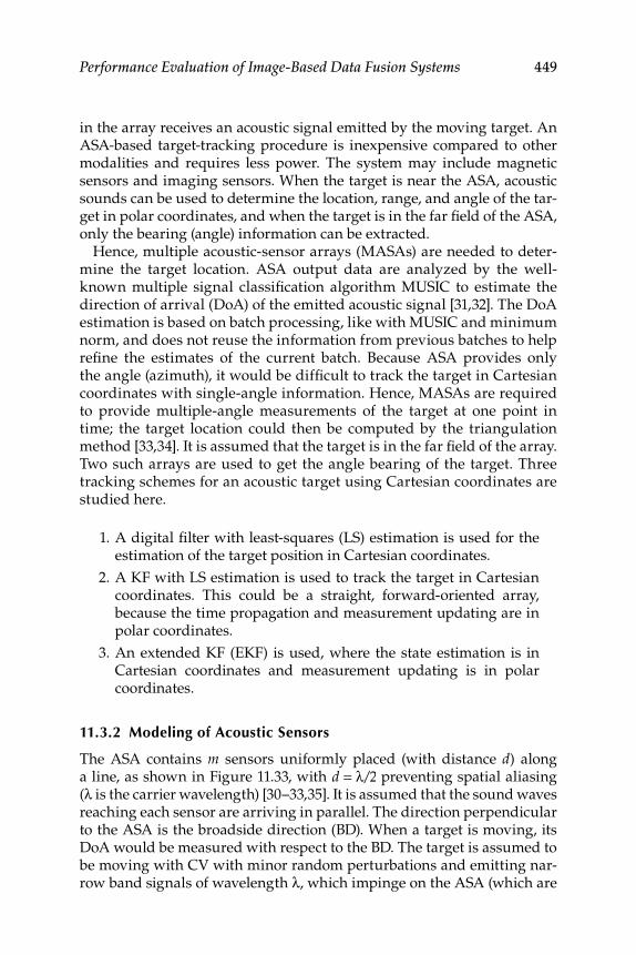
Performance Evaluation of Image-Based Data Fusion Systems 449

in the array receives an acoustic signal emitted by the moving target. An ASA-based target-tracking procedure is inexpensive compared to other modalities and requires less power. The system may include magnetic sensors and imaging sensors. When the target is near the ASA, acoustic sounds can be used to determine the location, range, and angle of the tar-get in polar coordinates, and when the target is in the far fi eld of the ASA, only the bearing (angle) information can be extracted.

Hence, multiple acoustic-sensor arrays (MASAs) are needed to deter-mine the target location. ASA output data are analyzed by the well-known multiple signal classifi cation algorithm MUSIC to estimate the direction of arrival (DoA) of the emitted acoustic signal [31,32]. The DoA estimation is based on batch processing, like with MUSIC and minimum norm, and does not reuse the information from previous batches to help refi ne the estimates of the current batch. Because ASA provides only the angle (azimuth), it would be diffi cult to track the target in Cartesian coordinates with single-angle information. Hence, MASAs are required to provide multiple-angle measurements of the target at one point in time; the target location could then be computed by the triangulation method [33,34]. It is assumed that the target is in the far fi eld of the array. Two such arrays are used to get the angle bearing of the target. Three tracking schemes for an acoustic target using Cartesian coordinates are studied here.

1. A digital fi lter with least-squares (LS) estimation is used for the estimation of the target position in Cartesian coordinates.

2. A KF with LS estimation is used to track the target in Cartesian coordinates. This could be a straight, forward-oriented array, because the time propagation and measurement updating are in polar coordinates.

3. An extended KF (EKF) is used, where the state estimation is in Cartesian coordinates and measurement updating is in polar coordinates.

11.3.2 Modeling of Acoustic Sensors

The ASA contains m sensors uniformly placed (with distance d ) along a line, as shown in Figure 11.33, with d = λ/2 preventing spatial aliasing (λ is the carrier wavelength) [30–33,35]. It is assumed that the sound waves reaching each sensor are arriving in parallel. The direction perpendicular to the ASA is the broadside direction (BD). When a target is moving, its DoA would be measured with respect to the BD. The target is assumed to be moving with CV with minor random perturbations and emitting nar-row band signals of wavelength λ, which impinge on the ASA (which are

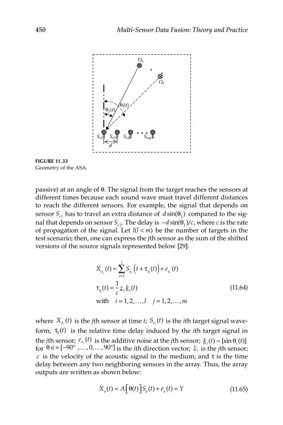
450 Multi-Sensor Data Fusion: Theory and Practice

passive) at an angle of θ. The signal from the target reaches the sensors at different times because each sound wave must travel different distances to reach the different sensors. For example, the signal that depends on

sensor Sr1 has to travel an extra distance of d sin(θ1) compared to the sig-

nal that depends on sensor Sr 2. The delay is −d sin(θ1)/c, where c is the rate

of propagation of the signal. Let l(l < m) be the number of targets in the test scenario; then, one can express the j th sensor as the sum of the shifted versions of the source signals represented below [29]:

Xaj(t) = Sai

t + τij (t)( ) + eaj(t)

i=1

l

∑

τij (t) = 1

cz j ki (t)

with i = 1, 2,…, l j = 1, 2,…, m

(11.64)

where Xaj

(t) is the j th sensor at time t; Sai

(t) is the i th target signal wave-

form; τij (t) is the relative time delay induced by the i th target signal in

the j th sensor; eaj

(t) is the additive noise at the j th sensor; k i (t) = [sin θi (t)]

for θ ∈= [−90° ,…, 0,…, 90°] is the i th direction vector; z j is the j th sensor;

c is the velocity of the acoustic signal in the medium; and τ is the time delay between any two neighboring sensors in the array. Thus, the array outputs are written as shown below:

Xa (t) = A θ(t)⎡⎣ ⎤⎦ Sa (t) + ea (t) = Y

(11.65)

FIGURE 11.33 Geometry of the ASA.

dSrmSr3Sr2Sr1

O1

Ol

θl(t)θ1(t)

Performance Evaluation of Image-Based Data Fusion Systems 451

where Xa(t) = Xa1(t) L Xam

(t)T is an m vector of the complex envelopes of

the sensor outputs; Sa (t)= Sa1(t) L Sal

(t)⎡⎣

⎤⎦

T is an l vector of the complex

envelopes of the target signals; ea(t) = ea1(t) L e am

(t)⎡⎣

⎤⎦

T denotes an m vector

of the complex envelopes of the additive measurement noises (with the

usual assumptions); A θ(t)⎡⎣ ⎤⎦ = a(θ1) L a(θ l)⎡⎣ ⎤⎦ is the m × l Vandermode

matrix (steering matrix); a(θi ) = 1e− j2π

dλ

sin θi L e− j(m−1)2π

dλ

sin θi⎡

⎣⎢

⎤

⎦⎥

T

is the steer-

ing vector for the i th source/target signal with unit-magnitude elements;

and θ(t) = θ

1(t) L θl (t)⎡⎣ ⎤⎦

T is the unknown DoA vector (of the l targets

at time t) to be estimated. The term θ(t) is a slowly varying function. Because the change in θ(t) is either zero or negligible in each interval

of nT, (n + 1)T⎡⎣ ⎤⎦ , n = 0,1, 2, ..., the term θ(t) can be further modifi ed as

θ(t) ≈ θ(nT) for t ∈[nT, (n + 1)T], n = 0,1, 2, ..., (11.66)

In an interval N, snapshots of the sensor data are available for processing. Based on the assumptions made in Equation 11.66, these N snapshots of sensor data are expressed as shown below:

Xa (k) ≈ A[θ(n)]Sa (k) + ea (k), k = n, n + 1, n + 2,..., n + N − 1 (11.67)

Equation 11.67 is the discrete form of Equation 11.65 with a sampling

interval of T/N.

11.3.3 DoA Estimation

The MUSIC algorithm is one of the most popular subspace methods used in spectral estimation [31]. Let us consider the following ASA output data from Equation 11.65:

Y = ASa + ea (11.68)

If the signals from different targets/sources are uncorrelated, the correla-tion matrix of Y is written as

Ra = E{YYT } = E ASaSaT AT{ } + E eaea

T{ }Ra = ARs AT + σ2I = Z + σ2I

(11.69)

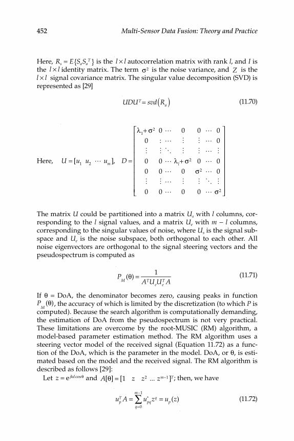
452 Multi-Sensor Data Fusion: Theory and Practice

Here, Rs = E SaSaT{ } is the l × l autocorrelation matrix with rank l, and I is

the l × l identity matrix. The term σ2 is the noise variance, and Z is the l × l signal covariance matrix. The singular value decomposition (SVD) is represented as [29]

UDUT = svd Ra( )

(11.70)

Here,

U = [u1

u2

L um ], D =

λ1+ σ2 0 L 0 0 L 0

0 : L M M L 0

M M O M M L M0 0 L λl+ σ2 0 L 0

0 0 L 0 σ2 L 0

M M L M M O M0 0 L 0 0 L σ2

⎡

⎣

⎢⎢⎢⎢⎢⎢⎢⎢⎢

⎤

⎦

⎥⎥⎥⎥⎥⎥⎥⎥⎥

The matrix U could be partitioned into a matrix Us with l columns, cor-responding to the l signal values, and a matrix Ue with m − l columns, corresponding to the singular values of noise, where Us is the signal sub-space and Ue is the noise subspace, both orthogonal to each other. All noise eigenvectors are orthogonal to the signal steering vectors and the pseudospectrum is computed as

P

M(θ) = 1

ATUeUeT A

(11.71)

If θ = DoA, the denominator becomes zero, causing peaks in function P

M(θ), the accuracy of which is limited by the discretization (to which P is

computed). Because the search algorithm is computationally demanding, the estimation of DoA from the pseudospectrum is not very practical. These limitations are overcome by the root-MUSIC (RM) algorithm, a model-based parameter estimation method. The RM algorithm uses a steering vector model of the received signal (Equation 11.72) as a func-tion of the DoA, which is the parameter in the model. DoA, or θ, is esti-mated based on the model and the received signal. The RM algorithm is described as follows [29]:

Let z = e jkd cosθ and A[θ] = [1 z z2 ... zm−1]T; then, we have

up

T A = upq*

q=0

m−1

∑ zq = up (z) (11.72)

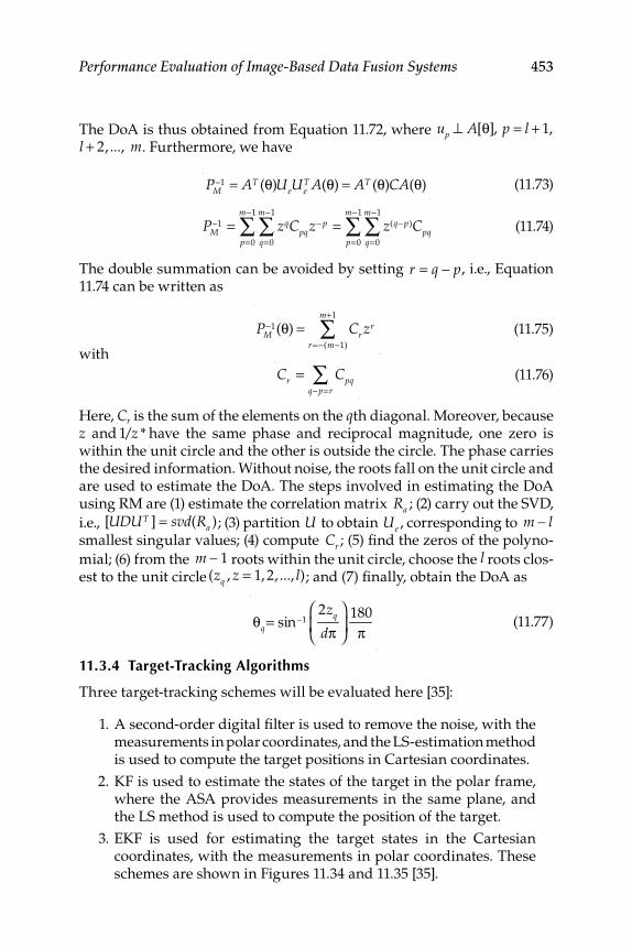
Performance Evaluation of Image-Based Data Fusion Systems 453

The DoA is thus obtained from Equation 11.72, where up ⊥ A[θ], p = l + 1,

l + 2,..., m. Furthermore, we have

PM

−1 = AT (θ)UeUeT A(θ) = AT (θ)CA(θ) (11.73)

PM

−1 = zqCpqz− p

q=0

m−1

∑p=0

m−1

∑ = z(q−p)Cpqq=0

m−1

∑p=0

m−1

∑ (11.74)

The double summation can be avoided by setting r = q − p, i.e., Equation 11.74 can be written as

PM

−1(θ) = Cr zr

r=−(m−1)

m+1

∑ (11.75)

with

Cr = Cpq

q−p=r∑ (11.76)

Here, Cr is the sum of the elements on the q th diagonal. Moreover, because z and

1/z * have the same phase and reciprocal magnitude, one zero is within the unit circle and the other is outside the circle. The phase carries the desired information. Without noise, the roots fall on the unit circle and are used to estimate the DoA. The steps involved in estimating the DoA using RM are (1) estimate the correlation matrix Ra ; (2) carry out the SVD,

i.e., [UDUT ] = svd(Ra ); (3) partition U to obtain Ue , corresponding to m − l

smallest singular values; (4) compute Cr ; (5) fi nd the zeros of the polyno-

mial; (6) from the m − 1 roots within the unit circle, choose the l roots clos-est to the unit circle (zq , z = 1, 2, ..., l); and (7) fi nally, obtain the DoA as

θq= sin−12zq

dπ⎛

⎝⎜

⎞

⎠⎟

180

π (11.77)

11.3.4 Target-Tracking Algorithms

Three target-tracking schemes will be evaluated here [35]:

1. A second-order digital fi lter is used to remove the noise, with the measurements in polar coordinates, and the LS-estimation method is used to compute the target positions in Cartesian coordinates.

2. KF is used to estimate the states of the target in the polar frame, where the ASA provides measurements in the same plane, and the LS method is used to compute the position of the target.

3. EKF is used for estimating the target states in the Cartesian coordinates, with the measurements in polar coordinates. These schemes are shown in Figures 11.34 and 11.35 [35].

454 Multi-Sensor Data Fusion: Theory and Practice

FIGURE 11.34 Target tracker for schemes 1 and 2.

ASA1 ASA2

y

x

y

x

Target

Estimationof DoA

Estimationof DoA

DF or KF DF or KF

Least squares method

Position of target/trajectory estimated

θ1 θ2

θ1θ2

FIGURE 11.35 Target tracker for scheme 3.

ASA1 ASA2

y

x

y

x

Target

Estimationof DoA

Estimationof DoA

EKF

Position of target/trajectory estimated

θ1θ2

θ1 θ2

Performance Evaluation of Image-Based Data Fusion Systems 455

11.3.4.1 Digital Filter

The ASA provides noisy measurements in polar coordinates. A second- order low-pass digital Butterworth fi lter with a normalized cutoff frequency of 0.5 is used to remove the noise. The transfer function, H(z), of the fi lter is

H(z) =

b0

+ b1z−1 + b

2z−2

1 + a1z−1 + a

2z−2

(11.78)

Here, n is the order of the fi lter; b 0 , bi, and b 2 are numerator coeffi cients, and ai and a 2 are the denominator coeffi cients.

11.3.4.2 Triangulation

For scheme 1, the measurements are in polar coordinates. To obtain the target position in Cartesian coordinates, LS estimation is used [33]. If the true target positions in Cartesian coordinates are (x

tr, y

tr), the locations of

the two sensors Sr1 and Sr 2 are (Sr1x , Sr1y ) and (Sr 2x, Sr 2y ), and the target is at θ

1and θ

2with respect to Sr1

and Sr 2, respectively, then

tan(θ

1) =

ytr

− Sr1y

xtr

− Sr1x

and tan(θ2) =

ytr

− Sr 2y

xtr

− Sr 2x

(11.79)

After rearrangement, we obtain

Sr1y − Sr1x tan(θ1)

Sr 2y − Sr 2x tan(θ2)

⎡

⎣⎢⎢

⎤

⎦⎥⎥

=− tan(θ

1) 1

− tan(θ2) 1

⎡

⎣⎢

⎤

⎦⎥

xtr

ytr

⎡

⎣⎢

⎤

⎦⎥

(11.80)

which is represented as

f = Bg (11.81)

Here, B and f are known and g is unknown; then, the target position g

is computed from g = B−1 f .

11.3.4.3 Results and Discussion

For the performance evaluation of the DoA algorithm, the parameters given in Table 11.7 and 50 Monte Carlo simulations are used to obtain the results. Figure 11.36a is obtained by varying the variance level from 0 to 0.1 and keeping the other parameters constant, as shown in Table 11.7. The AE in DoA increases with an increase in the noise level. Keeping the other parameters constant, the effect of the snapshots is shown in Figure 11.36b. The AE decreases with an increase in the number of snapshots.

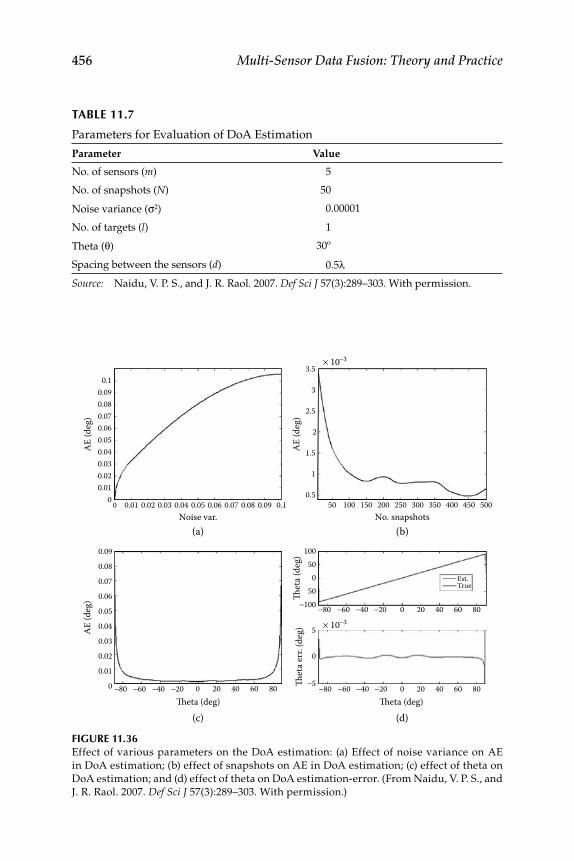
456 Multi-Sensor Data Fusion: Theory and Practice

FIGURE 11.36 Effect of various parameters on the DoA estimation: (a) Effect of noise variance on AE

in DoA estimation; (b) effect of snapshots on AE in DoA estimation; (c) effect of theta on

DoA estimation; and (d) effect of theta on DoA estimation-error. (From Naidu, V. P. S., and

J. R. Raol. 2007. Def Sci J 57(3):289–303. With permission.)

× 10−3

× 10−3

AE (d

eg)

AE (d

eg)

Thet

a (de

g)Th

eta e

rr. (d

eg)

Theta (deg)Theta (deg)

AE (d

eg)

0 0 0.01 0.02 0.03 0.04 0.05Noise var.

(a) (b)

(c) (d)

0.06 0.07 0.08 0.09 0.1

0.010.020.030.040.050.060.070.080.09

3.5

3

2.5

2

1.5

1

0.5

10050

0

0

5

−5

50−100

50 100 150 200 250No. snapshots

300 350 400 450 500

0 −80 −60 −40 −20 0 20 40 60 80

−80 −60 −40 −20 0 20 40 60 80

−80 −60 −40 −20 0 20 40 60 80

0.01

0.02

0.03

0.04

0.05

0.06

0.07

0.08

0.09

0.1

Est.True

TABLE 11.7

Parameters for Evaluation of DoA Estimation

Parameter Value

No. of sensors (m) 5

No. of snapshots (N) 50

Noise variance (σ2) 0.00001

No. of targets (l) 1

Theta (θ) 30º

Spacing between the sensors (d) 0.5λ

Source: Naidu, V. P. S., and J. R. Raol. 2007. Def Sci J 57(3):289–303. With permission.

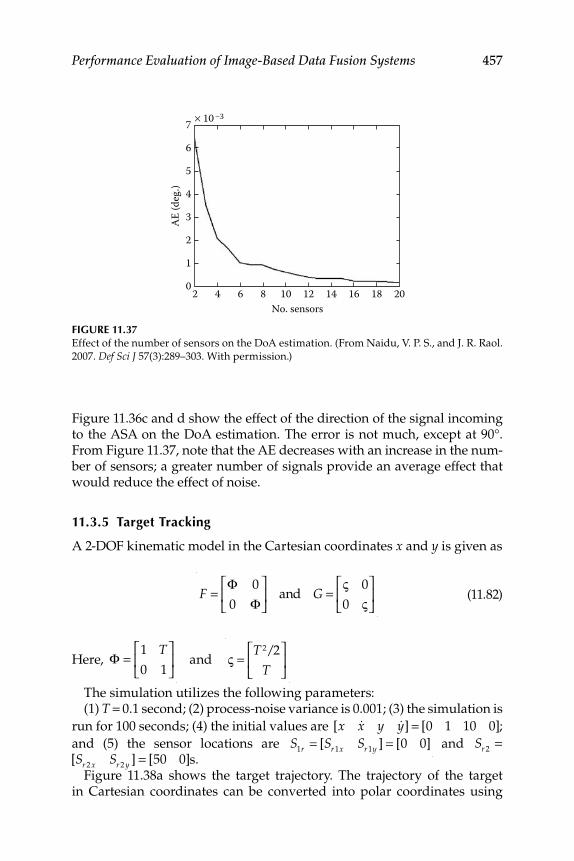
Performance Evaluation of Image-Based Data Fusion Systems 457

Figure 11.36c and d show the effect of the direction of the signal incoming to the ASA on the DoA estimation. The error is not much, except at 90°. From Figure 11.37, note that the AE decreases with an increase in the num-ber of sensors; a greater number of signals provide an average effect that would reduce the effect of noise.

11.3.5 Target Tracking

A 2-DOF kinematic model in the Cartesian coordinates x and y is given as

F =

Φ 0

0 Φ⎡

⎣⎢

⎤

⎦⎥ and G =

ς 0

0 ς⎡

⎣⎢

⎤

⎦⎥ (11.82)

Here,

Φ =

1 T

0 1

⎡

⎣⎢

⎤

⎦⎥ and

ς =

T 2/2

T

⎡

⎣⎢

⎤

⎦⎥

The simulation utilizes the following parameters: (1) T = 0.1 second; (2) process-noise variance is 0.001; (3) the simulation is

run for 100 seconds; (4) the initial values are [x &x y &y] = [0 1 10 0];

and (5) the sensor locations are S

1r = [Sr1x Sr1y ] = [0 0] and Sr 2=

[Sr 2x Sr 2y ] = [50 0]s. Figure 11.38a shows the target trajectory. The trajectory of the target

in Cartesian coordinates can be converted into polar coordinates using

FIGURE 11.37 Effect of the number of sensors on the DoA estimation. (From Naidu, V. P. S., and J. R. Raol.

2007. Def Sci J 57(3):289–303. With permission.)

7 × 10 −3

6

5

4

3AE (d

eg.)

2

1

02 4 6 8 10 12No. sensors

14 16 18 20

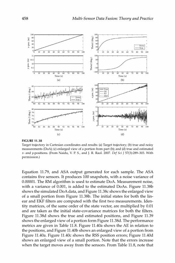
458 Multi-Sensor Data Fusion: Theory and Practice

Equation 11.79, and ASA output generated for each sample. The ASA contains fi ve sensors. It produces 100 snapshots, with a noise variance of 0.00001. The RM algorithm is used to estimate DoA. Measurement noise, with a variance of 0.001, is added to the estimated DoAs. Figure 11.38b shows the simulated DoA data, and Figure 11.38c shows the enlarged view of a small portion from Figure 11.38b. The initial states for both the lin-ear and EKF fi lters are computed with the fi rst two measurements. Iden-tity matrices, of the same order of the state vector, are multiplied by 0.01 and are taken as the initial state-covariance matrices for both the fi lters. Figure 11.38d shows the true and estimated positions, and Figure 11.39 shows the enlarged view of a portion form Figure 11.38d. The performance metrics are given in Table 11.8. Figure 11.40a shows the AE in relation to the positions, and Figure 11.40b shows an enlarged view of a portion from Figure 11.40a. Figure 11.40c shows the RSS position errors; Figure 11.40d shows an enlarged view of a small portion. Note that the errors increase when the target moves away from the sensors. From Table 11.8, note that

FIGURE 11.38 Target trajectory in Cartesian coordinates and results: (a) Target trajectory; (b) true and noisy

measurements (DoA); (c) enlarged view of a portion from part (b); and (d) true and estimated

x- and y-positions. (From Naidu, V. P. S., and J. R. Raol. 2007. Def Sci J 57(3):289–303. With

permission.)

00204060

x-po

s. (m

) 80100

10 20 30 40 50 60 70 80 90 100

02040

TrueDFKFEKF

60x.p

os. (

m) 80

100

10 20 30 40 50 60 70 80 90 100

Time (s)

Time (s)(a)

(c) (d)

(b)

9.5

10

10.5

y-po

s. (m

)

11

09 10 20 30 40 50Time (s)

60 70 80 90 100

83

84

85

Thet

a 1 (d

eg.)

8082 82 84 86 88 90 92 94 96 98 100

00

204060

Thet

a1 (d

eg.) 80

100

10 20 30 40 50 60 70 80 90

NoisyTrue

NoisyTrue

7274767880

Thet

a 2 (d

eg.)

8070 82 84 86 88 90 92 94 96 98 100

100

0-100

-50

0

50

Thet

a2 (d

eg.)

100

10 20 30 40 50 60 70 80 90 100

Time (s)8

9

10

11

y.pos

. (m

)

12

10 20 30 40 50 60 70 80 90 100

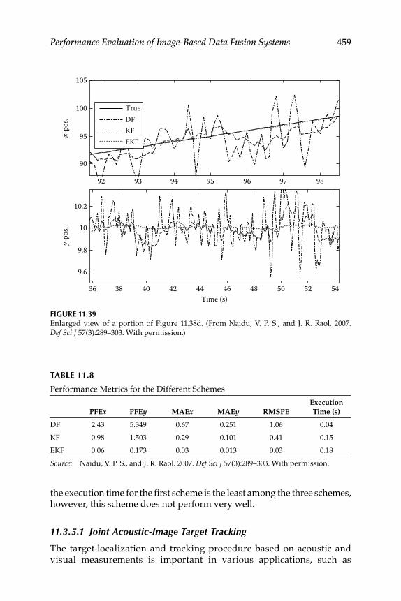
Performance Evaluation of Image-Based Data Fusion Systems 459

the execution time for the fi rst scheme is the least among the three schemes, however, this scheme does not perform very well.

11.3.5.1 Joint Acoustic-Image Target Tracking

The target-localization and tracking procedure based on acoustic and visual measurements is important in various applications, such as

FIGURE 11.39 Enlarged view of a portion of Figure 11.38d. (From Naidu, V. P. S., and J. R. Raol. 2007.

Def Sci J 57(3):289–303. With permission.)

92 93 94 95 96 97 98

90

95

100

105

x-po

s.

36 38 40 42 44 46 48 50 52 54

9.6

9.8

10

10.2

Time (s)

y-po

s.

TrueDFKFEKF

TABLE 11.8

Performance Metrics for the Different Schemes

PFEx PFEy MAEx MAEy RMSPE

Execution

Time (s)

DF 2.43 5.349 0.67 0.251 1.06 0.04

KF 0.98 1.503 0.29 0.101 0.41 0.15

EKF 0.06 0.173 0.03 0.013 0.03 0.18

Source: Naidu, V. P. S., and J. R. Raol. 2007. Def Sci J 57(3):289–303. With permission.

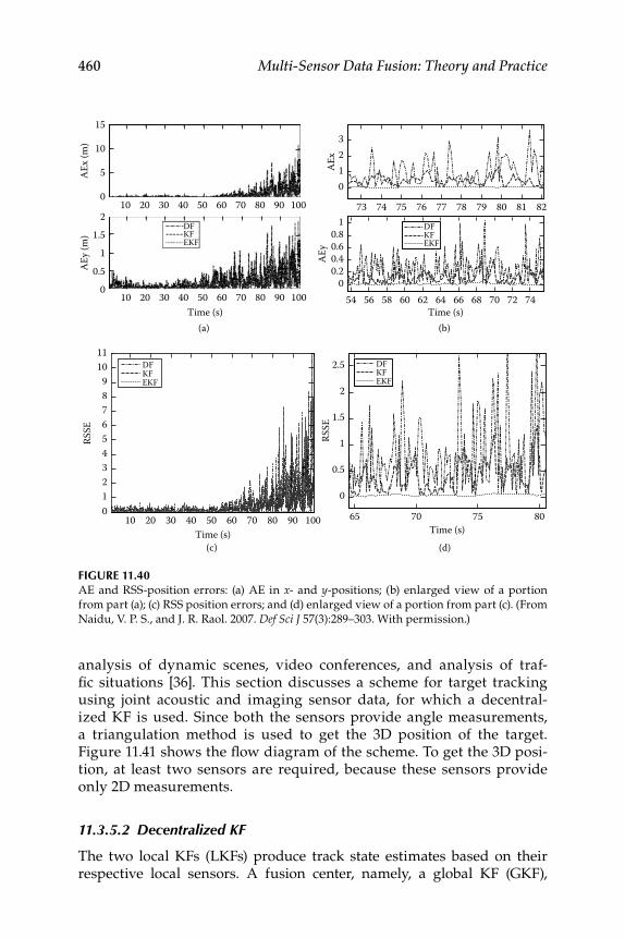
460 Multi-Sensor Data Fusion: Theory and Practice

analysis of dynamic scenes, video conferences, and analysis of traf-fi c situations [36]. This section discusses a scheme for target tracking using joint acoustic and imaging sensor data, for which a decentral-ized KF is used. Since both the sensors provide angle measurements, a triangulation method is used to get the 3D position of the target. Figure 11.41 shows the fl ow diagram of the scheme. To get the 3D posi-tion, at least two sensors are required, because these sensors provide only 2D measurements.

11.3.5.2 Decentralized KF

The two local KFs (LKFs) produce track state estimates based on their respective local sensors. A fusion center, namely, a global KF (GKF),

FIGURE 11.40 AE and RSS-position errors: (a) AE in x- and y-positions; (b) enlarged view of a portion

from part (a); (c) RSS position errors; and (d) enlarged view of a portion from part (c). (From

Naidu, V. P. S., and J. R. Raol. 2007. Def Sci J 57(3):289–303. With permission.)

73 74 75 76 77 78 79 80 81 82

0123

AEx

54Time (s)

56 58 60 62 64 66 68 70 72 740

0.20.40.60.8

1

AEy

DFKFEKF

(b)

Time (s)10 20 30 40 50 60 70 80 90 100

0123456789

1011

RSSE

DFKFEKF

(c) Time (s)

65 70 75 80

0

0.5

1

1.5

2

2.5

RSSE

DFKFEKF

(d)

10

21.5

AEy (

m)

10.5

020 30 40 50

DFKFEKF

Time (s)60 70 80 90 100

10

15

10

AEx (

m)

5

020 30 40 50 60 70 80 90 100

(a)

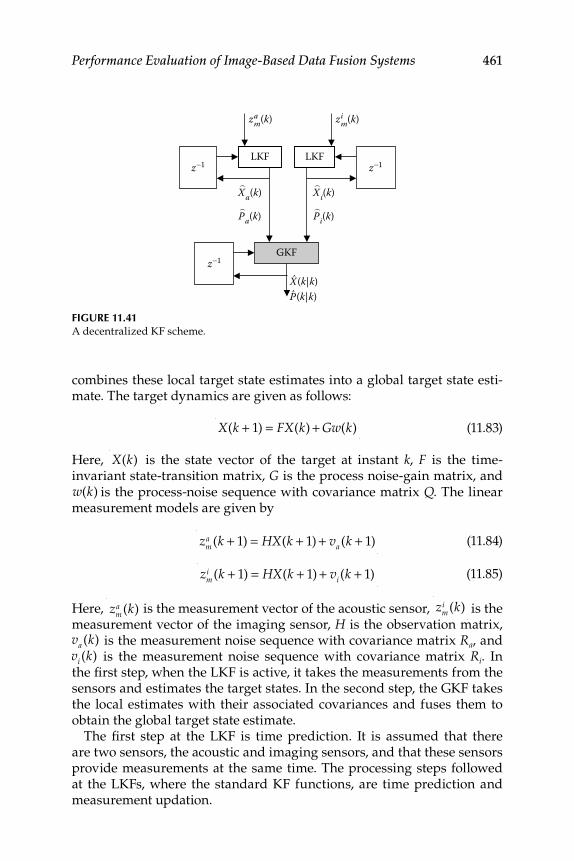
Performance Evaluation of Image-Based Data Fusion Systems 461

combines these local target state estimates into a global target state esti-mate. The target dynamics are given as follows:

X(k + 1) = FX(k) + Gw(k) (11.83)

Here, X(k) is the state vector of the target at instant k, F is the time-

invariant state-transition matrix, G is the process noise-gain matrix, and w(k) is the process-noise sequence with covariance matrix Q. The linear measurement models are given by

zm

a (k + 1) = HX(k + 1) + va (k + 1) (11.84)

zm

i (k + 1) = HX(k + 1) + vi (k + 1) (11.85)

Here, zma (k) is the measurement vector of the acoustic sensor,

zm

i (k) is the measurement vector of the imaging sensor, H is the observation matrix, va (k) is the measurement noise sequence with covariance matrix Ra, and vi (k) is the measurement noise sequence with covariance matrix Ri. In the fi rst step, when the LKF is active, it takes the measurements from the sensors and estimates the target states. In the second step, the GKF takes the local estimates with their associated covariances and fuses them to obtain the global target state estimate.

The fi rst step at the LKF is time prediction. It is assumed that there are two sensors, the acoustic and imaging sensors, and that these sensors provide measurements at the same time. The processing steps followed at the LKFs, where the standard KF functions, are time prediction and measurement updation.

FIGURE 11.41 A decentralized KF scheme.

LKF

X a(k)

LKF

GKF

z am(k) z

im(k)

z -1z

-1

z -1

P a(k)

X i(k)

P i(k)

X(k|k)P(k|k)

462 Multi-Sensor Data Fusion: Theory and Practice

Time prediction is carried out as follows:

(a) At the acoustic sensor:

%Xa (k|k − 1) = FXa (k − 1|k − 1) (11.86)

%Pa (k|k − 1) = FPa (k − 1|k − 1)FT + GQGT (11.87)

(b) At the imaging sensor:

%Xi (k|k − 1) = FXi (k − 1|k − 1) (11.88)

%Pi (k|k − 1) = FPi (k − 1|k − 1)FT + GQGT (11.89)

Measurement update is carried out as follows:

(a) At the acoustic sensor:

ϑ = zma (k) − H %Xa (k|k − 1) (11.90)

S = H %Pa (k|k − 1)HT + Ra (11.91)

K = %Pa (k|k − 1)HTS−1 (11.92)

Xa (k|k) = %Xa (k|k − 1) + Kϑ (11.93)

Pa (k|k) = [I − KH] %Pa (k|k − 1) (11.94)

)Xa (k) = Pa

−1(k|k)Xa (k|k) − %Pa−1(k|k − 1) %Xa (k|k − 1) (11.95)

)Pa (k) =

)Pa

−1(k|k) −)Pa

−1(k|k − 1) (11.96)

(b) At the imaging sensor:

ϑ = zmi (k) − H %Xi (k|k − 1) (11.97)

S = H %Pi (k|k − 1)HT + Ri (11.98)

K = %Pi (k|k − 1)HTS−1 (11.99)

Xi (k|k) = %Xi (k|k − 1) + Kϑ (11.100)

Pi (k|k) = [I − KH] %Pi (k|k − 1) (11.101)

Performance Evaluation of Image-Based Data Fusion Systems 463

)Xi (k) = Pi

−1(k|k)Xi (k|k) − %Pi−1(k|k − 1) %Xi (k|k − 1) (11.102)

)Pi (k) =

)Pi

−1(k|k) −)Pi

−1(k|k − 1) (11.103)

The processing steps followed at the fusion center, where the GKF is func-tional, are as follows:

(a) Time prediction:

%X(k|k − 1) = FX(k − 1|k − 1) (11.104)

%P(k|k − 1) = FP(k − 1|k − 1)FT + GQGT (11.105)

(b) Estimate correction:

P−1(k|k) = %P−1(k|k − 1) +

)Pa (k) +

)Pi (k) (11.106)

X(k|k) = P(k|k) %P−1(k|k − 1) %X(k|k − 1) +

)Xa (k) +

)Xi (k)⎡⎣ ⎤⎦ (11.107)

11.3.5.3 3D Target Tracking

Because the ASA provides only angle measurements, triangulation is used to obtain the target’s 3D position. The two sensors are placed at two different locations. Each set contains both acoustic and imaging sensors. Figure 11.42 shows the general scheme. The estimates from the two fusion centers are used to determine the 3D target position using triangulation. Let the target state estimate from the fi rst and the second fusion centers be

X

1(k|k) = θ

1&θ

1&&θ

1φ

1&φ

1&&φ

1⎡⎣ ⎤⎦

T (11.108)

X

2(k|k) = θ

2&θ

2&&θ

2φ

2&φ

2&&φ

2⎡⎣ ⎤⎦

T (11.109)

Similarly, let the locations of the two sensor sets, Sr1 and Sr1, be (Sr1x, Sr1y, Sr1z) and (Sr2x, Sr2y, Sr2z), respectively. Let the target be at an angle of (θ

1, φ

1)

and (θ2, φ

2) with respect to Sr1 and Sr2. Let the target position in Cartesian

coordinates be (xtr, ytr, ztr). Then

tan(θ

1) =

ytr

− Sr1y

xtr

− Sr1x

(11.110)

tan(θ

2) =

ytr

− Sr 2y

xtr

− Sr 2x

(11.111)

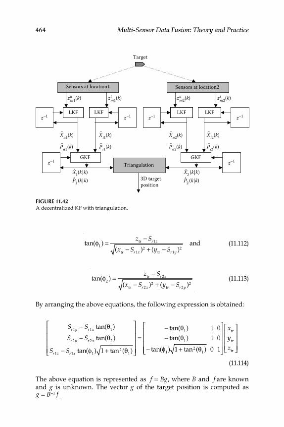
464 Multi-Sensor Data Fusion: Theory and Practice

tan(φ1) =

ztr

− Sr1z

(xtr

− Sr1x )2 + (ytr

− Sr1y )2and (11.112)

tan(φ2) =

ztr

− Sr 2z

(xtr

− Sr 2x )2 + (ytr

− Sr 2y )2 (11.113)

By arranging the above equations, the following expression is obtained:

Sr1y − Sr1x tan(θ1)

Sr 2y − Sr 2x tan(θ2)

Sr1z − Sr1x tan(φ1) 1 + tan2 (θ

1)

⎡

⎣

⎢⎢⎢⎢

⎤

⎦

⎥⎥⎥⎥

=− tan(θ

1) 1 0

− tan(θ1) 1 0

− tan(φ1) 1 + tan2 (θ

1) 0 1

⎡

⎣

⎢⎢⎢⎢

⎤

⎦

⎥⎥⎥⎥

xtr

ytr

ztr

⎡

⎣

⎢⎢⎢

⎤

⎦

⎥⎥⎥

(11.114)

The above equation is represented as f = Bg, where B and f are known and g is unknown. The vector g of the target position is computed as g = B−1 f .

FIGURE 11.42 A decentralized KF with triangulation.

3D targetposition

z am2(k)

LKF LKF

GKF

z im1(k)

Triangulation

LKF LKF

GKF

Sensors at location1 Sensors at location2

Target

z am1(k) z

im2(k)

z -1 z

-1 z -1 z

-1

z -1 z

-1

X a1(k)

P a1(k)

X a2(k)

P a2(k)

X i2(k)

P i2(k)

X i1(k)

P i1(k)

X1(k|k)P1

(k|k)X2

(k|k)P2

(k|k)

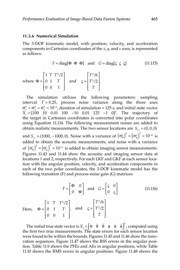
Performance Evaluation of Image-Based Data Fusion Systems 465

11.3.6 Numerical Simulation

The 3-DOF kinematic model, with position, velocity, and acceleration components in Cartesian coordinates of the x , y , and z axes, is represented as follows:

F = diag[Φ Φ Φ] and G = diag[ς ς ς] (11.115)

where Φ =1 T T 2/2

0 1 T

0 0 1

⎡

⎣

⎢⎢⎢

⎤

⎦

⎥⎥⎥ and

ς =T 3/6

T 2/2

T

⎡

⎣

⎢⎢⎢

⎤

⎦

⎥⎥⎥.

The simulation utilizes the following parameters: sampling interval T = 0.25, process noise variance along the three axes

σx2 = σy

2 = σz2 = 10−6, duration of simulation = 125 s, and initial state vector

Xi = [100 10 0.01 100 −10 0.01 125 −1 0]T. The trajectory of the target in Cartesian coordinates is converted into polar coordinates using Equation 11.114. The following measurement noises are added to

obtain realistic measurements. The two sensor locations are Sr1

= (0, 0, 0)

and Sr1= (1000, −1000, 0). Noise with a variance of

σθ

a( )2= σφ

a( )2

= 10−4 is

added to obtain the acoustic measurements, and noise with a variance

of σθi( )2

= σφi( )2

= 10−6 is added to obtain imaging sensor measurements.

Figures 11.43 and 11.44 show the acoustic and imaging sensor data at locations 1 and 2, respectively. For each LKF and GKF at each sensor loca-tion with the angular position, velocity, and acceleration components in each of the two polar coordinates, the 3-DOF kinematic model has the following transition (F) and process-noise gain (G) matrices:

F =

Φ 0

0 Φ⎡

⎣⎢

⎤

⎦⎥ and G =

ς 0

0 ς⎡

⎣⎢

⎤

⎦⎥ (11.116)

Here, Φ =1 T T 2/2

0 1 T

0 0 1

⎡

⎣

⎢⎢⎢

⎤

⎦

⎥⎥⎥, and

ς =T 3/6

T 2/2

T

⎡

⎣

⎢⎢⎢

⎤

⎦

⎥⎥⎥

The initial true state vector is Xt = θ &θ &&θ φ &φ &&φ⎡⎣ ⎤⎦T, computed using

the fi rst two true measurements. The state errors for each sensor location were found to be within the bounds. Figures 11.45 and 11.46 show the inno-vation sequences. Figure 11.47 shows the RSS errors in the angular posi-tion. Table 11.9 shows the PFEs and AEs in angular positions, while Table 11.10 shows the RMS errors in angular positions. Figure 11.48 shows the

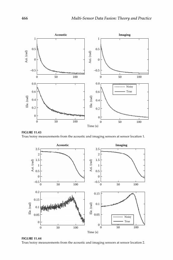
466 Multi-Sensor Data Fusion: Theory and Practice

FIGURE 11.44 True/noisy measurements from the acoustic and imaging sensors at sensor location 2.

Time (s)

00 50 100

0 50

Acoustic Imaging

NoisyTrue

100 0 50 100

0 50 100

0.05Ele.

(rad)

Azi. (

rad)

Azi. (

rad)

Ele.

(rad)

0.1

0.15

0.15

0.1

0.05

0

0.2

2.52

1.51

0.50

−0.5

2.52

1.51

0.50

−0.5

FIGURE 11.43 True/noisy measurements from the acoustic and imaging sensors at sensor location 1.

1Acoustic

50 100

Time (s)

0

Azi. (

rad)

0.5

0

−0.5

50 1000

Ele.

(rad)

0

0.2

0.4

0.6

0.8

50 100

NoisyTrue

0

Ele.

(rad)

0

0.2

0.4

0.6

0.8

1Imaging

50 1000

Azi. (

rad)

0.5

0

−0.5

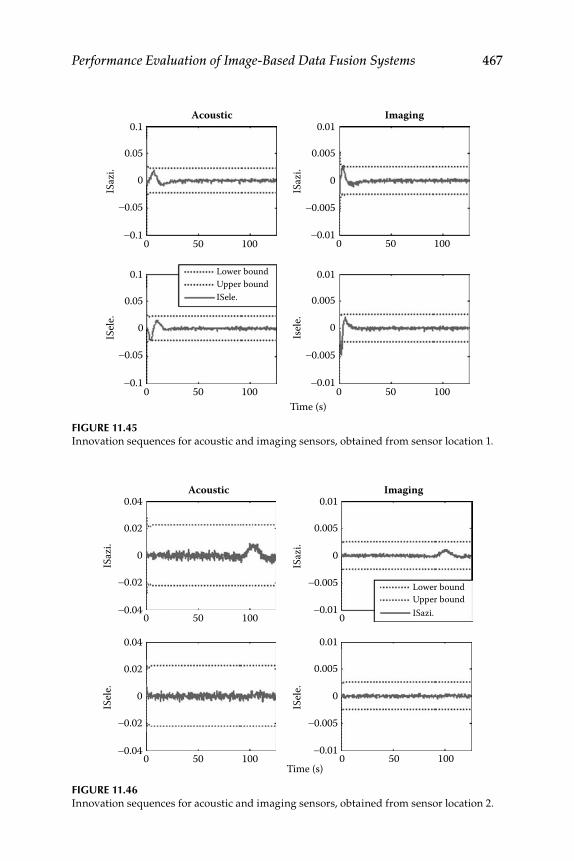
Performance Evaluation of Image-Based Data Fusion Systems 467

FIGURE 11.45 Innovation sequences for acoustic and imaging sensors, obtained from sensor location 1.

0.1 0.01

0.005

-0.005

-0.01

0

0.05

0

-0.05

ISaz

i.IS

ele.

Isele.

ISaz

i.

-0.1

-0.1

-0.05

0

0.05

0.1

0 50 100 0 50 100

-0.01

-0.005

0

0.005

0.01Lower boundUpper boundISele.

0 50 100 0Time (s)

50 100

Acoustic Imaging

FIGURE 11.46 Innovation sequences for acoustic and imaging sensors, obtained from sensor location 2.

0.04 0.01

0.005

0

-0.005 Lower boundUpper boundISazi.-0.01

0.01

0.005

0

-0.005

-0.01Time (s)

0.02

0

-0.02

-0.04

0.04

0.02

0

-0.02

-0.04

0 050 100

Acoustic

ISaz

i.IS

ele.

ISaz

i.IS

ele.

Imaging

0 50 100 0 50 100

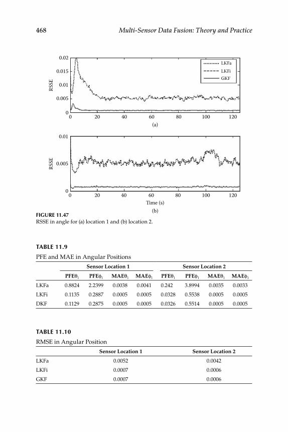
468 Multi-Sensor Data Fusion: Theory and Practice

TABLE 11.10

RMSE in Angular Position

Sensor Location 1 Sensor Location 2

LKFa 0.0052 0.0042

LKFi 0.0007 0.0006

GKF 0.0007 0.0006

FIGURE 11.47 RSSE in angle for (a) location 1 and (b) location 2.

0.02

0.015

RSSE

RSSE

0.01

0.01

0.005

0.005

00 20 40 60

(a)

(b)

80 100 120

LKFaLKFiGKF

00 20 40 60

Time (s)80 100 120

TABLE 11.9

PFE and MAE in Angular Positions

Sensor Location 1 Sensor Location 2

PFEθ1 PFEφ1 MAEθ1 MAEφ1 PFEθ1 PFEφ1 MAEθ1 MAEφ1

LKFa 0.8824 2.2399 0.0038 0.0041 0.242 3.8994 0.0035 0.0033

LKFi 0.1135 0.2887 0.0005 0.0005 0.0328 0.5538 0.0005 0.0005

DKF 0.1129 0.2875 0.0005 0.0005 0.0326 0.5514 0.0005 0.0005

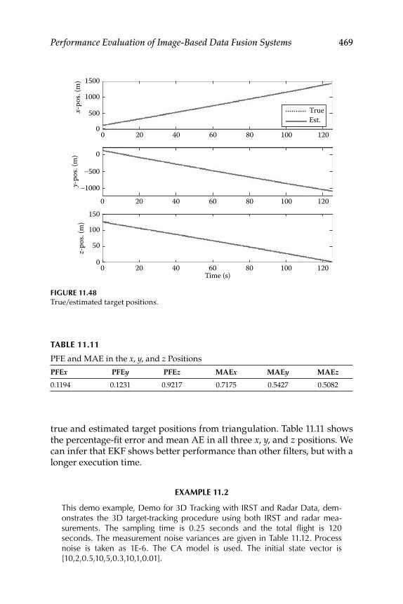
Performance Evaluation of Image-Based Data Fusion Systems 469

true and estimated target positions from triangulation. Table 11.11 shows the percentage-fi t error and mean AE in all three x , y , and z positions. We can infer that EKF shows better performance than other fi lters, but with a longer execution time.

EXAMPLE 11.2

This demo example, Demo for 3D Tracking with IRST and Radar Data, dem-onstrates the 3D target-tracking procedure using both IRST and radar mea-surements. The sampling time is 0.25 seconds and the total fl ight is 120 seconds. The measurement noise variances are given in Table 11.12. Process noise is taken as 1E-6. The CA model is used. The initial state vector is [10,2,0.5,10,5,0.3,10,1,0.01].

FIGURE 11.48 True/estimated target positions.

1500

1000

x-po

s. (m

)y-

pos.

(m)

z-po

s. (m

)

500

−500

−1000

150

100

50

00 20 40 60

Time (s)80 100 120

0

0

0 20 40 60 80 100 120

TrueEst.

0 20 40 60 80 100 120

TABLE 11.11

PFE and MAE in the x, y, and z Positions

PFEx PFEy PFEz MAEx MAEy MAEz

0.1194 0.1231 0.9217 0.7175 0.5427 0.5082

470 Multi-Sensor Data Fusion: Theory and Practice

SOLUTION 11.2 Run the MATLAB code ch11_ex2. The results are as follows:

PFEP : [0.0264 0.0386 0.3316]

PFEV : [0.1679 0.3524 2.0282]

PFEA : [1.7784 2.6751 18.1935]

MAEP : [0.4040 0.4129 0.2778]

MAEV : [0.0429 0.0501 0.0256]

MAEA : [0.0037 0.0036 0.0014]

RMSPE RMSVE RMSAE :[0.4867 0.0675 0.0070]

mean NIS : 4.9767

mean NEES : 7.7232

The various plots generated by this example are not included here in the text; however, when the program is run using MATLAB (in the command window), all of the plots are displayed.

TABLE 11.12

Measurement Variances (Example 11.2)

Sensor Azimuth (rad) Elevation (rad) Range (m)

IRST 1E-6 1E-6 –

Radar 1E-4 1E-4 10

471

Epilogue

There is a scope to adopt the unscented Kalman fi lter (derivative-free KF), or particle fi lter, with appropriate modifi cations, to track the centroid of the extended target, instead of the probabilistic data association fi lter (to replace the KF part). Different kinds of image-registration techniques are used in medical image processing. In some situations, the objects in the scene would be at different distances from the imaging sensor. Inex-pensive sensors would not properly focus everywhere. If one object is in focus, then another will be out of focus. This would yield a slightly out-of-focus fused image [13,37]. Multisensor image-fusion applications are treated in a study by Blum and Liu [38]. Although estimation fusion rules and algorithms (see Section 2.2) are very useful for target-tracking and fusion applications, their use in image-tracking applications (centroid tracking, etc.) is very limited. Further details on the development of image fusion and related tracking algorithms and applications can be found in [39–41].

Exercises

III.1. In what ways can the fusion of 3D vision data and active tactile sensing be useful?

III.2. In what ways can the fusion of vision information and ther-mal sensing be useful in object recognition and, hence, target tracking?

III.3. What are the merits of fusing information from laser radar (LADAR) and forward-looking infrared (FLIR) images?

III.4. Explain the difference between decision fusion and data fusion in the context of image fusion.

III.5. Consider an image fusion example and prove that decision fusion is a special case of data fusion.

III.6. How would you use the processes of data fusion and decision fusion in the context of acoustic- and vision-based information (say, for speech recognition)?

III.7. In light of the previous exercise, can you construct and show the scheme for the fusion of acoustic and visual information using artifi cial neural networks?

472 Multi-Sensor Data Fusion: Theory and Practice

III.8. What is the distinction between active and passive sensors in the context of visual sensors [40]?

III.9. What is an “active vision”?

III.10. What are passive imaging sensors/systems?

III.11. What are active sensing systems/techniques?

III.12. What are the intrinsic and extrinsic parameters of a camera?

III.13. Why is calibration of a camera necessary?

III.14. Explain the procedure of fusion of a stereo vision system.

III.15. Give examples of some fusion confi gurations (sensor network confi gurations) in the context of image/vision systems.

III.16. Why are image synchronization and registration important for the image-fusion process?

III.17. An RBF can be used in the transform model of the ABM for image registration (see Section 10.1.3.2). What then is the differ-ence between this method and the RBF neural network?

III.18. Which fusion rule (as discussed in Chapter 9) is implied by Equation 10.67 (see Section 10.3.4.1)?

III.19. Which rule for image fusion is implied by the algorithm given in Chapter 9?

III.20. Is it possible to model image noise as something other than linear additive noise?

III.21. Why is segmentation required in the process of image analysis/fusion?

III.22. What is actually the function of principal-component analysis or PCA?

III.23. What is implied by the formula of Equation 10.39? What are the weights?

III.24. What is implied by the formula of Equation 10.45? What are the weights?

III.25. If sensor 1 has an uncertainty ellipse with its major axis in the x direction and sensor 2 has an uncertainty ellipse with its major axis in the y direction, and if these 2D images are fused, what is the likely shape of the uncertainty ellipse?

III.26. What it the signifi cance of Exercise III.25?

III.27. What is the useful feature available in a thermal imager?

III.28. Do we get a 3D view of an image from a conventional television?

Performance Evaluation of Image-Based Data Fusion Systems 473

III.29. What type of sensory information do we obtain or use in pixel-level and feature-level fusion processes?

III.30. What type of sensory information do we use for pixel-level and feature-level image-fusion processes?

III.31. What are the registration aspects for pixel- and feature-level fusion algorithms or processes?

III.32. What is the fundamental fusion process for pixel- and feature-level image fusion?

III.33. What are the common noise sources that can contaminate an image?

III.34. What are possible methods for reducing the effect of noise pro-cesses in acquired images?

III.35. What are the spatial fi lter types and their fundamental characteristics?

III.36. What is the condition on the convolution mask in the case of the linear mean fi lters?

III.37. What are the main characteristics of nonlinear spatial fi lters?

III.38. What is “noise” in the context of an image?

III.39. What is “uncorrelated noise” in the context of an image?

III.40. What are the distinct noise processes in the context of an image?

III.41. What are the possible causes of noise in an image?

III.42. How is salt and pepper noise generated for an image?

III.43. What are the major types of image segmentation?

III.44. How is the image-registration algorithm used to help in target tracking?

III.45. When comparing two images for image registration, when is the sum of the absolute difference minimal?

III.46. While scanning an image, what is the difference between intrascan and interscan fi lters?

III.47. What are the fundamental requirements for fusion results in the case of image fusion?

III.48. What is the major signifi cance of image fusion from the view-point of a fused image?

III.49. What does spatial frequency do in the context of an image?

III.50. What is blocks-based image fusion?

III.51. What are multiwavelets, and how can they be used for image fusion?

474 Multi-Sensor Data Fusion: Theory and Practice

References

1. Hong, G. 2007. Image fusion, image registration, and radiometric normaliza-tion for high resolution image processing. PhD Thesis, TR No. 247, Department of Geodesy and Geomatics Engineering, University of New Brunswick, Fredericton, New Brunswick, Canada, p. 198.

2. Goshtasby, A. A. and S. Nikolov, eds. 2007. Image fusion: Advances in the state of the art. Inf Fusion 8:114–8.

3. Zitova, B., and J. Flusser. 2003. Image registration methods: A survey. Image Vis Comput 21:977–1000.

4. Gonzalez, R. C., and R. E. Woods. 1993. Digital image Processing . New York: Addison-Wesley Inc.

5. Hill, P., N. Canagarajah, and D. Bull. 2002. Image fusion using complex wave-lets. BMVC. http://www.bmva.ac.uk/bmvc/2002/papers/88/full_88.pdf (accessed December 2008).

6. Qu, J., and C. Wang. 2001. A wavelet package-based data fusion method for multi-temporal remote sensing image processing. 22 nd Asian conference on remote sensing, November 2001, Singapore.

7. Kumar, A., Y. Bar Shalom, and E. Oron. 1995. Precision tracking based on segmentation with optimal layering for imaging sensor. IEEE Trans Pattern Anal Mach Intell 17:182–8.

8. Oron, E., A. Kumar, and Y. Bar Shalom. 1993. Precision tracking with seg-mentation for imaging sensor. IEEE Trans Aerosp Electron Syst 29:977–87.

9. Waltz, E. and J. L. Llinas. 1990. Multi-sensor data fusion. Boston: Artech House.

10. Naidu, V. P. S., and J. R. Raol. 2008. Pixel-level image fusion using wave-lets and principal component analysis—A comparative analysis. Def Sci J 58:338–52.

11. Leung, L. W., B. King, and V. Nohora. 2001. Comparison of image fusion techniques using entropy and INI. 22 nd Asian conference on remote sensing, November 2001, Singapore.

12. Naidu, V. P. S., G. Girija, and J. R. Raol. 2007. Data fusion for identity estima-tion and tracking of centroid using imaging sensor data. Def Sci J 57:639–52.

13. Pajares, G., and J. M. de la Cruz. 2004. A wavelet-based image fusion tutorial. Pattern Recognit 37:1855–72.

14. Li, S., J. T. Kwok, and Y. Wang. 2001. Combination of images with diverse focuses using the spatial frequency. Inf Fusion 2:169–76.

15. Eskicioglu, A. M., and P. S. Fisher. 1995. Image quantity measures and their performance. IEEE Trans Commun 43:2959–65.

16. Cover, T. M., and J. A. Thomas. 1991. Elements of information theory . New York: Wiley.

17. Wang, Z., and A. C. Bovik. 2002. A universal image quality index. IEEE Signal Process Lett 9:81–4.

18. Cvejic, N., A. Loza, D. Bull, and N. Cangarajah. 2005. A similarity metric for assessment of image fusion algorithms. Int J Signal Process 2:178–82.

Performance Evaluation of Image-Based Data Fusion Systems 475

19. Piella, G., and H. Heijmans. 2003. A new quality metric for image fusion. Proceedings of the IEEE International Conference on Image Processing, Barcelona, Spain, pp. 173–6.

20. Jalili-Moghaddam, M. 2005. Real-time multi focus image fusion using dis-crete wavelet transform and Laplasican pyramid transform. Master’s thesis, Chalmess University of Technology, Goteborg, Sweden.

21. Daubechies, I. 1992. Ten lectures on wavelets. Regional conference series in applied maths , Volume 91. Philadelphia: SIAM.

22. Baltzakis, H., A. Argyros, and P. Trahanias. 2003. Fusion of laser and visual data for robot motion planning and collision avoidance. Mach Vis Appl 15:92–100.

23. Wang, J. G., K. A. Toh, E. Sung, and W. Y. Yau. 2007. A feature-level fusion of appearance and passive depth information for face recognition. In Face recognition , ed. K. Delac, and M. Grgic. Vienna, pp. 537–58, Austria: I-Tech.

24. Ross, A., and G. Rohin. 2005. Feature level fusion using hand and face biome-tircs. In Proceedings of SPIE conference on biometric technology for human identi-fi cation II , Vol. 5779, 196–204, Orlando, FL.

25. Chang, K. C., R. K. Saha, and Y. Bar-Shalom. 1997. On optimal track-to-track fusion. IEEE Trans Aerosp Electron Syst 33:1271–6.

26. Cheezum, M. K., W. F. Walker, and W. H. Guilford. 2001. Quantitative com-parison of algorithms for tracking single fl uorescent particles. Biophys J 81:2378–88.

27. Pratt, W. K. 1974. Correlation techniques of image registration. IEEE Trans Aerosp Electron Syst 10:353–8.

28. Chang, S., and C. P. Grover. 2002. Centroid detection based on optical cor-relation. Opt Eng 41:2479–86.

29. Romine, J. B., and E. W. Kamen. 1996. Modeling and fusion of radar and imaging sensor data for target tracking. Opt Eng 35:659–72.

30. Naidu, V. P. S., G. Girija, and J. R. Raol. 2005. Target tracking and fusion using imaging sensor and ground based radar data, AIAA guidance, navi-gation and control conference and exhibit, Paper No. AIAA-2005-5842, San Francisco, CA.

31. Dogancay, K., and A. Hashemi-Sakhtsari. 2005. Target tracking by time dif-ference of arrival using recursive smoothing. Signal Process 85:667–79.

32. Stoica, P., and A. Nehorai. 1989. MUSIC, maximum likelihood, and Cramer-Rao bound. IEEE Trans Acoust Speech Signal Process 37:720–41.

33. Johnson, D. H., and D. E. Dudgeon. 1993. Array signal processing: Concepts and techniques . Prentice Hall Signal Processing Series . Englewood Cliffs, NJ: Prentice Hall.

34. Wijk, O., and H. I. Christensen. 2000. Triangulation-based fusion of sonar data with application in robot pose tracking. IEEE Trans Rob Autom 16:740–52.

35. Dufour, F., and M. Mariton. 1991. Tracking a 3D maneuvering target with passive sensors. IEEE Trans Aerosp Electron Syst 27:725–38.

36. Naidu, V. P. S., and J. R. Raol. 2007. Target tracking with multiacoustic array sensors data. Def Sci J 57(3):289–303.

37. Strobel, N., S. Spors, and R. Rabenstein. 2001. Joint audio-video object localization and tracking. IEEE Signal Process Mag 18:22–31.

476 Multi-Sensor Data Fusion: Theory and Practice

38. Naidu, V. P. S., and J. R. Raol. 2008. Fusion of out of focus images using principal component analysis and spatial frequency. J Aerosp Sci Technol 60:216–225.

39. Blum, R. S., and Z. Liu. 2006. Multi-sensor image fusion and its applications . Boca Raton, FL: CRC Press.

40. Harris, C., A. Bailey, and T. Dodd. 1998. Multisensor data fusion in defense and aerospace. J Aerosp Soc 162:229–44.

41. Naidu, V. P. S., M. Mudassar, G. Girija, and J. R. Raol. 2005. Target location and identity estimation and fusion using disparate sensor data, AIAA guid-ance, navigation and control conference and exhibit, Paper No. AIAA-2005-5841, San Francisco, CA.

42. Sam Ge, S., and F. L. Lewis, eds. 2006. Autonomous mobile robots—Sensing, con-trol, decision making and applications. Control engineering series . Boca Raton, FL: CRC Press.

IV Part

A Brief on Data Fusion in Other Systems

A. Gopal and S. Utete

479

12Introduction: Overview of Data Fusion in Mobile Intelligent Autonomous Systems

12.1 Mobile Intelligent Autonomous Systems

Intelligent fi eld robotic systems are mobile robots that operate in an uncon-strained and dynamic environment. Unlike their conventional manufac-turing counterparts that operate in controlled environments, fi eld robotic systems are more challenging due to the signifi cantly more complex lev-els of perception, navigation, planning, and learning required to achieve their missions [1].

Perception addresses the challenges associated with understanding the environment in which the robotic system is operating. Environmen-tal understanding is achieved through the creation of models that are truthful representations of the robotic system’s operating environment. Many types of sensors can be used for this world-modeling task, includ-ing sonar, laser scanners, and radar (see Section 2.5); however, the pri-mary focus of a mobile intelligent autonomous system (MIAS) within the perception research domain is to acquire and interpret visual data. Navi-gation uses the knowledge of the perceived environment as well as addi-tional information from other on-board sensors to address the challenges of localizing the system within the environment and controlling the platform actuators to maintain a given trajectory. Mapping an unknown environment while simultaneously localizing within that environment is also part of the navigation challenge. Planning addresses the challenge of integrating the knowledge of the high-level goals with the current system perception and localization to generate appropriate behaviors that will take the system closer to successfully achieving these goals. The objective of planning is to generate behavior options and then decide which behav-ior will be executed. Finally, learning closes the loop by incorporating the knowledge of previous states, behaviors, and results in order to improve the system’s reasoning capability and increase the probability of choosing the optimal behavior.

480 Multi-Sensor Data Fusion: Theory and Practice

These four MIAS areas overlap, to some degree, with the common thread among them being suitable knowledge representation. A unifi ed frame-work defi nition for interfaces and data fl ow (system architecture) is also required to facilitate the integration of all MIAS subsystems into a single demonstrator system. It is at this system-level integration that the benefi ts of data fusion will be most noticeable. The distinguishing characteristic of MIAS is that these systems operate in an environment that changes, often unpredictably, and as a result they have to fi rst detect the change and then assess the impact of the change on their task or objective. Depending on the result of the assessment, the system must make appropriate plan-ning and actuation decisions to compensate for the change while still achieving its objective.

Examples of MIAS global research include the following (Figure 12.1): (1) the driverless car and underground mine safety initiatives at the Council

(a) (b) (c)

(d) (e)

FIGURE 12.1 Some systems where data fusion and AI could play major role: (a) Driverless vehicle research

platforms (from www.csir.co.za/mias. With permission.); (b) Sony’s QRIO humanoid (from

en.wikipedia.org/wiki/Qrio. With permission.); (c) Honda’s Asimo humanoid (photo taken

by the author at the Auto Africa motor show in South Africa); (d) Israel Aircraft Industries’

RQ-2 Pioneer UAV (from en.wikipedia.org/wiki/RQ-2_Pioneer. With permission.); and

(e) Bluefi n-12 AUV/Bluefi n Robotics in the USA. (from en.wikipedia.org/wiki/AUV. With

permission.)

Introduction: Overview of Data Fusion in MIAS 481

for Scientifi c and Industrial Research (CSIR), South Africa, (2) QRIO of Sony, (3) Honda’s Asimo humanoid programs, (4) unmanned military ground and air vehicles, and (5) the Bluefi n-12 autonomous underwater vehicle (AUV) from Bluefi n Robotics in the United States.

12.2 Need for Data Fusion in MIAS

There are several reasons for data fusion in MIAS: (1) the environment in which the system is operating is not always fully observable; (2) the interpretation of the environment is done via sensors (and only one sen-sor will not provide complete information about the scene); (3) in many instances, some information is uncertain; (4) the real world is spatially and temporally linked, and data fusion provides a useful methodology for realizing this relationship [2]. A good example of an environment that is not fully observable is a cluttered environment with many obstacles to obscure sensors, in which a mobile robot needs to navigate, or when a mobile robot must navigate to a point that is beyond the range of its exterioceptive sensors. In this case, fusing the system localization with an a priori map of the environment will facilitate better path-planning strate-gies in order to reach the destination point.

Mobile robots rely on sensors to generate a description of internal states and the external environment. Internal state sensors are referred to as proprioceptive sensors , and sensors for measuring the external environ-ment are referred to as exterioceptive sensors [3]. Proprioceptive sensors are typically used to measure robot velocity, acceleration, attitude, current, voltage, temperature, and so on, and are used for condition monitoring (fault detection), maintaining dynamic system stability, and controlling force/contact interaction with the external environment. Exterioceptive sensors are typically used to measure range, color, shape, light intensity, and so on, and are used to construct a world model in order to interact with the environment through navigation or direct manipulation. These sensors measure very specifi c information such as range and color and thus provide only partial views of the real world, which need to be fused together in order to provide a complete picture. Also, the information that needs to be fused does not need to be limited to a numerical format as is typical of measurement sensors, but can be linguistic or in other formats, which allows the system to build a more descriptive world model that can be used to determine if the end objective has been achieved.

In addition, data fusion increases prediction accuracy and the robust-ness of information and reduces noise and uncertainty. Dead-reckoning errors for mobile robot localization are cumulative, and fusion with exterioceptive sensor information is required to determine the robot’s

482 Multi-Sensor Data Fusion: Theory and Practice

location more accurately. Data fusion also facilitates the detection and extraction of patterns that are not present in the unfused data and is therefore very useful for system condition monitoring and target track-ing. Lastly, robotic systems operating under a decentralized processing architecture require data fusion to incorporate data communicated from neighboring nodes with local observations [4].

12.3 Data Fusion Approaches in MIAS

Data fusion in mobile robotics occurs at different levels: (1) time series data fusion of a single sensor, (2) fusion of data from redundant sensors, (3) fusion of data from multiple sensors, and (4) fusion of sensor and goal information. Each level of fusion has challenges associated with it that depend on the type of data being fused, the requirements of the applica-tion, and the reliability of the outputs.

Approaches to data fusion in MIAS applications generally include (1) statistical analysis, such as the Kalman fi lter, (2) heuristic methods, such as Bayesian networks, (3) possibility models, such as fuzzy logic and Dempster–Shafer, (4) mathematical models, (5) learning algorithms based on neural networks, (6) genetic algorithm-type evolutionary algorithms, and (7) hybrid systems [5].

A brief overview of some of the research being conducted internation-ally is presented here to give the reader a broad perspective of the fi eld. It is not intended to be a comprehensive mathematical description of all available data fusion methods, many of which have been covered in the preceding sections of the book.

The Kalman fi lter–based approach to data fusion is probably the most signifi cant and widely studied method to date. It depends on linear state-space models and Gaussian probability density functions; the extended Kalman fi lter is based on a Jacobian linearization and can be applied to nonlinear models. However, errors introduced in the linearization pro-cess in real applications such as navigation, where the underlying process is typically nonlinear, can cause inaccuracies in the state-vector fusion approach. Reference 3 asserts that in these cases the measurement fusion approach is preferred to state-vector fusion. Measurement fusion directly fuses sensor data to obtain a weighted or augmented output, which can then be input into a Kalman fi lter. The data from multiple sensors is com-bined using weights to reduce the mean-square-error estimate, and the dimension of the observation vector remains unchanged. In the state-vector approach, data from multiple sensors are added to the observation vector and result in an increased dimension. A separate Kalman fi lter is

Introduction: Overview of Data Fusion in MIAS 483

required for each sensor observation, and the results of the individual estimates are then fused to give an improved estimate. According to [3], the state-vector fusion method is computationally more effi cient, but the measurement fusion method has more information and should be more accurate; the net result is that both methods are theoretically function-ally equivalent, if the sensors have identical measurement matrices (see Section 3.1).

An example of Kalman fi lter–based fusion is described in [6], where the issue of cumulative errors in odometry for localization is addressed through the fusion of laser range data and image intensity data. An extended Kalman fi lter is used to determine the location of vertical edges, corners, and door and window frames, which is then compared to an a priori map to obtain a better estimation of the robot’s location. The Kalman fi lter is also used to fuse laser and stereo range data to model the environ-ment using 3D planes [7].

Bayesian estimators were very prominent in earlier works on sensor fusion for mobile robot applications, but research with this method had been stagnant for years before again increasing in popularity recently. Some researchers use Bayesian estimators to fuse sonar and stereovision range data for marking cells in an occupancy grid as occupied, empty, or unknown.

Examples of mathematics-based data fusion methods include exponential mixture density (EMD) models and vector fi eld histograms. In [8], the theo-retical properties of exponential mixture density models are investigated to determine their applicability to robust data fusion in distributed networks. These developments take advantage of the previous use of EMDs in expert data fusion and the adaptation of nonlinear fi ltering methods, such as par-ticle fi lters, to suit the EMD ’s computational requirements and develop upper and lower bounds on the probabilities of the result. The authors claim a consistent and conservative data fusion method for information with unknown correlations. In [9], evidence grid methodology, also referred to as occupancy grids, certainty grids, or histogram grids, is used for naviga-tion in conjunction with vector fi eld histograms (VFHs) to fuse CCD camera data and laser rangefi nder data. Data fusion was successfully demonstrated on the navigator wheeled platform. Evidence grid methodology can also implement probabilistic measurements as demonstrated by Martin and Moravec from Carnegie Mellon University (cited in [9]). Approaches based on possibility theory data fusion center around the application of fuzzy logic theory (see Chapter 6). The use of neural networks and genetic algo-rithms for data fusion are also possible applications in MIAS.

Research in data fusion is also being conducted from the system archi-tecture perspective; in [5], a general data fusion architecture based on the unifi ed modeling language (UML) is developed that allows for dynamic changes in the framework in order to respond to changes in a dynamic

484 Multi-Sensor Data Fusion: Theory and Practice

environment. This approach introduces taxonomy for data fusion and facilitates various levels of fusion.

The current challenges in data fusion for MIAS are in the character-ization of uncertainty as well as vagueness in sensor measurements [3]. The problem of quantitative gain from data fusion to justify the cost implications of additional sensors must also be addressed. A good chal-lenge in MIAS is that of the SLAM (simultaneous localization and map-ping), which uses extended Kalman fi lter and data association methods and applications to multirobot systems, mining robot arms that can take advantage of the data fusion approaches discussed in the previous sec-tions of the book. The real challenge is in building MIAS so that the system not only carries out its various tasks rationally, but also thinks rationally, like a human being!

485

13 Intelligent Monitoring and Fusion

Data fusion has an extensive range of applications in aeronautics, space systems, and robotics. It also has applications in monitoring the health or condition of systems [10], where fusion can be used to improve the obser-vations made about a system or environment for event detection. This section considers various aspects that contribute to the development of intelligent monitoring and fusion systems—systems capable of making decisions about the existence of precursors to events through the acquisi-tion and combination of data about an environment or system.

Condition monitoring involves the acquisition and analysis of data to determine changes in an observed system or environment. Examples include the monitoring of systems, such as jet engines, for preventive maintenance purposes [11,12] and the monitoring of environments, such as mine work areas, as described in [13]. Condition monitoring can involve the processing of data for fault characterization, change detection, or nov-elty or anomaly detection [12]. In novelty detection, a model or description of the normal state of the observed system or environment is developed. Changes from this model or description are then detected. This approach is important for high-integrity systems, such as aircraft engines, where faults by defi nition are few.

Other applications of condition monitoring include multiple-server moni toring, which is relevant to companies such as Web search entities. In robotics, condition-monitoring applications can be used for the manage-ment of fl eets of robots or in the use of mobile robots as sensor platforms to make observations in mining environments (Candy, L., June 2008, pers. comm ).

13.1 The Monitoring Decision Problem

Intelligent monitoring and fusion involve the combination of data acquired by intelligent agents, such as intelligent sensors, which make observa-tions of a system or environment in order to detect precursors to events or anomalies. Monitoring involves a decision problem about the presence or absence of events through the detection of changes in the state, which are

486 Multi-Sensor Data Fusion: Theory and Practice

indicative of an underlying change in the system. Detection of anomalies is required at an early stage, before events occur, so that action can be taken, if necessary.

In offl ine condition monitoring, data can be batched, and decision making can take place once a predetermined set of data has been acquired (Figure 13.1); this is essentially a centralized data and decision fusion scheme. In online condition monitoring, data must be examined and classifi ed as it is being acquired, and a delayed decision might be of little value. For large volumes of data, online monitoring bears some resem-blance to stream data-processing problems, which arise, for example, in the management and analysis of network traffi c [14].

Given the time limits of online monitoring, suboptimal strategies for data analysis and decision making are relevant to event detection. One method with a potential application is ordinal optimization [15]. Ordinal optimization can be employed to reduce the size of the data set that must be examined to achieve a goal [15]. Given the restricted time available to examine the data in online monitoring, one approach is to develop robust decision methods that utilize subsets of representative data or can provide a decision about the state of a data stream, rather than computing estimates explicitly. Abstraction of data, as in voting [16], is also potentially useful.

Table 13.1 compares a single sonar sensor’s beliefs about the target type with a fusion of the beliefs of 15 such sensors using Dempster’s rule [14]. For a description of Dempster–Shafer reasoning, see [17] and Section 2.3. The sensors seek to differentiate between planes and corners. At both of the tabulated angular positions, the multisensor system outperforms the single sensor in terms of classifi cation accuracy. The performances of the sensor groups using Dempster’s fusion rule and voting are compared in Table 13.2. In each case, fi ve sensors are grouped, and their beliefs are fused. For these groups of distributed sensors, voting gives a higher per-centage of correct decisions. This can be explained by voting’s relative insensitivity to the confl icting decisions of the sensors in the selected groups [16]. For some monitoring tasks, the number of sensors supporting

FIGURE 13.1 Batched processing method for offl ine monitoring.

Monitoring/decisionprocess Data fusionAcquire data Decision

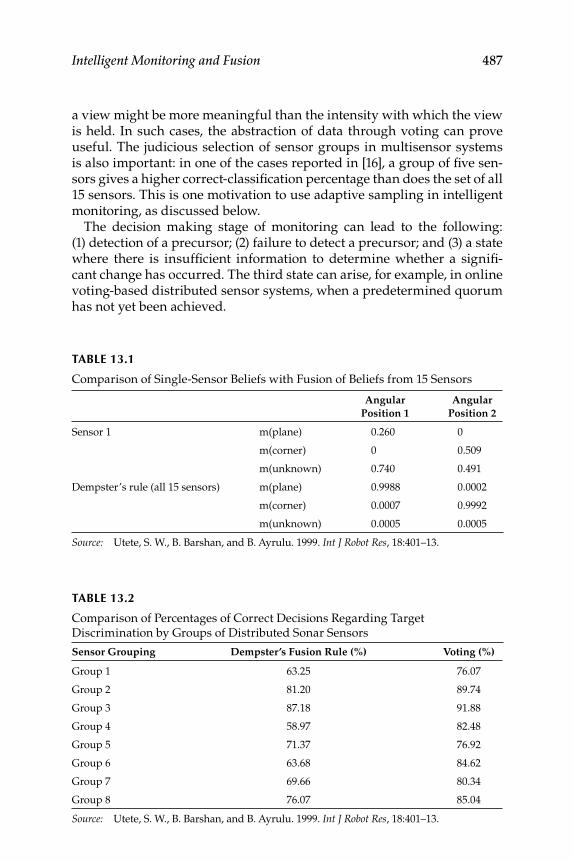
Intelligent Monitoring and Fusion 487

a view might be more meaningful than the intensity with which the view is held. In such cases, the abstraction of data through voting can prove useful. The judicious selection of sensor groups in multisensor systems is also important: in one of the cases reported in [16], a group of fi ve sen-sors gives a higher correct-classifi cation percentage than does the set of all 15 sensors. This is one motivation to use adaptive sampling in intelligent monitoring, as discussed below.

The decision making stage of monitoring can lead to the following: (1) detection of a precursor; (2) failure to detect a precursor; and (3) a state where there is insuffi cient information to determine whether a signifi -cant change has occurred. The third state can arise, for example, in online voting-based distributed sensor systems, when a predetermined quorum has not yet been achieved.

TABLE 13.1

Comparison of Single-Sensor Beliefs with Fusion of Beliefs from 15 Sensors

Angular

Position 1

Angular

Position 2

Sensor 1 m(plane) 0.260 0

m(corner) 0 0.509

m(unknown) 0.740 0.491

Dempster’s rule (all 15 sensors) m(plane) 0.9988 0.0002

m(corner) 0.0007 0.9992

m(unknown) 0.0005 0.0005

Source: Utete, S. W., B. Barshan, and B. Ayrulu. 1999. Int J Robot Res, 18:401–13.

TABLE 13.2

Comparison of Percentages of Correct Decisions Regarding Target Discrimination by Groups of Distributed Sonar Sensors

Sensor Grouping Dempster’s Fusion Rule (%) Voting (%)

Group 1 63.25 76.07

Group 2 81.20 89.74

Group 3 87.18 91.88

Group 4 58.97 82.48

Group 5 71.37 76.92

Group 6 63.68 84.62

Group 7 69.66 80.34

Group 8 76.07 85.04

Source: Utete, S. W., B. Barshan, and B. Ayrulu. 1999. Int J Robot Res, 18:401–13.

488 Multi-Sensor Data Fusion: Theory and Practice

13.2 Command, Control, Communications, and Configuration

Athans poses control problems arising in C2 and C3 systems and makes a case for the adaptation of methods from the command, control, and com-munication theory for civilian applications. Note that issues in condition-monitoring problems resemble the problems in situational assessment. Incorporating situational assessment into intelligent monitoring would be an example of the type of crossover proposed by Athans [18].

C3 systems are constrained by a fourth “C,” confi guration. In situations where a system of intelligent sensors or agents exchange information on a network, the network confi guration becomes a part of the information-processing paradigm, with potential implications for decision making, as in the case reported in [19]. The area of what might be termed “4C” systems is relevant to the development of robust methods for updating information, decision, and position in highly autonomous networks of sensor nodes or agents that collaborate to collect information about an observed environment.

Some of the issues that arise in this scenario are (1) the structure of the system through which decisions are communicated [20,21], (2) suboptimal strategies for decision making in highly autonomous networks [19], and (3) novelty detection by distributed agents.

Methods from graph theory can be applied to address network confi guration issues. For example, detecting a change of state using physical agents such as sensors is similar to early bird synchroniza-tion problems in automata theory [22]; this can be considered a physical novelty-detection problem. Results from extremal graph theory [23] and automata theory [22] can assist in understanding the questions that can be posed on particular network confi gurations [19]. It is also possible to draw on these areas for the analysis and development of sensor systems for intelligent monitoring.

13.3 Proximity- and Condition-Monitoring Systems

Awareness of confi guration is relevant to civilian situation-assessment applications, such as the proximity-detection systems of AcuMine products [24]. A proximity-monitoring network is an example of a 4C sys-tem. In AcuMine products [24], vehicle updates can be coordinated by a base station through interaction with other mobile units. The mobile units and the base station form a distributed system of monitoring agents (in this case, making observations about proximity and threats during task

Intelligent Monitoring and Fusion 489

performance). The system can also operate without the base unit, a situa-tion that creates a higher degree of autonomy for individual units and an accompanying need for greater levels of situational awareness and coor-dination. Position updates in such systems are relevant in terms of the decisions that can be made as the autonomy of mobile units increases. Wider applications can be made in other problems of multiple-robot or multiple-agent coordination.

Adaptive sampling systems are reactive systems [25] that respond strategically to the availability of relevant data; sampling occurs in response to changes in the information content. Spatial adaptive sam-pling systems have been developed for applications such as ocean monitoring [25].

Network-monitoring sensor systems have been developed for mine environment monitoring in the Council for Scientifi c and Industrial Research (CSIR) Mining Group’s AziSA project (CSIR NRE Mining, 2008, pers. comm). Both the AziSA system and AcuMine’s proximity- management systems [24] incorporate instances of adaptive sampling as follows: (1) Considering the diffi cult environmental conditions in under-ground mines and limitations to access, low-power sensors are required [CSIR NRE Mining, 2008, pers. comm.; Vogt, D., May 2008, pers. comm.]. In the case of the CSIR Mining Group’s AziSA network, the possibility of sleep–wake states for sensors has been considered [12]. Such states are an explicit instance of adaptive sampling. (2) Vehicles in the proximity- management system of AcuMine products [24] use an adaptive sampling time to inform other units of their most recent data acquisition. The demands of environmental monitoring necessitate that sensor nodes be active only in the presence of relevant new information. Adaptive sam-pling by sensor networks is an explicit form of novelty detection.

In an intelligent monitoring system, the processes of fusion and decision making can be augmented with position or sampling rate updates, as in Figure 13.2. Data is fused when it is acquired, and the processed values are used to generate a decision about the presence or absence of precur-sors. This information can be used to determine whether to increase or maintain the active rate of data sampling. In such dynamic monitoring systems, this decision could be about the position updates required from sensing platforms. Intelligent monitoring requires the development of techniques for adaptively sampling a monitored environment in order to focus attention and energy for data acquisition on the most information-rich spatial regions and time slots. This problem is fundamentally linked to condition monitoring in a wide range of contexts. Problems in sensor-network organizations, such as those discussed by Utete et al. [16], can also be related to this framework.

Thus, some aspects contributing to intelligent monitoring and fusion systems have been highlighted, with a special application to robotics. The

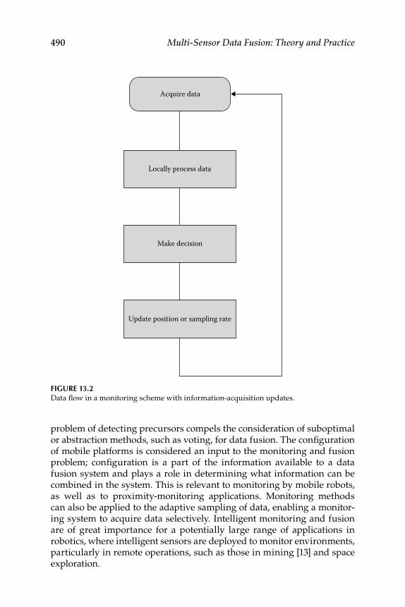
490 Multi-Sensor Data Fusion: Theory and Practice

problem of detecting precursors compels the consideration of suboptimal or abstraction methods, such as voting, for data fusion. The confi guration of mobile platforms is considered an input to the monitoring and fusion problem; confi guration is a part of the information available to a data fusion system and plays a role in determining what information can be combined in the system. This is relevant to monitoring by mobile robots, as well as to proximity-monitoring applications. Monitoring methods can also be applied to the adaptive sampling of data, enabling a monitor-ing system to acquire data selectively. Intelligent monitoring and fusion are of great importance for a potentially large range of applications in robotics, where intelligent sensors are deployed to monitor environments, particularly in remote operations, such as those in mining [13] and space exploration.

FIGURE 13.2 Data fl ow in a monitoring scheme with information-acquisition updates.

Update position or sampling rate

Make decision

Locally process data

Acquire data

491

Epilogue

Mobile intelligent autonomous systems (MIAS), a more general subject than robotics, is an emerging research area in many developing countries. The main research and development (R&D) issues involved are the follow-ing: (1) perception and reasoning, (2) mobility and navigation, (3) haptics and teleoperation, (4) image fusion and computer vision, (5) mathematical modeling of manipulators, (6) hardware and software architectures for planning and behavior learning, (7) path- and motion-planning of a robot or vehicle, and (8) the application results of artifi cial neural networks, fuzzy systems, probabilistic reasoning, Bayesian networks, and genetic algorithms to the above problems. Multisensor data fusion can play a very crucial role at many levels of the data fusion process, such as kinematic fusion (position/bearing tracking), image fusion (for scene recognition, building a world model), and decision fusion (for tracking and control actions). Many of the concepts, techniques, and algorithms discussed in Parts I, II, and III of this book are very much applicable to robotics and to MIAS, an emerging technology. Such systems are useful for the automation of complex tasks, surveillance in hazardous and hostile envi-ronments, human-assistance systems for very diffi cult manual activities, medical robotics, hospital systems, autodiagnostic systems, and many other related civil and military systems. It is important to understand the environment in which robotics and other intelligent systems operate, as they make decisions in the context of this environment in order to achieve their goals. Perception occurs when a robotic system or intelligent agent uses its sensors to acquire sensory information about its surroundings and then interprets this information to create models of its environment, which provide a truthful representation of that environment. Reasoning is the process by which a robotic system or intelligent agent incorporates new perceptions about its environment into its current knowledge and belief representations and uses its total knowledge to decide which actions to carry out in order to achieve its goals. Research areas include sensors and sensor modeling, computer vision, scene understanding, tactile sensing, human–machine interfaces, knowledge representation, learning, decision making, planning, and logic. Knowledge in the disciplines of statistical modeling, artifi cial intelligence, machine learning, pattern recognition, statistical learning methods, probabilistic reasoning, algorithmic design, and computer science are useful tools for researching MIAS technology.

Mobility addresses the physical issues in moving the system between points A and B. Navigation addresses issues related to planning the motion of the system to achieve mobility, as well as accomplishing

492 Multi-Sensor Data Fusion: Theory and Practice

mobility in the most effi cient way as measured against performance crite-ria such as energy or time. Localization, path planning, low-level obstacle avoidance, and map building are also very important issues. Haptics and teleoperation address issues in human–machine interfaces, with a focus on teleoperation using haptic feedback. Research on reality augmenta-tion, human response to tactile and visual stimuli, real-time feedback control, and 3D visualization are also very important research areas. The dynamic systems considered could be autonomous systems, fi eld robots, mobile/fi xed systems, mini/microrobots, mining robots, surveillance systems, networked/multirobot systems, and so on. The importance of this fi eld calls for a separate volume on data fusion for autonomous intel-ligent systems.

Exercises

IV.1. In what ways are inertial navigation systems, global positioning systems integration, and data fusion (Section 4.5) useful to a mobile robot?

IV.2. What are the three most important and major aspects of robotic architecture?

IV.3. What is the importance of each of the tasks in Exercise IV.2?

IV.4. What is map building for an autonomous robot? How would sensor data fusion be useful in this process?

IV.5. What roles can neural networks, fuzzy logic, and genetic algorithms play in an autonomous robotic system?

References

1. Sam Ge, S., and F. L. Lewis, eds. 2006. Autonomous mobile robots—Sensing, con-trol, decision making and applications (Control Engineering Series). Boca Raton, FL: CRC Press.

2. Vitko, A. 2008. Data fusion, context awareness and fault detection in autono-mous robotics, Faculty of Electrical Engineering and Information Technology, Institute of Control and Industrial Informatics, Slovakia.

3. Hu, H., and J. Q. Gan. 2005. Sensors and data fusion algorithms in mobile robotics, Technical report: CSM-422, Department of Computer Science, University of Essex, United Kingdom.

Intelligent Monitoring and Fusion 493

4. Durrant-Whyte, H. 2000. A beginners guide to decentralised data fusion, Australian Centre for Field Robotics, The University of Sydney, Australia.

5. Carvalho, H. S., W. B. Heinzelman, A. L. Murphy, and C. J. N. Coelho. 2003. A general data fusion architecture. In Proceedings of the Sixth International Conference of Information Fusion, 2:1465–72.

6. Neira, J., J. D. Tardos, J. Horn, and G. Schmidt. 1999. Fusing range and inten-sity images for mobile robot localisation. IEEE Trans Rob Autom 15:76–83.

7. Grandjean, P., and A. R. Robert de Saint Vincent. 1989. 3-D modeling of indoor scenes by fusion of noisy range and stereo data. In Proceedings of the IEEE International Conference in Robotics and Automation, 681–687, Scottsdale, AZ.

8. Julier, S. J., T. Bailey, and J. K. Uhlmann. 2006. Using exponential mixture models for suboptimal distributed data fusion. In Proceedings of the Nonlinear Statistical Signal Processing Workshop, 160–163. UK: IEEE.

9. Conner, D.C., P. R. Kedrowski, and C. F. Reinholtz. 2001. Multiple camera, laser rangefi nder, and encoder data fusion for navigation of a differentially steered 3-wheeled autonomous vehicle. In Proceedings of SPIE, 4195:76–83, Bellingham, WA.

10. Raheja, D., J. Llinas, R. Nagi, and C. Romanowski. 2006. Data fusion/data mining-based architecture for condition based maintenance. Int J Prod Res 44:2869–87.

11. Nairac, A., N. Townsend, R. Carr, S. King, P. Cowley, and L. Tarassenko. 1999. A system for the analysis of jet engine vibration data. Integr Comput Aided Eng 6:53–66.

12. Hayton, P., S. Utete, D. King, S. King, P. Anuzis, and L. Tarassenko. 2007. Static and dynamic novelty detection methods for jet engine condition moni-toring. In Philosophical Transactions of the Royal Society Part A . Special Issue on Structural Health Monitoring, ed. K. Worden and C. Farrar, 365:493–514. London: The Royal Society.

13. Vogt, D., and V. Z. Brink. 2007. The Azisa standard for mine sensing and control. Presentation at Automation in Mining Conference.

14. Hayes, B. 2008. The Britney Spears problem. Am Sci 96:274–9. 15. Ho, Y.-C. 1994. Heuristics, rules of thumb, and the 80/20 proposition. IEEE

Trans Automat Contr 39:1025–7. 16. Utete, S. W., B. Barshan, and B. Ayrulu. 1999. Voting as validation in robot

programming. Int J Robot Res 18:401–13. 17. Krause, P., and D. Clark. 1993. Representing uncertain knowledge: An artifi cial

intelligence approach . Oxford: Intellect Books. 18. Athans, M. 1987. Command and control (C2) theory: A challenge to control

science. IEEE Trans Automat Control 32:286–93. 19. Utete, S. 1994. Network Management in Decentralised Sensing Systems, PhD

Thesis, Department of Engineering Science, University of Oxford, UK. 20. Grime, S. 1992. Communication in Decentralised Sensing Architectures. PhD

Thesis, Department of Engineering Science, University of Oxford, UK. 21. Grime, S., and H. F. Durrant-Whyte. 1994. Data fusion in decentralised sensor

networks. Control Eng Pract 2:849–63. 22. P. Rosenstiehl, J. R. Fiksel, and A. Holliger. 1972. Intelligent graphs: networks

of fi nite automata capable of solving graph problems. In Graph theory and computing , ed. R. Read. London: Academic Press.

494 Multi-Sensor Data Fusion: Theory and Practice

23. Bollobás, B. 1978. Extremal graph theory . London: Academic Press. 24. AcuMine products. 2008. http://www.acumine.com/_Products/products.php

(accessed January 2009). 25. Ehrich Leonard, N., D. A. Paley, F. Lekien, R. Sepulchre, D. M. Fratantoni, and

R. E. Davis. 2007. Collective motion, sensor networks, and ocean sampling. Proc IEEE 95.

495

Appendix: Numerical, Statistical, and Estimation Methods

Data fusion (DF) could become a core technology for current and future onboard data-processing schemes in many aerospace and ground-based systems. DF is based on many theories, concepts, and methods, such as signal processing, control and estimation theory, artifi cial intelligence, pattern recognition, spectral analysis, reliability theory, statistical tools, wavelet analysis, artifi cial neural networks (ANNs), fuzzy logic (FL), genetic algorithms (GAs), knowledge-based expert systems, and decision theory [1–12]. In essence, we can obtain combined information with higher-quality and refi ned data and thus can eliminate redundancy. Statistical matching is often used as a core fusion algorithm. The approach can be compared to the k –NN (nearest neighbor) prediction with two sets of data: the training set and the test set. The Euclidian distance is used as a measure for matching the distance. A prediction of the fusion variables is made using the set of nearest neighbors found. Nearest neighbors are found by computing averages, modes, or distributions. The training set data could be a very large sample of the general population; the train-ing set variables should be good predictors for the fusion variables. For numerical data, the methods of estimation theory are directly adaptable to the DF problem, as discussed in Section 2.2.

A.1 Some Definitions and Concepts

Several defi nitions and concepts that are useful in data processing and DF are compiled here [1–3].

A.1.1 Autocorrelation Function

For x ( t ), a random signal

Rxx(τ) = E{x(t)x(t + τ)} (A.1)

Here, τ is the time lag and E is the mathematical expectation operator. If Rxx decreases with an increase in time, this means that the nearby val-ues of the signal x are not correlated. The autocorrelation of the white

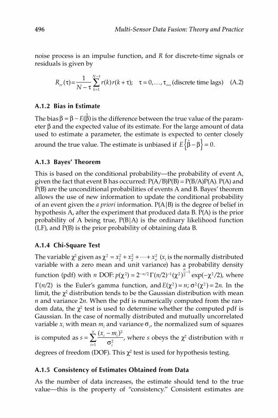
496 Multi-Sensor Data Fusion: Theory and Practice

noise process is an impulse function, and R for discrete-time signals or residuals is given by

Rrr (τ)= 1

N − τr(k)

k=1

N −τ

∑ r(k + τ); τ = 0,K, τmax

(discrete time lags) (A.2)

A.1.2 Bias in Estimate

The bias β = β − E(β) is the difference between the true value of the param-eter β and the expected value of its estimate. For the large amount of data used to estimate a parameter, the estimate is expected to center closely

around the true value. The estimate is unbiased if E β − β{ } = 0.

A.1.3 Bayes’ Theorem

This is based on the conditional probability—the probability of event A, given the fact that event B has occurred: P(A/B)P(B) = P(B/A)P(A). P(A) and P(B) are the unconditional probabilities of events A and B. Bayes’ theorem allows the use of new information to update the conditional probability of an event given the a priori information. P(A|B) is the degree of belief in hypothesis A, after the experiment that produced data B. P(A) is the prior probability of A being true, P(B|A) is the ordinary likelihood function (LF), and P(B) is the prior probability of obtaining data B.

A.1.4 Chi-Square Test

The variable χ2 given as χ2 = x12 + x

22 +L+ xn

2 ( xi is the normally distributed variable with a zero mean and unit variance) has a probability density

function (pdf) with n DOF: p(χ2) = 2−n/2 Γ(n/2)−1(χ2 )n2

−1exp(−χ2/2), where

Γ(n/2) is the Euler’s gamma function, and E(χ2 ) = n; σ2 (χ2 ) = 2n. In the limit, the χ2 distribution tends to be the Gaussian distribution with mean n and variance 2 n . When the pdf is numerically computed from the ran-dom data, the χ2 test is used to determine whether the computed pdf is Gaussian. In the case of normally distributed and mutually uncorrelated variable xi with mean mi and variance σ i, the normalized sum of squares

is computed as s =(xi − mi )

2

σ i2

i=1

n

∑ , where s obeys the χ2 distribution with n

degrees of freedom (DOF). This χ2 test is used for hypothesis testing.

A.1.5 Consistency of Estimates Obtained from Data

As the number of data increases, the estimate should tend to the true value—this is the property of “consistency.” Consistent estimates are

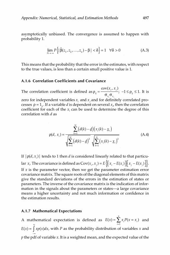
Appendix: Numerical, Statistical, and Estimation Methods 497

asymptotically unbiased. The convergence is assumed to happen with probability 1.

limN→ ∞

P |β(z1, z

2,K, zn ) − β| < δ{ } = 1 ∀δ > 0 (A.3)

This means that the probability that the error in the estimates, with respect to the true values, is less than a certain small positive value is 1.

A.1.6 Correlation Coefficients and Covariance

The correlation coeffi cient is defi ned as ρij =cov(xi , xj )

σxiσxj

; −1 ≤ ρij ≤ 1. It is

zero for independent variables xi and xj and for defi nitely correlated pro-cesses ρ = 1ij . If a variable d is dependent on several xi , then the correlation coeffi cient for each of the xi can be used to determine the degree of this correlation with d as

ρ(d, xi ) =d(k) − d( ) xi (k) − xi( )

k=1

N

∑

d(k) − d( )2

k=1

N

∑ xi (k) − xi( )2

k=1

N

∑ (A.4)

If |ρ(d, xi )| tends to 1 then d is considered linearly related to that particu-

lar xi . The covariance is defi ned as Cov(xi , xj ) = E xi − E(xi )⎡⎣ ⎤⎦ xj − E(xj )⎡⎣ ⎤⎦{ }.

If x is the parameter vector, then we get the parameter estimation error covariance matrix. The square roots of the diagonal elements of this matrix give the standard deviations of the errors in the estimation of states or parameters. The inverse of the covariance matrix is the indication of infor-mation in the signals about the parameters or states—a large covariance means a higher uncertainty and not much information or confi dence in the estimation results.

A.1.7 Mathematical Expectations

A mathematical expectation is defi ned as E(x) = xiP(x = xi )i=1

n

∑ and

E(x) = x−∞

∞

∫ p(x)dx, with P as the probability distribution of variables x and

p the pdf of variable x . It is a weighted mean, and the expected value of the

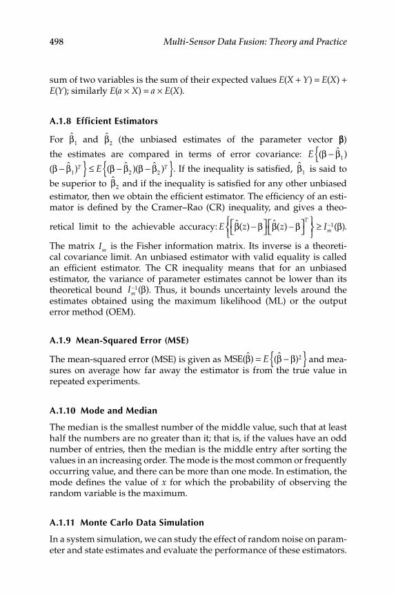
498 Multi-Sensor Data Fusion: Theory and Practice

sum of two variables is the sum of their expected values E ( X + Y ) = E ( X ) + E ( Y ); similarly E ( a × X ) = a × E ( X ).

A.1.8 Efficient Estimator s

For β1 and β

2 (the unbiased estimates of the parameter vector β)

the estimates are compared in terms of error covariance: E (β − β1){

(β − β1)T } ≤ E (β − β

2)(β − β

2)T{ }. If the inequality is satisfi ed, β

1 is said to

be superior to β2 and if the inequality is satisfi ed for any other unbiased

estimator, then we obtain the effi cient estimator. The effi ciency of an esti-mator is defi ned by the Cramer–Rao (CR) inequality, and gives a theo-

retical limit to the achievable accuracy: E β(z) − β⎡

⎣⎤⎦ β(z) − β⎡

⎣⎤⎦

T⎧⎨⎩

⎫⎬⎭

≥ Im−1(β).

The matrix Im is the Fisher information matrix. Its inverse is a theoreti-cal covariance limit. An unbiased estimator with valid equality is called an effi cient estimator. The CR inequality means that for an unbiased estimator, the variance of parameter estimates cannot be lower than its theoretical bound Im

−1(β). Thus, it bounds uncertainty levels around the estimates obtained using the maximum likelihood (ML) or the output error method (OEM).

A.1.9 Mean-Squared Error (MSE)

The mean-squared error (MSE) is given as MSE(β) = E (β − β)2{ } and mea-sures on average how far away the estimator is from the true value in repeated experiments.

A.1.10 Mode and Median

The median is the smallest number of the middle value, such that at least half the numbers are no greater than it; that is, if the values have an odd number of entries, then the median is the middle entry after sorting the values in an increasing order. The mode is the most common or frequently occurring value, and there can be more than one mode. In estimation, the mode defi nes the value of x for which the probability of observing the random variable is the maximum.

A.1.11 Monte Carlo Data Simulation

In a system simulation, we can study the effect of random noise on param-eter and state estimates and evaluate the performance of these estimators.

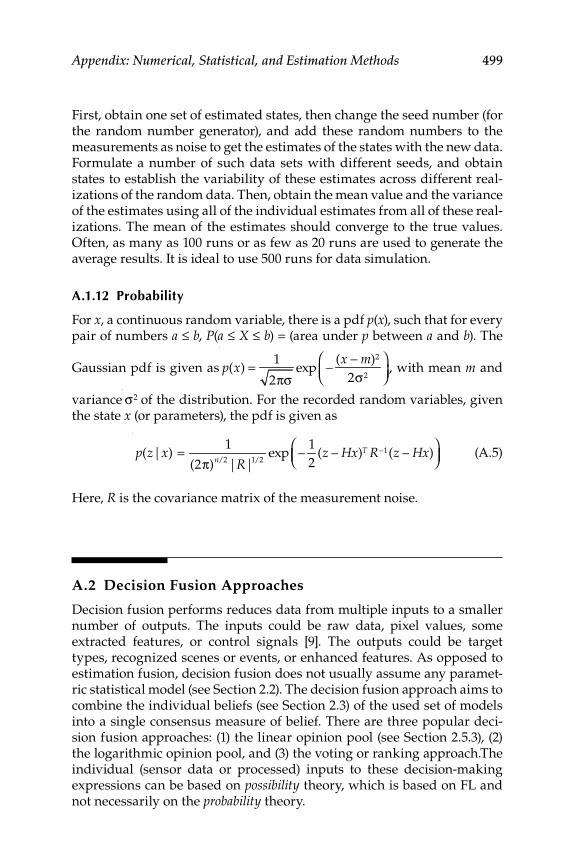
Appendix: Numerical, Statistical, and Estimation Methods 499

First, obtain one set of estimated states, then change the seed number (for the random number generator), and add these random numbers to the measurements as noise to get the estimates of the states with the new data. Formulate a number of such data sets with different seeds, and obtain states to establish the variability of these estimates across different real-izations of the random data. Then, obtain the mean value and the variance of the estimates using all of the individual estimates from all of these real-izations. The mean of the estimates should converge to the true values. Often, as many as 100 runs or as few as 20 runs are used to generate the average results. It is ideal to use 500 runs for data simulation.

A.1.12 Probability

For x , a continuous random variable, there is a pdf p ( x ), such that for every pair of numbers a ≤ b , P ( a ≤ X ≤ b ) = (area under p between a and b ). The

Gaussian pdf is given as

p(x) = 1

2πσexp − (x − m)2

2σ2

⎛⎝⎜

⎞⎠⎟, with mean m and

variance σ2 of the distribution. For the recorded random variables, given the state x (or parameters), the pdf is given as

p(z|x) = 1

(2π)n/2|R|1/2exp –

1

2(z – Hx)T R−1(z – Hx)

⎛⎝⎜

⎞⎠⎟

(A.5)

Here, R is the covariance matrix of the measurement noise.

A.2 Decision Fusion Approaches

Decision fusion performs reduces data from multiple inputs to a smaller number of outputs. The inputs could be raw data, pixel values, some extracted features, or control signals [9]. The outputs could be target types, recognized scenes or events, or enhanced features. As opposed to estimation fusion, decision fusion does not usually assume any paramet-ric statistical model (see Section 2.2). The decision fusion approach aims to combine the individual beliefs (see Section 2.3) of the used set of models into a single consensus measure of belief. There are three popular deci-sion fusion approaches: (1) the linear opinion pool (see Section 2.5.3), (2) the logarithmic opinion pool, and (3) the voting or ranking approach.The individual (sensor data or processed) inputs to these decision-making expressions can be based on possibility theory, which is based on FL and not necessarily on the probability theory.

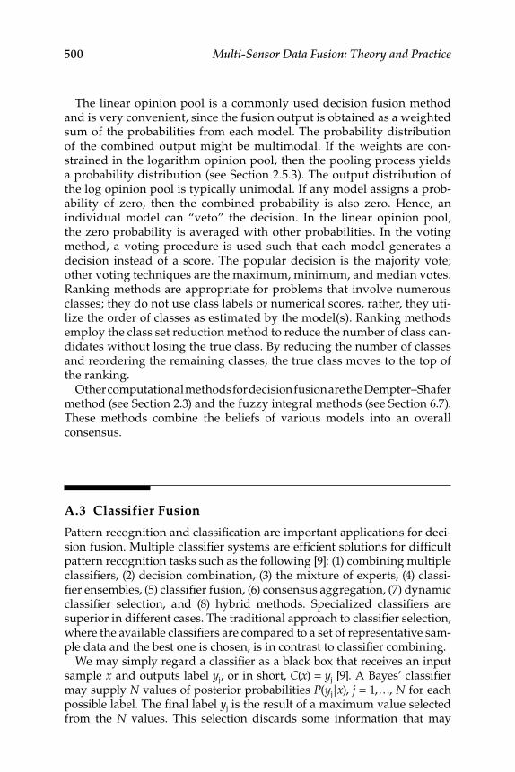
500 Multi-Sensor Data Fusion: Theory and Practice

The linear opinion pool is a commonly used decision fusion method and is very convenient, since the fusion output is obtained as a weighted sum of the probabilities from each model. The probability distribution of the combined output might be multimodal. If the weights are con-strained in the logarithm opinion pool, then the pooling process yields a probability distribution (see Section 2.5.3). The output distribution of the log opinion pool is typically unimodal. If any model assigns a prob-ability of zero, then the combined probability is also zero. Hence, an individual model can “veto” the decision. In the linear opinion pool, the zero probability is averaged with other probabilities. In the voting method, a voting procedure is used such that each model generates a decision instead of a score. The popular decision is the majority vote; other voting techniques are the maximum, minimum, and median votes. Ranking methods are appropriate for problems that involve numerous classes; they do not use class labels or numerical scores, rather, they uti-lize the order of classes as estimated by the model(s). Ranking methods employ the class set reduction method to reduce the number of class can-didates without losing the true class. By reducing the number of classes and reordering the remaining classes, the true class moves to the top of the ranking.

Other computational methods for decision fusion are the Dempter–Shafer method (see Section 2.3) and the fuzzy integral methods (see Section 6.7). These methods combine the beliefs of various models into an overall consensus.

A.3 Classifier Fusion

P attern recognition and classifi cation are important applications for deci-sion fusion. Multiple classifi er systems are effi cient solutions for diffi cult pattern recognition tasks such as the following [9]: (1) combining multiple classifi ers, (2) decision combination, (3) the mixture of experts, (4) classi-fi er ensembles, (5) classifi er fusion, (6) consensus aggregation, (7) dynamic classifi er selection, and (8) hybrid methods. Specialized classifi ers are superior in different cases. The traditional approach to classifi er selection, where the available classifi ers are compared to a set of representative sam-ple data and the best one is chosen, is in contrast to classifi er combining.

We may simply regard a classifi er as a black box that receives an input sample x and outputs label y j , or in short, C ( x ) = y j [9]. A Bayes’ classifi er may supply N values of posterior probabilities P ( y j | x ), j = 1,…, N for each possible label. The fi nal label y j is the result of a maximum value selected from the N values. This selection discards some information that may

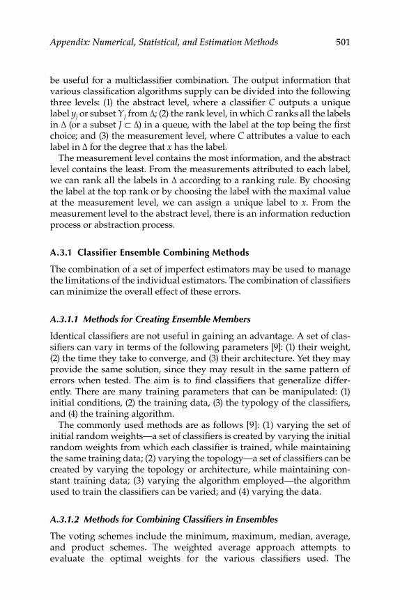
Appendix: Numerical, Statistical, and Estimation Methods 501

be useful for a multiclassifi er combination. The output information that various classifi cation algorithms supply can be divided into the following three levels: (1) the abstract level, where a classifi er C outputs a unique label y j or subset Y J from Δ; (2) the rank level, in which C ranks all the labels in Δ (or a subset J ⊂ Δ) in a queue, with the label at the top being the fi rst choice; and (3) the measurement level, where C attributes a value to each label in Δ for the degree that x has the label.

The measurement level contains the most information, and the abstract level contains the least. From the measurements attributed to each label, we can rank all the labels in Δ according to a ranking rule. By choosing the label at the top rank or by choosing the label with the maximal value at the measurement level, we can assign a unique label to x . From the measurement level to the abstract level, there is an information reduction process or abstraction process.

A.3.1 Classifier Ensemble Combining Methods

The combination of a set of imperfect estimators may be used to manage the limitations of the individual estimators. The combination of classifi ers can minimize the overall effect of these errors.

A.3.1.1 Methods for Creating Ensemble Members

Identical classifi ers are not useful in gaining an advantage. A set of clas-sifi ers can vary in terms of the following parameters [9]: (1) their weight, (2) the time they take to converge, and (3) their architecture. Yet they may provide the same solution, since they may result in the same pattern of errors when tested. The aim is to fi nd classifi ers that generalize differ-ently. There are many training parameters that can be manipulated: (1) initial conditions, (2) the training data, (3) the typology of the classifi ers, and (4) the training algorithm.

The commonly used methods are as follows [9]: (1) varying the set of initial random weights—a set of classifi ers is created by varying the initial random weights from which each classifi er is trained, while maintaining the same training data; (2) varying the topology—a set of classifi ers can be created by varying the topology or architecture, while maintaining con-stant training data; (3) varying the algorithm employed—the algorithm used to train the classifi ers can be varied; and (4) varying the data.

A.3.1.2 Methods for Combining Classifi ers in Ensembles

The voting schemes include the minimum, maximum, median, average, and product schemes. The weighted average approach attempts to evaluate the optimal weights for the various classifi ers used. The

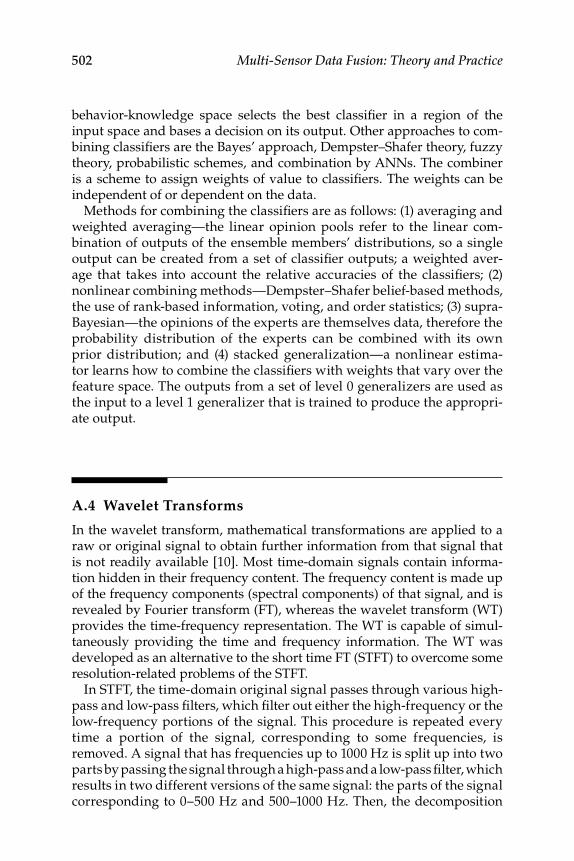
502 Multi-Sensor Data Fusion: Theory and Practice

behavior- knowledge space selects the best classifi er in a region of the input space and bases a decision on its output. Other approaches to com-bining classifi ers are the Bayes’ approach, Dempster–Shafer theory, fuzzy theory, probabilistic schemes, and combination by ANNs. The combiner is a scheme to assign weights of value to classifi ers. The weights can be independent of or dependent on the data.

Methods for combining the classifi ers are as follows: (1) averaging and weighted averaging—the linear opinion pools refer to the linear com-bination of outputs of the ensemble members’ distributions, so a single output can be created from a set of classifi er outputs; a weighted aver-age that takes into account the relative accuracies of the classifi ers; (2) nonlinear combining methods—Dempster–Shafer belief-based methods, the use of rank-based information, voting, and order statistics; (3) supra-Bayesian—the opinions of the experts are themselves data, therefore the probability distribution of the experts can be combined with its own prior distribution; and (4) stacked generalization—a nonlinear estima-tor learns how to combine the classifi ers with weights that vary over the feature space. The outputs from a set of level 0 generalizers are used as the input to a level 1 generalizer that is trained to produce the appropri-ate output.

A.4 Wavelet Transforms

In the wavelet transform, mathematical transformations are applied to a raw or original signal to obtain further information from that signal that is not readily available [10]. Most time-domain signals contain informa-tion hidden in their frequency content. The frequency content is made up of the frequency components (spectral components) of that signal, and is revealed by Fourier transform (FT), whereas the wavelet transform (WT) provides the time-frequency representation. The WT is capable of simul-taneously providing the time and frequency information. The WT was developed as an alternative to the short time FT (STFT) to overcome some resolution-related problems of the STFT.

In STFT, the time-domain original signal passes through various high-pass and low-pass fi lters, which fi lter out either the high-frequency or the low-frequency portions of the signal. This procedure is repeated every time a portion of the signal, corresponding to some frequencies, is removed. A signal that has frequencies up to 1000 Hz is split up into two parts by passing the signal through a high-pass and a low-pass fi lter, which results in two different versions of the same signal: the parts of the signal corresponding to 0–500 Hz and 500–1000 Hz. Then, the decomposition

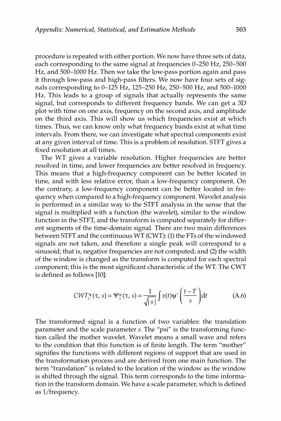
Appendix: Numerical, Statistical, and Estimation Methods 503

procedure is repeated with either portion. We now have three sets of data, each corresponding to the same signal at frequencies 0–250 Hz, 250–500 Hz, and 500–1000 Hz. Then we take the low-pass portion again and pass it through low-pass and high-pass fi lters. We now have four sets of sig-nals corresponding to 0–125 Hz, 125–250 Hz, 250–500 Hz, and 500–1000 Hz. This leads to a group of signals that actually represents the same signal, but corresponds to different frequency bands. We can get a 3D plot with time on one axis, frequency on the second axis, and amplitude on the third axis. This will show us which frequencies exist at which times. Thus, we can know only what frequency bands exist at what time intervals. From there, we can investigate what spectral components exist at any given interval of time. This is a problem of resolution. STFT gives a fi xed resolution at all times.

The WT gives a variable resolution. Higher frequencies are better resolved in time, and lower frequencies are better resolved in frequency. This means that a high-frequency component can be better located in time, and with less relative error, than a low-frequency component. On the contrary, a low-frequency component can be better located in fre-quency when compared to a high-frequency component. Wavelet analysis is performed in a similar way to the STFT analysis in the sense that the signal is multiplied with a function (the wavelet), similar to the window function in the STFT, and the transform is computed separately for differ-ent segments of the time-domain signal. There are two main differences between STFT and the continuous WT (CWT): (1) the FTs of the windowed signals are not taken, and therefore a single peak will correspond to a sinusoid; that is, negative frequencies are not computed; and (2) the width of the window is changed as the transform is computed for each spectral component; this is the most signifi cant characteristic of the WT. The CWT is defi ned as follows [10] :

CWTxψ (τ, s) = Ψx

ψ (τ, s) = 1

|s|x(t)ψ *

t − Ts

⎛⎝⎜

⎞⎠⎟

dt∫ (A.6)

The transformed signal is a function of two variables: the translation parameter and the scale parameter s . The “psi” is the transforming func-tion called the mother wavelet. Wavelet means a small wave and refers to the condition that this function is of fi nite length. The term “mother” signifi es the functions with different regions of support that are used in the transformation process and are derived from one main function. The term “translation” is related to the location of the window as the window is shifted through the signal. This term corresponds to the time informa-tion in the transform domain. We have a scale parameter, which is defi ned as 1/frequency.

504 Multi-Sensor Data Fusion: Theory and Practice

A.5 Type-2 Fuzzy Logic

Type-2 FL handles uncertainties by modeling them and minimizing their effects [11]. If all uncertainties disappear, Type-2 FL is reduced to Type-1 FL. A rule-based FL system (FLS) consists of a fuzzifi er, an infer-ence mechanism or engine (fuzzy inference system [FIS] associated with the specifi ed rules), an output processor ([o/p]; fuzzy implication method [FIM] for operations on fuzzy sets that are characterized by membership functions), and the defuzzifi cation process. The o/p for a Type-1 FLS is a defuzzifi er, and it transforms a Type-1 fuzzy set into a Type-0 fuzzy set. The o/p for a Type-2 FLS has two components: (1) Type-2 fuzzy sets are transformed into Type-1 fuzzy sets by means of type reduction; and (2) the type-reduced set is then transformed into a number by means of defuzz-ifcation. Type-1 FLS does not directly handle rule uncertainties because it uses Type-1 fuzzy sets that are certain. Type-2 FLS is very useful in circumstances in which it is diffi cult to determine an exact membership function for a fuzzy set. They can be used to handle rule uncertainties and even measurement uncertainties.

The output of a Type-1 FLS (the defuzzifi ed output) is analogous to the mean of a pdf. In probability theory, the variance provides a measure of dispersion about the mean and captures more information about the prob-abilistic uncertainty. Type-2 FL provides this measure of dispersion, which is fundamental to the design of systems that include linguistic or numeri-cal uncertainties that translate into rule or input uncertainties. Linguistic and random uncertainties “fl ow” through a Type-2 FLS. These effects can be evaluated using the defuzzifi ed output and the type-reduced output of that system. The type-reduced output provides a measure of disper-sion about the defuzzifi ed output and can be thought of as related to a linguistic confi dence interval. The type-reduced set increases as linguistic or random uncertainties increase; hence a Type-2 FLS is analogous to a probabilistic system (via fi rst and second moments), whereas a Type-1 FLS is analogous to a probabilistic system only through the fi rst moment, the mean.

A Type-2 FLS has more design DOF than a Type-1 FLS. This is because Type-2 fuzzy sets are described by more parameters than are Type-1 fuzzy sets; this signifi es that a Type-2 FLS can have better performance than a Type-1 FLS. Although there is no mathematical proof that this will always be the case, in every application of Type-2 FLS, a better perfor-mance has been obtained using a Type-2 FLS than is obtained using a Type-1 FLS [11]. Thus, Type-2 FLS is required to directly model uncertain-ties and minimize their effects within the framework of rule-based FLSs. This can also be extended to MSDF and other decision fusion approaches based on FL.

Appendix: Numerical, Statistical, and Estimation Methods 505

A.6 Neural Networks

Biological neural networks (BNNs) and ANNs have the ability to continue functioning with noisy and/or incomplete information, have robustness or fault tolerance, and can adapt to changing environments by learning [1]. ANNs attempt to mimic and exploit the parallel-processing capability of the human brain. ANNs are modeled based on the parallel biological structures found in the brain and thus simulate a highly interconnected parallel computational structure with relatively simple individual pro-cessing elements called neurons. The human brain has between 10 and 500 billion neurons and approximately 1000 main modules with 500 neural networks (NWs). Each neural NW has 100,000 neurons [5–7]. The neuron is the fundamental building block of the nervous system. A comparison of BNNs and ANNs is given in Table A.1.

Conventional computers cannot match the human brain’s capacity for several tasks: (1) speech processing, (2) image processing, (3) pattern rec-ognition, and (4) heuristic reasoning and universal problem solving. Each biological neuron is connected to approximately 10,000 other neurons, giv-ing it a massively parallel computing capability. The brain solves certain problems with two main characteristics: (1) problems that are ill-defi ned; and (2) problems that require a very large amount of processing. Hence, the similarity between BNNs and ANNs is that each system typically con-sists of a large number of simple elements that learn and are collectively able to solve complicated problems. ANNs have been successfully applied in image processing, pattern recognition, nonlinear curve fi tting or map-ping, aerodynamic modeling, fl ight data analysis, adaptive control, system

TABLE A.1

A Comparison of Biological and Artifi cial Neuronal Systems

ANN System BNN System

The signals or data enter the input layer Dendrites are the input branches and

connect to a set of other neurons

The hidden layer is between the input and

output layers

The soma is the cell body wherein all the

logical functions of the neurons are

performed

The output layer produces the NW’s output

responses, linear or nonlinear

The axon nerve fi ber is the output channel;

the signals are converted into nerve

pulses (spikes) to target cells

Weights and coeffi cients are the strength of

the connection between nodes

Synapses are the contacts on a neuron; they

interface some axons to the spines of the

input dendrites, and can enhance or

dampen the neuronal excitation

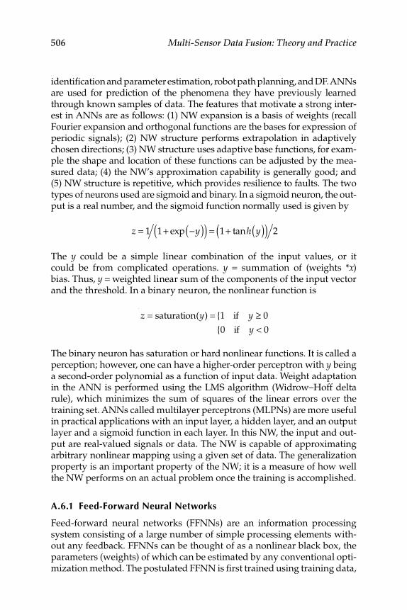
506 Multi-Sensor Data Fusion: Theory and Practice

identifi cation and parameter estimation, robot path planning, and DF. ANNs are used for prediction of the phenomena they have previously learned through known samples of data. The features that motivate a strong inter-est in ANNs are as follows: (1) NW expansion is a basis of weights (recall Fourier expansion and orthogonal functions are the bases for expression of periodic signals); (2) NW structure performs extrapolation in adaptively chosen directions; (3) NW structure uses adaptive base functions, for exam-ple the shape and location of these functions can be adjusted by the mea-sured data; (4) the NW’s approximation capability is generally good; and (5) NW structure is repetitive, which provides resilience to faults. The two types of neurons used are sigmoid and binary. In a sigmoid neuron, the out-put is a real number, and the sigmoid function normally used is given by

z = 1 1+ exp −y( )( ) = 1+ tanh y( )( ) 2

The y could be a simple linear combination of the input values, or it could be from complicated operations. y = summation of (weights * x ) bias. Thus, y = weighted linear sum of the components of the input vector and the threshold. In a binary neuron, the nonlinear function is

z = saturation(y) = {1 if y ≥ 0

{0 if y < 0

The binary neuron has saturation or hard nonlinear functions. It is called a perception; however, one can have a higher-order perceptron with y being a second-order polynomial as a function of input data. Weight adaptation in the ANN is performed using the LMS algorithm (Widrow–Hoff delta rule), which minimizes the sum of squares of the linear errors over the training set. ANNs called multilayer perceptrons (MLPNs) are more useful in practical applications with an input layer, a hidden layer, and an output layer and a sigmoid function in each layer. In this NW, the input and out-put are real-valued signals or data. The NW is capable of approximating arbitrary nonlinear mapping using a given set of data. The generalization property is an important property of the NW; it is a measure of how well the NW performs on an actual problem once the training is accomplished.

A.6.1 Feed-Forward Neural Networks

Feed-forward neural networks (FFNNs) are an information processing system consisting of a large number of simple processing elements with-out any feedback. FFNNs can be thought of as a nonlinear black box, the parameters (weights) of which can be estimated by any conventional opti-mization method. The postulated FFNN is fi rst trained using training data,

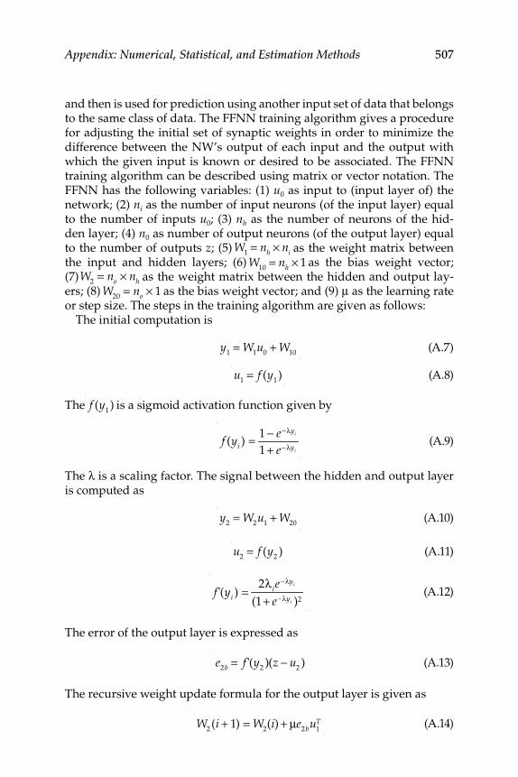
Appendix: Numerical, Statistical, and Estimation Methods 507

and then is used for prediction using another input set of data that belongs to the same class of data. The FFNN training algorithm gives a procedure for adjusting the initial set of synaptic weights in order to minimize the difference between the NW’s output of each input and the output with which the given input is known or desired to be associated. The FFNN training algorithm can be described using matrix or vector notation. The FFNN has the following variables: (1) u0 as input to (input layer of) the network; (2) ni as the number of input neurons (of the input layer) equal to the number of inputs u0; (3) nh as the number of neurons of the hid-den layer; (4) n0 as number of output neurons (of the output layer) equal to the number of outputs z ; (5) W

1= nh × ni as the weight matrix between

the input and hidden layers; (6) W10

= nh × 1 as the bias weight vector; (7)W

2= no × nh as the weight matrix between the hidden and output lay-

ers; (8) W20

= no × 1 as the bias weight vector; and (9) μ as the learning rate or step size. The steps in the training algorithm are given as follows:

The initial computation is

y

1= W

1u

0+ W

10 (A.7)

u1

= f (y1) (A.8)

The f (y

1) is a sigmoid activation function given by

f (yi ) =

1 − e−λyi

1 + e−λyi

(A.9)

The λ is a scaling factor. The signal between the hidden and output layer is computed as

y

2= W

2u

1+ W

20 (A.10)

u2

= f (y2) (A.11)

f '(yi ) =

2λ ie−λyi

(1+ e−λyi )2 (A.12)

The error of the output layer is expressed as

e

2b = f '(y2)(z − u

2) (A.13)

The recursive weight update formula for the output layer is given as

W

2(i + 1) = W

2(i) + μe

2bu1T (A.14)

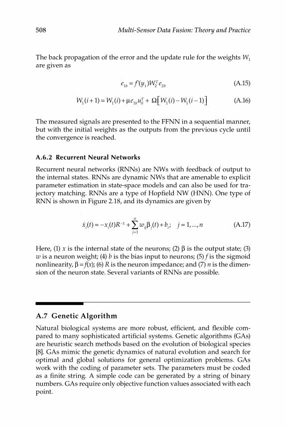
508 Multi-Sensor Data Fusion: Theory and Practice

The back propagation of the error and the update rule for the weights W1 are given as

e

1b = f '(y1)W

2T e

2b (A.15)

W

1(i + 1) = W

1(i) + μe

1bu0T + Ω W

1(i) − W

1(i − 1)⎡⎣ ⎤⎦ (A.16)

The measured signals are presented to the FFNN in a sequential manner, but with the initial weights as the outputs from the previous cycle until the convergence is reached.

A.6.2 Recurrent Neural Networks

Recurrent neural networks (RNNs) are NWs with feedback of output to the internal states. RNNs are dynamic NWs that are amenable to explicit parameter estimation in state-space models and can also be used for tra-jectory matching. RNNs are a type of Hopfi eld NW (HNN). One type of RNN is shown in Figure 2.18, and its dynamics are given by

&xi(t) = −xi(t)R−1 + wijβ j(t) + bi

j=1

n

∑ ; j = 1,..., n (A.17)

Here, (1) x is the internal state of the neurons; (2) β is the output state; (3) w is a neuron weight; (4) b is the bias input to neurons; (5) f is the sigmoid nonlinearity, β = f ( x ); (6) R is the neuron impedance; and (7) n is the dimen-sion of the neuron state. Several variants of RNNs are possible.

A.7 Genetic Algorithm

Natural biological systems are more robust, effi cient, and fl exible com-pared to many sophisticated artifi cial systems. Genetic algorithms (GAs) are heuristic search methods based on the evolution of biological species [8]. GAs mimic the genetic dynamics of natural evolution and search for optimal and global solutions for general optimization problems. GAs work with the coding of parameter sets. The parameters must be coded as a fi nite string. A simple code can be generated by a string of binary numbers. GAs require only objective function values associated with each point.

Appendix: Numerical, Statistical, and Estimation Methods 509

A.7.1 Chromosomes, Populations, and Fitness

A chromosome is a string constructed by the encoding of information. The GA operates on a number of such chromosomes. A collection of chro-mosomes is a population. Each chromosome consists of a string of bits. Each bit is a binary 0 or 1, or it may be a symbol from a set of more than two elements. Each member is called an individual and is assigned a fi t-ness value based on the objective function.

A.7.2 Reproduction, Crossover, Mutation, and Generation

In reproduction, chromosomes are copied so that the individuals with a higher fi tness have a higher number of copies compared with other indi-viduals. In crossover, members of the newly reproduced strings in the pool are mated at random. Each chromosome is split at a crossover site, selected randomly, and then new chromosomes are formed by joining the top piece of one chromosome with the tail of another. Mutation involves a random change of the value of a string position. The GA consists of a number of such generations of the above operations. In each genera-tion, pairs of individual chromosomes cross over, mutation is randomly applied during the crossover operation, and the new chromosomes that evolve from these operations are placed at a relevant ranked place in the population according to their fi tness. The fi ttest individuals replace the weakest individuals from the previous generation. Thus, a fi tter popula-tion evolves. For real numbers, the crossover can be performed using the average of the two chromosomes.

A.8 System Identification and Parameter Estimation

D ynamic systems can generally be described by a set of difference or differential equations. Such equations are formulated in the state space, which has a nice matrix structure. Therefore, the dynamics of the systems can be represented fairly well by linear or nonlinear state-space equations. Then, the problem of parameter estimation pertains to the determination of the numerical values of these matrices’ elements, which form the struc-ture of the state-space equations [1]. In the system identifi cation problem, the coeffi cients of transfer function (numerator polynomial or denomina-tor polynomial) are determined from the input–output data of the system using optimization procedures [2–4]. Parameter estimation is an impor-tant aspect in model building using the empirical data of the system.

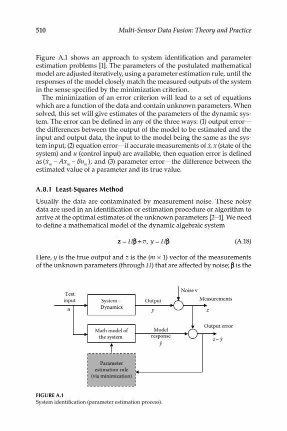
510 Multi-Sensor Data Fusion: Theory and Practice

Figure A.1 shows an approach to system identifi cation and parameter estimation problems [1]. The parameters of the postulated mathematical model are adjusted iteratively, using a parameter estimation rule, until the responses of the model closely match the measured outputs of the system in the sense specifi ed by the minimization criterion.

The minimization of an error criterion will lead to a set of equations which are a function of the data and contain unknown parameters. When solved, this set will give estimates of the parameters of the dynamic sys-tem. The error can be defi ned in any of the three ways: (1) output error—the differences between the output of the model to be estimated and the input and output data, the input to the model being the same as the sys-tem input; (2) equation error—if accurate measurements of x, x (state of the system) and u (control input) are available, then equation error is defi ned as ( &xm − Axm − Bum ); and (3) parameter error—the difference between the estimated value of a parameter and its true value.

A.8.1 Least-Squares Method

Usually the data are contaminated by measurement noise. These noisy data are used in an identifi cation or estimation procedure or algorithm to arrive at the optimal estimates of the unknown parameters [2–4]. We need to defi ne a mathematical model of the dynamic algebraic system

z = Hβ + v, y = Hβ (A.18)

Here, y is the true output and z is the ( m × 1) vector of the measurements of the unknown parameters (through H ) that are affected by noise; β is the

FIGURE A.1 System identifi cation (parameter estimation process).

System - Dynamics

Noise v

Output Measurements

Output errorModel

response

Testinput

Math model ofthe system

Parameterestimation rule

(via minimization)

u y z

z −y

yˆ

ˆ

Appendix: Numerical, Statistical, and Estimation Methods 511

( n × 1) vector of the unknown parameters; and v is the measurement noise or errors. The noise is assumed to be zero mean, white, and Gaussian. In general, least-squares (LS) method is applicable to linear and nonlinear problems. The LS estimate of β is given as

βLS = (HT H)−1 HT z (A.19)

Some properties of the LS estimates are as follows: (1) βLS is a linear func-tion of the data vector z . H could contain input or output data of the system; (2) the error in the estimator is a linear function of the measure-ment errors (vk ); (3) if the measurement errors are large, then the error in estimation is large; (4) if E { v } is zero, then the LS estimate is unbiased; and (5) the covariance of the estimation error is given as

E %βLS

%βLST{ } ≅ P = (HT H)−1 HT RH(HT H)−1

(A.20)

Here, R is the covariance matrix of v . If v is uncorrelated and its compo-

nents have identical variances, then R = σ2I, where I is an identity matrix. Thus, we have

cov %βLS( ) = P = σ2(HT H)−1 (A.21)

Hence, the standard deviation of the parameter estimates can be obtained

as Pii , ignoring the effect of cross terms of the matrix P . The use of a weighting matrix W in the LS criterion function gives the cost function for the Gaussian LS (GLS) method

J = (z − Hβ)T W(z − Hβ) (A.22)

W is the symmetric and positive defi nite and is used to control the infl u-ence of specifi c measurements upon the estimates of β. The solution exists if the weighting matrix is positive defi nite.

A.8.2 Maximum Likelihood and Output Error Methods

The ML method invokes the probabilistic aspect of random variables (e.g., measurements or errors) and uses a process which obtains estimates of the parameters [1]. These parameters are most likely to produce model responses that closely match the measurements. An LF, akin to the pdf, is defi ned when the measurements are collected and used in the pdf. The LF is maximized to obtain the ML estimates of the parameters of the dynamic system. The OEM is an ML estimator (MLE) for data containing only mea-surement noise. The Gaussian LS (GLS) differential correction method is

512 Multi-Sensor Data Fusion: Theory and Practice

also an OEM, but it is not based on the ML principle. In any estimator, the error is made in the estimates relative to the true values of the parameters. The true parameters are unknown in any real case. We get only a few sta-tistical indicators for the errors made. The Cramer–Rao (CR) lower bound is one such useful measure for these errors. For unbiased and effi cient estimators, the CR lower bound is given as

σβe

2 = Im−1(β)

The inverse of the information matrix is the covariance matrix. The infor-mation matrix can be computed from the LF or related data. The CR lower bound signifi es that the variance in the estimator for an effi cient estimator will be at least equal to the predicted variance, whereas for other cases, it could be greater but not less than the predicted value. Thus, the pre-dicted value provides the lower bound. Let a linear dynamical system be described as

&x(t) = Ax(t)+ Bu(t) (A.23)

y(t) = Hx(t) (A.24)

z(k) = y(k)+ v(k) (A.25)

The following assumptions are made regarding the measurement noise v(k) :

E{v(k)} = 0; E{v(k)vT(l)} = Rδkl (A.26)

In Equation A.26, we assume that the measurement noise is zero mean and white Gaussian with R as the covariance matrix of this noise. This assumption allows us to use the Gaussian probability concept for deriving the MLE. The parameter vector β is obtained by maximizing the LF with respect to β by minimizing the negative (log) LF:

L = − log p(z|β, R) = 1

2z(k)− y(k)⎡⎣ ⎤⎦

TR−1 z(k)− y(k)⎡⎣ ⎤⎦

k=1

N

∑

+ N2

log|R|+ const (A.27)

Minimization of L w.r.t. β (under not too restrictive conditions) results in

∂L∂β= −

∂y(β)

∂β⎛⎝⎜

⎞⎠⎟

T

R−1 z − y(β)( )k∑ = 0 (A.28)

This yields a system of nonlinear equations. In the present case, we obtain an iterative solution by using quasi-linearization method (also

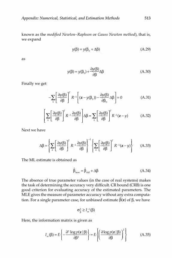
Appendix: Numerical, Statistical, and Estimation Methods 513

known as the modifi ed Newton–Raphson or Gauss Newton method ), that is, we expand

y(β) = y(β

0+ Δβ) (A.29)

as

y(β) = y(β

0)+∂y(β)

∂βΔβ (A.30)

Finally we get

−∂y(β)

∂β⎡

⎣⎢

⎤

⎦⎥

T

R−1 (z − y(β0))−

∂y(β)

∂β0

Δβ⎡

⎣⎢

⎤

⎦⎥ = 0

k∑ (A.31)

∂y(β)

∂β⎡

⎣⎢

⎤

⎦⎥

T

k∑ R−1

∂y(β)

∂β

⎡

⎣⎢⎢

⎤

⎦⎥⎥Δβ =

∂y(β)

∂β⎡

⎣⎢

⎤

⎦⎥

T

k∑ R−1(z − y) (A.32)

Next we have

Δβ =∂y(β)

∂β⎡

⎣⎢

⎤

⎦⎥

T

R−1∂y(β)

∂βk∑⎧⎨⎪

⎩⎪

⎫⎬⎪

⎭⎪

−1

∂y(β)

∂β⎡

⎣⎢

⎤

⎦⎥

T

R−1(z − y)k∑⎧⎨⎪

⎩⎪

⎫⎬⎪

⎭⎪ (A.33)

The ML estimate is obtained as

β

new= β

old+ Δβ (A.34)

The absence of true parameter values (in the case of real systems) makes the task of determining the accuracy very diffi cult. CR bound (CRB) is one good criterion for evaluating accuracy of the estimated parameters. The MLE gives the measure of parameter accuracy without any extra computa-

tion. For a single parameter case, for unbiased estimate β(z) of β , we have

σβ2 ≥ Im

−1(β)

Here, the information matrix is given as

Im(β) = E −∂2 log p(z|β)

∂β2

⎧⎨⎩

⎫⎬⎭= E

∂ log p(z|β)

∂β⎛⎝⎜

⎞⎠⎟

2⎧⎨⎪

⎩⎪

⎫⎬⎪

⎭⎪ (A.35)

514 Multi-Sensor Data Fusion: Theory and Practice

For several parameters, CR inequality is given by

σβi

2 ≥ (Im−1)ii

Here, the information matrix is

(Im )ij = E −∂2 log p(z|β)

∂βi∂β j

⎧⎨⎪

⎩⎪

⎫⎬⎪

⎭⎪=

∂ log p(z|β)

∂βi

⎛⎝⎜

⎞⎠⎟⋅∂ log p(z|β)

∂β j

⎛

⎝⎜

⎞

⎠⎟

⎧⎨⎪

⎩⎪

⎫⎬⎪

⎭⎪ (A.36)

For an effi cient estimation, the equality holds and the covariance matrix of the estimation errors is given by

P = Im

−1

The standard deviation of the parameters is given by

σβi= Pii = P(i, i)

and the correlation coeffi cients are given as

ρβi ,β j=

Pij

PiiPjj (A.37)

For MLE we have

log p(z|β) = − 1

2z(k)− y(k)⎡⎣ ⎤⎦

TR−1 z(k)− y(k)⎡⎣ ⎤⎦

k=1

N

∑ + const (A.38)

The information matrix is obtained as follows: differentiate both sides with respect toβi to get

∂ log p(z|β)

∂βi

⎛⎝⎜

⎞⎠⎟=

∂y∂βi

⎛⎝⎜

⎞⎠⎟

T

k∑ R−1(z − y) (A.39)

Differentiate both sides again with respect toβ j to get

∂2 log p(z|β)

∂βi∂β j

⎛

⎝⎜

⎞

⎠⎟ =

∂2y∂βi∂β j

⎛

⎝⎜

⎞

⎠⎟

T

k∑ R−1(z − y) −

∂y∂βi

⎛⎝⎜

⎞⎠⎟

T

k∑ R−1

∂y∂β j

(A.40)

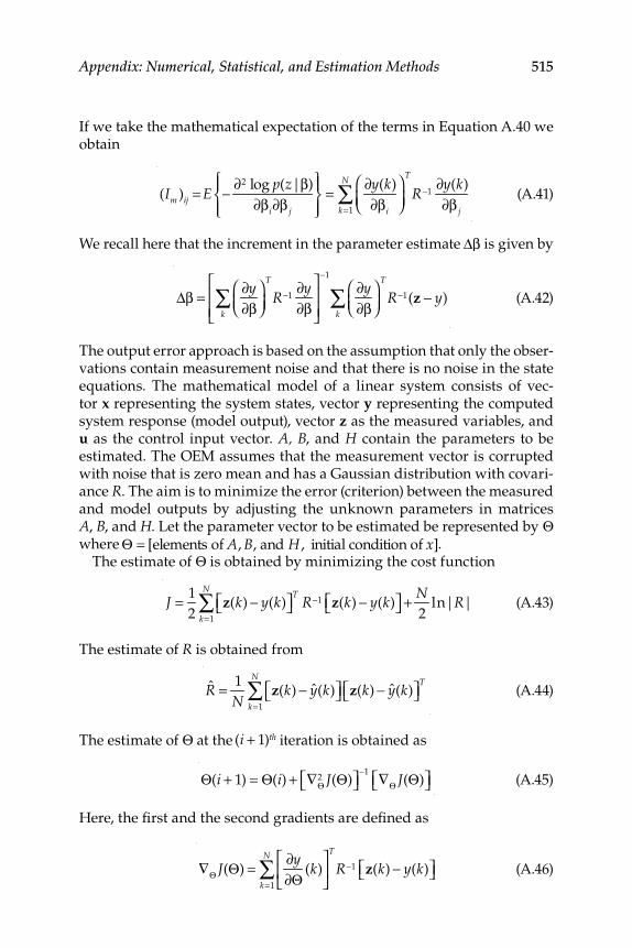
Appendix: Numerical, Statistical, and Estimation Methods 515

If we take the mathematical expectation of the terms in Equation A.40 we obtain

(Im )ij =E −∂2 log p(z|β)

∂βi∂β j

⎧⎨⎪

⎩⎪

⎫⎬⎪

⎭⎪=

∂y(k)

∂βi

⎛⎝⎜

⎞⎠⎟

T

k=1

N

∑ R−1∂y(k)

∂β j

(A.41)

We recall here that the increment in the parameter estimate Δβ is given by

Δβ =∂y∂β⎛⎝⎜

⎞⎠⎟

T

k∑ R−1

∂y∂β

⎡

⎣⎢⎢

⎤

⎦⎥⎥

−1

∂y∂β⎛⎝⎜

⎞⎠⎟

T

R−1

k∑ (z − y) (A.42)

The output error approach is based on the assumption that only the obser-vations contain measurement noise and that there is no noise in the state equations. The mathematical model of a linear system consists of vec-tor x representing the system states, vector y representing the computed system response (model output), vector z as the measured variables, and u as the control input vector. A, B , and H contain the parameters to be estimated. The OEM assumes that the measurement vector is corrupted with noise that is zero mean and has a Gaussian distribution with covari-ance R . The aim is to minimize the error (criterion) between the measured and model outputs by adjusting the unknown parameters in matrices A , B , and H . Let the parameter vector to be estimated be represented by Θ whereΘ = [elements of A, B, and H , initial condition of x].

The estimate of Θ is obtained by minimizing the cost function

J = 1

2z(k)− y(k)⎡⎣ ⎤⎦

TR−1

k=1

N

∑ z(k)− y(k)⎡⎣ ⎤⎦ +N2

ln|R| (A.43)

The estimate of R is obtained from

R = 1

Nz(k)− y(k)⎡⎣ ⎤⎦ z(k)− y(k)⎡⎣ ⎤⎦

T

k=1

N

∑ (A.44)

The estimate of Θ at the (i + 1)th iteration is obtained as

Θ(i + 1) = Θ(i) + ∇Θ

2 J(Θ)⎡⎣ ⎤⎦−1∇Θ J(Θ)⎡⎣ ⎤⎦ (A.45)

Here, the fi rst and the second gradients are defi ned as

∇Θ J(Θ) =

∂y∂Θ

(k)⎡

⎣⎢

⎤

⎦⎥

T

R−1

k=1

N

∑ z(k)− y(k)⎡⎣ ⎤⎦ (A.46)

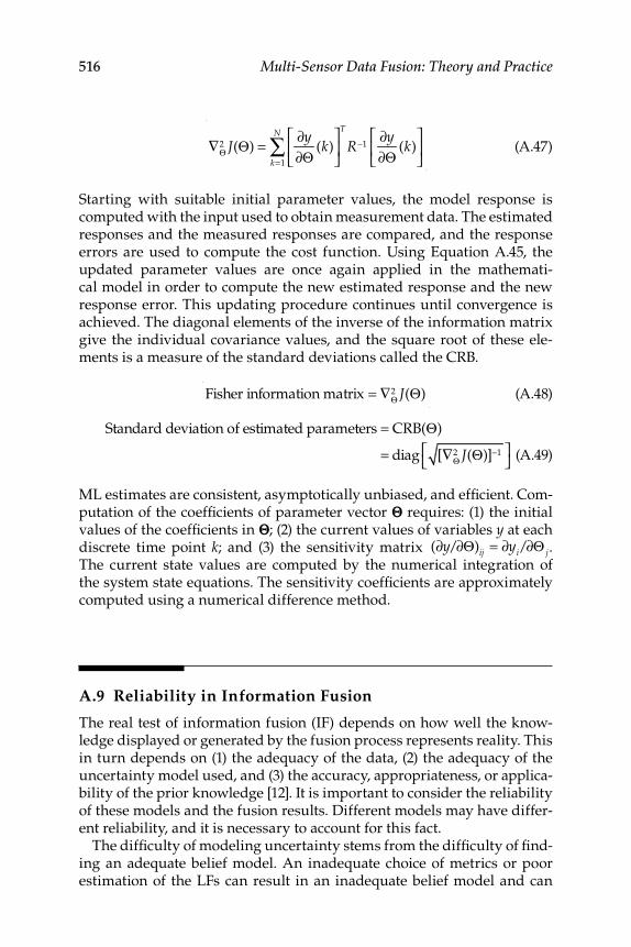
516 Multi-Sensor Data Fusion: Theory and Practice

∇Θ

2 J(Θ) =∂y∂Θ

(k)⎡

⎣⎢

⎤

⎦⎥

T

k=1

N

∑ R−1∂y∂Θ

(k)⎡

⎣⎢

⎤

⎦⎥ (A.47)

Starting with suitable initial parameter values, the model response is computed with the input used to obtain measurement data. The estimated responses and the measured responses are compared, and the response errors are used to compute the cost function. Using Equation A.45, the updated parameter values are once again applied in the mathemati-cal model in order to compute the new estimated response and the new response error. This updating procedure continues until convergence is achieved. The diagonal elements of the inverse of the information matrix give the individual covariance values, and the square root of these ele-ments is a measure of the standard deviations called the CRB.

Fisher information matrix = ∇Θ

2 J(Θ) (A.48)

Standard deviation of estimated parameters = CRB(Θ)

= diag [∇Θ2 J(Θ)]−1⎡

⎣⎤⎦ (A.49)

ML estimates are consistent, asymptotically unbiased, and effi cient. Com-putation of the coeffi cients of parameter vector Θ requires: (1) the initial values of the coeffi cients in Θ; (2) the current values of variables y at each discrete time point k ; and (3) the sensitivity matrix (∂y/∂Θ)ij = ∂yi/∂Θ j. The current state values are computed by the numerical integration of the system state equations. The sensitivity coeffi cients are approximately computed using a numerical difference method.

A.9 Reliability in Information Fusion

The real test of information fusion (IF) depends on how well the know-ledge displayed or generated by the fusion process represents reality. This in turn depends on (1) the adequacy of the data, (2) the adequacy of the uncertainty model used, and (3) the accuracy, appropriateness, or applica-bility of the prior knowledge [12]. It is important to consider the reliability of these models and the fusion results. Different models may have differ-ent reliability, and it is necessary to account for this fact.

The diffi culty of modeling uncertainty stems from the diffi culty of fi nd-ing an adequate belief model. An inadequate choice of metrics or poor estimation of the LFs can result in an inadequate belief model and can

Appendix: Numerical, Statistical, and Estimation Methods 517

lead to a combination of confl icting and unreliable beliefs. Moreover, beliefs can be models within different uncertainty frameworks, and deal-ing with different sources may also mean dealing with different frame-work theories.

Modeling beliefs has always some limitations, and models are only valid within a certain range. Therefore, we have to take into account the range and the limitations of the belief model used for each source when combin-ing information provided by many sources. The most natural way to deal with this problem is to establish the reliability of the beliefs computed within the framework of the model selected. This may be achieved using reliability coeffi cients, which introduce the second level of uncertainty (uncertainty of evaluation of uncertainty) and represent a measure of the adequacy of the model used and the state of the environment observed. There are at least two approaches used for defi ning reliability as a higher-order uncertainty: (1) reliability is understood as the relative stability of the fi rst order uncertainty—reliability is often measured by the perfor-mance of each source (e.g., by recognition or by false alarm rates); and (2) to measure the accuracy of predicted beliefs—reliability coeffi cients represent the adequacy with which each belief model represents the real-ity. In general, fusion operators are based on the assumption that the sources are reliable. If the sources are not reliable, the fusion operators must account for their reliability. This can be represented as F = function of (degree of beliefs, reliability, and coeffi cients). Reliability coeffi cients control how respective sources infl uence fusion results.

The reliability coeffi cient is close to 0 if the source is unreliable and close to 1 if it is more reliable. Reliability coeffi cients depend not only on the model selected but also on the characteristics of the environment and the particular domain of the input. The problem of source reliabil-ity is related to the problem of confl ict. Indeed, the existence of confl ict indicates the existence of at least one unreliable source. Global knowledge about the sources, environment, and the nature and properties of the par-ticular credibility model can provide different information about reliabil-ity. Several situations that differ by the level of knowledge about source reliability can be considered: (1) It is possible to assign a numerical degree of reliability to each source; each value of reliability may be “relative” or “absolute” and may or may not be linked by an equation, such as the sum of reliability coeffi cients being equal to 1; (2) only an order of the reliabili-ties of the sources is known; their precise values are unknown; and (3) a subset of sources is reliable, it is unclear which one in particular is reli-able. Dealing with these situations calls for one or the combination of the following two strategies: (1) explicitly utilizing reliability of the sources; in this case two substrategies may be conceivable: (a) including reliabil-ity before fusion in the modeling belief for each source, to compensate for their different reliability and make them totally, or at least equally,

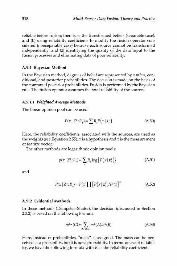
518 Multi-Sensor Data Fusion: Theory and Practice

reliable before fusion; then fuse the transformed beliefs (separable case), and (b) using reliability coeffi cients to modify the fusion operator con-sidered (nonseparable case) because each source cannot be transformed independently; and (2) identifying the quality of the data input to the fusion processes and eliminating data of poor reliability.

A.9.1 Bayesian Method

In the Bayesian method, degrees of belief are represented by a priori , con-ditional, and posterior probabilities. The decision is made on the basis of the computed posterior probabilities. Fusion is performed by the Bayesian rule. The fusion operator assumes the total reliability of the sources.

A.9.1.1 Weighted Average Methods

The linear opinion pool can be used:

P(x|Zk ;Rj ) = RiP x|zi

k( )i∑ (A.50)

Here, the reliability coeffi cients, associated with the sources, are used as the weights (see Equation 2.55). x is a hypothesis and z is the measurement or feature vector.

The other methods are logarithmic opinion pools:

p(x|Zk ;Ri ) = Ri log P x|zik( ){ }

i∑ (A.51)

and

P(x|Zk ;Ri ) = P(x) P x|zi

k( )/P(x){ }Ri

i∏ (A.52)

A.9.2 Evidential Methods

In these methods (Dempster–Shafer), the decision (discussed in Section 2.3.2) is based on the following formula:

m1,2 (C)∝ m1(A)m2 (B)

A∩B=C∑ (A.53)

Here, instead of probabilities, “mass” is assigned. The mass can be per-ceived as a probability, but it is not a probability. In terms of use of reliabil-ity, we have the following formula with R as the reliability coeffi cient.

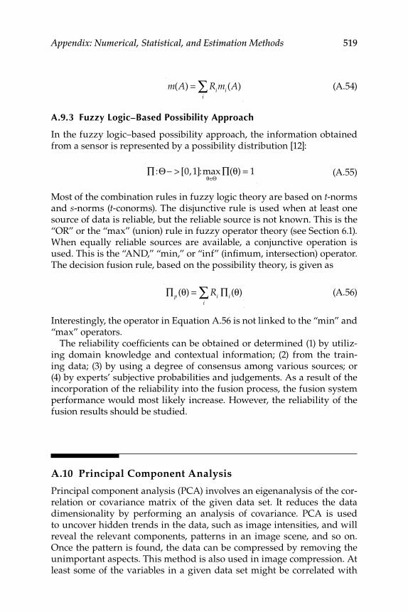
Appendix: Numerical, Statistical, and Estimation Methods 519

m(A) = Rimi

i∑ (A) (A.54)

A.9.3 Fuzzy Logic–Based Possibility Approach

In the fuzzy logic–based possibility approach, the information obtained from a sensor is represented by a possibility distribution [12]:

∏ :Θ− > [0,1]:max

θ∈Θ∏(θ) = 1 (A.55)

Most of the combination rules in fuzzy logic theory are based on t -norms and s -norms ( t -conorms). The disjunctive rule is used when at least one source of data is reliable, but the reliable source is not known. This is the “OR” or the “max” (union) rule in fuzzy operator theory (see Section 6.1). When equally reliable sources are available, a conjunctive operation is used. This is the “AND,” “min,” or “inf” (infi mum, intersection) operator. The decision fusion rule, based on the possibility theory, is given as

∏p (θ) = Ri ∏ i

i∑ (θ) (A.56)

Interestingly, the operator in Equation A.56 is not linked to the “min” and “max” operators.

The reliability coeffi cients can be obtained or determined (1) by utiliz-ing domain knowledge and contextual information; (2) from the train-ing data; (3) by using a degree of consensus among various sources; or (4) by experts’ subjective probabilities and judgements. As a result of the incorporation of the reliability into the fusion process, the fusion system performance would most likely increase. However, the reliability of the fusion results should be studied.

A.10 Principal Component Analysis

Principal component analysis (PCA) involves an eigenanalysis of the cor-relation or covariance matrix of the given data set. It reduces the data dimensionality by performing an analysis of covariance. PCA is used to uncover hidden trends in the data, such as image intensities, and will reveal the relevant components, patterns in an image scene, and so on. Once the pattern is found, the data can be compressed by removing the unimportant aspects. This method is also used in image compression. At least some of the variables in a given data set might be correlated with

520 Multi-Sensor Data Fusion: Theory and Practice

each other, implying some redundancy in the information provided by these variables. PCA exploits the redundancy in such multivariate data and helps detemine the patterns or relationships in the variables. It also reduces the dimensionality of the data set without much loss of information.

A.11 Reliability

Reliability is formally defi ned as the probability that an item will per-form a required function without failure under the stated conditions for a stated period of time. Several other defi nitions of reliability are avail-able in literature on the subject: (1) the ability of equipment, machines, or systems to consistently perform their intended or required function or mission on demand and without degradation or failure; (2) the probability of a failure-free performance over an item’s useful life or a specifi ed time-frame, under specifi ed environmental and duty-cycle conditions, and (3) the consistency and validity of test results determined through statistical methods after repeated trials. Reliability in the context of sensor or DF pertains to reliability of the sensors or data. If the sensors or data are not reliable, then there is no need to fuse these data.

References

1. Raol, J. R., G. Girija, and J. Singh. 2004. Modelling and parameter estimation of dynamic systems, IEE Control Engineering Series Book . Vol. 65. London: IEE (With associated MODEST software in MATLAB via IEE book. NAL web sites).

2. Sorenson, H. W. 1980. Parameter estimation—Principles and problems . New York: Marcel Dekker.

3. Eykhoff, P. 1972. System identifi cation: Parameter and state estimation . London: John Wiley.

4. Ljung, L. 1987. System identifi cation: Theory for the user . Englewood Cliffs, NJ: Prentice Hall.

5. Eerhart, R. C., and R. W. Dobbins. 1993. Neural network PC tools—A practical guide . New York: Academic Press.

6. Hush, D. R., and B. G. Horne. 1993. Progress in supervised neural networks—What is new since Lippmann. IEEE Signal Process Mag 10(1):8–39.

7. King, R. E. 1999. Computational intelligence in control engineering . New York: Marcel Dekker.

Appendix: Numerical, Statistical, and Estimation Methods 521

8. Goldberg, D. E. 1989. Genetic algorithms in search, optimization and machine learning . Boston: Addison-Wesley.

9. Sinha, A., H. Chen, D. G. Danu, T. Kirubarajan, and M. Farooq. 2008. Estimation and decision fusion: A survey. Neurocomputing 71(13–15):2650–6.

10. Polikar, R. From the Fourier transform to the wavelet transform. rowan.du/ ~polikar/WAVELETS/WTutorial.html – 92k (accessed January 2009).

11. Mendel, J. M. 2001. Why we need Type-2 fuzzy logic system. http:// www.informit.com/articles/article.aspx?p=21312-32k. May 2001.

12. Rogova, G. L., and V. Nimier. 2004. Reliability in information fusion. In Proceedings of the 7th International Conference on Information Fusion, eds. P. Svensson and J. Schubert.

523

Index

A

Absolute errors, 425–427, 429 Acceleration estimates, 445 Acceleration profi les, 112–113 Acoustic target, tracking schemes

for, 449 Active sensors, 45 Adaptive sampling systems, 489 AEKF algorithm, see Augmented

extended Kalman fi lter algorithm

Aggregation process, 289, 330 Air combat (AC), situation assessment

in, 316, 317–318 ALEX system, 193, 194 Alignment errors, 369 Along agent BNW (AAN) model, 320 Angular coordinates, 430, 431 Area-based matching (ABM), 363–365 Arithmetic rule of fuzzy implication

(ARFI), 325 Artifi cial intelligence (AI), 15, 217 Artifi cial neural networks (ANN), 310,

505–506 Attack agent BNW (AtAN) model, 320 Augmented extended Kalman fi lter

(AEKF) algorithm IMM, 143–146

performance evaluation of, 147–150

Augmented state Kalman fi lters, 122 Autocorrelation function, 495–496

B

Backward chain inference rule, 266 Backward chain logic criteria, 266–268 Bayes’ classifi er, 290, 500 Bayesian approach to OOSMs

problem, 120–121

Bayesian fi ltering, 118 Bayesian inference method (BIM), 32,

40–41 Bayesian mental model, 318–320 Bayesian method, 33, 34–36, 518

for data fusion from two sensors, 36–38

vs. DS method, 40–41 Bayesian network (BNW)

model, 57, 58, 59, 60 vs. fuzzy logic, 310

Bayes’ rule, 32, 34–36 Bayes’ theorem, 35, 496 Best linear unbiased estimation

(BLUE) fusion rules, 27, 28 Bias errors, 73–75 Bias in estimate, 496 BIM, see Bayesian inference method Binary neuron, 506 Biological neural networks

(BNNs), 505 Biometrics, feature-level fusion

methods using, 406–407 Biometric system, 321–323 BNW, see Bayesian network Boolean rule of fuzzy implication

(BRFI), 325 Boyd control cyclic loop (BCL) model,

19, 20

C

Cartesian coordinates, trajectory of target in, 457–458, 465

Cartesian product (CP), 232, 240 CDT algorithm, see Centroid detection

and tracking algorithm Center of maxima technique, 252 Centralized fusion, 21, 24, 29 Centroid detection and tracking

(CDT) algorithm, 370, 371

524 Index

Centroid detection techniques, 376–377

Centroid method, 251–252 Chi-square test, 496 Classifi er ensemble members,

methods for creating, 501 Classifi er fusion, 500–502 Classifi ers, combining methods in

ensembles, 501 CMKF, see Converted

measurements Kalman fi lter Cognitive-refi nement, 16 Color transformation (CT)

method, 358 Command, control, and

communication theory, 488 Competitive sensor network, 12–13 Complementary sensor network,

11–12 Composite operations, 281, 289 Condition-monitoring, 485, 488–490 Consistent estimates of data,

496–497 Constant acceleration model (CAM),

110–111, 178–179, 299–300, 435, 465

Constant velocity (CV) model, 110, 177–178, 441–442, 457

Contact-state sensors (CSSs), 46 Continuous wavelet transform

(CWT), differences in STFT, 503

Converted measurements Kalman fi lter (CMKF)

debiased, 191 evaluation of, 183

Cooperative sensor network, 12, 13 Correlation coeffi cients, defi ned, 497 Correlation method, 364 Covariance, defi ned, 497 Covariance matrices, 73

computing, 434 norms of, 152, 154, 155

Covariance propagation, 141 Cramer–Rao (CR) lower bound,

512, 513 Crisp set, membership functions of,

218–219

Cross-entropy, 393 CWT, see Continuous wavelet

transform

D

Data association (DA), 23, 50, 64, 67 Data compression, 420 Data fusion (DF)

applications in manufacturing, 8–9

architectures, 21–22 conceptual chain of, 12 methods, 23, 24 in MIAS, 481–484 models, 13 process and taxonomy, 23 sensor networks, 11–13 wavelet transform for sensor,

398–400 Data processor (DP), 318 Data set conversion, 99 Data sharing, 126–127 Data simulation (DS), 301–302

for maneuvering target, 112–114 using PC-MATLAB ® , 420

Data update algorithm, 30–31 Dead-reckoning errors, 481 Debiased converted measurements

Kalman fi lter (CMKF-D), 191, 192, 193

Decentralized fusion networks, merits of, 86

Decentralized square root information fi lter (SRIF), 89–91

Decision accuracy (DA), 41 Decision fusion, 293–296

algorithm, 358 in biometric systems, 321–323 fuzzy logic in, 308 method, 499–500 rule, 519

Decision fusion systems (DFS), 313–316

air lane, 331–334 formation fl ight, 328–331

Decision making, 486, 487

Index 525

Decision problem, 485–487 Decision process, 293 Defuzzifi cation, 251–253, 306, 331 Delta-4 aircraft, specifi cations

for, 341 Dempster–Shafer (DS) method, 34, 38,

518–519 fusion rule, 39 vs. BIM, 40–41

Derivative-free Kalman fi lters (DFKF), 134–137, 140

DFS, see Decision fusion systems Differential GPS (DGPS), 48 Direction of arrival (DoA) estimation,

449, 451–453 Distributed fusion, 21, 22, 24 DoA, see Direction of arrival Doppler effect, 49 DS, see Data simulation DS method, see Dempster–Shafer

method Dynamic world modeling (DWM), 33

E

Earth-centered, earth-fi xed (ECEF) frame, 74–75

East-North-Vertical (ENV) frame, 74–75

ECMKF algorithm, see Error model converted measurement KF algorithm

Effi cient estimator, 498 EKF, see Extended Kalman fi lters Elastic registration method, 369 Electronically scanned antennae

(ESA) radars, 67 Electro-optical tracking systems

(EOTs), 52, 83 Embedded MATLAB–based fuzzy

implication method (EMFIM), 335

EMEKF algorithm, see Error model modifi ed extended KF algorithm

EM-induction (EMI) sensor, 50 ENSS, see External navigational state

sensors

Entropy, 392 Entropy-based sensor data fusion

approach, 41 image information, 44 image-noise index, 44–45 information, 41–43 mutual information, 43–44

Error covariance time propagation, 80

Error model converted measurement Kalman fi lter (ECMKF) algorithm, 184–186, 193

features of, 192 performance of, 190–191

Error model Kalman fi lter (EMKF), 185–186

Error model modifi ed extended Kalman fi lter (EMEKF) algorithm, 186–189, 193

features of, 192 performance of, 190–191 sensitivity study on, 191

Error-state Kalman fi lter (ESKF) formulation for estimating bias errors, 73

Error state-space Kalman fi lter, 75–76

Estimate error, 149 Estimation fusion (EF), 21; see also

Unifi ed fusion models process, defi nition of, 24–25 rules, 27–29

Estimator fi lter, 143 Evader data simulation, 147 Evasive maneuver (EM) data,

302–303 Event detector (ED), 314 Exercise controller (EC), 317–318 Exponential mixture density (EMD)

models, 483 Extended Kalman fi lters (EKF),

183–184, 194, 296 application of, 432–433 limitations, 134–135

Exterioceptive sensors, 481 External navigational state sensors

(ENSS), 47–48 Extrapolation of track, 101–102

526 Index

F

Face detection, 405 Feature-based methods, 365–367 Feature detection, 363, 365 Feature extraction, 405–406 Feature-level fusion

methods, 358, 402–403 using hand and face biometrics,

406–407 Feature matching, 363, 365, 366, 367 Feature normalization, 407 Feature selection, 407 Feed-forward neural networks

(FFNNs), 506–508 FIE, see Fuzzy inference engine Field of view (FOV) sensor,

extrapolation of tracks into, 101–102

Filter initialization parameters, 147 FIM, see Fuzzy implication methods FIP, see Fuzzy implication process Fitness value, 509 FL, see Fuzzy logic FLDS, see Fuzzy logic–based decision

software Flight safety expert system strategy,

real-time, 160 autodecision criteria, 161 decision fusion, 165–166 fl ight test range, see Flight test range multisensor data fusion system,

163–165 Flight test range, 160

data acquisition, 163 decision display system, 163 hierarchical MSDF fusion scheme,

166–168 objective of, 161 tracking instruments, 161, 162

Flight vehicle computation of trajectories of, 160 decision for termination of, 160, 163

Forward chain-inference rule, 265 Forward chain logic criteria, 266–268 Forward-looking IR (FLIR)

sensors, 48, 49 data generation from, 377

Fourier method, 364 FOV sensor, see Field of view sensor Frequency-domain fi ltering

(FDF), 371 Function approximation (FA), 288–289 Fusion

of appearance and depth information, 403–404

of laser and visual data, 400–402 by wavelet transform, 398

Fusion covariance matrix, computing, 434–435

Fusion equations, 89 Fusion fi lters, 297

H-Infi nity norm, 133 performance evaluation, 126–127

Fusion processes applications, 8–9 levels of modes, 7

Fusion quality index (FQI), 393–394 Fusion similarity metric (FSM), 394 Fusion state vector, computing,

434–435 Fuzzifi cation, 228, 305; see also

Defuzzifi cation Fuzzy complement, 245–246 Fuzzy composition, 248–250 Fuzzy disjunction (FD), 240 Fuzzy engineering, 281, 288 Fuzzy if-then rule, 265, 288 Fuzzy implication functions

and aggregation process, 289 development of, 275–278 evaluation of, 325–328, 334–337 evaluation tool for, 268–274 rule of, 275–277 for satisfying GMP and GMT

criteria, 268, 278–281 Fuzzy implication methods (FIM),

215, 216, 255–258, 325 development of, 275–278 evaluation using numerical

data, 264 menu panel ideas for, 269

Fuzzy implication process (FIP), 228

standard methods, 256–257 using T-norm, 232–238

Index 527

Fuzzy inference engine (FIE), 225, 330, 331, 336

Fuzzy inference process steps, 253–255 using S-norm, 240–246

Fuzzy inference system (FIS), 228, 299

Fuzzy integrals (FI), 289–291 Fuzzy Kalman fi lter (FKF), 297

fuzzifi cation, 306 vs. Kalman fi lter, 299–303

Fuzzy logic (FL) algorithms, 281 applications, 215 based on Kalman fi lters and fusion

fi lters, 297 based on sensor data fusion,

303–308 Bayesian network and, 310–312,

316–321 controller, 217 in decision fusion, 308 and fuzzy integrals, 289–291 and Kalman fi lter, 216 operators, 218, 226–227, 247 system, 217, 218

Fuzzy logic–based decision fusion systems, 313–316

Fuzzy logic–based decision software (FLDS)

for air lane, 334, 335 performance of, 328 realization, 330–331, 334

Fuzzy logic–based process (FLP), 298–299, 301

Fuzzy logic–based process variable (FLPV) vector, 298

Fuzzy logic possibility method, 519 Fuzzy measure, 290–291 Fuzzy membership function (FMF),

218, 220–225 Fuzzy rules for aircraft, 330, 333 Fuzzy sets

Cartesian product (CP) of, 232 membership functions of, 218–220,

329, 332–333 operations, 225–227

Fuzzy variable, 219, 288, 322–323

G

Gain fusion algorithm, 126–127 Gating

in MSMT, 93, 100 use of, 64 validation/confi rmation

region, 65 Gaussian distribution, 421 Gaussian lease square (GLS)

method, 512 Gaussian noise, 147, 371, 375 Gaussian-shaped function, 220–222 Gauss Newton method, see Modifi ed

Newton–Raphson method Generalized modus ponens (GMP),

216, 325, 326 comparison of, 282–284 criteria, 265, 268, 278–281

Generalized modus tollens (GMT), 126, 265, 325, 327

comparison of, 285–287 criteria, 266, 268, 278–281

Genetic algorithms (GAs), 508–509 GKF, see Global Kalman fi lter Global fused estimate, 92 Global Kalman fi lter (GKF), 460, 461,

463, 465 Global positioning systems (GPS), 47,

73, 184, 193 Goguen’s rule of fuzzy implication

(GRFI), 325 GPS, see Global positioning systems Gram–Schmidt orthogonalization

process, 80 Graphic user interface (GUI) tools,

278–281 Ground-penetrating radars (GPRs), 50

H

Height defuzzifi cation, 253 H-Infi nity a posteriori fi lter-based

fusion algorithm, 130–131 H-Infi nity fi lters, sensor data fusion

using, 127–130 H-Infi nity global fusion algorithm,

131–132

528 Index

Human-computer interface (HCI), 15, 17

Hybrid fusion, 22, 25

I

Identity fusion, 16 IF, see Information fusion Image decomposition, 2D, 395–396 Image fusion

algorithms, performance evaluation of, 385–387, 390–394

approaches for, 357 levels of, 358 PCA based, 382–383 by spatial frequency, 384–385 wavelet transform, 398

Image noise, 370–372 Image-noise index (INI), 44–45 Image registration

accuracy, 369 algorithms, 415 applications, 362 area-based matching, 363–365 feature-based methods, 365–367 methods of, 363 process, 361 resampling, 369 transformation, 369 transform model, 368–369

Image restoration, 2D, 397 Imaging sensor, track fusion, 378 IMMKF, see Interacting multiple

model Kalman fi lter IMMPDAF, see Interacting multiple

model probability data association fi lters

Independent likelihood pool (ILP), 61

Independent opinion pool, 61 Inertial measurement units

(IMUs), 193 Inference methods (IM), 32, 33 Information fi lter (IF), 87–91 Information fusion (IF), 4, 516–519 Information-pooling methods,

60–61

Information process cycle, 294 Infrared (IR) sensors, 50, 57 Infrared search-and-track (IRST)

sensor azimuth and elevation data of,

442, 443 simulated measurement, 436, 444 state-vector fusion for, 431–435

Innovation sequence, 158–159 Integrated sensor model, 318 Intelligence cycle–based (IC) model,

18–19 Intelligent monitoring, 485, 489–490 Intensity spikes, 370 Interacting multiple model Kalman

fi lter (IMMKF) algorithm, 106–109 implementation in MATLAB,

111–116 Interacting multiple model

probability data association fi lters (IMMPDAF), 171

algorithm automatic track formation, 171 gating and data association,

172–174 interaction and mixing, 174 mode-conditioned fi ltering,

174–175 probability computations,

175–176 state estimate and covariance

prediction, 176–177 for multiple sensor data fusion,

180–183 performance evaluation of,

179–183 simulation validation, 177–179

Interceptor-evader engagement simulation, 146–147

Internal state sensors (ISSs), 46 Interpolation, 418–419 Inverse 2D wavelet transform (IWT)

process, 397 IRST sensor, see Infrared search-and-

track sensor Iterative-end-point-fi t (IEPF)

algorithm, 400

Index 529

J

JDL fusion model, see Joint Directors of Laboratories fusion model

Joint acoustic-image target tracking, 459–460

Joint Directors of Laboratories (JDL) fusion model, 13–17

Joint Gaussian random variable, 121 Joint probabilistic data association

fi lter, 116–120

K

Kalman fi lter (KF) augmented state, 122 as Bayesian fusion algorithm, 33 covariance of, 109 decentralized, 460–463, 464 error state-space, 75–76 fusion algorithm, 124 and fusion fi lters, 297 and fuzzy logic, 216 as MATLAB S-function, 197 soft decisions in, 296–297 state estimate, 64, 109 technique, 29–32 vs. fuzzy Kalman fi lter, 299–303

Kalman fi lter fuzzifi cation (KFF), 304–306

Kalman gain, 296 KF, see Kalman fi lter Kinematic fusion, 7, 16, 29, 92 Kinematic model, 328

L

Laplacian pyramids, 359 Largest of maximum method, 253 Laser data fusion, 400, 401 Laser ranging systems, 49 Least-squares method, 364, 510–511 Linear measurement models, 461 Linear opinion pool, 60–61, 500, 518 Linear spatial fi lters, 372 Line-of-sight (LOS) rates, 147 LKF, see Local Kalman fi lter

Localization errors, 369 Local Kalman fi lter (LKF), 460, 461, 465 Logarithmic opinion pools, 518

M

MAE, see Mean absolute error Maneuver data, 302–303 Maneuver mode probabilities, 114 Maneuvering target tracking, 106,

171, 179 comparison of KF and FKF for,

301–303 models for, 440–442

Markov chain transition matrix, 111, 112, 443

MASAs, see Multiple acoustic sensor arrays

Matching errors, 369 Mathematical expectation,

defi ned, 497 MATLAB ® , 216, 325, 328, 334

FLDS in, 330 to satisfy GMP and GMT criteria,

268, 278–281 Maximum decomposition method for

defuzzifi cation, 252 Maximum likelihood estimation

(MLE), 511–516 Maximum product composition, 250 Max-min composition, 249 Max-min rule of fuzzy implication

(MRFI), 325, 328 Mean absolute error (MAE), 373, 386,

423, 437, 448 Mean fi lter, see Spatial fi lter Mean square error (MSE), 373, 498 Measurement errors, 149, 511 Measurement fusion, 81–82,

437–439 Measurement level fusion, 69, 71, 72 Measurement model, 145–146, 442 Measurement noise covariance,

estimation of, 76–77 Measurement-noise variances, 443 Measurement-to-track association,

100–101 Median, 498

530 Index

Median fi lter, state error reduction, 429

MEKF algorithm, see Modifi ed extended Kalman fi lter (MEKF) algorithm

Membership functions for FLP, 298 of fuzzy sets, 218–220, 329, 332–333

MIAS, see Mobile intelligent autonomous systems

Microelectrical mechanical sensors (MEMS)–based IMU, 193

Microwave radars, 49, 51 Mild maneuver (MM) data, 302–303 Millimeter wave radar (MMWR)

sensor, 51–52 Miniaturized inertial platform (MIP)

attitude estimation using, 193, 194

hardware system, 195 MATLAB/Simulink

implementation, 196–200 microcontroller implementation,

200–202 sensor modeling, 195–196

Min-operation rule of fuzzy implication (MORFI), 235, 257, 270–274, 325

MIP, see Miniaturized inertial platform

Missile seeker estimator, 143 Mobile intelligent autonomous

systems (MIAS), data fusion in, 479, 481–484

Mobile robots, 481, 482 Mode probabilities, 109, 148, 150, 445 Mode switching process, 108 Modifi ed extended Kalman fi lter

(MEKF) algorithm error model, 186–189 evaluation of, 183–184

Modifi ed Newton–Raphson method, 513

Modular robotics, 7–8 Modus ponens rule, 266–267 Modus tollens rule, 267–268 Monte Carlo simulation, 142, 437,

498–499

Movie parameters, 420 MSMT sensors, see Multisensor,

multitarget sensors MSST tracking, see Multisensor

single-target tracking Multibiometric systems, levels of,

406–407 Multilayer perceptrons

(MLPNs), 506 Multiple acoustic sensor arrays

(MASAs), 448–451 Multiple network fusion, 289–291 Multiple-server monitoring, 485 Multiresolution method (MRM), 359 Multisensor, multitarget (MSMT)

sensors, 93–94, 173 Multisensor imaging fusion

(MSIF), 380 Multisensor single-target (MSST)

tracking, 166 multisensor data fusion (MSDF)

architecture, 166–168 fusion scheme, 166–168 range limit of sensors, 168 software structure, 169 validation of, 170–171

Multitarget (MTT) system, 67 Multitarget tracking, 97 Multivariate polynomial (MP)

technique, 402, 403 MUSIC algorithm, 451–453 Mutual information (MI) method,

365, 386

N

NASA Mars Pathfi nder Mission’s Sojourner Rover, 8

Nearest neighborhood Kalman fi lter (NNKF), 68, 94–95

features of, 99 numerical simulation,

103–106 Network fusion, multiple, 289–291 Network-monitoring sensor systems,

489 NNKF, see Nearest neighborhood

Kalman fi lter

Index 531

Noise image, 370–372 parameters, 420 variances, 111

Noise attenuation factors (NAF), 148, 150

Non-contact state sensors (NCSSs), 46 Nondestructive testing (NDT), 8, 9 Nonlinear spatial fi lters, 372 Nonstandard distributed fusion, 27 Nonvision-based ENSS, 47 Normalized cross correlation (NCC),

364, 417–418, 428–429 Normalized estimation error

square, 159 Normalized innovation

square, 159 Normalized random noise, 132

O

Object refi nement (OR), 15–16, 309 Offl ine monitoring, 486 Omnibus (OB) model, 20–21 Online monitoring, 486 Optimal generalized weighted least

squares fusion rule, 29 Optimal-weighted least squares

fusion rule, 28 Order fi lters (OF), 372 Out-of-sequence measurements

(OOSMs) for tracking, 120–123

Output error method (OEM), 511–516

P

Pair agent Bayesian network (PAN), 319

Parameter estimation, 509–510 Parametric sensors, see Active sensors Particle fi lters, 116, 119 Passive optical sensor, mathematical

model, 430–431 Passive sensors, 46 PCA, see Principal component

analysis

PCBSAP, 275, 278–281, 335 PC MATLAB ®

for data generation, 132, 151–153, 420

IMMKF implementation in, 111–112

PDAF, see Probabilistic data association fi lter

Peak signal-to-noise ratio (PSNR), 374, 386, 391, 392

Percentage fi t errors (PFEs), 133, 373, 378–380, 385, 423

calculation, 92 metrics, 105, 437, 448 in position, 157 residual, 126 for track positions, 105 of trajectory, 71

Percentage state errors, 133–135 Perceptual fusion, 32–33 PFEs, see Percentage fi t errors Pilot mental model (PMM), 318 Pixel coordinates, 430, 431 Pixel-level fusion, 358, 361, 380 Point mass models, 328 Poisson clutter model, 97 PORFI, see Product-operation rule of

fuzzy implication Principal component analysis (PCA),

519–520 based image fusion, 382–383 of blurred images, 390 coeffi cients, 382 error images by, 388, 389, 392, 393 fused images by, 388, 389, 392, 393

PSNR of, 391 RMSE of, 390

method, 380–381 Probabilistic data association fi lter

(PDAF), 68, 96–99 computational steps, 98 numerical simulation, 103–106

Probability, defi ned, 499 Process noise coeffi cient matrix, 79 Process noise covariance, estimation

of, 76–77 Process noise gain matrix, 102 Process noise variance, 443

532 Index

Process refi nement (PR), 16, 312–313 Product-operation rule of fuzzy

implication (PORFI), 325, 333, 334

Propositional calculus standard union algebraic product (PCSUAP), 337

Proprioceptive sensors, 49, 481 Proximity-monitoring systems,

488–490 ∏-shaped function, 224 PSNR, see Peak signal-to-noise ratio Pyramids, 359, 367

R

Radar, 49, 51 data, 74

state-vector fusion for, 431–435

measurements, 436, 444 track fusion, 378–379

Radar cross section (RCS) fl uctuation, 147

Radial basis function (RBF), 368 Range safety offi cer (RSO), 160, 167 Real fl ight test data, 72 Recurrent neural networks

(RNNs), 508 Reduced multivariate polynomial

model (RMPM), 403, 404 Relational matrices, 249, 264 Relaxation technique, 367 Reliability

coeffi cients, 517, 519 defi ned, 520 in information fusion, 516–519

Remote sensing agency (RSA) data using measurement level fusion, 72–73

RMSE, see Root mean square error RMSPE, see Root mean square

percentage error RMSVE, see Root mean square vector

error Robotic system, 479 Root mean square error (RMSE),

157–158, 373, 385, 390, 391

Root mean square error in acceleration (RMSAE), 437

Root mean square percentage error (RMSPE), 103, 378, 379, 380

for data loss in track 1, 105 performance metrics, 423, 437

Root mean square vector error (RMSVE), 378, 379, 380, 437

Root-sum-square (RSS) errors, 158 in acceleration, 438, 445, 446 in position, 85, 445, 446 variances, 115, 445, 447 in velocity, 445, 446

S

Salt-and-pepper (SP) noise, 370, 375 Segmentation, 370, 374–376 Sensor

attributes, 99 characteristics, 52–53 data fusion, 303–308

using H-Infi nity fi lters, 127–130

wavelet transform for, 398–400

features, 48–52 fusion networks, 11–13, 45 management, 53–55 measurement system

advantages, 5 problems in, 4–5

modeling, 55–57 nodes, 86 technology, 46–48 types, 45–46 usages, 48–50

Sensor-targets-environment data fusion (STEDF), 54

SF, see Spatial frequency Short time Fourier transform (STFT),

502, 503 Sigma points, 135, 136, 140–141 Sigmoid neuron, 506 Sigmoid-shaped function, 220, 221 Signal-to-noise ratio (SNR),

374, 386 Simulink ® , 216, 330, 334

Index 533

Singer–Kanyuck association metrics, 105

Singular value decomposition (SVD), 452

Situation assessment (SA), 315 in air combat, 316, 317–318 fuzzy logic Bayesian network for,

316–321 methods for, 310 process, 58–60 stages of, 308 using fuzzy logic, 311–312

Situation refi nement, 16 Smallest of maximum method, 253 S-norm

defi ned, 239 fuzzy inference process using,

240–246 SNR, see Signal-to-noise ratio Soft decisions in Kalman fi ltering,

296–297 Software, MSDF, 169 Spatial-domain fi ltering (SDF), 371 Spatial fi lter, 371–372, 428, 429 Spatial frequency (SF), 383–384

error images by, 388, 389, 392, 393 fused images by, 388, 389, 391,

392, 393 image fusion process, 384–385

Split-and-merge algorithm (SAMA), 401

Square root information fi lter data fusion (SRIFDF) algorithm

advantage of, 87 nodes of, 92

S-shaped function, 222–224 Standard deviation (STD), 391 Standard distributed fusion, 25 Standard fuzzy complement (SFC),

245–246 State error, 158 State-estimate time propagation, 80 State estimation, 109

error, 148, 152–155, 424 using Kalman fi lter, 151

State model, 144 State propagation, 31–32, 141 State transition matrix, 79

State-vector fusion (SVF), 7, 69–70, 82, 297

for IRST and radar data, 431–435 simulated data for, 72

Statistical and numerical (SN) approach for pixel-level fusion, 358

Stereo face recognition system, 404–405

Sum of absolute differences (SAD), 415–417, 428–429

Sup-star composition, 248–250 Surveillance-system model (SSM), 54,

56–57 Switching probabilities, 111 Symbol-level fusion, see Decision

fusion System identifi cation, 509–510

T

Target motion models, 69, 79, 110–111 numerical simulation in position

of, 91–92 Target tracking, 63–68, 457–459; see

also Maneuvering target tracking

3D, 463–464 joint acoustic-image, 459–460 with MASAs, 448–449 motion model for, 432 performance evaluation for,

421–422 using image data, 370

Target trajectory, simulation of, 71–72, 442

Threat assessment (TA), 316 Threat refi nement (TR), 16, 312–313 3-degrees-of-freedom (DOF)

kinematic model, see Constant acceleration model (CAM)

3D image capture, techniques for, 403 3D model, 400–402 3D target tracking, 463–464 Time delay errors, 77 Time stamp, 77

534 Index

Time synchronization, 77 T-norm, 228

composition, 248–250 fuzzy implication process using,

232–238 Tool failure detection system, 8 Track

extrapolation of, 101–102 initiation, 101 loss simulation, 105 management process, 102–103

Tracking fi lters, performance of, 83–84

Tracking sensors classifi cation of, 82 fl ight test range, 161, 162

Track-to-measurement correlation matrix (TMCR), 100

Track-to-track correlation, 69 Transform domain (TD)

algorithms, 358 Trapezoid-shaped function, 222 Triangle-shaped function, 222 Triangular conorm, 239 Triangular norm, see T-norm Triangulation, 460, 463 2-degrees-of-freedom (DOF)

kinematic model, see Constant velocity (CV) model

Type-2 fuzzy logic, 504

U

UD fi lter factorization, 75 for sensor characterization, 74 for trajectory estimation, 80–81

Unifi ed fusion models (UM), 23–27 Unifi ed optimal fusion rules, 27–29 Universal quality index, 386–387

V

Value of information (VOI), 41, 44 Velocity estimates, 445 Vision-based ENSS, 48 Visual data fusion, 400, 401

W

Waterfall fusion process (WFFP) model, 17–18

Wavelet package (WP) method, 359 Wavelets, 359, 367, 395 Wavelet transforms (WT), 394–397,

502–503 analysis, 395 image fusion, 398 package fusion method,

359, 360 for sensor data fusion, 398–400

Weighted average methods, 518 Weighted least squares (WLS) fusion

rule, 28, 29 White noise processes, 130 WT, see Wavelet transforms

Y

Y algorithm, 121–122

Z

Z-shaped function, 224–225