9–Shock Waves

and the

Riemann Problem

MATH 22C

1. Introduction

The purpose of this section is to solve the so called Rie-mann problem for Burgers equation and for the p-system.The Riemann problem is the initial value problem whenthe initial data consists of two constant states UL and URseparated by a jump discontinuity at x = 0. That is, theinitial value problem

Ut + f(U)x = 0, (1)

U(x, 0) = U0(x), (2)

where

U0(x) =

{UL, for x ≤ 0,UR, for x ≥ 0.

Shock wave theory only applies to equations in conserva-tion form (10), in which a total derivative falls on the non-linear function f . For systems of conservation laws likethe compressible Euler equations, U = (U1, ..., Un) andf(U) = (f1(U), ..., fn(U)), and the components Ui of U arecalled the conserved quantities and the components fi(U)of f(U) are called the fluxes. For example, the compressibleEuler equations take the conservation form

ρt +Gx = 0, (3)

Gt +(G2/ρ+ p

)x

= 0, (4)

with conserved quantities U = (ρ,G), G = ρu, and fluxesf(U) = (G,G2/ρ+ p(ρ)).

1

2

In the case of the compressible Euler equations, and itsequivalent formulation as the p-system, the Riemann prob-lem poses the shock tube problem, the problem when thedensity and velocity of a gas at time zero are constantstates separated by a membrane. When the membrane isremoved, waves move in both directions down the shocktube, and the Riemann problem determines exactly whatthe waves will be. The predictions agree with experiment.The Riemann problem is a building block for more gen-eral solutions of conservation laws, as well as for numeri-cal schemes to numerically simulate solutions. The simple-waves of the previous section provide solutions of the Rie-mann problem when the waves are expansive. Such cen-tered simple waves are called rarefaction waves. But whensolutions are compressive, shock waves are required to com-plete the picture.

x

t

UL URUM

UL = (ρL, uL) UR = (ρR, uR)

URUL

UL UR

UM

t = 0t = 1t = 2

Membrane

Shock Wave Rarefaction Wave

Figure 1a: Waves in a Shock Tube

3

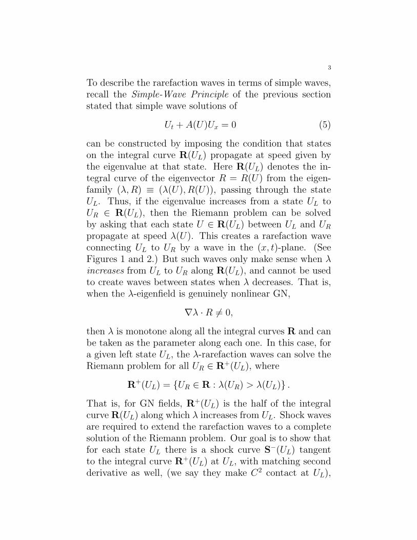
To describe the rarefaction waves in terms of simple waves,recall the Simple-Wave Principle of the previous sectionstated that simple wave solutions of

Ut + A(U)Ux = 0 (5)

can be constructed by imposing the condition that stateson the integral curve R(UL) propagate at speed given bythe eigenvalue at that state. Here R(UL) denotes the in-tegral curve of the eigenvector R = R(U) from the eigen-family (λ,R) ≡ (λ(U), R(U)), passing through the stateUL. Thus, if the eigenvalue increases from a state UL toUR ∈ R(UL), then the Riemann problem can be solvedby asking that each state U ∈ R(UL) between UL and URpropagate at speed λ(U). This creates a rarefaction waveconnecting UL to UR by a wave in the (x, t)-plane. (SeeFigures 1 and 2.) But such waves only make sense when λincreases from UL to UR along R(UL), and cannot be usedto create waves between states when λ decreases. That is,when the λ-eigenfield is genuinely nonlinear GN,

∇λ ·R 6= 0,

then λ is monotone along all the integral curves R and canbe taken as the parameter along each one. In this case, fora given left state UL, the λ-rarefaction waves can solve theRiemann problem for all UR ∈ R+(UL), where

R+(UL) = {UR ∈ R : λ(UR) > λ(UL)} .That is, for GN fields, R+(UL) is the half of the integralcurve R(UL) along which λ increases from UL. Shock wavesare required to extend the rarefaction waves to a completesolution of the Riemann problem. Our goal is to show thatfor each state UL there is a shock curve S−(UL) tangentto the integral curve R+(UL) at UL, with matching secondderivative as well, (we say they make C2 contact at UL),

4

such that the concatenation

W (UL) = R+(UL) ∪ S−(UL)

creates a wave curve along which the Riemann problem canbe solved whether λ increases or decreases from UL to URalongW (UL). (See Figures 1 and 3.) We will show that eachof the characteristic families of the p-system completes tosuch a wave curve Wi(UL), i = 1, 2, and the concatenationof these wave curves provides a coordinate system in U -space centered at UL that tells how to solve the Riemannproblem for every UR. The solution is unique within the theclass of admissible shock waves and rarefaction waves.

An important point to make is that the theory of shockwaves only applies to equations in conservation form,

Ut + f(U)x = 0, (6)

in which a total derivative falls on the nonlinear function f ,c.f. (10)). But the simple-wave form of the equations (5),not the conservation form (6), is required to describe thesimple-waves. To get the simple wave form of the equationsfrom the conservation form we must differentiate the fluxf with respect to U and then U with respect to x, That is,

∂f

∂x=∂f

∂U

∂U

∂x= A(U)Ux.

For a system of conservation laws in which U = (U1, ..., Un)and f(U) = (f1(U), ..., fn(U)), the matrix A(U) is denoteddf , and is simply the matrix obtained by putting the gra-dient ∇fi(U) in the i′th row to create an n × n matrix ofderivatives of f . Below we will use the conservation formof the equations to determine the shock waves, and thesimple-wave form of the equations to determine the rar-efaction waves, for Burgers equation and the p-system.

5

UL

UR

R+(UL)

U1

U2

U(λ)

λ

Figure 1: States on a λ-simple wave

x

t

UL

UL

UR

UR

dx

dt=

λ(U)

Figure 2: Centered Simple-Wave=Rarefaction Wave

6

Figure 3: The Wave Curve W(UL)

UL

UR

R+(UL)

U1

U2

λ

R−(UL) S−(UL)W(UL) = R+(UL) ∪ S−(UL)

2. The Rankine-Hugoniot Jump Condition forShock Waves

The principle for describing shock waves is the Rankine-Hugoniot (RH) jump condition. The RH condition appliesto solutions U(x, t) of equations in conservation form

Ut + f(U)x = 0, (7)

when U(x, t) is smooth on either side of a smooth curve(x(t), t) in the (x, t)-plane, but jumps from UL(t) to UR(t)across it. (See Figure 4.) In particular, when UL and URare constant, RH implies the speed s is constant as well.We will derive (7) as one of the applications of the diver-gence theorem in the next section, but for now we acceptit. The Rankine-Hugoniot jump condition states that tobe a legitimate shock wave, the speed of the shock s = xmust, at every time t, be related to the jump in u across

7

the shock by the relation

s[U ] = [f(U)]. (8)

The standard notation here is that brackets around a quan-tity [·] indicate the jump in the quantity from left to rightacross the shock, (left and right measured in the (x, t)-plane), so that [U ] = UR−UL and [f(U)] = f(UR)−f(UL).(See Figure 4.)

For example, the conservation form of the Burgers equationis

ut +

(1

2u2)x

= 0,

with flux function

f(u) =1

2u2.

In this case the role of RH is to give the speed of a shock interms of the right and left states. That is, solving for thespeed s in RH for Burgers equation gives an expression forthe shock speed in terms of the right and left states acrossa Burgers shock:

s =[f ]

[u]=

1

2

u2R − u2

L

uL − uR =uL + uR

2.

Conclude that for the scalar Burgers equation, the RH con-ditions simply tell us that the speed of a legitimate shockmust be the average of the states on the left and right ofthe shock. For system of equations, unraveling the meaningof the RH condition (8) is more problematic. A number ofcomments are in order.

8

t

x

UR ≡ UR(t)UL ≡ UL(t)

s ≡ x(t)

s[U ] = [f(U)]

Figure 4: The Rankine-Hugoniot Jump Condition for Shocks

• Note that the fundamental starting point of the theory ofshock waves is the conservation form of the equations (7).The RH jump condition (8) only makes sense for equationsin conservation form. It tells the quantities that are con-served, and these determine conservation across the shockwaves. As an example, multiplying Burgers through by ugives

(u2)t +

(2

3u3)x

= 0,

which has the same simple-wave form

ut + uux = 0,

but the conserved quantity is u2 not u, so the RH conditionis not the same condition. Thus, the conservation form ofthe equations is determined by the physically meaningful

9

quantities that are conserved. For example, the conserva-tion form of the compressible Euler equations is

ρt +Gx = 0,

Gt + (G2/ρ+ p)x = 0, (9)

of form

Ut + f(U)x = 0,

(upper case U to distinguish from the velocity u!), withU = (ρ,G) and f(U) = (G,G2/ρ + p). Since mass andmomentum are what is conserved across a shock wave, andthe conserved quantities are the mass density ρ and mo-mentum density G = ρu, these are the physically correctconserved quantities and hence this is the physically correctconservation form of the equations.

• Finally, note that if states UL = U1 and UR = U2 meetthe RH conditions

s[U ] = [f(U)],

then minus-ing the jumps on both sides shows UL = U2and UR = U1 does also...the RH conditions can’t distinguishbetween UL on the left and UR on the right, and the reverse.But in fact, only one of these will produce a stable shockwave. A large part of the theory of shock waves involvesthe study of entropy conditions that rule out the unstableshocks that have UL and UR on the wrong side. We willpresently see how to do this for the Burgers equation andfor the p-system and compressible Euler equations of gasdynamics.

3. The Riemann Problem for Burgers Equation

The Riemann problem is the initial value problem whenthe initial data consists of two constant states uL and uRseparated by a jump discontinuity at x = 0. (We use lower

10

case u for the unknown because it is a scalar.) That is, theinitial value problem

ut + f(u)x = 0, (10)

u(x, 0) = u0(x), (11)

where

u0(x) =

{uL, for x ≤ 0,uR, for x ≥ 0.

First, we can construct the rarefaction wave solutions ofthe Riemann problem when uL < uR from the Simple-WavePrinciple. To obtain the simple wave form of the equationsfrom the conservation form, differentiate the flux. That is,for a general scalar conservation law

ut + f(u)x = 0,

differentiate f by the chain rule to obtain

f(u)x = f ′(u)ux.

Thus the simple wave principle says λ = f ′(u), R = 1,and simple waves are constructed by asking that solutionsu(x, t) be constant along lines of speed x = λ. In the caseof Burgers equation,

f(u) =1

2u2,

and so the simple-wave form of Burgers equation is

ut + uux = 0.

Thus Burgers equation expresses that u(x, t) should be con-stant along lines of speed x = u, and so for Burgers we canconstruct the rarefaction wave solutions of the Riemannproblem when uL < uR by asking that each value of ubetween uL and uR should propagate at speed u: Such asolution creates a wave fan, or rarefaction wave, taking uLto uR. When uL > uR, the rarefaction waves don’t exist

11

because the speeds decrease from left to right, and the fanof values expands inconsistently back toward uL. In thiscase we take the shock wave solution that takes uL to uR.As above, according to the RH condition, the speed of theshock is the average of the speeds on each side,

s =[f ]

[u]=uL + uR

2.

Taking rarefaction waves when uL < uR and shock waveswhen uL > uR solves the Riemann problem for every uL, uR.The solution is pictured most easily in on the graph of fas a function of u, (see Figure 5). By the simple-waveformulation,

ut + f ′(u)ux = 0,

the speed of a wave is λ = f ′(u), which for Burgers happensto be f ′(u) = u. Thus the rarefaction wave speeds for statesu between uL and uR > uL are the slopes of the tangentlines of f at u, these slopes increasing as u increases fromuL to uR. The shock waves, on the other hand, have a speedgiven by the slope of the chord between uL and uR < ULbecause

s =[f ]

[u].

This picture for getting the speeds of states that solve theRiemann problem from the graph of f applies to any scalarconservation law of form

ut + f(u)x = 0,

subject to f ′′(u) > 0, the condition for GN. It only remainsto discuss the admissibility condition, or entropy conditionthat rules out the shock waves when uL < uR, allowable bythe RH condition alone.

12

Figure 5: Riemann Problem for Scalar Conservation Law ut + f(u)x = 0

uuL uR

f(u)

u

λ = f �(u)

s =f(uL)− f(uR)

uL − uR

• The main condition that picks out the shocks uL > uRfor Burgers equation is the so called Lax entropy condition.This states that characteristics should impinge on the shockfrom both sides, c.f. Figure 6. Mathematically, this statesthat an admissible shock should satisfy

λR < s < λL. (12)

Essentially, this rules out shocks in which the wave speedcan increase from uL to uR, because a rarefaction wavecould replace the shock wave as a solution of the Riemannproblem in this case. The shock wave is not allowed whena smoother solution exists. A shock that can be replacedby a rarefaction wave is called a rarefaction shock. Suchshocks are unstable because, under small perturbation ofthe initial data, the solution would find the simple wavefrom uL to uR, not the shock wave—and the rarefactionwave is not a small perturbation of the shock wave.

13

In contrast to rarefaction shock, Lax shocks are highly sta-ble. Since characteristics impinge on the shock, a smallpurturbation would send the solution constant along char-acteristics, right back into the shock. Moreover, we showedthat when you linearize the constant state in Burgers equa-tion, the purturbations evolve with almost the same wavespeed. Thus all small perturbations of uL and uR will getswept into the shock wave as the characteristics impingeon the shock. In particular, admissible Lax shocks destroyinformation as they propagate...information about the pastis lost as characteristics impinge on the shock. See Figure 6for how all information about the initial data except uL anduR can be lost by characteristics impinging on the shock.It follows that when shock waves are present, the past can-not be recovered from the present, and the solutions are nolonger time-reversible. One can show that this loss of in-formation in the compressible Euler equations correspondsto increase of entropy, a thermodynamical measure of in-formation lost.

14

t

x

Shock Wave

LeftCharacteristics

RightCharacteristics

Lost Information

Figure 6: Characteristics Impinge on a Lax ShockWith Consequent Loss of Information

4. The Riemann Problem for the p-system

We now solve the Riemann problem for the p-system underthe assumptions that

p′(v) < 0, p′′(v) > 0. (13)

The first condition just states that pressure rises with den-sity ρ = 1/v, and the second guarantees genuine nonlinear-ity in both characteristic fields, c.f. Section 8. In particular,the isothermal equations of state

p =σ2

v

meets both conditions (13).

To start, recall that the p-system is the nonlinear waveequation with sound speed c(v) =

√−p′(v), and is ob-tained from the compressible Euler equations by changing

15

the spatial coordinate to a frame moving with the fluid ateach point. The p-system takes the conservation form(

vu

)t

+

( −up(v)

)x

= 0., (14)

of form (10) with conserved quantities U = (v, u) and fluxf(U) = (−u, p(v)). The p-system is physically equivalent tothe compressible Euler equations, and in particular it canbe shown that the RH jump conditions determine the sameshock curves with transformed shock speeds. Because it issimpler, we now derive the shock curves for the p-system,and see how they connect with the rarefaction curves R+

derived in the previous section.

To construct the shock curves S(UL), we solve for the set ofright states U = (v, u) that meet the RH jump conditionss[U ] = [f(U)] with left state UR = (vL, uR), and some speeds. This defines the so called Hugoniot locus of UL, the setof all possible states that can be connected to UL across ashock wave. Putting (14) into RH gives

s[U ]− [f(U)] = s

(v − vLu− uL

)−(

uL − up(v)− p(vL)

)= 0,

yielding the two equations

s(v − vL) = −(u− uL), (15)

s(u− uL) = p(v)− p(vL).

Multiplying both sides of (15) and (16) together gives

s2 = −p(v)− p(vL)

v − vL = −p′(v∗), (16)

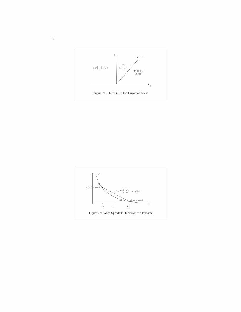
where the mean value theorem gives the existence of v∗ =v∗(vL, v) between vL and v. (See Figure 7b.)

16

x

t

UL

Figure 7a: States U in the Hugoniot Locus

(vL, uL)

(v, u)U ≡ UR

x = s

s[U ] = [f(U)]

v

p(v)

vL vR

−s2 =p(v)− p(vL)

v − vL

−c(vL)2 = p�(vL)

−c(vR)2 = p�(vR)

v∗

= −p�(v∗)

Figure 7b: Wave Speeds in Terms of the Pressure

17

Thus the shock speeds are

s = ±√−p(v)− p(vL)

v − vL = ±√−p′(v∗), (17)

Since

limv→vL

√−p′(v∗) = ±

√−p′(vL) = ±c(vL), (18)

we set the 1-shock speed equal to

s1 ≡ s1(vL, v) = −√−p′(v∗), (19)

and the 2-shock speed equal to

s2 ≡ s2(vL, v) = −√−p′(v∗). (20)

To obtain the shock curves, eliminate s from (15), (16) toobtain

(u− uL)2 = −(p(v)− p(vL))(v − vL), (21)

or

u = uL ±√−(p(v)− p(vL))(v − vL)

= uL ±√−p(v)− p(vL)

v − vL (v − vL)

= uL ±√−p′(v∗)(v − vL).

Note that because p′(v) < 0, all functions under squareroot signs are positive.

Now define the 1-shock curve S1 by,

u = uL +√−(p(v)− p(vL))(v − vL)

or

S1 : u = uL +√−p′(v∗).

and the 2-shock curve S2 as

u = uL −√−(p(v)− p(vL))(v − vL),

18

or

S2 : u = uL +√−p′(v∗).

Now it is clear that S1 gives the curve of states U that makeshocks with UL of negative speed s1, and S2 gives the curveof states U that make shocks with UL of positive speed s2.To see this, note that by (15),

s = −u− uLv − vL ,

so when s = s1 < 0 we have

−u− uLv − vL < 0,

meaning we must be on S1, and when s = s2, we have

−u− uLv − vL > 0,

meaning we must be on S1.

Now recall

R1(UL) = R1(UL)− ∪R+1 (UL),

R2(UL) = R−2 (UL) ∪R+2 (UL),

where R+1 (UL) and R+

2 (UL) are the 1- and 2- rarefactioncurves passing through the state UL, that portion of theintegral curves along which the eigenvalues increase, so theportion that corresponds to viable right states for rarefac-tion waves starting with left state UL.

Similarly, define

S1(UL) = S1(UL)− ∪ S+1 (UL),

S2(UL) = S−2 (UL) ∪ S+2 (UL),

as diagrammed in Figure 8. We now prove the followingtheorem:

19

Theorem 1. For each UL, the 1-shock curve S1(UL) inter-sects R1(UL) at the state UL, at which point the two curveshave equal first and second derivative. Similarly, the 2-shock curve S2(UL) intersects R2(UL) at the state UL, andthese latter two curves are also have equatl first and secondderivatives at UL. We say that the shock curves have C2

tangency with the rarefaction curves at UL.

The tangency of the shock and rarefaction curves is dia-grammed in Figure 9. The theorem completes the pictureof the shock and rarefaction curves. I.e., the shock curveS−1 (UL) completes the rarefaction curve R+

1 (UL) to a C2

1-wave curve W1(UL) defined by, (c.f. Figure 10),

W1(UL) = S−1 (UL) ∪R+1 (UL).

Similarly, define 2-wave curve W1(UL), also C2, is definedby

W1(UL) = S−1 (UL) ∪R+1 (UL).

Moreover, it follows from Figure 7b that the i-characteristicsimpinge on the i-shock waves like Figure 6, thereby meet-ing the Lax admissibility for shock waves, precisely whenUR is on S−i . Finally, it is easy to see that the wave curvesstay within the physical domain v > 0.

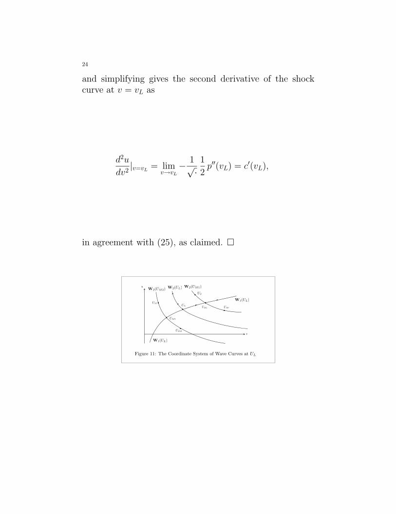
Before giving the proof of Theorem 1, we can complete theresolution of the Riemann problem by defining a coordi-nate system of wave curves based at UL. For this, draw all2-wave curves W2(UM) for UM ∈W1(UL), as diagrammedin Figure 11. Then for any right state U = UR, we cansolve the Riemann problem by finding the state UM suchthat UL ∈W2(UM). Then the Rieman problem is resolvedby the negative speed 1-wave from UL to UM , followed bya positive speed 2-wave from UM to UL. The waves are ei-ther shock waves or rarefaction waves depending on whichregion (I-IV) UR lies in relative to the coordinate systemof wave curves at UL, (see Figure 11). The various cases

20

are diagrammed in Figures 12-15. Examples of wave inter-actions that can be resolved by Riemann problems aloneare diagrammed in Figures 16,17. It is not so difficult tojustify that for isothermal gas dynamics p = σ2/v, this pro-cedure produces a unique solution of the Riemann problemin the class of shock waves and rarefaction waves. A com-plete proof of uniqueness of solutions would entail showingthat two wave curves W2(UM1) never intersects W2(UM2 forUM1 6= UM2 on W1(UL). This is true for any p satisfyingp′(v) < 0, p′′(v) > 0. To prove existence of a solution forevery UR, entails proving that every state UR in the phys-ical domain v > 0, can be reached by W2(UM), for someUM on W1(UL). It is not so difficult to show that this istrue for the isothermal equation of state. But for moregeneral equations of state, (like polytropic gases satisfyingp = 1/vγ, γ > 1), this is not strictly true because of thepossible formation of vacuum states. See [Smoller] for amore in depth discussion of the very interesting issue of thevacuum.

21

u

v

UL

S−2 (UL)

S−1 (UL)

vL

S+1 (UL)

S+2 (UL)

u− uL +

�−p(v)− p(vL)

v − vL

(v − vL)

u− uL −�− p(v)− p(vL)v − vL (v − vL)

v < vL v > vL

Figure 8: The Shock Curves for the p-system.

u

v

UL

R+1 (UL)

R+2 (UL)

S−2 (UL)

S−1 (UL)

S+1 (UL)

S+2 (UL)

R−1 (UL)

R−2 (UL)

I

II

III

IV

Figure 9: The Shock and Rarefaction Curves for the p-system.

22

u

v

UL

R+1 (UL)

R+2 (UL)

S−2 (UL)

S−1 (UL)

I

II

III

IV

vL

Figure 10: The Wave Curves of the p-system

• Proof of Theorem 1: We show that the 1-rarefactioncurve is tangent to the 1-shock curve at U = UL, the caseof 2 shocks being similar. Recall then that the 1-integralcurves are given by

s = u− h(v) = const,

so

u = h(v) + const, (22)

where

h′(v) = c(v) =√−p′(v).

The 1-shock curve is given by

u = uL +

√−p(v)− p(vL)

v − vL (v − vL). (23)

23

We check agreement of the first two derivatives at v = vL.First, along (22),

du

dv= h′(v) = c(v),

d2u

dv2 = c′(v),

so at v = vL we have

du

dv= c(vL),

d2u

dv2 = c′(vL). (24)

On the other hand, for the shock curve (23) we compute

du

dv=

d

dv

√−p(v)− p(vL)

v − vL · (v − vL) +

√−p(v)− p(vL)

v − vLso at v = vL we have

du

dv= lim

v→vL

√−p(v)− p(vL)

v − vL =√−p′(vL) = c(vL), (25)

in agreement with (25). To verify agreement at the secondderivative, differentiate (26) by the product rule to obtain

d2u

dv2 =d2

dv2

√·(v − vL) + 2d

dv

√·.Since the first term will vanish when v = vL, we get

d2u

dv2 |v=vL= lim

v→vL

2d

dv

√−p(v)− p(vL)

v − vL .

But

2d

dv

√−p(v)− p(vL)

v − vL =−1√·

(v − vL)p′(v)− (p(v)−p(vL)v−vL

v − vL .

Substituting the Taylor approximation

p(v) = p(vL) + p′(vL)(v − vL) +O(v − vL)2,

24

and simplifying gives the second derivative of the shockcurve at v = vL as

d2u

dv2 |v=vL= lim

v→vL

− 1√·1

2p′′(vL) = c′(vL),

in agreement with (25), as claimed. �

u

v

UL

W1(UL)

W2(UL) W2(UM1)W2(UM2)

UM2

UM1

UII

UI

UIII

UIV

W1(UL)

Figure 11: The Coordinate System of Wave Curves at UL

25

x

t

UL UR

Figure 12: The Riemann Solution for Region I

UM2

x

t

UL UR

Figure 13: The Riemann Solution for Region II

UM1

26

x

t

UL UR

Figure 14: The Riemann Solution for Region III

UM2

x

t

UL UR

Figure 15: The Riemann Solution for Region IV

UM2

27

x

t

UL UR

UL UR

UM

UM1

Figure 16: A 1-Shock Interacts With a 2-Shock

x

t

UL UR

UL UR

UM

UM1

Figure 17: Two 2-Shocks Reflect a 1-rarefactions wave