9 FREE VIBRATION AND EARTHQUAKE ANALYSIS OF A BUILDING · 2020. 2. 26. · FREE VIBRATION AND EARTHQUAKE ANALYSIS OF A BUILDING 15 m 15 m 25 m 3 m Figure 9.1 Geometry of the model

TUTORIAL MANUAL

9 FREE VIBRATION AND EARTHQUAKE ANALYSIS OF A BUILDING

This example demonstrates the natural frequency of a long five-storey building whensubjected to free vibration and earthquake loading. The two calculations employ differentdynamic boundary conditions:

• In the free vibration, the Viscous boundary conditions are considered. This option issuitable for problems where the dynamic source is inside the mesh.

• For the earthquake loading, the Free-field and Compliant base boundary conditionsare considered. This option is preferred for earthquake analysis, where the dynamicinput is applied along the model boundary.

The building consists of 5 floors and a basement. It is 10 m wide and 17 m high includingthe basement. The total height from the ground level is 5 x 3 m = 15 m and the basementis 2 m deep. A value of 5 kN/m2 is taken as the weight of the floors and the walls. Thebuilding is constructed on a clay layer of 15 m depth underlayed by a deep sand layer. Inthe model, 25 m of the sand layer will be considered.

Objectives:

• Performing a Dynamic calculation

• Defining dynamic boundary conditions (free-field and compliant base)

• Defining earthquakes by means of displacement multipliers

• Modelling of free vibration of structures

• Modelling of hysteretic behaviour by means of HS small model

• Calculating the natural frequency by means of Fourier spectrum

9.1 GEOMETRY

The length of the building is much larger than its width and the earthquake is supposed tohave a dominant effect across the width of the building. Taking these facts intoconsideration, a representative section of 3 m will be considered in the model in order todecrease the model size. The geometry of the model is shown in Figure 9.1.

9.1.1 GEOMETRY MODEL

• Start the Input program and select Start a new project from the Quick select dialogbox.

• In the Project tabsheet of the Project properties window, enter an appropriate title.

• Keep the default units and set the model dimensions to Xmin = −80, Xmax = 80, Ymin= 0 and Ymax = 3.

9.1.2 DEFINITION OF SOIL STRATIGRAPHY

The subsoil consists of two layers. The Upper clayey layer lies between the ground level(z = 0) and z = -15. The underlying Lower sandy layer lies to z = -40. Define the phreaticlevel by assigning a value of -15 to the Head in the borehole. Create the material data set

120 Tutorial Manual | PLAXIS 3D 2018

FREE VIBRATION AND EARTHQUAKE ANALYSIS OF A BUILDING

15 m

15 m

25 m

3 m

Figure 9.1 Geometry of the model

according to Table 9.1 and assign it to the corresponding soil layers. The upper layerconsists of mostly clayey soil and the lower one consists of sandy soil.

Table 9.1 Material properties of the subsoil layers

Parameter Name Upper clayey layer Lower sandy layer Unit

General

Material model Model HS small HS small -

Drainage type Type Drained Drained -

Soil unit weight above phreatic level γunsat 16 20 kN/m3

Soil unit weight above phreatic level γsat 20 20 kN/m3

Parameters

Secant stiffness in standard drained triaxial test E ref50 2.0·104 3.0·104 kN/m2

Tangent stiffness for primary oedometer loading E refoed 2.561·104 3.601·104 kN/m2

Unloading / reloading stiffness E refur 9.484·104 1.108·105 kN/m2

Power for stress-level dependency of stiffness m 0.5 0.5 -

Cohesion c'ref 10 5 kN/m2

Friction angle ϕ' 18.0 28.0 ◦

Dilatancy angle ψ 0.0 0.0 ◦

Shear strain at which Gs = 0.722G0 γ0.7 1.2·10-4 1.5·10-4 -

Shear modulus at very small strains Gref0 2.7·105 1.0·105 kN/m2

Poisson's ratio ν 'ur 0.2 0.2 -

When subjected to cyclic shear loading, the HS small model will show typical hystereticbehaviour. Starting from the small-strain shear stiffness, Gref

0 , the actual stiffness willdecrease with increasing shear. Figures 9.2 and 9.3 display the Modulus reductioncurves, i.e. the decay of the shear modulus with strain.

PLAXIS 3D 2018 | Tutorial Manual 121

TUTORIAL MANUAL

0

100000

50000

150000

200000

250000

She

arm

odul

us

Shear strain0.00001 0.0001 0.001 0.01

Gt Gsγ0.7

0.722G0

G used

Figure 9.2 Modulus reduction curves for the upper clayey layer

20000

40000

60000

80000

100000

She

arm

odul

us

Shear strain0.00001 0.0001 0.001 0.01

GtGs

γ0.7

0.722G0

G used

Figure 9.3 Modulus reduction curve for the lower sandy layer

In the HS small model, the tangent shear modulus is bounded by a lower limit, Gur .

Gur =Eur

2(1 + νur )

The values of Grefur for the Upper clayey layer and Lower sandy layer and the ratio to Gref

0are shown in Table 9.2. This ratio determines the maximum damping ratio that can beobtained.

Table 9.2 Gur values and ratio to Gref0

Parameter Unit Upper clayeylayer

Lower sandylayer

Gur kN/m2 39517 41167

Gref0 /Gur - 6.83 2.43

Figures 9.4 and 9.5 show the damping ratio as a function of the shear strain for thematerial used in the model. For a more detailed description and elaboration from the



modulus reduction curve to the damping curve can be found in the literature∗.

0

0.2

0.15

0.1

0.05Dam

ping

ratio

Cyclic shear strain0.00001 0.0001 0.001 0.01

Figure 9.4 Damping curve for the upper clayey layer

0

0.2

0.15

0.1

0.05

Dam

ping

ratio

Cyclic shear strain0.00001 0.0001 0.001 0.01

Figure 9.5 Damping curve for the lower sandy layer

9.1.3 DEFINITION OF STRUCTURAL ELEMENTS

The structural elements of the model are defined in the Structures mode.

Building

The building consists of 5 floors and a basement. It is 10 m wide and 17 m high includingthe basement. The total height from the ground level is 5 x 3 m = 15 m and the basementis 2 m deep. A value of 5 kN/m2 is taken as the weight of the floors and the walls. Todefine the structure:

Define a surface passing through the points (-5 0 -2), (5 0 -2), (5 3 -2) and (-5 3 -2).

Create a copy of the surface by defining an 1D array in z-direction. Set the numberof the columns to 2 and the distance between them to 2 m.

Select the created surface at z = 0 and define a 1D array in the z-direction. Set thenumber of the columns to 6 and the distance between consecutive columns to 3 m.

Define a surface passing through the points (5 0 -2), (5 3 -2), (5 3 15) and (5 0 15).

∗ Brinkgreve, R.B.J., Kappert, M.H., Bonnier, P.G. (2007). Hysteretic damping in small-strain stiffness model. InProc. 10th Int. Conf. on Comp. Methods and Advances in Geomechanics. Rhodes, Greece, 737− 742


TUTORIAL MANUAL

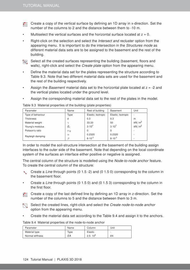
Create a copy of the vertical surface by defining an 1D array in x-direction. Set thenumber of the columns to 2 and the distance between them to -10 m.

• Multiselect the vertical surfaces and the horizontal surface located at z = 0.

• Right-click on the selection and select the Intersect and recluster option from theappearing menu. It is important to do the intersection in the Structures mode asdifferent material data sets are to be assigned to the basement and the rest of thebuilding.

Select all the created surfaces representing the building (basement, floors andwalls), right-click and select the Create plate option from the appearing menu.

• Define the material data set for the plates representing the structure according toTable 9.3. Note that two different material data sets are used for the basement andthe rest of the building respectively.

• Assign the Basement material data set to the horizontal plate located at z = -2 andthe vertical plates located under the ground level.

• Assign the corresponding material data set to the rest of the plates in the model.

Table 9.3 Material properties of the building (plate properties)

Parameter Name Rest of building Basement Unit

Type of behaviour Type Elastic; Isotropic Elastic; Isotropic -

Thickness d 0.3 0.3 m

Material weight γ 33.33 50 kN/m3

Young’s modulus E1 3·107 3·107 kN/m2

Poisson’s ratio ν12 0 0 -

Rayleigh dampingα 0.2320 0.2320 -

β 8·10-3 8·10-3 -

In order to model the soil-structure intersection at the basement of the building assigninterfaces to the outer side of the basement. Note that depending on the local coordinatesystem of the surfaces an interface either positive or negative is assigned.

The central column of the structure is modelled using the Node-to-node anchor feature.To create the central column of the structure:

Create a Line through points (0 1.5 -2) and (0 1.5 0) corresponding to the column inthe basement floor.

• Create a Line through points (0 1.5 0) and (0 1.5 3) corresponding to the column inthe first floor.

Create a copy of the last defined line by defining an 1D array in z-direction. Set thenumber of the columns to 5 and the distance between them to 3 m.

Select the created lines, right-click and select the Create node-to-node anchoroption from the appearing menu.

• Create the material data set according to the Table 9.4 and assign it to the anchors.

Table 9.4 Material properties of the node-to-node anchor

Parameter Name Column Unit

Material type Type Elastic -

Normal stiffness EA 2.5· 106 kN



Loads

A static lateral force of 10 kN/m is applied laterally at the top left corner of the building. Tocreate the load:

Create a line load passing through (-5 0 15) and (-5 3 15).

• Specify the components of the load as (10 0 0).

The earthquake is modelled by imposing a prescribed displacement at the bottomboundary. To define the prescribed displacement:

Create a surface prescribed displacement passing through (-80 0 -40), (80 0 -40),(80 3 -40) and (-80 3 -40).

• Specify the x-component of the prescribed displacement as Prescribed and assigna value of 1.0. The y and z components of the prescribed displacement are Fixed.The default distribution (Uniform) is valid.

To define the dynamic multipliers for the prescribed displacement:

• In the Model explorer expand the Attributes library subtree. Right-click on Dynamicmultipliers and select the Edit option from the appearing menu. The Multiplierswindow pops up displaying the Displacement multipliers tabsheet.

To add a multiplier click the corresponding button in the Multipliers window.

• From the Signal drop-down menu select the Table option.

• The file containing the earthquake data is available in the PLAXIS knowledge base(http://kb.plaxis.nl/search/site/smc).

• Open the page in a web browser, copy all the data to a text editor (e.g. Notepad)and save the file in your computer with the extension ∗.smc. Alternatively this filecan also be found in the Importables folder in the PLAXIS directory.

In the Multipliers window click the Open button and select the saved file. In theImport data window select the Strong motion CD-ROM files option from the Parsingmethod drop-down menu and press OK to close the window.

• Select the Acceleration option in the Data type drop-down menu.

• Select the Drift correction options and click OK to finalize the definition of themultiplier.

• In the Dynamic multipliers window the table and the plot of the data is displayed(Figure 9.6).

• In the Model explorer expand the Surface displacements subtree and assign theMultiplierx to the x- component by selecting the option in the drop-down menu.

Create interfaces on the boundary

Free-field and Compliant base require the manual creation of interface elements alongthe vertical and bottom boundaries of the model in the Structures mode. The interfaceelements must be added inside the model, else the Free-field and Compliant baseboundary conditions are ignored. To define the interfaces:

Create a surface passing through (-80 3 0), (-80 0 0), (-80 0 -40) and (-80 3 -40).Right-click the created surface and and click Create positive interface to add an


TUTORIAL MANUAL

Figure 9.6 Dynamic multipliers window

interface inside the model.

Create a surface passing through (80 3 0), (80 0 0), (80 0 -40) and (80 3 -40).Right-click the created surface and and click Create negative interface to add aninterface inside the model.

• The surface at the bottom of the model is already created by the prescribeddisplacement. Right-click the surface at the bottom of the model and click Createpositive interface to add an interface inside the model.

9.2 MESH GENERATION

• Proceed to the Mesh mode.

• Click the Generate mesh button. Set the element distribution to Fine.

• View the generated mesh (Figure 9.7).



Figure 9.7 Geometry and mesh

9.3 PERFORMING CALCULATIONS

The calculation process consists of the initial conditions phase, simulation of theconstruction of the building, loading, free vibration analysis and earthquake analysis.

Initial phase

• Click on the Staged construction tab to proceed with definition of the calculationphases.

• The initial phase has already been introduced. The default settings of the initialphase will be used in this tutorial.

• In the Staged construction mode check that the building and load are inactive.

Phase 1

Add a new phase (Phase_1). The default settings of the added phase will be usedfor this calculation phase.

• In the Staged construction mode construct the building (activate all the plates, theanchors and only the interfaces of the basement) and deactivate the basementvolume (Figure 9.8).

Phase 2

Add a new phase (Phase_2).

• In the Phases window select the Reset displacement to zero in the Deformationcontrol parameters subtree. The default values of the remaining parameters will beused in this calculation phase.

• In the Staged construction mode activate the line load. The value of the load isalready defined in the Structures mode.


TUTORIAL MANUAL

Figure 9.8 Construction of the building

Phase 3


In the Phases window select the Dynamic option as Calculation type.

• Set the Time interval parameter to 5 sec.

• In the Staged construction mode deactivate the line load.

• In the Model explorer expand the Model conditions subtree.

• Expand the Dynamics subtree. By default the boundary conditions in the x and ydirections are set to viscous. Select the None option for the boundaries in the ydirection. Set the boundary Zmin to viscous (Figure 9.9).

Figure 9.9 Boundary conditions for Dynamic calculations (Phase_3)



Hint: For a better visualisation of the results, animations of the free vibration andearthquake can be created. If animations are to be created, it is advised toincrease the number of the saved steps by assigning a proper value to theMax steps saved parameter in the Parameters tabsheet of the Phaseswindow.

Phase 4


• In the Phases window set the Start from phase option to Phase 1 (construction ofbuilding).

Select the Dynamic option as Calculation type.

• Set the Dynamic time interval parameter to 20 sec.

• Select the Reset displacement to zero in the Deformation control parameterssubtree. The default values of the remaining parameters will be used in thiscalculation phase.

• In the Numerical control parameters subtree uncheck the Use default iterparameters checkbox, which allows you to change advanced settings and set theTime step determination to Manual.

• Set the Max steps to 1000 and the Max number of sub steps to 4.

• In the Model explorer expand the Model conditions subtree.

• Expand the Dynamics subtree. Set the Free-field option for the boundaries in the xdirection. The boundaries in the y direction are already set to None. Set theboundary Zmin to Compliant base (Figure 9.10).

• Make sure that the interfaces on the boundary of the model are not activated in theModel explorer.

• In the Model explorer activate the Surface displacement and its dynamiccomponent. Set the value of ux to 0.5 m. Considering that the boundary condition atthe base of the model will be defined using a Compliant base, the input signal has tobe taken as half of the outcropping motion.

Select points for load displacement curves at (0 1.5 15), (0 1.5 6), (0 1.5 3) and (01.5 -2). The calculation may now be started.


TUTORIAL MANUAL

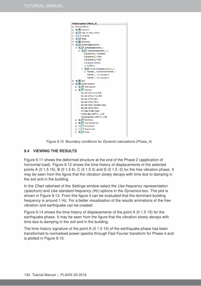
Figure 9.10 Boundary conditions for Dynamic calculations (Phase_4)

9.4 VIEWING THE RESULTS

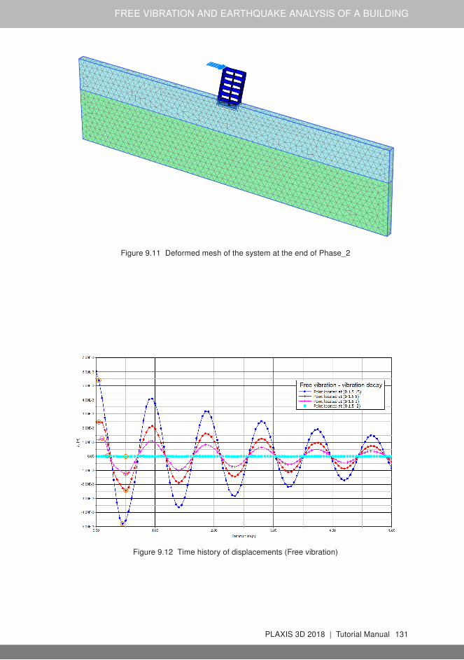
Figure 9.11 shows the deformed structure at the end of the Phase 2 (application ofhorizontal load). Figure 9.12 shows the time history of displacements of the selectedpoints A (0 1.5 15), B (0 1.5 6), C (0 1.5 3) and D (0 1.5 -2) for the free vibration phase. Itmay be seen from the figure that the vibration slowly decays with time due to damping inthe soil and in the building.

In the Chart tabsheet of the Settings window select the Use frequency representation(spectrum) and Use standard frequency (Hz) options in the Dynamics box. The plot isshown in Figure 9.13. From this figure it can be evaluated that the dominant buildingfrequency is around 1 Hz. For a better visualisation of the results animations of the freevibration and earthquake can be created.

Figure 9.14 shows the time history of displacements of the point A (0 1.5 15) for theearthquake phase. It may be seen from the figure that the vibration slowly decays withtime due to damping in the soil and in the building.

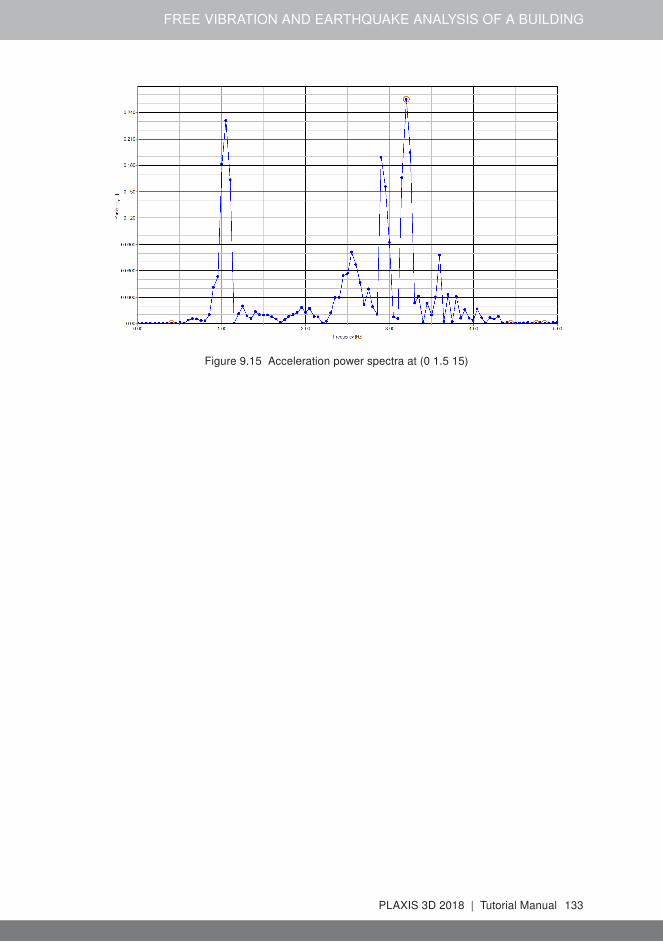
The time history signature of the point A (0 1.5 15) of the earthquake phase has beentransformed to normalised power spectra through Fast Fourier transform for Phase 4 andis plotted in Figure 9.15.



Figure 9.11 Deformed mesh of the system at the end of Phase_2

Figure 9.12 Time history of displacements (Free vibration)


TUTORIAL MANUAL

Figure 9.13 Frequency representation (spectrum - Free vibration)

Figure 9.14 Time history of displacements of the top of the building (Earthquake)



Figure 9.15 Acceleration power spectra at (0 1.5 15)


Documents

9 FREE VIBRATION AND EARTHQUAKE ANALYSIS OF A BUILDING · 2020. 2. 26. · FREE VIBRATION AND EARTHQUAKE ANALYSIS OF A BUILDING 15 m 15 m 25 m 3 m Figure 9.1 Geometry of the model