Embed Size (px)
Citation preview

1
2
3
4
5
6
7
8
9
10
11
12
13
14
15
16
17
18
19
20
A curious local surface salinity maximum in the
northwestern tropical Atlantic
Semyon A. Grodsky1, James A. Carton1, and Frank O. Bryan2
December 12, 2013
1Department of Atmospheric and Oceanic Science, University of Maryland, College Park
2National Center for Atmospheric Research, Boulder, CO
Corresponding author: [email protected] 21

Abstract 22
23
24
25
26
27
28
29
30
31
32
33
34
35
36
37
38
Sea surface salinity (SSS) measurements from the Aquarius/SACD satellite reveal
the seasonal development of a local salinity maximum in the northwestern tropical
Atlantic in boreal winter to early spring. This seasonal tropical SSS maximum, which is
confirmed by comparison to in situ observations, is centered at 8°N, and is up to 0.5 psu
saltier than the surrounding water despite its location in the latitude band of the highly
precipitating Intertropical Convergence Zone. Its existence seems to be the result of the
differing phases in the seasonal variations of Amazon discharge and ocean currents. In
late boreal fall - winter, when the discharge is at its minimum, but the North Brazil
Current (NBC) and its retroflection are still present, a mixture of high salinity water of
equatorial and South Atlantic origin is transported along the shelf break by the NBC
retroflecting into the western part of the North Equatorial Countercurrent (NECC). This
salt transport produces the salty signature of the western part of the NECC, which is seen
as a localized salinity maximum on satellite imagery, in contrast to the fresh signature
present in summer – early fall. The seasonal slowing/reversal of the NECC in boreal
spring stops this eastward salt transport, thus leading to the disappearance of this
northwestern tropical SSS maximum.
1

1. Introduction 39
40
41
42
43
44
45
46
47
48
49
50
51
52
53
54
55
56
57
58
59
60
61
A striking feature of the Atlantic Ocean is the appearance of pools of high salinity
( > 37psu) surface water in the subtropics of both hemispheres due to high rates of
evaporation and negligible rainfall, which are separated by lower salinity surface water in
the rainy tropics (e.g. Schmitt, 2008). The introduction of satellite remote sensing has
greatly expanded our ability to monitor the geographical and temporal variability of these
sea surface salinity (SSS) features and to detect their variations (Lagerloef et al., 2012).
Here we use these new remotely sensed observations to describe the seasonal appearance
of a poorly known secondary surface salinity maximum ( > 36.1psu) that lies within the
high precipitation tropical zone in the northwestern tropical Atlantic.
The seasonal storage of salt within the mixed layer in this region of the Atlantic is
controlled by several competing processes, all of which vary seasonally (Foltz et al.,
2004). Among these two major sources of freshwater have to be taken into account: high
precipitation under the Intertropical Convergence Zone (ITCZ), and the discharge of
major rivers along the northwestern coast of South America (e.g. Mignot et al., 2007).
Between the equator and 12°-15ºN mixed layer salinity, and thus SSS, is diluted by
freshwater input from the seasonally migrating atmospheric ITCZ, which reaches its
northernmost position in late boreal summer/fall (e.g. Xie and Carton, 2004). This fresh
mixed layer is advected both zonally (by the developing seasonal currents) and
meridionally (through Ekman transport by the seasonal trade winds). West of 40ºW
mixed layer salinity is significantly freshened by the spread of near-surface water from
the Amazon, whose discharge peaks in mid-May and decreases to its seasonal minimum
in mid-November, reflecting the seasonal march of the ITCZ and water storage processes
2

62
63
64
65
66
67
68
69
70
71
72
73
74
75
76
77
78
79
80
81
82
83
84
over the catchment area (Dai and Trenberth, 2002). By early boreal fall the spread of the
Amazon waters forms a 106 km2 fresh pool west of 40ºW (Dessier and Donguy, 1994),
producing near-surface barrier layers capable of affecting local air-sea interactions even
under hurricane-force winds (e.g. Grodsky et al., 2012). Barrier layers of up to 20 m
thickness have been found equatorward of roughly 10°N except in boreal winter (Mignot
et al., 2007).
In addition to surface freshwater flux, horizontal advection by seasonal currents
also plays an important role in the mixed layer salt balance (e.g. Foltz et al., 2004, Foltz
and McPhaden, 2008; Grodsky et al., 2014). Key features of the seasonal currents (e.g.
Richardson and Reverdin, 1987) include the westward flowing near-equatorial northern
branch of the South Equatorial Current whose transport peaks in boreal summer, and
feeds into the coastal North Brazil Current (NBC). The NBC transports this water, diluted
by discharge from the Amazon River, northwestward along the eastern boundary of
South America in boreal winter and spring. In summer, however, the shifting trade winds
allows the NBC to retroflect and be carried eastward in the developing North Equatorial
Countercurrent (NECC) at latitudes between 5°-10°N (e.g. Carton and Katz, 1990).
Indeed, from August through October typically 70% of the Amazon plume water is
deflected eastward in the NECC along the NBC retroflection (Lentz, 1995), thus
producing the fresh signature of the western part of the NECC present in summer – early
fall. The seasonal appearance of the fresh NECC and accompanying ITCZ rainfall
dramatically reduce mixed layer salinities in this band of latitudes (Muller-Karger et al.,
1988), causing a fresh barrier layer to develop within the mixed layer (e.g. Liu et al.,
2009). The western part of the NECC reaches its maximum eastward flow by boreal fall,
3

85
86
87
88
89
90
91
92
93
94
95
96
97
98
99
100
101
102
103
104
105
106
107
then slows so that in late boreal winter the direction of the surface current is westward.
As we shall see later, the seasonal changes of salinity of water carried by the NBC into
the NECC ultimately leads to the seasonal appearance of a local surface salinity
maximum pool in the western basin.
Until recently most of the information about these changes in salinity came from a
series of in situ observing programs such as the volunteer observing ship thermo-
salinograph (TSG) program (e.g. Dessier and Donguy, 1994), historical hydrography
available in the World Ocean Atlas series such as WOA09 (Boyer et al., 2012), as well as
the recently deployed Argo profiling floats (Roemmich et al., 2009). In the past several
years, this suite of in-situ salinity measurements has been complemented by observations
from two remote sensing instruments: the Soil Moisture and Ocean Salinity satellite in
late-2009 and Aquarius/SAC-D in spring 2011. Both instruments observe upwelling
radiation in the microwave L-band (1.4 GHz) and deduce salinity from the emissivity-
dependence on surface conductivity. In this study we examine Aquarius/SAC-D
observations, which have a spatial resolution of approximately 100 km (Lagerloef et al.,
2012). The results are diagnosed by comparison to salinity from more traditional
observing systems and an eddy resolving ocean numerical simulation.
2. Data and Methods
The main SSS data set used in this study is the daily level 3 version 2.3 Aquarius
SSS beginning 25 August, 2011, obtained from the NASA Jet Propulsion Laboratory
Physical Oceanography Distributed Active Archive Center on a 1°x1° grid (Lagerloef et
al., 2012), which spans only two full years so far. To emphasize features present during
both years, the Aquarius SSS climatology is evaluated using the Fourier series truncated
4

108
109
110
111
112
113
114
115
116
117
118
119
120
121
122
123
124
125
126
127
128
129
130
after the annual and semiannual harmonics. In the tropics where the seasonal variations
dominate, it is reasonable to examine such a SSS climatology based on only two years of
observations because of the dominance of the annual cycle (e.g. Xie and Carton, 2004).
We will illustrate the similarity of SSS between 2012 and 2013 later.
The Aquarius SSS data are used along with the salinity observations from four
buoys located between 4°N and 15°N along the 38°W meridian (Foltz et al., 2004).
These buoys, which are part of the Prediction and Research Moored Array in the Atlantic
(PIRATA) array (Bourlès et al., 2008), have been maintained continuously since 1997.
Salinity is typically available at four depths between 1 – 120m. We also use the monthly
WOA09 SSS climatology based on historical hydrographic observations (Boyer et al.,
2012); ship of opportunity TSG data collected along major merchant ship lanes (Dessier
and Donguy, 1994); and the uppermost measurement from Argo profiling floats
(typically at 5m to 10m depth) (Roemmich et al., 2009).
In the latitude band of the highly precipitating ITCZ much of the temporal
variability of net surface freshwater flux is due to the temporal variability of precipitation
(Yoo and Carton, 1990). We track variations in precipitation using a combination of the
Microwave Imager, and the Precipitation Radar, that form part of the Tropical Rainfall
Measuring Mission (TRMM) satellite sensor suite (trmm.gsfc.nasa.gov). We track
monthly continental discharge from the tropical South America by combining the
Amazon discharge at Obidos with discharges from the two major Amazon tributaries
downstream of Obidos (Tapajos and Xingu), and adding the Tocantins River discharge.
These discharge data are obtained from the HYBAM observatory (www.ore-hybam.org)
and the Brazilian water agency (www.ons.org.br/operacao/vazoes_naturais.aspx). We
5

131
132
133
134
135
136
137
138
139
140
141
142
143
144
145
146
147
148
149
150
151
estimate horizontal salt transport using climatological near-surface currents based on
observations of 15m depth currents from the Global Drifter Program (Lumpkin and
Garrafo, 2005).
The observations cannot resolve small scale processes such as eddy advection. To
quantify these unresolved processes we compare the salt budget to that derived from an
eddy resolving simulation using Parallel Ocean Program (POP2, version 2) numerics.
The model configuration is described by Maltrud et al. (2010). The grid has the nominal
longitudinal resolution of 0.1o with a global tripole grid, and 42 vertical levels with
approximately 10 - 15m resolution in the upper 100m. Mixed layer physics is included
using the K-Profile Parameterization of Large et al. (1994). Atmospheric forcing is based
on the normal-year forcing of the Coordinated Ocean Reference Experiment (CORE)
(Large and Yeager, 2004). Monthly river runoff from 46 major rivers is added to the
surface fresh water flux at the locations of the actual outflow as an implied negative salt
flux. The model computes all terms of the salt budget as an inline calculation on the
original model grid as 5 day averages. Here we examine the final three years of a 68-year
simulation starting from annual mean temperature and salinity from the WOCE Global
Hydrographic Climatology of Gouretski and Koltermann (2004).
Using the model data, we evaluate the terms in the salt budget within the mixed
layer (depth ). Vertically averaging the salt transport equation over depth
gives:
),,( tyxH
),,( tyxH
HDIFH
HzQ
H
SPE
z
Sw
y
Sv
x
Su
t
S
VDIF
DIF
SSFTVADVTMADVTZADVTEND
)()(
___
(1) 152
6

153
where < > denotes the vertical average over the mixed layer. The terms in (1) are: salt 154
tendency (TEND); total zonal (ZADV_T), meridional (MADV_T), and vertical 155
(VADV_T) salt advection components; surface salt flux (SSF) and vertical diffusion 156
(VDIF) across scaled by the mixed layer depth; horizontal diffusion ),,( tyxHz 157
(HDIF). Each total salt advection component is further decomposed into two parts, such 158
as zonal advection by monthly mean currents ZADV= xSu , and zonal eddy 159
advection by intra-month variations, ZEDDY= xSu
'' . The overbar represents a 160
running quasi-monthly average (actually a 35-day average, which is the closest estimate 161
of centered monthly mean at 5-day decimation). Here and after ZADV, MADV, and 162
VADV refer to advection components by monthly mean currents, while ZEDDY, 163
MEDDY, and VEDDY stand for eddy salt advection components by intra-month 164
variations. The sum of the two horizontal components of salt advection is referred to as 165
horizontal salt advection (HADV=ZADV+MADV; HEDDY=ZEDDY+MEDDY). The 166
separation between mean and eddy timescales at one month is somewhat arbitrary 167
because the time scale of separation between the seasonal forcing and mesoscale 168
variability is not really sufficient to define a clear cut division. HDIF varies on small (a 169
few grid points) spatial scales in the open ocean and its contribution to the spatial mean is 170
normally negligible. 171
172
173
3. Results
3.1 Observations
7

174
175
176
177
178
179
180
181
182
183
184
185
186
187
188
189
190
191
192
193
194
195
196
We begin by examining the seasonal cycles of the Amazon discharge and the
strength of the NBC retroflection (Fig. 1). Zonal velocity averaged over the western part
of NECC provides a proxy for the strength of the retroflection (Garzoli et al., 2004;
Lumpkin and Garzoli, 2005) and shows that the retroflection is still in place in late boreal
fall – winter when continental, primarily Amazon discharge drops to its seasonal
minimum. This difference in annual phases leads to important changes in the salinity of
water carried northwestward by the NBC into the retroflection. During boreal summer to
early fall, when Amazon discharge is rather strong, freshwater is entrained into the NBC
and is transported to the east along the retroflection. This produces a fresh signature
along the path of the NECC. This circulation is nicely visualized by ocean color (e.g.
Muller-Karger et al., 1988), which shows how turbid river water extends east into the
interior Atlantic. As the year progresses and Amazon discharge weakens, the same
circulation provides a very different contribution to salt transport.
Amazon discharge reaches low levels in October even though the fresh plume is
still distinguishable from the higher SSS background (Fig. 2a). During that month fresh
water carried eastward by the retroflection is further diluted by local rainfall as water
parcels are advected eastward, thus reinforcing the fresh pattern in the western part of the
NECC. By December the Amazon plume has shrunk towards the coast (compare Figs.
2b, 2a) reflecting the seasonal decrease in the discharge (Fig. 1a) and increase in mixing
due to strengthening winds (Grodsky et al., 2012).
The development of a local SSS maximum, which is centered at around 8°N and
extends beyond 30°W, begins in December (Fig. 2b). In this month advection of salty
NBC water eastward by the NECC, which is now only weakly diluted by the Amazon,
8

197
198
199
200
201
202
203
204
205
206
207
208
209
210
211
212
213
214
215
216
217
218
219
acts to increase the salinity of the western part of the NECC, opposing the freshening
effects of local rainfall. In the following couple of months this eastward salt transport
dominates the diluting effects of local rainfall causing the SSS maximum to grow in
spatial extent and magnitude (Figs. 2c,d). This growth is also related to the southward
shift of the ITCZ, reducing local rainfall.
By early northern spring (Fig. 2e), the retroflection starts weakening, thus
decreasing the eastward salt transport into the SSS maximum region. The SSS maximum
is still distinguishable, but it is shifted northward by local wind-driven currents (so that
the center has shifted to around 10°N in March). In the following months northward
advection of this SSS maximum region causes it to merge with the main subtropical salty
pool by May (Fig. 2f). By early summer the newly invigorated Amazon plume has
developed and its fresh water begins to be entrained into the NECC.
Another distinctive feature of the tropical local SSS maximum is related to the
presence of the two bounding fresh bands of SSS to the north and south. In January-
February SSS is generally below 36psu, reaching a zonally averaged minimum of 35.5
psu under the ITCZ rain band centered at around 4°N (Fig. 3). But, further north there is
another SSS minimum between 10°N-15°N, well north of the ITCZ during these months
(see Fig. 4a for the ITCZ latitude). These two fresh bands bound the local SSS maximum
that is centered at around 8°N. All these SSS features are present during January-
February of both 2012 and 2013 suggesting that they belong to the seasonal cycle of SSS
in the northwestern tropical Atlantic. The similarity of SSS patterns observed during the
two years of Aquarius observations (Fig. 3) illustrates the dominance of the seasonal
cycle in the tropical Atlantic (see also Xie and Carton, 2004) and justifies (in part) our
9

220
221
222
223
224
225
226
227
228
229
230
231
232
233
234
235
236
237
238
239
240
241
242
use of a SSS climatology (Fig. 2), which is derived from only two years of data. However
we also note that interannual changes in the magnitude and position of the SSS maximum
are present, although their origins are yet to be explored (compare Figs. 3a,b).
The fortuitous location of the PIRATA moorings along 38°W (see Fig. 3a) allows
us to look at the seasonal appearance and vertical structure of this salinity maximum
based on a 15-year climatology. At this longitude the ITCZ and its associated rainfall
maximum is pushed northward to a seasonal maximum latitude of 8°N in August before
descending to around 2°N during boreal winter-spring (January-April) as shown in Fig.
4a. SSS at 4°N is at its seasonal minimum in May-June (Fig. 4b) following the northward
shift of the ITCZ past this latitude in boreal spring. The seasonal maximum at this
location, which is only 0.25 psu higher than this minimum, occurs in boreal fall and early
winter when horizontal advection controls surface salinity (Foltz et al., 2004).
Like the spring minimum at 4°N, the minimum SSS at 8°N of 34.5 psu occurs in
fall in response to the local appearance of the ITCZ and the contribution of freshwater
transport by the NECC. SSS increases by 1.5 psu during the first half of the year when
both contributions weaken. As the year progresses this salty water becomes overlain by
newly rainfall-diluted surface water. From the middle of boreal spring through the second
half of the year the water from the surface salinity maximum occurs also at subsurface
levels, extending down to at least 40m depth, where it can become involved in
equatorward transport within the shallow tropical cell (Fig. 4c).
The seasonal cycle of SSS at 12°N (Fig. 4b) is different from that of either 4° or
8°N in that it reaches a minimum of 35.25 psu in November-December, two months after
the minimum at 8°N. In the western tropical Atlantic the ITCZ core doesn’t reach 12°N
10

243
244
245
246
247
248
249
250
251
252
253
254
255
256
257
258
259
260
261
262
263
264
265
(see Fig. 4a). Hence, the ITCZ rainfall stops earlier at 12°N than at 8°N. If rainfall were
the only cause of freshening at 8°N and 12°N, the minimum SSS would occur earlier at
12°N. But, the SSS minimum at 12°N occurs two months behind the timing of the
minimum at 8°N. This is well after the maximum in local rainfall and occurs at a time
when the ITCZ is shifting southward. This two-month time lag relative to 8°N, as we will
see later, is caused by the time delay associated with meridional salt advection. High ( >
36.25 psu) salinities gradually return at 12°N by March, similarly lagging SSS at 8°N.
The combined effects of the weak seasonal cycle at 4°N and the delay of the seasonal
cycle at 12°N relative to 8°N mean that for the two month period, January-February, SSS
is locally maximum at 8°N.
Finally we examine the temporal evolution of SSS for the longitude band 45ºW-
30ºW in the western tropical Atlantic (see Fig. 3a) from fall of 2011 through spring of
2013 (Fig. 5). The water is freshest at around 8°N in boreal fall, a season when the ITCZ
is close to its seasonal maximum latitude. At this time the mixed layer at 8°N is shallow,
and there is additional dilution by eastward Amazon water transport (Foltz et al., 2004;
Foltz and McPhaden, 2008). Even though the ITCZ starts declining southward in
November, this residual band of fresh SSS at 8°N is gradually advected northward at a
rate of about 4 cm/s, freshening the surface layers to the north, finally reaching 15ºN by
boreal spring (Figs. 4b, 5). It is this slow advective timescale that explains the delayed
seasonal cycle at 12°N. South of 8°N SSS also drops to its seasonal minimum in boreal
spring, but in this case in response to an increase in local rainfall. The result of these two
different processes is the appearance of the 0.5 psu local salinity maximum in boreal
winter to early spring in between the two fresh bands. While the moored time series make
11

266
267
268
269
270
271
272
273
274
275
276
277
278
279
280
281
282
283
284
285
286
287
clear that the processes controlling salinity at these locations are highly seasonal,
comparison of the two years of data suggests that the salinity maximum was more
pronounced (by a fraction of a psu) in 2013 than in 2012 (Figs. 3, 5).
3.2 Model
Similar to what is suggested by observed SSS shown in Fig. 2, the simulation
shows salty surface water from the southwestern equatorial Atlantic is being transported
by the NBC northwestward along the coast (Fig. 6). This salty water isolates the water
diluted by weak Amazon discharge near the coast from the water in the interior. When
the NBC retroflects eastward it carries this salty water into the western part of NECC
(which is centered at 6°N in this model snapshot). The salty water is then advected
eastward by the meandering NECC and is still distinguishable from the fresher SSS to the
north and south until it reaches approximately 30°W (Fig. 6). Again consistent with the
observations (Fig. 2), the fresh band to the south is collocated with the ITCZ and appears
to be the result of local rainfall and salt advection (e.g. Foltz et al., 2004), whilst the fresh
water to the north of the NECC is not. We next evaluate the salt budget within the mixed
layer contained in the NECC box and the northern ‘fresh’ box (see Fig. 6). Our goal is to
quantify mechanisms discussed qualitatively above.
In the northern box (Fig. 7a), SSS varies annually reaching minimum in late fall
(compare to the 12°N PIRATA salinity in Fig. 4b). Mixed layer depth is impacted by
salinity. It is shallower than 30m in fall – winter when the mixed layer freshens and
deepens below 50m when mixed layer gets saltier. This annual change in the mixed layer
salinity (Fig. 7b) is balanced by a combination of SSF, meridional advection by monthly
mean currents, MADV= ySv , and VDIF (Fig. 7b). Indeed, these three terms 288
12

explain more than 90% of the variance of TEND in this northern box. The remaining
variance is explained by the horizontal eddy flux by intra-month variations,
HEDDY=
289
290
ySvx
Su '''' (Fig. 7c). 291
292
293
294
295
296
297
298
299
300
301
302
303
304
TEND in the northern box can be separated into one period during which it is
positive from late boreal fall through middle of summer and a second when it is negative
for the remainder of the year (Fig. 7b). Different processes dominate during these two
periods (Fig. 7c). The seasonal changes in TEND vary mostly in phase with SSF and
MADV both of which are linked to the seasonal changes in the ITCZ latitude and its
impact on wind speed and precipitation. The SSS rise during the first period (when the
ITCZ shifts south) is mostly driven by net evaporation (SSF > 0) overcoming freshening
by meridional advection. In contrast, the SSS decline during the second period is mainly
the result of meridional advection by monthly mean currents of fresher water from the
south (MADV < 0). Freshening SSS sharpens the halocline below the base of the mixed
layer (Fig. 7a), in turn leading to a negative feedback on the mixed layer salinity via
positive vertical diffusive salt flux, VDIF > 0 (Fig. 7c). Horizontal eddy flux (HEDDY)
provides seasonally varying freshening to the northern box. Vertical eddy
flux, ' ' /w S z , in contrast, is positive, but its magnitude ~0.1psu/year is small. The
sum of SSF, MADV, VDIF, and HEDDY (not shown) is almost equal to TEND
suggesting that contribution of the other terms to the salt budget of the northern box is
negligible.
305
306
307
308
309
310
311
The seasonal cycle of mixed layer salinity in the NECC box (Fig. 8) is also
dominated by its annual harmonics. Maximum freshening occurs in September-October
in line with the 8°N PIRATA observations (Fig. 4b). The periods of positive and negative
13

312
313
314
315
316
317
318
319
320
321
322
323
324
TEND and horizontal advection by monthly mean currents (HADV) occur in phase and
have similar magnitude suggesting that TEND and HADV almost balance each other
(Fig. 8b). Other terms in the salt budget are not negligible, but their combined effect is
less than that of HADV. In particular, VDIF, acts to increase the salinity of the mixed
layer due to the presence of higher salinity water below the mixed layer. But, it varies out
of phase with SSF, thus leading to partial compensation of the two. As illustrated in Fig.
2 for the observations and Fig. 6 for the simulation, positive salt transport along the
NECC (HADV > 0) acts against the freshening effects of dilution by rain during late fall
and winter. The three dimensional eddy salt flux (EDDY=HEDDY+VEDDY) is variable
in time reflecting an eddy-induced sloping and meandering of isopycnal surfaces. This
intrinsic ocean variability in the western part of the NECC is complex even in an ocean
driven by climatological forcing, but is smaller in size than other terms shown in Fig. 8c
because of compensation between HEDDY and VEDDY.
Thus the salt budget partitioning shown in Fig. 8b confirms that the seasonal 325
salinity changes in the western part of NECC are dominated by horizontal salt transport 326
by the monthly mean NECC. This salt transport produces a familiar fresh signature of the 327
western part of NECC in boreal summer – early fall. But during late fall – winter, when 328
dilution by Amazon discharge is minimal even though the NECC is still flowing, it 329
produces a salty signature in the western part of the NECC, which is seen as the local 330
SSS maximum apparent in Aquarius SSS. There is clearly some year-to-year variability 331
in the ocean simulations driven by annually repeating forcing, e.g. Fig 8b, that is included 332
in monthly mean advection. Perhaps the eddy terms in Figs. 7 and 8 might be considered 333
as providing lower bounds for the contribution of intrinsic oceanic variability. 334
14
4. Summary and Discussions 335
336
337
338
339
340
341
342
343
344
345
346
347
348
349
350
351
352
353
354
355
356
New satellite remote sensed SSS observations from the Aquarius/SACD satellite
reveal the seasonal development of a 0.5 psu local SSS seasonal maximum in the
northwestern tropical Atlantic during boreal winter to early spring. This maximum is
centered on 8°N and is the result of the different seasonal phase of the strength of
continental, primarily Amazon discharge and the appearance of the NBC retroflection. In
boreal fall, when the discharge is at its minimum, but the NBC retroflection and the
eastward NECC are still present, salty surface water of equatorial and Southern
Hemisphere origin is retroflected into the western part of the NECC. The seasonal
weakening and reversal of the NECC in boreal spring stops this eastward salt transport,
thus leading to the disappearance of this local salinity maximum. Depth resolving
PIRATA salinity records suggest that water from this surface salinity maximum may
interact with water from the subsurface salinity maximum, thus interacting with
equatorward transport within the shallow tropical cell.
This tropical SSS maximum in boreal winter is bounded by two bands of fresh
SSS to the north at 10°-15°N and to the south at 4°N. The fresh band to the south is
diluted by local rainfalls which intensify by late winter, but a previous study suggests that
salt advection is also important here (Foltz et al., 2004). North of 8°N seasonal rains are
dramatically weaker in the western tropical Atlantic. The fresh mixed layer observed in
the northern band results from the northward transport of fresher surface water from
lower latitudes originated during the previous summer-early fall when it was diluted by
rainfall and advected Amazon River discharge. Between the two fresh bands SSS reaches
15

357
358
359
360
361
362
363
364
365
366
367
368
369
370
371
372
373
a maximum at 8°N early in the calendar year due to weakening rain and an increase in the
eastward exchange of salty water.
There is some evidence of this local salinity maximum in historical observations
in the ships of opportunity thermosalinograph climatology of Dessier and Donguy (1994)
(Fig. 9a). But in the hydrography-based World Ocean Atlas of Boyer et al. (2012) the
local SSS maximum is almost missing (Fig. 9b). Our own compilation of the more recent
observations from the ARGO profiling floats (Roemmich et al., 2009) using observations
in the 5m to 10m depth range as a proxy for SSS does indicate the presence of this local
salinity maximum. However the limitations introduced by ARGO operation in the shelf
regions and by the fact that ARGO sampling begins at 5 – 10m depth are indicated by the
fact that this analysis misses the Amazon plume altogether (Fig. 9c).
Acknowledgements This research was supported by the NASA (NNX12AF68G,
NNX09AF34G, and NNX10AO99G). FB was supported by the National Science
Foundation through its sponsorship of the National Center for Atmospheric Research.
The continental discharge is provided by the HYBAM observatory and the Brazil Water
Agency. We acknowledge the TAO Project Office of NOAA/PMEL for making the
PIRATA data freely available.
16

References 374
375
376
377
378
379
380
381
382
383
384
385
386
387
388
389
390
391
392
393
394
395
Bourlès, B., and Coauthors (2008), The Pirata Program: History, Accomplishments, and
Future Directions. Bull. Amer. Meteor. Soc., 89, 1111–1125.
Boyer, T.P., S. Levitus, J. I. Antonov, J. R. Reagan, C. Schmid, and R. Locarnini (2012),
[Subsurface salinity] Global Oceans [in State of the Climate in 2011]. Bull. Amer.
Meteor. Soc., 93 (7), S72-S75.
Carton, J.A., and E.J. Katz (1990), Estimates of the zonal slope and seasonal transport of
the Atlantic North Equatorial Countercurrent, J. Geophys. Res., 95, 3091-3100,
DOI: 10.1029/JC095iC03p03091.
Dai, A., and K. E. Trenberth (2002), Estimates of freshwater discharge from continents:
Latitudinal and seasonal variations, J. Hydrometeorology, 3, 660-687.
Dessier, A., and J.R. Donguy (1994), The sea surface salinity in the tropical Atlantic
between 10S and 30N – seasonal and interannual variations (1977-1989), Deep Sea
Res. I, 41, 81-100,.
Foltz, G. R., S. A. Grodsky, J. A. Carton, and M. J. McPhaden (2004), Seasonal salt
budget of the northwestern tropical Atlantic Ocean along 38°W, J. Geophys. Res.,
109, C03052, doi:10.1029/2003JC002111.
Foltz, G. R., and M. J. McPhaden (2008), Seasonal mixed layer salinity balance of the
tropical North Atlantic Ocean, J. Geoph. Res., 113, C02013.
Garzoli, S. L., A. Ffield, W. E. Johns, and Q. Yao (2004), North Brazil Current
retroflection and transports, J. Geophys. Res., 109, C01013,
doi:10.1029/2003JC001775.
17

396
397
398
399
400
401
402
403
404
Gouretski, V.V., and K.P. Koltermann (2004), Woce global hydrographic climatology. A
Technical Report. Tech. Rep. 35, Berichte des Bundesamtes für Seeschiffahrt un
Hydrographi.
Grodsky, S. A., N. Reul, G. S. E. Lagerloef, G. Reverdin, J. A. Carton, B. Chapron, Y.
Quilfen, V. N. Kudryavtsev, and H.-Y. Kao (2012), Haline hurricane wake in the
Amazon/Orinoco plume: AQUARIUS/SACD and SMOS observations, Geophys. Res.
Lett., 39, L20603, doi:10.1029/2012GL053335.
Grodsky, S.A., G. Reverdin, J. A. Carton, and V.J. Coles (2014), Year-to-year salinity
changes in the Amazon plume: Contrasting 2011 and 2012 Aquarius/SACD and
SMOS satellite data, Rem. Sens. Environ., 140, 14-22, doi:10.1016/j.rse.2013.08.033 405
406
407
408
409
410
411
412
413
414
415
416
417
Lagerloef, G., F. Wentz, S. Yueh, H.-Y. Kao, G. C. Johnson, and J. M. Lyman (2012),
Aquarius satellite mission provides new, detailed view of sea surface salinity, in
State of the Climate 2011, Bull. Amer. Meteor. Soc., 93 (7), S70-S71.
Large, W.G., J.C. McWilliams, and S.C. Doney (1994) Oceanic vertical mixing–a review
and a model with a nonlocal boundary layer parameterization. Rev. Geophys., 32,
363–403.
Large, WG, and S.G. Yeager (2004) Diurnal to decadal global forcing for ocean and sea-
ice models: the datasets and flux climatologies. NCAR Technical Note TN-
460+STR, National Center for Atmospheric Research.
Lumpkin, R., and S. L. Garzoli (2005), Near-surface circulation in the Tropical Atlantic
Ocean, Deep Sea Research Part I: Oceanographic Research Papers, 52, 495-518,
http://dx.doi.org/10.1016/j.dsr.2004.09.001.
18

418
419
420
421
422
423
424
425
426
427
428
429
430
431
432
433
434
435
436
437
438
439
Lumpkin, R., and Z. Garraffo (2005), Evaluating the decomposition of tropical Atlantic
drifter observations, J. Atmos. Oceanic Technol., 22, 1403–1415.
Liu, H., S.A. Grodsky, and J.A. Carton (2009), Observed subseasonal variability of
oceanic barrier and compensated layers, J. Climate: 22, 6104-6119, DOI:
10.1175/2009JCLI2974.1
Maltrud, M., F. Bryan, and S. Peacock (2010), Boundary impulse response functions in a
681 century-long eddying global ocean simulation, Env. Fluid Mech., 10, 275-295,
682 10.1007/s10652-009-9154-3.
Mignot, J., C. de Boyer Monte´gut, A. Lazar, and S. Cravatte (2007), Control of salinity
on the mixed layer depth in the world ocean: 2. Tropical areas, J. Geophys. Res., 112,
C10010, doi:10.1029/2006JC003954.
Muller-Karger, F.E., C.R. McClain, and P.L. Richardson (1988), The dispersal of the
Amazon's water, Nature, 333, 56–58.
Richardson, P.L., and G. Reverdin (1987), Seasonal cycle of velocity in the Atlantic
North Equatorial Countercurrent as measured by surface drifters, current meters, and
ship drifts, J. Geophys. Res., 92, 3691-3708.
Roemmich, D., and the Argo Steering Team (2009), Argo: The challenge of continuing
10 years of progress, Oceanography, 22, 46–55.
Schmitt, R. (2008), Salinity and the Global Water Cycle. Oceanography, 21 (1), 12-19.
Xie, S.-P., and J. A Carton (2004), Tropical Atlantic Variability: Patterns, Mechanisms,
and Impacts, in Earth's Climate (eds C. Wang, S.P. Xie and J.A. Carton), American
Geophysical Union, Washington, DC doi: 10.1029/147GM07
19

440
441
442
Yoo, J.-M., and J.A. Carton (1990), Annual and interannual variation of the freshwater
budget in the tropical Atlantic Ocean and the Caribbean Sea, J. Phys. Oceanogr., 20,
831-845.
20

443
444 445 446 447 448 449
Figure 1. Climatological monthly (a) discharge from the tropical South American rivers (combined discharge of the Amazon at Obidos, the two major Amazon tributaries: downstream of Obidos (Tapajos and Xingu), and the Tocantins River); (b) zonal surface drifter velocity averaged in the western part of region containing the North Equatorial Countercurrent (45°W-35°W, 5°N-8°N) (see Fig. 2b for the box location).
21

450 451 452 453 454 455
Figure 2. Monthly averaged climatological Aquarius SSS (shading), surface drifter currents (arrows), and TRMM rainfall (6mm/day contour). The western NECC region (45°W-35°W, 5°N-8°N) is outlined in red in panel b). Climatological SSS is constructed by the annual and semiannual harmonics
22
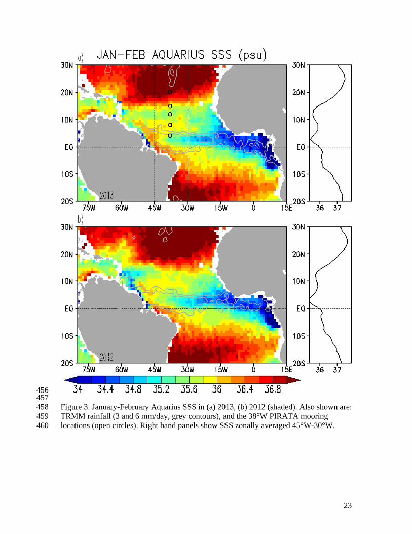
456 457 458 459 460
Figure 3. January-February Aquarius SSS in (a) 2013, (b) 2012 (shaded). Also shown are: TRMM rainfall (3 and 6 mm/day, grey contours), and the 38°W PIRATA mooring locations (open circles). Right hand panels show SSS zonally averaged 45°W-30°W.
23
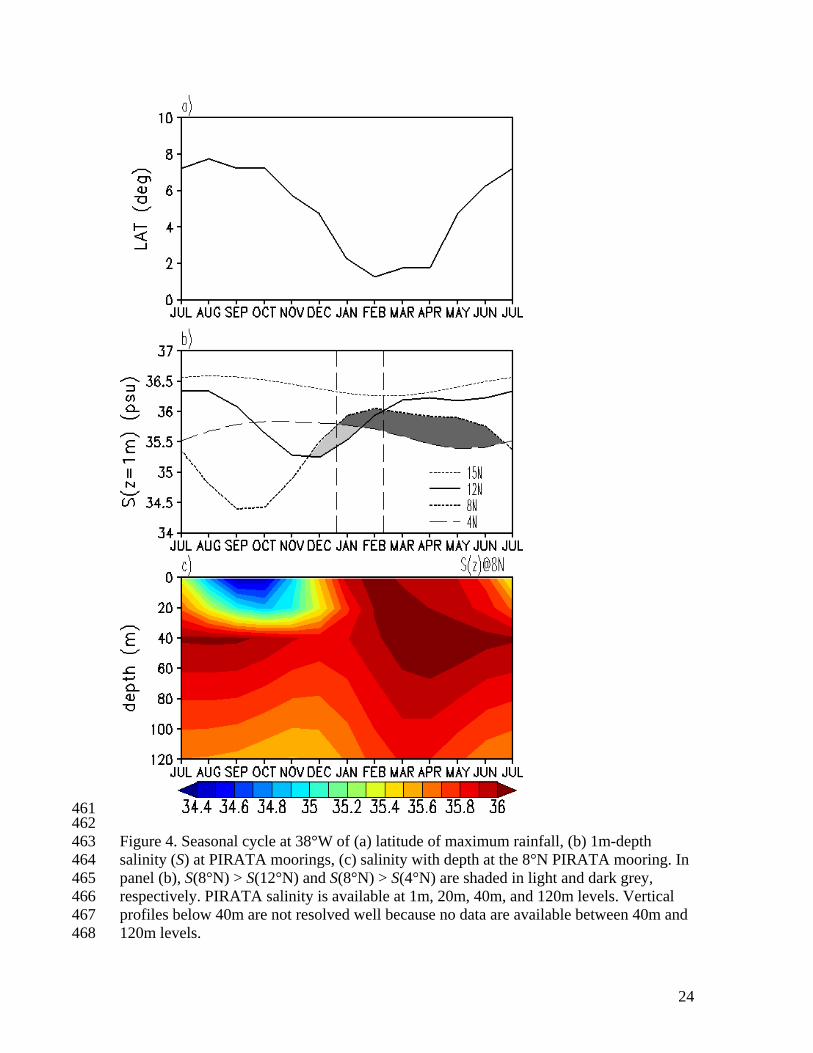
461 462 463 464 465 466 467 468
Figure 4. Seasonal cycle at 38°W of (a) latitude of maximum rainfall, (b) 1m-depth salinity (S) at PIRATA moorings, (c) salinity with depth at the 8°N PIRATA mooring. In panel (b), S(8°N) > S(12°N) and S(8°N) > S(4°N) are shaded in light and dark grey, respectively. PIRATA salinity is available at 1m, 20m, 40m, and 120m levels. Vertical profiles below 40m are not resolved well because no data are available between 40m and 120m levels.
24

469 470 471 472 473
Figure 5. AQUARIUS SSS (psu, shaded) and TRMM rainfall > 3 mm/day (CI=3mm/day) averaged 45°W-30°W. Slope line corresponds to 4 cm/s northward propagation.
25

474 475 476 477 478 479
Figure 6. January simulated SSS (model year 67, psu, shaded), surface currents (arrows, westward white, eastward red), and net surface freshwater flux (P-E, 2.5mm/day, 5mm/day contours). Two boxes: a northern box (47°W-35°W, 10°N-15°N) and an NECC box (47°W-35°W, 4°N-9°N) are selected for salt budget analysis in Fig.7.
26

480 481 482
Figure 7. Mixed layer salt budget spatially averaged over the northern box (see Fig. 6): (a) box averaged salinity (psu) and mixed layer depth ( H ); (b) salt tendency (TEND) and the sum of surface salt flux (SSF), meridional advection by monthly currents (MADV), and vertical salt diffusion across the mixed layer base (VDIF); (c) budget terms shown separately including the horizontal eddy salt flux (HEDDY) by intra-month oscillations.
483 484 485 486
27

487 488 489
Figure 8. Mixed layer salt budget spatially averaged over the NECC box (see Fig. 6): (a) horizontally averaged salinity (psu) and mixed layer depth ( H ); (b) salt tendency (TEND) and horizontal advection by monthly currents (HADV); (c) budget terms shown separately including the 3-D eddy salt flux (EDDY) by intra-month oscillations. Note that temporal changes of horizontally averaged salinity and
490 491 492
H in (a) don’t match in this high gradient region.
493 494
28

495 496 497 498 499
Figure 9. January-February SSS climatology from (a) Dessier and Donguy (1994), (b) WOA09, and (c) based on ARGO float observations. Right panels show SSS averaged 45°W-30°W.
29