898 IEEE TRANSACTIONS ON GEOSCIENCE AND REMOTE …bioucas/files/ieeegrsVca04.pdf · 898 IEEE TRANSACTIONS ON GEOSCIENCE AND REMOTE SENSING, VOL. 43, NO. 4, APRIL 2005 Vertex Component

898 IEEE TRANSACTIONS ON GEOSCIENCE AND REMOTE SENSING, VOL. 43, NO. 4, APRIL 2005

Vertex Component Analysis: A Fast Algorithm toUnmix Hyperspectral Data

José M. P. Nascimento, Student Member, IEEE, and José M. Bioucas Dias, Member, IEEE

Abstract—Given a set of mixed spectral (multispectral or hy-perspectral) vectors, linear spectral mixture analysis, or linearunmixing, aims at estimating the number of reference substances,also called endmembers, their spectral signatures, and theirabundance fractions. This paper presents a new method forunsupervised endmember extraction from hyperspectral data,termed vertex component analysis (VCA). The algorithm exploitstwo facts: 1) the endmembers are the vertices of a simplex and 2)the affine transformation of a simplex is also a simplex. In a seriesof experiments using simulated and real data, the VCA algorithmcompetes with state-of-the-art methods, with a computationalcomplexity between one and two orders of magnitude lower thanthe best available method.

Index Terms—Linear unmixing, simplex, spectral mixturemodel, unmixing hypespectral data, unsupervised endmemberextraction, vertex component analysis (VCA).

I. INTRODUCTION

HYPERSPECTRAL remote sensing exploits the electro-magnetic (EM) scattering patterns of different materials at

specific wavelengths [1], [2]. Hyperspectral sensors have beendeveloped to sample the scattered portion of the EM spectrumextending from the visible region through the near-infrared andmidinfrared, in hundreds of narrow contiguous bands [3], [4].The number and variety of potential civilian and military appli-cations of hyperspectral remote sensing is enormous [5], [6].

Very often, the resolution cell corresponding to a single pixelin an image contains several substances (endmembers) [3]. Inthis situation, the scattered energy is a mixing of the endmemberspectra. A challenging task underlying many hyperspectral im-agery applications is then decomposing a mixed pixel into a col-lection of reflectance spectra, called endmember signatures, andthe corresponding abundance fractions [7]–[9].

Depending on the mixing scales at each pixel, the observedmixture is either linear or nonlinear [10], [11]. A linear mixingmodel holds approximately when the mixing scale is macro-scopic [12] and there is negligible interaction among distinctendmembers [2], [13]. If, however, the mixing scale is micro-scopic (or intimate mixtures) [14], [15] and the incident solar

Manuscript received January 6, 2004; revised December 21, 2004. This workwas supported in part by the Fundação para a Ciência e Tecnologia under theProjects POSI/34071/CPS/2000 and PDCTE/CPS/49967/2003 and in part bythe Departamento de Engenharia de Electrónica e Telecomunicações e de Com-putadores of the Instituto Superior de Engenharia de Lisboa.

J. M. P. Nascimento is with the Instituto Superior de Engenharia de Lisboaand the Instituto de Telecomunicações, 1949-001 Lisbon, Portugal (e-mail:[email protected]).

J. M. Bioucas Dias is with the Instituto de Telecomunicações and the InstitutoSuperiror Técnico, 1949-001 Lisbon, Portugal (e-mail: [email protected]).

Digital Object Identifier 10.1109/TGRS.2005.844293

radiation is scattered by the scene through multiple bounces in-volving several endmembers [16], the linear model is no longeraccurate.

Linear spectral unmixing has been intensively researchedin the last years [8], [9], [11], [17]–[20]. It considers that amixed pixel is a linear combination of endmember signaturesweighted by the correspondent abundance fractions. Underthis model, and assuming that the number of substances andtheir reflectance spectra are known, hyperspectral unmixing isa linear problem for which many solutions have been proposed(e.g., maximum-likelihood estimation [7], spectral signaturematching [21], spectral angle mapper [22], subspace projectionmethods [23], [24], and constrained least squares [25]).

In most cases, the number of substances and their reflectancesare not known and, then, hyperspectral unmixing falls into theclass of blind source separation problems [26]. independentcomponent analysis (ICA) has recently been proposed as a toolto blindly unmix hyperspectral data [27]–[30]. ICA is based onthe assumption of mutually independent sources (abundancefractions), which is not the case of hyperspectral data, sincethe sum of abundance fractions is constant, implying statisticaldependence among them. This dependence compromises ICAapplicability to hyperspectral images as shown in [20] and[31]. In fact, ICA finds the endmember signatures by mul-tiplying the spectral vectors with an unmixing matrix whichminimizes the mutual information among channels. If sourcesare independent, ICA provides the correct unmixing, since theminimum of the mutual information corresponds to and onlyto independent sources. This is no longer true for dependentfractional abundances. Nevertheless, some endmembers may beapproximately unmixed. These aspects are addressed in [31].

Under the linear mixing model, the observations from a sceneare in a simplex whose vertices correspond to the endmembers.Several approaches [32]–[34] have exploited this geometric fea-ture of hyperspectral mixtures [33].The minimum volume transform (MVT) algorithm [34] deter-mines the simplex of minimum volume containing the data.The method presented in [35] is also of MVT type, but by in-troducing the notion of bundles, it takes into account the end-member variability usually present in hyperspectral mixtures.

The MVT type approaches are complex from the compu-tational point of view. Usually, these algorithms first find theconvex hull defined by the observed data and then fit a minimumvolume simplex to it. For example, the gift wrapping algorithm[36] computes the convex hull of data points in a -dimen-sional space with a computational complexity of ,where is the highest integer lower or equal than , and isthe number of samples. The complexity of the method presented

0196-2892/$20.00 © 2005 IEEE

NASCIMENTO AND DIAS: VERTEX COMPONENT ANALYSIS 899

in [35] is even higher, since the temperature of the simulated an-nealing algorithm therein used shall follow a law [37] toassure convergence (in probability) to the desired solution.

Aiming at a lower computational complexity, some al-gorithms such as the pixel purity index (PPI) [33] and theN-FINDR [38] still find the minimum volume simplex con-taining the data cloud, but they assume the presence in the dataof at least one pure pixel of each endmember. This is a strongrequisite that may not hold in some datasets. In any case, thesealgorithms find the set of most pure pixels in the data.

The PPI algorithm uses the minimum-noise fraction (MNF)[39] as a preprocessing step to reduce dimensionality and toimprove the signal-to-noise ratio (SNR). The algorithm thenprojects every spectral vector onto skewers (large number ofrandom vectors) [33], [40], [41]. The points corresponding toextremes, for each skewer direction, are stored. A cumulativeaccount records the number of times each pixel (i.e., a givenspectral vector) is found to be an extreme. The pixels with thehighest scores are the purest ones.

The N-FINDR algorithm [38] is based on the fact that inspectral dimensions, the -volume defined by a simplex formedby the purest pixels is larger than any other volume defined byany other combination of pixels. This algorithm finds the set ofpixels defining the largest volume by inflating a simplex insidethe data.

ORASIS [42], [43] is a hyperspectral framework developedby the Naval Research Laboratory consisting of several algo-rithms organized in six modules: exemplar selector, adaptativelearner, demixer, knowledge base/spectral library, and spatialpostprocessor. The first step consists in flat fielding the spectra.Next, the exemplar selection module is used to select spectralvectors that best represent the smaller convex cone containingthe data. The other pixels are rejected when the spectral angledistance is less than a given threshold. The procedure finds thebasis for a subspace of a lower dimension using a modifiedGram-Schmidt orthogonalization. The selected vectors are thenprojected onto this subspace, and a simplex is found by an MVTprocess. ORASIS is oriented to real-time target detection fromuncrewed air vehicles using hyperspectral data [44].

In this paper we introduce the vertex component analysis(VCA) algorithm to unmix linear mixtures of endmemberspectra. The algorithm is unsupervised and exploits two facts:1) the endmembers are the vertices of a simplex and 2) theaffine transformation of a simplex is also a simplex. It workswith unprojected and with projected data. As PPI and N-FINDRalgorithms, VCA also assumes the presence of pure pixels inthe data. The algorithm iteratively projects data onto a directionorthogonal to the subspace spanned by the endmembers alreadydetermined. The new endmember signature corresponds tothe extreme of the projection. The algorithm iterates until allendmembers are exhausted. VCA performs much better thanPPI and better than or comparable to N-FINDR; yet it hasa computational complexity between one and two orders ofmagnitude lower than N-FINDR.

The paper is structured as follows. Section II describes thegeometric fundamentals of the proposed method. Sections IIIand IV evaluate the proposed algorithm using simulated and real

data, respectively. Section V ends the paper by presenting someconcluding remarks.

II. VERTEX COMPONENT ANALYSIS ALGORITHM

Assuming the linear mixing scenario, each observed spectralvector is given by

(1)

where is an -vector ( is the number of bands),is the mixing matrix ( denotes the

th endmember signature and is the number of endmemberspresent in the covered area), ( is a scale factormodeling illumination variability due to surface topography),

is the abundance vector containingthe fractions of each endmember (the notation stands forvector transposed) and models system additive noise.

Owing to physical constraints [19], abundance fractions arenonnegative and satisfy the so-called positivity con-straint , where is a vector of ones. Each pixelcan be viewed as a vector in an -dimensional Euclidean space,where each channel is assigned to one axis of space. Since theset is a simplex, then the set

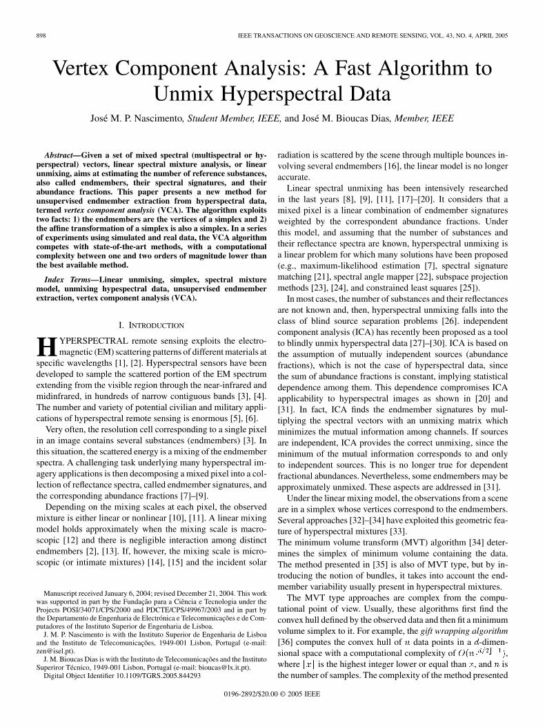
is also a simplex.However, even assuming , the observed vector set be-longs tothat is a convex cone, owing to scale factor . Fig. 1(a) illus-trates a simplex and a cone, projected on a two-dimensional sub-space, defined by a mixture of three endmembers. The simplexboundary is a triangle whose vertices correspond to the end-members shown in Fig. 2. Small and medium dots are simulatedmixed spectra belonging to the simplex and to thecone , respectively.

The projective projection of the convex cone onto a prop-erly chosen hyperplane is a simplex with vertices correspondingto the vertices of the simplex . This is illustrated in Fig. 1(b).The simplex isthe projective projection of the convex cone onto the plane

, where the choice of assures that there is no ob-served vectors orthogonal to it.

After identifying , the VCA algorithm iteratively projectsdata onto a direction orthogonal to the subspace spanned by theendmembers already determined. The new endmember signa-ture corresponds to the extreme of the projection. Fig. 1(b) il-lustrates the two iterations of VCA algorithm applied to the sim-plex defined by the mixture of two endmembers. In the firstiteration, data are projected onto the first direction . The ex-treme of the projection corresponds to endmember . In thenext iteration, endmember is found by projecting data ontodirection , which is orthogonal to . The algorithm iteratesuntil the number of endmembers is exhausted.

A. Dimensionality Reduction

Under the linear observation model, spectral vectors are in asubspace of dimension . If , it is worthy to project theobserved spectral vectors onto the subspace signal. This leads


(a)

(b)

Fig. 1. (a) Two-dimensional scatterplot of mixtures of the three endmembersshown in Fig. 2. Circles denote pure materials. (b) Illustration of the VCAalgorithm.

Fig. 2. Reflectances of carnallite, ammonioalunite, and biotite.

to significant savings in computational complexity and to SNRimprovements.

Principal component analysis (PCA) [45], maximum-noisefraction (MNF) [46], and singular value decomposition (SVD)[47] are three well-known projection techniques widely used inremote sensing. PCA, also known as Karhunen–Loéve trans-form, seeks the projection that best represents data in a least-squares sense; MNF seeks the projection that optimizes SNR;and SVD provides the projection that best represents data in themaximum-power sense. PCA and MNF are equal in the case

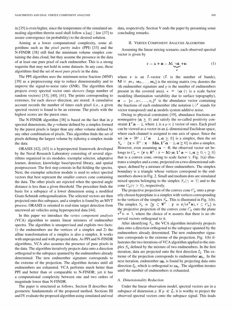
Fig. 3. Scatterplot (bands � = 827 nm and � = 1780 nm) of the threeendmembers mixture. (a) Unprojected data. (b) Projected data using SVD. Solidand dashed lines represent, respectively, simplexes computed from original andestimated endmembers (using VCA).

of white noise. SVD and PCA are also equal in the case ofzero-mean data.

As discussed before, in the absence of noise, observed vec-tors lie in a convex cone contained in a subspace ofdimension . The VCA algorithm starts by identifying bySVD and then projects points in onto a simplex by com-puting [see Fig. 1(b)]. This simplex is containedin an affine set of dimension . We note that the rational un-derlying the VCA algorithm is still valid if the observed datasetis projected onto any subspace of dimension , for

, i.e., the projection of the cone onto followedby a projective projection is also a simplex with the same ver-tices. Of course, the SNR decreases as increases.

For illustration purposes, a simulated scene was gener-ated according to (1). Three spectral signatures (A—bi-otite, B—carnallite, and C—ammonioalunite) were selectedfrom the U.S. Geological Survey (USGS) digital spectrallibrary [48] (see Fig. 2); the abundance fractions follow aDirichlet distribution; parameter is set to 1; and the noiseis zero-mean white Gaussian with covariance matrix ,where is the identity matrix and leading toa SNR dB. Fig. 3(a)presents a scatterplot of the simulated spectral mixtures withoutprojection (bands nm and nm). Twotriangles are also plotted whose vertices represent the true end-members (solid line) and the estimated endmembers (dashedline) by the VCA algorithm, respectively. Fig. 3(b) presents ascatterplot (same bands) of projected data onto the estimatedaffine set of dimension two inferred by SVD. Noise is clearlyreduced, leading to a visible improvement on the VCA results.

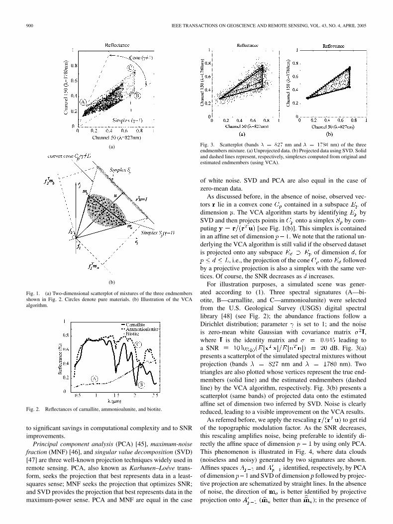
As referred before, we apply the rescaling to get ridof the topographic modulation factor. As the SNR decreases,this rescaling amplifies noise, being preferable to identify di-rectly the affine space of dimension by using only PCA.This phenomenon is illustrated in Fig. 4, where data clouds(noiseless and noisy) generated by two signatures are shown.Affines spaces and identified, respectively, by PCAof dimension and SVD of dimension followed by projec-tive projection are schematized by straight lines. In the absenceof noise, the direction of is better identified by projectiveprojection onto ( better than ); in the presence of


strong noise, the direction of is better identified by orthog-onal projection onto ( better than ). As a conclu-sion, when the SNR is higher than a given threshold SNR ,data is projected onto followed by the rescaling ;otherwise data are projected onto . Based on experimentalresults, we propose the threshold SNR dB.Since for zero-mean white noise SNR , thenwe conclude that at SNR , , i.e., theSNR corresponds to the fixed value of the SNR mea-sured with respect to the signal subspace.

B. VCA Algorithm

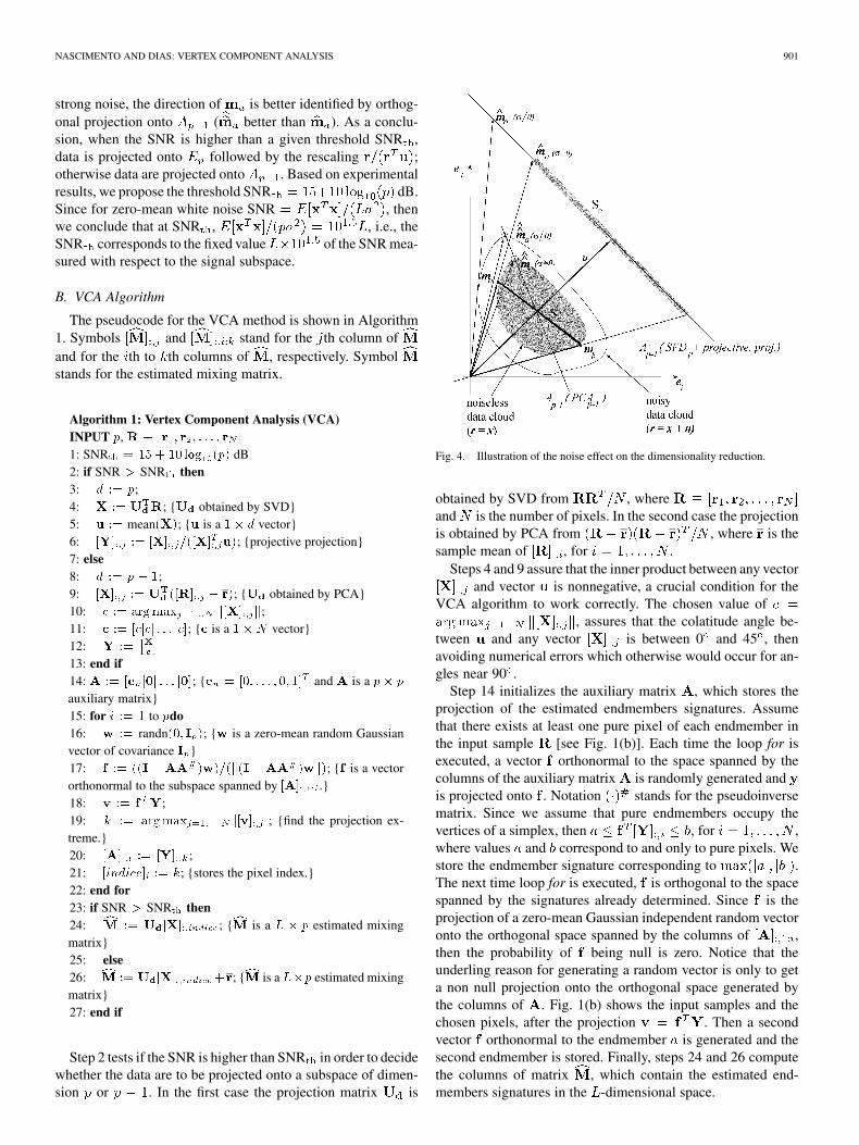
The pseudocode for the VCA method is shown in Algorithm1. Symbols and stand for the th column ofand for the th to th columns of , respectively. Symbolstands for the estimated mixing matrix.

Algorithm 1: Vertex Component Analysis (VCA)INPUT p, R � [r1; r2; . . . ; rN ]

1: SNRth = 15 + 10 log10(p) dB2: if SNR > SNRth then3: d := p;4: X := U

T

dR; {Ud obtained by SVD}5: u := mean(X); {u is a 1 � d vector}6: [Y]:;j := [X]:;j=([X]T:;ju); {projective projection}7: else8: d := p � 1;9: [X]:;j := U

T

d ([R]:;j � r); {Ud obtained by PCA}10: c := argmaxj=1...N k[X]:;jk;11: c := [cjcj . . . jc]; {c is a 1� N vector}12: Y := X

c

13: end if14: A := [euj0j . . . j0]; {eu = [0; . . . ; 0; 1]T and A is a p � p

auxiliary matrix}15: for i := 1 to pdo16: w := randn(0; Ip); {w is a zero-mean random Gaussianvector of covariance Ip}17: f := ((I�AA

#)w)=(k(I�AA#)wk); {f is a vector

orthonormal to the subspace spanned by [A]:;1:i.}18: v := f

TY;

19: k := argmaxj=1;...;N j[v]:;j j; {find the projection ex-treme.}20: [A]:;i := [Y]:;k;21: [indice]i := k; {stores the pixel index.}22: end for23: if SNR > SNRth then24: M := Ud[X]:;indice; {M is a L � p estimated mixingmatrix}25: else26: M := Ud[X]:;indice+r; {M is a L�p estimated mixingmatrix}27: end if

Step 2 tests if the SNR is higher than SNR in order to decidewhether the data are to be projected onto a subspace of dimen-sion or . In the first case the projection matrix is

Fig. 4. Illustration of the noise effect on the dimensionality reduction.

obtained by SVD from , whereand is the number of pixels. In the second case the projectionis obtained by PCA from , where is thesample mean of , for .

Steps 4 and 9 assure that the inner product between any vectorand vector is nonnegative, a crucial condition for the

VCA algorithm to work correctly. The chosen value of, assures that the colatitude angle be-

tween and any vector is between 0 and 45 , thenavoiding numerical errors which otherwise would occur for an-gles near 90 .

Step 14 initializes the auxiliary matrix , which stores theprojection of the estimated endmembers signatures. Assumethat there exists at least one pure pixel of each endmember inthe input sample [see Fig. 1(b)]. Each time the loop for isexecuted, a vector orthonormal to the space spanned by thecolumns of the auxiliary matrix is randomly generated andis projected onto . Notation stands for the pseudoinversematrix. Since we assume that pure endmembers occupy thevertices of a simplex, then , for ,where values and correspond to and only to pure pixels. Westore the endmember signature corresponding to .The next time loop for is executed, is orthogonal to the spacespanned by the signatures already determined. Since is theprojection of a zero-mean Gaussian independent random vectoronto the orthogonal space spanned by the columns of ,then the probability of being null is zero. Notice that theunderling reason for generating a random vector is only to geta non null projection onto the orthogonal space generated bythe columns of . Fig. 1(b) shows the input samples and thechosen pixels, after the projection . Then a secondvector orthonormal to the endmember is generated and thesecond endmember is stored. Finally, steps 24 and 26 computethe columns of matrix , which contain the estimated end-members signatures in the -dimensional space.


III. EVALUATION OF THE VCA ALGORITHM

In this section, we compare VCA, PPI, and N-FINDR al-gorithms. N-FINDR and PPI were coded accordingly to [38]and [33], respectively. Regarding PPI, the number of skewersmust be large [39], [40], [49]–[51]. Based on Monte Carloruns, we concluded that the minimum number of skewersbeyond which there is no unmixing improvements is about1000. All experiments are based on simulated scenes fromwhich we know the signature endmembers and their frac-tional abundances. Estimated endmembers are the columns of

. We also compare estimated abun-dance fractions given by , ( standsfor pseudoinverse of ) with the true abundance fractions.

To evaluate the performance of the three algorithms,we compute vectors of angles and

with1

(2)

(3)

where is the angle between vectors and ( th end-member signature estimate) and is the angle between vectors

and (vectors of formed by the th lines of ma-trices and , respectively). The symmetricKullback distance [52], a relative entropy-based distance, is an-other error measure used to compare similarity between signa-tures, namely under the name spectral information divergence(SID) [53]. SID is defined by

SID (4)

where is the relative entropy of with respect togiven by

(5)

and and .Based on , , and SID SID

SID , we estimate the following rms error distances:

(6)

(7)

(8)

where denotes the expectation operator. The first two quan-tities measure distances between and , for ;the third is similar to the first, but for the estimated abundance

1Notation hx;yi stands for the inner product x y.

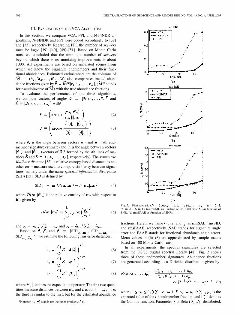
Fig. 5. First scenario (N = 1000, p = 3, L = 224, � = � = � = 1=3,� = 20, � = 1). (a) rmsSID as function of SNR. (b) rmsSAE as function ofSNR. (c) rmsFAAE as function of SNRs.

fractions. Herein we name , , and as rmsSAE, rmsSID,and rmsFAAE, respectively (SAE stands for signature angleerror and FAAE stands for fractional abundance angle error).Mean values in (6)–(8) are approximated by sample meansbased on 100 Monte Carlo runs.

In all experiments, the spectral signatures are selectedfrom the USGS digital spectral library [48]. Fig. 2 showsthree of these endmember signatures. Abundance fractionsare generated according to a Dirichlet distribution given by

(9)

where , , is theexpected value of the th endmember fraction, and denotesthe Gamma function. Parameter is Beta distributed,


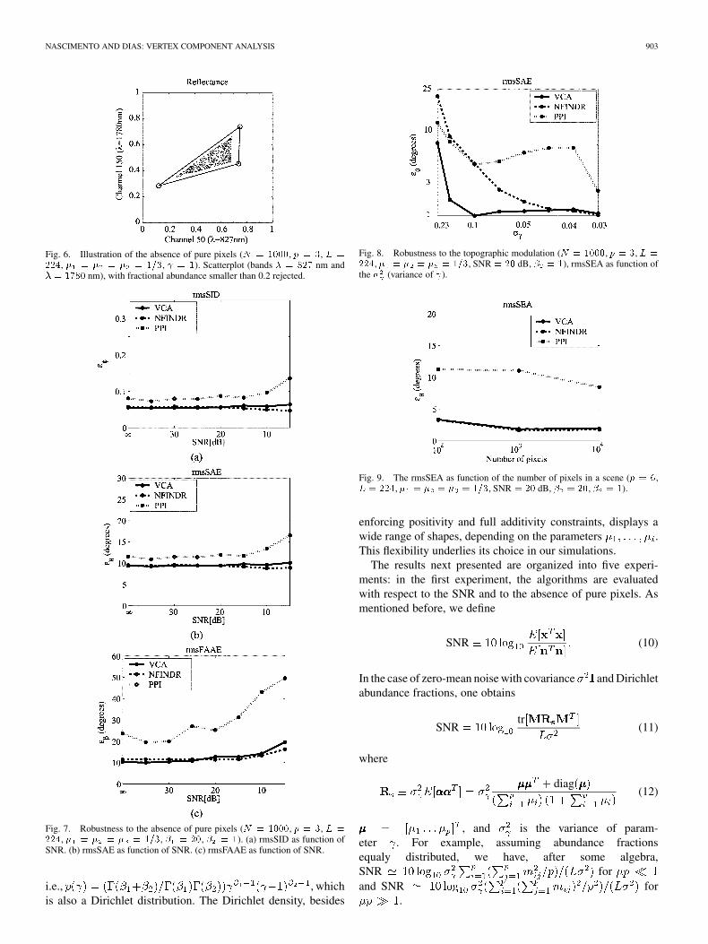
Fig. 6. Illustration of the absence of pure pixels (N = 1000, p = 3, L =

224, � = � = � = 1=3, = 1). Scatterplot (bands � = 827 nm and� = 1780 nm), with fractional abundance smaller than 0.2 rejected.

Fig. 7. Robustness to the absence of pure pixels (N = 1000, p = 3, L =

224, � = � = � = 1=3, � = 20, � = 1). (a) rmsSID as function ofSNR. (b) rmsSAE as function of SNR. (c) rmsFAAE as function of SNR.

i.e., , whichis also a Dirichlet distribution. The Dirichlet density, besides

Fig. 8. Robustness to the topographic modulation (N = 1000, p = 3, L =

224, � = � = � = 1=3, SNR = 20 dB, � = 1), rmsSEA as function ofthe � (variance of ).

Fig. 9. The rmsSEA as function of the number of pixels in a scene (p = 6,L = 224, � = � = � = 1=3, SNR = 20 dB, � = 20, � = 1).

enforcing positivity and full additivity constraints, displays awide range of shapes, depending on the parameters .This flexibility underlies its choice in our simulations.

The results next presented are organized into five experi-ments: in the first experiment, the algorithms are evaluatedwith respect to the SNR and to the absence of pure pixels. Asmentioned before, we define

SNR (10)

In the case of zero-mean noise with covariance and Dirichletabundance fractions, one obtains

SNRtr

(11)

where

diag(12)

, and is the variance of param-eter . For example, assuming abundance fractionsequaly distributed, we have, after some algebra,SNR forand SNR for

.


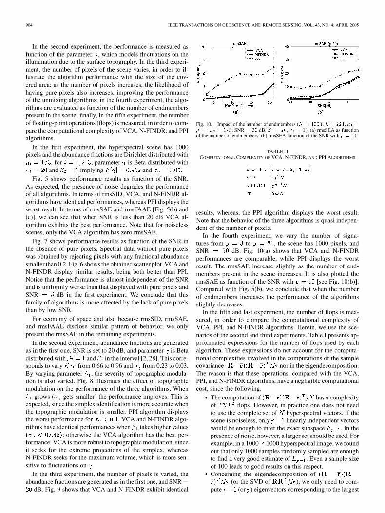
In the second experiment, the performance is measured asfunction of the parameter , which models fluctuations on theillumination due to the surface topography. In the third experi-ment, the number of pixels of the scene varies, in order to il-lustrate the algorithm performance with the size of the cov-ered area: as the number of pixels increases, the likelihood ofhaving pure pixels also increases, improving the performanceof the unmixing algorithms; in the fourth experiment, the algo-rithms are evaluated as function of the number of endmemberspresent in the scene; finally, in the fifth experiment, the numberof floating-point operations (flops) is measured, in order to com-pare the computational complexity of VCA, N-FINDR, and PPIalgorithms.

In the first experiment, the hyperspectral scene has 1000pixels and the abundance fractions are Dirichlet distributed with

, for ; parameter is Beta distributed withand implying and .

Fig. 5 shows performance results as function of the SNR.As expected, the presence of noise degrades the performanceof all algorithms. In terms of rmsSID, VCA, and N-FINDR al-gorithms have identical performances, whereas PPI displays theworst result. In terms of rmsSAE and rmsFAAE [Fig. 5(b) and(c)], we can see that when SNR is less than 20 dB VCA al-gorithm exhibits the best performance. Note that for noiselessscenes, only the VCA algorithm has zero rmsSAE.

Fig. 7 shows performance results as function of the SNR inthe absence of pure pixels. Spectral data without pure pixelswas obtained by rejecting pixels with any fractional abundancesmaller than 0.2. Fig. 6 shows the obtained scatter plot. VCA andN-FINDR display similar results, being both better than PPI.Notice that the performance is almost independent of the SNRand is uniformly worse than that displayed with pure pixels andSNR dB in the first experiment. We conclude that thisfamily of algorithms is more affected by the lack of pure pixelsthan by low SNR.

For economy of space and also because rmsSID, rmsSAE,and rmsFAAE disclose similar pattern of behavior, we onlypresent the rmsSAE in the remaining experiments.

In the second experiment, abundance fractions are generatedas in the first one, SNR is set to 20 dB, and parameter is Betadistributed with and in the interval [2, 28]. This corre-sponds to vary from 0.66 to 0.96 and from 0.23 to 0.03.By varying parameter , the severity of topographic modula-tion is also varied. Fig. 8 illustrates the effect of topographicmodulation on the performance of the three algorithms. When

grows ( gets smaller) the performance improves. This isexpected, since the simplex identification is more accurate whenthe topographic modulation is smaller. PPI algorithm displaysthe worst performance for . VCA and N-FINDR algo-rithms have identical performances when takes higher values

; otherwise the VCA algorithm has the best per-formance. VCA is more robust to topographic modulation, sinceit seeks for the extreme projections of the simplex, whereasN-FINDR seeks for the maximum volume, which is more sen-sitive to fluctuations on .

In the third experiment, the number of pixels is varied, theabundance fractions are generated as in the first one, and SNR

dB. Fig. 9 shows that VCA and N-FINDR exhibit identical

Fig. 10. Impact of the number of endmembers (N = 1000,L = 224, � =

� = � = 1=3, SNR = 30 dB, � = 20, � = 1). (a) rmsSEA as functionof the number of endmembers. (b) rmsSEA function of the SNR with p = 10.

TABLE ICOMPUTATIONAL COMPLEXITY OF VCA, N-FINDR, AND PPI ALGORITHMS

results, whereas, the PPI algorithm displays the worst result.Note that the behavior of the three algorithms is quasi indepen-dent of the number of pixels.

In the fourth experiment, we vary the number of signa-tures from to , the scene has 1000 pixels, andSNR dB. Fig. 10(a) shows that VCA and N-FINDRperformances are comparable, while PPI displays the worstresult. The rmsSAE increase slightly as the number of end-members present in the scene increases. It is also plotted thermsSAE as function of the SNR with [see Fig. 10(b)].Compared with Fig. 5(b), we conclude that when the numberof endmembers increases the performance of the algorithmsslightly decreases.

In the fifth and last experiment, the number of flops is mea-sured, in order to compare the computational complexity ofVCA, PPI, and N-FINDR algorithms. Herein, we use the sce-narios of the second and third experiments. Table I presents ap-proximated expressions for the number of flops used by eachalgorithm. These expressions do not account for the computa-tional complexities involved in the computations of the samplecovariance nor in the eigendecomposition.The reason is that these operations, compared with the VCA,PPI, and N-FINDR algorithms, have a negligible computationalcost, since the following.

• The computation of has a complexityof flops. However, in practice one does not needto use the complete set of hyperspectral vectors. If thescene is noiseless, only linearly independent vectorswould be enough to infer the exact subspace . In thepresence of noise, however, a larger set should be used. Forexample, in a 1000 1000 hyperspectral image, we foundout that only 1000 samples randomly sampled are enoughto find a very good estimate of . Even a sample sizeof 100 leads to good results on this respect.

• Concerning the eigendecomposition of(or the SVD of ), we only need to com-

pute (or ) eigenvectors corresponding to the largest


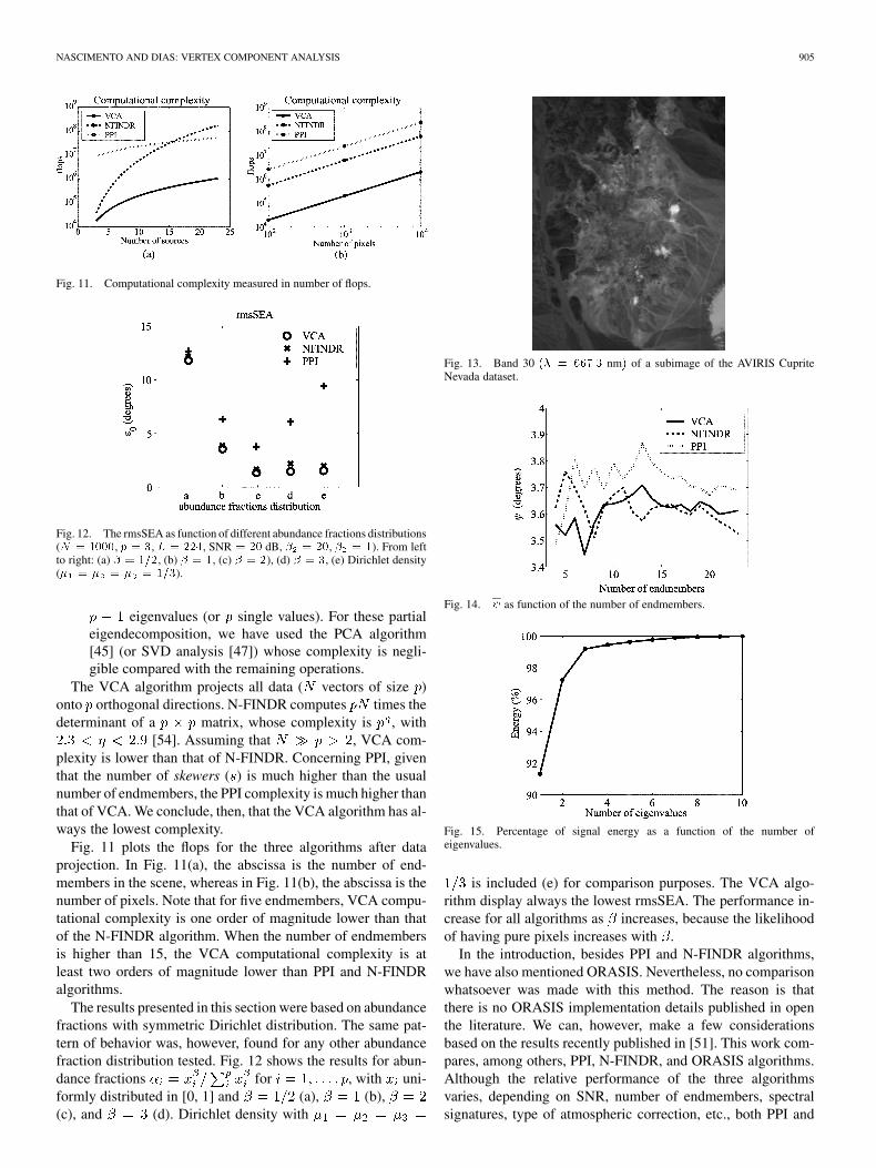
Fig. 11. Computational complexity measured in number of flops.

Fig. 12. The rmsSEA as function of different abundance fractions distributions(N = 1000, p = 3, L = 224, SNR = 20 dB, � = 20, � = 1). From leftto right: (a) � = 1=2, (b) � = 1, (c) � = 2), (d) � = 3, (e) Dirichlet density(� = � = � = 1=3).

eigenvalues (or single values). For these partialeigendecomposition, we have used the PCA algorithm[45] (or SVD analysis [47]) whose complexity is negli-gible compared with the remaining operations.

The VCA algorithm projects all data ( vectors of size )onto orthogonal directions. N-FINDR computes times thedeterminant of a matrix, whose complexity is , with

[54]. Assuming that , VCA com-plexity is lower than that of N-FINDR. Concerning PPI, giventhat the number of skewers ( ) is much higher than the usualnumber of endmembers, the PPI complexity is much higher thanthat of VCA. We conclude, then, that the VCA algorithm has al-ways the lowest complexity.

Fig. 11 plots the flops for the three algorithms after dataprojection. In Fig. 11(a), the abscissa is the number of end-members in the scene, whereas in Fig. 11(b), the abscissa is thenumber of pixels. Note that for five endmembers, VCA compu-tational complexity is one order of magnitude lower than thatof the N-FINDR algorithm. When the number of endmembersis higher than 15, the VCA computational complexity is atleast two orders of magnitude lower than PPI and N-FINDRalgorithms.

The results presented in this section were based on abundancefractions with symmetric Dirichlet distribution. The same pat-tern of behavior was, however, found for any other abundancefraction distribution tested. Fig. 12 shows the results for abun-dance fractions for , with uni-formly distributed in [0, 1] and (a), (b),(c), and (d). Dirichlet density with

Fig. 13. Band 30 (� = 667:3 nm) of a subimage of the AVIRIS CupriteNevada dataset.

Fig. 14. as function of the number of endmembers.

Fig. 15. Percentage of signal energy as a function of the number ofeigenvalues.

is included (e) for comparison purposes. The VCA algo-rithm display always the lowest rmsSEA. The performance in-crease for all algorithms as increases, because the likelihoodof having pure pixels increases with .

In the introduction, besides PPI and N-FINDR algorithms,we have also mentioned ORASIS. Nevertheless, no comparisonwhatsoever was made with this method. The reason is thatthere is no ORASIS implementation details published in openthe literature. We can, however, make a few considerationsbased on the results recently published in [51]. This work com-pares, among others, PPI, N-FINDR, and ORASIS algorithms.Although the relative performance of the three algorithmsvaries, depending on SNR, number of endmembers, spectralsignatures, type of atmospheric correction, etc., both PPI and


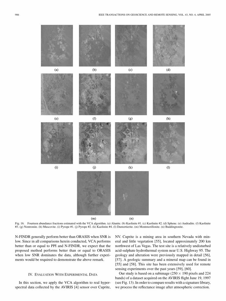
Fig. 16. Fourteen abundance fractions estimated with the VCA algorithm. (a) Alunite. (b) Kaolinite #1. (c) Kaolinite #2. (d) Sphene. (e) Andradite. (f) Kaolinite#3. (g) Nontronite. (h) Muscovite. (i) Pyrope #1. (j) Pyrope #2. (k) Kaolinite #4. (l) Dumortierite. (m) Montmorillonite. (n) Buddingtonite.

N-FINDR generally perform better than ORASIS when SNR islow. Since in all comparisons herein conducted, VCA performsbetter than or equal to PPI and N-FINDR, we expect that theproposed method performs better than or equal to ORASISwhen low SNR dominates the data, although further experi-ments would be required to demonstrate the above remark.

IV. EVALUATION WITH EXPERIMENTAL DATA

In this section, we apply the VCA algorithm to real hyper-spectral data collected by the AVIRIS [4] sensor over Cuprite,

NV. Cuprite is a mining area in southern Nevada with min-eral and little vegetation [55], located approximately 200 kmnorthwest of Las Vegas. The test site is a relatively undisturbedacid-sulphate hydrothermal system near U.S. Highway 95. Thegeology and alteration were previously mapped in detail [56],[57]. A geologic summary and a mineral map can be found in[55] and [58]. This site has been extensively used for remotesensing experiments over the past years [59], [60].

Our study is based on a subimage (250 190 pixels and 224bands) of a dataset acquired on the AVIRIS flight June 19, 1997(see Fig. 13). In order to compare results with a signature library,we process the reflectance image after atmospheric correction.


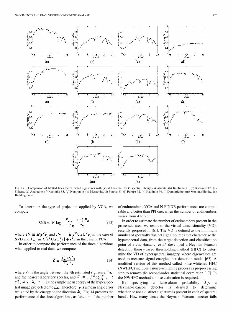
Fig. 17. Comparison of (dotted line) the extracted signatures with (solid line) the USGS spectral library. (a) Alunite. (b) Kaolinite #1. (c) Kaolinite #2. (d)Sphene. (e) Andradite. (f) Kaolinite #3. (g) Nontronite. (h) Muscovite. (i) Pyrope #1. (j) Pyrope #2. (k) Kaolinite #4. (l) Dumortierite. (m) Montmorillonite. (n)Buddingtonite.

To determine the type of projection applied by VCA, wecompute

SNR (13)

where and in the case ofSVD and in the case of PCA.

In order to compare the performance of the three algorithmswhen applied to real data, we compute

(14)

where is the angle between the th estimated signature, ,and the nearest laboratory spectra, and

, is the sample mean energy of the hyperspec-tral image projected onto . Therefore, is a mean angle errorweighted by the energy on the direction . Fig. 14 presents theperformance of the three algorithms, as function of the number

of endmembers. VCA and N-FINDR performances are compa-rable and better than PPI one, when the number of endmembersvaries from 4 to 23.

In order to estimate the number of endmembers present in theprocessed area, we resort to the virtual dimensionality (VD),recently proposed in [61]. The VD is defined as the minimumnumber of spectrally distinct signal sources that characterize thehyperspectral data, from the target detection and classificationpoint of view. Harsanyi et al. developed a Neyman–Pearsondetection theory-based thresholding method (HFC) to deter-mine the VD of hyperspectral imagery, where eigenvalues areused to measure signal energies in a detection model [62]. Amodified version of this method called noise-whitened HFC(NWHFC) includes a noise-whitening process as preprocessingstep to remove the second-order statistical correlation [17]. Inthe NWHFC method a noise estimation is required.

By specifying a false-alarm probability , aNeyman–Pearson detector is derived to determinewhether or not a distinct signature is present in each of spectralbands. How many times the Neyman–Pearson detector fails


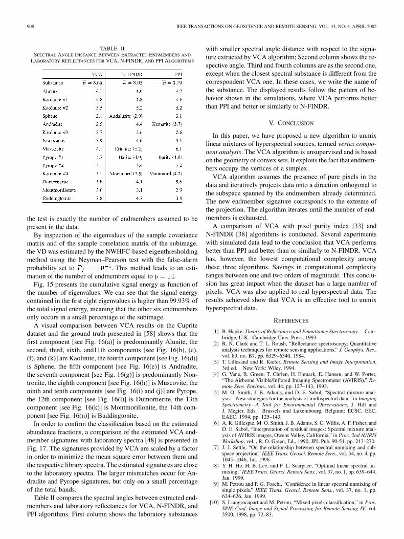
TABLE IISPECTRAL ANGLE DISTANCE BETWEEN EXTRACTED ENDMEMBERS AND

LABORATORY REFLECTANCES FOR VCA, N-FINDR, AND PPI ALGORITHMS

the test is exactly the number of endmembers assumed to bepresent in the data.

By inspection of the eigenvalues of the sample covariancematrix and of the sample correlation matrix of the subimage,the VD was estimated by the NWHFC-based eigenthresholdingmethod using the Neyman–Pearson test with the false-alarmprobability set to . This method leads to an esti-mation of the number of endmembers equal to .

Fig. 15 presents the cumulative signal energy as function ofthe number of eigenvalues. We can see that the signal energycontained in the first eight eigenvalues is higher than 99.93% ofthe total signal energy, meaning that the other six endmembersonly occurs in a small percentage of the subimage.

A visual comparison between VCA results on the Cupritedataset and the ground truth presented in [58] shows that thefirst component [see Fig. 16(a)] is predominantly Alunite, thesecond, third, sixth, and11th components [see Fig. 16(b), (c),(f), and (k)] are Kaolinite, the fourth component [see Fig. 16(d)]is Sphene, the fifth component [see Fig. 16(e)] is Andradite,the seventh component [see Fig. 16(g)] is predominantly Non-tronite, the eighth component [see Fig. 16(h)] is Muscovite, theninth and tenth components [see Fig. 16(i) and (j)] are Pyrope,the 12th component [see Fig. 16(l)] is Dumortierite, the 13thcomponent [see Fig. 16(k)] is Montmorillonite, the 14th com-ponent [see Fig. 16(n)] is Buddingtonite.

In order to confirm the classification based on the estimatedabundance fractions, a comparison of the estimated VCA end-member signatures with laboratory spectra [48] is presented inFig. 17. The signatures provided by VCA are scaled by a factorin order to minimize the mean square error between them andthe respective library spectra. The estimated signatures are closeto the laboratory spectra. The larger mismatches occur for An-dradite and Pyrope signatures, but only on a small percentageof the total bands.

Table II compares the spectral angles between extracted end-members and laboratory reflectances for VCA, N-FINDR, andPPI algorithms. First column shows the laboratory substances

with smaller spectral angle distance with respect to the signa-ture extracted by VCA algorithm; Second column shows the re-spective angle. Third and fourth columns are as the second one,except when the closest spectral substance is different from thecorrespondent VCA one. In these cases, we write the name ofthe substance. The displayed results follow the pattern of be-havior shown in the simulations, where VCA performs betterthan PPI and better or similarly to N-FINDR.

V. CONCLUSION

In this paper, we have proposed a new algorithm to unmixlinear mixtures of hyperspectral sources, termed vertex compo-nent analysis. The VCA algorithm is unsupervised and is basedon the geometry of convex sets. It exploits the fact that endmem-bers occupy the vertices of a simplex.

VCA algorithm assumes the presence of pure pixels in thedata and iteratively projects data onto a direction orthogonal tothe subspace spanned by the endmembers already determined.The new endmember signature corresponds to the extreme ofthe projection. The algorithm iterates until the number of end-members is exhausted.

A comparison of VCA with pixel purity index [33] andN-FINDR [38] algorithms is conducted. Several experimentswith simulated data lead to the conclusion that VCA performsbetter than PPI and better than or similarly to N-FINDR. VCAhas, however, the lowest computational complexity amongthese three algorithms. Savings in computational complexityranges between one and two orders of magnitude. This conclu-sion has great impact when the dataset has a large number ofpixels. VCA was also applied to real hyperspectral data. Theresults achieved show that VCA is an effective tool to unmixhyperspectral data.

REFERENCES

[1] B. Hapke, Theory of Reflectance and Emmittance Spectroscopy. Cam-bridge, U.K.: Cambridge Univ. Press, 1993.

[2] R. N. Clark and T. L. Roush, “Reflectance spectroscopy: Quantitativeanalysis techniques for remote sensing applications,” J. Geophys. Res.,vol. 89, no. B7, pp. 6329–6340, 1984.

[3] T. Lillesand and R. Kiefer, Remote Sensing and Image Interpretation,3rd ed. New York: Wiley, 1994.

[4] G. Vane, R. Green, T. Chrien, H. Enmark, E. Hansen, and W. Porter,“The Airborne Visible/Infrared Imaging Spectrometer (AVIRIS),” Re-mote Sens. Environ., vol. 44, pp. 127–143, 1993.

[5] M. O. Smith, J. B. Adams, and D. E. Sabol, “Spectral mixture anal-ysis—New strategies for the analysis of multispectral data,” in ImagingSpectrometry—A Tool for Environmental Observations, J. Hill andJ. Megier, Eds. Brussels and Luxembourg, Belgium: ECSC, EEC,EAEC, 1994, pp. 125–143.

[6] A. R. Gillespie, M. O. Smith, J. B. Adams, S. C. Willis, A. F. Fisher, andD. E. Sabol, “Interpretation of residual images: Spectral mixture anal-ysis of AVIRIS images, Owens Valley, California,” in Proc. 2nd AVIRISWorkshop, vol. , R. O. Green, Ed., 1990, JPL Pub. 90-54, pp. 243–270.

[7] J. J. Settle, “On the relationship between spectral unmixing and sub-space projection,” IEEE Trans. Geosci. Remote Sens., vol. 34, no. 4, pp.1045–1046, Jul. 1996.

[8] Y. H. Hu, H. B. Lee, and F. L. Scarpace, “Optimal linear spectral un-mixing,” IEEE Trans. Geosci. Remote Sens., vol. 37, no. 1, pp. 639–644,Jan. 1999.

[9] M. Petrou and P. G. Foschi, “Confidence in linear spectral unmixing ofsingle pixels,” IEEE Trans. Geosci. Remote Sens., vol. 37, no. 1, pp.624–626, Jan. 1999.

[10] S. Liangrocapart and M. Petrou, “Mixed pixels classification,” in Proc.SPIE Conf. Image and Signal Processing for Remote Sensing IV, vol.3500, 1998, pp. 72–83.


[11] N. Keshava and J. Mustard, “Spectral unmixing,” IEEE Signal Process.Mag., vol. 19, no. Jan., pp. 44–57, 2002.

[12] R. B. Singer and T. B. McCord, “Mars: Large scale mixing of brightand dark surface materials and implications for analysis of spectralreflectance,” in Proc. 10th Lunar and Planetary Sci. Conf., 1979, pp.1835–1848.

[13] B. Hapke, “Bidirection reflectance spectroscopy. I. Theory,” J. Geophys.Res., vol. 86, pp. 3039–3054, 1981.

[14] R. Singer, “Near-infrared spectral reflectance of mineral mixtures: Sys-tematic combinations of pyroxenes, olivine, and iron oxides,” J. Geo-phys. Res., vol. 86, pp. 7967–7982, 1981.

[15] B. Nash and J. Conel, “Spectral reflectance systematics for mixtures ofpowdered hypersthene, labradoride, and ilmenite,” J. Geophys. Res., vol.79, pp. 1615–1621, 1974.

[16] C. C. Borel and S. A. Gerstl, “Nonlinear spectral mixing models forvegetative and soils surface,” Remote Sens. Environ., vol. 47, no. 2, pp.403–416, 1994.

[17] C.-I Chang, Hyperspectral Imaging: Techniques for Spectral Detectionand Classification. New York: Kluwer, 2003.

[18] G. Shaw and H. Burke, “Spectral imaging for remote sensing,” LincolnLab. J., vol. 14, no. 1, pp. 3–28, 2003.

[19] D. Manolakis, C. Siracusa, and G. Shaw, “Hyperspectral subpixel targetdetection using linear mixing model,” IEEE Trans. Geosci. RemoteSens., vol. 39, no. 7, pp. 1392–1409, Jul. 2001.

[20] N. Keshava, J. Kerekes, D. Manolakis, and G. Shaw, “An algorithm tax-onomy for hyperspectral unmixing,” in Proc. SPIE AeroSense Conf. Al-gorithms for Multispectral and Hyperspectral Imagery VI, vol. 4049,2000, pp. 42–63.

[21] A. S. Mazer and M. Martin et al., “Image processing software forimaging spectrometry data analysis,” Remote Sens. Environ., vol. 24,no. 1, pp. 201–210, 1988.

[22] R. H. Yuhas, A. F. H. Goetz, and J. W. Boardman, “Discriminationamong semi-arid landscape endmembres using the Spectral AngleMapper (SAM) algorithm,” in Summaries 3rd Annu. JPL AirborneGeoscience Workshop, vol. 1, R. O. Green, Ed., 1992, JPL Publ. 92-14,pp. 147–149.

[23] J. C. Harsanyi and C.-I Chang, “Hyperspectral image classificationand dimensionality reduction: An orthogonal subspace projection ap-proach,” IEEE Trans. Geosci. Remote Sens., vol. 32, no. 4, pp. 779–785,Jul. 1994.

[24] C.-I Chang, X.-L. Zhao, M. L. G. Althouse, and J. J. Pan, “Least squaressubspace projection approach to mixed pixel classification for hyper-spectral images,” IEEE Trans. Geosci. Remote Sens., vol. 36, no. 3, pp.898–912, May 1998.

[25] D. C. Heinz, C.-I Chang, and M. L. G. Althouse, “Fully constrained leastsquares-based linear unmixing,” in Proc. IGARSS, 1999, pp. 1401–1403.

[26] P. Common, C. Jutten, and J. Herault, “Blind separation of sources, partII: Problem statement,” Signal Process., vol. 24, pp. 11–20, 1991.

[27] J. Bayliss, J. A. Gualtieri, and R. Cromp, “Analysing hyperspectraldata with independent component analysis,” Proc. SPIE, vol. 3240, pp.133–143, 1997.

[28] C. Chen and X. Zhang, “Independent component analysis for remotesensing study,” in Proc. SPIE Symp. Remote Sensing Conf. Image andSignal Processing for Remote Sensing V, vol. 3871, 1999, pp. 150–158.

[29] T. M. Tu, “Unsupervised signature extraction and separation in hyper-spectral images: A noise-adjusted fast independent component analysisapproach,” Opt. Eng., vol. 39, no. 4, pp. 897–906, 2000.

[30] S.-S. Chiang, C.-I Chang, and I. W. Ginsberg, “Unsupervised hyper-spectral image analysis using independent component analysis,” in Proc.IGARSS, vol. 7, 2000, pp. 3136–3138.

[31] J. M. P. Nascimento and J. M. B. Dias, “Does independent componentanalysis play a role in unmixing hyperspectral data?,” in Pattern Recog-nition and Image Analysis. ser. , F. J. Perales, A. Campilho, and N. P. B.A. Sanfeliu, Eds. Berlin, Germany: Springer-Verlag, 2003, vol. 2652,Lecture Notes in Computer Science, pp. 616–625.

[32] A. Ifarraguerri and C.-I Chang, “Multispectral and hyperspectral imageanalysis with convex cones,” IEEE Trans. Geosci. Remote Sens., vol. 37,no. 2, pp. 756–770, Mar. 1999.

[33] J. Boardman, “Automating spectral unmixing of AVIRIS data usingconvex geometry concepts,” in Summaries 4th Annu. JPL AirborneGeoscience Workshop, vol. 1, 1993, JPL Pub. 93-26, pp. 11–14.

[34] M. D. Craig, “Minimum-volume transforms for remotely sensed data,”IEEE Trans. Geosci. Remote Sens., vol. 32, no. 1, pp. 99–109, Jan. 1994.

[35] C. Bateson, G. Asner, and C. Wessman, “Endmember bundles: Anew approach to incorporating endmember variability into spectralmixture analysis,” IEEE Trans. Geosci. Remote Sens., vol. 38, no. 2, pp.1083–1094, Mar. 2000.

[36] R. Seidel, Convex Hull Computations. Boca Raton, FL: CRC, 1997,ch. 19, pp. 361–375.

[37] S. Geman and D. Geman, “Stochastic relaxation, Gibbs distribution andthe Bayesian restoration of images,” IEEE Trans. Pattern Anal. Mach.Intell., vol. 6, no. 6, pp. 721–741, Jun. 1984.

[38] M. E. Winter, “N-findr: An algorithm for fast autonomous spectralend-member determination in hyperspectral data,” in Proc. SPIE Conf.Imaging Spectrometry V, 1999, pp. 266–275.

[39] J. Boardman, F. A. Kruse, and R. O. Green, “Mapping target signaturesvia partial unmixing of AVIRIS data,” in Summaries 5th JPL AirborneEarth Science Workshop, vol. 1, 1995, pp. 23–26.

[40] J. Theiler, D. Lavenier, N. Harvey, S. Perkins, and J. Szymanski, “Usingblocks of skewers for faster computation of pixel purity index,” pre-sented at the SPIE Int. Conf. Optical Science and Technology, 2000.

[41] D. Lavenier, J. Theiler, J. Szymanski, M. Gokhale, and J. Frigo, “FPGAimplementation of the pixel purity index algorithm,” presented at theProc. SPIE Photonics East, Workshop on Reconfigurable Architectures,2000.

[42] J. H. Bowles, P. J. Palmadesso, J. A. Antoniades, M. M. Baumback, andL. J. Rickard, “Use of filter vectors in hyperspectral data analysis,” inProc. SPIE Conf. Infrared Spaceborne Remote Sensing III, vol. 2553,1995, pp. 148–157.

[43] J. H. Bowles, J. A. Antoniades, M. M. Baumback, J. M. Grossmann,D. Haas, P. J. Palmadesso, and J. Stracka, “Real-time analysis of hyper-spectral data sets using NFL’s orasis algorithm,” in Proc. SPIE Conf.Imaging Spectrometry III, vol. 3118, 1997, pp. 38–45.

[44] J. M. Grossmann, J. Bowles, D. Haas, J. A. Antoniades, M. R. Grunes,P. Palmadesso, D. Gillis, K. Y. Tsang, M. Baumback, M. Daniel, J.Fisher, and I. Triandaf, “Hyperspectral analysis and target detectionsystem for the Adaptative Spectral Reconnaissance Program (ASRP),”in Proc. SPIE Conf. Algorithms for Multispectral and HyperspectralImagery IV, vol. 3372, 1998, pp. 2–13.

[45] I. T. Jolliffe, Principal Component Analysis. New York: Springer-Verlag, 1986.

[46] A. Green, M. Berman, P. Switzer, and M. D. Craig, “A transformation forordering multispectral data in terms of image quality with implicationsfor noise removal,” IEEE Trans. Geosci. Remote Sens., vol. 26, no. 1,pp. 65–74, Jan. 1994.

[47] L. L. Scharf, Statistical Signal Processing, Detection Estimation andTime Series Analysis. Reading, MA: Addison-Wesley, 1991.

[48] R. N. Clark, G. A. Swayze, A. Gallagher, T. V. King, and W. M. Calvin,“The U.S. Geological Survey digital spectral library: Version 1: 0.2 to3.0 �m,” U.S. Geol. Surv., Denver, CO, Open File Rep. 93-592, 1993.

[49] J. H. Bowles, M. Daniel, J. M. Grossmann, J. A. Antoniades, M. M.Baumback, and P. J. Palmadesso, “Comparison of output from orasis andpixel purity calculations,” in Proc. SPIE Conf. Imaging Spectrometry IV,vol. 3438, 1998, pp. 148–156.

[50] A. Plaza, P. Martinez, R. Perez, and J. Plaza, “Spatial/spectral end-member extraction by multidimensional morphological operations,”IEEE Trans. Geosci. Remote Sens., vol. 40, no. 9, pp. 2025–2041, Sep.2002.

[51] , “A quantitative and comparative analysis of endmember extrac-tion algorithms from hyperspectral data,” IEEE Trans. Geosci. RemoteSens., vol. 42, no. 3, pp. 650–663, Mar. 2004.

[52] S. Kullback, Information Theory and Statistics, Peter Smith, London,U.K., 1978.

[53] C. Chang, “An information-theoretic approach to spectral variability,similarity, and discrimination for hyperspectral image analysis,” IEEETrans. Inf. Theory, vol. 46, no. 5, pp. 1927–1932, Aug. 2000.

[54] E. Kaltofen and G. Villard, “On the complexity of computing determi-nants,” in Proc. 5th Asian Symp. Computer Mathematics, vol. 9, LectureNotes Series on Computing, K. Shirayanagi and K. Yokoyama, Eds.,Singapore, 2001, pp. 13–27.

[55] G. Swayze, R. Clark, S. Sutley, and A. Gallagher, “Ground-truthingaviris mineral mapping at Cuprite, Nevada,” in Summaries 3rd Annu.JPL Airborne Geosciences Workshop, vol. 1, 1992, pp. 47–49.

[56] R. Ashley and M. Abrams, “Alteration mapping uing multispectral im-ages—Cuprite Mining District, Esmeralda County,” U.S. Geol. Surv.,Denver, CO, Open File Rep. 80-367, 1980.

[57] M. Abrams, R. Ashley, L. Rowan, A. Goetz, and A. Kahle, “Mappingof hydrothermal alteration in the Cuprite Mining District, Nevada, usingaircraft scanner images for the spectral region 0.46 to 2.36 mm,” Ge-ology, vol. 5, pp. 713–718, 1977.

[58] G. Swayze, “The hydrothermal and structural history of the CupriteMining District, southwestern Nevada: An integrated geological andgeophysical approach,” Ph.D. dissertation, Univ. Colorado, Boulder,1997.


[59] A. Goetz and V. Strivastava, “Mineralogical mapping in the cupritemining district,” in Proc. Airborne Imaging Spectrometer Data AnalysisWorkshop, 1985, JPL Pub. 5-41, pp. 22–29.

[60] F. Kruse, J. Boardman, and J. Huntington, “Comparision of EO-1 Hy-perion and airborne hyperspectral remote sensing data for geologic ap-plications,” presented at the SPIE Aerospace Conf., 2002.

[61] C.-I Chang and Q. Du, “Estimation of number of spectrally distinctsignal sources in hyperspectral imagery,” IEEE Trans. Geosci. RemoteSens., vol. 42, no. 3, pp. 608–619, Mar. 2004.

[62] J. Harsanyi, W. Farrand, and C.-I Chang, “Determining the numberand identity of spectral endmembers: An integrated approach usingNeyman–Pearson eigenthresholding and iterative constrained rms errorminimization,” presented at the 9th Thematic Conf. Geologic RemoteSensing, 1993.

José M. P. Nascimento (S’03) received the B. S. andE.E. degree from Instituto Superior de Engenharia deLisboa, Politechnic Institute of Lisbon, Lisbon, Por-tugal, and the M.Sc. degree in electrical and com-puter engineer from Instituto Superior Técnico (IST),Technical University of Lisbon, in 1993, 1995, and2000, respectively. He is currently pursuing the Ph.D.degree in electrical engineering at Instituto SuperiorTécnico, Technical University of Lisbon.

He is currently a Professor in the Department ofElectronics, Telecommunications and Computer’s

Engineering, Instituto Superior de Engenharia de Lisboa. He is also Researcherwith the Institute of Telecommunications. His research interests include remotesensing, signal and image processing, pattern recognition, and communications.

José M. Bioucas Dias (S’87–M’95) received theE.E., M.Sc., and Ph.D. degrees in electrical andcomputer engineering from the the Instituto SuperiorTécnico (IST), Technical University of Lisbon,Lisbon, Portugal, in 1985, 1991, and 1995, respec-tively.

He is currently an Assistant Professor with theDepartment of Electrical and Computer Engineering,IST. He is also a Researcher with the CommunicationTheory and Pattern Recognition Group, IST. Hisresearch interests include remote sensing, signal and

image processing, pattern recognition, and communications.

Documents

898 IEEE TRANSACTIONS ON GEOSCIENCE AND REMOTE …bioucas/files/ieeegrsVca04.pdf · 898 IEEE TRANSACTIONS ON GEOSCIENCE AND REMOTE SENSING, VOL. 43, NO. 4, APRIL 2005 Vertex Component