8.3.1.1 Models Used and Their Linkages - California

Water Quality

Bay Delta Conservation Plan/California WaterFix Final EIR/EIS

Administrative Final 8-140

2016 ICF 00139.14

locations, then that Alternative was determined to have an adverse water quality effect (under 1 NEPA) and a significant impact on water quality (under CEQA) for that water quality constituent or 2 parameter. Improvements to water quality conditions, where modeled or estimated to occur, also 3 were generally identified as beneficial if considered to reflect a substantial change. 4

In summary, the impact assessment methodology includes the following: 5

1. Addresses all constituents of concern based on available information and the current science 6 regarding concentrations/levels that would affect beneficial uses of waters within the affected 7 environment. 8

2. Quantitatively evaluates constituents of primary concern where modeling tools were developed 9 and were available for doing so, and qualitatively assesses effects where appropriate modeling 10 tools were unavailable. 11

3. Evaluates the overall effect of the alternatives on beneficial uses in a comparative manner 12 throughout the affected environment, during three distinct time frames, which address climate 13 change considerations. 14

The details of this methodological approach are discussed below. In the following sections, the 15 specific methodologies used to assess water quality impacts within the three distinct areas of the 16 affected environment (i.e., Upstream of the Delta, Plan Area, and SWP/CVP Export Service Areas) are 17 discussed. 18

8.3.1.1 Models Used and Their Linkages 19

The models used in support of the quantitative water quality analyses were: (1) Reclamation and 20 DWR’s CALSIM II hydrologic model; and (2) DWR’s DSM2. A description of each model is provided 21 below, including a discussion of how the models were used to assess compliance with water quality 22 objectives for EC and chloride in the Delta, as well as how results from these models were used to 23 quantify changes in other water quality constituent concentrations/parameter levels. More 24 information on these models and the assumptions included in their application is described in 25 Appendix 5A, BDCP/California WaterFix FEIR/FEIS Modeling Technical Appendix. 26

CALSIM II 27

The CALSIM II model, which has been jointly developed and maintained by DWR and Reclamation to 28 provide hydrologic-based information for planning, managing, and operating the integrated SWP 29 and CVP system, was used to simulate system operations and resulting hydrologic conditions under 30 the alternatives. CALSIM II operates on a monthly time step from water year 1922 through 2003 31 using historical rainfall and runoff data which have been adjusted for changes in water and land uses 32 that have occurred or are projected to occur in the future. In the model, the reservoirs and pumping 33 facilities of the SWP and CVP are operated to ensure the flow and water quality requirements for 34 these systems are met. The model assumes that facilities, land uses, water supply contracts, and 35 regulatory requirements are constant throughout the 82-year hydrologic period of record, thus 36 providing a simulation representing a fixed level of development. Among other output, CALSIM II 37 provides end-of-month reservoir storage levels, and mean monthly reservoir releases, flows at 38 various locations along the major rivers, X2 location, Delta inflow, and Delta outflow for the 82-year 39 hydrologic period of record. 40

CCC-SC-25

Water Quality



2016 ICF 00139.14

The 2010 version of CALSIM II was used to model the SWP and CVP system and, thus, support the 1 assessments in this chapter. This differs from the version being used to support the Biological 2 Assessment being prepared for the proposed project, which is the 2015 version of CALSIM II. For the 3 reasons described in Appendix 5F, the modeling results presented herein may differ from those 4 presented in the Biological Assessment; however, the nature of those differences would not lead to 5 different impact conclusions from those presented herein. Input assumption details for each 6 scenario modeled using CALSIM II are provided in Appendix 5A, BDCP/California WaterFix 7 FEIR/FEIS Modeling Technical Appendix. 8

The primary linkage of these models is for CALSIM II output to serve as input to DSM2, as shown in 9 Figure 8-50. Key considerations in the CALSIM II modeling logic for the water quality assessment 10 include how CALSIM II operations rules are configured to meet particular Delta water quality 11 objectives for salinity and how daily patterning techniques were applied to the monthly CALSIM II 12 operations. These topics are addressed further below. 13

Artificial Neural Network for Flow-Salinity Relationship 14

Flow-salinity relationships in the Delta are critical to both SWP/CVP and ecosystem management. 15 Operation of the SWP/CVP facilities and management of Delta exports are often dependent on Delta 16 flow needs for meeting salinity standards. Salinity in the Delta cannot be simulated accurately by the 17 simple mass-balance routing and coarse time-step used in CALSIM II. An Artificial Neural Network 18 (ANN) has been developed (Sandhu et al. 1999) that attempts to mimic the flow-salinity 19 relationships as simulated in DSM2, but provides a rapid transformation of this information into a 20 form usable by the CALSIM II operations model. The ANN is implemented in CALSIM II to constrain 21 the operations of the upstream reservoirs and the Delta export pumps in order to satisfy particular 22 salinity requirements. A more detailed description of the use of ANNs in the CALSIM II model is 23 provided in Wilbur and Munévar (2001: Chapter 7). 24

The flow-salinity ANN developed by DWR (Sandhu et al. 1999, Seneviratne and Wu 2007) attempts 25 to statistically correlate the salinity results from a particular DSM2 run to the various peripheral 26 flows (Delta inflows, exports and diversions), gate operations, and an indicator of tidal energy. The 27 ANN is calibrated, or trained, on DSM2 results that represent a specific Delta configuration using a 28 full circle analysis (Seneviratne and Wu 2007). For example, a future reconfiguration of the Delta 29 channels to improve conveyance may significantly affect the hydrodynamics of the system. The ANN 30 would be able to represent this new configuration by being retrained by DSM2 results that included 31 the new configuration. The ANN approximates DSM2-generated salinity at the following key 32 locations for the purpose of modeling Delta water quality standards: Sacramento River at Emmaton, 33 San Joaquin River at Jersey Point, Sacramento River at Collinsville, and Old River at Rock Slough. In 34 addition, the ANN is capable of providing salinity estimates for Clifton Court Forebay, CCWD 35 Alternate Intake Project (AIP) and Los Vaqueros diversion locations. The ANN may not fully capture 36 the dynamics of the Delta under conditions other than those for which it was trained. It is possible 37 that the ANN will exhibit errors in flow regimes beyond those for which it was trained. Therefore, a 38 new ANN was developed for scenarios with sea level rise and/or restoration areas in the Delta 39 which result in changed flow–salinity relationships in the Delta. A more complete description of the 40 ANNs developed and used is included in Appendix 5A, Section A.5.3. 41

Monthly-to-Daily Patterning for Sacramento River at Freeport 42

In an effort to better represent the sub-monthly flow variability, particularly in early winter, a 43 monthly-to-daily flow patterning technique is applied directly in CALSIM II for the Fremont Weir, 44

CCC-SC-25

Water Quality



2016 ICF 00139.14

Sacramento Weir, and the north Delta intakes. The technique applies historical daily patterns, based 1 on the hydrology of the year, to transform the monthly volumes into daily flows. In all cases, the 2 monthly volumes are preserved between the daily and monthly flows. It is important to note that 3 this daily patterning approach does not in any way represent the flows resulting from operational 4 responses on a daily time step. It is simply a technique to incorporate representative daily 5 variability into the flows resulting from CALSIM II’s monthly operational decisions to help provide a 6 better estimate of the Fremont and Sacramento weir spills, which are sensitive to the daily flow 7 patterns and provides the upper bound of the available north Delta diversion in the alternatives. The 8 incorporation of daily patterning in CALSIM II is described in the Section A.3.3 of Appendix 5A, 9 BDCP/California WaterFix FEIR/FEIS Modeling Technical Appendix. 10

DSM2 11

DSM2 is a one-dimensional mathematical model for dynamic simulation of hydrodynamics, water 12 quality, and particle tracking throughout the Delta. DSM2 can be used to calculate stages, flows, 13 velocities, mass transport processes for conservative constituents, and transport of individual 14 particles. The model runs on a 15-minute time step for a 16-year hydrologic period of record. DSM2 15 currently consists of three modules: HYDRO, QUAL, and PTM. HYDRO simulates one-dimensional 16 hydrodynamics including flows, velocities, depth, and water surface elevations. HYDRO provides the 17 flow input for QUAL and PTM. QUAL simulates one-dimensional fate and transport of conservative 18 water quality constituents given a flow field simulated by HYDRO. PTM simulates pseudo three-19 dimensional transport of neutrally buoyant particles based on the flow field simulated by HYDRO. 20 Input assumption details for each scenario modeled are provided in Appendix 5A. 21

Simulation Period 22

DSM2 was utilized to simulate the 16-year, 1976–1991 hydrologic period of record. This hydrologic 23 period of record contains a sequence of water years that contains all water year types: wet, above 24 normal, below normal, dry, and critical. This hydrologic period is bracketed at each end by two 25 critical years: 1976 and 1977 at the beginning of the period and 1990 and 1991 at the end of the 26 period. This hydrologic period also contains an extended drought period, 1987–1991. Additional 27 information regarding the selection of the simulation period is provided in Appendix 5A, Section D 28 (Additional Modeling Information). 29

Monthly-to-Daily Patterning 30

DSM2 is simulated on a 15-minute time step to address the changing tidal dynamics of the Delta 31 system. However, the boundary flows, which are provided from CALSIM II output, are mean monthly 32 flows. As shown in Figures A-6 and A-7 of Appendix 5A, Sacramento River flow at Freeport exhibits 33 significant daily variability around the monthly mean in the winter and spring periods in most water 34 year types. The winter-spring daily flow variability is deemed important to aquatic species of 35 concern. To better represent the sub-monthly flow variability, particularly in early winter, a 36 monthly-to-daily flow patterning technique was applied to the boundary flow inputs to DSM2. The 37 monthly-to-daily flow patterning approach used in CALSIM II and DSM2 are consistent. A detailed 38 description of the implementation of the daily variability in DSM2 boundary flows is provided in 39 Appendix 5A, Section D.9. 40

It is important to note that this monthly-to-daily patterning approach does not in any way represent 41 the flows that would result from any operational responses on a daily time step. It is simply a 42

CCC-SC-25

Water Quality



2016 ICF 00139.14

technique to incorporate representative daily variability into the flows resulting from CALSIM II’s 1 monthly operational decisions. 2

Calibration and Validation 3

DSM2 hydrodynamics and salinity (EC), which is directly modeled by DSM2, were initially calibrated 4 in 1997 (California Department of Water Resources 1997). In 2000, a group of agencies, water users, 5 and stakeholders recalibrated and validated DSM2 in an open process resulting in a model that 6 could replicate the observed data more closely than the 1997 version (DSM2PWT 2001). In 2009, 7 CH2M HILL performed a calibration and validation of DSM2 by including the flooded Liberty Island 8 in the DSM2 grid, which allowed for an improved simulation of tidal hydraulics and EC transport in 9 DSM2 (CH2M HILL 2009). The technical report documenting this calibration and validation effort is 10 included in Appendix 5A, Section D.5. Simulation of DOC transport in DSM2 was successfully 11 validated in 2001 by DWR (Pandey 2001). The version of DSM2 used for evaluating the alternatives 12 incorporates these latest calibrations. 13

Corroboration 14

To evaluate DSM2’s ability to represent the effects of sea level change and the proposed restoration 15 actions on Delta hydrodynamics and salinity, DSM2 results were compared with results from two 16 other Delta simulation models. The effects of sea level rise were simulated by the three-dimensional 17 UNTRIM Bay-Delta model and the effects of tidal marsh restoration were simulated by the two-18 dimensional RMA Bay-Delta model. Detailed descriptions of the UnTRIM modeling of the sea level 19 rise scenarios, RMA modeling of the tidal marsh restoration, and DSM2 corroboration are included 20 in Appendix 5A, Sections D.7, D.6, and D.8, respectively. Overall the results show that DSM2 is 21 capable of simulating similar incremental changes in flows and salinity at most Delta locations as in 22 the RMA model. Further, DSM2 is capable of simulating similar incremental changes in salinity as 23 UnTRIM in the west Delta where sea level rise is expected to have an influence. 24

Modeling Limitations and Uncertainty 25

Because DSM2 is a one-dimensional model, it has inherent limitations in simulating hydrodynamic 26 and transport processes in a complex estuarine environment such as the Delta. DSM2 assumes that 27 velocity in a channel can be adequately represented by a single average velocity over the channel 28 cross-section, meaning that variations both across the width of the channel and through the water 29 column are negligible. DSM2 does not have the ability to model short-circuiting of flow through a 30 reach, where a majority of the flow in a cross-section is confined to a small portion of the cross-31 section. DSM2 does not conserve momentum at the channel junctions and does not model the 32 secondary currents in a channel. DSM2 also does not explicitly account for dispersion due to flow 33 accelerating through channel bends. It cannot model the vertical salinity stratification in the 34 channels. It has inherent limitations in simulating the hydrodynamics related to the open water 35 areas. Since a reservoir surface area is constant in DSM2, it impacts the stage in the reservoir and 36 thereby impacting the flow exchange with the adjoining channel. Due to the inability to change the 37 cross-sectional area of the reservoir inlets with changing water surface elevation, the final entrance 38 and exit coefficients were fine tuned to match a median flow range. This causes errors in the flow 39 exchange at breaches during the extreme spring and neap tides. Using an arbitrary bottom elevation 40 value for the reservoirs representing the proposed marsh areas to get around the wetting-drying 41 limitation of DSM2 may increase the dilution of salinity in the reservoirs. Accurate representation of 42

CCC-SC-25

Water Quality



2016 ICF 00139.14

tidal marsh areas, bottom elevations, location of breaches, breach widths, cross-sections, and 1 boundary conditions in DSM2 is critical to the corroboration with RMA results for tidal marsh areas. 2

For open water bodies DSM2 assumes uniform and instantaneous mixing over an entire open water 3 area. Thus it does not account for the salinity gradients that may exist within the open water bodies. 4 Significant uncertainty exists in flow and EC input data related to in-Delta agriculture, which leads to 5 uncertainty in the simulated EC values. Caution needs to be exercised when using EC outputs on a 6 sub-monthly scale. Water quality results inside the water bodies representing the tidal marsh areas 7 were not validated specifically. Additionally, localized withdrawals and returns are not simulated for 8 Suisun Marsh in DSM2. In some areas of Suisun Marsh where these play a major role in water 9 quality, DSM2 modeling may not be accurate. 10

Notwithstanding the above limitation, DSM2 remains the best available tool from which to simulate 11 water quality changes within the Delta over an extended hydrologic period. 12

Use of CALSIM II and DSM2 for Assessment of Meeting of Bay-Delta WQCP Water 13 Quality Objectives 14

Water Quality Objectives Incorporated into CALSIM II 15

In CALSIM II, the reservoirs and facilities of the SWP and CVP are operated to assure the flow and 16 water quality requirements for these systems are met. Meeting regulatory requirements, including 17 Delta water quality objectives, is the highest operational priority in CALSIM II. As mentioned above, 18 CALSIM II uses an ANN to configure system operations to meet salinity objectives. Because CALSIM 19 II operates on a monthly time step, the model attempts to meet these objectives on a monthly 20 average basis, even though the objectives themselves are often based on 14-day or 30-day running 21 averages, and may start or end in the middle of a month. The ANN can only predict salinity at a few 22 of the locations that have water quality objectives for salinity, which are specific to Delta beneficial 23 uses: 24

Municipal and Industrial Use: 25

Old River at Rock Slough 26

Banks/Jones Pumping Plants 27

Agricultural Beneficial Use: 28

Sacramento River at Emmaton or Threemile Slough 29

San Joaquin River at Jersey Point 30

Fish and Wildlife Beneficial Uses: 31

Sacramento River at Collinsville 32

At the locations denoted above, because meeting the objectives is the highest priority in CALSIM II, 33 only two conditions in CALSIM II are possible: (1) applicable water quality objectives are met on a 34 monthly average basis according to the ANN, or (2) there is no feasible way to meet the objective. 35

Note that the certain alternatives contain an important element regarding the Sacramento River at 36 Emmaton water quality objective. Alternatives 1A–C, 2A–C, 3, 5, 6A–C, 7, 8, and 9 include, as part of 37 the definition of the alternative, a change in the compliance point to the Sacramento River at 38 Threemile Slough. The ANN for these alternatives was retrained based on this change, so CALSIM II 39

CCC-SC-25

Water Quality



2016 ICF 00139.14

operated in such a way as to meet this objective at Threemile Slough under these alternatives. The 1 Existing Conditions and No Action Alternative did not include this change to the compliance point or 2 ANN. Also, for Alternatives 4, 4A, 2D, and 5C, the Sacramento River at Emmaton compliance location 3 is retained. 4

Threemile Slough is located approximately two and one-half miles upstream of Emmaton. Because 5 of their relative locations, when the EC water quality objective is met at Emmaton, it is generally also 6 met at Threemile Slough. However, it is not always the case that meeting the objective at Threemile 7 Slough results in meeting the objective at Emmaton, because the Threemile Slough is further 8 upstream from the effects that salinity intrusion can have on EC. Thus, under the alternatives that 9 include a change in compliance location from Emmaton to Threemile Slough, there are more 10 exceedances of the water quality objective at Emmaton (were it to be still in place) than under the 11 Existing Conditions or No Action Alternative (which do have the compliance location at Emmaton). 12

When DSM2 is run using the output from CALSIM II, exceedances of the water quality objectives 13 above can occur for the reasons below. 14

1. CALSIM II found no feasible way to meet the objective – i.e., both CALSIM II and DSM2 agree that 15 the objective is exceeded. 16

2. The ANN that CALSIM II uses predicted that the objective would be met on a monthly average 17 basis under the operations simulated in CALSIM II, but either: 18

a. The ANN is an imperfect predictor of compliance generally, or specifically on the time-step 19 and averaging basis by which these objectives are defined; or 20

b. The monthly-to-daily patterning discussed above resulted in a pattern of flows at the DSM2 21 boundary conditions that resulted in the objective being exceeded. 22

In the water quality analysis, if exceedances of these objectives were predicted via the DSM2 results, 23 depending on the specific objective in question, various approaches were employed to determine if 24 the exceedances fell into reason 1 or 2 above. If they fell into reason 2 (i.e., objective met in CALSIM 25 II), additional sensitivity analyses were performed to determine if changes in modeling assumptions 26 or operational changes could result in compliance with the objective. Additional information 27 regarding these analyses is provided in Appendix 8H, Electrical Conductivity, Attachments 1 and 2. 28

Water Quality Objectives not Incorporated into CALSIM II 29

There are also water quality objectives for salinity that are not incorporated into the ANN and 30 CALSIM II. These include objectives that apply for the following beneficial uses and locations: 31

Municipal and Industrial Use: 32

Cache Slough at City of Vallejo Intake 33

Barker Slough at North Bay Aqueduct Intake 34

Agricultural Beneficial Use: 35

Interior Delta 36

South Fork Mokelumne River at Terminous 37

San Joaquin River at San Andreas Landing 38

Southern Delta and Export Area 39

CCC-SC-25

Water Quality



2016 ICF 00139.14

San Joaquin River at Airport Way Bridge, Vernalis 1

San Joaquin River at Brandt Bridge Site 2

Old River near Middle River 3

Old River at Tracy Road Bridge 4

West Canal at mouth of Clifton Court Forebay 5

Delta-Mendota Canal at Tracy Pumping Plant 6

Fish and Wildlife Beneficial Uses: 7

San Joaquin River at and between Jersey Point and Prisoners Point 8

Suisun Marsh 9

Sacramento River at Collinsville 10

Montezuma Slough at National Steel 11

Montezuma Slough near Beldon’s Landing 12

Chadbourne Slough at Sunrise Duck Club 13

Suisun Slough, 300 feet south of Volanti Slough 14

Cordelia Slough at lbis Club 15

Goodyear Slough at Morrow Island Clubhouse 16

Water supply intakes for waterfowl management areas on Van Sickle and Chipps Islands 17

Although CALSIM II does not specifically operate to meet these objectives, they are nonetheless 18 often if not always incidentally met when DSM2 is run using the CALSIM II output as boundary 19 conditions. Meeting of some of these objectives is not directly related to operations that CALSIM II 20 simulates. For example, some of these objectives relate more to discharges and local sources of 21 salinity, as opposed to system-wide operation. Others, specifically the fish and wildlife objectives in 22 Suisun Marsh, are based on sub-daily (i.e., high tide) EC values, and also take into account other 23 factors related to effects on wildlife when evaluating exceedance of an objective, and thus CALSIM II 24 cannot operate to specifically meet the objective. When DSM2 is run using the output from CALSIM 25 II, exceedances of the water quality objectives above can occur for the following reasons. 26

1. The exceedances are real reflections of water quality conditions for the given scenario due to 27 system operations simulated in the CALSIM II model run and other assumptions inherent in the 28 DSM2 run. 29

2. The system operations that CALSIM II simulated were incidentally sufficient to meet the water 30 quality objective on a monthly average basis, but the monthly-to-daily patterning discussed 31 above resulted in a pattern of flows at the DSM2 boundary conditions that resulted in the 32 objective being exceeded. 33

In the water quality analysis, if exceedances of these objectives were predicted via the DSM2 results, 34 depending on the specific objective in question, various approaches were employed to determine if 35 the exceedances fell into reason 1 or 2 above. If they fell into reason 1 (i.e., exceedances are due to 36 system operations), additional sensitivity analyses were performed to determine if changes in 37 modeling assumptions or operational changes could result in compliance with the objective. 38

CCC-SC-25

Water Quality



2016 ICF 00139.14

Additional information regarding these analyses is provided in Appendix 8H, Electrical Conductivity, 1 Attachments 1 and 2. 2

Real-Time Operations of the SWP and CVP 3

In reality, staff from DWR and Reclamation constantly monitor Delta water quality conditions and 4 adjust operations of the SWP and CVP in real time as necessary to meet water quality objectives. 5 These decisions take into account real-time conditions and are able to account for many factors that 6 the best available models cannot simulate. In Section 8.1.3.4 and 8.1.3.7, the history of compliance 7 with Delta water quality objectives is summarized and discussed. In the 30-plus year history of the 8 water quality standards, there are relatively few instances in which water quality objectives were 9 exceeded when SWP and CVP operations had any ability to prevent the exceedance (see Sections 10 8.1.3.4 and 8.1.3.7 for more detail). Environmental conditions arise that cannot be foreseen or 11 simulated in the model that can affect compliance with water quality objectives. These include 12 unpredictable tidal and/or wind conditions, gate failures, operational needs to improve fish 13 habitat/conditions, and prolonged extreme drought conditions, among others. At times, negotiations 14 with the State Water Resources Control Board occur in order to effectively maximize and balance 15 protection of beneficial uses and water rights. These activities are expected to continue in the future. 16 Thus, it is likely that some objective exceedances simulated in the modeling would not occur under 17 the real-time monitoring and operational paradigm that will be in place to prevent such 18 exceedances. 19

8.3.1.2 Upstream of the Delta Region 20

Water quality changes in the affected environment upstream from the north-Delta boundary, which 21 includes the Sacramento River to Shasta Lake, the Feather River to Lake Oroville, and the American 22 River to Folsom Lake, were primarily assessed qualitatively. Assessment of water quality changes 23 was limited to facilities operations-related water quality changes for all alternatives, and the 24 implementation of CM2–CM21 for the BDCP alternatives or Environmental Commitments under 25 Alternatives 4A, 2D, and 5A. Conveyance facility construction-related effects are not anticipated 26 upstream of the Delta. 27

The assessment of water quality changes in water bodies upstream of the Delta relied, in part, on 28 making determinations as to how reservoir storage and releases would be changed. Specific changes 29 in reservoir storage and releases were determined from CALSIM II modeling of the SWP and CVP 30 system (Appendix 5A, BDCP/California WaterFix FEIR/FEIS Modeling Technical Appendix, describes 31 the CALSIM II modeling performed in support of this assessment). Reservoir storage and river flow 32 changes were then evaluated to make determinations regarding the capacity for the affected water 33 bodies to provide dilution of watershed contaminant inputs. Also, if a particular parameter was 34 found to be correlated to seasonal reservoir levels or river flows, how the parameter would be 35 altered seasonally by operational changes in reservoir levels or river flows was assessed. 36

8.3.1.3 Plan Area 37

Water quality changes in the Delta were assessed quantitatively to the extent that data and models 38 were available to do so; otherwise, water quality changes were assessed qualitatively. Using the 39 methodology described below, changes in boron, bromide, chloride, mercury, methylmercury, 40 nitrate, organic carbon, and selenium within the Delta were determined quantitatively at 41

CCC-SC-25

Water Quality



2016 ICF 00139.14

11 assessment locations (Figure 8-7), while electrical conductivity and chloride were assessed at D-1 1641 compliance locations. 2

Operations-related water quality changes (i.e., CM1 under the BDCP alternatives) would be partly 3 driven by geographic and hydrodynamic changes resulting from restoration actions (i.e., altered 4 hydrodynamics attributable to new areas of tidal wetlands (CM4), for example). There is no way to 5 disentangle the hydrodynamic effects of CM4 and other restoration measures from CM1, since the 6 Delta as a whole is modeled with both CM1 and the other conservation measures implemented. To 7 the extent that restoration actions alter hydrodynamics within the Delta region, which affects mixing 8 of source waters, these effects were included in the modeling assessment of operations-related 9 water quality changes (CM1 under the BDCP alternatives). Other effects of CM2–CM21 not 10 attributable to hydrodynamics, for example, additional loading of a water quality constituent to the 11 Delta, are discussed within the impact heading for CM2–CM21. 12

Methodologies to determine the effects attributable to construction activities and actions to address 13 the other stressors are discussed later in this section. 14

Constituent Screening Analysis 15

Constituents assessed in the water quality chapter were identified based on the following 16 considerations. 17

Availability of historical monitoring data. 18

Constituents having adopted federal water quality criteria or state water quality objectives. 19

Constituents on the state’s CWA Section 303(d) list in the Delta. 20

Constituents identified in public scoping comments. 21

Constituents deserving assessment based on professional judgment. 22

A constituent screening analysis was conducted on 182 water quality constituents/parameters. The 23 screening analysis determined which constituents had no potential to exceed the thresholds of 24 significance by implementation of the alternatives and, thus, did not warrant further assessment. 25 This analysis identified a list of “constituents of concern” that were further analyzed as part of 26 assessing their potential water quality related impacts under the alternatives. For a detailed 27 description of the approach employed in the constituent screening analysis, see Appendix 8C, 28 Screening Analysis. 29

Determining Whether Assessment is Qualitative or Quantitative 30

For many constituents, lack of adequate representative data precluded a quantitative assessment. 31 Tables SA-8 and SA-9 of Appendix 8C identify the types of constituents that were carried forward for 32 detailed analysis and were automatically determined to be assessed qualitatively. For constituents 33 for which at least one data point in the representative data set was a detected value (see Table SA-7, 34 Appendix 8C), the assessment was either quantitative or qualitative, depending on three factors: 35 (1) adequacy of data to perform a quantitative assessment, (2) adequacy of modeling tools, relative 36 to the physical/chemical properties of the constituent, to perform a quantitative assessment, and 37 availability of these tools, and (3) whether a quantitative analysis was necessary to perform the 38 assessment. 39

CCC-SC-25

Water Quality



2016 ICF 00139.14

Available tools were considered appropriate for modeling only those constituents that could be 1 assumed to be conservative. Other gain/loss mechanisms were accounted for and addressed 2 qualitatively within the quantitative modeling-based assessment. Constituents of concern that could 3 not be analyzed through quantitative modeling were carried forward for qualitative analysis. 4 Appendix 8C, Table SA-11 contains a list of water quality constituents for which individual 5 assessments were performed and denotes the constituents that were assessed quantitatively 6 through modeling and those that were assessed qualitatively. 7

Quantitative Assessments 8

Using the methodology described below, changes in water quality were determined at 9 11 assessment locations across the Delta (Figure 8-7) for each of the constituents assessed 10 quantitatively, with the exception of EC. Assessment locations for EC aligned with compliance 11 locations contained in the Bay-Delta WQCP and are described in further detail below. Chloride was 12 also assessed at Bay-Delta WQCP compliance locations, in addition to the 11 other assessment 13 locations. 14

Calculation of Changes in Constituent Levels 15

Output from DSM2 was used to calculate changes in constituent concentrations as they would be 16 affected primarily from operations-related actions of the conveyance features of the alternatives. 17 DSM2 produced: (1) flow-fraction or “fingerprinting” output; and (2) EC and DOC concentrations for 18 specified Delta locations. Because the DSM2 model directly simulated EC and DOC concentrations 19 throughout the Delta, the estimated concentrations of these constituents were simply compared 20 among alternatives for impact assessment purposes. Additionally, because DSM2 accounts for 21 hydrodynamic conditions in the Delta, the effects of some of the habitat restoration actions (i.e., CM2 22 and CM4) on EC and DOC are evaluated quantitatively. Restoration actions that resulted in water 23 quality changes associated with altered hydrodynamics, which were captured in the DSM2 24 modeling, are discussed in constituent-specific impact assessment sections as operations-related 25 water quality changes. Restoration actions that could result in a potential increase in constituent 26 loading (e.g., increased nutrient, organic carbon, or suspended solids) to the Delta region were 27 assessed qualitatively. 28

The methods described in the following sections were used to calculate levels/concentrations for 29 water quality parameters on a daily or monthly average basis for the DSM2 period of record (1976–30 1991). Results were generally compiled and presented based on two averaging periods: all water 31 years, and the drought period (water years 1987–1991). The drought period was chosen to 32 represent water quality in “worst-case” conditions, as it includes several dry and critical years in 33 sequence. This was done in lieu of calculating water quality effects on a water year type basis (using 34 the Sacramento River Water Year Hydrologic Classification Index). The reasons for this included 35 simplicity of presenting and discussing results, and also because the 1987–1991 drought period 36 represents truly worst-case conditions, whereas discussion of dry or critical year water types 37 includes individual years when water supply and quality would not be significantly affected because 38 they were preceded and succeeded by wet or above normal water years (e.g., 1981, 1985). However, 39 when necessary, analysis of effects during certain water year types was conducted (for example, for 40 chloride and EC, whose water quality standards depend on the water year type). 41

In the following sections, the validity and/or validation studies that have been performed for the 42 various modeling approaches are discussed. It must be noted that comparison of modeling results 43

CCC-SC-25

Water Quality



2016 ICF 00139.14

for Existing Conditions to historical water quality monitoring data is not an appropriate means of 1 model validation. SWP/CVP operations have changed several times in the past as a result of various 2 legal and regulatory determinations, and also vary as a result of changing land uses and water 3 demands over time. Historical water quality data in general can represent times when the SWP/CVP 4 system was operated differently than under the simulated Existing Conditions model run, which 5 represents operation of the SWP and CVP at the time the Notice of Preparation was issued. The 6 modeled Existing Conditions overlays this operational scheme on a period of varied historical 7 hydrology. Therefore, it is not expected that the modeled Existing Conditions will approximate 8 historical water quality data at a given location or time. 9

Mass-Balance Method 10

For constituents assessed quantitatively (See Appendix 8C, Screening Analysis, Table SA-11) for 11 which concentrations were not directly estimated by DSM2—boron, bromide, chloride, mercury, 12 methylmercury, nitrate, selenium—mean monthly flow-fraction output from DSM2 was used in 13 mass-balance calculations (processed outside of DSM2) to estimate constituent concentrations. The 14 flow-fraction output from DSM2 is the average percentage of water at each specified Delta location 15 that was constituted by the five primary source waters (i.e., Sacramento River [SAC], San Joaquin 16 River [SJR], eastside tributaries [EST], San Francisco Bay [BAY], and agriculture [AGR]). These flow-17 fractions were used together with source water constituent concentrations derived from historical 18 data to estimate a given constituent concentration at assessment locations according to equation 1: 19

(1) 20

In the above equation, fX,i is the mean monthly flow fraction from source X at assessment location i, 21 CX is the constituent concentration from source X, and Ci is the constituent concentration at 22 assessment location i. Contribution from the Yolo Bypass was added to contribution from the 23 Sacramento River to constitute a single source, except in the case of selenium. Source water 24 concentrations in the above equation are described for each of the constituents assessed via this 25 method in Section 8.3.1.7, Constituent-Specific Considerations Used in the Assessment. Source water 26 concentrations may vary seasonally, and this was examined. In some cases, source water 27 concentrations were varied seasonally based on historical trends. 28

A key assumption for the mass-balance calculation is that the constituent acts in a conservative 29 manner throughout the system, as the various source waters mix and flow through the Delta, 30 although most behave, to some degree, in a nonconservative manner. For constituents where this 31 assumption does not hold because of decay, uptake, or other losses, this mass-balance method 32 would be expected to overestimate the actual concentrations at any given Delta location. The mass-33 balance method for calculating constituent concentrations in the Delta was validated in 2011 and 34 2012 for chloride and bromide (MWH 2011; Liu and Suits 2012). There was one key difference, 35 however, between the validation study methodology and the method used in this water quality 36 assessment. In the validation study, the chloride and bromide concentrations for the Delta source 37 waters (Sacramento River, San Joaquin River, East Side Streams, and San Francisco Bay/Martinez) 38 were determined via regression equations relating the chloride or bromide concentration to 39 modeled EC in the source waters. Thus, the source water concentration for chloride and bromide 40 varied with each time step according to the EC at the boundaries. In this assessment, source water 41 concentrations were not dependent on EC, but were either static (if review of historical data 42 indicated little to no seasonality), or varied by month (if review of historical data indicated 43 seasonality). 44

iAGRiAGRBAYiBAYESTiESTSJRiSJRSACiSAC CCfCfCfCfCf =++++ )()()()()( ,,,,,

CCC-SC-25

Water Quality



2016 ICF 00139.14

Because the bromide and chloride concentrations are relatively constant for the Sacramento River 1 and East Side Streams, the mass-balance method is believed to be valid for modeling these. Likewise, 2 although bromide and chloride from the San Joaquin River vary, the variations are small enough that 3 for the purposes of this comparative study, the method is believed to be valid for San Joaquin River 4 contributions to constituent concentrations in the Delta. However, this method does introduce 5 uncertainty for areas influenced by San Francisco Bay contributions. This is because it is recognized 6 that CBAY in Equation 1 is dependent on flows in the Sacramento and San Joaquin Rivers as well as 7 Delta exports (i.e., net Delta outflow), which may change due to climate change/sea level rise, and 8 altered operations of the SWP/CVP system. It is also dependent on the tidal exchange volume, which 9 may change as a result of restoration associated with CM4. However, beyond accounting for 10 seasonal trends in the historical data, neither of these factors was taken into account in determining 11 a constituent concentration for CBAY. Therefore, for cases in which net Delta outflow increases or 12 decreases relative to what has historically occurred, the constituent concentration used for CBAY may 13 overestimate or underestimate the concentrations associated with San Francisco Bay water (as 14 measured at Martinez). Additionally, if restoration component CM4 increases tidal exchange volume, 15 the value used for CBAY would underestimate concentrations associated with San Francisco Bay 16 water (as measured at Martinez). 17

Finally, it must be noted that no formal validation studies have been performed to validate the mass-18 balance method that was used for boron, mercury, methylmercury, nitrate, or selenium. The 19 validation studies performed to date on conservative constituents (e.g., EC, chloride, bromide) have 20 validated the approach for using DSM2 to evaluate changes in mixing of Delta source waters on 21 water quality constituents. Although it is known that mercury, methylmercury, and selenium do not 22 behave conservatively in the Delta, the mass-balance method is believed valid for assessing the 23 impact of changed source water mixing on concentrations of these species, because the same mixing 24 mechanisms apply to all dissolved constituents, and altered mixing of Delta source waters is one of 25 the primary mechanisms by which the alternatives change water quality in the Delta. The model 26 results are not meant to be taken as predictions of future mercury, methylmercury, or selenium 27 concentrations, since known mechanisms such as sorption, settling, and transformation are not 28 quantitatively taken into account, but rather are to be used to assess water quality differences 29 between alternatives and to make determinations regarding potential effects on beneficial uses 30 relative to assessment baselines. 31

Regression Method for Chloride and Bromide 32

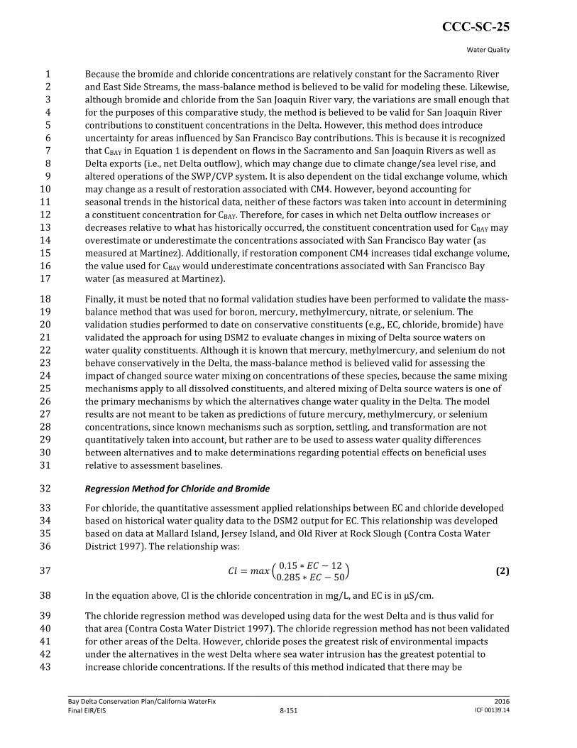
For chloride, the quantitative assessment applied relationships between EC and chloride developed 33 based on historical water quality data to the DSM2 output for EC. This relationship was developed 34 based on data at Mallard Island, Jersey Island, and Old River at Rock Slough (Contra Costa Water 35 District 1997). The relationship was: 36

𝐶𝑙 = 𝑚𝑎𝑥 (0.15 ∗ 𝐸𝐶 − 120.285 ∗ 𝐸𝐶 − 50

) (2) 37

In the equation above, Cl is the chloride concentration in mg/L, and EC is in µS/cm. 38

The chloride regression method was developed using data for the west Delta and is thus valid for 39 that area (Contra Costa Water District 1997). The chloride regression method has not been validated 40 for other areas of the Delta. However, chloride poses the greatest risk of environmental impacts 41 under the alternatives in the west Delta where sea water intrusion has the greatest potential to 42 increase chloride concentrations. If the results of this method indicated that there may be 43

CCC-SC-25

Water Quality



2016 ICF 00139.14

environmental impacts in other areas of the Delta, further assessment was conducted to determine 1 if the method is valid or if another method is more appropriate. 2

For bromide, the same EC to chloride relationship was used, followed by a relationship between 3 chloride and bromide, to estimate bromide concentrations. The chloride to bromide relationship is 4 approximately the same in multiple areas in the west Delta, including Old River at Rock Slough 5 (Contra Costa Water District 1997), the intakes at Banks Pumping Plant (CALFED 2007a), and 6 Mallard Island (Appendix 8E, Bromide, Figure 1). The relationship used was: 7

𝐵𝐵𝐵𝐵 = 0.0035 ∗ 𝑊𝑊𝐶𝐶 (3) 8

In the equation above, Br is the bromide concentration in mg/L, and Cl is the chloride concentration 9 in mg/L.The chloride-to-bromide regression method was developed based on west Delta ratios of 10 chloride to bromide that were indicative of sea-water influence, and so for the purposes of this 11 water quality assessment, is considered valid for that area. However, unlike chloride, bromide 12 concentrations in other areas of the Delta may pose environmental risk. Therefore, in areas outside 13 of the west Delta, further assessment was conducted when this method indicated a potential for 14 environmental risk in order to determine if the method was valid or if another method was more 15 appropriate. 16

Although the regression methods are valid for this water quality assessment where noted above, 17 uncertainty in the results is nonetheless present. The validation studies above describe 18 circumstances in which the model overestimates or underestimates water quality conditions at 19 various locations in the Delta. However, despite this, the methods are still considered valid for 20 comparison purposes as used in this assessment. 21

This alternative to the mass-balance method for calculating bromide and chloride concentrations in 22 the Delta is limited in the sense that the relationships described above are based on historical water 23 quality data that is representative of historical Delta hydrodynamics. It is unknown whether these 24 relationships will still apply in the future with sea-level rise, and particularly under an altered Delta 25 hydrodynamic regime (as would be expected under the action alternatives). Because each of the two 26 methods have limitations and uncertainty, there is no way to determine which method results in 27 more accurate estimates of chloride or bromide. Thus, where applicable (i.e., for west Delta 28 locations), both methods were applied and the results of both methods discussed. In general, when 29 the methods displayed disagreement, impacts were assessed based on the more conservative of the 30 two methods. 31

Both the mass-balance and regression methods include assumptions that limit their ability to 32 accurately account for bromide concentrations that would be likely to occur under project 33 implementation. Some of these include: 34

Projected sea level rise and climate change (i.e., changes in precipitation patterns and 35 snowpack), 36

Inability of the models to account for watershed sources of bromide, 37

Assumed footprint and design of restoration areas, and 38

Simplifications of restoration area geometry necessary to implement in DSM2. 39

CCC-SC-25

Water Quality



2016 ICF 00139.14

Calculation of Use of Assimilative Capacity 1

The concept of assimilative capacity was used as a measure of the extent of water quality 2 degradation that could occur under the alternatives, relative to water quality conditions under the 3 baselines. Water quality degradation was assessed in order to address the Federal and State 4 Antidegradation Policies, which state that existing instream water uses and the level of water quality 5 necessary to protect the existing uses shall be maintained and protected (see Section 8.2.1.3 for a 6 full discussion). Assimilative capacity is the capacity of a water body to experience increased levels 7 of a water quality constituent without exceeding the adopted water quality criterion/objective. In 8 practical terms, when levels or concentrations of a water quality constituent are below water quality 9 criteria/objectives, use of available assimilative capacity by an action is the relative amount of water 10 quality degradation that the action causes (i.e., causing an existing constituent concentration to 11 increase such that its resulting concentration is now closer to, but still below the applicable 12 criterion/objective). If the action causes sufficient degradation of water quality such that the 13 resulting constituent level or concentration is now greater than the criterion/objective, then 100% 14 of the available assimilative capacity would be “used” by the action, and thus no assimilative 15 capacity would remain for that constituent. 16

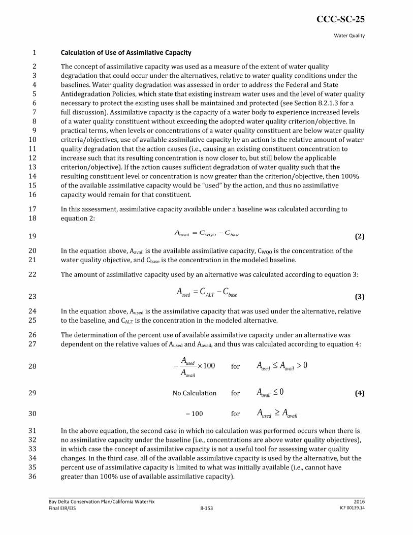
In this assessment, assimilative capacity available under a baseline was calculated according to 17 equation 2: 18

(2) 19

In the equation above, Aavail is the available assimilative capacity, CWQO is the concentration of the 20 water quality objective, and Cbase is the concentration in the modeled baseline. 21

The amount of assimilative capacity used by an alternative was calculated according to equation 3: 22

(3) 23

In the equation above, Aused is the assimilative capacity that was used under the alternative, relative 24 to the baseline, and CALT is the concentration in the modeled alternative. 25

The determination of the percent use of available assimilative capacity under an alternative was 26 dependent on the relative values of Aused and Aavail, and thus was calculated according to equation 4: 27

for 28

No Calculation for (4) 29

– 100 for 30

In the above equation, the second case in which no calculation was performed occurs when there is 31 no assimilative capacity under the baseline (i.e., concentrations are above water quality objectives), 32 in which case the concept of assimilative capacity is not a useful tool for assessing water quality 33 changes. In the third case, all of the available assimilative capacity is used by the alternative, but the 34 percent use of assimilative capacity is limited to what was initially available (i.e., cannot have 35 greater than 100% use of available assimilative capacity). 36

baseWQOavail CCA −=

baseALTused CCA −=

100×−avail

used

AA 0>≤ availused AA

0≤availA

availused AA ≥

CCC-SC-25

Water Quality



2016 ICF 00139.14

Qualitative Assessments 1

Some constituents were assessed strictly qualitatively (Appendix 8C, Screening Analysis, Table SA-2 11) because: 1) insufficient historical monitoring data were available to adequately characterize the 3 concentrations of the five source waters to the Delta (i.e., to accurately define the distribution of 4 concentrations observed in the SAC, SJR, BAY, eastside tributaries, AGR), which are necessary to 5 implement the quantitative mass-balance assessment approach described above; 2) the locations for 6 which the constituent was assessed (within the affected environment) was outside of any available 7 modeling domain, or available modeling tools were not appropriate for predicting constituent 8 concentrations based on the physical, chemical, and/or biological properties and environmental fate 9 and transport of the constituent. Nevertheless, the same conceptual framework was used for 10 qualitatively assessing constituents of concern. Best available information regarding 11 concentrations/levels in the Delta source waters was evaluated relative to how flow-fractions at 12 various Delta locations would change under the alternatives, as defined by DSM2 model flow-13 fraction output (Appendix 8D, Source Water Fingerprinting Results), to estimate the relative 14 frequency and magnitude of change expected for a given constituent at a specified location. 15

Additionally, assessments of the effects of implementing CM2–CM21 were qualitative, at a 16 programmatic level, for all constituents. Construction-related water quality changes also were 17 assessed qualitatively. Potential water quality effects of these generally specific and/or 18 geographically localized actions were assessed by evaluating the anticipated type, duration, and 19 geographic extent of construction activities to take place, and location and type of water bodies 20 potentially affected. The potential for soil, sediment, and contaminants to be discharged to water 21 bodies was determined by identifying construction practices and equipment that could be used, 22 common materials or contaminants that may be present or be used for construction or construction 23 equipment, and pathways by which contaminants may enter receiving waters, and measures to 24 minimize or eliminate adverse construction-related effects on water quality. 25

8.3.1.4 SWP/CVP Export Service Areas 26

Assessment of water quality changes in the SWP/CVP Export Service Areas, which begin at the 27 export pumps (i.e., Banks and Jones pumping plants) and extend to facilities receiving exported 28 Delta water, was conducted for construction-related, operations-related, and restoration-related 29 (CM2–CM21) effects. 30

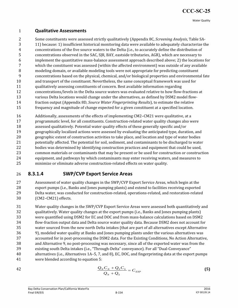
Water quality changes in the SWP/CVP Export Service Areas were assessed both quantitatively and 31 qualitatively. Water quality changes at the export pumps (i.e., Banks and Jones pumping plants) 32 were quantified using DSM2 for EC and DOC and from mass-balance calculations based on DSM2 33 flow-fraction output data and Delta source water quality data. Because DSM2 does not account for 34 water sourced from the new north Delta intakes (that are part of all alternatives except Alternative 35 9), modeled water quality at Banks and Jones pumping plants under the various alternatives was 36 accounted for in post-processing the DSM2 data. For the Existing Conditions, No Action Alternative, 37 and Alternative 9, no post-processing was necessary, since all of the exported water was from the 38 existing south Delta intakes (i.e., “Through-Delta” conveyance). For all “Dual-Conveyance” 39 alternatives (i.e., Alternatives 1A–5, 7, and 8), EC, DOC, and fingerprinting data at the export pumps 40 were blended according to equation 5: 41

(5) 42 EXP

SN

SSNN CQQ

CQCQ=

++

CCC-SC-25

Documents

8.3.1.1 Models Used and Their Linkages - California