826070

Hindawi Publishing CorporationInternational Journal of Aerospace EngineeringVolume 2008, Article ID 826070, 10 pagesdoi:10.1155/2008/826070

Research ArticleTransient Burning Rate Model for Solid Rocket MotorInternal Ballistic Simulations

David R. Greatrix

Department of Aerospace Engineering, Ryerson University, 350 Victoria St., Toronto, Ontario, Canada M5B 2K3

Correspondence should be addressed to David R. Greatrix, [email protected]

Received 8 January 2007; Revised 30 April 2007; Accepted 8 August 2007

Recommended by R. I. Sujith

A general numerical model based on the Zeldovich-Novozhilov solid-phase energy conservation result for unsteady solid-propellant burning is presented in this paper. Unlike past models, the integrated temperature distribution in the solid phase isutilized directly for estimating instantaneous burning rate (rather than the thermal gradient at the burning surface). The burningmodel is general in the sense that the model may be incorporated for various propellant burning-rate mechanisms. Given the avail-ability of pressure-related experimental data in the open literature, varying static pressure is the principal mechanism of interestin this study. The example predicted results presented in this paper are to a substantial extent consistent with the correspondingexperimental firing response data.

Copyright © 2008 David R. Greatrix. This is an open access article distributed under the Creative Commons Attribution License,which permits unrestricted use, distribution, and reproduction in any medium, provided the original work is properly cited.

1. INTRODUCTION

An important aspect in the study of the internal ballistics ofsolid-propellant rocket motors (SRMs) is the ability to un-derstand the behaviour of a given motor under transient con-ditions, that is, beyond what would be considered as quasi-steady or quasiequilibrium conditions. Transient combus-tion and flow conditions arise for example during the igni-tion and chamber filling phase [1–3] prior to nominal quasi-steady operation, during the propellant burnout and cham-ber emptying phase [4, 5] in the latter portion of a motor’sfiring, and on occasion when a motor experiences axial ortransverse combustion instability symptoms [6–9] upon ini-tiation by a disturbance. The simulation of undesirable non-linear axial combustion instability symptoms in SRMs em-ploying cylindrical and noncylindrical propellant grains [10–13] has provided the motivation for the present study.

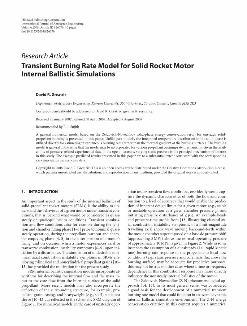
SRM internal ballistic simulation models incorporate al-gorithms for describing the internal flow and the mass in-put to the core flow from the burning surface of the solidpropellant. More recent models may also incorporate thedeflection of the surrounding structure, for example, pro-pellant grain, casing, and heavyweight (e.g., steel) static testsleeve [10–13], as reflected in the schematic SRM diagram ofFigure 1. For numerical models, in the case of unsteady oper-

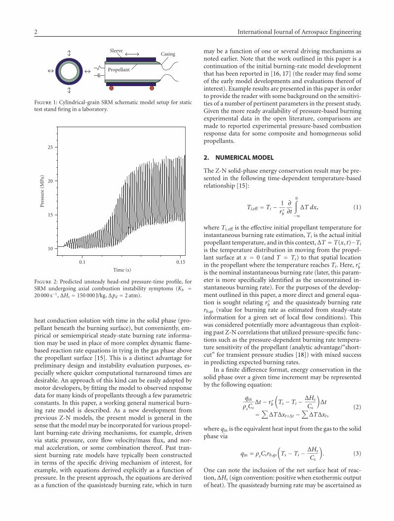
ation under transient flow conditions, one ideally would cap-ture the dynamic characteristics of both the flow and com-bustion to a level of accuracy that would enable the predic-tion of inherent design limits for a given motor (e.g., stableor unstable operation at a given chamber pressure pc andinitiating pressure disturbance of �pd). An example head-end pressure-time profile from [13] illustrating classical ax-ial combustion instability symptoms, of a limit-magnitudetravelling axial shock wave moving back-and-forth withinthe motor chamber superimposed on a base dc pressure shift(approaching 5 MPa) above the normal operating pressureof approximately 10 MPa, is given in Figure 2. While in someinstances the assumption of a quasisteady (i.e., rapid kineticrate) burning rate response of the propellant to local flowconditions (e.g., static pressure and core mass flux above theburning surface) may be adequate for predictive purposes,this may not be true in other cases where a time or frequencydependence in this combustion response may more directlyinfluence the nonsteady internal ballistics of the motor.

The Zeldovich-Novozhilov (Z-N) phenomenological ap-proach [14, 15], in its most general sense, was considereda good basis for the development of a numerical transientburning rate model that could function in an overall dynamicinternal ballistic simulation environment. The Z-N energyconservation criterion in this context requires a numerical

2 International Journal of Aerospace Engineering

SleeveCasing

Propellant

Figure 1: Cylindrical-grain SRM schematic model setup for statictest stand firing in a laboratory.

10

15

20

25

Pre

ssu

re(M

Pa)

0.1 0.15

Time (s)

Figure 2: Predicted unsteady head-end pressure-time profile, forSRM undergoing axial combustion instability symptoms (Kb =20 000 s−1, ΔHs = 150 000 J/kg, Δpd = 2 atm).

heat conduction solution with time in the solid phase (pro-pellant beneath the burning surface), but conveniently, em-pirical or semiempirical steady-state burning rate informa-tion may be used in place of more complex dynamic flame-based reaction rate equations in tying in the gas phase abovethe propellant surface [15]. This is a distinct advantage forpreliminary design and instability evaluation purposes, es-pecially where quicker computational turnaround times aredesirable. An approach of this kind can be easily adopted bymotor developers, by fitting the model to observed responsedata for many kinds of propellants through a few parametricconstants. In this paper, a working general numerical burn-ing rate model is described. As a new development fromprevious Z-N models, the present model is general in thesense that the model may be incorporated for various propel-lant burning-rate driving mechanisms, for example, drivenvia static pressure, core flow velocity/mass flux, and nor-mal acceleration, or some combination thereof. Past tran-sient burning rate models have typically been constructedin terms of the specific driving mechanism of interest, forexample, with equations derived explicitly as a function ofpressure. In the present approach, the equations are derivedas a function of the quasisteady burning rate, which in turn

may be a function of one or several driving mechanisms asnoted earlier. Note that the work outlined in this paper is acontinuation of the initial burning-rate model developmentthat has been reported in [16, 17] (the reader may find someof the early model developments and evaluations thereof ofinterest). Example results are presented in this paper in orderto provide the reader with some background on the sensitivi-ties of a number of pertinent parameters in the present study.Given the more ready availability of pressure-based burningexperimental data in the open literature, comparisons aremade to reported experimental pressure-based combustionresponse data for some composite and homogeneous solidpropellants.

2. NUMERICAL MODEL

The Z-N solid-phase energy conservation result may be pre-sented in the following time-dependent temperature-basedrelationship [15]:

Ti,eff = Ti − 1r∗b

∂

∂t

0∫

−∞ΔT dx, (1)

where Ti, eff is the effective initial propellant temperature forinstantaneous burning rate estimation, Ti is the actual initialpropellant temperature, and in this context,ΔT = T(x, t)−Tiis the temperature distribution in moving from the propel-lant surface at x = 0 (and T = Ts) to that spatial locationin the propellant where the temperature reaches Ti. Here, r∗bis the nominal instantaneous burning rate (later, this param-eter is more specifically identified as the unconstrained in-stantaneous burning rate). For the purposes of the develop-ment outlined in this paper, a more direct and general equa-tion is sought relating r∗b and the quasisteady burning raterb,qs (value for burning rate as estimated from steady-stateinformation for a given set of local flow conditions). Thiswas considered potentially more advantageous than exploit-ing past Z-N correlations that utilized pressure-specific func-tions such as the pressure-dependent burning rate tempera-ture sensitivity of the propellant (analytic advantage/“short-cut” for transient pressure studies [18]) with mixed successin predicting expected burning rates.

In a finite difference format, energy conservation in thesolid phase over a given time increment may be representedby the following equation:

qin

ρsCsΔt − r∗b

(Ts − Ti − ΔHs

Cs

)Δt

=∑ΔTΔxt+Δt −

∑ΔTΔxt,

(2)

where qin is the equivalent heat input from the gas to the solidphase via

qin = ρsCsrb,qs

(Ts − Ti − ΔHs

Cs

). (3)

One can note the inclusion of the net surface heat of reac-tion,ΔHs (sign convention: positive when exothermic outputof heat). The quasisteady burning rate may be ascertained as

David R. Greatrix 3

a function of such parameters as static pressure of the localflow, for example through de St. Robert’s law [5]:

rb,qs(p) = Cpn. (4)

Through substitution, one arrives at

r∗b = rb,qs −∑ΔTΔxt+Δt −

∑ΔTΔxt(

Ts − Ti − ΔHs/Cs)Δt

(5)

which conforms to

r∗b = rb,qs − 1(Ts − Ti − ΔHs/Cs

) ∂∂t

0∫

−∞ΔTdx. (6)

In (6), r∗b is the nominal (unconstrained) instantaneousburning rate, and its value at a given propellant grain lo-cation is solved at each time increment via numerical in-tegration of the temperature distribution through the heatpenetration zone of the solid phase. In this respect, thepresent numerical model differs from past numerical mod-els, for example, as reported by Kooker and Nelson [19].In those past cases, the thermal gradient at the propellantsurface (∂T/∂x|x=0) was explicitly tied to the true instanta-neous burning rate rb by a specified function, and in turn,rb commonly tied to a variable surface temperature Ts by anArrhenius-type expression [18]. In following this establishedtrend, earlier versions of numerical Z-N models did not fol-low through on using (6) directly, but switched to a burningrate temperature sensitivity correlation such as [18, 20]

∂T

∂x

∣∣∣∣x=0

= rbαs

[Ts − 1

σ pln(rbrb,qs

)− Ti

], (7)

where σ p is the pressure-based burning rate temperature sen-sitivity [20]. As reported by Nelson [18], the predicted rbaugmentation using (7) was commonly lower than expectedfrom experimental observation, for a number of transientburning applications, and relative to various flame-based ex-pressions for thermal surface gradient as a function of rb, ofthe general form [18]

∂T

∂x

∣∣∣∣x=0

= g1rb +g2

rb. (8)

The coefficients g1 and g2 may be found as a function of anumber of fixed and variable parameters [18], depending onthe given model being employed.

Returning to the present model, in the solid phase, thetransient heat conduction is governed by [14, 21]

ks∂2T

∂x2= ρsCs

∂T

∂t. (9)

In finite difference format (in this example, for first-order ac-curacy in time), the temperature at a given internal locationmay be presented as

Tt+Δt,x = Tt,x + αsΔt(Δx)2

[Tt,x−Δx − 2Tt,x + Tt,x+Δx

]. (10)

For a first-order explicit scheme, note that the Fourier stabil-ity requirement stipulates that [21]

αsΔt(Δx)2 ≤

12. (11)

While a fourth-order Runge-Kutta scheme was adopted forthe present work, the above criterion does prove useful as aguideline. Note that a time step of 1 × 10−7 seconds has beenchosen as the reference value for this investigation, based onprevious SRM simulation studies [10–13]. The correspond-ing spatial step Δx would typically be set to the Fourier sta-bility requirement limit, namely ΔxFo = (2αs Δt)

1/2.Allowing for the propellant’s surface regression of rbΔt

with each time step, where rb is the true instantaneous rateof regression, and maintaining the surface position as x =0 relative to spatial nodes deeper in the propellant, a givennode’s temperature may be updated via

Tt,x+rbΔt = Tt,x − Tt,x−Δx − Tt,xΔx

(rbΔt

). (12)

The boundary condition at the propellant surface (x = 0,T = Ts) to first-order accuracy may be applied through

Tt+Δt,−Δx = Tt,−Δx +Δt

ρsCsΔx

×[ks(Tt,−2Δx − Tt,−Δx

)Δx

+ks(Ts − Tt,−Δx

)Δx

+ Δqeff

],

(13)

where Δqeff represents the net heat input from the gas phaseinto the regressing solid (this parameter will be discussed inmore detail later in the paper).

With respect to the burning surface temperature Ts, onehas the option of treating it as constant, or allowing for itsvariation, depending on the phenomenological approach be-ing taken for estimating the burning rate. In the past, it wasnot uncommon to encounter estimation models assuming amean or constant Ts. More recently, usage of an Arrheniusrelation for solid pyrolysis dictating a variable Ts has becomemore prevalent [14, 18].

The numerical model, as described above and with apreliminary assumption of a constant Ts, is unstable (solu-tion for transient r∗b being strongly divergent), using exam-ple propellant properties comparable to Propellant A (seeTable 1; nonaluminized ammonium perchlorate/hydroxyl-terminated polybutadiene [AP/HTPB] composite), and overa range of different time and spatial increment sizes [16].An additional equation limiting the transition of the instan-taneous burning rate rb with time is required to physicallyconstrain the model. From the author’s previous backgroundin general numerical modeling where lagging a parameter’svalue is a desired objective, a simple empirical means for ap-plying this constraint is as follows:

drbdt

= Kb(r∗b − rb

). (14)


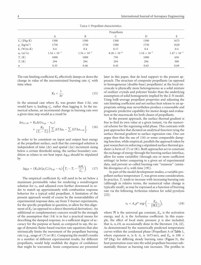
Table 1: Propellant characteristics.

Propellants

A B C D E

Cs (J/kg-K) 1500 1500 1300 1500 1675

ρs (kg/m3) 1730 1730 1580 1730 1620

ks (W/m-K) 0.4 0.4 0.17 0.4 0.4

αs (m2/s) 1.54 × 10−7 1.54 × 10−7 8.28 × 10−8 1.54 × 10−7 1.47 × 10−7

Ts (K) 1000 1000 750 1000 650

Ti (K) 294 294 294 294 300

n 0.35 0.46 0.45 0.65 0.69

The rate limiting coefficientKb effectively damps or slows thechange in value of the unconstrained burning rate r∗b withtime when

Kb <1Δt. (15)

In the unusual case where Kb was greater than 1/Δt, onewould have rb leading r∗b , rather than lagging it. In the nu-merical scheme, an incremental change in burning rate overa given time step would as a result be

Δrb,t+Δt = KbΔt(rb,qs − rb,t

)

+Kb(

Ts − Ti)[∑

ΔTΔxt −∑ΔTΔxt+Δt

].

(16)

In order to be consistent on input and output heat energyat the propellant surface, such that the converged solution isindependent of time (Δt) and spatial (Δx) increment sizingbelow a certain threshold sizing, the surface boundary con-dition as relates to net heat input Δqeff should be stipulatedby

Δqeff =(KbΔt

)ρsCs

(rb,qs − rb

)(Ts − Ti − ΔHs

Cs

). (17)

The empirical coefficient Kb will need to be set below amaximum permissible value for rendering a nondivergentsolution for rb, and adjusted even further downward in or-der to match up approximately with combustion responsebehavior for a typical solid propellant. A limitation of thepresent approach would of course be the nonavailability ofexperimental response data, say from T-burner experiments,for the specific propellant in question, to allow for this align-ment ofKb (as opposed to a direct theoretical derivation). Anadditional or complementary concern would be the strengthof the assumption that (14) is in fact a practical means fordescribing the damped response, to a sufficient degree of ac-curacy for the purpose at hand, as compared to say, the us-age of dynamic flame-based reaction rate equations that alsointrinsically limits the movement of the propellant burningrate (e.g., usage of (7) or (8)). Comparing the model’s resultsto a number of different experimental results, for differentpropellants, would help establish the degree of confidencethat might be warranted. Some comparisons are presented

later in this paper, that do lend support to the present ap-proach. The structure of composite propellants (as opposedto homogeneous [double-base] propellants) at the local mi-croscale is physically more heterogeneous as a solid mixtureof oxidizer crystals and polymer binder than the underlyingassumption of solid homogeneity implied by the Z-N model.Using bulk-average propellant properties and adjusting therate limiting coefficient and net surface heat release to an ap-propriate setting may nevertheless produce a reasonable andpragmatic predictive capability for motor design and evalua-tion at the macroscale for both classes of propellants.

In the present approach, the surface thermal gradient isfree to find its own value at a given instant, via the numeri-cal scheme for the regressing solid phase. This contrasts withpast approaches that dictated an analytical function tying thesurface thermal gradient to surface regression rate. One canargue then that the use of (14) or some comparable damp-ing function, while empirical, parallels the approach taken bypast researchers in enforcing a stipulated surface thermal gra-dient (a form of (7) or (8)). Both approaches act to constrainthe exchange of energy through the burning surface interface,allow for some variability (through one or more coefficientsettings) in better comparing to a given set of experimentaldata, and prevent so-called burning-rate “runaway” (unsta-ble divergence of rb with time [19]).

As part of the model development studies, a variable pro-pellant surface temperature Ts was given some consideration.In practice, Ts tends to increase with increasing burning rate(although in relative terms, the numerical value change istypically small), as may be expressed as a function of burningrate via the following Arrhenius relation for solid pyrolysis[22]:

rb = Aspns exp

(− Eas[

RTs])

, (18)

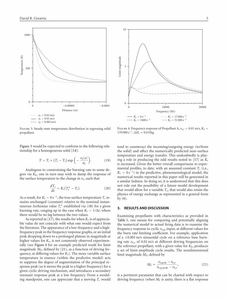
where R is the universal gas constant, Eas is the activationenergy, and As is the Arrhenius coefficient. In this exam-ple, the effect of local static pressure p is also included,that is, ns �=0, as occasionally done in the literature [14, 22].As demonstrated by the numerically predicted temperaturecurves within the condensed phase (Propellant A of Table 1,where exponent ns is 0, As is 1675 m/s, and Eas is 100 ×106 J/kg) for differing steady burning rates (Figure 3), theheat penetration zone into the solid propellant becomes sub-stantially thinner as burning rate increases. The profiles in

David R. Greatrix 5

0

500

1000

Tem

per

atu

re(K

)

0 −0.00005 −0.0001

Distance (m)

rb = 0.02 m/srb = 0.01 m/srb = 0.005 m/s

Figure 3: Steady-state temperature distribution in regressing solidpropellant.

Figure 3 would be expected to conform to the following rela-tionship for a homogeneous solid [14]:

T = Ti +(Ts − Ti

)exp

(− rb|x|

αs

). (19)

Analogous to constraining the burning rate to some de-gree via Kb, one in turn may wish to damp the response ofthe surface temperature to the change in rb, such that

dTsdt

= Kt(T∗s − Ts

). (20)

As a result, for Kt = 0 s−1, the true surface temperature Ts re-mains unchanged (constant) relative to the nominal instan-taneous Arrhenius value T∗s established via (18) for a givenburning rate, ranging up to the case when Kt = 1/Δt, wherethere would be no lag between the two values.

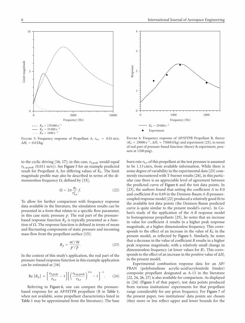
As reported in [17], the results for whenKt is of apprecia-ble value do not coincide with what one would expect fromthe literature. The appearance of a low-frequency and a high-frequency peak in the frequency response graphs, or an initialpeak dropping down to a prolonged plateau in magnitude athigher values for Kt, is not commonly observed experimen-tally (see Figure 4 for an example predicted result for limitmagnitude M� , defined by (21), as a function of driving fre-quency, at differing values for Kt). The more variable surfacetemperature in essence (within the predictive model) actsto suppress the degree of augmentation of the principal re-sponse peak (as it moves the peak to a higher frequency) for agiven cyclic driving mechanism, and introduces a secondaryresonant response peak at a low frequency. From a model-ing standpoint, one can appreciate that a moving Ts would

0

5

10

Lim

itm

agn

itu

de

0 10000 20000

Frequency (Hz)

Kt = 0 s−1

Kt = 3400 s−1Kt = 17 000 s−1

Kt = 51 000 s−1

Figure 4: Frequency response of Propellant A, rb,o = 0.01 m/s, Kb =170 000 s−1, ΔHs = 0.0 J/kg.

tend to counteract the incoming/outgoing energy (to/fromthe solid) and affect the numerically predicted near-surfacetemperature and energy transfer. This undoubtedly is play-ing a role in producing the odd results noted in [17] as Ktis increased. Given the better overall comparisons to exper-imental profiles, to date, with an assumed constant Ts (i.e.,Kt = 0 s−1) in the predictive, phenomenological model, thenumerical results reported in this paper will be generated ina similar fashion. In doing so, it is understood that this doesnot rule out the possibility of a future model developmentthat would allow for a variable Ts, that would also retain thephysics of energy exchange as represented in a general formby (6).

3. RESULTS AND DISCUSSION

Examining propellants with characteristics as provided inTable 1, one means for comparing and potentially aligningthe numerical model to actual firing data is to examine thefrequency response to cyclic rb,qs input, at different values forthe burn rate limiting coefficient. For example, applicationof a ±0.001 m/s sinusoidal cycle on a reference base burn-ing rate rb,o of 0.01 m/s at different driving frequencies onthe reference propellant, with a given value for Kb, producesa set of limit-amplitude cycle results. The nondimensionallimit magnitude M� , defined by

M� =rb,peak − rb,o

rb,qs,peak − rb,o, (21)

is a pertinent parameter that can be charted with respect todriving frequency (when M� is unity, there is a flat response


0

5

10

Lim

itm

agn

itu

de

0 5000 10000

Frequency (Hz)

Kb = 170 000 s−1

Kb = 35 000 s−1

Kb = 1600 s−1

Figure 5: Frequency response of Propellant A, rb,o = 0.01 m/s,ΔHs = 0.0 J/kg.

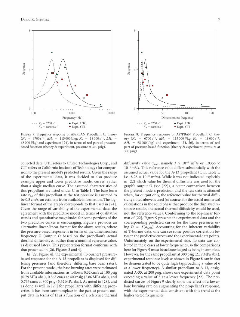
to the cyclic driving [16, 17]; in this case, rb,peak would equalrb, qs,peak (0.011 m/s)). See Figure 5 for an example predictedresult for Propellant A, for differing values of Kb. The limitmagnitude profile may also be described in terms of the di-mensionless frequency Ω, defined by [15],

Ω = 2παsr2b,o

f . (22)

To allow for further comparison with frequency responsedata available in the literature, the simulation results can bepresented in a form that relates to a specific flow parameter,in this case static pressure p. The real part of the pressure-based response function Rp is typically presented as a func-tion of Ω. The response function is defined in terms of meanand fluctuating components of static pressure and incomingmass flow from the propellant surface [15]:

Rp = m′/ mp′/ p

. (23)

In the context of this study’s application, the real part of thepressure-based response function in this example applicationcan be estimated as [16]

Re{Rp} =

[rb,peak

rb,o− 1][(

rb,qs,peak

rb,o

)1/n

− 1]−1

. (24)

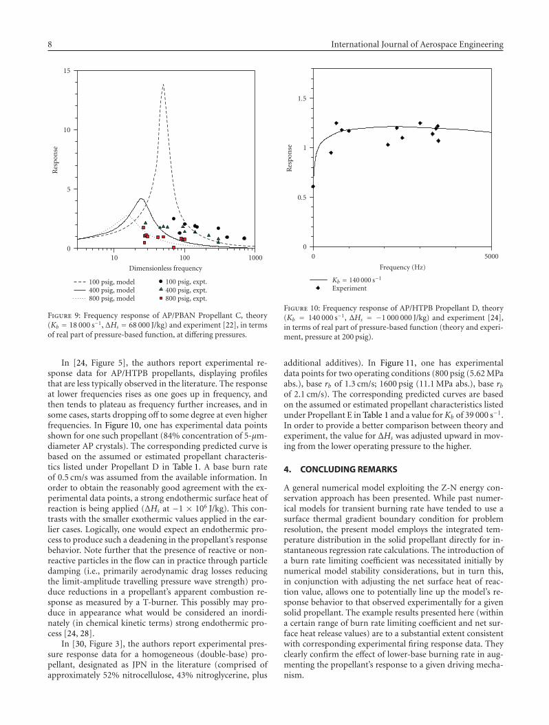
Referring to Figure 6, one can compare the pressure-based response for an AP/HTPB propellant (B in Table 1;when not available, some propellant characteristics listed inTable 1 may be approximated from the literature). The base

0

1

2

3

4

Res

pon

se

0 1000 2000

Frequency (Hz)

Kb = 29 000 s−1

Experiment

Figure 6: Frequency response of AP/HTPB Propellant B, theory(Kb = 29000 s−1, ΔHs = 75000 J/kg) and experiment [23], in termsof real part of pressure-based function (theory & experiment, pres-sure at 1200 psig).

burn rate rb,o of this propellant at the test pressure is assumedto be 1.13 cm/s, from available information. While there issome degree of variability in the experimental data [23] com-monly encountered with T-burner results [24], in this partic-ular case there is an appreciable level of agreement betweenthe predicted curve of Figure 6 and the test data points. In[23], the authors found that setting the coefficient A to 8.0and coefficient B to 0.69 in the Denison-Baum A-B pressure-coupled response model [22] produced a relatively good fit tothe available test data points (the Denison-Baum predictedcurve is quite similar to the present model’s curve). In Co-hen’s study of the application of the A-B response modelto homogeneous propellants [25], he notes that an increasein value for coefficient A results in a higher peak responsemagnitude, at a higher dimensionless frequency. This corre-sponds to the effect of an increase in the value of Kb in thepresent model, as reflected by Figure 5. Similarly, he notesthat a decrease in the value of coefficient B results in a higherpeak response magnitude, with a relatively small change indimensionless frequency (at lower values for B). This corre-sponds to the effect of an increase in the positive value ofΔHs

in the present model.Experimental combustion response data for an AP/

PBAN (polybutadiene acrylic-acid/acrylonitrile binder)composite propellant designated as A-13 in the literature[22, 24, 26, 27] is also available for comparison. As displayedin [24] (Figure 3 of that paper), test data points producedfrom various institutions’ experiments for that propellantrange considerably for any given frequency. For Figure 7 ofthe present paper, two institutions’ data points are chosen(they more or less reflect upper and lower bounds for the

David R. Greatrix 7

0

4

8

Res

pon

se

100 1000 10000

Frequency (Hz)

Kb = 6700 s−1

Kb = 18 000 s−1Expt., UTCExpt., CIT

Figure 7: Frequency response of AP/PBAN Propellant C, theory(Kb = 6700 s−1, ΔHs = 115 000 J/kg; Kb = 18 000 s−1, ΔHs =68 000 J/kg) and experiment [24], in terms of real part of pressure-based function (theory & experiment, pressure at 300 psig).

collected data; UTC refers to United Technologies Corp., andCIT refers to California Institute of Technology) for compar-ison to the present model’s predicted results. Given the rangeof the experimental data, it was decided to also produceexample upper and lower predictive model curves, ratherthan a single median curve. The assumed characteristics ofthis propellant are listed under C in Table 1. The base burnrate rb,o of this propellant at the test pressure is assumed tobe 0.5 cm/s, an estimate from available information. The log-linear format of the graph corresponds to that used in [24].Given the range of variability of the experimental data, theagreement with the predictive model in terms of qualitativetrends and quantitative magnitudes for some portions of thetwo predictive curves is encouraging. Figure 8 provides analternative linear-linear format for the above results, wherethe pressure-based response is in terms of the dimensionlessfrequency Ω (output Ω based on the propellant’s actualthermal diffusivity αs, rather than a nominal reference value,as discussed later). This presentation format conforms withthat presented in [26, Figures 3 and 4].

In [22, Figure 4], the experimental (T-burner) pressure-based response for the A-13 propellant is displayed for dif-fering pressures (and therefore, differing base burn rates).For the present model, the base burning rates were estimatedfrom available information, as follows: 0.32 cm/s at 100 psig(0.79 MPa abs.), 0.565 cm/s at 400 psig (2.86 MPa abs.), and0.766 cm/s at 800 psig (5.62 MPa abs.). As noted in [28], andas done as well in [29] for propellants with differing prop-erties, it has been commonplace in the past to present out-put data in terms of Ω as a function of a reference thermal

0

4

8

Res

pon

se

0 50 100 150

Dimensionless frequency

Kb = 6700 s−1

Kb = 18 000 s−1Expt., UTCExpt., CIT

Figure 8: Frequency response of AP/PBAN Propellant C, the-ory (Kb = 6700 s−1, ΔHs = 115 000 J/kg; Kb = 18 000 s−1,ΔHs = 68 000 J/kg) and experiment [24, 26], in terms of realpart of pressure-based function (theory & experiment, pressure at300 psig).

diffusivity value αs,ref, namely 3 × 10−4 in2/s or 1.9355 ×10−7m2/s. This reference value differs substantially with theassumed actual value for the A-13 propellant (C in Table 1,i.e., 8.28 × 10−8 m2/s). While it was not indicated explicitlyin [22] which value for thermal diffusivity was used for thegraph’s output Ω (see (22)), a better comparison betweenthe present model’s prediction and the test data is attainedwhen, for output only, the reference value for thermal diffu-sivity noted above is used (of course, for the actual numericalcalculations in the solid phase that produce the displayed re-sponse results, the actual thermal diffusivity would be used,not the reference value). Conforming to the log-linear for-mat of [22], Figure 9 presents the experimental data and thecorresponding predicted curves for the three pressures us-ing Ω = f (αs,ref). Accounting for the inherent variabilityof T-burner data, one can see some positive correlation be-tween the predictive curves and the experimental data points.Unfortunately, on the experimental side, no data was col-lected in these cases at lower frequencies, so the comparisonshere for Figure 9 must be acknowledged as being incomplete.However, for the same propellant at 300 psig (2.17 MPa abs.),experimental response levels as shown in Figure 8 can in factbe demonstrated to be quite high (approaching a value of 6at a lower frequency). A similar propellant to A-13, desig-nated A-35, at 200 psig, shows one experimental data pointexceeding a value of 5 at a lower frequency [22]. The pre-dicted curves of Figure 9 clearly show the effect of a lower-base burning rate on augmenting the propellant’s response,with the experimental data consistent with this trend at thehigher tested frequencies.


0

5

10

15

Res

pon

se

10 100 1000

Dimensionless frequency

100 psig, model400 psig, model800 psig, model

100 psig, expt.400 psig, expt.800 psig, expt.

Figure 9: Frequency response of AP/PBAN Propellant C, theory(Kb = 18 000 s−1, ΔHs = 68 000 J/kg) and experiment [22], in termsof real part of pressure-based function, at differing pressures.

In [24, Figure 5], the authors report experimental re-sponse data for AP/HTPB propellants, displaying profilesthat are less typically observed in the literature. The responseat lower frequencies rises as one goes up in frequency, andthen tends to plateau as frequency further increases, and insome cases, starts dropping off to some degree at even higherfrequencies. In Figure 10, one has experimental data pointsshown for one such propellant (84% concentration of 5-μm-diameter AP crystals). The corresponding predicted curve isbased on the assumed or estimated propellant characteris-tics listed under Propellant D in Table 1. A base burn rateof 0.5 cm/s was assumed from the available information. Inorder to obtain the reasonably good agreement with the ex-perimental data points, a strong endothermic surface heat ofreaction is being applied (ΔHs at −1 × 106 J/kg). This con-trasts with the smaller exothermic values applied in the ear-lier cases. Logically, one would expect an endothermic pro-cess to produce such a deadening in the propellant’s responsebehavior. Note further that the presence of reactive or non-reactive particles in the flow can in practice through particledamping (i.e., primarily aerodynamic drag losses reducingthe limit-amplitude travelling pressure wave strength) pro-duce reductions in a propellant’s apparent combustion re-sponse as measured by a T-burner. This possibly may pro-duce in appearance what would be considered an inordi-nately (in chemical kinetic terms) strong endothermic pro-cess [24, 28].

In [30, Figure 3], the authors report experimental pres-sure response data for a homogeneous (double-base) pro-pellant, designated as JPN in the literature (comprised ofapproximately 52% nitrocellulose, 43% nitroglycerine, plus

0

0.5

1

1.5

Res

pon

se

0 5000

Frequency (Hz)

Kb = 140 000 s−1

Experiment

Figure 10: Frequency response of AP/HTPB Propellant D, theory(Kb = 140 000 s−1, ΔHs = −1 000 000 J/kg) and experiment [24],in terms of real part of pressure-based function (theory and experi-ment, pressure at 200 psig).

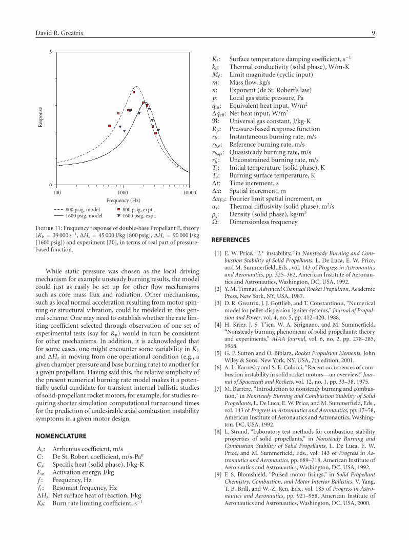
additional additives). In Figure 11, one has experimentaldata points for two operating conditions (800 psig (5.62 MPaabs.), base rb of 1.3 cm/s; 1600 psig (11.1 MPa abs.), base rbof 2.1 cm/s). The corresponding predicted curves are basedon the assumed or estimated propellant characteristics listedunder Propellant E in Table 1 and a value forKb of 39 000 s−1.In order to provide a better comparison between theory andexperiment, the value for ΔHs was adjusted upward in mov-ing from the lower operating pressure to the higher.

4. CONCLUDING REMARKS

A general numerical model exploiting the Z-N energy con-servation approach has been presented. While past numer-ical models for transient burning rate have tended to use asurface thermal gradient boundary condition for problemresolution, the present model employs the integrated tem-perature distribution in the solid propellant directly for in-stantaneous regression rate calculations. The introduction ofa burn rate limiting coefficient was necessitated initially bynumerical model stability considerations, but in turn this,in conjunction with adjusting the net surface heat of reac-tion value, allows one to potentially line up the model’s re-sponse behavior to that observed experimentally for a givensolid propellant. The example results presented here (withina certain range of burn rate limiting coefficient and net sur-face heat release values) are to a substantial extent consistentwith corresponding experimental firing response data. Theyclearly confirm the effect of lower-base burning rate in aug-menting the propellant’s response to a given driving mecha-nism.

David R. Greatrix 9

0

5

Res

pon

se

100 1000 10000

Frequency (Hz)

800 psig, model1600 psig, model

800 psig, expt.1600 psig, expt.

Figure 11: Frequency response of double-base Propellant E, theory(Kb = 39 000 s−1, ΔHs = 45 000 J/kg [800 psig], ΔHs = 90 000 J/kg[1600 psig]) and experiment [30], in terms of real part of pressure-based function.

While static pressure was chosen as the local drivingmechanism for example unsteady burning results, the modelcould just as easily be set up for other flow mechanismssuch as core mass flux and radiation. Other mechanisms,such as local normal acceleration resulting from motor spin-ning or structural vibration, could be modeled in this gen-eral scheme. One may need to establish whether the rate lim-iting coefficient selected through observation of one set ofexperimental tests (say for Rp) would in turn be consistentfor other mechanisms. In addition, it is acknowledged thatfor some cases, one might encounter some variability in Kband ΔHs in moving from one operational condition (e.g., agiven chamber pressure and base burning rate) to another fora given propellant. Having said this, the relative simplicity ofthe present numerical burning rate model makes it a poten-tially useful candidate for transient internal ballistic studiesof solid-propellant rocket motors, for example, for studies re-quiring shorter simulation computational turnaround timesfor the prediction of undesirable axial combustion instabilitysymptoms in a given motor design.

NOMENCLATURE

As: Arrhenius coefficient, m/sC: De St. Robert coefficient, m/s-Pan

Cs: Specific heat (solid phase), J/kg-KEas Activation energy, J/kgf : Frequency, Hzfr : Resonant frequency, HzΔHs: Net surface heat of reaction, J/kgKb: Burn rate limiting coefficient, s−1

Kt: Surface temperature damping coefficient, s−1

ks: Thermal conductivity (solid phase), W/m-KM� : Limit magnitude (cyclic input)m: Mass flow, kg/sn: Exponent (de St. Robert’s law)p: Local gas static pressure, Paqin: Equivalent heat input, W/m2

Δqeff: Net heat input, W/m2

R: Universal gas constant, J/kg-KRp: Pressure-based response functionrb: Instantaneous burning rate, m/srb,o: Reference burning rate, m/srb,qs: Quasisteady burning rate, m/sr∗b : Unconstrained burning rate, m/sTi: Initial temperature (solid phase), KTs: Burning surface temperature, KΔt: Time increment, sΔx: Spatial increment, mΔxFo: Fourier limit spatial increment, mαs: Thermal diffusivity (solid phase), m2/sρs: Density (solid phase), kg/m3

Ω: Dimensionless frequency

REFERENCES

[1] E. W. Price, “L∗ instability,” in Nonsteady Burning and Com-bustion Stability of Solid Propellants, L. De Luca, E. W. Price,and M. Summerfield, Eds., vol. 143 of Progress in Astronauticsand Aeronautics, pp. 325–362, American Institute of Aeronau-tics and Astronautics, Washington, DC, USA, 1992.

[2] Y. M. Timnat, Advanced Chemical Rocket Propulsion, AcademicPress, New York, NY, USA, 1987.

[3] D. R. Greatrix, J. J. Gottlieb, and T. Constantinou, “Numericalmodel for pellet-dispersion igniter systems,” Journal of Propul-sion and Power, vol. 4, no. 5, pp. 412–420, 1988.

[4] H. Krier, J. S. T’ien, W. A. Sirignano, and M. Summerfield,“Nonsteady burning phenomena of solid propellants: theoryand experiments,” AIAA Journal, vol. 6, no. 2, pp. 278–285,1968.

[5] G. P. Sutton and O. Biblarz, Rocket Propulsion Elements, JohnWiley & Sons, New York, NY, USA, 7th edition, 2001.

[6] A. L. Karnesky and S. E. Colucci, “Recent occurrences of com-bustion instability in solid rocket motors—an overview,” Jour-nal of Spacecraft and Rockets, vol. 12, no. 1, pp. 33–38, 1975.

[7] M. Barrere, “Introduction to nonsteady burning and combus-tion,” in Nonsteady Burning and Combustion Stability of SolidPropellants, L. De Luca, E. W. Price, and M. Summerfield, Eds.,vol. 143 of Progress in Astronautics and Aeronautics, pp. 17–58,American Institute of Aeronautics and Astronautics, Washing-ton, DC, USA, 1992.

[8] L. Strand, “Laboratory test methods for combustion-stabilityproperties of solid propellants,” in Nonsteady Burning andCombustion Stability of Solid Propellants, L. De Luca, E. W.Price, and M. Summerfield, Eds., vol. 143 of Progress in As-tronautics and Aeronautics, pp. 689–718, American Institute ofAeronautics and Astronautics, Washington, DC, USA, 1992.

[9] F. S. Blomshield, “Pulsed motor firings,” in Solid PropellantChemistry, Combustion, and Motor Interior Ballistics, V. Yang,T. B. Brill, and W.-Z. Ren, Eds., vol. 185 of Progress in Astro-nautics and Aeronautics, pp. 921–958, American Institute ofAeronautics and Astronautics, Washington, DC, USA, 2000.


[10] S. Loncaric, D. R. Greatrix, and Z. Fawaz, “Star-grain rocketmotor—nonsteady internal ballistics,” Aerospace Science andTechnology, vol. 8, no. 1, pp. 47–55, 2004.

[11] D. R. Greatrix, “Nonsteady interior ballistics of cylindrical-grain solid rocket motors,” in Proceedings of the 2nd Inter-national Conference on Computational Ballistics, pp. 281–289,WIT Press, Cordoba, Spain, May 2005.

[12] J. Montesano, D. R. Greatrix, K. Behdinan, and Z. Fawaz,“Structural oscillation considerations for solid rocket in-ternal ballistics modeling,” in Proceedings of the 41stAIAA/ASME/SAE/ASEE Joint Propulsion Conference and Ex-hibit, Tucson, Ariz, USA, July 2005, AIAA 2005-4161.

[13] D. R. Greatrix, “Predicted nonsteady internal ballisticsof cylindrical-grain motor,” in Proceedings of the 42ndAIAA/ASME/SAE/ASEE Joint Propulsion Conference and Ex-hibit, Sacramento, Calif, USA, July 2006, AIAA 2006-4427.

[14] B. V. Novozhilov, “Theory of nonsteady burning and com-bustion instability of solid propellants by the Zeldovich-Novozhilov method,” in Nonsteady Burning and CombustionStability of Solid Propellants, L. De Luca, E. W. Price, and M.Summerfield, Eds., vol. 143 of Progress in Astronautics andAeronautics, pp. 601–642, American Institute of Aeronauticsand Astronautics, Washington, DC, USA, 1992.

[15] M. Q. Brewster, “Solid propellant combustion response: quasi-steady (QSHOD) theory development and validation,” in SolidPropellant Chemistry, Combustion, and Motor Interior Ballis-tics, V. Yang, T. B. Brill, and W.-Z. Ren, Eds., vol. 185 of Progressin Astronautics and Aeronautics, pp. 607–638, American Insti-tute of Aeronautics and Astronautics, Washington, DC, USA,2000.

[16] D. R. Greatrix, “Numerical transient burning rate model forsolid rocket motor simulations,” in Proceedings of the 40thAIAA/ASME/SAE/ASEE Joint Propulsion Conference and Ex-hibit, Fort Lauderdale, Fla, USA, July 2004, AIAA 2004-3726.

[17] D. R. Greatrix, “Numerical modeling considerations for tran-sient burning of solid propellants,” in Proceedings of the 41stAIAA/ASME/SAE/ASEE Joint Propulsion Conference and Ex-hibit, Tucson, Ariz, USA, July 2005, AIAA 2005-4005.

[18] C. W. Nelson, “Response of three types of transient combus-tion models to gun pressurization,” Combustion and Flame,vol. 32, pp. 317–319, 1978.

[19] D. E. Kooker and C. W. Nelson, “Numerical solution of solidpropellant transient combustion,” Journal of Heat Transfer,vol. 101, no. 2, pp. 359–364, 1979.

[20] K. K. Kuo, S. Kumar, and B. Zhang, “Transient burn-ing characteristics of JA2 propellant using experimentallydetermined Zel’dovich map,” in Proceedings of the 39thAIAA/ASME/SAE/ASEE Joint Propulsion Conference and Ex-hibit, Huntsville, Ala, USA, July 2003, AIAA 2003-5270.

[21] F. Kreith and W. Z. Black, Basic Heat Transfer, Harper & Row,New York, NY, USA, 1980.

[22] F. E. C. Culick, “A review of calculations for unsteady burningof a solid propellant,” AIAA Journal, vol. 6, no. 12, pp. 2241–2255, 1968.

[23] J. D. Baum, J. N. Levine, J. S. B. Chew, and R. L. Lovine,“Pulsed instability in rocket motors: a comparison betweenpredictions and experiments,” in Proceedings of the 22nd AIAAAerospace Sciences Meeting, Reno, Nev, USA, January 1984,AIAA 84-0290.

[24] M. W. Beckstead, K. V. Meredith, and F. S. Blomshield, “Exam-ples of unsteady combustion in non-metalized propellants,” inProceedings of the 36th AIAA/ASME/SAE/ASEE Joint Propul-sion Conference and Exhibit, Huntsville, Ala, USA, July 2000,AIAA 2000-3696.

[25] N. S. Cohen, “Combustion response functions of homoge-neous propellants,” in Proceedings of the 21st AIAA/ASME/SAE/ASEE Joint Propulsion Conference, Monterey, Calif, USA,July 1985, AIAA 85-1114.

[26] M. Shusser, F. E. C. Culick, and N. S. Cohen, “Combustionresponse of ammonium perchlorate composite propellants,”Journal of Propulsion and Power, vol. 18, no. 5, pp. 1093–1100,2002.

[27] M. D. Horton, “Use of the one-dimensional T-burner to studyoscillatory combustion,” AIAA Journal, vol. 2, no. 6, pp. 1112–1118, 1964.

[28] F. S. Blomshield, R. A. Stalnaker, and M. W. Beckstead, “Com-bustion instability additive investigation,” in Proceedings of the35th AIAA/ASME/SAE/ASEE Joint Propulsion Conference andExhibit, Los Angeles, Calif, USA, June 1999, AIAA 99-2226.

[29] R. S. Brown and R. J. Muzzy, “Linear and nonlinear pressurecoupled combustion instability of solid propellants,” AIAAJournal, vol. 8, no. 8, pp. 1492–1500, 1970.

[30] R. W. Hart, R. A. Farrell, and R. H. Cantrell, “Theoreticalstudy of a solid propellant having a heterogeneous surface re-action I—acoustic response, low and intermediate frequen-cies,” Combustion and Flame, vol. 10, pp. 367–380, 1966.

Submit your manuscripts athttp://www.hindawi.com

VLSI Design

Hindawi Publishing Corporationhttp://www.hindawi.com Volume 2014

International Journal of

RotatingMachinery


Hindawi Publishing Corporation http://www.hindawi.com

Journal ofEngineeringVolume 2014


Shock and Vibration


Mechanical Engineering

Advances in


Civil EngineeringAdvances in

Advances inAcoustics &Vibration



Electrical and Computer Engineering

Journal of


DistributedSensor Networks


The Scientific World JournalHindawi Publishing Corporation http://www.hindawi.com Volume 2014


Journal of

Sensors

Modelling & Simulation in EngineeringHindawi Publishing Corporation http://www.hindawi.com Volume 2014


Active and Passive Electronic Components

Advances inOptoElectronics

Hindawi Publishing Corporation http://www.hindawi.com

Volume 2014

RoboticsJournal of


Chemical EngineeringInternational Journal of


Control Scienceand Engineering

Journal of



Antennas andPropagation

Hindawi Publishing Corporation http://www.hindawi.com Volume 2014


Navigation and Observation


Documents

826070