Embed Size (px)
Citation preview

1866
8.21 Distillation: Optimizationand Advanced Controls
H. L. HOFFMAN, D. E. LUPFER (1970) L. A. KANE (1985)
B. A. JENSEN (1995) B. G. LIPTÁK (2005)
INTRODUCTION
Section 8.19 described the basic, single-input single-output(SISO) distillation control systems. These simple controlschemes do keep the operation stable, but they cannot optimizeit and they do necessitate that the operator, as plant conditionschange, periodically readjust the set points of these SISO loops.
In Section 8.20, it was noted that a two-product distilla-tion tower has five controlled and five manipulated variables.Because pressure is usually controlled to close the heat bal-ance and the two levels are controlled to close the materialbalance around the column, eight configurations are possibleto control product compositions (Table 8.20b). Interactionalways exists between the material and energy balances in adistillation column. Section 8.20 describes how the interactionbetween the two composition control loops can be minimizedby calculating the eight corresponding relative gain (RG) val-ues and selecting the pairing, which gives an RG closest to 1.0.
Control of distillation towers involves the manipulationof the material and energy balances in the distillation equip-ment to affect the composition of the products. This sectionbuilds upon the previous two, while focusing on optimizationand on the use of multivariable advanced process controls(APC).1 In today’s competitive market, it is necessary to pushequipment to operating limits to maximize production rateor minimize the energy cost of production.
Advanced process controls are usually distinguished fromregulatory SISO controls by being multivariable in nature(multiple input/multiple output) and by utilizing some modelof the process. The APC products on today’s market can bedistinguished on the basis of their approach to modeling theprocess. They can be grouped into three categories: Thewhite box models apply to well understood processes, suchas distillation, where theoretical dynamic models of the pro-
cess can be derived based on mass, energy, and momentumbalances of the process.
The fuzzy logic and black box models are used for pro-cesses that are poorly understood or when it is acceptable touse a complete mechanistic empirical model constructedsolely from a priori knowledge. Because of the well-understoodnature of distillation, this section will give emphasis to thewhite box approach to modeling.
The goal of this section is to provide instrument engineerswith the tools necessary to design unique advanced controlstrategies that will match the requirements of the specificdistillation columns they encounter. The section will first dis-cuss the various APC control strategies, and after that it willdescribe a variety of optimization schemes. After a listing ofAPC-related definitions, the discussion of APC in distillationwill first discuss the black box and the fuzzy logic techniques,which are less applicable to this well-understood process.After this brief treatment, a more detailed discussion of thedevelopment of the white box models will be presented.
Definitions
ARTIFICIAL NEURAL NETWORKS (ANN): ANNs can learncomplex functional relations by generalizing froma limited amount of training data; hence, they canthus serve as black box models of nonlinear, multi-variable static and dynamic systems and can betrained by the input/output data of these systems.ANNs attempt to mimic the structures and processesof biological neural systems. They provide powerfulanalysis properties such as complex processing oflarge input/output information arrays, representingcomplicated nonlinear associations among data, andthe ability to generalize or form concepts-theory.
F
L D
V
V
V
B
Li
LF
QT
LF
QB
Flow sheet symbol
© 2006 by Béla Lipták
8.21 Distillation: Optimization and Advanced Controls 1867
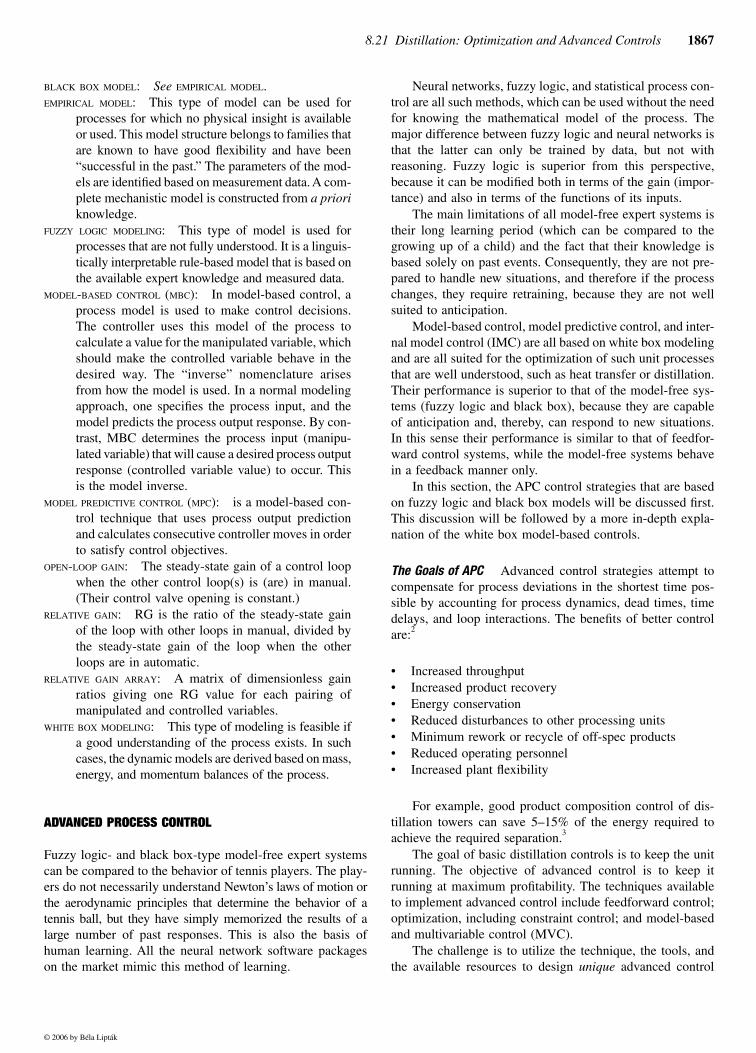
BLACK BOX MODEL: See EMPIRICAL MODEL.EMPIRICAL MODEL: This type of model can be used for
processes for which no physical insight is availableor used. This model structure belongs to families thatare known to have good flexibility and have been“successful in the past.” The parameters of the mod-els are identified based on measurement data. A com-plete mechanistic model is constructed from a prioriknowledge.
FUZZY LOGIC MODELING: This type of model is used forprocesses that are not fully understood. It is a linguis-tically interpretable rule-based model that is based onthe available expert knowledge and measured data.
MODEL-BASED CONTROL (MBC): In model-based control, aprocess model is used to make control decisions.The controller uses this model of the process tocalculate a value for the manipulated variable, whichshould make the controlled variable behave in thedesired way. The “inverse” nomenclature arisesfrom how the model is used. In a normal modelingapproach, one specifies the process input, and themodel predicts the process output response. By con-trast, MBC determines the process input (manipu-lated variable) that will cause a desired process outputresponse (controlled variable value) to occur. Thisis the model inverse.
MODEL PREDICTIVE CONTROL (MPC): is a model-based con-trol technique that uses process output predictionand calculates consecutive controller moves in orderto satisfy control objectives.
OPEN-LOOP GAIN: The steady-state gain of a control loopwhen the other control loop(s) is (are) in manual.(Their control valve opening is constant.)
RELATIVE GAIN: RG is the ratio of the steady-state gainof the loop with other loops in manual, divided bythe steady-state gain of the loop when the otherloops are in automatic.
RELATIVE GAIN ARRAY: A matrix of dimensionless gainratios giving one RG value for each pairing ofmanipulated and controlled variables.
WHITE BOX MODELING: This type of modeling is feasible ifa good understanding of the process exists. In suchcases, the dynamic models are derived based on mass,energy, and momentum balances of the process.
ADVANCED PROCESS CONTROL
Fuzzy logic- and black box-type model-free expert systemscan be compared to the behavior of tennis players. The play-ers do not necessarily understand Newton’s laws of motion orthe aerodynamic principles that determine the behavior of atennis ball, but they have simply memorized the results of alarge number of past responses. This is also the basis ofhuman learning. All the neural network software packageson the market mimic this method of learning.
Neural networks, fuzzy logic, and statistical process con-trol are all such methods, which can be used without the needfor knowing the mathematical model of the process. Themajor difference between fuzzy logic and neural networks isthat the latter can only be trained by data, but not withreasoning. Fuzzy logic is superior from this perspective,because it can be modified both in terms of the gain (impor-tance) and also in terms of the functions of its inputs.
The main limitations of all model-free expert systems istheir long learning period (which can be compared to thegrowing up of a child) and the fact that their knowledge isbased solely on past events. Consequently, they are not pre-pared to handle new situations, and therefore if the processchanges, they require retraining, because they are not wellsuited to anticipation.
Model-based control, model predictive control, and inter-nal model control (IMC) are all based on white box modelingand are all suited for the optimization of such unit processesthat are well understood, such as heat transfer or distillation.Their performance is superior to that of the model-free sys-tems (fuzzy logic and black box), because they are capableof anticipation and, thereby, can respond to new situations.In this sense their performance is similar to that of feedfor-ward control systems, while the model-free systems behavein a feedback manner only.
In this section, the APC control strategies that are basedon fuzzy logic and black box models will be discussed first.This discussion will be followed by a more in-depth expla-nation of the white box model-based controls.
The Goals of APC Advanced control strategies attempt tocompensate for process deviations in the shortest time pos-sible by accounting for process dynamics, dead times, timedelays, and loop interactions. The benefits of better controlare:2
• Increased throughput• Increased product recovery• Energy conservation• Reduced disturbances to other processing units• Minimum rework or recycle of off-spec products• Reduced operating personnel• Increased plant flexibility
For example, good product composition control of dis-tillation towers can save 5–15% of the energy required toachieve the required separation.3
The goal of basic distillation controls is to keep the unitrunning. The objective of advanced control is to keep itrunning at maximum profitability. The techniques availableto implement advanced control include feedforward control;optimization, including constraint control; and model-basedand multivariable control (MVC).
The challenge is to utilize the technique, the tools, andthe available resources to design unique advanced control
© 2006 by Béla Lipták
1868 Control and Optimization of Unit Operations
strategies that will match the specific objectives for the dis-tillation columns. The choice between any of these controltechniques depends upon factors such as preference and famil-iarity, complexity of scheme, degree of optimization, hard-ware for application, and number of variables monitored andcontrolled by single strategy.
Often, additional instrumentation is not needed whenimplementing advanced controls by building upon basic con-trol designs. However, in many cases, new measurements areneeded for calculation or compensation in order to implementan advanced control strategy. These must be retrofitted to theprocess.
Unlike basic distillation control, in which much of the con-trol can be implemented by analog control systems, advancedcontrol strategies usually require the use of higher-level com-puting systems. Optimization programs and model-basedcontrols require large amounts of computing power. It is forthis reason that APC control systems can be distributed overa variety of control equipment types in some kind of hierar-chical or distributed fashion.
Model-Based Control
The strategies presented in Sections 8.19 and 8.20 implementdistillation control using PID controllers. Efforts have beenmade to improve PID performance by considering the dynamicnature of the fractionator, the nonlinearity of the system, andthe decoupling of interactions.
Model-based controls have been gaining increasing pop-ularity and have been discussed in detail in Sections 2.13 to2.18 in Chapter 2. These use alternatives to the PID algorithmssuch as the internal model controller,12 model algorithmic con-trol,13 dynamic matrix control,14 and neural controllers.15 Pro-cess model-based control uses an approximate process modeldirectly for control in order to overcome the coupling effectsin the distillation tower.
Most of these methods are nonlinear, all are predictive,and many are multiple–input multiple-output (MIMO). Alldepend upon the availability of some process model. Once aprocess model has been established, it is possible to buildthe inverse of that model, which can be used as a controller.In that sense, the PID controller is a linear inverse model ofa single loop.
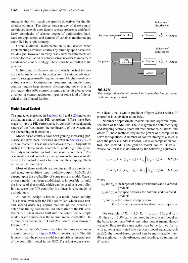
All control design is basically a model-based activity.This is true even with the PID controller, which uses first-and second-order lag approximations of the process todetermine tuning parameters. An alternative to the PID con-troller is a linear model built into the controller. A simplemodel-based controller is the internal model controller. Thedifference between the PID and IMC controller is shown inFigure 8.21a.
Note that the IMC looks like it has the same structure asa Smith predictor in Figure 8.19x in Section 8.19. The dif-ference is that the process model is explicitly an internal partof the controller model in the IMC. For a first-order system
with dead time, a Smith predictor (Figure 8.19x) with a PIcontroller is equivalent to an IMC.
Nonlinear approximate models include algebraic repre-sentation of the McCabe-Theile diagram for both rectifyingand stripping sections, short-cut fractionator calculations, andothers.16 These methods require the power of a computer tosolve the equations. A number of control strategies also existonce the process model is known. For dual composition con-trol, one method is the generic model control (GMC),17
whose control law is described by the following equations:
8.21(1)
8.21(2)
wherexsp and ysp = the target set points for bottoms and overhead
productsxss and yss = the specifications for bottoms and overhead
productsxo and yo = the current compositions
K = tunable parameters for disturbance rejection
For example, if K1,2 = 2.5, K2,2 = 0, xsp = 2%, and xo =1%, then xss = 3.5%. xss is then used in the process model asthe basis to compute V/B or any other output (manipulated)variable. Because the same action can be performed for yss
with yss being substituted into a process model equation, suchas D/L, the model-based control can be multivariable, han-dling nonlinearity, disturbances, and coupling, by tuning theK values.
FIG. 8.21aThe configuration of a PID control loop (top) and an internal modelcontroller loop (bottom).
Set point
Set point
Influence ofdisturbances
Controller
IMCcontroller
Process
Process
Model
Output
Output
Influence ofdisturbances
y y K y y K y y dto o oss sp sp= + − + −∫11 2 1, ,( ) ( )
x x K x x K x x dto o oss sp sp= + − + −∫1 2 2 2, ,( ) ( )
© 2006 by Béla Lipták
8.21 Distillation: Optimization and Advanced Controls 1869
Multivariable Control
Multivariable control is a technique that services multiple-input, multiple-output algorithms simultaneously as opposedto the single-input, single-output ones. MVC is particularlywell suited for highly interactive multivariable fractionators,where several control loops need to be decoupled. In general,the more difficult the process, the greater are the benefits ofmultivariable control. Multivariable control techniques cantake safety constraints, process lags, and economic optimi-zation factors all into consideration.
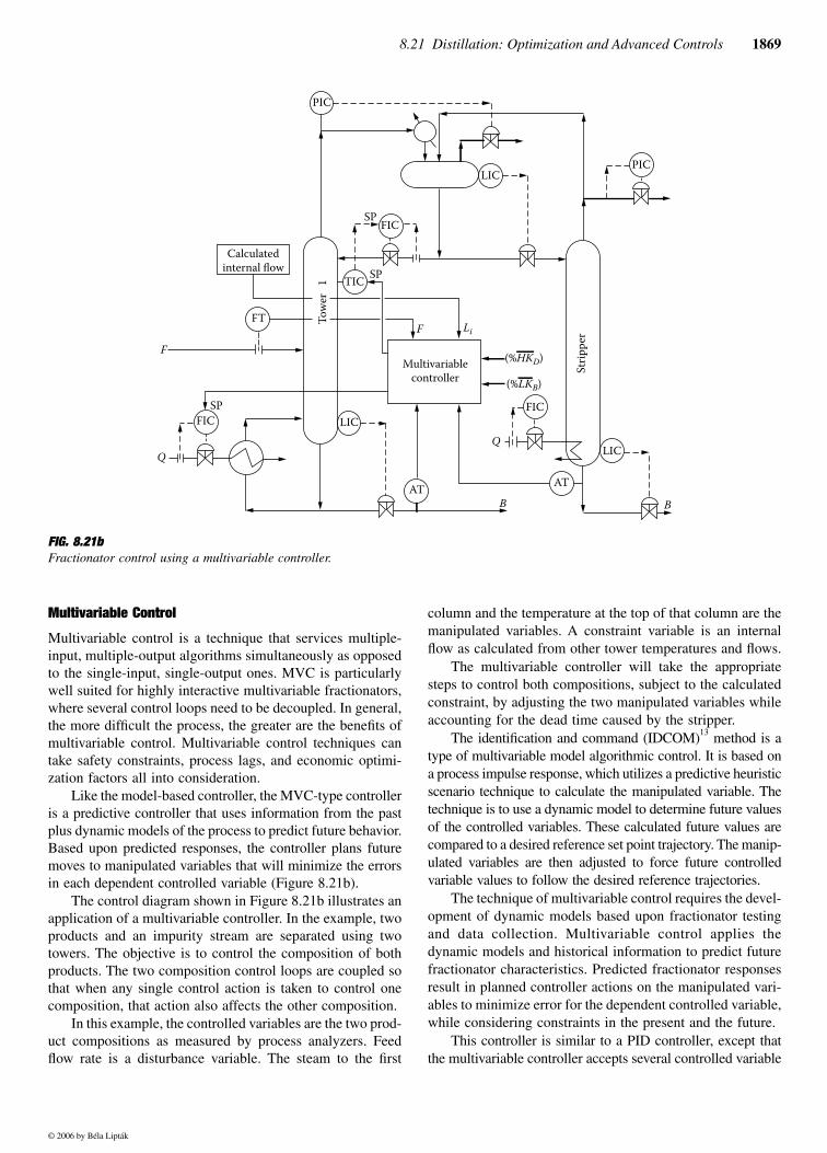
Like the model-based controller, the MVC-type controlleris a predictive controller that uses information from the pastplus dynamic models of the process to predict future behavior.Based upon predicted responses, the controller plans futuremoves to manipulated variables that will minimize the errorsin each dependent controlled variable (Figure 8.21b).
The control diagram shown in Figure 8.21b illustrates anapplication of a multivariable controller. In the example, twoproducts and an impurity stream are separated using twotowers. The objective is to control the composition of bothproducts. The two composition control loops are coupled sothat when any single control action is taken to control onecomposition, that action also affects the other composition.
In this example, the controlled variables are the two prod-uct compositions as measured by process analyzers. Feedflow rate is a disturbance variable. The steam to the first
column and the temperature at the top of that column are themanipulated variables. A constraint variable is an internalflow as calculated from other tower temperatures and flows.
The multivariable controller will take the appropriatesteps to control both compositions, subject to the calculatedconstraint, by adjusting the two manipulated variables whileaccounting for the dead time caused by the stripper.
The identification and command (IDCOM)13 method is atype of multivariable model algorithmic control. It is based ona process impulse response, which utilizes a predictive heuristicscenario technique to calculate the manipulated variable. Thetechnique is to use a dynamic model to determine future valuesof the controlled variables. These calculated future values arecompared to a desired reference set point trajectory. The manip-ulated variables are then adjusted to force future controlledvariable values to follow the desired reference trajectories.
The technique of multivariable control requires the devel-opment of dynamic models based upon fractionator testingand data collection. Multivariable control applies thedynamic models and historical information to predict futurefractionator characteristics. Predicted fractionator responsesresult in planned controller actions on the manipulated vari-ables to minimize error for the dependent controlled variable,while considering constraints in the present and the future.
This controller is similar to a PID controller, except thatthe multivariable controller accepts several controlled variable
FIG. 8.21bFractionator control using a multivariable controller.
AT
LICFICSP
Q
F
FT
Calculatedinternal flow
Multivariablecontroller
SP
LICPIC
PIC
SP
F
B
Q
FIC
(%HKD)
B
AT
LIC
Li
FIC
TIC
(%LKB)
Tow
er
Strip
per
1
© 2006 by Béla Lipták
1870 Control and Optimization of Unit Operations
set points and load variable measurements and, subject toconstraints, outputs several manipulated variables.
All multivariable techniques require some sort of processmodel. Differences between various multivariable techniqueslie in their calculation of internal models (whether nonlinearor linear), their method of predicting the future, their methodof constraint handling, and their method for minimizing thecontroller’s error.
Multivariable control may be considered to be an “over-kill” and at worst a poor controller, if simpler techniques areadequate. However, for towers that are subject to constraints,towers that have severe interactions, and towers with complexconfigurations, multivariable control can be a valuable tool.
Dynamic Matrix Control
A multivariable predictive controller is based on dynamicmatrix control.14 DMC is a predictive control technique thatuses a set of linear differential equations to describe theprocess. The DMC method is based upon a process stepresponse and calculates manipulated variable moves via aninverse model. Coefficients for the linear equations describingthe process dynamics are determined by process testing. Aseries of tests are conducted whereby a manipulated or loadvariable is perturbed and the dynamic response of all con-trolled variables is observed. This identification procedure istime-consuming and requires local expertise because of theexperimentation involved. Once the models are obtained, thecontroller design can be designed.
The least-squares approach is taken to minimize the errorof the controlled variables from their set points. Weightingconstants scale controlled variable errors and influence whichcontrolled variables are allowed to deviate from their setpoints if a constraint is encountered. The controller considersconstraints in its plan for both present and future moves ineach manipulated variable. Other factors affecting theresponse of the DMC controller are parameters that governthe relative amount of movement in the manipulated variablesand the rate at which errors are reduced. This is analogousto the tuning parameters in a PID controller.
Artificial Neural Networks
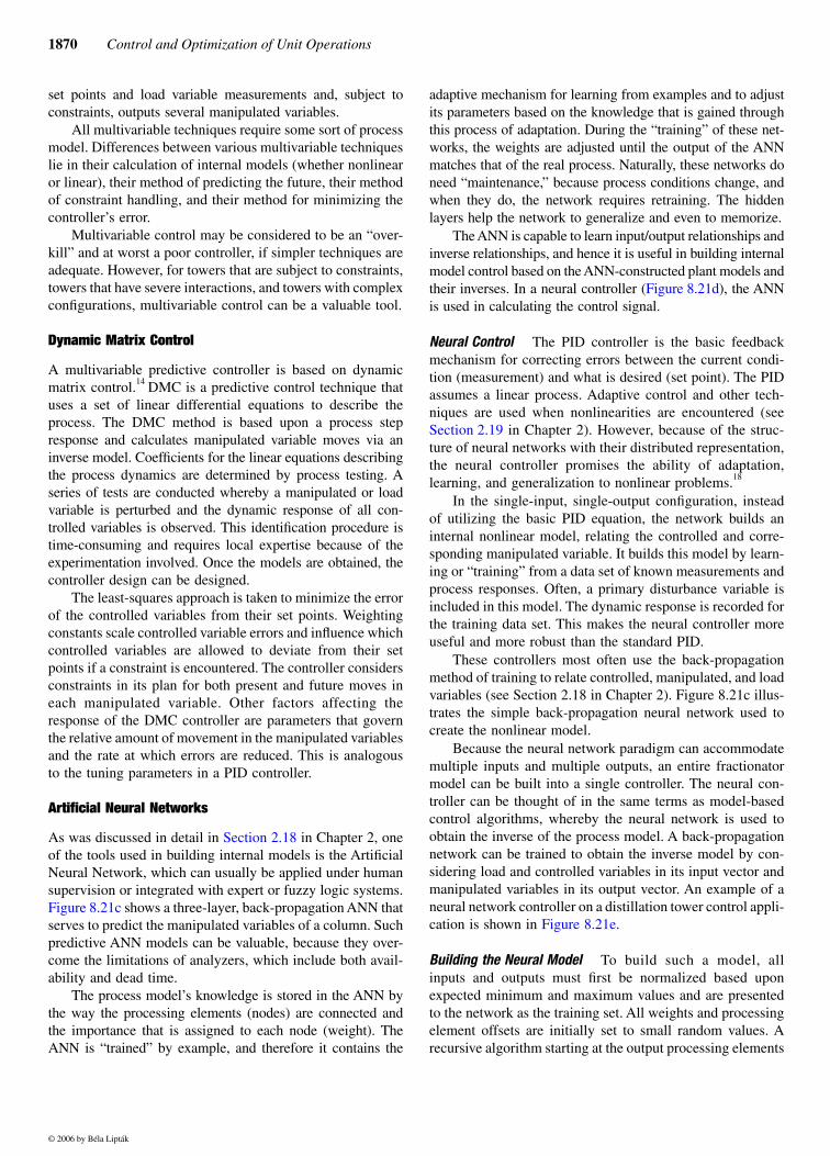
As was discussed in detail in Section 2.18 in Chapter 2, oneof the tools used in building internal models is the ArtificialNeural Network, which can usually be applied under humansupervision or integrated with expert or fuzzy logic systems.Figure 8.21c shows a three-layer, back-propagation ANN thatserves to predict the manipulated variables of a column. Suchpredictive ANN models can be valuable, because they over-come the limitations of analyzers, which include both avail-ability and dead time.
The process model’s knowledge is stored in the ANN bythe way the processing elements (nodes) are connected andthe importance that is assigned to each node (weight). TheANN is “trained” by example, and therefore it contains the
adaptive mechanism for learning from examples and to adjustits parameters based on the knowledge that is gained throughthis process of adaptation. During the “training” of these net-works, the weights are adjusted until the output of the ANNmatches that of the real process. Naturally, these networks doneed “maintenance,” because process conditions change, andwhen they do, the network requires retraining. The hiddenlayers help the network to generalize and even to memorize.
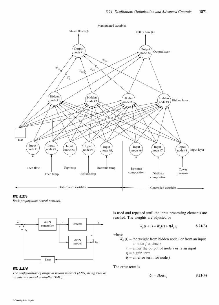
The ANN is capable to learn input/output relationships andinverse relationships, and hence it is useful in building internalmodel control based on the ANN-constructed plant models andtheir inverses. In a neural controller (Figure 8.21d), the ANNis used in calculating the control signal.
Neural Control The PID controller is the basic feedbackmechanism for correcting errors between the current condi-tion (measurement) and what is desired (set point). The PIDassumes a linear process. Adaptive control and other tech-niques are used when nonlinearities are encountered (seeSection 2.19 in Chapter 2). However, because of the struc-ture of neural networks with their distributed representation,the neural controller promises the ability of adaptation,learning, and generalization to nonlinear problems.18
In the single-input, single-output configuration, insteadof utilizing the basic PID equation, the network builds aninternal nonlinear model, relating the controlled and corre-sponding manipulated variable. It builds this model by learn-ing or “training” from a data set of known measurements andprocess responses. Often, a primary disturbance variable isincluded in this model. The dynamic response is recorded forthe training data set. This makes the neural controller moreuseful and more robust than the standard PID.
These controllers most often use the back-propagationmethod of training to relate controlled, manipulated, and loadvariables (see Section 2.18 in Chapter 2). Figure 8.21c illus-trates the simple back-propagation neural network used tocreate the nonlinear model.
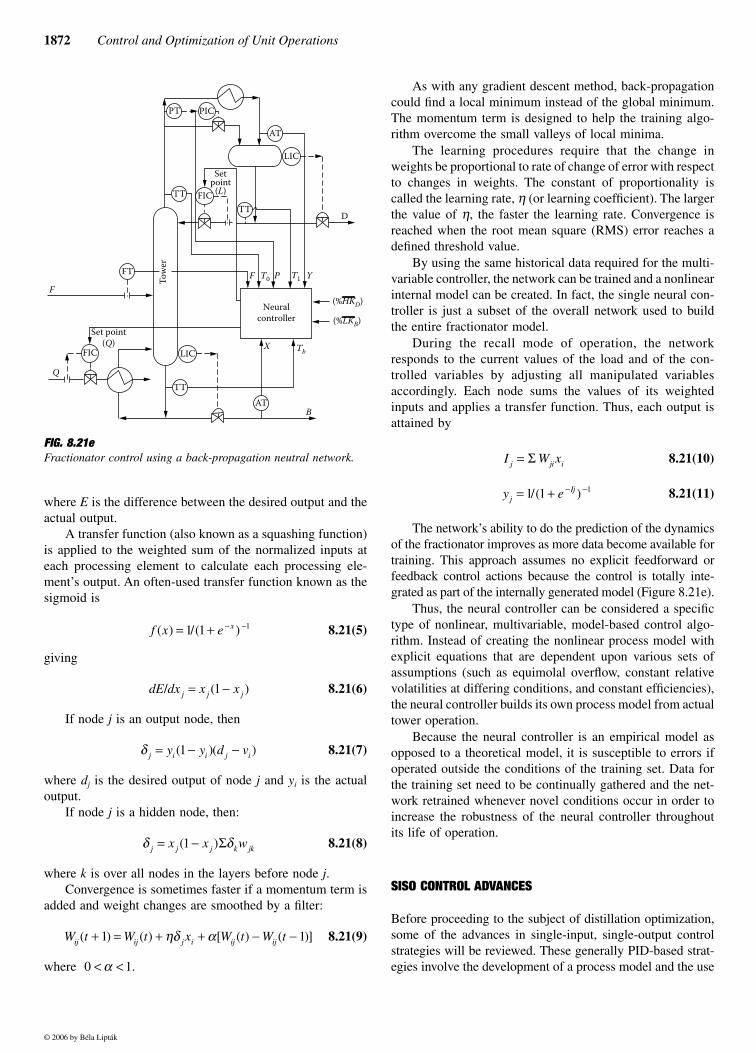
Because the neural network paradigm can accommodatemultiple inputs and multiple outputs, an entire fractionatormodel can be built into a single controller. The neural con-troller can be thought of in the same terms as model-basedcontrol algorithms, whereby the neural network is used toobtain the inverse of the process model. A back-propagationnetwork can be trained to obtain the inverse model by con-sidering load and controlled variables in its input vector andmanipulated variables in its output vector. An example of aneural network controller on a distillation tower control appli-cation is shown in Figure 8.21e.
Building the Neural Model To build such a model, allinputs and outputs must first be normalized based uponexpected minimum and maximum values and are presentedto the network as the training set. All weights and processingelement offsets are initially set to small random values. Arecursive algorithm starting at the output processing elements
© 2006 by Béla Lipták
8.21 Distillation: Optimization and Advanced Controls 1871
is used and repeated until the input processing elements arereached. The weights are adjusted by
8.21(3)
whereWij (t) = the weight from hidden node i or from an input
to node j at time txi = either the output of node i or is an inputη = a gain termδj = an error term for node j
The error term is
8.21(4)
FIG. 8.21cBack-propagation neural network.
Outputnode #1
Hiddennode #1
Inputnode #1
Inputnode #2
Inputnode #3
Inputnode #4
Inputnode #5
Inputnode #6
Inputnode #7
Inputnode #8 Input layer
Hiddennode #2
Hiddennode #3
Hiddennode #4 Hidden layer
Outputnode #2 Output layer
Manipulated variables
Steam flow (Q) Reflux flow (L)
Wj,0
Wj,1
Wj,2Wj,3
Wj,4
Bias
Feed flow
Feed temp
Top temp
Reflux temp
Disturbance variables Controlled variables
Bottoms temp Bottomscomposition Distillate
composition
Towerpressure
FIG. 8.21d The configuration of artificial neural network (ANN) being used asan internal model controller (IMC).
ANNcontroller
w u y
em
Process
ANNmodel
+−
+
−
ef
filter
W t W t xij ij j i( ) ( )+ = +1 ηδ
δ j jdE dx= /
© 2006 by Béla Lipták
1872 Control and Optimization of Unit Operations
where E is the difference between the desired output and theactual output.
A transfer function (also known as a squashing function)is applied to the weighted sum of the normalized inputs ateach processing element to calculate each processing ele-ment’s output. An often-used transfer function known as thesigmoid is
8.21(5)
giving
8.21(6)
If node j is an output node, then
8.21(7)
where dj is the desired output of node j and yi is the actualoutput.
If node j is a hidden node, then:
8.21(8)
where k is over all nodes in the layers before node j.Convergence is sometimes faster if a momentum term is
added and weight changes are smoothed by a filter:
8.21(9)
where
As with any gradient descent method, back-propagationcould find a local minimum instead of the global minimum.The momentum term is designed to help the training algo-rithm overcome the small valleys of local minima.
The learning procedures require that the change inweights be proportional to rate of change of error with respectto changes in weights. The constant of proportionality iscalled the learning rate, η (or learning coefficient). The largerthe value of η, the faster the learning rate. Convergence isreached when the root mean square (RMS) error reaches adefined threshold value.
By using the same historical data required for the multi-variable controller, the network can be trained and a nonlinearinternal model can be created. In fact, the single neural con-troller is just a subset of the overall network used to buildthe entire fractionator model.
During the recall mode of operation, the networkresponds to the current values of the load and of the con-trolled variables by adjusting all manipulated variablesaccordingly. Each node sums the values of its weightedinputs and applies a transfer function. Thus, each output isattained by
8.21(10)
8.21(11)
The network’s ability to do the prediction of the dynamicsof the fractionator improves as more data become available fortraining. This approach assumes no explicit feedforward orfeedback control actions because the control is totally inte-grated as part of the internally generated model (Figure 8.21e).
Thus, the neural controller can be considered a specifictype of nonlinear, multivariable, model-based control algo-rithm. Instead of creating the nonlinear process model withexplicit equations that are dependent upon various sets ofassumptions (such as equimolal overflow, constant relativevolatilities at differing conditions, and constant efficiencies),the neural controller builds its own process model from actualtower operation.
Because the neural controller is an empirical model asopposed to a theoretical model, it is susceptible to errors ifoperated outside the conditions of the training set. Data forthe training set need to be continually gathered and the net-work retrained whenever novel conditions occur in order toincrease the robustness of the neural controller throughoutits life of operation.
SISO CONTROL ADVANCES
Before proceeding to the subject of distillation optimization,some of the advances in single-input, single-output controlstrategies will be reviewed. These generally PID-based strat-egies involve the development of a process model and the use
FIG. 8.21eFractionator control using a back-propagation neutral network.
PT
TTTT
LIC
FIC
AT
PIC
FT
Set point(Q)
AT
LIC
TTQ
FIC
F
Neuralcontroller
(%HKD)
(%LKB)
X
D
F P Y
B
Tb
T1T0
Setpoint
(L)
Tow
er
f x e x( ) /( )= + − −1 1 1
dE dx x xj j j/ ( )= −1
δ j i i j iy y d v= − −( )( )1
δ δj j j k jkx x w= −( )1 Σ
W t W t x W t W tij ij j i ij ij( ) ( ) [ ( ) ( )]+ = + + − −1 1ηδ α
0 1< <α .
I W xj ji i= Σ
y ejIj= + − −1 1 1/( )
© 2006 by Béla Lipták
8.21 Distillation: Optimization and Advanced Controls 1873
of feedforward and supervisory control techniques to achievebetter control quality and localized optimization goals.
Process Model
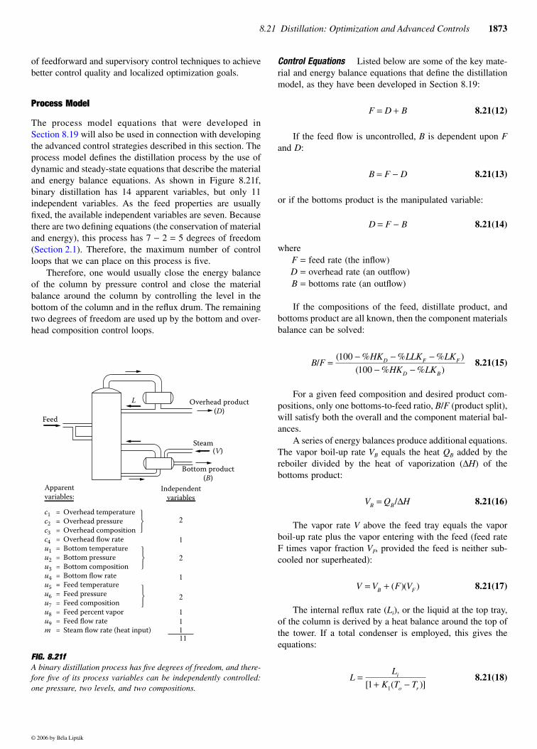
The process model equations that were developed inSection 8.19 will also be used in connection with developingthe advanced control strategies described in this section. Theprocess model defines the distillation process by the use ofdynamic and steady-state equations that describe the materialand energy balance equations. As shown in Figure 8.21f,binary distillation has 14 apparent variables, but only 11independent variables. As the feed properties are usuallyfixed, the available independent variables are seven. Becausethere are two defining equations (the conservation of materialand energy), this process has 7 − 2 = 5 degrees of freedom(Section 2.1). Therefore, the maximum number of controlloops that we can place on this process is five.
Therefore, one would usually close the energy balanceof the column by pressure control and close the materialbalance around the column by controlling the level in thebottom of the column and in the reflux drum. The remainingtwo degrees of freedom are used up by the bottom and over-head composition control loops.
Control Equations Listed below are some of the key mate-rial and energy balance equations that define the distillationmodel, as they have been developed in Section 8.19:
8.21(12)
If the feed flow is uncontrolled, B is dependent upon Fand D:
8.21(13)
or if the bottoms product is the manipulated variable:
8.21(14)
whereF = feed rate (the inflow)D = overhead rate (an outflow)B = bottoms rate (an outflow)
If the compositions of the feed, distillate product, andbottoms product are all known, then the component materialsbalance can be solved:
8.21(15)
For a given feed composition and desired product com-positions, only one bottoms-to-feed ratio, B/F (product split),will satisfy both the overall and the component material bal-ances.
A series of energy balances produce additional equations.The vapor boil-up rate VB equals the heat QB added by thereboiler divided by the heat of vaporization (∆H) of thebottoms product:
8.21(16)
The vapor rate V above the feed tray equals the vaporboil-up rate plus the vapor entering with the feed (feed rateF times vapor fraction VF, provided the feed is neither sub-cooled nor superheated):
8.21(17)
The internal reflux rate (Li), or the liquid at the top tray,of the column is derived by a heat balance around the top ofthe tower. If a total condenser is employed, this gives theequations:
8.21(18)
FIG. 8.21fA binary distillation process has five degrees of freedom, and there-fore five of its process variables can be independently controlled:one pressure, two levels, and two compositions.
c1 = Overhead temperaturec2 = Overhead pressurec3 = Overhead compositionc4 = Overhead flow rateu1 = Bottom temperatureu2 = Bottom pressureu3 = Bottom compositionu4 = Bottom flow rateu5 = Feed temperatureu6 = Feed pressureu7 = Feed compositionu8 = Feed percent vaporu9 = Feed flow ratem = Steam flow rate (heat input)
2
2
1
1
111
2
11
Apparentvariables:
Independentvariables
Feed
L Overhead product(D)
Bottom product(B)
Steam(V)
F D B= +
B F D= −
D F B= −
B FHK LLK LK
HK LKD F F
D B
/( % % % )
( % % )=
− − −− −
100
100
V Q HB B= /∆
V V F VB F= + ( )( )
LL
K T Ti
o r
=+ −[ ( )]1 1
© 2006 by Béla Lipták
1874 Control and Optimization of Unit Operations
or
8.21(19)
The liquid rate, Lf, below the feed tray equals the internalreflux plus the liquid in the feed:
8.21(20)
The distillate rate, D, equals the vapor rate, V, minus theinternal reflux:
8.21(21)
The bottoms rate, B, equals the liquid rate, Lf, minus the boil-up, VB:
8.21(22)
The criterion for separation is the ratio of reflux (L) to distil-late (D) vs. the ratio of boil-up (V) to bottoms (B). Manipu-lating reflux affects separation equally as well as manipulat-ing boil-up, albeit in opposite directions. Thus, for a two-product tower, two equations define the process: One is anequation describing separation and the other is an equationfor material balance.
During the unsteady state of upsets, the process modelmust account for the dynamics of the process. This extendsthe steady-state internal flow model and requires additionalconsideration. For this reason two dynamic terms, GT andGB, are included, which provides a dynamic model for thetower based on its dead time and second-order lag, giving
8.21 (23)
where
whereta, tb = dead times
Scaling When using process models, it is very importantthat the measurements be correctly represented, that all I/Ovalues be properly scaled. This was less of a challenge in theanalog age, when a 9 PSIG or a 12 mA signal always meant50%, no matter which supplier, industry, or continent wasinvolved. This is not necessarily the case in the present digitalage, with its multiple protocols and the need for interfacingtranslators when connecting them.
Scaling (the conversion from engineering units to frac-tions or percentages) is required in order to make the varioustransmitter signals meaningful to the DCS, PLC, or other
central control system. A simple example of this type of con-version has already been given for zero-based signals in con-nection with Figure 8.19l in Section 8.19. In this sectionscaling will be illustrated on more complex systems, involvingseveral nonzero-based transmitter signals.
The value of a transmitted signal in engineering units canbe obtained from the normalized (scaled) transmitter signaland from the zero and range of the transmitter as follows:
8.21(24)
Inversely, the percentage transmitter signal (scaled equiv-alent) corresponding to an engineering measurement can beobtained as
8.21(25)
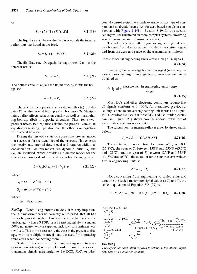
Most DCS and other electronic controllers require thatall signals conform to 0–100%. As mentioned previously,scaling is done to convert engineering unit inputs and outputsinto normalized values that these DCS and electronic systemscan use. Figure 8.21g shows how the internal reflux rate ofa distillation column is calculated.
The calculation for internal reflux is given by the equationbelow:
LI = L.[1 + (CP/∆H)∆T ] 8.21(26)
The subtracter is scaled first. Assuming ∆Tmax of 50°F(27.8°C), the span of To between 150°F and 250°F (65.6°Cand 121°C), and the span of Tr between 125°F and 225°F(51.7°C and 107°C), the equation for the subtracter is writtenfirst in engineering units as
8.21(27)
Now, converting from engineering to scaled units anddenoting the scaled transmitter signal values as and thescaled equivalent of Equation 8.21(27) is
8.21(28)
L L K Ti r= ⋅ +( ) [ ( )( )]1 ∆
L L V Ff i F= + −( )( )1
D V Li= −
B L Vf B= −
L G G L V FB T i F= + − ⋅[ ( ) ]1
G ta e e
G tb e e
Bt t
Tt t
= − −
= − −
− −
− −
( )( )
( )( )
1 1
1 1
1 2
3 4
FIG. 8.21gThe steps in the calculation required to determine the internal refluxflow rate of a distillation column.
measurement in engineering units zero range= + signal(% )
% signalmeasurement in engineering units ze= − rro
range
∆T T To r= −
′To ′Tr ,
0 50 150 100 125 100+ ′ = + ′ − + ′∆T T To r( ) ( )
150−250°F = 0−100%To
125−225°F = 0−100%Tr To−Tr
L
X
L2
TT
TT
FT FY
TY UY
0−10,000 GPM 0−50°F = 0−100%
∆ Li = L (1 + CP∆H
∆T)
[Li′ = 0.754 L′ (0.885+ 0.115∆T′)]
© 2006 by Béla Lipták
8.21 Distillation: Optimization and Advanced Controls 1875
This reduces to the scaled equations:
8.21(29)
If the following assumptions are made:
LI max = 15,000 gpm (0.95 m3/s)Lmax = 10,000 gpm (0.63 m3/s)Cp = 0.65 BTU/lb°F (0.65 kcal/kg°C)∆H = 250 BTU/lb (450 kcal/kg)
the equation for the multiplier then becomes
8.21(30)
Equation 8.21(30) then reduces to
8.21(31)
When ∆T ′ is zero, the internal reflux equals 0.667 timesthe external reflux. The number 1 within the parentheses,therefore, sets the minimum internal reflux. When is100%, the ratio of internal reflux to external reflux is at amaximum.
The expression within the parentheses must be normalized.This is done by dividing both terms by the total numericalvalue, that is 1.13. To preserve the equality, the coefficientof is multiplied by 1.13. The scaled equation becomes
8.21(32)
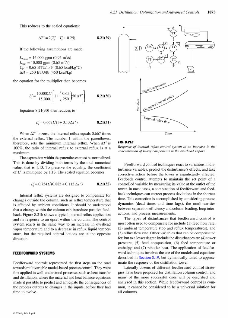
Internal reflux systems are designed to compensate forchanges outside the column, such as reflux temperature thatis affected by ambient conditions. It should be understoodthat a change within the column can introduce positive feed-back. Figure 8.21h shows a typical internal reflux applicationand its response to an upset within the column. The controlsystem reacts in the same way to an increase in overheadvapor temperature and to a decrease in reflux liquid temper-ature, but the required control actions are in the oppositedirection.
FEEDFORWARD SYSTEMS
Feedforward controls represented the first steps on the roadtowards multivariable model-based process control. They werefirst applied in well-understood processes such as heat transferand distillation, where the material and heat balance equationsmade it possible to predict and anticipate the consequences ofthe process outputs to changes in the inputs, before they hadtime to evolve.
Feedforward control techniques react to variations in dis-turbance variables, predict the disturbance’s effects, and takecorrective action before the tower is significantly affected.Feedback control attempts to maintain the set point of acontrolled variable by measuring its value at the outlet of thetower. In most cases, a combination of feedforward and feed-back techniques can correct process deviations in the shortesttime. This correction is accomplished by considering processdynamics (dead times and time lags), the nonlinearitiesbetween separation efficiency and column loading, loop inter-actions, and process measurements.
The types of disturbances that feedforward control ismost often used to compensate for include (1) feed flow rate,(2) ambient temperature (top and reflux temperatures), and(3) reflux flow rate. Other variables that can be compensatedfor, but to a lesser degree include the disturbances are (4) towerpressure, (5) feed composition, (6) feed temperature orenthalpy, and (7) reboiler heat. The application of feedfor-ward techniques involves the use of the models and equationsdescribed in Section 8.19, but dynamically tuned to approx-imate the response of the distillation tower.
Literally dozens of different feedforward control strate-gies have been proposed for distillation column control, andmany of the more successful ones will be described andanalyzed in this section. While feedforward control is com-mon, it cannot be considered to be a universal solution forall columns.
∆ ′ = ′ − ′ +T T To r2 0 25( . )
′ = ′ +
′
L
LTi
10 00015 000
10 65250
50,,
. ∆
′ = ′ + ′L L Ti 0 667 1 0 13. ( . )∆
∆ ′T
′L
′ = ′ + ′L L Ti 0 754 0 885 0 115. ( . . )∆
FIG. 8.21hResponse of internal reflux control system to an increase in theconcentration of heavy components in the overhead vapors.
FRCX ∆
TY
TT
UY
FT
To
FY TTTr
Varia
bles
Vapor temperature
Computed internal reflux
External reflux flow
Time
© 2006 by Béla Lipták
1876 Control and Optimization of Unit Operations
Flow Control of Distillate
The column interactions that otherwise might necessitate theuse of an internal reflux control system can be eliminated insome cases when the flow of distillate product draw-off iscontrolled and reflux is put under accumulator level control.This is a slower system than one in which flow controls thereflux, and its response is not always adequate. If necessary,the response can be speeded up by reduction of the accumu-lator lag.4
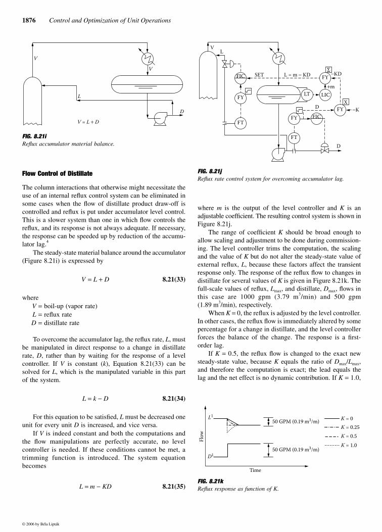
The steady-state material balance around the accumulator(Figure 8.21i) is expressed by
8.21(33)
whereV = boil-up (vapor rate)L = reflux rateD = distillate rate
To overcome the accumulator lag, the reflux rate, L, mustbe manipulated in direct response to a change in distillaterate, D, rather than by waiting for the response of a levelcontroller. If V is constant (k), Equation 8.21(33) can besolved for L, which is the manipulated variable in this partof the system.
8.21(34)
For this equation to be satisfied, L must be decreased oneunit for every unit D is increased, and vice versa.
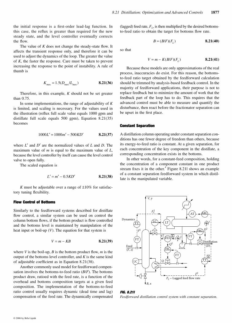
If V is indeed constant and both the computations andthe flow manipulations are perfectly accurate, no levelcontroller is needed. If these conditions cannot be met, atrimming function is introduced. The system equationbecomes
8.21(35)
where m is the output of the level controller and K is anadjustable coefficient. The resulting control system is shown inFigure 8.21j.
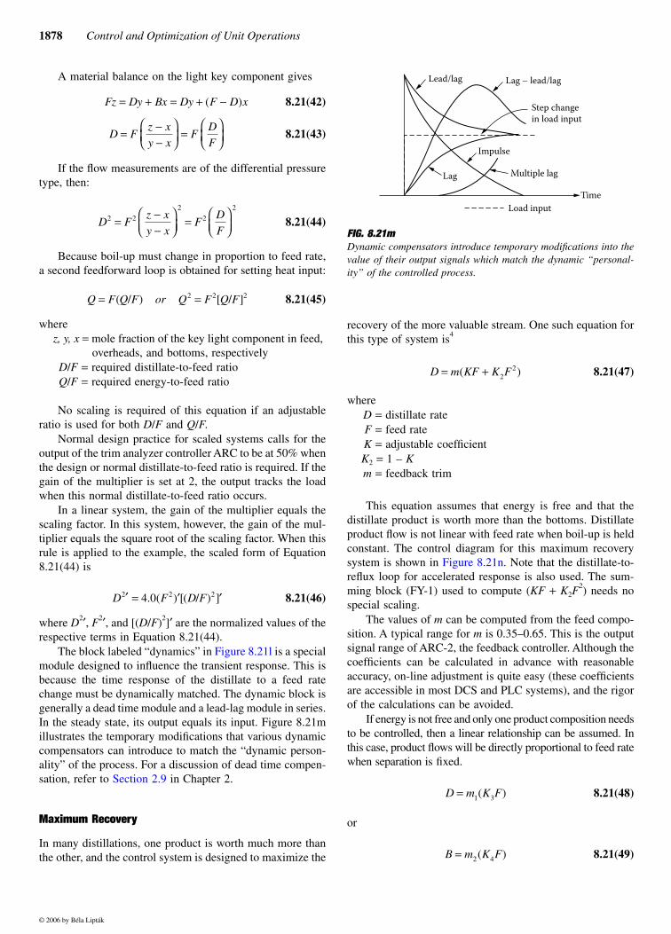
The range of coefficient K should be broad enough toallow scaling and adjustment to be done during commission-ing. The level controller trims the computation, the scalingand the value of K but do not alter the steady-state value ofexternal reflux, L, because these factors affect the transientresponse only. The response of the reflux flow to changes indistillate for several values of K is given in Figure 8.21k. Thefull-scale values of reflux, Lmax, and distillate, Dmax, flows inthis case are 1000 gpm (3.79 m3/min) and 500 gpm(1.89 m3/min), respectively.
When K = 0, the reflux is adjusted by the level controller.In other cases, the reflux flow is immediately altered by somepercentage for a change in distillate, and the level controllerforces the balance of the change. The response is a first-order lag.
If K = 0.5, the reflux flow is changed to the exact newsteady-state value, because K equals the ratio of Dmax/Lmax,and therefore the computation is exact; the lead equals thelag and the net effect is no dynamic contribution. If K = 1.0,
FIG. 8.21i Reflux accumulator material balance.
V
L
V
D
V = L + D
V L D= +
L k D= −
L m KD= −
FIG. 8.21jReflux rate control system for overcoming accumulator lag.
FIG. 8.21kReflux response as function of K.
VL
FIC SET L = m − KD
FY
FTFIC
FY
LIC
FT
FYFY
LT
−KD
+m
Σ
XD
D
−K
50 GPM (0.19 m3/m)
50 GPM (0.19 m3/m)
Time
K = 0K = 0.25K = 0.5K = 1.0
Flow
L1
D1
© 2006 by Béla Lipták
8.21 Distillation: Optimization and Advanced Controls 1877
the initial response is a first-order lead-lag function. Inthis case, the reflux is greater than required for the newsteady state, and the level controller eventually correctsthe flow.
The value of K does not change the steady-state flow. Itaffects the transient response only, and therefore it can beused to adjust the dynamics of the loop. The greater the valueof K, the faster the response. Care must be taken to preventincreasing the response to the point of instability. A rule ofthumb is
8.21(36)
Therefore, in this example, K should not be set greaterthan 0.75.
In some implementations, the range of adjustability of Kis limited, and scaling is necessary. For the values used inthe illustration (reflux full scale value equals 1000 gpm anddistillate full scale equals 500 gpm), Equation 8.21(35)becomes
8.21(37)
where L′ and D′ are the normalized values of L and D. Themaximum value of m is equal to the maximum value of L,because the level controller by itself can cause the level controlvalve to open fully.
The scaled equation is
8.21(38)
K must be adjustable over a range of ±10% for satisfac-tory tuning flexibility.
Flow Control of Bottoms
Similarly to the feedforward systems described for distillateflow control, a similar system can be used on control thecolumn bottom flows, if the bottom product is flow controlledand the bottoms level is maintained by manipulation of theheat input or boil-up (V). The equation for that system is
8.21(39)
where V is the boil-up, B is the bottom product flow, m is theoutput of the bottoms level controller, and K is the same kindof adjustable coefficient as in Equation 8.21(38).
Another commonly used model for feedforward compen-sation involves the bottoms-to-feed ratio (B/F). The bottomsproduct draw, ratioed with the feed rate, is a function of theoverhead and bottoms composition targets at a given feedcomposition. The implementation of the bottoms-to-feedratio control usually requires dynamic (dead time and lag)compensation of the feed rate. The dynamically compensated
(lagged) feed rate, FL, is then multiplied by the desired bottoms-to-feed ratio to obtain the target for bottoms flow rate.
8.21(40)
so that
8.21(41)
Because these models are only approximations of the realprocess, inaccuracies do exist. For this reason, the bottoms-to-feed ratio target obtained by the feedforward calculationshould be trimmed by analysis-based feedback control. In themajority of feedforward applications, their purpose is not toreplace feedback but to minimize the amount of work that thefeedback part of the loop has to do. This requires that theadvanced control must be able to measure and quantify thedisturbance, then react before the fractionator separation canbe upset in the first place.
Constant Separation
A distillation column operating under constant separation con-ditions has one fewer degree of freedom than others, becauseits energy-to-feed ratio is constant. At a given separation, foreach concentration of the key component in the distillate, acorresponding concentration exists in the bottoms.
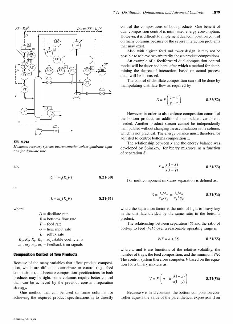
In other words, for a constant-feed composition, holdingthe concentration of a component constant in one productstream fixes it in the other.4 Figure 8.21l shows an exampleof a constant separation feedforward system in which distil-late is the manipulated variable.
K D Lmax max max. ( / )= 1 5
1000 1000 500′ = ′ − ′L m KD
′ = ′ − ′L m KD0 5.
V m KB= −
FIG. 8.21lFeedforward distillation control system with constant separation.
B B F FL= ( / )( )
V m K B F FL= − ( / )( )
DynamicsFY
FT
LC
AT
F
FTDistillation
(D)
D2
D
ARC
FRC
V, y
LF2
Q2
FL – Lagged feed flow rateF2
FL2
FL2
LT
FFY
FYX
FIC
QLC
Feed(F, z)
B, x
FT
X
( (2
FQ( (2
© 2006 by Béla Lipták
1878 Control and Optimization of Unit Operations
A material balance on the light key component gives
8.21(42)
8.21(43)
If the flow measurements are of the differential pressuretype, then:
8.21(44)
Because boil-up must change in proportion to feed rate,a second feedforward loop is obtained for setting heat input:
8.21(45)
wherez, y, x = mole fraction of the key light component in feed,
overheads, and bottoms, respectivelyD/F = required distillate-to-feed ratioQ/F = required energy-to-feed ratio
No scaling is required of this equation if an adjustableratio is used for both D/F and Q/F.
Normal design practice for scaled systems calls for theoutput of the trim analyzer controller ARC to be at 50% whenthe design or normal distillate-to-feed ratio is required. If thegain of the multiplier is set at 2, the output tracks the loadwhen this normal distillate-to-feed ratio occurs.
In a linear system, the gain of the multiplier equals thescaling factor. In this system, however, the gain of the mul-tiplier equals the square root of the scaling factor. When thisrule is applied to the example, the scaled form of Equation8.21(44) is
8.21(46)
where D2′, F2′, and [(D/F)2]′ are the normalized values of therespective terms in Equation 8.21(44).
The block labeled “dynamics” in Figure 8.21l is a specialmodule designed to influence the transient response. This isbecause the time response of the distillate to a feed ratechange must be dynamically matched. The dynamic block isgenerally a dead time module and a lead-lag module in series.In the steady state, its output equals its input. Figure 8.21millustrates the temporary modifications that various dynamiccompensators can introduce to match the “dynamic person-ality” of the process. For a discussion of dead time compen-sation, refer to Section 2.9 in Chapter 2.
Maximum Recovery
In many distillations, one product is worth much more thanthe other, and the control system is designed to maximize the
recovery of the more valuable stream. One such equation forthis type of system is4
8.21(47)
whereD = distillate rateF = feed rateK = adjustable coefficientK2 = 1 – K m = feedback trim
This equation assumes that energy is free and that thedistillate product is worth more than the bottoms. Distillateproduct flow is not linear with feed rate when boil-up is heldconstant. The control diagram for this maximum recoverysystem is shown in Figure 8.21n. Note that the distillate-to-reflux loop for accelerated response is also used. The sum-ming block (FY-1) used to compute (KF + K2F
2) needs nospecial scaling.
The values of m can be computed from the feed compo-sition. A typical range for m is 0.35–0.65. This is the outputsignal range of ARC-2, the feedback controller. Although thecoefficients can be calculated in advance with reasonableaccuracy, on-line adjustment is quite easy (these coefficientsare accessible in most DCS and PLC systems), and the rigorof the calculations can be avoided.
If energy is not free and only one product composition needsto be controlled, then a linear relationship can be assumed. Inthis case, product flows will be directly proportional to feed ratewhen separation is fixed.
8.21(48)
or
8.21(49)
Fz Dy Bx Dy F D x= + = + −( )
D Fz xy x
FDF
= −−
=
D Fz xy x
FDF
2 2
2
2
2
= −−
=
Q F Q F or Q F Q F= =( / ) [ / ]2 2 2
D F D F2 2 24 0′ = ′ ′. ( ) [( / ) ]
FIG. 8.21mDynamic compensators introduce temporary modifications into thevalue of their output signals which match the dynamic “personal-ity” of the controlled process.
Load input
Lag Multiple lag
Impulse
Time
Lag – lead/lagLead/lag
Step changein load input
D m KF K F= +( )22
D m K F= 1 3( )
B m K F= 2 4( )
© 2006 by Béla Lipták
8.21 Distillation: Optimization and Advanced Controls 1879
and
8.21(50)
or
8.21(51)
whereD = distillate rateB = bottoms flow rateF = feed rateQ = heat input rateL = reflux rate
K3, K4, K5, K6 = adjustable coefficientsm1, m2, m3, m4 = feedback trim signals
Composition Control of Two Products
Because of the many variables that affect product composi-tion, which are difficult to anticipate or control (e.g., feedcomposition), and because composition specifications for bothproducts may be tight, some columns require better controlthan can be achieved by the previous constant separationstrategy.
One method that can be used on some columns forachieving the required product specifications is to directly
control the compositions of both products. One benefit ofdual composition control is minimized energy consumption.However, it is difficult to implement dual composition controlon many columns because of the severe interaction problemsthat may exist.
Also, with a given feed and tower design, it may not bepossible to achieve two arbitrarily chosen product compositions.
An example of a feedforward dual-composition controlmodel will be described here, after which a method for deter-mining the degree of interaction, based on actual processdata, will be discussed.
The control of distillate composition can still be done bymanipulating distillate flow as required by
8.22(52)
However, in order to also enforce composition control ofthe bottom product, an additional manipulated variable isneeded. Another product stream cannot be independentlymanipulated without changing the accumulation in the column,which is not practical. The energy balance must, therefore, beadjusted to control bottoms composition x.
The relationship between x and the energy balance wasdeveloped by Shinskey,5 for binary mixtures, as a functionof separation S:
8.21(53)
For multicomponent mixtures separation is defined as:
8.21(54)
where the separation factor is the ratio of light to heavy keyin the distillate divided by the same ratio in the bottomsproduct.
The relationship between separation (S) and the ratio ofboil-up to feed (V/F) over a reasonable operating range is
8.21(55)
where a and b are functions of the relative volatility, thenumber of trays, the feed composition, and the minimum V/F.The control system therefore computes V based on the equa-tion for a binary mixture as
8.21(56)
Because y is held constant, the bottom composition con-troller adjusts the value of the parenthetical expression if an
FIG. 8.21nMaximum recovery system: instrumentation solves quadratic equa-tion for distillate rate.
X∆m
Σ2
D
FY
ARC
LIC
LT
FY
FICFY
FT
F
LCQ
B
FY FTAT
F V1
L
D
D = m (KF + K2F2)KF + K2F2
FT
FYSP
FRCF2
FY
Q m K F= 3 5( )
L m K F= 4 6( )
D Fz xy x
= −−
Sy xx y
= −−
( )( )11
Sy x
x y
y x
x yL L
H H
L H
L H
= =/
/
/
/
V F a bS/ = +
V F a by xx y
= + −−
( )( )11
© 2006 by Béla Lipták
1880 Control and Optimization of Unit Operations
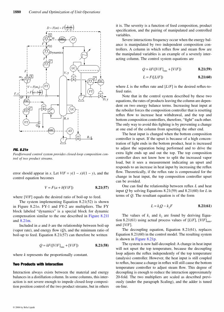
error should appear in x. Let V/F = y(1 − x)/(1 − y), and thecontrol equation becomes
8.21(57)
where [V/F] equals the desired ratio of boil-up to feed.The system implementing Equation 8.21(52) is shown
in Figure 8.21o. FY-1 and FY-2 are multipliers. The FYblock labeled “dynamics” is a special block for dynamiccompensation similar to the one described in Figure 8.21land 8.21m.
Included in a and b are the relationship between boil-up(vapor rate), and energy flow (Q), and the minimum ratio ofboil-up to feed. Equation 8.21(57) can therefore be written
8.21(58)
where k represents the proportionally constant.
Two Products with Interaction
Interaction always exists between the material and energybalances in a distillation column. In some columns, this inter-action is not severe enough to impede closed-loop composi-tion position control of the two product streams, but in others
it is. The severity is a function of feed composition, productspecification, and the pairing of manipulated and controlledvariables.
Severe interactions frequency occur when the energy bal-ance is manipulated by two independent composition con-trollers. A column in which reflux flow and steam flow arethe manipulated variables is an example of a severely inter-acting column. The control system equations are
8.21(59)
8.21(60)
where L is the reflux rate and [L/F] is the desired reflux-to-feed ratio.
Note that in the control system described by these twoequations, the rates of products leaving the column are depen-dent on two energy balance terms. Increasing heat input atthe reboiler forces the composition controller that is resettingreflux flow to increase heat withdrawal, and the top andbottom composition controllers, therefore, “fight” each other.The only way to avoid this fighting is by preventing a changeat one end of the column from upsetting the other end.
The heat input is changed when the bottom compositioncontroller is upset. If the upset is because of a high concen-tration of light ends in the bottom product, heat is increasedto adjust the separation being performed and to drive theextra light ends up and out the top. The top compositioncontroller does not know how to split the increased vaporload, but it sees a measurement indicating an upset andresponds to an increase in heat input by increasing the refluxflow. Theoretically, if the reflux rate is compensated for thechange in heat input, the top composition controller upsetcan be avoided.
One can find the relationship between reflux L and heatinput Q by solving Equations 8.21(59) and 8.21(60) for L interms of Q. The resultant equation is of the form
8.21(61)
The values of k1 and k2 are found by deriving Equa-tion 8.21(61) using actual process values of [L/F], [V/F]min,and [V/F].
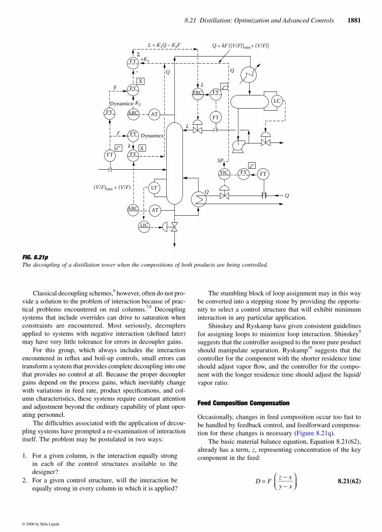
The decoupling equation, Equation 8.21(61), replacesEquation 8.21(60) in the control model. The resulting systemis shown in Figure 8.21p.
The system is now half-decoupled: A change in heat inputwill not upset the top temperature, because the decouplingloop adjusts the reflux independently of the top temperature(analysis) controller. However, the heat input is still coupledto reflux, because a change in reflux will still cause the bottomtemperature controller to adjust steam flow. This degree ofdecoupling is enough to reduce the interaction approximately20-fold. The two multipliers are scaled as described previ-ously (under the paragraph Scaling), and the adder is tunedon-line.
FIG. 8.21oFeedforward control system provides closed-loop composition con-trol of two product streams.
Xm
FF(t)
FY
FFY
Dynamics
LC
FT
F, zVF
m2 FY2V = F(m2) == F a+b
X
ARC ATFY
F
FY
FICVSP
QARC AT
LC
FY
FT
FIC
B, x
B, x
V, y
D, y
FT
D = F(m) = F z−xy−x
V F a b V F= +( [ / ])
Q kF V F V F= +([ / ] [ / ])min
Q kF V F V F= +([ / ] [ / ])min
L F L F= ([ / ])
L k Q k F= −1 2
© 2006 by Béla Lipták
8.21 Distillation: Optimization and Advanced Controls 1881
Classical decoupling schemes,6 however, often do not pro-vide a solution to the problem of interaction because of prac-tical problems encountered on real columns.7,8 Decouplingsystems that include overrides can drive to saturation whenconstraints are encountered. Most seriously, decouplersapplied to systems with negative interaction (defined later)may have very little tolerance for errors in decoupler gains.
For this group, which always includes the interactionencountered in reflux and boil-up controls, small errors cantransform a system that provides complete decoupling into onethat provides no control at all. Because the proper decouplergains depend on the process gains, which inevitably changewith variations in feed rate, product specifications, and col-umn characteristics, these systems require constant attentionand adjustment beyond the ordinary capability of plant oper-ating personnel.
The difficulties associated with the application of decou-pling systems have prompted a re-examination of interactionitself. The problem may be postulated in two ways:
1. For a given column, is the interaction equally strongin each of the control structures available to thedesigner?
2. For a given control structure, will the interaction beequally strong in every column in which it is applied?
The stumbling block of loop assignment may in this waybe converted into a stepping stone by providing the opportu-nity to select a control structure that will exhibit minimuminteraction in any particular application.
Shinskey and Ryskamp have given consistent guidelinesfor assigning loops to minimize loop interaction. Shinskey9
suggests that the controller assigned to the more pure productshould manipulate separation. Ryskamp10 suggests that thecontroller for the component with the shorter residence timeshould adjust vapor flow, and the controller for the compo-nent with the longer residence time should adjust the liquid/vapor ratio.
Feed Composition Compensation
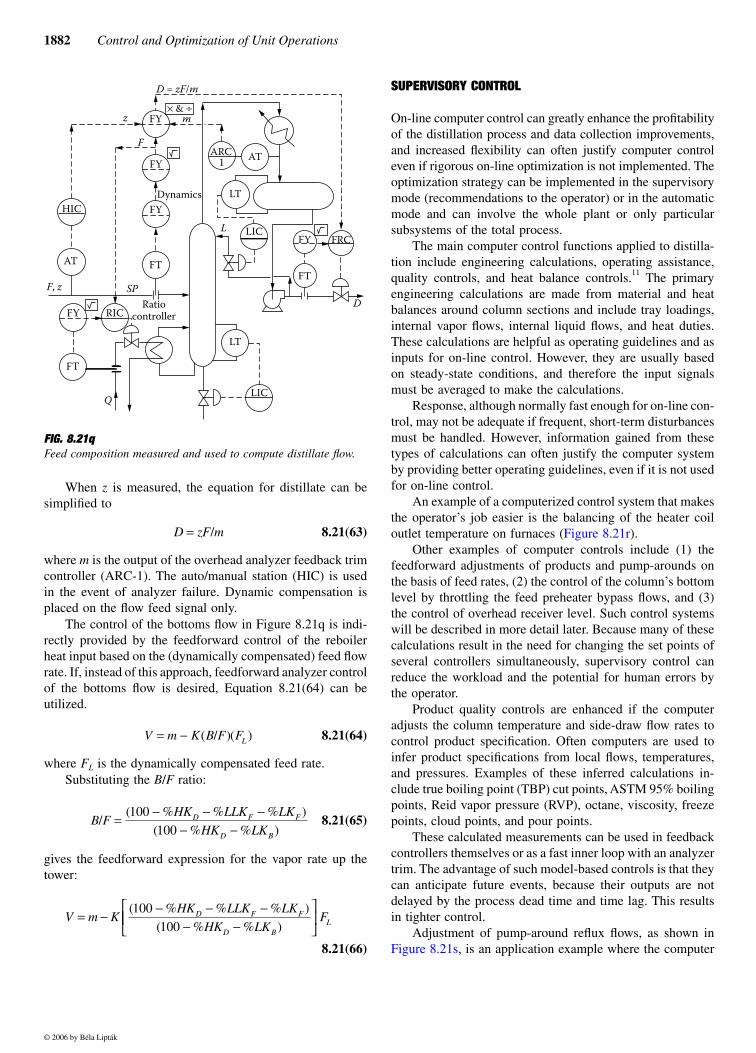
Occasionally, changes in feed composition occur too fast tobe handled by feedback control, and feedforward compensa-tion for these changes is necessary (Figure 8.21q).
The basic material balance equation, Equation 8.21(62),already has a term, z, representing concentration of the keycomponent in the feed:
8.21(62)
FIG. 8.21p The decoupling of a distillation tower when the compositions of both products are being controlled.
L = K1Q − K2F
FY
FYF L
Q Q
FY
X
AT
FRC FY
FTL
SP
F FY
FYFT
LT
ARC AT
LC
FIC FY FT
LIC
k X
Dynamics
(V/F)min + (V/F)
DynamicsARC
Σ
Q = kF [(V/F)]min+ (V/F)]
+K1
K2
−
D Fz xy x
= −−
© 2006 by Béla Lipták
1882 Control and Optimization of Unit Operations
When z is measured, the equation for distillate can besimplified to
8.21(63)
where m is the output of the overhead analyzer feedback trimcontroller (ARC-1). The auto/manual station (HIC) is usedin the event of analyzer failure. Dynamic compensation isplaced on the flow feed signal only.
The control of the bottoms flow in Figure 8.21q is indi-rectly provided by the feedforward control of the reboilerheat input based on the (dynamically compensated) feed flowrate. If, instead of this approach, feedforward analyzer controlof the bottoms flow is desired, Equation 8.21(64) can beutilized.
8.21(64)
where FL is the dynamically compensated feed rate.Substituting the B/F ratio:
8.21(65)
gives the feedforward expression for the vapor rate up thetower:
8.21(66)
SUPERVISORY CONTROL
On-line computer control can greatly enhance the profitabilityof the distillation process and data collection improvements,and increased flexibility can often justify computer controleven if rigorous on-line optimization is not implemented. Theoptimization strategy can be implemented in the supervisorymode (recommendations to the operator) or in the automaticmode and can involve the whole plant or only particularsubsystems of the total process.
The main computer control functions applied to distilla-tion include engineering calculations, operating assistance,quality controls, and heat balance controls.11 The primaryengineering calculations are made from material and heatbalances around column sections and include tray loadings,internal vapor flows, internal liquid flows, and heat duties.These calculations are helpful as operating guidelines and asinputs for on-line control. However, they are usually basedon steady-state conditions, and therefore the input signalsmust be averaged to make the calculations.
Response, although normally fast enough for on-line con-trol, may not be adequate if frequent, short-term disturbancesmust be handled. However, information gained from thesetypes of calculations can often justify the computer systemby providing better operating guidelines, even if it is not usedfor on-line control.
An example of a computerized control system that makesthe operator’s job easier is the balancing of the heater coiloutlet temperature on furnaces (Figure 8.21r).
Other examples of computer controls include (1) thefeedforward adjustments of products and pump-arounds onthe basis of feed rates, (2) the control of the column’s bottomlevel by throttling the feed preheater bypass flows, and (3)the control of overhead receiver level. Such control systemswill be described in more detail later. Because many of thesecalculations result in the need for changing the set points ofseveral controllers simultaneously, supervisory control canreduce the workload and the potential for human errors bythe operator.
Product quality controls are enhanced if the computeradjusts the column temperature and side-draw flow rates tocontrol product specification. Often computers are used toinfer product specifications from local flows, temperatures,and pressures. Examples of these inferred calculations in-clude true boiling point (TBP) cut points, ASTM 95% boilingpoints, Reid vapor pressure (RVP), octane, viscosity, freezepoints, cloud points, and pour points.
These calculated measurements can be used in feedbackcontrollers themselves or as a fast inner loop with an analyzertrim. The advantage of such model-based controls is that theycan anticipate future events, because their outputs are notdelayed by the process dead time and time lag. This resultsin tighter control.
Adjustment of pump-around reflux flows, as shown inFigure 8.21s, is an application example where the computer
FIG. 8.21q Feed composition measured and used to compute distillate flow.
HIC
z
D = zF/m
F
FY
FY× & ÷
m
FY
FT
RIC
LIC
LT
1 ATARC
FY
FT
D
L
SP
FRC
LIC
FY
F, z
FT
LT
Q
AT
Dynamics
Ratiocontroller
D zF m= /
V m K B F FL= − ( / )( )
B FHK LLK LK
HK LKD F F
D B
/( % % % )
( % % )=
− − −− −
100
100
V m KHK LLK LK
HK LKD F F
D B
= −− − −
− −
( % % % )
( % % )
100
100
FL
© 2006 by Béla Lipták
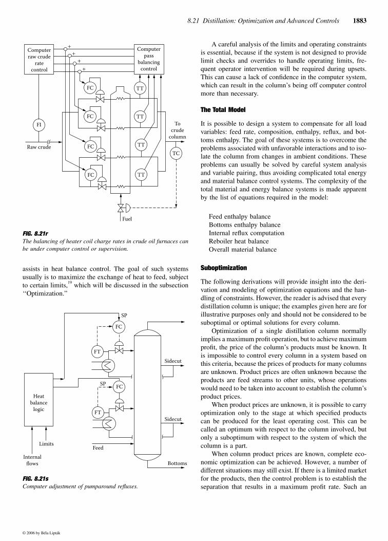
8.21 Distillation: Optimization and Advanced Controls 1883
assists in heat balance control. The goal of such systemsusually is to maximize the exchange of heat to feed, subjectto certain limits,19 which will be discussed in the subsection‘‘Optimization.”
A careful analysis of the limits and operating constraintsis essential, because if the system is not designed to providelimit checks and overrides to handle operating limits, fre-quent operator intervention will be required during upsets.This can cause a lack of confidence in the computer system,which can result in the column’s being off computer controlmore than necessary.
The Total Model
It is possible to design a system to compensate for all loadvariables: feed rate, composition, enthalpy, reflux, and bot-toms enthalpy. The goal of these systems is to overcome theproblems associated with unfavorable interactions and to iso-late the column from changes in ambient conditions. Theseproblems can usually be solved by careful system analysisand variable pairing, thus avoiding complicated total energyand material balance control systems. The complexity of thetotal material and energy balance systems is made apparentby the list of equations required in the model:
Feed enthalpy balanceBottoms enthalpy balanceInternal reflux computationReboiler heat balanceOverall material balance
Suboptimization
The following derivations will provide insight into the deri-vation and modeling of optimization equations and the han-dling of constraints. However, the reader is advised that everydistillation column is unique; the examples given here are forillustrative purposes only and should not be considered to besuboptimal or optimal solutions for every column.
Optimization of a single distillation column normallyimplies a maximum profit operation, but to achieve maximumprofit, the price of the column’s products must be known. Itis impossible to control every column in a system based onthis criteria, because the prices of products for many columnsare unknown. Product prices are often unknown because theproducts are feed streams to other units, whose operationswould need to be taken into account to establish the column’sproduct prices.
When product prices are unknown, it is possible to carryoptimization only to the stage at which specified productscan be produced for the least operating cost. This can becalled an optimum with respect to the column involved, butonly a suboptimum with respect to the system of which thecolumn is a part.
When column product prices are known, complete eco-nomic optimization can be achieved. However, a number ofdifferent situations may still exist. If there is a limited marketfor the products, then the control problem is to establish theseparation that results in a maximum profit rate. Such an
FIG. 8.21r The balancing of heater coil charge rates in crude oil furnaces canbe under computer control or supervision.
FIG. 8.21sComputer adjustment of pumparound refluxes.
Computerraw crude
ratecontrol
Computerpass
balancingcontrol
FC TT
TT
TT
TTFC
FC
FC
FI
Raw crudeTC
Tocrude
column
Fuel
++
++
Heatbalance
logic
FC
SP
FT
FCSP
Feed
Sidecut
Sidecut
Limits
Internalflows Bottoms
FT
© 2006 by Béla Lipták
1884 Control and Optimization of Unit Operations
optimum separation will be a function of all independentinputs to the column involved.
When an unlimited market exists for the products, andsufficient feedstock is available, the optimization problembecomes more difficult. Not only must the optimum separationbe established, but also the value of feed must be determined.Optimization for this case results in operating the column atmaximum loading or at maximum energy efficiency.
One of three possible constraints will be involved: Through-put will be limited by the overhead vapor condenser, thereboiler, or the column itself. In some cases, the constraintwill change from time to time, depending upon product pricesand other independent variables of the system. The design ofoptimal automatic control systems to single columns shouldfollow three logical steps:
1. Design the basic controls to regulate basic functions,such as pressures, temperatures, levels, and flows
2. Configure the controls to regulate the main sources ofheat inputs, including regulation of internal reflux flowrate, feed enthalpy, and reboiler heat flow rate
3. Apply controls to regulate the specified separation
A single column that is automated in this manner is calleda suboptimized system. This suboptimum is defined as anoperation that will produce close to the specified separation,whether or not that separation is ideal with regard to the totalsystem of which the column is a part. If product purities arehigher than specified, the operation cannot be consideredsuboptimum.
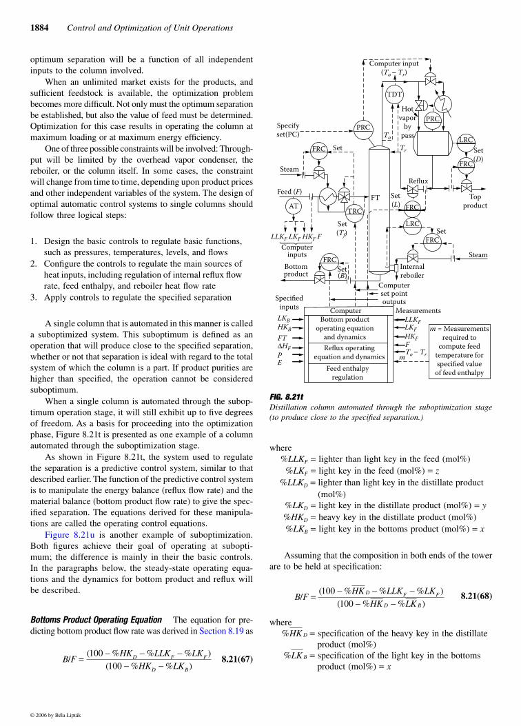
When a single column is automated through the subop-timum operation stage, it will still exhibit up to five degreesof freedom. As a basis for proceeding into the optimizationphase, Figure 8.21t is presented as one example of a columnautomated through the suboptimization stage.
As shown in Figure 8.21t, the system used to regulatethe separation is a predictive control system, similar to thatdescribed earlier. The function of the predictive control systemis to manipulate the energy balance (reflux flow rate) and thematerial balance (bottom product flow rate) to give the spec-ified separation. The equations derived for these manipula-tions are called the operating control equations.
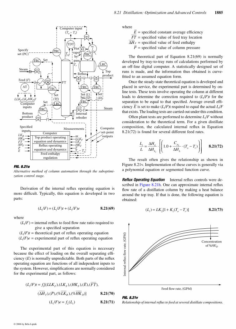
Figure 8.21u is another example of suboptimization.Both figures achieve their goal of operating at subopti-mum; the difference is mainly in their the basic controls.In the paragraphs below, the steady-state operating equa-tions and the dynamics for bottom product and reflux willbe described.
Bottoms Product Operating Equation The equation for pre-dicting bottom product flow rate was derived in Section 8.19 as
8.21(67)
where%LLKF = lighter than light key in the feed (mol%)
%LKF = light key in the feed (mol%) = z%LLKD = lighter than light key in the distillate product
(mol%)%LKD = light key in the distillate product (mol%) = y%HKD = heavy key in the distillate product (mol%)%LKB = light key in the bottoms product (mol%) = x
Assuming that the composition in both ends of the towerare to be held at specification:
8.21(68)
where= specification of the heavy key in the distillate
product (mol%)= specification of the light key in the bottoms
product (mol%) = xB F
HK LLK LK
HK LKD F F
D B
/( % % % )
( % % )=
− − −− −
100
100
FIG. 8.21t Distillation column automated through the suboptimization stage(to produce close to the specified separation.)
PRCPRC
Set
Specifyset(PC)
Steam
Feed (F)
ATTRC
FRC
FRC
TDT
LRC
FRC
Hotvapor
bypass
Computer input(To − Tr)
Set(D)
Set(L)
Set(Tf)
Set(B)
Topproduct
Reflux
Tr
To
FTFRC
LRCSet
Steam
FRC
Bottomproduct
Computerinputs
LLKF LKF HKF F
ComputerBottom product
operating equationand dynamicsReflux operating
equation and dynamicsFeed enthalpy
regulation
Specifiedinputs
LKB LLKFLKFHKFFTo − Trm
HKBFT∆HFPE
Measurements
m = Measurementsrequired to
compute feedtemperature forspecified value
of feed enthalpy
Computerset pointoutputs
Internalreboiler
B FHK LLK LK
HK LKD F F
D B/
( % % % )
( % % )=
− − −− −
100
100
%HK D
%LK B
© 2006 by Béla Lipták
8.21 Distillation: Optimization and Advanced Controls 1885
Derivation of the internal reflux operating equation ismore difficult. Typically, this equation is developed in twoparts:
8.21(69)
where(Li/F) = internal reflux to feed flow rate ratio required to
give a specified separation(Li/F)t = theoretical part of reflux operating equation(Li/F)e = experimental part of reflux operating equation
The experimental part of this equation is necessarybecause the effect of loading on the overall separating effi-ciency (E) is normally unpredictable. Both parts of the refluxoperating equation are functions of all independent inputs tothe system. However, simplifications are normally consideredfor the experimental part, as follows:
8.21(70)
8.21(71)
where= specified constant average efficiency= specified value of feed tray location= specified value of feed enthalpy= specified value of column pressure
The theoretical part of Equation 8.21(69) is normallydeveloped by tray-to-tray runs of calculations performed byan off-line digital computer. A statistically designed set ofruns is made, and the information thus obtained is curve-fitted to an assumed equation form.
Once the steady-state theoretical equation is developed andplaced in service, the experimental part is determined by on-line tests. These tests involve operating the column at differentloads to determine the correction required to (Li/F)t for theseparation to be equal to that specified. Average overall effi-ciency is set to make (Li/F)t required to equal the actual Li/Fthat exists. The loading tests are carried out under this condition.
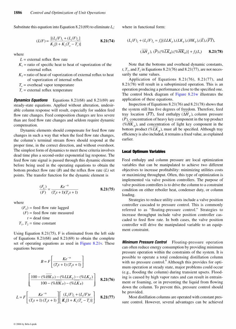
Often plant tests are performed to determine Li/F withoutconsideration to the theoretical term. For a given distillatecomposition, the calculated internal reflux in Equation8.21(72) is found for several different feed rates.
8.21(72)
The result often gives the relationship as shown inFigure 8.21v. Implementation of these curves is generally viaa polynomial equation or segmented function curve.
Reflux Operating Equation Internal reflux controls were de-scribed in Figure 8.21h. One can approximate internal refluxflow rate of a distillation column by making a heat balancearound the top tray. If that is done, the following equation isobtained:
8.21(73)
FIG. 8.21u Alternative method of column automation through the suboptimi-zation control stage.
PRCTo
TDT
LRC F
Computer input(To − Tr)
Specifyset (PC)
SetFRC
TRCATFT
Set(Tf)
Set
FRC
Steam
Feed (F)
Computerinputs
Bottomproduct
Specifiedinputs Measurements
Steam
Computerset-pointoutputs
Set (L)Set (Q)
Set(D)
Topproduct
PRC
LRC
Reflux
FRC
FRC
FRC
Hotvapor
by-passTr
Internalreboiler
ComputerTop product operatingequation and dynamics
Reflux operatingequation and dynamics
Feed enthalpyregulation
LKBHKB LLKFLKF
HKFF
m
To − Tr
FT∆HFPE
LLKF LKFHKF
( / ) ( / ) ( / )L F L F t L F ei i i= +
( / ) [( ),( ),( ),( ),( ),L F t f LLK LK HK E FTi F F F= 1
( ),( ),(% ),(% )]∆H P LK HKF B D
( / ) ( )L F e f Li i= 2
FIG. 8.21vRelationship of internal reflux to feed at several distillate compositions.
EFT
∆H F
P
E
L
L
H
H
C
HT Ti L
L
p
Lo r
i
L= ⋅ + ⋅ −
∆
∆ ∆1 0. ( )
( ) [ ( )]L LK K T Ti o r= + −2 11
Feed flow rate, (GPM)
Concentrationof %HKD
Inte
rnal
reflu
x flo
w ra
te, (
GPM
)
© 2006 by Béla Lipták
1886 Control and Optimization of Unit Operations
Substitute this equation into Equation 8.21(69) to eliminate Li:
8.21(74)
whereL = external reflux flow rate
K1 = ratio of specific heat to heat of vaporization of the external reflux
K2 = ratio of heat of vaporization of external reflux to heat of vaporization of internal reflux
To = overhead vapor temperatureTr = external reflux temperature
Dynamics Equations Equations 8.21(68) and 8.21(69) aresteady-state equations. Applied without alteration, undesir-able column response will result, especially for sudden feedflow rate changes. Feed composition changes are less severethan are feed flow rate changes and seldom require dynamiccompensation.
Dynamic elements should compensate for feed flow ratechanges in such a way that when the feed flow rate changes,the column’s terminal stream flows should respond at theproper time, in the correct direction, and without overshoot.The simplest form of dynamics to meet these criteria involvesdead time plus a second-order exponential lag response. Thefeed flow rate signal is passed through this dynamic elementbefore being used in the operating equations to obtain thebottom product flow rate (B) and the reflux flow rate (L) setpoints. The transfer function for the dynamic element is
8.21(75)
where(FL) = feed flow rate lagged(F) = feed flow rate measured
t = dead timeT1, T2 = time constant
Using Equation 8.21(75), F is eliminated from the left sideof Equations 8.21(68) and 8.21(69) to obtain the completeset of operating equations as used in Figure 8.21v. Theseequations become
8.21(76)
8.21(77)
where in functional form:
(FT),
(P),(%LKB),(%HKD)] + f2(Li) 8.21(78)
Note that the bottoms and overhead dynamic constants,t, T1, and T2 in Equations 8.21(76) and 8.21(77), are not neces-sarily the same values.
Application of Equations 8.21(76), 8.21(77), and8.21(78) will result in a suboptimized operation. This is anoperation producing a performance close to the specified one.The control block diagram of Figure 8.21w illustrates theapplication of these equations.
Inspection of Equations 8.21(76) and 8.21(78) shows thatthe system still has five degrees of freedom. Therefore, feedtray location (FT), feed enthalpy column pressure
concentration of heavy key component in the top productand concentration of light key component in the
bottom product must all be specified. Although trayefficiency is also included, it remains a fixed value, as explainedearlier.
Local Optimum Variables
Feed enthalpy and column pressure are local optimizationvariables that can be manipulated to achieve two differentobjectives to increase profitability: minimizing utilities costsor maximizing throughput. Often, this type of optimization isimplemented via valve position controllers. The purpose ofvalve position controllers is to drive the column to a constraintcondition on either reboiler heat, condenser duty, or columnloading.
Strategies to reduce utility costs include a valve positioncontroller cascaded to pressure control. This is commonlyreferred to as “floating-pressure control.” Strategies toincrease throughput include valve position controller cas-caded to feed flow rate. In both cases, the valve positioncontroller will drive the manipulated variable to an equip-ment constraint.
Minimum Pressure Control Floating-pressure operationcan often reduce energy consumption by providing minimumpressure operation within the constraints of the system. It ispossible to operate a total condensing distillation columnwith no pressure control.8 Although this provides for opti-mum operation at steady state, major problems could occur(e.g., flooding the column) during transient upsets. Flood-ing is caused by high vapor rates and can result in entrain-ment or foaming, or in preventing the liquid from flowingdown the column. To prevent this, pressure control shouldbe provided.
Most distillation columns are operated with constant pres-sure control. However, several advantages can be achieved
( / )[( / ) ( / ) ]
[ ( )]L F
L F L F
K K T Ti t i e
o r
=+
+ −2 11
( )
( ) ( )( )
F
FKe
T s T sL
ts
=+ +
−
1 21 1
B FKe
T s T s
ts
=+ +
−
( ) ( )1 21 1
100
100
− − −− −
(% ) (% ) (% )
(% ) (% )
HK LLK LK
HK LK
D F F
D B
L FKe
T s T s
L F L F etsi t i=
+ +
+−
( ) ( )
( / ) ( / )
1 21 1 KK K T To t2 11[ ( )]+ −
( / ) ( / ) [( ),( ),( ),( ),L F L F f LLK LK HK Ei t i e F F F+ = 1
( ),∆HF
( ),∆HF
( ),P(% ),HK
D
(% ),LKB
© 2006 by Béla Lipták
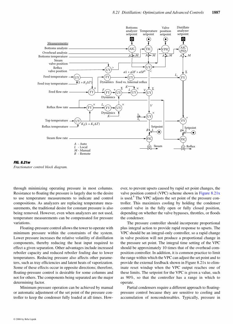
8.21 Distillation: Optimization and Advanced Controls 1887
through minimizing operating pressure in most columns.Resistance to floating the pressure is largely due to the desireto use temperature measurements to indicate and controlcompositions. As analyzers are replacing temperature mea-surements, the traditional desire for constant pressure is alsobeing removed. However, even when analyzers are not used,temperature measurements can be compensated for pressurevariations.
Floating-pressure control allows the tower to operate withminimum pressure within the constraints of the system.Lower pressure increases the relative volatility of distillationcomponents, thereby reducing the heat input required toeffect a given separation. Other advantages include increasedreboiler capacity and reduced reboiler fouling due to lowertemperatures. Reducing pressure also affects other parame-ters, such as tray efficiencies and latent heats of vaporization.Some of these effects occur in opposite directions; therefore,floating-pressure control is desirable for some columns andnot for others. The components being separated are the majordetermining factor.
Minimum pressure operation can be achieved by manualor automatic adjustment of the set point of the pressure con-troller to keep the condenser fully loaded at all times. How-
ever, to prevent upsets caused by rapid set point changes, thevalve position control (VPC) scheme shown in Figure 8.21xis used.8 The VPC adjusts the set point of the pressure con-troller. This maximizes cooling by holding the condensercontrol valve in the fully open or fully closed position,depending on whether the valve bypasses, throttles, or floodsthe condenser.
The pressure controller should incorporate proportionalplus integral action to provide rapid response to upsets. TheVPC should be an integral-only controller, so a rapid changein valve position will not produce a proportional change inthe pressure set point. The integral time setting of the VPCshould be approximately 10 times that of the overhead com-position controller. In addition, it is common practice to limitthe range within which the VPC can adjust the set point and toprovide the external feedback shown in Figure 8.21x to elim-inate reset windup when the VPC output reaches one ofthese limits. The setpoint for the VPC is given a value, suchas 90%, so that the controller has a range in which tooperate.
Partial condensers require a different approach to floating-pressure control because they are sensitive to cooling andaccumulation of noncondensables. Typically, pressure in
FIG. 8.21wFractionator control block diagram.
VPICTIC AICPIDAIC
UY
FY FYLi
AA MMA MA M
FY FY
FY
FYFY
UY
UY UY UY
UY
UY
FIC FIC
RefluxSteam
SetpointSetpoint
Dynamics
Dynamics
Dynamics Feed vs. Internal reflux
UY
UY
UY
Bottomsanalyzersetpoint
Temperaturesetpoint
Valvepositionsetpoint
Distillateanalyzersetpoint
Measurements:Bottoms analysis
Overhead analysisBottoms temperature
Steamvalve position
Refluxvalve position
Feed temperature
Feed tray temperature
Feed flow rate
Reflux flow rate
Top temperature
Reflux temperature
Steam flow rate
A - AutoL - LocalM - ManualR - Remote
<>
VF
K
KL
V
LR LR
Li
Σ
ΣΣ×
× ×
×
×
÷
+
K2(1 + K1∆T )
(1 + K2∆T )
a1 + a2F + a3F2
λbλs
•••••
•
••••••• • • •• •
© 2006 by Béla Lipták
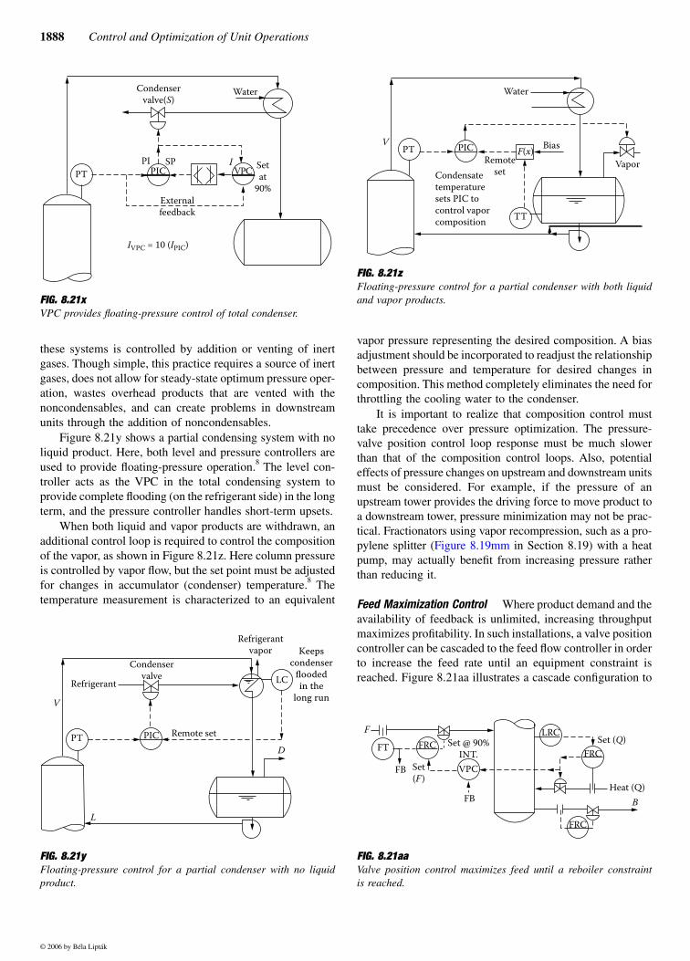
1888 Control and Optimization of Unit Operations
these systems is controlled by addition or venting of inertgases. Though simple, this practice requires a source of inertgases, does not allow for steady-state optimum pressure oper-ation, wastes overhead products that are vented with thenoncondensables, and can create problems in downstreamunits through the addition of noncondensables.
Figure 8.21y shows a partial condensing system with noliquid product. Here, both level and pressure controllers areused to provide floating-pressure operation.8 The level con-troller acts as the VPC in the total condensing system toprovide complete flooding (on the refrigerant side) in the longterm, and the pressure controller handles short-term upsets.
When both liquid and vapor products are withdrawn, anadditional control loop is required to control the compositionof the vapor, as shown in Figure 8.21z. Here column pressureis controlled by vapor flow, but the set point must be adjustedfor changes in accumulator (condenser) temperature.8 Thetemperature measurement is characterized to an equivalent
vapor pressure representing the desired composition. A biasadjustment should be incorporated to readjust the relationshipbetween pressure and temperature for desired changes incomposition. This method completely eliminates the need forthrottling the cooling water to the condenser.
It is important to realize that composition control musttake precedence over pressure optimization. The pressure-valve position control loop response must be much slowerthan that of the composition control loops. Also, potentialeffects of pressure changes on upstream and downstream unitsmust be considered. For example, if the pressure of anupstream tower provides the driving force to move product toa downstream tower, pressure minimization may not be prac-tical. Fractionators using vapor recompression, such as a pro-pylene splitter (Figure 8.19mm in Section 8.19) with a heatpump, may actually benefit from increasing pressure ratherthan reducing it.
Feed Maximization Control Where product demand and theavailability of feedback is unlimited, increasing throughputmaximizes profitability. In such installations, a valve positioncontroller can be cascaded to the feed flow controller in orderto increase the feed rate until an equipment constraint isreached. Figure 8.21aa illustrates a cascade configuration to
FIG. 8.21xVPC provides floating-pressure control of total condenser.
FIG. 8.21yFloating-pressure control for a partial condenser with no liquidproduct.
Condenservalve(S)
Water
VPCPI I
PIC
Externalfeedback
SP Setat
90%
IVPC = 10 (IPIC)
PT
PIC
V
L
D
LC
Refrigerantvapor
Condenservalve
Refrigerant
Remote set
Keepscondenser
floodedin the
long run
PT
FIG. 8.21zFloating-pressure control for a partial condenser with both liquidand vapor products.
FIG. 8.21aaValve position control maximizes feed until a reboiler constraintis reached.
PICVPT
TT
Bias
Water
VaporCondensatetemperaturesets PIC tocontrol vaporcomposition
F(x)Remote
set
FRCFT
VPC
FRC
FRC
LRCSet (Q)
Heat (Q)BFB
FB Set(F )
Set @ 90%INT.
F
© 2006 by Béla Lipták
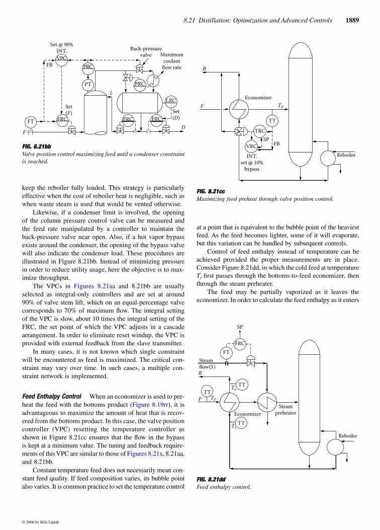
8.21 Distillation: Optimization and Advanced Controls 1889
keep the reboiler fully loaded. This strategy is particularlyeffective when the cost of reboiler heat is negligible, such aswhen waste steam is used that would be vented otherwise.
Likewise, if a condenser limit is involved, the openingof the column pressure control valve can be measured andthe feed rate manipulated by a controller to maintain theback-pressure valve near open. Also, if a hot vapor bypassexists around the condenser, the opening of the bypass valvewill also indicate the condenser load. These procedures areillustrated in Figure 8.21bb. Instead of minimizing pressurein order to reduce utility usage, here the objective is to max-imize throughput.
The VPCs in Figures 8.21aa and 8.21bb are usuallyselected as integral-only controllers and are set at around90% of valve stem lift, which on an equal-percentage valvecorresponds to 70% of maximum flow. The integral settingof the VPC is slow, about 10 times the integral setting of theFRC, the set point of which the VPC adjusts in a cascadearrangement. In order to eliminate reset windup, the VPC isprovided with external feedback from the slave transmitter.
In many cases, it is not known which single constraintwill be encountered as feed is maximized. The critical con-straint may vary over time. In such cases, a multiple con-straint network is implemented.
Feed Enthalpy Control When an economizer is used to pre-heat the feed with the bottoms product (Figure 8.19rr), it isadvantageous to maximize the amount of heat that is recov-ered from the bottoms product. In this case, the valve positioncontroller (VPC) resetting the temperature controller asshown in Figure 8.21cc ensures that the flow in the bypassis kept at a minimum value. The tuning and feedback require-ments of this VPC are similar to those of Figures 8.21x, 8.21aa,and 8.21bb.
Constant temperature feed does not necessarily mean con-stant feed quality. If feed composition varies, its bubble pointalso varies. It is common practice to set the temperature control
at a point that is equivalent to the bubble point of the heaviestfeed. As the feed becomes lighter, some of it will evaporate,but this variation can be handled by subsequent controls.
Control of feed enthalpy instead of temperature can beachieved provided the proper measurements are in place.Consider Figure 8.21dd, in which the cold feed at temperatureTf first passes through the bottoms-to-feed economizer, thenthrough the steam preheater.
The feed may be partially vaporized as it leaves theeconomizer. In order to calculate the feed enthalpy as it enters
FIG. 8.21bbValve position control maximizing feed until a condenser constraintis reached.
FRCFRCFT FRCSet(D)
Set(F )
D
LRC
Maximumcoolant
flow rate
Back-pressurevalve
PT
PRCFBVPC
Set @ 90%INT.
L
F
PRC
FIG. 8.21ccMaximizing feed preheat through valve position control.
FIG. 8.21ddFeed enthalpy control.
TRC
EconomizerTF
FB
ReboilerINT.set @ 10%
bypass
SP
TT
F
B
VRC
FRC
Steamflow(S )B
FTT
TT
TT
FT
TF
Te
Ti
Economizer
Reboiler
Steampreheater
SP
© 2006 by Béla Lipták
1890 Control and Optimization of Unit Operations
the column, the following heat balance can be written:
8.21(79)
where= feed enthalpy as it enters the tower, BTU/lb
(kcal/kg)F = feed flow to preheater, lb/h (kg/h)S = steam flow, lb/h (kg/h)
= feed heat capacity, BTU/lb°F (kcal/kg°C)= feed temperature before preheaters,°F (°C)
B = bottoms flow to economizer, lb/h (kg/h)= bottoms heat capacity, BTU/lb (kcal/kg)= bottoms temperature to economizer,°F (°C)= bottoms temperature after economizer,°F (°C)= steam heat of vaporization minus condensate
heat, BTU/lb°F (kcal/kg°C)
Rearranging Equation 8.21(79) gives
8.21(80)
or, solving for the manipulated variable, the steam flow thatwill provide constant feed enthalpy is
8.21(81)
The primary effect of increasing feed enthalpy is todecrease vapor-liquid circulation below the feed tray relativeto that above the feed tray. When feed preheat is less expensivethan reboiler heat, or when the reboiler is the limiting con-straint, maximum feed preheat is often optimal. When con-denser capacity is limiting, or flooding is encountered abovethe feed tray, preheat is not desired.
OPTIMIZATION
Optimization implies maximum profit rate. An objectivefunction is selected, and manipulated variables are chosenthat will maximize or minimize that function. This is similarto the PID equation that is designed to minimize the errorbetween the set point and measurement, but at a higher level.Optimization can be applied in several layers. Local optimi-zation is the optimization of a single column. Normally, thegoal of optimization of a single tower is to obtain minimumenergy consumption or maximum throughput.
Unit optimization addresses several columns in series orparallel. It is concerned with the effective allocation of feed-
stocks and energy among the members of that system. Plantwideoptimization involves coordinating the control of distillationunits, furnaces, compressors, and so on to maximize profit fromthe entire operation. All lower-level control functions respondto set points received from higher-level optimizers.
If Product Prices are Unknown
Unless the prices of terminal products of a distillation columnare known, it is impossible to maximize the profit rate forthat column without taking into account all other aspects ofthe overall plant of which the column is a part. Thus, opti-mization for a single distillation column whose terminalproduct prices are unknown is a matter of producing speci-fication products for minimum operating cost. Determiningthe optimum separation for the column requires optimizingthe overall system of which the column is a part.
Optimization of a single column whose product pricesare unknown involves determining the values for the locationof the feed tray (FT), for the feed enthal (∆HF), and forcolumn pressure that result in minimum operating costsfor whatever separation is specified. Any applicable mathe-matical approach can be used to establish values for (FT),(∆HF), and that will result in minimum operating costs.
Assuming that Equations 8.21(76), 8.21(77), and 8.21(78)are available, it is a relatively simple matter to establishoptimum values for these three variables that result in min-imum operating costs. Because these variables have specificconstraint values, one method involves a search technique.It is usually difficult to justify the search technique for on-line computer control. Therefore, a statistical design studycan be made off-line on another computer that allows cor-relation of the variables with each of the three optimizingvariables.
Theoretically, three equations in functional form describethe optimum for (FT), (∆HF), and
8.21(82)
8.21(83)
(P)o =
8.21(84)
In a majority of cases, the optimum for column pressure,will be the minimum value with constraints of the sys-
tem. Normally, can be lowered until the condenser capac-ity is reached, or until liquid entrainment in the vapor on thetrays is initiated.
( )( ) ( )( )( ) ( )( )( ) ( )(F H F C T B C T T SF p f p i eF B∆ ∆= + − + HHstm )
∆HF
CpF
Tf
CpB
Ti
Te
∆Hstm
∆ ∆H C T B F C T T S HF p f p i eF B= + − +( )( ) ( / )( )( ) ( )( )/stm FF
S F H C T B C T HF p f pF B= − −[ ( ) ( )]/∆ ∆ ∆ stm
( )P
( )P
( )P
( ) [(% ), (% ), (% ), ( ), (% ), (FT f LLK LK HK F HKo F F F D= 3 %% )]LK B
( ) [(% ), (% ), (% ), ( ),
(% ),
∆H f LLK LK HK F
HK
F o F F F
D
= 4
((% )]LK B
f LLK LK HK F HK LKF F F D B5[(% ),(% ),(% ),( ), (% ),(% )]
( ),P( )P
© 2006 by Béla Lipták
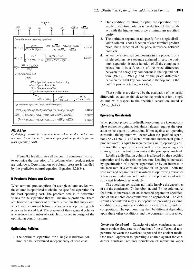
8.21 Distillation: Optimization and Advanced Controls 1891
Figure 8.21ee illustrates all the control equations involvedto optimize the operation of a column when product pricesare unknown. Determination of column pressure is handledby the predictive control equation, Equation 8.21(84).
If Products Prices are Known
When terminal product prices for a single column are known,the column is optimized to obtain the specified separation forthe least operating cost. The problem now is to determinevalues for the separation that will maximize profit rate. Thereare, however, a number of different situations that may exist,which will be covered below. Several general optimizing pol-icies can be stated first. The purpose of these general policiesis to reduce the number of variables involved in design of theoptimizing control system.
Optimizing Policies
1. The optimum separation for a single distillation col-umn can be determined independently of feed cost.
2. One condition resulting in optimized operation for asingle distillation column is production of that prod-uct with the highest unit price at minimum specifiedpurity.
3. The optimum separation to specify for a single distil-lation column is not a function of each terminal productprice, but a function of the price difference betweenproducts.
4. When the individual components in the products of asingle column have separate assigned prices, the opti-mum separation is not a function of all the componentprices but it is a function of the price differencebetween the heavy key component in the top and bot-tom (PHKD − PHKB) and of the price differencebetween the light key component in the top and in thebottom products (PLKD − PLKB).
These policies are derived by the evaluation of the partialdifferential equations that describe the profit rate for a singlecolumn with respect to the specified separation, noted as
Operating Constraints
When product prices for a distillation column are known, com-plete economic optimization almost always requires the oper-ation to be against a constraint. If not against an operatingconstraint, the optimum will occur when the specified separa-tion is of such a value that incremental gain inproduct worth is equal to incremental gain in operating cost.Because the majority of cases will involve operating con-straints, it is important to understand the principles involved.
Loading a distillation column is affected by the specifiedseparation and by the existing feed rate. Loading is increasedby specification of a better separation or by an increase inthe feed rate at a constant separation. In general, both thefeed rate and separation are involved as optimizing variableswhen an unlimited market exists for the products and whensufficient feedstock is available.
The operating constraints normally involve the capacitiesof (1) the condenser, (2) the reboiler, and (3) the column. Asfeed rate is increased, or an increased separation specified,one of these three constraints will be approached. The con-straint encountered may also depend on prevailing externalconditions, e.g., ambient conditions, steam pressure, and feedcomposition. The optimum may then be different dependingupon these other conditions and the constraint first reached.
Condenser Constraint Capacity of a given condenser at max-imum coolant flow rate is a function of the differential tem-perature between the overhead vapor and the coolant media.One useful approach to operating a column against the con-denser constraint requires correlation of maximum vapor
FIG. 8.21eeOptimizing control for single column when product prices areunknown (criterion is to produce specification products for theleast operating cost).
Suboptimization operating equations:
For liquid phase feed
(B) = (F )
(FT)o (Tf) (P)o(B) (L)
(L) = (F)
where
Setpoints
(%HKD) (%LKB)
Ke−ts
(T1s + 1) (T2s + 1)
Ke−ts
(T1s + 1) K2[1 + K1(To − Tr)](T2 s + 1)
100 − (%HKD) − (%LLKF) − (%LKF)100 − (%HKD) − (%LKB)
(Li/F)t − (Li/F )e
8.21(76)
8.21(77)
8.21(82)
8.21(83)
8.21(84)
(Tf) =(∆HF) + (CpF)(Tb)
∆HF = Specified value for feed enthalpy
(CpF)
(CpF) = Specific heat of feet(Tf) = Temperature of feed(Tb) = Base temperature of transmitter
(∆HF) = (∆HF)o
(P)ofor (Li/F )t
(FT )ofor (Li/F )t
Optimization equations (empirically developed)
(P)o = f5[(%LLKF), (%LKF), (%HKF), (F ), (%HKD), (%LKB)]
(FT )o = f3[(%LLKF), (%LKF), (%HKF), (F), (%HKD), (%LKB)]
(∆HF)o = f4[(%LLKF), (%LKF), (%HKF), (F ), (%HKD), (%LKB)]
( ), ( ).LK HKD B
( ), ( )LK HKB D
© 2006 by Béla Lipták
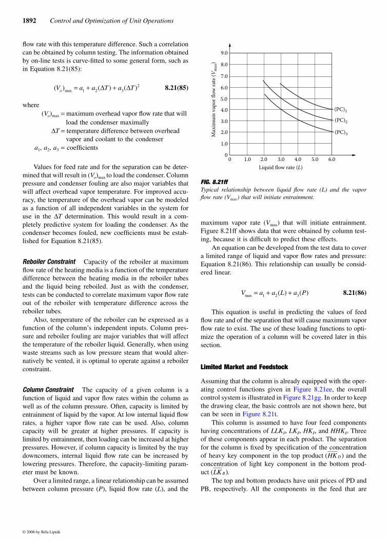
1892 Control and Optimization of Unit Operations
flow rate with this temperature difference. Such a correlationcan be obtained by column testing. The information obtainedby on-line tests is curve-fitted to some general form, such asin Equation 8.21(85):
8.21(85)
where(Vo)max = maximum overhead vapor flow rate that will
load the condenser maximally∆T = temperature difference between overhead
vapor and coolant to the condensera1, a2, a3 = coefficients
Values for feed rate and for the separation can be deter-mined that will result in (Vo)max to load the condenser. Columnpressure and condenser fouling are also major variables thatwill affect overhead vapor temperature. For improved accu-racy, the temperature of the overhead vapor can be modeledas a function of all independent variables in the system foruse in the ∆T determination. This would result in a com-pletely predictive system for loading the condenser. As thecondenser becomes fouled, new coefficients must be estab-lished for Equation 8.21(85).
Reboiler Constraint Capacity of the reboiler at maximumflow rate of the heating media is a function of the temperaturedifference between the heating media in the reboiler tubesand the liquid being reboiled. Just as with the condenser,tests can be conducted to correlate maximum vapor flow rateout of the reboiler with temperature difference across thereboiler tubes.
Also, temperature of the reboiler can be expressed as afunction of the column’s independent inputs. Column pres-sure and reboiler fouling are major variables that will affectthe temperature of the reboiler liquid. Generally, when usingwaste streams such as low pressure steam that would alter-natively be vented, it is optimal to operate against a reboilerconstraint.
Column Constraint The capacity of a given column is afunction of liquid and vapor flow rates within the column aswell as of the column pressure. Often, capacity is limited byentrainment of liquid by the vapor. At low internal liquid flowrates, a higher vapor flow rate can be used. Also, columncapacity will be greater at higher pressures. If capacity islimited by entrainment, then loading can be increased at higherpressures. However, if column capacity is limited by the traydowncomers, internal liquid flow rate can be increased bylowering pressures. Therefore, the capacity-limiting param-eter must be known.
Over a limited range, a linear relationship can be assumedbetween column pressure (P), liquid flow rate (L), and the
maximum vapor rate (Vmax) that will initiate entrainment.Figure 8.21ff shows data that were obtained by column test-ing, because it is difficult to predict these effects.
An equation can be developed from the test data to covera limited range of liquid and vapor flow rates and pressure:Equation 8.21(86). This relationship can usually be consid-ered linear.
8.21(86)
This equation is useful in predicting the values of feedflow rate and of the separation that will cause maximum vaporflow rate to exist. The use of these loading functions to opti-mize the operation of a column will be covered later in thissection.
Limited Market and Feedstock
Assuming that the column is already equipped with the oper-ating control functions given in Figure 8.21ee, the overallcontrol system is illustrated in Figure 8.21gg. In order to keepthe drawing clear, the basic controls are not shown here, butcan be seen in Figure 8.21t.
This column is assumed to have four feed componentshaving concentrations of LLKF, LKF, HKF, and HHKF. Threeof these components appear in each product. The separationfor the column is fixed by specification of the concentrationof heavy key component in the top product and theconcentration of light key component in the bottom prod-uct
The top and bottom products have unit prices of PD andPB, respectively. All the components in the feed that are
( ) ( ) ( )maxV a a T a To = + +1 2 32∆ ∆
FIG. 8.21ff Typical relationship between liquid flow rate (L) and the vaporflow rate (Vmax) that will initiate entrainment.
Max
imum
vap
or fl
ow ra
te (V
max
)
9.0
8.0
7.0
6.0
5.0
4.0
3.0
2.0
1.0
00 1.0 2.0 3.0 4.0 5.0 6.0
Liquid flow rate (L)
(PC)1
(PC)2
(PC)3
V a a L a Pmax ( ) ( )= + +1 2 3
( )HK D
( ).LK B
© 2006 by Béla Lipták
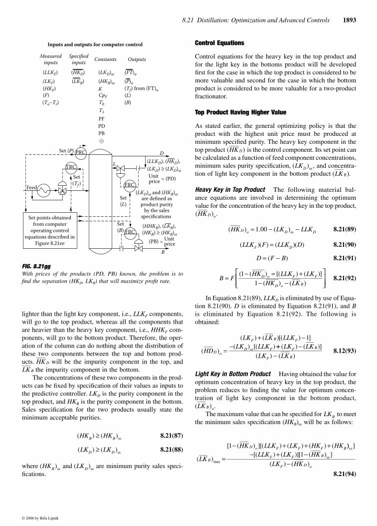
8.21 Distillation: Optimization and Advanced Controls 1893
lighter than the light key component, i.e., LLKF components,will go to the top product, whereas all the components thatare heavier than the heavy key component, i.e., HHKF com-ponents, will go to the bottom product. Therefore, the oper-ation of the column can do nothing about the distribution ofthese two components between the top and bottom prod-ucts. will be the impurity component in the top, and
the impurity component in the bottom. The concentrations of these two components in the prod-
ucts can be fixed by specification of their values as inputs tothe predictive controller. LKD is the purity component in thetop product, and HKB is the purity component in the bottom.Sales specification for the two products usually state theminimum acceptable purities.
8.21(87)
8.21(88)
where and are minimum purity sales speci-fications.
Control Equations
Control equations for the heavy key in the top product andfor the light key in the bottoms product will be developedfirst for the case in which the top product is considered to bemore valuable and second for the case in which the bottomproduct is considered to be more valuable for a two-productfractionator.
Top Product Having Higher Value
As stated earlier, the general optimizing policy is that theproduct with the highest unit price must be produced atminimum specified purity. The heavy key component in thetop product is the control component. Its set point canbe calculated as a function of feed component concentrations,minimum sales purity specification, and concentra-tion of light key component in the bottom product
Heavy Key in Top Product The following material bal-ance equations are involved in determining the optimumvalue for the concentration of the heavy key in the top product,
8.21(89)
8.21(90)
8.21(91)
8.21(92)
In Equation 8.21(89), LLKD is eliminated by use of Equa-tion 8.21(90). D is eliminated by Equation 8.21(91), and Bis eliminated by Equation 8.21(92). The following isobtained:
8.12(93)
Light Key in Bottom Product Having obtained the value foroptimum concentration of heavy key in the top product, theproblem reduces to finding the value for optimum concen-tration of light key component in the bottom product,
The maximum value that can be specified for to meetthe minimum sales specification (HKB)ss will be as follows:
8.21(94)
FIG. 8.21ggWith prices of the products (PD, PB) known, the problem is tofind the separation (HKD, LKB) that will maximize profit rate.
PRC
TRC
FRC
FRC
Inputs and outputs for computer control
Measuredinputs
Specifiedinputs Constants Outputs
(LLKF) (HKD) (FT)o(LKD)ss
(LKF) (LKB) (P)o(HKB)ss(HKF)
CpF
(Tf) from (FT)o
PF
(F)K
Tb
(L)(To−Tr)
T1
(B)
PDPB~
Feed
Set points obtainedfrom computer
operating controlequations described in
Figure 8.21ee
Set (P)
Set(Tf )
Set(L)
L
D
B
Set(B)
(LLKD), (HKD),
Unitprice = (PD)
(LKD) ≥ (LKD)ss
(LKD)ss and (HKB)ssare defined asproduct purity
by the salesspecifications
Unit
(HHKB), (LKB),
price
(HKB) ≥ (HKB)ss
(PB) =
HK D
LK B
( ) (HK HKB B≥ )ss
( ) (LK LKD D≥ )ss
(HKB)ss (LKD)ss
( )HK D
(LKD) ,ss
( ).LK B
( ) .HK D o
( ) . (HK LK LLKD o D D= − −1 00 )ss
( )( ) ( )( )LLK F LLK DF D=
D F B= −( )
B FHK LLK LK
HK LKD o F F
D o B=
− = +− −
( ( ) [( ) ( )]
( ) ( )
1
1
( )
( ) ( )[( ) ]( ) [( )
HD
LK LK LLKLK LLK
D o
F B F
D ss F=
+ −−
1++ −
−( ) ( )]
( ) ( )
LK LK
LK LKF B
F B
( ) .LK B o
LKB
( )
[ ( ) ][( ) ( ) ( ) (
maxLK
HK LLK LK HK HK
B
D o F F F B
=
− + + +1 )) ])
ss
ss− + −−
[( ) ( )][ ( ]
( ) ( )
LLK LK HK
LK HKF F B
F D o
1
© 2006 by Béla Lipták
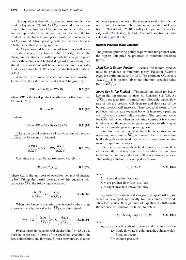
1894 Control and Optimization of Unit Operations
This equation is derived by the same procedure that wasused for Equation 8.21(94). As is lowered from its max-imum value, the flow rate of the bottom product will decreaseand the top product flow rate will increase. Because the topproduct is the highest unit price, profit will increase asis lowered. Also, operating costs will increase, becausea better separation is being specified.
As is lowered further, one of two things will occurto establish (the lowest value for LKB). Either thechange in operating cost will approach the change in profitrate, or the column will be loaded against an operating con-straint. This constraint will be a condenser limit, a reboilerlimit, or a column limit. Whichever occurs first will establish
Assume, for example, that no constraints are involved.In that case, the value of the products will be given by
8.21(95)
where PW is the total product worth rate, dollars/unit time.Eliminate B by
8.21(96)
to obtain
8.21(97)
Taking the partial derivative of this equation with respectto the following is obtained:
8.21(98)
Operating costs can be approximated closely by
8.21(99)
where CLi is the unit cost of operation per unit of internalreflux. Taking the partial derivative of this equation withrespect to the following is obtained:
8.21(100)
When the change in operating cost is equal to the changein product worth, the value for is determined.
8.21(101)
Evaluation of this equation will yield a value for Dmust be expressed in terms of the specified separation, thefeed composition, and flow rate. Li must be expressed in terms
of the independent inputs to the system as used in the internalreflux control equation. The simultaneous solution of Equa-tions 8.21(93) and 8.21(101) will yield optimum values forLKB and HKD: The total solution is indi-cated in Figure 8.21hh.
Bottom Product More Valuable
The general optimizing policy requires that the product withthe highest unit price be produced at minimum specifiedpurity.
Light Key in Bottom Product Because the bottom productmust be produced at minimum purity, Equation 8.21(94)gives the optimum value for The optimum equals
This, in turn, gives the minimum specified salespurity
Heavy Key in Top Product The maximum value for heavykey in the top product is given by Equation 8.21(93). As
is reduced from its maximum allowable value, flowrate of the top product will decrease and flow rate of thebottom product will increase. Therefore, total worth of theproducts will increase together but with increased operatingcosts due to increased reflux required. The optimum valuefor will occur when an operating constraint is encoun-tered or when the incremental gain in product worth is equalto the incremental gain in operating cost.
For this case, assume that the column approaches anoperating constraint as is lowered. Let this constraintbe flooding above the feed tray because of excessive entrain-ment of liquid in the vapor.
First, an equation needs to be developed for vapor flowrate above the feed tray in terms of variables that are con-tained in the bottom product and reflux operating equations.The loading equation is developed as follows:
8.21(102)
whereLi = internal reflux flow rateD = top product flow rate (distillate)Vt = vapor flow rate above feed tray
Vt can have a maximum value as given by Equation 8.21(86),which is developed specifically for the column involved.Therefore, equate the right side of Equation 8.21(86) withthe left side of Equation 8.21(102) to obtain
8.21(103)
wherea1, a2, a3 = coefficients of experimental loading equation
L = liquid flow rate in column at the point at which flooding occurs
P = column pressure
LK B
LK B
LK B
( )LK B o
( ) .LK B o
PW PD D PB B= +( )( ) ( )( )
B F D= −
PW PD PB D PB F+ − +( )( ) ( )( )
LK B ,
∂∂
= − ∂∂
( )( )
( )( )
( )PWLK
PD PBD
LKB B
( ) ( )( )OC CL Li i=
LK B ,
∂∂
= ∂∂
( )( )
( )( )
OCLK
CLLi
LKBi
B
( )LK B o
( )( )
( )
( )
( )PD PB
DLK
CLL
LKBi
i
B− ∂
∂
=∂
∂
( ) .LK B o
( ) , ( ) .LK HKB o D o
LK B. LK B
( ) .maxLK B
(HKB) .ss
HK D
HK D
HK D
L D Vi t+ =
L D a a L a Pi + = + +1 2 3( ) ( )
© 2006 by Béla Lipták
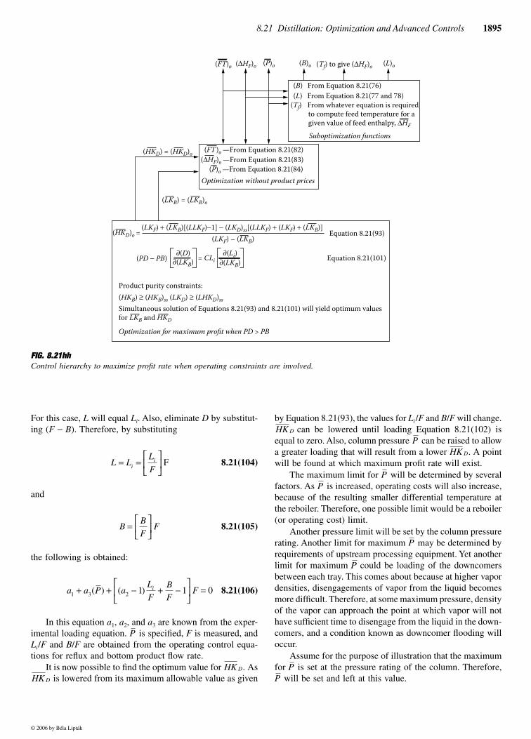
8.21 Distillation: Optimization and Advanced Controls 1895
For this case, L will equal Li. Also, eliminate D by substitut-ing (F − B). Therefore, by substituting
8.21(104)
and
8.21(105)
the following is obtained:
8.21(106)
In this equation a1, a2, and a3 are known from the exper-imental loading equation. is specified, F is measured, andLi/F and B/F are obtained from the operating control equa-tions for reflux and bottom product flow rate.
It is now possible to find the optimum value for Asis lowered from its maximum allowable value as given
by Equation 8.21(93), the values for Li/F and B/F will change.can be lowered until loading Equation 8.21(102) is
equal to zero. Also, column pressure can be raised to allowa greater loading that will result from a lower A pointwill be found at which maximum profit rate will exist.
The maximum limit for will be determined by severalfactors. As is increased, operating costs will also increase,because of the resulting smaller differential temperature atthe reboiler. Therefore, one possible limit would be a reboiler(or operating cost) limit.
Another pressure limit will be set by the column pressurerating. Another limit for maximum may be determined byrequirements of upstream processing equipment. Yet anotherlimit for maximum could be loading of the downcomersbetween each tray. This comes about because at higher vapordensities, disengagements of vapor from the liquid becomesmore difficult. Therefore, at some maximum pressure, densityof the vapor can approach the point at which vapor will nothave sufficient time to disengage from the liquid in the down-comers, and a condition known as downcomer flooding willoccur.
Assume for the purpose of illustration that the maximumfor is set at the pressure rating of the column. Therefore,
will be set and left at this value.
FIG. 8.21hhControl hierarchy to maximize profit rate when operating constraints are involved.
(FT)o (∆HF)o (P)o (L)o(B)o (Tf) to give (∆HF)o
(HKD) = (HKD)o
(LKB) = (LKB)o
(FT )o —From Equation 8.21(82)
(HKD)o =
(∆HF)o —From Equation 8.21(83)(P)o —From Equation 8.21(84)
Optimization without product prices
Optimization for maximum profit when PD > PB
(LKF) + (LKB)[(LLKF)−1] − (LKD)ss[(LLKF) + (LKF) + (LKB)](LKF) – (LKB)
Equation 8.21(93)
Equation 8.21(101)
Product purity constraints:
Simultaneous solution of Equations 8.21(93) and 8.21(101) will yield optimum valuesfor LKB and HKD
(PD − PB)∂(D) ∂(Li)
∂(LKB) ∂(LKB)= CLi
(HKB) ≥ (HKB)ss (LKD) ≥ (LHKD)ss
(B) From Equation 8.21(76)(L) From Equation 8.21(77 and 78)
(Tf) From whatever equation is required to compute feed temperature for a given value of feed enthalpy, ∆HF
Suboptimization functions
L LL
Fii= =
F
BBF
F=
a a P aL
FBF
Fi1 3 2 1 1 0+ + − + −
=( ) ( )
P
HK D.HK D
HK D
PHK D.
PP
P
P
PP
© 2006 by Béla Lipták
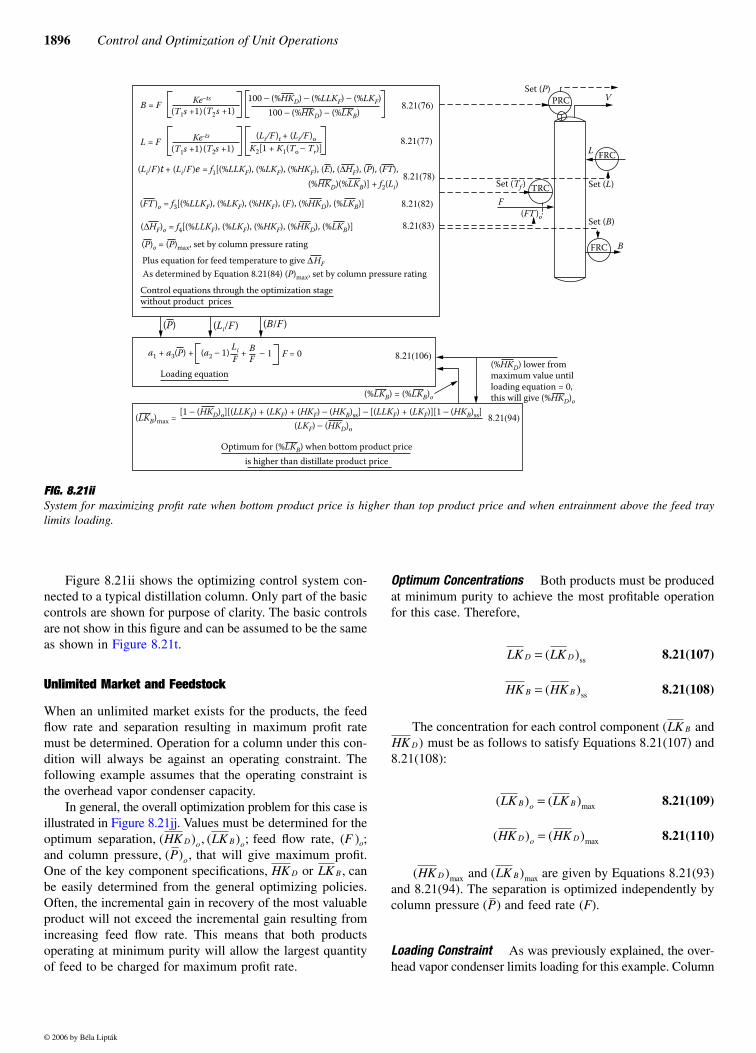
1896 Control and Optimization of Unit Operations
Figure 8.21ii shows the optimizing control system con-nected to a typical distillation column. Only part of the basiccontrols are shown for purpose of clarity. The basic controlsare not show in this figure and can be assumed to be the sameas shown in Figure 8.21t.
Unlimited Market and Feedstock
When an unlimited market exists for the products, the feedflow rate and separation resulting in maximum profit ratemust be determined. Operation for a column under this con-dition will always be against an operating constraint. Thefollowing example assumes that the operating constraint isthe overhead vapor condenser capacity.
In general, the overall optimization problem for this case isillustrated in Figure 8.21jj. Values must be determined for theoptimum separation, feed flow rate, (F )o;and column pressure, that will give maximum profit.One of the key component specifications, or canbe easily determined from the general optimizing policies.Often, the incremental gain in recovery of the most valuableproduct will not exceed the incremental gain resulting fromincreasing feed flow rate. This means that both productsoperating at minimum purity will allow the largest quantityof feed to be charged for maximum profit rate.
Optimum Concentrations Both products must be producedat minimum purity to achieve the most profitable operationfor this case. Therefore,
8.21(107)
8.21(108)
The concentration for each control component andmust be as follows to satisfy Equations 8.21(107) and
8.21(108):
8.21(109)
8.21(110)
and are given by Equations 8.21(93)and 8.21(94). The separation is optimized independently bycolumn pressure and feed rate (F).
Loading Constraint As was previously explained, the over-head vapor condenser limits loading for this example. Column
FIG. 8.21iiSystem for maximizing profit rate when bottom product price is higher than top product price and when entrainment above the feed traylimits loading.
B = F
L = F
Ke−ts
(T1s +1)(T2s +1)
Ke-ts
(T1s +1)(T2s +1)
100 − (%HKD) − (%LLKF) − (%LKF) 100 − (%HKD) − (%LKB)
8.21(76)
8.21(78)
8.21(82)
8.21(83)
8.21(106)
8.21(94)
8.21(77)(Li/F )t + (Li/F )o
(Li/F )t + (Li/F )e = f1[(%LLKF), (%LKF), (%HKF), (E), (∆HF), (P), (FT),(%HKD)(%LKB)] + f2(Li)
K2[1 + K1(To − Tr)]
(FT )o = f3[(%LLKF), (%LKF), (%HKF), (F ), (%HKD), (%LKB)]
(∆HF)o = f4[(%LLKF), (%LKF), (%HKF), (%HKD), (%LKB)]
(P)o = (P)max, set by column pressure rating Plus equation for feed temperature to give ∆HFAs determined by Equation 8.21(84) (P)max, set by column pressure rating
Control equations through the optimization stagewithout product prices
(P) (Li/F ) (B/F )
PRC
FRC
Set (L)
Set (B)
TRCF
(FT )o
FRC B
V
L
Set (P)
Set (Tf )
a1 + a3(P) + (a2 − 1) Li BFF + − 1 F = 0
Loading equation
(%LKB) = (%LKB)o
(%HKD) lower frommaximum value untilloading equation = 0,this will give (%HKD)o
(LKB)max = [1 − (HKD)o][(LLKF) + (LKF) + (HKF) − (HKB)ss] − [(LLKF) + (LKF)][1 − (HKB)ss] (LKF) − (HKD)o
Optimum for (%LKB) when bottom product priceis higher than distillate product price
( ) , ( ) ;HK LKD o B o
( ) ,P o
HK D LK B ,
LK LKD D= ( )ss
HK HKB B= ( )ss
(LK B
HK D)
( ) ( )maxLK LKB o B=
( ) ( )maxHK HKD o D=
( )maxHK D ( )maxLK B
( )P
© 2006 by Béla Lipták
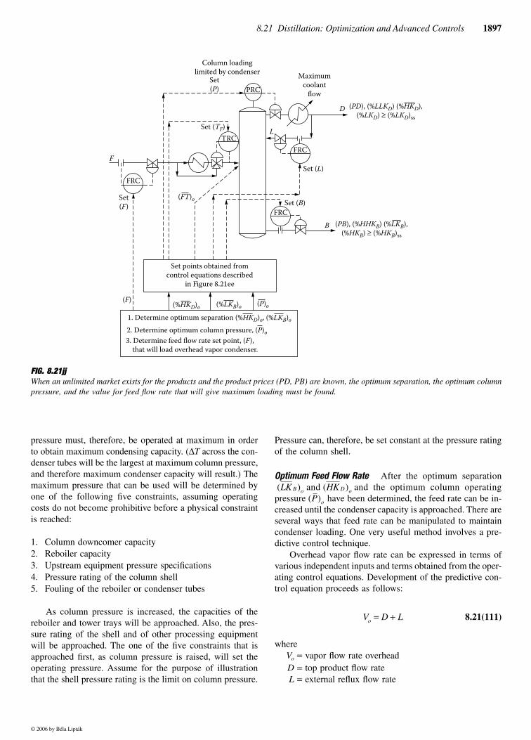
8.21 Distillation: Optimization and Advanced Controls 1897
pressure must, therefore, be operated at maximum in orderto obtain maximum condensing capacity. (∆T across the con-denser tubes will be the largest at maximum column pressure,and therefore maximum condenser capacity will result.) Themaximum pressure that can be used will be determined byone of the following five constraints, assuming operatingcosts do not become prohibitive before a physical constraintis reached:
1. Column downcomer capacity2. Reboiler capacity3. Upstream equipment pressure specifications4. Pressure rating of the column shell5. Fouling of the reboiler or condenser tubes
As column pressure is increased, the capacities of thereboiler and tower trays will be approached. Also, the pres-sure rating of the shell and of other processing equipmentwill be approached. The one of the five constraints that isapproached first, as column pressure is raised, will set theoperating pressure. Assume for the purpose of illustrationthat the shell pressure rating is the limit on column pressure.
Pressure can, therefore, be set constant at the pressure ratingof the column shell.
Optimum Feed Flow Rate After the optimum separationand and the optimum column operating
pressure have been determined, the feed rate can be in-creased until the condenser capacity is approached. There areseveral ways that feed rate can be manipulated to maintaincondenser loading. One very useful method involves a pre-dictive control technique.
Overhead vapor flow rate can be expressed in terms ofvarious independent inputs and terms obtained from the oper-ating control equations. Development of the predictive con-trol equation proceeds as follows:
8.21(111)
whereVo = vapor flow rate overheadD = top product flow rateL = external reflux flow rate
FIG. 8.21jjWhen an unlimited market exists for the products and the product prices (PD, PB) are known, the optimum separation, the optimum columnpressure, and the value for feed flow rate that will give maximum loading must be found.
PRC
TRC
FRC
FRC
FRC
Set (L)
Set (B)
L
F
(FT)o
B
Column loadinglimited by condenser
Set(P)
Set(F)
Set (TF)
Maximumcoolant
flow(PD), (%LLKD) (%HKD),
(%LKD) ≥ (%LKD)ss
(PB), (%HHKB) (%LKB),(%HKB) ≥ (%HKB)ss
D
Set points obtained fromcontrol equations described
in Figure 8.21ee
(F) (%HKD)o (%LKB)o (P)o
1. Determine optimum separation (%HKD)o, (%LKB)o 2. Determine optimum column pressure, (P)o3. Determine feed flow rate set point, (F),
that will load overhead vapor condenser.
( )LK B o ( )HK D o
( )P o
V D Lo = +
© 2006 by Béla Lipták
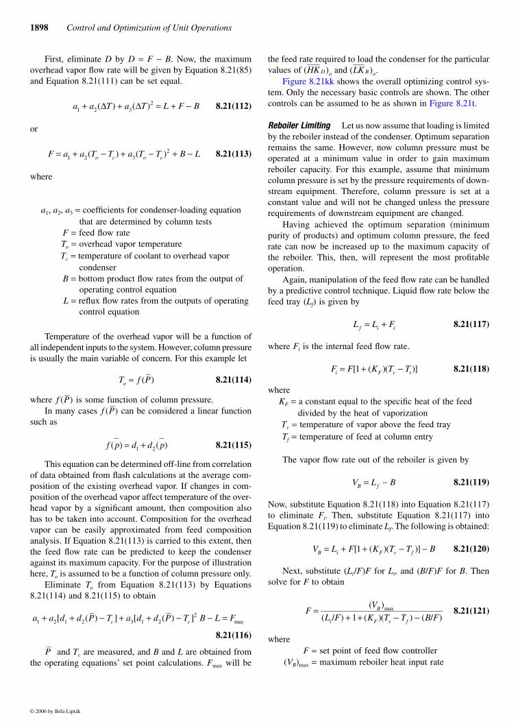
1898 Control and Optimization of Unit Operations
First, eliminate D by D = F − B. Now, the maximumoverhead vapor flow rate will be given by Equation 8.21(85)and Equation 8.21(111) can be set equal.
8.21(112)
or
8.21(113)
where
a1, a2, a3 = coefficients for condenser-loading equation that are determined by column tests
F = feed flow rateTo = overhead vapor temperatureTc = temperature of coolant to overhead vapor
condenserB = bottom product flow rates from the output of
operating control equationL = reflux flow rates from the outputs of operating
control equation
Temperature of the overhead vapor will be a function ofall independent inputs to the system. However, column pressureis usually the main variable of concern. For this example let
8.21(114)
where is some function of column pressure.In many cases can be considered a linear function
such as
8.21(115)
This equation can be determined off-line from correlationof data obtained from flash calculations at the average com-position of the existing overhead vapor. If changes in com-position of the overhead vapor affect temperature of the over-head vapor by a significant amount, then composition alsohas to be taken into account. Composition for the overheadvapor can be easily approximated from feed compositionanalysis. If Equation 8.21(113) is carried to this extent, thenthe feed flow rate can be predicted to keep the condenseragainst its maximum capacity. For the purpose of illustrationhere, To is assumed to be a function of column pressure only.
Eliminate To from Equation 8.21(113) by Equations8.21(114) and 8.21(115) to obtain
8.21(116)
and Tc are measured, and B and L are obtained fromthe operating equations’ set point calculations. Fmax will be
the feed rate required to load the condenser for the particularvalues of and
Figure 8.21kk shows the overall optimizing control sys-tem. Only the necessary basic controls are shown. The othercontrols can be assumed to be as shown in Figure 8.21t.
Reboiler Limiting Let us now assume that loading is limitedby the reboiler instead of the condenser. Optimum separationremains the same. However, now column pressure must beoperated at a minimum value in order to gain maximumreboiler capacity. For this example, assume that minimumcolumn pressure is set by the pressure requirements of down-stream equipment. Therefore, column pressure is set at aconstant value and will not be changed unless the pressurerequirements of downstream equipment are changed.
Having achieved the optimum separation (minimumpurity of products) and optimum column pressure, the feedrate can now be increased up to the maximum capacity ofthe reboiler. This, then, will represent the most profitableoperation.
Again, manipulation of the feed flow rate can be handledby a predictive control technique. Liquid flow rate below thefeed tray (Lf) is given by
8.21(117)
where Fi is the internal feed flow rate.
8.21(118)
whereKF = a constant equal to the specific heat of the feed
divided by the heat of vaporizationTv = temperature of vapor above the feed trayTf = temperature of feed at column entry
The vapor flow rate out of the reboiler is given by
8.21(119)
Now, substitute Equation 8.21(118) into Equation 8.21(117)to eliminate Fi. Then, substitute Equation 8.21(117) intoEquation 8.21(119) to eliminate Lf. The following is obtained:
8.21(120)
Next, substitute (Li/F)F for Li, and (B/F)F for B. Thensolve for F to obtain
8.21(121)
whereF = set point of feed flow controller
(VB)max = maximum reboiler heat input rate
a a T a T L F B1 2 32+ + = + −( ) ( )∆ ∆
F a a T T a T T B Lo c o c= + − + − + −1 2 32( ) ( )
T f Po = ( )
f P( )f P( )
f p d d p( ) ( )= +1 2
a a d d P T a d d P T B L Fc c1 2 1 2 3 1 22+ + − + + − − =[ ( ) ] [ ( ) ] max
P
( )HK D o ( ) .LK B o
L L Ff i i= +
F F K T Ti F v t= + −[ ( )( )]1
V L BB f= −
V L F K T T BB i F v f= + + − −[ ( )( )]1
FV
L F K T T B FB
i F v f
=+ + − −
( )
( / ) ( )( ) ( / )max
1
© 2006 by Béla Lipták
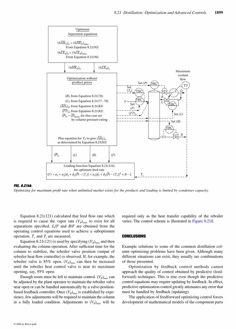
8.21 Distillation: Optimization and Advanced Controls 1899
Equation 8.21(121) calculated that feed flow rate whichis required to cause the vapor rate (VB)max to exist for allseparations specified. Li/F and B/F are obtained from theoperating control equations used to achieve a suboptimumoperation. Tv and Tf are measured.
Equation 8.21(121) is used by specifying (VB)max and thenevaluating the column operation. After sufficient time for thecolumn to stabilize, the reboiler valve position (output ofreboiler heat flow controller) is observed. If, for example, thereboiler valve is 85% open, (VB)max can then be increaseduntil the reboiler heat control valve is near its maximumopening, say, 95% open.
Enough room must be left to maintain control. (VB)max canbe adjusted by the plant operator to maintain the reboiler valvenear open or can be handled automatically by a valve-position-based feedback controller. Once (VB)max is established by expe-rience, few adjustments will be required to maintain the columnin a fully loaded condition. Adjustments to (VB)max will be
required only as the heat transfer capability of the reboilervaries. The control scheme is illustrated in Figure 8.21ll.
CONCLUSIONS
Example solutions to some of the common distillation col-umn optimizing problems have been given. Although manydifferent situations can exist, they usually are combinationsof those presented.
Optimization by feedback control methods cannotapproach the quality of control obtained by predictive (feed-forward) techniques. This is true even though the predictivecontrol equations may require updating by feedback. In effect,predictive optimization control greatly attenuates any error thatmust be handled by feedback (updating).
The application of feedforward optimizing control forcesdevelopment of mathematical models of the component parts
FIG. 8.21kkOptimizing for maximum profit rate when unlimited market exists for the products and loading is limited by condenser capacity.
FRCF
(F)(B)(L)
Loading function Equation 8.21(116)for optimum feed rate
TRC
OptimumSeparation equations
(%LKB)o = (%LKB)max
(%HKD)o = (%HKD)maxFrom Equation 8.21(93)
From Equation 8.21(94)
(%HKD)o (%LKB)o
Set (P)
Set (L)
Set (B)
Set(F)
Set(TF)
(FT)o
(P)o
Tc
PRC
FRC
FRC
TTD
RL
B
Maximumcoolant
flow
(F ) = a1 + a2[d1 + d2(P) − (Tc)] + a3[d1 + d2(P) − (Tc)]2 + B − L
Optimization withoutproduct prices
(B), from Equation 8.21(76)(L), from Equation 8.21(77–78)
Plus equation for TF to give (∆HF)oas determined by Equation 8.21(83)
(∆HF)o, from Equation 8.21(83)(FT)o, from Equation 8.21(82)(P)o = (P)max, for this case set
by column pressure rating
© 2006 by Béla Lipták
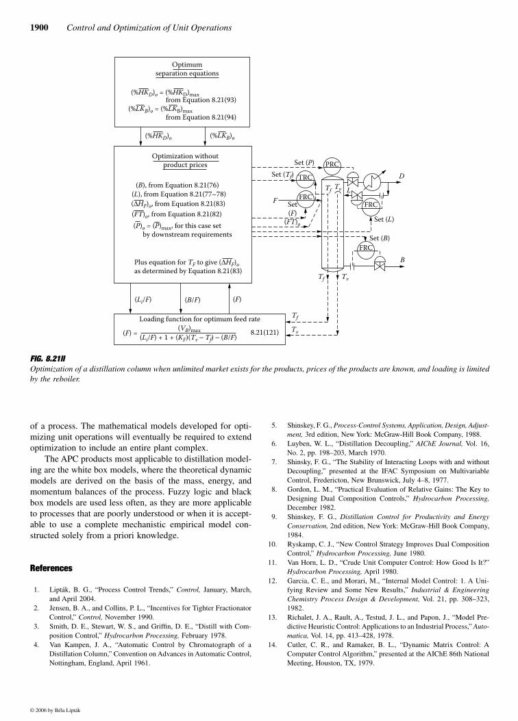
1900 Control and Optimization of Unit Operations
of a process. The mathematical models developed for opti-mizing unit operations will eventually be required to extendoptimization to include an entire plant complex.
The APC products most applicable to distillation model-ing are the white box models, where the theoretical dynamicmodels are derived on the basis of the mass, energy, andmomentum balances of the process. Fuzzy logic and blackbox models are used less often, as they are more applicableto processes that are poorly understood or when it is accept-able to use a complete mechanistic empirical model con-structed solely from a priori knowledge.
References
1. Lipták, B. G., “Process Control Trends,” Control, January, March,and April 2004.
2. Jensen, B. A., and Collins, P. L., “Incentives for Tighter FractionatorControl,” Control, November 1990.
3. Smith, D. E., Stewart, W. S., and Griffin, D. E., “Distill with Com-position Control,” Hydrocarbon Processing, February 1978.
4. Van Kampen, J. A., “Automatic Control by Chromatograph of aDistillation Column,” Convention on Advances in Automatic Control,Nottingham, England, April 1961.
5. Shinskey, F. G., Process-Control Systems, Application, Design, Adjust-ment, 3rd edition, New York: McGraw-Hill Book Company, 1988.
6. Luyben, W. L., “Distillation Decoupling,” AIChE Journal, Vol. 16,No. 2, pp. 198–203, March 1970.
7. Shinsky, F. G., “The Stability of Interacting Loops with and withoutDecoupling,” presented at the IFAC Symposium on MultivariableControl, Fredericton, New Brunswick, July 4–8, 1977.
8. Gordon, L. M., “Practical Evaluation of Relative Gains: The Key toDesigning Dual Composition Controls,” Hydrocarbon Processing,December 1982.
9. Shinskey, F. G., Distillation Control for Productivity and EnergyConservation, 2nd edition, New York: McGraw-Hill Book Company,1984.
10. Ryskamp, C. J., “New Control Strategy Improves Dual CompositionControl,” Hydrocarbon Processing, June 1980.
11. Van Horn, L. D., “Crude Unit Computer Control: How Good Is It?”Hydrocarbon Processing, April 1980.
12. Garcia, C. E., and Morari, M., “Internal Model Control: 1. A Uni-fying Review and Some New Results,” Industrial & EngineeringChemistry Process Design & Development, Vol. 21, pp. 308–323,1982.
13. Richalet, J. A., Rault, A., Testud, J. L., and Papon, J., “Model Pre-dictive Heuristic Control: Applications to an Industrial Process,” Auto-matica, Vol. 14, pp. 413–428, 1978.
14. Cutler, C. R., and Ramaker, B. L., “Dynamic Matrix Control: AComputer Control Algorithm,” presented at the AIChE 86th NationalMeeting, Houston, TX, 1979.
FIG. 8.21llOptimization of a distillation column when unlimited market exists for the products, prices of the products are known, and loading is limitedby the reboiler.
PRC
FRCFL
TRC
FRC
FRCB
Set (L)
D
Set (B)
Optimumseparation equations
(%HKD)o = (%HKD)max
(%LKB)o = (%LKB)max
from Equation 8.21(93)
from Equation 8.21(94)
(%HKD)o (%LKB)o
Optimization withoutproduct prices
(B), from Equation 8.21(76)(L), from Equation 8.21(77–78)
(FT)o, from Equation 8.21(82)(∆HF)o, from Equation 8.21(83)
Plus equation for TF to give (∆HF)oas determined by Equation 8.21(83)
(P)o = (P)max, for this case set by downstream requirements
(Li/F) (B/F) (F)
Loading function for optimum feed rate
(F) = (Li/F) + 1 + (KF)(Tv − Tf) − (B/F)(VB)max 8.21(121) Tv
Tv
TvTf
Tf
Tf
Set (P)Set (Tf)
Set(F)
(FT)o
© 2006 by Béla Lipták
8.21 Distillation: Optimization and Advanced Controls 1901
15. Singh, D. K., “Neural Network Model-Based Control of ChemicalProcesses,” Proceedings of the ISA/90 International Conference andExhibit, Part 2, New Orleans, LA, October 1990, pp. 965–968.
16. Douglas, J. M., Jafarey, A., and McAvoy, T. J., “Short-Cut Techniquesfor Distillation Column Design and Control, Part 1: Column Design,”I&EC Process Design and Development, Vol. 18, pp. 197–202, April1979.
17. Lee, P. L., and Sullivan, G. R., “Generic Model Control,” Computersand Chemical Engineering, Vol. 12, p. 573, 1988.
18. Tai, H. M., Wang, J., and Ashenayi, K., “A Neural Network TrackingController for High-Performance Applications,” Proceedings of theOklahoma Symposium on Artificial Intelligence, November 1991,p. 225.
19. Bannon, R. et al., “Heat Recovery in Hydrocarbon Distillation,”Chemical Engineering Progress, July 1978.
Bibliography
For pre-1990 literature, refer to Section 8.19
1990
Cingara, A., Jovanovic, M., and Mitrovic, M., “Analytical First-OrderDynamic Model of Binary Distillation Column,” Chemical Engineer-ing Science, Vol. 45, No. 12, pp. 3585–3592, 1990.
Ding, S. S. and Luyben, W. L., “Control of a Heat-Integrated ComplexDistillation Configuration,” Industrial & Engineering ChemistryResearch, No. 29, p. 1240, 1990.
Farrel, R. J. and Polli, A., “Comparison of Unconstrained Dynamic MatrixControl to Conventional Feedback Control for a First Order System,”Proceedings of the ISA/90 International Conference and Exhibit, Part2, New Orleans, LA, October 1990, pp. 1037–1046.
Gerstle, J. G., Hokanson, D. A., and Anderson, B. O., “Multivariable Controlof a C2 Splitter,” Proceedings of the AIChE Annual Meeting, Chicago,IL, November 1990.
Kister, H. Z., Distillation Operation, New York: McGraw-Hill Book Com-pany, 1990.
Li, R., Olson, J. H., and Chester, D. L., “Dynamic Fault Detection andDiagnosis Using Neural Networks,” Proceedings of the Fifth IEEEInternational Symposium on Intelligent Control, Philadelphia, PA,September 1990, pp. 1169–1174.
Papastathopoulou, H. S. and Luyben, W. L., “Potential Pitfalls in RatioControl Schemes,” Industrial & Engineering Chemistry Research,October 1990, pp. 2044–2053.
Pitt, M. J., Instrumentation and Automation in Process Control, New York:E. Horwood, 1990.
Riggs, J. B., “Advanced Model-Based Control of a Sidestream Draw Col-umn,” Proceedings of the ISA/90 International Conference and Exhibit,Part 2, New Orleans, LA, October 1990, pp. 1023–1032.
Riggs, J. B., Watts, J., and Beauford, M., “Industrial Experience with Apply-ing Nonlinear Process Model-Based Control to Distillation Columns,”Proceedings of the ISA/90 International Conference and Exhibit, Part2, New Orleans, LA, October 1990, pp. 1047–1054.
Skogestad, S., Jacobsen, E. W., and Morari, M., “Inadequacy of Steady-State Analysis for Feedback Control, Distillate, Bottom Control ofDistillation Columns,” Industrial & Engineering Chemistry Research,December 1990, pp. 2339–2346.
1991
Coughanowr, D. R., Process Systems Analysis and Control, 2nd edition,New York: McGraw-Hill Book Company, 1991.
Farhat, S., Piouleau, L., Domenech, S., and Czernicki, M., “Optimal Controlof Batch Distillation via Nonlinear Programming,” Chemical Engi-neering and Processing, Vol. 29, No. 1, pp. 33–38, January 1991.
Figuerosa, J. L., Desages, A. C., Romagnoli, J. A., and Palazoglu, “HighlyStructured Stability Margins for Process Control Systems. A CaseStudy of Decoupling Control in Distillation,” Computers & ChemicalEngineering, Vol. 15, No. 7, pp. 493–502, July 1991.
Gerstle, J. G. and Hokanson, D. A., “Experiences with Applying DynamicMatrix Control in Olefins Plants,” Proceedings of the ISA/91 Inter-national Conference and Exhibit, Part 1, Anaheim, CA, October1991.
Houk, B. G., Snowden, D. L., and Stevenson, T. E., “Improved Control ofEthylene Recovery Train Using Dynamic Matrix Control,” Proceed-ings of the ISA/91 International Conference and Exhibit, Part 1, Ana-heim, CA, October 1991.
Jacobsen, E. W., and Skogestad, S., “Control of Unstable Distillation Col-umns,” Proceedings of the American Control Conference, Green Val-ley, AZ, Vol. 1, pp. 773–778, 1991.
Jensen, B. A., “Improve Control of Cryogenic Gas Plants,” HydrocarbonProcessing, May 1991.
Kettinger, J. G., Gaines, L. D., and McGee, N. F., “Multivariable Control aDepropanizer,” Proceedings of the ISA/91 International Conferenceand Exhibit, Part 1, Anaheim, CA, October 1991.
O’Connor, D. L., Grimstad, K., and McKay, J., “Application of a SingleMultivariable Controller to Two Hydrocracker Distillation Columns inSeries,” Proceedings of the ISA/91 International Conference andExhibit, Part 1, Anaheim, CA, October 1991.
Papadopoulos, M. N. and Berkowitz, P. N., “Multivariable (MVC) ProcessControl. A User-Based On-Line Optimal Control System,” Proceed-ings of the Industrial Computing Conference, Anaheim, CA, October1991.
Papastathopoulou, H. S. and Luyben, W. L., “Control of a Binary Side-Stream Distillation Column,” Industrial & Engineering ChemistryResearch, April 1991, pp. 705–713.
Patwardhan, A. A. and Edgar, T. F., “Nonlinear Model-Predictive Controlof a Packed Distillation Column,” Proceedings of the American ControlConference, Green Valley, AZ, Vol. 1, 1991, pp. 767–772.
Radhakrishnan, T. K., and Gangiah, K., “Critical Study of MultivariableSelf-Tuning Algorithms for Distillation Control,” Chemical Engineer-ing & Technology, Vol. 14, No. 6, pp. 399–405, December 1991.
Sandelin, P. M., Haeggblom, K. E., and Waller, K. V., “Disturbance RejectionProperties of Control Structures at One-Point Control of a Two-ProductDistillation Column,” Industrial & Engineering Chemistry Research,June 1991, pp. 1182–1186.
Sandelin, P. M., Haeggblom, K. E., and Waller, K. V., “Disturbance Sensi-tivity Parameter and Its Application to Distillation Control,” Industrial& Engineering Chemistry Research, June 1991, pp. 1187–1993.
Tinetti, G., Ghassan, A., and Cheung, J. Y., “Comparing Intelligent andClassical Control Systems in a Nonlinear Environment,” Proceedingsof the Oklahoma Symposium on Artificial Intelligence, November1991, p. 199.
Yang, D. R., Seborg, D. E., and Mellichamp, D. A., “Combined BalanceControl Structure for Distillation Columns,” Industrial & EngineeringChemistry Research, September 1991, pp. 2159–2168.
Yang, D. R., Waller, K. V., Seborg, D. E., and Mellichamp, D. A., “DynamicStructural Transformations for Distillation Control Configurations,”AIChE Journal, Vol. 36, No. 9, pp. 1391–1402, September 1991.
1992
Brambilla, A. and D’Elia, L., “Multivariable Controller for Distillation Col-umns in the Presence of Strong Directionality and Model Errors,”Industrial & Engineering Chemistry Research, February 1992, pp.537–543.
Luyben, W. L. (ed.), Practical Distillation Control, New York: Van NostrandReinhold, 1992.
Rovaglio, M., Raravelli, T., Biardi, G., Gaffuri, P., and Soccol, S., “PreciseComposition Control of Heterogeneous Azeotrophic Distillation Tow-ers,” Computers & Chemical Engineering, Vol. 16, 1992.
© 2006 by Béla Lipták
1902 Control and Optimization of Unit Operations
Yiu, Y., and Papadopoulos, M. N., “On-Line Optimal Advanced Control ofa Ryan Holmes Gas Processing Process,” Advances in Instrumentationand Control, Vol. 47, Part 1, Research Triangle Park, NC: InstrumentSociety of America, 1992, pp. 967–975.
1993
Anderson, B., and Mejdell, T., “Using Temperature Profile for ProductQuality Estimation on a Distillation Column,” Advances in Instrumen-tation and Control, Vol. 48, Part 1, Research Triangle Park, NC: Instru-ment Society of America, 1993, pp. 39–46.
Freitas, M. S., Campos, M. C. M. M., and Lima, E. L., “Dual CompositionControl of a Debutanizer Column,” Advances in Instrumentation andControl, Vol. 48, Part 1, Research Triangle Park, NC: Instrument Soci-ety of America, 1993, pp. 501–509.
Ganguly, S., “Model Predictive Control of Distillation,” ISA/93 TechnicalConference, Chicago, IL, September 19–24, 1993.
McKetta, J. J. (ed.), Unit Operations Handbook, Vol. 1: Mass Transfer, NewYork: Marcel Dekker, 1993.
1994
Gokhale, V., Shukla, N., and Munsif, H., “Analysis of Advanced DistillationControl on a C3 Splitter and a Depropanizer,” 1994 AIChE NationalAnnual Meeting, San Francisco, CA, November 1994.
1995
Banerjee, A., and Arkun, Y., ‘‘Control Configuration Design Applied to theTennessee Eastman Plantwide Control Problem,” Computers. Chem.Engng., 19(4), 453–480, 1995.
Diwekar, U. M., Batch Distillation: Simulation, Optimal Design and Control(Series in Chemical and Mechanical Engineering), Taylor & Francis,September 1995.
Fleming, B., and Sloley, A.W., “Feeding and Drawing Products: The For-gotten Part of Distillation,” Proceedings of the ChemShow and Expo-sition, New York, December 1995.
Hurowitz, S. E., and Gokhale, V., “A Dynamic Model of a Superfractionator:A Test Case for Comparing Distillation Control Techniques,”DYCORD ’95, 4th IFAC Symposium, Helsingor, Denmark, June 1995.
Lundstrom, P., and Skogestad, S., “Opportunities and Difficulties with 5 × 5Distillation Control,” J. Process Control, 1995, 5, 249–261.
Musch, H. E., and Steiner, M., “Robust PID Control for an Industrial Dis-tillation Column,” Control System Magazine, 1995, 15, 4, 46–55.
Rawlings, J. B., “Dynamics and Control of Chemical Reactors, DistillationColumns, and Batch Processes (Dycord ’95),” a postprint volume fromthe 4th IFAC Symposium on Dynamics and Control of ChemicalReactors, Distillation Columns, and Batch Processes (DYCORD ’95).
1996
Koggersbøl, A., Andersen, B. R., Nielsen, J. S., and Jørgensen, S. B.,“Con-trol Configuration for Energy Integrated Distillation,” Computers &Chem Eng., 20 (supplement), pp. S853–S858, 1996.
Shinskey, F. G., Process Control Systems, 4th ed., New York: McGraw-Hill,1996, pp. 340–347.
1997
Anderson, N. A., Instrumentation for Process Measurement and Control,3rd edition, Boca Raton, FL: CRC Press, October 1997.
Hurowitz, S. E., and Anderson, J. J., “Distillation Configuration Selectionfor Dual Composition Control,” AIChE Spring National Meeting,Houston, TX, April 1997.
Hurowitz, S. E., and Anderson, J. J., “Control of High-Purity DistillationColumns,” Control 97 Conference, Sydney, Australia, October 1997.
Linsley, J., “New, Simpler Equations Calculate Pressure-Compensated Tem-peratures,” Oil & Gas Journal, May 24, 1997, pp. 58–64.
Mahoney, D. P., and Fruehauf, P. S., “An Integrated Approach for DistillationColumn Control Design Using Steady State and Dynamic Simulation,”Aspentech technical articles, March 1997.
Tham, M. T., “Distillation,” Base Document URL: http://lorien.ncl.ac.uk/ming/distil/distil0.htm, Date: October 1997.
Skogestad, S., ‘‘Dynamics and Control of Distillation Columns: A TutorialIntroduction,” Trans. IChemE, Vol. 75, Part A, pp. 539–562, 1997.
1998
Betlem, B. H. L., Krijnsen, H.C., and Huijnen, H., “Optimal Batch DistillationControl Band on Specific Measures,” Chemical Engineering Journal,71, pp. 111–126, 1998.
Luyben, W. L., Tyreus, B. D., and Luyben, M. L., Plantwide Process Control,New York: McGraw-Hill, 1998.
Ochiai, S., “Calculating Process Control Parameters from Steady StateOperating Data,” ISA Transactions, Vol. 36, No. 4, pp. 313–320,1998.
Riggs, J. R., “Improve Distillation Column Control,” Chemical EngineeringProgress, October 1998, pp. 31–47.
Stichlmair, J. G., and Fair, J. R., Distillation: Principles and Practices, NewYork: John Wiley & Sons, 1998.
1999
Hurowitz, S. E., Anderson, J., Duvall, M., and Riggs, J. B., “An Analysisof Controllability Statistics for Distillation Configuration Selection,”Presented at the AIChE Annual Meeting, Dallas, TX, November 1999.
Eker, I., and Sakthivel, K., “Automation & Lube Oil Additives BlendingPlant Using an S88.01-Consistent Batch Software: A Case Study,”Proceedings of the World Batch Forum, San Diego, CA, April 1999.
2000
Sloley, A. W., “Steady under Pressure: Distillation Pressure Control,” pre-sented at the American Institute of Chemical Engineers Spring Meet-ing, March 6–9, 2000.
Betlem, B. H. L., “Batch Distillation Column Low-Order Models for QualityControl Program,” Chemical Engineering Science, 55, pp. 3187– 3194,2000.
Hugo, A., “Limitations of Model Predictive Controllers,” HydrocarbonProc., January 2000, p. 86.
Roffel, B., Betlem, B. H. L., and De Ruijter, J. A., “Modeling and Controlof a Cryogenic Distillation Column,” Computers and Chemical Engi-neering, 24, pp. 111–123, 2000.
Roffel, B., “Distillation: Instrumentation and Control Systems,” in Encyclo-pedia of Separation Science, Academic Press, 2000.
Willis, M. J., “Selecting a Distillation Column Control Strategy (A BasicGuide),” University of Newcastle, UK: 2000.
2002
Florez, M., “Batch Distillation: Practical Aspects of Design and Control,” Pro-ceedings of the World Batch Forum, Woodbridge Lake, NJ, April 2002.
Cook, B., Engel, M., Landis, C., Tedeschi, S., and Zehnder, A., “Synthesisof Optimal Batch Distillation Sequences,” Proceedings of the WorldBatch Forum, Woodbridge Lake, NJ, April 2002.
© 2006 by Béla Lipták
8.21 Distillation: Optimization and Advanced Controls 1903
2003
Blevins, T. L., McMillan, G. K., Wojsznis, W. K., and Brown, M. W.,Advanced Control Unleashed, Research Triangle Park, NC: ISA, 2003.
Kralj, F., “Application of the S88 Model in the Control of ContinuousDistillation Facilities,” Proceedings of the World Batch Forum, Wood-bridge Lake, NJ, April 2003.
2004
Hurowitz, S., Anderson, J., Duvall, M., and Riggs, J. B., “Distillation ControlConfiguration Selection,” submitted to J. Process Control, March 2004.
Lipták, B. G., “Process Control Trends,” Control, January, March, and May,2004.
© 2006 by Béla Lipták


![Data Distillation: Towards Omni-Supervised Learning · Data Distillation model A model A Figure 1. Model Distillation [18] vs. Data Distillation. In data distillation, ensembled predictions](https://img.pdfslide.us/doc/110x75/60a237adb93b13457117b793/data-distillation-towards-omni-supervised-learning-data-distillation-model-a-model.jpg)


![Knowledge Distillation - University of British Columbialsigal/532S_2018W2/4b.pdf · Distillation and Quantization [4]: two compression methods Quantized distillation Differentiable](https://img.pdfslide.us/doc/110x75/5fd649d491f9321f9733e28e/knowledge-distillation-university-of-british-columbia-lsigal532s2018w24bpdf.jpg)