8 - WIlson - It's a Complex World Radar Deinterleaving · IT’S€A€COMPLEX€WORLD€‘RADAR ... [email protected] Abstract ... as opposed to a system required

Slipstream Engineering Design LtdARMMS Paper - 1 -

www.slipstream-design.co.ukDOC-4529 V1.00

IT’S A COMPLEX WORLD ‘RADAR DEINTERLEAVING’

Philip Wilson

Slipstream Engineering Design Ltd

[email protected]

AbstractIn this paper, we will look at how digital radar streams of pulse descriptor words are sorted bydeinterleaving techniques to identify unique emitters. The paper will cover:

1. What is a radar pulse and how it is characterised?2. The complexity of real world real world data captures3. How radar pulses are deinterleaved

IntroductionThe goal of deinterleaving is to classify radar signals by their unique characteristics and use this datato:

1. Identify radar emitters operating in the environment,2. Determine the emitter location or direction,3. Determine the emitter characteristics.

Receiving and processing of radar pulses to determine information on another radar emitter is oftenused for friend and foe identification in a defence environment. It can also be used in applications ofradar transponders that transmit back synchronised responses and messages to the emitting radar.

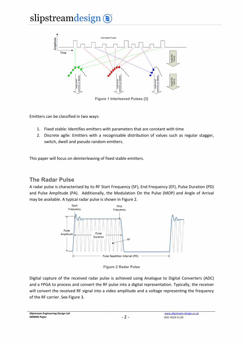
For the purpose of detecting and identifying radars in the environment, the pulse sequencesreceived from radars are used. The problem of determining the presence of a specific emitter in theenvironment is a problem of detecting a consistent pulse sequence in the incoming stream ofinterleaved pulses. Pulses arrive at the receiver of the system in natural time order and so becomeinterleaved as shown in Figure 1. Challenges exist when two or more emitters’ pulses overlap in timeand cannot be easily detected or are simply not received. This further increases the challenge ofdeinterleaving the pulses into identified emitters.

Conditions that have an impact on pulse train deinterleaving are [4]:· Pulse overlap,· Dropped pulses,· Extraneous pulses (multipath),· Intermittent pulse trains (effect of radar’s scan characteristic),· Pulse shadowing,· Receiver blanking.



Figure 1 Interleaved Pulses [3]

Emitters can be classified in two ways:

1. Fixed stable: Identifies emitters with parameters that are constant with time2. Discrete agile: Emitters with a recognisable distribution of values such as regular stagger,

switch, dwell and pseudo random emitters.

This paper will focus on deinterleaving of fixed stable emitters.

The Radar PulseA radar pulse is characterised by its RF Start Frequency (SF), End Frequency (EF), Pulse Duration (PD)and Pulse Amplitude (PA). Additionally, the Modulation On the Pulse (MOP) and Angle of Arrivalmay be available. A typical radar pulse is shown in Figure 2.

Figure 2 Radar Pulse

Digital capture of the received radar pulse is achieved using Analogue to Digital Converters (ADC)and a FPGA to process and convert the RF pulse into a digital representation. Typically, the receiverwill convert the received RF signal into a video amplitude and a voltage representing the frequencyof the RF carrier. See Figure 3.



Figure 3 Digital Capture system of Radar Pulse

The digital signal processing in the FPGA converts the received analogue pulse into a digital streamof pulse descriptor words (PDW). The pulse descriptor word includes the characterised pulseinformation with an applied time stamp (TS) of when the pulse arrived (TOA) in the system. Each oneof the parameters will be in the region of 16 to 31 data bits. These parameters are typicallyconverted into compensated and normalised parameters in their respective units, e.g frequency inMHz, Pulse Duration in us. Figure 4 shows a five parameter PDW.

Figure 4 Pulse Descriptor Word (PDW)

The deinterleaver may reside in either the FPGA, embedded system or industrial computerdepending on system requirements.

The transfer speed and volume of PDW’s between each of the systems on the data link requirescareful consideration. By way of an example, a system with a PDW of 160 bits in length, transferringon a serial link with a pulse duration of 50ns at 80% duty cycle requires 2.5Gbps, see Figure 5. Thepressure on the link will further increase with denser environments and multiple frequency bandinputs.

Figure 5 Data Saturation Point of Link

0.000

1.000

2.000

3.000

4.000

5.000

6.000

0 100 200 300 400 500 600

Syst

em B

andw

idth

(Gbp

s)

Pulse Width (ns)

Data Saturation Point (if duty-cycle is 80%)



ClusteringClustering is the technique of grouping together radar pulses into unique sets of emittercharacteristics using captured radar pulses and derived pulse characteristics such as Pulse RepetitionInterval (PRI). Clustering algorithms need to take into account known schemes applied to the pulsetrain by radar emitters such as:

1. Fixed stable – identifies emitters with values that are constant,2. Discrete agile – identifies emitters with a recognisable distribution of values such as regular

stagger, switch, dwell, wobulated (varying parameters in a wobble like fashion) and pseudorandom emitters.

It is important to consider the requirements of the overall system in terms of processing time andthe type of radar schemes that are expected to be present in the operational environment. Forexample, radar pulse deinterleaving of commercial marine ship radar’s characteristics maypredominately be expected to be constant, as opposed to a system required to cluster militaryradar’s which apply more complex agile schemes.

Not all parameters are useful in the initial deinterleaving and clustering of emitters. For example,pulse amplitude would not be used due to its varying nature. Frequency, pulse duration andmodulation of the pulse are the dominant parameters that can be used in the clustering process.

Clustering algorithmThe success of clustering is a balance between system performance requirements and cost. Sometechniques for clustering algorithms are described below in Table 1 for comparison. The remainderof this paper will be concerned with an improved version of the chain algorithm.

Technique OverviewChain Algorithm The algorithm calculates the difference Quick processing for fixed

between a sample pulse and an existing stable emitterscluster center of pulses. The cluster thatyields the smallest difference to thesample pulse and meets a requiredthreshold level is the closest match andthe sample pulse is added to the cluster.If the distance between the sample pulseand cluster is large a new cluster center iscreated.

Sequence Search By assuming a starting PRI estimation, the Quick processing for fixedMethod algorithm starts from the the first pulse in stable emitters

the buffer and then searches for the nextpulse, using the TOA the PRI can bederived from the two pulses.



The algorithm then searches through theremaining PDW data set searching for thenext pulse with that PRI. The algorithm isdesigned to manage missing pulsesthough the search. On completion ordetection of a large gap in the PDW datathe algorithm will stop and if enoughpulses exist for the PRI, mark and removethem from the data block. On completionof this, the algorithm resets to the firstpulse and continues to look for the nextvalid pulse and its PRI, the algorithmcontinues until all data is processed.

Histogram based Generally uses DTOA (Difference Time OfArrival) to determine PRI histograms.

As new emitters appear, peaks appear inthe PRI histogram identifying emitters.

PDW’s would usually be processed inblocks.

Time gaps in pulse streams can lead toincreased differences, causinguncertainty.

Various approaches can be used such as:· All difference Histogram· Difference Histogram· Sequential Difference Histogram· Cumulative Difference Histogram

Better performance on agileemitters.

Wavelet detectorMethod

Using a wavelet transform [1][2] usesTOA of the pulse. The approach is todetect if a signal with a period (T) at agiven time (t). If the detector exceeds athreshold a pulse train at a period (T) isfound.

Complexity can arise when multiplepoints exceed the threshold, this ishandled using decision making algorithmsand merging techniques.

Good for agile emitters

Table 1 Clustering Techniques



Chain Clustering AlgorithmIn order to cluster radar pulses, a distance clustering algorithm is required. This scheme determinesthe distance metric between two points (pulses) in a plane. The Euclidian distance function is usedand is given by:

��̅� , ��̅� = ��

�

��

Equation 1 Euclidian distance function

where �̅� and ��̅ are the distance of the pulses being measured and ��, �� are the�� feature of �̅�and ��̅ .

Modified Distance Function Applied to Radar PulseThe main objective is to determine if two pulses are similar to each other. This can be achieved byexpanding on the Euclidian to include PDW parameters of the radar pulse, Start Frequency (SF), EndFrequency (EF) and Pulse Duration (PD), see Equation 2. If further parameters are available, such asangle of arrival (AOA) and pulse modulation, these may be included in the algorithm. A weightingparameter is further added to the function that allows a weight for each of the pulse parameters.

�(�̅�� , �̅��) = ��|��|�

��

�

��

� + ��|��|�

��

�

��

� + ��|��|�

��

�

��

�

Equation 2 Expanded Distance Function

Where �̅�� is the first pulse or mean value of an accumulated clustered pulse set and �̅�� is thepulse to be used to measure the distance with.

The ClusterThe objective of the cluster is to hold received pulse descriptor words that are statistically similarand as such have a high probability of being from the same emitter type. The cluster may containmany unique emitters of the same type of radar system. At a later stage, unique emitters can beidentified using TOA, PRI, Amplitude, beam shapes and widths.



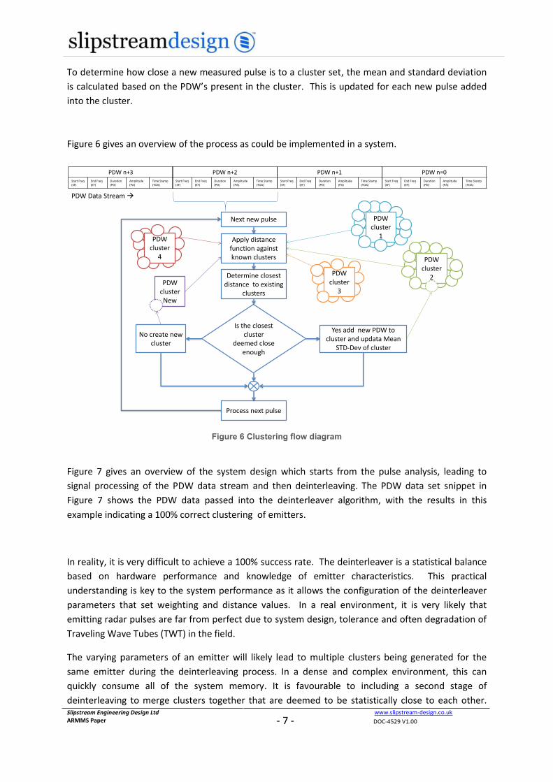
To determine how close a new measured pulse is to a cluster set, the mean and standard deviationis calculated based on the PDW’s present in the cluster. This is updated for each new pulse addedinto the cluster.

Figure 6 gives an overview of the process as could be implemented in a system.

Figure 6 Clustering flow diagram

Figure 7 gives an overview of the system design which starts from the pulse analysis, leading tosignal processing of the PDW data stream and then deinterleaving. The PDW data set snippet inFigure 7 shows the PDW data passed into the deinterleaver algorithm, with the results in thisexample indicating a 100% correct clustering of emitters.

In reality, it is very difficult to achieve a 100% success rate. The deinterleaver is a statistical balancebased on hardware performance and knowledge of emitter characteristics. This practicalunderstanding is key to the system performance as it allows the configuration of the deinterleaverparameters that set weighting and distance values. In a real environment, it is very likely thatemitting radar pulses are far from perfect due to system design, tolerance and often degradation ofTraveling Wave Tubes (TWT) in the field.

The varying parameters of an emitter will likely lead to multiple clusters being generated for thesame emitter during the deinterleaving process. In a dense and complex environment, this canquickly consume all of the system memory. It is favourable to including a second stage ofdeinterleaving to merge clusters together that are deemed to be statistically close to each other.

PDW n+2Start Freq(SF)

End Freq(EF)

Duration(PD)

Amplitude(PA)

Time Stamp(TOA)


End Freq(EF)

Duration(PD)

Amplitude(PA)

Time Stamp(TOA)

PDW n=0Start Freq(SF)

End Freq(EF)

Duration(PD)

Amplitude(PA)

Time Stamp(TOA)

PDWcluster

2

PDWcluster

1Apply distancefunction againstknown clusters

Next new pulse

Determine closestdistance to existing

clustersPDW

clusterNew

Yes add new PDW tocluster and updata Mean

STD-Dev of cluster

Is the closestcluster

deemed closeenough

Process next pulse

PDWcluster

3


End Freq(EF)

Duration(PD)

Amplitude(PA)

Time Stamp(TOA)

PDW Data Streamà

No create newcluster

PDWcluster

4



This approach allows system memory reuse and single emitters types to be merged together in amore efficient manner.

On completion of the deinterleaving process, the next stage would be to carry out emitteridentification within each of the cluster sets, using TDOA, sweep rates and beam width techniques tofurther extract emitters. Depending on the system, identified emitters can be placed in a clusterdatabase to improve system performance over time.

Figure 7 Clustering system

Real World DataThe radar environment can quickly become complex when there are a number of emitters present.Figure 8 presents a 2 second data capture. It is the deinterleavers task to make sense of this complexenvironment and present it in a usable format.

DigitalSignal

Processing

RF Pulse RF Characterised PDW Data Stream

PDW Data Set De-Interleaved Clusters Identified



Figure 8 Example radar data captures

Figure 9 shows the pulse descriptor word and the allocated cluster ID plotted against frequency andpulse duration. These results were obtained from the clustering algorithm described earlier runningon a small embedded system. (Red markers = SF, Blue markers = EF)

The successful clustering of emitters can clearly be seen with around 120 clusters generated for thisdataset.

In Figure 9, marker ‘A’ effectively shows a pulse cluster with different start and stop frequencies, andmarker ‘B’ shows a cluster with very few pulses.

Figure 10 is the same data but looking at 10 emitters in more detail. It can be observed that goodgrouping of the cluster parameters is achieved for these clusters.

Figure 11 shows the complexity of 120 emitters in the environment. This indicates a large number ofemitters operating at around 50-100ns pulse duration.



Figure 9 Example Clustering of Emitters

Figure 10 Clustered 10 Emitters Plotted against PD and Frequency

A

B



Figure 11 Clustered 120 Emitters Plotted against PD and Frequency

ConclusionGiven that the real world environment of radar pulses is very complex and taking into accountmillions of radar pulses and multipath effects, the improved chain sequence example explained inthe paper can be a good choice for systems deinterleaving fixed static emitters. The radar emitterenvironment soon get very complex in dense emitter environments and as such, a successful pulsedeinterleaver has a tough job.

Document References1 Ken’ichi Nishiguchi, “Time-period Analysis for Pulse Train Deinterleaving”

2 Douglas E. Driscoll & Stephen D. Howard, “THE DETECTION OF RADAR PULSE SEQUENCES BYMEANS OF A CONTINUOUS WAVELET TRANSFORM”, Electronic Warfare Division DefenceScience and Technology Organisation PO Box 1500, Salisbury, SA 5108, Australia

3 Pushparaj Silva, “Analyzing Tool for Radar Data”, ISSN-1653-5715

4 Rogers, J. A. V, “ESM Processor System for High Pulse Density Radar Environments”, IEEProceedings

Documents

8 - WIlson - It's a Complex World Radar Deinterleaving · IT’S€A€COMPLEX€WORLD€‘RADAR ... [email protected] Abstract ... as opposed to a system required