Embed Size (px)
Citation preview

Dr. Robert A. Schowengerdt, [email protected], 520-621-2706 (voice), -8076 (fax) 319 2003
MULTISPECTRAL CLASSIFICATION
DEFINITIONS

Dr. Robert A. Schowengerdt, [email protected], 520-621-2706 (voice), -8076 (fax) 320 2003
MULTISPECTRAL CLASSIFICATION
• Thematic maps
Informational description of a given area
Symbolic labels at each pixel replace numeric DNs in images
• Themes
For example: soil, water, vegetation
Desire direct relation between themes and geophysical variables, but a strong connection does not always exist
Also commonly called classes
• Physical Models
Explain some within-class variation in “signatures,” e.g. due to topographic shading
Remaining variation attributed to
• natural variation in signatures
• spectral mixing within GIFOV

Dr. Robert A. Schowengerdt, [email protected], 520-621-2706 (voice), -8076 (fax) 321 2003
MULTISPECTRAL CLASSIFICATION
THE CLASSIFICATION PROCESS
Feature Extraction
• Example features
original multispectral bands
subset of bands
derived features
• principal components
• vegetation indexes
• spatial properties
• Good features help to suppress or correct for known physical sources of variation
For example, multispectral ratios can reduce topographic shading

Dr. Robert A. Schowengerdt, [email protected], 520-621-2706 (voice), -8076 (fax) 322 2003
MULTISPECTRAL CLASSIFICATION
Data flow in classification
a
b
c
featureextraction
extracttraining pixels discriminant
functions
labeling
a
b
c
K-D feature space
multispectralimage
featureimage
thematicmap
training
determine
classifier
scene
sensoratmosphere

Dr. Robert A. Schowengerdt, [email protected], 520-621-2706 (voice), -8076 (fax) 323 2003
MULTISPECTRAL CLASSIFICATION
• Feature space
Because of class variability, the “signature” is actually a statistical distribution of feature vectors
Successful classification requires separated distributions, i.e. minimal overlap
Example with 2-D feature space, e.g. two bands of a multispectral image:
high separability low separability
possible classifierdecision boundaries
feature 1
feature 2

Dr. Robert A. Schowengerdt, [email protected], 520-621-2706 (voice), -8076 (fax) 324 2003
MULTISPECTRAL CLASSIFICATION
The Importance of Image Scale and Resolution
• Different classes require different sensor GIFOVs for identification
For example, man-made categories (streets, buildings, etc) require GIFOVs of 10m or less
Sea surface temperature, or global NDVI, can be measured sufficiently with larger GIFOVs, such as 1km
• Themes are often organized into a hierarchy
Higher levels in the hierarchy generally require higher resolution (smaller GIFOVs)
Different classes and hierarchies can be defined for different applications

Dr. Robert A. Schowengerdt, [email protected], 520-621-2706 (voice), -8076 (fax) 325 2003
MULTISPECTRAL CLASSIFICATION
Anderson land-use and land-cover labeling scheme for Levels I and II
Level I Level II
1 urban/built-up land 11 residential12 commercial and services13 industrial14 transportation, communication, and utili-ties
15 industrial and commercial complexes16 mixed urban/built-up land17 other urban/built-up land
2 agricultural land 21 cropland and pasture22 orchards, groves, vineyards, nurseries and ornamental horticultural areas
23 confined feeding operations24 other agricultural land
3 rangeland 31 herbaceous rangeland32 shrub and brush rangeland
23 mixed rangeland
4 forest land 41 deciduous forest land42 evergreen forest land
43 mixed forest land
5 water 51 streams and canals52 lakes
53 reservoirs54 bays and estuaries
6 wetland 61 forested wetland62 non-forested wetland
7 barren land 71 dry salt flats72 beaches73 sandy areas other than beaches74 bare exposed rock
75 strip mines, quarries, and gravel pits76 transitional areas77 mixed barren land
8 tundra 81 shrub and brush tundra82 herbaceous tundra83 bare ground tundra
84 wet tundra85 mixed tundra
9 perennial snow or ice 91 perennial snowfields 92 glaciers

Dr. Robert A. Schowengerdt, [email protected], 520-621-2706 (voice), -8076 (fax) 326 2003
MULTISPECTRAL CLASSIFICATION
Anderson land-use and land-cover labeling scheme for Level III
Level II Level III
11 residential 111 single family units112 multifamily units113 group quarters114 residential hotels115 mobile home parks116 transient lodgings117 other

Dr. Robert A. Schowengerdt, [email protected], 520-621-2706 (voice), -8076 (fax) 327 2003
MULTISPECTRAL CLASSIFICATION
CLASSIFICATION

Dr. Robert A. Schowengerdt, [email protected], 520-621-2706 (voice), -8076 (fax) 328 2003
MULTISPECTRAL CLASSIFICATION
Hard Versus Soft Classification
• Labeling of pixels accomplished by partitioning the feature space
• Hard classification results in one class/pixel
• Soft classification results in multiple classes/pixel, with associated likelihoods for each class:
"probabilities"parametric statistical classifiers
"membership grades"fuzzy classifiers
"fractions"mixture analysis
• Soft classification is more descriptive of reality
Accomodates within- and between-class variation
Accomodates class mixing within GIFOV

Dr. Robert A. Schowengerdt, [email protected], 520-621-2706 (voice), -8076 (fax) 329 2003
MULTISPECTRAL CLASSIFICATION
Visualization of hard versus soft classification
a
b
c
K-dimensionalfeature space
a
b
c
a
b
c
a,b,c
thematic mapmultispectral image
hard classification
soft classification

Dr. Robert A. Schowengerdt, [email protected], 520-621-2706 (voice), -8076 (fax) 330 2003
MULTISPECTRAL CLASSIFICATION
Supervised and Unsupervised Training
• Must "teach" the classifier algorithm to recognize the classes of interest
• Use sample pixels to represent the classes (“prototypes,” “exemplars,” or “training samples”)
• Training
derive features from sample pixels to determine decision boundaries between classes, according to the selected classification criteria

Dr. Robert A. Schowengerdt, [email protected], 520-621-2706 (voice), -8076 (fax) 331 2003
MULTISPECTRAL CLASSIFICATION
Supervised Training
• Training samples are labeled
Ground truth
Interpretation of higher resolution imagery (e.g. aerial photography)
Existing maps
• Identifying training sites (pixel samples) for each class can be laborious
Desire class-homogeneous sites, without mixture among classes
Also desire representation of full within-class variability
Therefore, often need more than one site/class
Some classes may have small spatial extent, e.g. “asphalt” roads

Dr. Robert A. Schowengerdt, [email protected], 520-621-2706 (voice), -8076 (fax) 332 2003
MULTISPECTRAL CLASSIFICATION
• Separability analysis
Useful for pre-classification analysis of supervised class signatures
Desire some measure of interclass similarity (or dissimilarity)
3 similarity measures based on class means
DN1
DN3
DN2
L1
L2
ANG
mb
ma

Dr. Robert A. Schowengerdt, [email protected], 520-621-2706 (voice), -8076 (fax) 333 2003
MULTISPECTRAL CLASSIFICATION
Similarity measures using class means only or class means and variances/covariances
name formula
city block
Euclidean
angular
normalized city block
Mahalanobis
L1 µa µb– mak mbk–
k 1=
K
∑= =
L2 µa µb– µa µb–( )T
µa µb–( )[ ]1 2⁄
= =
mak mbk–( )2
k 1=
K
∑1 2⁄
=
ANGµa
Tµb
µa µb----------------------
⎝ ⎠⎜ ⎟⎜ ⎟⎛ ⎞
acos=
NL1
mak mbk–
cak cbk+( ) 2⁄------------------------------------------
k 1=
K
∑=
MH µa µb–( )T Ca Cb+
2--------------------⎝ ⎠
⎛ ⎞1–
µa µb–( )1 2⁄
=

Dr. Robert A. Schowengerdt, [email protected], 520-621-2706 (voice), -8076 (fax) 334 2003
MULTISPECTRAL CLASSIFICATIONSeparability analysis can be used to find the best subset of features for given training data
• Calculate average separability among classes, using all possible combinations of k = 2 features, 3 features, etc. (k ≤ K)
• Choose the k features (out of K total features) that have highest separability for the given classes
• Can reduce computation load

Dr. Robert A. Schowengerdt, [email protected], 520-621-2706 (voice), -8076 (fax) 335 2003
MULTISPECTRAL CLASSIFICATIONUnsupervised Training
• Training samples are unlabeled
Sites need not be homogeneous, can use entire image if desired
• Algorithm used to find “natural” groupings of similar data, i.e. “clusters”
Resulting clusters are labeled by analyst using any available information (as in supervised training)
Clusters seldom are true concentrations of data, but just optimally-partitioned regions within feature space
• Data-driven, whereas supervised training is analyst-driven
Clustering can be helpful in finding homogeneous image areas for supervised training sites

Dr. Robert A. Schowengerdt, [email protected], 520-621-2706 (voice), -8076 (fax) 336 2003
MULTISPECTRAL CLASSIFICATION• K-means clustering algorithm
Iterative procedure
Adjusts cluster partitioning such that mean-squared distance of training samples from cluster means is minimized
Example convergence criteria
• net mean migration < threshold
• (Eq. 9-1)
• number of pixels that change labels between iterations < threshold
∆µµµµ i( ) µµµµk i( ) µµµµk i 1–( )–
k 1=
K
∑=

Dr. Robert A. Schowengerdt, [email protected], 520-621-2706 (voice), -8076 (fax) 337 2003
MULTISPECTRAL CLASSIFICATIONISODATA algorithm
• adds automated merging of similar clusters and splitting of heterogenous clusters
K-Means Clustering
• Specify K initial cluster mean estimates (“seeds”)
Note: K is not the number of features)
• Partition feature space according to nearest-mean rule
• Calculate revised cluster mean estimates from partitioned data
• Repeat 2 and 3 until convergence criterion is met

Dr. Robert A. Schowengerdt, [email protected], 520-621-2706 (voice), -8076 (fax) 338 2003
MULTISPECTRAL CLASSIFICATIONSchematic of ISODATA behavior
a
b
c
Calculate revised cluster mean
after iteration 2 after iteration 3
DNm
DNn
a
b
c
a
bc
a
bc
a
bc
mean vector migration
Specify K initial cluster mean estimates (“seeds”)
estimates from partitioned data and partition feature space

Dr. Robert A. Schowengerdt, [email protected], 520-621-2706 (voice), -8076 (fax) 339 2003
MULTISPECTRAL CLASSIFICATIONnet mean migration versus iteration number
0
1
2
3
4
5
6
7
1 2 3 4 5 6
net m
ean
mig
ratio
n (D
N)
iteration

Dr. Robert A. Schowengerdt, [email protected], 520-621-2706 (voice), -8076 (fax) 340 2003
MULTISPECTRAL CLASSIFICATIONImage example
• Marana, AZ, TM data, bands 3 and 4
Color IR composite
darksoil
crop
light soil

Dr. Robert A. Schowengerdt, [email protected], 520-621-2706 (voice), -8076 (fax) 341 2003
MULTISPECTRAL CLASSIFICATIONunsupervised cluster maps for various values of K
K = 2 3
4 5
67

Dr. Robert A. Schowengerdt, [email protected], 520-621-2706 (voice), -8076 (fax) 342 2003
MULTISPECTRAL CLASSIFICATIONfeature space cluster mean locations corresponding to Fig. 9-8
K = 2 3
4 5
67
At least 6 clusters needed to “capture” vegetation class because it is a numerically small population

Dr. Robert A. Schowengerdt, [email protected], 520-621-2706 (voice), -8076 (fax) 343 2003
MULTISPECTRAL CLASSIFICATIONresidual magnitude image error maps corresponding to Fig. 9-8
K = 2 3
4 5
6 7
Error is greatly reduced for vegetation with 6 or more clusters

Dr. Robert A. Schowengerdt, [email protected], 520-621-2706 (voice), -8076 (fax) 344 2003
MULTISPECTRAL CLASSIFICATIONtotal residual magnitude error in cluster map
0
10
20
30
40
50
2 3 4 5 6 7
resi
dual
err
or (
DN
)
number of clusters
Error drops by 25% in going from 5 to 6 clusters

Dr. Robert A. Schowengerdt, [email protected], 520-621-2706 (voice), -8076 (fax) 345 2003
MULTISPECTRAL CLASSIFICATIONHybrid Supervised/Unsupervised Training
• Combines the benefits of both types of training
Hybrid Training
• Cluster the image into a large number of cluster classes (say 50 or more)
Insures that classes are separable
• Using ancillary data, supervise the labeling of the clusters
Many will be merged into single, labeled classes
Result is a labeled map of fewer classes
• Accept labeled map as final, or do supervised classification, using labeled training samples from cluster map

Dr. Robert A. Schowengerdt, [email protected], 520-621-2706 (voice), -8076 (fax) 346 2003
MULTISPECTRAL CLASSIFICATIONNONPARAMETRIC CLASSIFICATION

Dr. Robert A. Schowengerdt, [email protected], 520-621-2706 (voice), -8076 (fax) 347 2003
MULTISPECTRAL CLASSIFICATIONLevel-Slice Classifier
• No assumed statistical distribution for classes, i.e. nonparametric
• Robust to variation in class signatures
• Performance cannot be predicted or supported by statistical theory
• Simple and efficient

Dr. Robert A. Schowengerdt, [email protected], 520-621-2706 (voice), -8076 (fax) 348 2003
MULTISPECTRAL CLASSIFICATION• Includes outlier “unclassified” label
Level-Slice Classifier
• Define L “boxes” in K-D feature space, one for each class at class mean ± k times class standard deviation
some software allows interactive specification of box boundaries in feature space
• If pixel vector lies within one box, assign that label to pixel
• If pixel vector lies in two or more overlapping boxes, use "tie-breaking" scheme
nearest-mean rule
b
c
a
DNm
DNn
label c
label a
label b
b versus c conflict
a versus b conflict
Feature-space decision boundaries

Dr. Robert A. Schowengerdt, [email protected], 520-621-2706 (voice), -8076 (fax) 349 2003
MULTISPECTRAL CLASSIFICATIONArtificial Neural Network (ANN) Classifier
• Classifier is a connected structure of simple decision elements (processing nodes)
• Classification capability contained in connecting weights between nodes
• Train with an iterative, optimization algorithm
For given training sample input vector, calculate output classification vector
• supervised training
Attempt to minimize mean-squared error in output classification vector (desire 1 at class node of interest, 0 for all other class nodes) over all training data
• Three-layer network can form second-order (nonlinear) decision boundaries
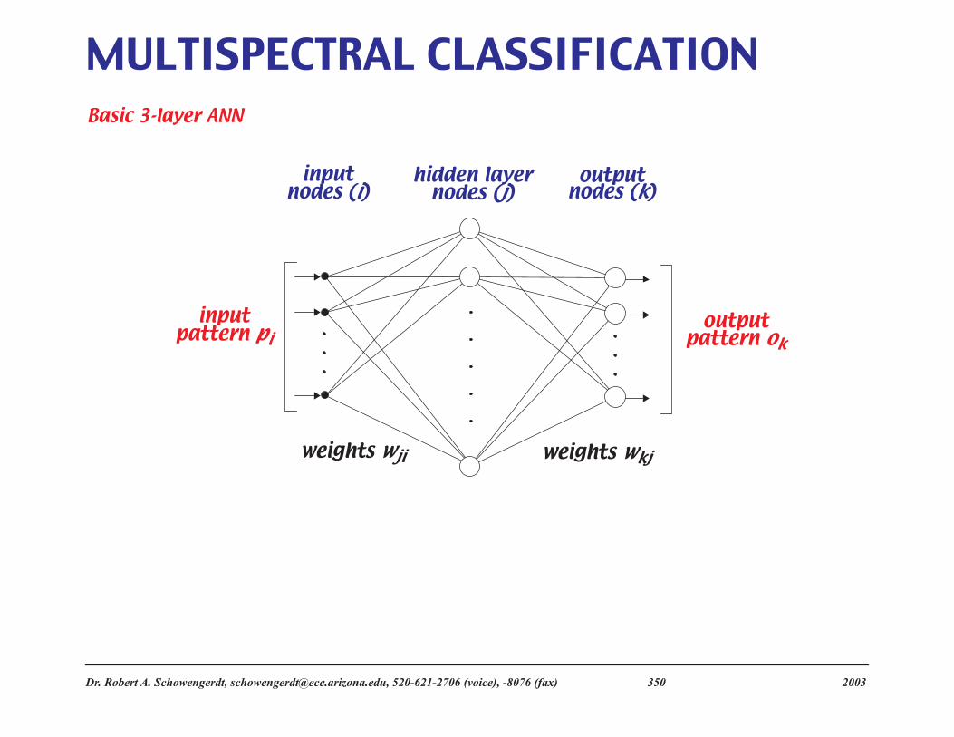
Dr. Robert A. Schowengerdt, [email protected], 520-621-2706 (voice), -8076 (fax) 350 2003
MULTISPECTRAL CLASSIFICATIONBasic 3-layer ANN
inputnodes (i)
hidden layernodes (j)
outputnodes (k)
weights wji weights wkj
inputpattern pi
outputpattern ok

Dr. Robert A. Schowengerdt, [email protected], 520-621-2706 (voice), -8076 (fax) 351 2003
MULTISPECTRAL CLASSIFICATION• Processing Nodes
Sums all the weighted inputs and passes the sum through a soft decision function (threshold)
Components of a processing node
typically, the decision function is a sigmoid function
(Eq. 9-4)
∑nodeinputs node output
activationfunction
Sf(S)
f S( ) 1
1 eS–
+-----------------=

Dr. Robert A. Schowengerdt, [email protected], 520-621-2706 (voice), -8076 (fax) 352 2003
MULTISPECTRAL CLASSIFICATIONSigmoid function
The threshold is usually “soft,” as above, but a “hard” threshold performs similarly
At each hidden layer node j, the input signals are weighted and summed, and then passed through the decision function
(Eq. 9-2)
at each output layer node k, the signals from the hidden layer nodes are weighted and summed, and then passed through the decision function
(Eq. 9-3)
0
0.25
0.5
0.75
1
-6 -4 -2 0 2 4 6
f(S)
S
Sj wjipii
∑=
hj f Sj( ) f wjipii
∑⎝ ⎠⎛ ⎞= =
Sk wkjhjj
∑=
ok f Sk( ) f wkjhjj
∑⎝ ⎠⎛ ⎞= =
f wkj wjipii
∑j
∑⎝ ⎠⎛ ⎞=

Dr. Robert A. Schowengerdt, [email protected], 520-621-2706 (voice), -8076 (fax) 353 2003
MULTISPECTRAL CLASSIFICATION• Back-Propagation Algorithm
Training algorithm to find “optimal” weights for the given training data
Member of iterative, gradient–descent family of algorithms
Steps
• 1. select training pixels for each class and specify desired output vector dk for class k (typically
dm=k = 0.9 and dm≠k = 0.1)
• 2. initialize weights as random numbers between 0 and 1 (typically small ≅ 0)
• 3. specify one training cycle:
• after each training pixel (sequential)
• after all training pixels in each class or
• after all training pixels in all classes (batch)
• 4. propagate training data forward through net, one pixel at a time
• 5. after each training cycle, calculate the output ok and the error relative to the desired output
dk, (the 1/2 factor is a mathematical convenience)

Dr. Robert A. Schowengerdt, [email protected], 520-621-2706 (voice), -8076 (fax) 354 2003
MULTISPECTRAL CLASSIFICATION
(Eq. 9-5)
• 6. adjust weight wkj by,
(Eq. 9-6)
where LR is the Learning Rate (controls speed of convergence)
• 7. adjust wji by
(Eq. 9-7)
• 8. do another training cycle (steps 4 through 7) until < threshold for all patterns (classes)
εεεε2
2---------- 1
2--- dk ok–( )
2
k∑
p 1=
P
∑=
∆wkj LR dk ok–( )Sd
d f S( )Sk
hjp 1=
P
∑=
∆wji LRSd
d f S( )Sj
dk ok–( )Sd
d f S( )Sk
wkj pik∑
⎩ ⎭⎨ ⎬⎧ ⎫
p 1=
P
∑=
ε

Dr. Robert A. Schowengerdt, [email protected], 520-621-2706 (voice), -8076 (fax) 355 2003
MULTISPECTRAL CLASSIFICATIONNonparametric Classification Examples
• Level-slice
Example level-slice classification
DN4
DN3
thematic map DN feature space
crop
light soil
dark soil

Dr. Robert A. Schowengerdt, [email protected], 520-621-2706 (voice), -8076 (fax) 356 2003
MULTISPECTRAL CLASSIFICATION• Artificial neural network
Convergence of the back-propagation algorithm
10-5
0.0001
0.001
0.01
0.1
0 500 1000 1500 2000 2500 3000
learning ratemomentum
valu
e
cycle
0.0001
0.001
0.01
0.1
1
0 500 1000 1500 2000 2500 3000
maximum errormean-squared errorou
tput
err
or
cycle

Dr. Robert A. Schowengerdt, [email protected], 520-621-2706 (voice), -8076 (fax) 357 2003
MULTISPECTRAL CLASSIFICATIONHard classification maps at three stages of iteration
cycle 250
cycle 500
cycle 1000
DN4
DN3
croplight soil
dark soil

Dr. Robert A. Schowengerdt, [email protected], 520-621-2706 (voice), -8076 (fax) 358 2003
MULTISPECTRAL CLASSIFICATIONFinal ANN hard classification map
DN4
DN3
thematic map DN feature space
crop
light soil
dark soil

Dr. Robert A. Schowengerdt, [email protected], 520-621-2706 (voice), -8076 (fax) 359 2003
MULTISPECTRAL CLASSIFICATIONSoft classification maps at four iterations crop light soildark soil
cycle 250
cycle 500
cycle 750
cycle 1000
All classes “build” over iterations
Small crop class takes longer to “build” than other classes
Dr. Robert A. Schowengerdt, [email protected], 520-621-2706 (voice), -8076 (fax) 360 2003
MULTISPECTRAL CLASSIFICATIONPARAMETRIC CLASSIFICATION

Dr. Robert A. Schowengerdt, [email protected], 520-621-2706 (voice), -8076 (fax) 361 2003
MULTISPECTRAL CLASSIFICATIONEstimation of Model Parameters
• Classifier depends on parameters of assumed class statistical distribution
• The class conditional probabilities, , for a feature vector f, are estimated from the training data for each class i
has unit area (unit volume in K-D)
• The a priori probabilities, , are estimated by the total percent coverage of each class
Usually set equal for all classes, i.e. . (unbiased)
• To perform a classification of non-training pixels, we need the a posteriori probabilities,
p f i⁄( )
p f i⁄( )
p j( )
1# classes---------------------
p i f⁄( )
Dr. Robert A. Schowengerdt, [email protected], 520-621-2706 (voice), -8076 (fax) 362 2003
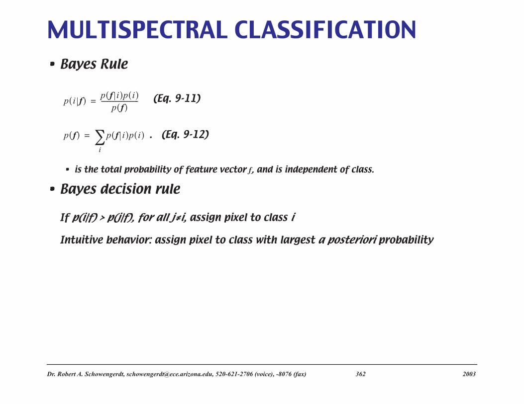
MULTISPECTRAL CLASSIFICATION• Bayes Rule
(Eq. 9-11)
. (Eq. 9-12)
• is the total probability of feature vector f, and is independent of class.
• Bayes decision rule
If p(i|f) > p(j|f), for all j≠i, assign pixel to class i
Intuitive behavior: assign pixel to class with largest a posteriori probability
p i f( )p f i( )p i( )
p f( )------------------------=
p f( ) p f i( )p i( )
i∑=

Dr. Robert A. Schowengerdt, [email protected], 520-621-2706 (voice), -8076 (fax) 363 2003
MULTISPECTRAL CLASSIFICATIONDiscriminant Functions
• Restate Bayes decision rule
If , for all j≠i, assign pixel to class i
where the discrimant function for class i, , is given by,
(Eq. 9-13)
• Any monotonic function of p(i|f)p(f), also works as a discriminant function
For example (Eq. 9-14)
or (Eq. 9-15)
The log transformation in Eq. 9-15 is advantageous for normal distributions
Di f( ) Dj f( )>
Di f( )
Di f( ) p i f( )p f( ) p f i( )p i( ).= =
Di f( ) Ap i f( )p f( ) B+ Ap f i( )p i( ) B+= =
Di f( ) p i f( )p f( )[ ]ln p f i( )p i( )[ ]ln= =

Dr. Robert A. Schowengerdt, [email protected], 520-621-2706 (voice), -8076 (fax) 364 2003
MULTISPECTRAL CLASSIFICATIONThe Normal Distribution Model
• Common statistical assumption
Note, Bayes decision rule does not require normal distributions
Little research or data on normality of training pixels in remote sensing data
• Assuming normal (Gaussian) distribution in K-D
(Eq. 4-18)
and Eq. 9-15,
(Eq. 9-16)
Only the last term needs to be recalculated at each pixel
N DN µµµµ; C,( ) 1
C1 2⁄
2π( )K 2⁄
-------------------------------------eDN µµµµ–( )– TC 1– DN µµµµ–( ) 2⁄
=
Di f( ) p i( )[ ]ln 12--- K 2π[ ]ln Ciln f µi–( )
TCi
1–f µi–( )+ +
⎩ ⎭⎨ ⎬⎧ ⎫
–=

Dr. Robert A. Schowengerdt, [email protected], 520-621-2706 (voice), -8076 (fax) 365 2003
MULTISPECTRAL CLASSIFICATIONDecision boundaries (Gaussian PDF)
• located where the probabilities of classes are equal
• quadratics in 2-D and hyperquadrics in K-D
• The decision rule is equivalent to setting, for two classes a and b,
or (Eq. 9-18)p a f( )p f( )[ ]ln p b f( )p f( )[ ]ln= p a f( ) p b f( )=
-100
-80
-60
-40
-20
0
0 10 20 30 40 50 60 70 80
class aclass bln
[p(i
|DN
)p(D
N)]
DN
0
0.02
0.04
0.06
0.08
0.1
0.12
0 10 20 30 40 50 60 70 80
class a
class b
p(i|D
N)p
(DN
)
DN
label blabel a label a
discriminant functionsa posteriori probabilities
label blabel a label a

Dr. Robert A. Schowengerdt, [email protected], 520-621-2706 (voice), -8076 (fax) 366 2003
MULTISPECTRAL CLASSIFICATIONMaximum-likelihood classifier
• Minimizes total misclassification error,
where is the error that a pixel belonging to class j is mislabeled as class i
εtotal ε i j( )all i j≠
∑=
ε i j( )
Quadratic decision boundaries in 2-D feature space
c
b
c
a
DNm
DNn
label c
label a
label b

Dr. Robert A. Schowengerdt, [email protected], 520-621-2706 (voice), -8076 (fax) 367 2003
MULTISPECTRAL CLASSIFICATION
Maximum-Likelihood Classifier
• Estimate mean vector mi and covariance matrix Ci for each
class from the DN mean and covariance of training data
• Calculate discriminant functions at each image pixel (Eq. 9-16)
• For each unlabeled pixel, assign the label of the class with the largest discriminant function (i.e. the largest a posteriori probability)

Dr. Robert A. Schowengerdt, [email protected], 520-621-2706 (voice), -8076 (fax) 368 2003
MULTISPECTRAL CLASSIFICATIONThe Nearest-Mean Classifier
• Special case of the maximum-likelihood classifier
• Also called minimum-Euclidean distance classifier
• Assumes
Class covariance matrices are equal and diagonal
(Eq. 9-23)
A priori probabilities are equal
C0
c0 … 0
: : 0 … c0
=

Dr. Robert A. Schowengerdt, [email protected], 520-621-2706 (voice), -8076 (fax) 369 2003
MULTISPECTRAL CLASSIFICATION• Discriminant function then
becomes
(Eq. 9-24)
which is (almost) the Euclidean distance of a pixel vector f from a class mean vector µι.
This discriminant function will be a maximum when the distance is a minimum (because of negative sign on the second term)
So, maximizing the discriminant function minimizes the Euclidean distance
Di f( ) Af µi–( )T
f µi–( )
2c0--------------------------------------–=
Linear decision boundaries in 2-D feature space
b
c
a
DNm
DNn
label c
label a
label b
Dr. Robert A. Schowengerdt, [email protected], 520-621-2706 (voice), -8076 (fax) 370 2003
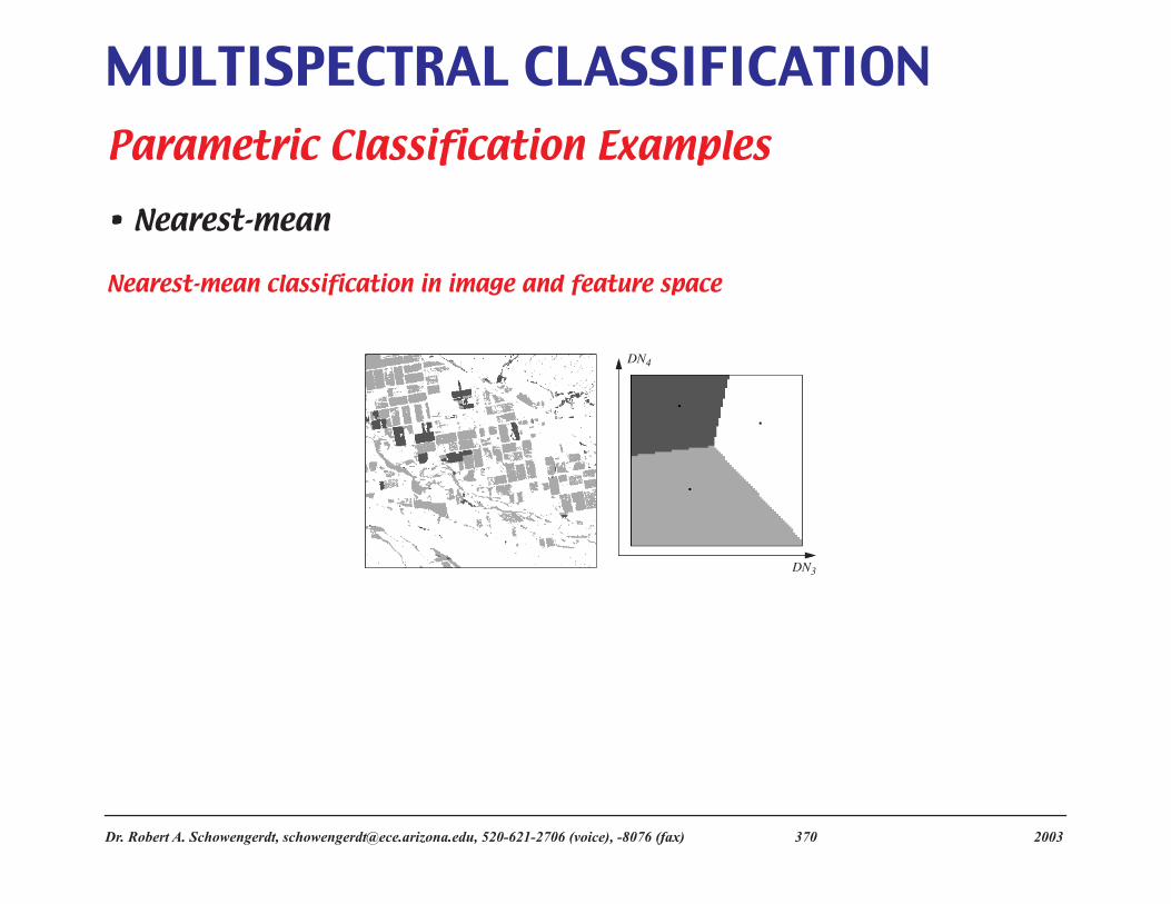
MULTISPECTRAL CLASSIFICATIONParametric Classification Examples
• Nearest-mean
Nearest-mean classification in image and feature space
DN4
DN3

Dr. Robert A. Schowengerdt, [email protected], 520-621-2706 (voice), -8076 (fax) 371 2003
MULTISPECTRAL CLASSIFICATION• Maximum-likelihood
Maximum-likelihood classification in image and feature space, without and with probability threshold
DN4
DN3T = 0%
T = 1%
DN4
DN3

Dr. Robert A. Schowengerdt, [email protected], 520-621-2706 (voice), -8076 (fax) 372 2003
MULTISPECTRAL CLASSIFICATIONModeling of class distributions with Gaussians
• Two-class example (Lake Anna, Virginia, MSS image)
Image with training sites

Dr. Robert A. Schowengerdt, [email protected], 520-621-2706 (voice), -8076 (fax) 373 2003
MULTISPECTRAL CLASSIFICATIONGaussian models compared to class distributions
0
0.1
0.2
0.3
0.4
0.5
0.6
0.7
0 5 10 15 20
water, site 1 histogram
water, site 1 gaussian model
prob
abil
ity
DN
0
0.01
0.02
0.03
0.04
0.05
0.06
0 20 40 60 80 100
vegetation histogram
vegetation gaussian model
prob
abil
ity
DN

Dr. Robert A. Schowengerdt, [email protected], 520-621-2706 (voice), -8076 (fax) 374 2003
MULTISPECTRAL CLASSIFICATIONClassifications with one training site/class
nearest-mean
maximum-likelihood

Dr. Robert A. Schowengerdt, [email protected], 520-621-2706 (voice), -8076 (fax) 375 2003
MULTISPECTRAL CLASSIFICATIONEffect of a priori probabilities on model fit
0
0.05
0.1
0.15
0.2
0.25
0 20 40 60 80 100
histogram (%)sum of gaussian models, equal priorssum of gaussian models, unequal priors
a po
ster
iori
pro
babi
lity
DN
N-MM-L

Dr. Robert A. Schowengerdt, [email protected], 520-621-2706 (voice), -8076 (fax) 376 2003
MULTISPECTRAL CLASSIFICATIONModel fit with 2 training sites for water
0
0.01
0.02
0.03
0.04
0.05
0.06
0 20 40 60 80 100
histogram (%)sum of gaussian models, unequal priors
a po
ster
iori
pro
babi
lity
DN
N-MM-L

Dr. Robert A. Schowengerdt, [email protected], 520-621-2706 (voice), -8076 (fax) 377 2003
MULTISPECTRAL CLASSIFICATIONFinal maximum-likelihood classification

Dr. Robert A. Schowengerdt, [email protected], 520-621-2706 (voice), -8076 (fax) 378 2003
MULTISPECTRAL CLASSIFICATIONSPATIAL-SPECTRAL SEGMENTATION

Dr. Robert A. Schowengerdt, [email protected], 520-621-2706 (voice), -8076 (fax) 379 2003
MULTISPECTRAL CLASSIFICATIONSpatial-Spectral Model
• neighboring pixels are likely to belong to same spectral class
• Goal is to group “connected” pixels into spatial segments
• May be thought of as “spatial clustering,” using a spectral similarity criterion
Region Growing
• Types of “connectedness”
4-connected
• only vertical and horizontal neighbors
8-connected
• all 8 neighbors, including diagonal neighbors

Dr. Robert A. Schowengerdt, [email protected], 520-621-2706 (voice), -8076 (fax) 380 2003
MULTISPECTRAL CLASSIFICATIONConnectedness definitions
4-connected 8-connected
3 x 3 pixel neighborhood
possible connected region

Dr. Robert A. Schowengerdt, [email protected], 520-621-2706 (voice), -8076 (fax) 381 2003
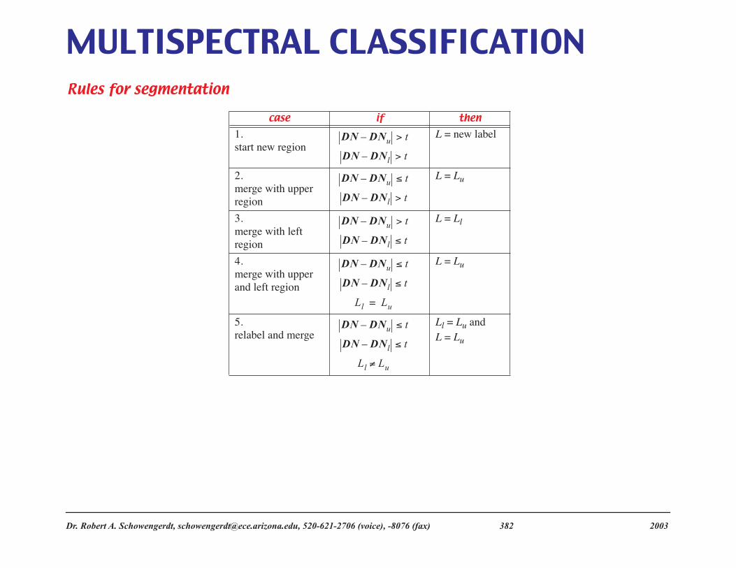
MULTISPECTRAL CLASSIFICATION4-connected region growing algorithm
• DN difference threshold t between a pixel and its neighbors
• Proceed top-to-bottom, left-to-right across image with 3-pixel window
Pixel and label windows
• Apply series of rules to test for connectivity at each pixel
DNu
DNl DN
Lu
Ll L
image label map
Dr. Robert A. Schowengerdt, [email protected], 520-621-2706 (voice), -8076 (fax) 382 2003
MULTISPECTRAL CLASSIFICATIONRules for segmentation
case if then
1.start new region
L = new label
2.merge with upper region
L = Lu
3.merge with left region
L = Ll
4.merge with upper and left region
L = Lu
5.relabel and merge
Ll = Lu andL = Lu
DN DNu– t>
DN DNl– t>
DN DNu– t≤
DN DNl– t>
DN DNu– t>
DN DNl– t≤
DN DNu– t≤
DN DNl– t≤
Ll Lu=
DN DNu– t≤
DN DNl– t≤
Ll Lu≠

Dr. Robert A. Schowengerdt, [email protected], 520-621-2706 (voice), -8076 (fax) 383 2003
MULTISPECTRAL CLASSIFICATION• Steps
1. Label first row of pixels
• assign L=0 at first pixel (upper left corner of image)
• use modified Cases 1 and 3 for remaining pixels in first row
2. Label first pixel, second row
• use modified Cases 1 and 3
3. Label remaining pixels in second row using all Cases 1 - 5 in Table 9-6.
modified case if then
1.start new region
L = new label
3.merge with left region
L = Ll
modified case if then
1.start new region
L = new label
3.merge with upper region
L = Lu
DN DNl– t>
DN DNl– t≤
DN DNu– t>
DN DNu– t≤

Dr. Robert A. Schowengerdt, [email protected], 520-621-2706 (voice), -8076 (fax) 384 2003
MULTISPECTRAL CLASSIFICATION4. Repeat steps 2 and 3 for remaining rows until finished
• Optional second pass can be done to merge similar regions
decide on merging two connected regions using threshold on the DN variance of the resulting combined region
• Final pass required to resequence labels

Dr. Robert A. Schowengerdt, [email protected], 520-621-2706 (voice), -8076 (fax) 385 2003
MULTISPECTRAL CLASSIFICATIONSignature maps for two thresholds
TM3 TM4
t = 2
t = 5
Larger t results in more aggregation and, therefore, fewer, but larger, regions

Dr. Robert A. Schowengerdt, [email protected], 520-621-2706 (voice), -8076 (fax) 386 2003
MULTISPECTRAL CLASSIFICATIONError maps between signature maps and image
t = 2 t = 5
Number of regions and DN error versus threshold
0
1 104
2 104
3 104
4 104
0
1
2
3
4
5
6
7
2 3 4 5 6 7 8 9 10 11
number of regions
average DN errornu
mbe
r of
reg
ions
DN difference threshold, t
average DN
error
• Convergence properties
Speed of convergence (as a function of threshold t) depends on image structure

Dr. Robert A. Schowengerdt, [email protected], 520-621-2706 (voice), -8076 (fax) 387 2003
MULTISPECTRAL CLASSIFICATION• Effect on multispectral feature space
Spatial segmentation causes “coalescing” of DN vectors into “clusters”
• Connected object regions in an image tend to consist of several or more pixels with similar spectral vectors
Can be a useful precursor to spectral clustering
• Disconnected regions with similar spectral vectors will have different labels from segmentation; such regions will be given the same label by clustering
• Adds spatial connectedness information to spectral similarity information

Dr. Robert A. Schowengerdt, [email protected], 520-621-2706 (voice), -8076 (fax) 388 2003
MULTISPECTRAL CLASSIFICATIONExample using TM (Marana, AZ) scattergram
2500
2000
1500
1000
500
0
0
500
1000
1500
2000
2500
2500
2000
1500
1000
500
0
0
500
1000
1500
2000
2500
DN3
DN4
DN4
DN3
original image segmented image (t = 5)

Dr. Robert A. Schowengerdt, [email protected], 520-621-2706 (voice), -8076 (fax) 389 2003
MULTISPECTRAL CLASSIFICATIONSUBPIXEL CLASSIFICATION

Dr. Robert A. Schowengerdt, [email protected], 520-621-2706 (voice), -8076 (fax) 390 2003
MULTISPECTRAL CLASSIFICATIONSpatial-Spectral Mixing
• Spatial integration within the sensor GIFOV
GIFOV = 1 x 1 3 x 3
7 x 7 13 x 13

Dr. Robert A. Schowengerdt, [email protected], 520-621-2706 (voice), -8076 (fax) 391 2003
MULTISPECTRAL CLASSIFICATION• Weighted spatial integration within net sensor spatial response
scene detector GIFOV effective net GIFOV

Dr. Robert A. Schowengerdt, [email protected], 520-621-2706 (voice), -8076 (fax) 392 2003
MULTISPECTRAL CLASSIFICATION• Simple geometric model for
spatial-spectral mixing
class a: 65% area, spectrum Ea
class b: 20% area, spectrum Eb
class c: 15% area, spectrum Ec
total spectrum at pixel: DN = 0.65Ea + 0.20Eb + 0.15Ec
one GIFOV:
b b
a
c
0
0.1
0.2
0.3
0.4
0.5
0.6
400 800 1200 1600 2000 2400
Kentucky Blue GrassDry Red Clay (5% water)50/50 mixture
refle
ctan
ce
wavelength (nm)

Dr. Robert A. Schowengerdt, [email protected], 520-621-2706 (voice), -8076 (fax) 393 2003
MULTISPECTRAL CLASSIFICATION• Linear mixing model based on proportions of the spectral
signatures within each pixel
Assumes the spectrum at each pixel can be represented by a linear combination of pure “end-member” spectra
• In vector-matrix form, for K bands and N end-members:
where
• is the K x 1 hyperspectral vector at pixel ij
• is the K x N end member spectrum matrix. Each column is the spectrum for one end-member
• is the N x 1 fraction vector of each end-member for pixel ij
• To find f at each pixel, we must invert the above equation.
DNij E f ij=
DNij
E
f ij

Dr. Robert A. Schowengerdt, [email protected], 520-621-2706 (voice), -8076 (fax) 394 2003
MULTISPECTRAL CLASSIFICATION• Since K >> N, inversion is a least-squares problem to find the
estimated fraction vector that minimizes the total error:
(Eq. 9-34)
• Use pseudoinverse solution, at each pixel:
(Eq. 9-33)
• Additional contraints:
(Eq. 9-26 and 9-27)
f̂ij
min εijT
εij[ ] DNij Ef̂ij–( )T
DNij Ef̂ij–( )=
f̂ij ET
E( )1–E
TDNij⋅=
f n 0 f nn 1=
N
∑ 1=,≥

Dr. Robert A. Schowengerdt, [email protected], 520-621-2706 (voice), -8076 (fax) 395 2003
MULTISPECTRAL CLASSIFICATION• Convex hull
Defined by outer boundary connecting end-members
Three possible endmember sets in 2-D
DN3
DN4
dark soil
light soil
crop

Dr. Robert A. Schowengerdt, [email protected], 520-621-2706 (voice), -8076 (fax) 396 2003
MULTISPECTRAL CLASSIFICATION• Ways to find the end–members
Laboratory or field reflectance spectra. Image data must be calibrated to reflectance.
Image pixels modeled as mixtures of library reflectance spectra. Image data must be calibrated to reflectance.
Automated techniques based on image transforms, e.g. PCT
K-dimensional interactive visualization tools

Dr. Robert A. Schowengerdt, [email protected], 520-621-2706 (voice), -8076 (fax) 397 2003
MULTISPECTRAL CLASSIFICATIONUnmixing example
• Two bands of TM image with three classes
• 2-D multispectral vector at each pixel,
, (Eq. 9-28)
or,
(Eq. 9-29)
which is underdetermined.
DNij Efij=
DN3
DN4
Edksoil3 Eltsoil3 Ecrop3
Edksoil4 Eltsoil4 Ecrop4
fdksoil
fltsoil
fcrop
=

Dr. Robert A. Schowengerdt, [email protected], 520-621-2706 (voice), -8076 (fax) 398 2003
MULTISPECTRAL CLASSIFICATION• Incorporate full coverage constraint at each pixel:
(Eq. 9-30)
• Augmented mixing equation
(Eq. 9-31)
• Solve exactly for class fractions
(9-32)
1 fdarksoil flightsoil fcrop+ +=
DN3
DN4
1
Edksoil3 Eltsoil3 Ecrop3
Edksoil4 Eltsoil4 Ecrop4
1 1 1
fdksoil
fltsoil
fcrop
=
fdksoil
fltsoil
fcrop
Edksoil3 Eltsoil3 Ecrop3
Edksoil4 Eltsoil4 Ecrop4
1 1 1
1–DN3
DN4
1
=

Dr. Robert A. Schowengerdt, [email protected], 520-621-2706 (voice), -8076 (fax) 399 2003
MULTISPECTRAL CLASSIFICATIONClass fraction maps produced for two different sets of end-members
dark soil
light soil
crop
data-defined endmembers “virtual” endmembers

Dr. Robert A. Schowengerdt, [email protected], 520-621-2706 (voice), -8076 (fax) 400 2003
MULTISPECTRAL CLASSIFICATIONEnd-member values for example
endmember type
band dark soil
light soil crop
data-defined 3 18 84 21
4 14 72 84
virtual 3 15 93 14
4 6 77 90

Dr. Robert A. Schowengerdt, [email protected], 520-621-2706 (voice), -8076 (fax) 401 2003
MULTISPECTRAL CLASSIFICATIONAlternate interpretations of mixing analysis
• Class fractions represent spectral mixing
“intimate” mixing caused by lack of one-to-one correspondance between class labels and spectral signatures
• Class fractions represent spatial mixing within GIFOV and spatial response function
Independent of spectral similarity of classes
• Other mixing indicators
output node values in a ANN classification
a posteriori probabilities in a maximum-likelihood classification

Dr. Robert A. Schowengerdt, [email protected], 520-621-2706 (voice), -8076 (fax) 402 2003
MULTISPECTRAL CLASSIFICATIONClassification Comparisons
• Soft image maps
TM CIR (bands 4, 3, 2)
ANN output
mixing fractions
Dr. Robert A. Schowengerdt, [email protected], 520-621-2706 (voice), -8076 (fax) 403 2003
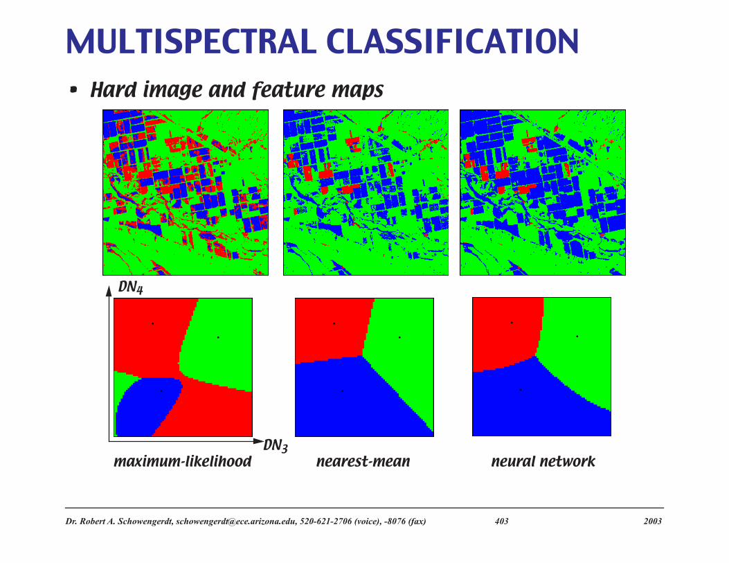
MULTISPECTRAL CLASSIFICATION• Hard image and feature maps
maximum-likelihood nearest-mean neural network
DN3
DN4

Dr. Robert A. Schowengerdt, [email protected], 520-621-2706 (voice), -8076 (fax) 404 2003
MULTISPECTRAL CLASSIFICATION


![In Rock [UA] – TRIBUTE: The Best of In Rock [UA]](https://img.pdfslide.us/doc/110x75/568bf0fe1a28ab893391a086/in-rock-ua-tribute-the-best-of-in-rock-ua.jpg)