Embed Size (px)
Citation preview
8-PSK SIGNALING OVER NON-LINEAR
SATELLITE CHANNELS
Ruben Caballero, B. ENG.
Dr. Sheila Horan
NMSU-ECE-96-010 May 1996

8-PSK SIGNALING
OVER NON-LINEAR
SATELLITE CHANNELS
BY
RUBI_N CABALLERO, B.ENG.
A Thesis submitted to the Graduate School
in partial fulfillment of the requirements
for the Degree
Master of Science in Electrical Engineering
New Mexico State University
Las Cruces, New Mexico
May 1996
ACKNOWLEDGMENTS
Throughout my young career as an engineer, I always had a particular feeling, that was well
expressed, by the French philosopher and mathematician Descartes in the 17 thcentury:
" ,_ la rue d'ing_nieuse d_couvertes, je me demandais sije ne pourrais pas
inventer par moi-m_me sans m 'appuyer sur la lecture d'un auteur... "
My two years of graduate study and this thesis allowed me to answer to this affmTtation.
First, I would like to thank Dr. Sheila Horan, my thesis advisor, for her help, direction and advice
toward the completion of my research. To Dr. Stephen Horan and Dr. William Ryan, I also wish to
give my thanks for sharing with me their engineering expertise and advice. I also would like to thank
Dr. James P. Reilly who served on my thesis committee and the students in the Center for Space
Telemetering and Telecommunications Systems in the Klipsch School of Electrical and Computer
Engineering Department for their dedication towards Telemetry and Space-Communications.
I am also deeply grateful to the Canadian Air Force and the Canadian Government for their support
in the completion of my Master's degree. I also thank NASA for their support under Grant # NAG
5-1491 and for giving me the chance to work on this project.
Finalmente, no existen suficientes palabras para describir el cafiflo y amor que le tengo a mi
familia, Los Caballero, sin quienes nunca habria llegado hasta donde hoy estoy. Muchisimas gracias a
mi padre, Luis, mi madre, Luz, y a mi dos hermanitas, Maria-Paz y Joanna Manuela.
iii
ABSTRACT
8-PSK SIGNALING
OVER NON-LINEAR
SATELLITE CHANNELS
BY
RUBt_N CABALLERO, B.ENG.
Master of Science in Electrical Engineering
New Mexico State University
Las Cruces, New Mexico, 1996
Dr. Sheila B. Horan, Chair
Space agencies are under pressure to utilize better bandwidth-efficient communication methods due
to the actual allocated frequency bands becoming more congested. Also budget reductions is another
problem that the space agencies must deal with. This budget constraint results in simpler spacecraft
carrying less communication capabilities and also the reduction in staff to capture data in the earth
stations. It is then imperative that the most bandwidth efficient communication methods be utilized.
This thesis presents a study of 8-ary Phase Shift Keying (8PSK) modulation with respect to
bandwidth, power efficiency, spurious emissions and interference susceptibility, over a non-linear
satellite channel.
Anend-to-endsystemperformance,includingtheInterSymboiInterference(ISI) andtheSymbol
ErrorRate(SER)asafunctionof Eb/Noon8PSKmodulationwasconductedonSignalProcessing
Worksystem(SPW)softwareinstalledonaSUNSpareStationl0 andaHewlettPackard(HP)Model
715/100UnixStation.ThesimulationswerebasedontheNon-Return-to-Zero(NRZ)dataformat.
Theend-to-end system evaluation was performed using idea! and non-ideal data with ideal system
components and three baseband filter types: 5th Order Butterworth, 3rd Order Bessel and Square Root
Raised Cosine (SRRC), ct = 0.25, 0.5 and 1, to observe the effect of pulse shaping on bandwidth and
SER.
The simulations show that in-band spurious emissions are greater in number and more evident for
the Bessel Filter than the Burterworth Filter with a Bandwidth (3dB)-Time product equal to I (BT=I).
With respect to the sideband attenuation, it was found that the values of attenuation for the 3rd Order
Bessel filter are comparable to the 5th Order Butterworth filter. For SRRC filters with ct = 0.25 and
ct = 0.5, the bandwidth is narrower than the Butterworth and Bessel Filters, but the attenuation is less
at high frequencies. Nonetheless, the absence of spurious emissions is a net advantage. For SRRC
ct = 1, the bandwidth is wider than the two previous SRRC filters and the absence of in-band spurious
emissions was again noticed. Less sideband attenuation was recorded for this roll-off factor compared
with a = 0.25 and ct = 0.5. For SER, it was found that the Butterworth and Bessel Filters just barely
meet the threshold of ISI loss < 0.4 dB at SER = 10-3 . Also the SRRC filters do not meet this
specification. From these results, it can be stipulated that the 5 th Order Butterworth filter has a small
advantage compared to the other filters. Overall, it was shown by using baseband filtering that the
bandwidth utilization can be improved by a factor of 12 to 24 with BT=I and 8PSK which can
significantly increase the spectrum utilization. Also a study on the tradeoffs between non-constant
envelope and bandwidth in a non-linear system, Solid State Power Amplifier (SSPA), is discussed.
vi
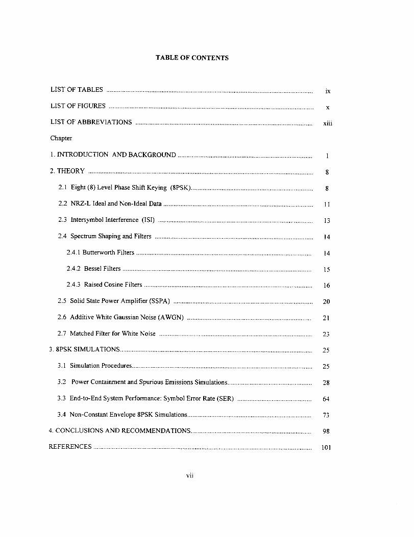
TABLE OF CONTENTS
LIST OF TABLES ........................................................................................................................ ix
LIST OF FIGURES ....................................................................................................................... x
LIST OF ABBREVIATIONS ....................................................................................................... xiii
Chapter
1. INTRODUCTION AND BACKGROUND .............................................................................. 1
2. THEORY ................................................................................................................................... 8
2.1 Eight (8) Level Phase Shift Keying (8PSK) ....................................................................... 8
2.2 NRZ-L Ideal and Non-Ideal Data ....................................................................................... 11
2.3 lntersymbol Interference (ISI) .......................................................................................... 13
2.4 Spectrum Shaping and Filters ............................................................................................ 14
2.4.1 Burterworth Filters ...................................................................................................... 14
2.4.2 Bessel Filters .............................................................................................................. 15
2.4.3 Raised Cosine Filters .................................................................................................. 16
2.5 Solid State Power Amplifier (SSPA) ................................................................................. 20
2.6 Additive White Gaussian Noise (AWGN) ........................................................................ 21
2.7 Matched Filter for White Noise ......................................................................................... 23
3.8PSK SIMULATIONS ................................................................................................................ 25
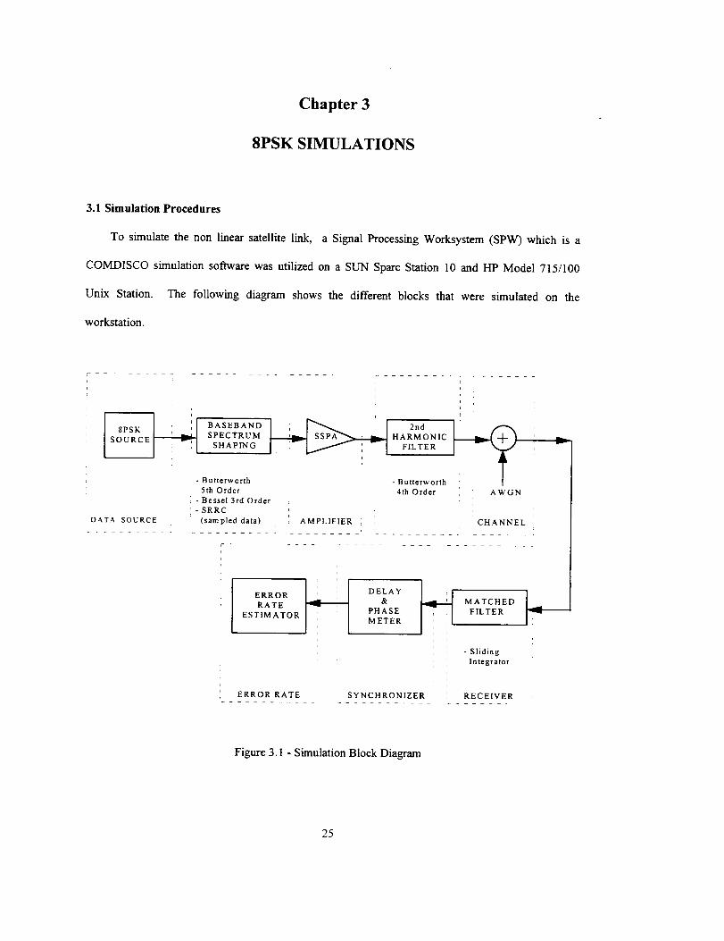
3.1 Simulation Procedures ......................................................................................................... 25
3.2 Power Containment and Spurious Emissions Simulations ................................................. 28
3.3 End-to-End System Performance: Symbol Error Rate (SER) ........................................... 64
3.4 Non-Constant Envelope 8PSK Simulations ........................................................................ 73
4. CONCLUSIONS AND RECOMMENDATIONS ...................................................................... 98
REFERENCES ............................................................................................................................... 101
vii
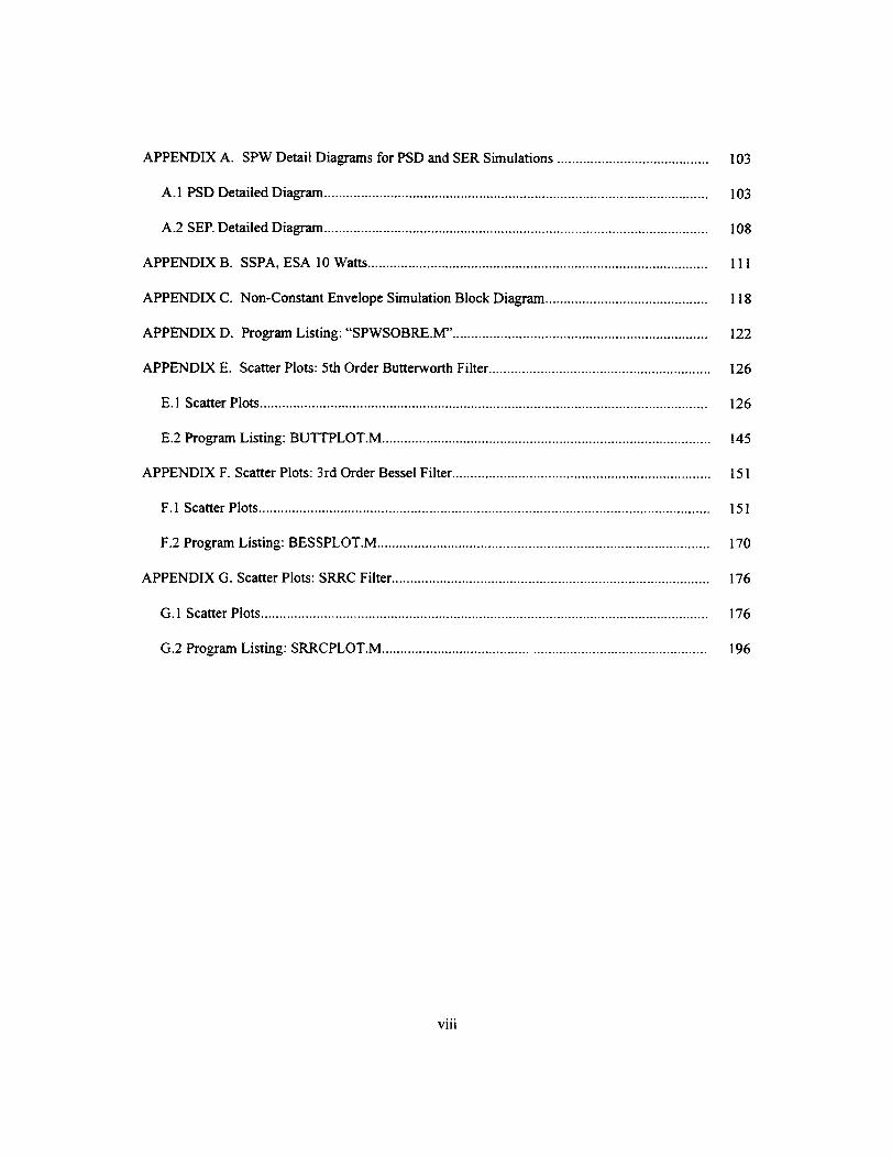
APPENDIXA. SPWDetailDiagramsforPSDandSERSimulations.........................................103
A.1PSDDetailedDiagram........................................................................................................103
A.2SEP.DetailedDiagram........................................................................................................108
APPENDIXB. SSPA,ESA10Watts............................................................................................111
APPENDIXC. Non-Constant Envelope Simulation Block Diagram ............................................ I 18
APPENDIX D. Program Listing: "SPWSOBRE.M". .................................................................... 122
APPENDIX E. Scatter Plots: 5th Order Butterworth Filter ............................................................ 126
E. i Scatter Plots ......................................................................................................................... 126
E.2 Program Listing: BUTTPLOT.M ......................................................................................... 145
APPENDIX F. Scatter Plots: 3rd Order Bessel Filter ...................................................................... 151
F. 1 Scatter Plots .......................................................................................................................... 151
F.2 Program Listing: BESSPLOT.M .......................................................................................... 170
APPENDIX G. Scatter Plots: SRRC Filter ...................................................................................... 176
G. 1 Scatter Plots ......................................................................................................................... 176
G.2 Program Listing: SRRCPLOT.M ........................................................................................ 196
viii
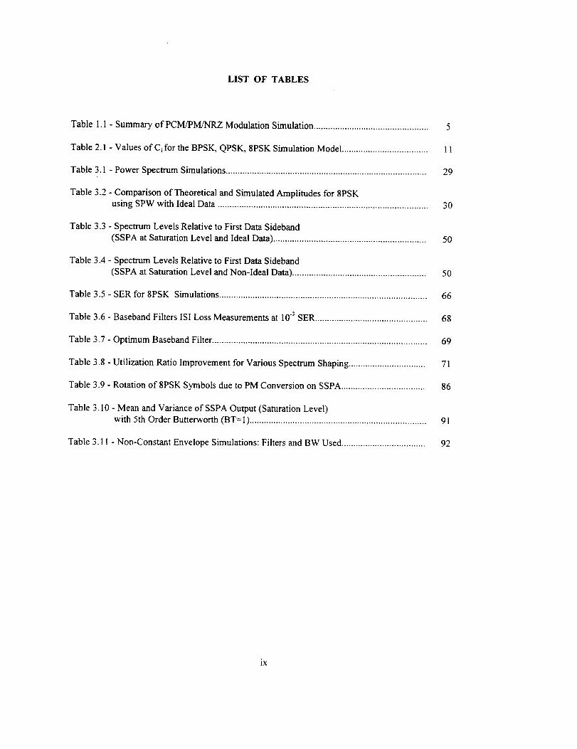
LISTOF TABLES
Table1.1- SummaryofPCM/PM/NRZModulationSimulation................................................5
Table2.1- ValuesofCifortheBPSK,QPSK,8PSKSimulationModel....................................11
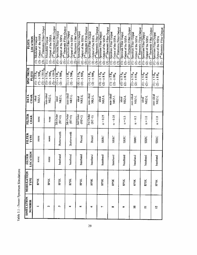
Table 3.1 - Power Spectrum Simulations .................................................................................... 29
Table 3.2 - Comparison of Theoretical and Simulated Amplitudes for 8PSKusing SPW with Ideal Data ........................................................................................ 30
Table 3.3 - Spectrum Levels Relative to First Data Sideband
(SSPA at Saturation Level and Ideal Data) ................................................................ 50
Table 3.4 - Spectrum Levels Relative to First Data Sideband
(SSPA at Saturation Level and Non-Ideal Data) ........................................................ 50
Table 3.5 - SER for 8PSK Simulations ....................................................................................... 66
Table 3.6 - Baseband Filters ISI Loss Measurements at 10 -3 SER ............................................... 68
Table 3.7 - Optimum Baseband Filter .......................................................................................... 69
Table 3.8 - Utilization Ratio Improvement for Various Spectrum Shaping ................................ 71
Table 3.9 - Rotation of 8PSK Symbols due to PM Conversion on SSPA ................................... 86
Table 3.10 - Mean and Variance of SSPA Output (Saturation Level)with 5th Order Butterworth (BT=I) .......................................................................... 91
Table 3.11 - Non-Constant Envelope Simulations: Filters and BW Used ................................... 92
ix
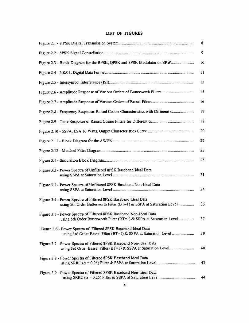
LIST OF FIGURES
Figure 2. I - 8 PSK Digital Transmission System ........................................................................ 8
Figure 2.2 - 8PSK Signal Constellation ....................................................................................... 9
Figure 2.3 - Block Diagram for the BPSK, QPSK and 8PSK Modulator on SPW ...................... 10
Figure 2.4 - NRZ-L Digital Data Format ..................................................................................... 11
Figure 2.5 - Intersymbol Interference (ISI) ................................................................................. 13
Figure 2.6 - Amplitude Response of Various Orders of Butterworth Filters ............................... 15
Figure 2.7 - Amplitude Response of Various Orders of Bessel Filters ........................................ 16
Figure 2.8 - Frequency Response: Raised Cosine Characteristics with Different a .................... 17
Figure 2.9 - Time Response of Raised Cosine Filters for Different ct ......................................... 18
Figure 2.10 - SSPA, ESA 10 Watts, Output Characteristics Curve ............................................. 20
Figure 2.1 ! - Block Dia_am for the AWGN .............................................................................. 22
Figure 2.12 - Matched Filter Diagram ......................................................................................... 23
Figure 3.1 - Simulation Block Diagram ....................................................................................... 25
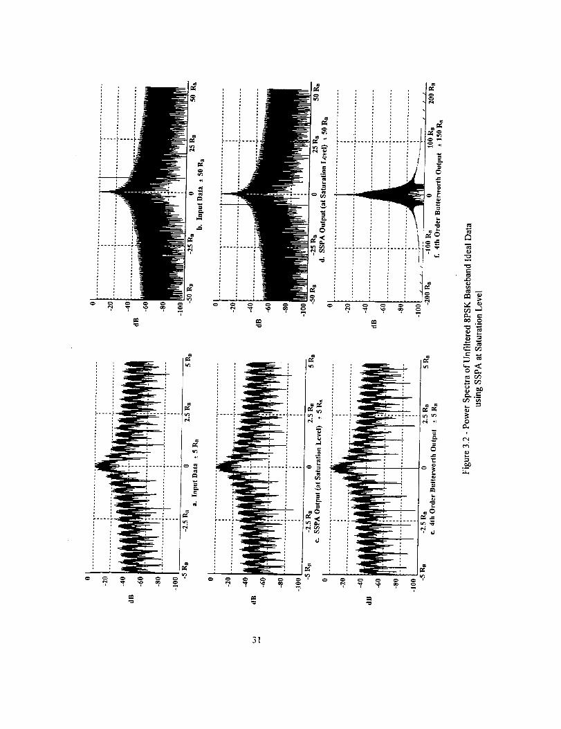
Figure 3.2 - Power Spectra of Unfiltered 8PSK Baseband Ideal Data
using SSPA at Saturation Level .............................................................................. 31
Figure 3.3 - Power Spectra of Unfiltered 8PSK Baseband Non-Ideal Data
using SSPA at Saturation Level .............................................................................. 34
Figure 3.4 - Power Spectra of Filtered 8PSK Baseband Ideal Data
using 5th Order Butterworth Filter (BT=I) & SSPA at Saturation Level ............... 36
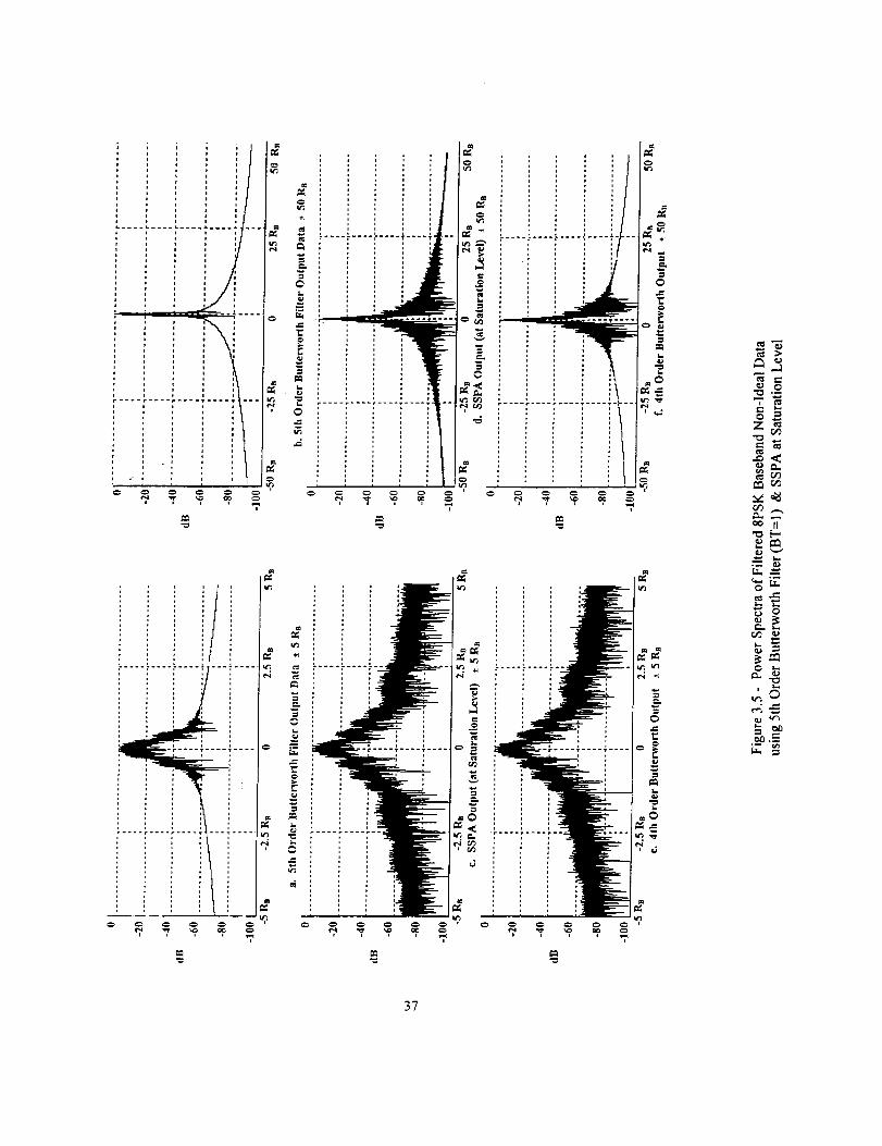
Figure 3.5 - Power Spectra of Filtered 8PSK Baseband Non-Ideal Data
using 5th Order Butterworth Filter (BT=I) & SSPA at Saturation Level .............. 37
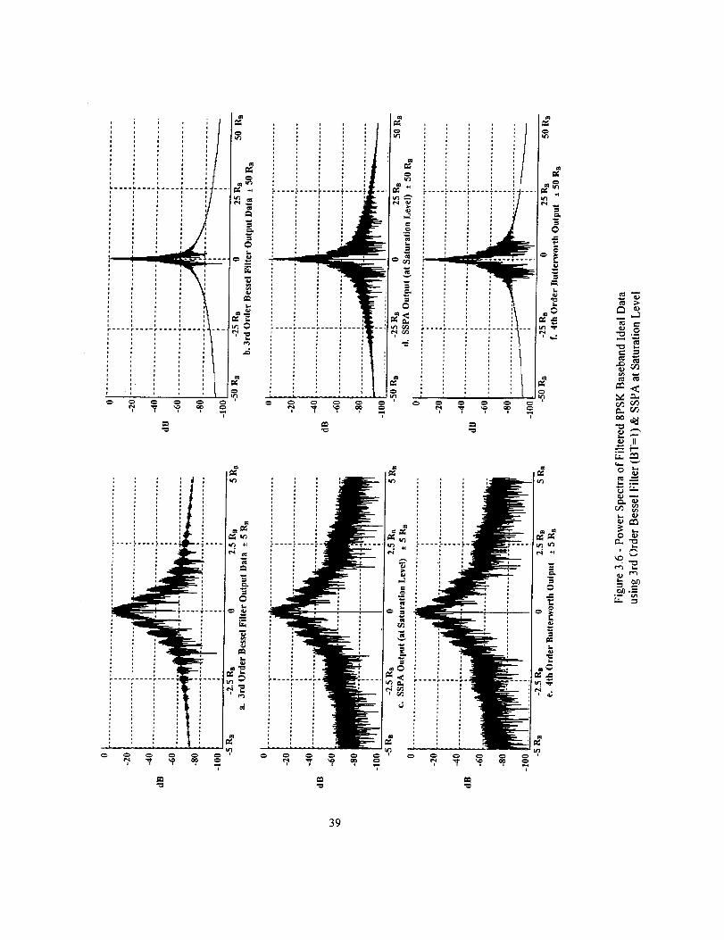
Figure 3.6 - Power Spectra of Filtered 8PSK Baseband Ideal Data
using 3rd Order Bessel Filter (BT=I) & SSPA at Saturation Level ..................... 39
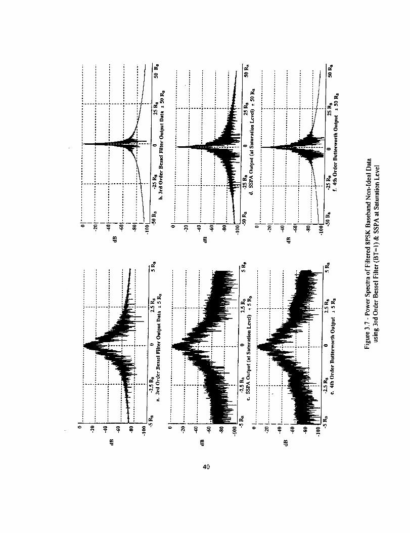
Figure 3.7 - Power Spectra of Filtered 8PSK Baseband Non-ldeal Data
using 3rd Order Bessel Filter (BT=I) & SSPA at Saturation Level ....................... 40
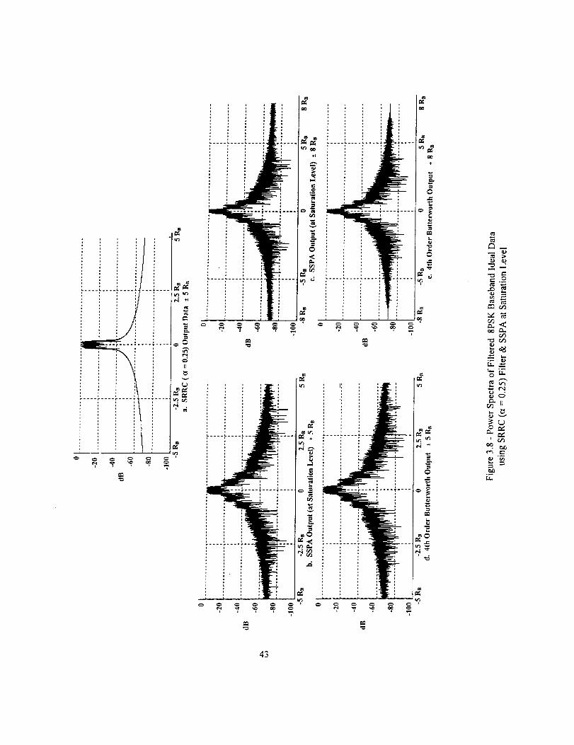
Figure 3.8 - Power Spectra of Filtered 8PSK Baseband Ideal Datausing SRRC (ct = 0.25) Filter & SSPA at Saturation Level .................................... 43
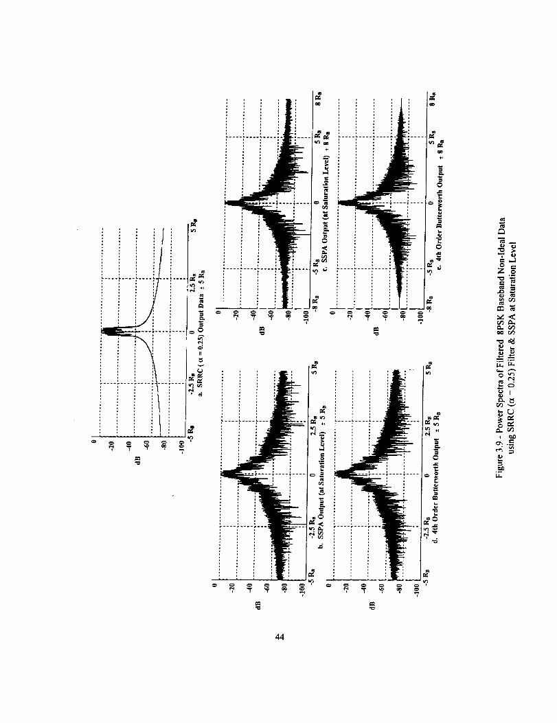
Figure 3.9 - Power Spectra of Filtered 8PSK Baseband Non-Ideal Data
using SRRC (a = 0.25) Filter & SSPA at Saturation Level .................................. 44
X
Figure 3.10 - Power Spectra of Filtered 8PSK Baseband Ideal Data
using SRRC (a = 0.5) Filter & SSPA at Saturation Level ....................................
Figure 3.11 - Power Spectra of Filtered 8PSK Baseband Non-Ideal Data
using SRRC (et = 0.5) Filter & SSPA at Saturation Level ....................................
Figure 3.12 - Power Spectra of Filtered 8PSK Baseband Ideal Data
using SRRC (a = 1) Filter & SSPA at Saturation Level ......................................
Figure 3.13 - Power Spectra of Filtered 8PSK Baseband Non-Ideal Data
using SRRC (ct = I) Filter & SSPA at Saturation Level ........................................
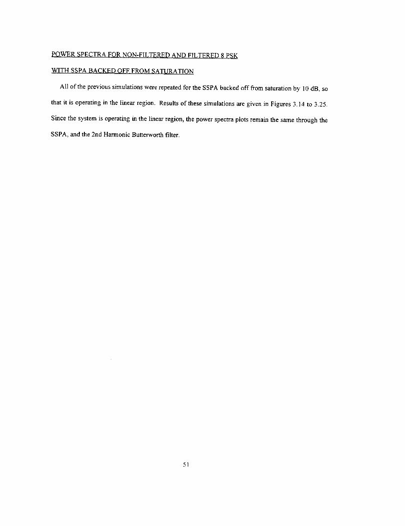
Figure 3.14 - Power Spectra of Unfiltered 8PSK Baseband Ideal Data
using SSPA at 10dB backoff ...............................................................................
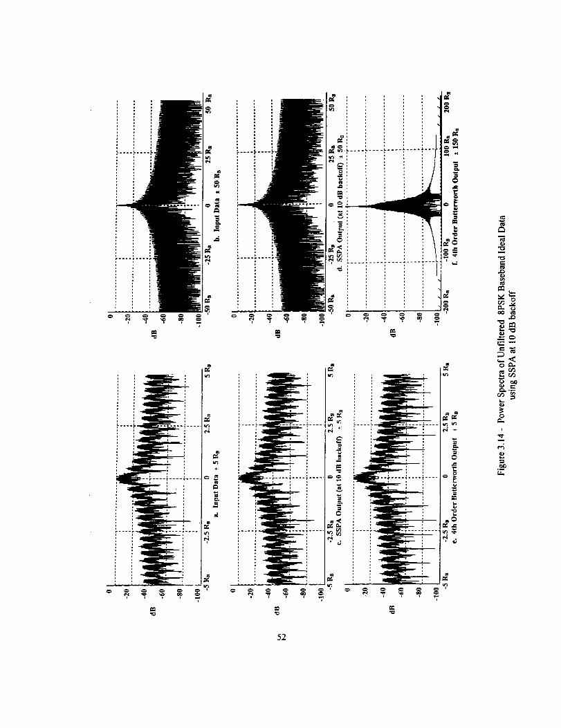
Figure 3.15 - Power Spectra of Unfiltered 8PSK Baseband Non-Ideal Data
using SSPA at 10dB backoff ................................................................................
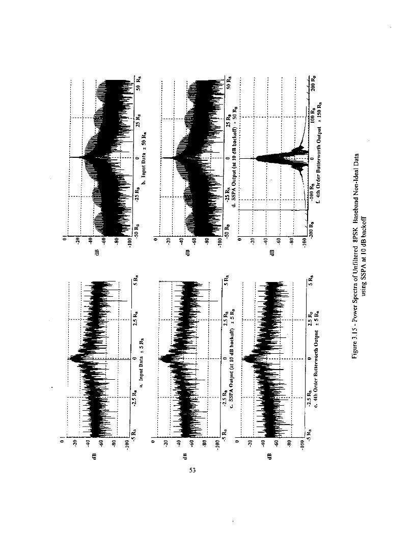
Figure 3.16 - Power Spectra of Filtered 8PSK Baseband Ideal Data
using 5th Order Butterworth Filter (BT=I) & SSPA at 10dB backoff .................
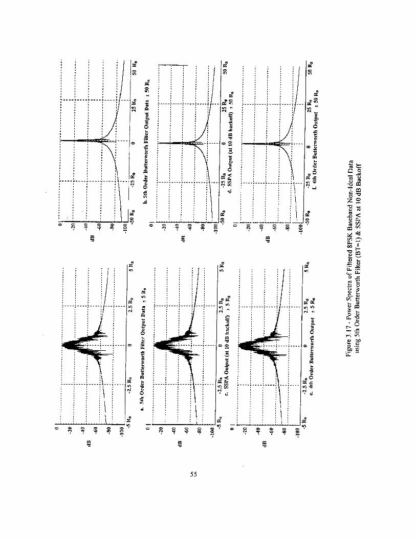
Figure 3.17 - Power Spectra of Filtered 8PSK Baseband Non-Ideal Data
using 5th Order Butterworth Filter (BT=I) & SSPA at 10dB backoff ..................
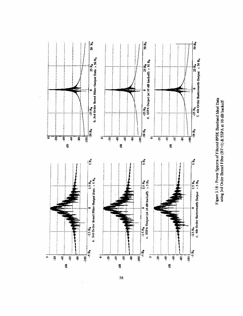
Figure 3.18 - Power Spectra of Filtered 8PSK Baseband Ideal Data
using 3rd Order Bessel Filter (BT=I) & SSPA at 10dB backoff ...........................
Figure 3.19 - Power Spectra of Filtered 8PSK Baseband Non-Ideal
using 3rd Order Bessel Filter (BT=I) & SSPA at 10dB backoff .........................
Figure 3.20 - Power Spectra of Filtered 8PSK Baseband Ideal Data
usmg SRRC Filter (a = 0.25) & SSPA at 10dB backoff. ......................................
Figure 3.21 - Power Spectra of Filtered 8PSK Baseband Non-Ideal Data
using SRRC (ct = 0.25) Filter & SSPA at 10dB backoff ......................................
Figure 3.22 - Power Spectra of Filtered 8PSK Baseband Ideal Data
using SRRC (c_ = 0.5) Filter & SSPA Filter at 10dB backoff ...............................
Figure 3.23 - Power Spectra of Filtered 8PSK Baseband Non-Ideal Data:
using SRRC (a = 0.5) Filter & SSPA at 10dB backoff .......................................
Figure 3.24 - Power Spectra of Filtered 8PSK Baseband Ideal Data
using SRRC (a = I) Filter & SSPA at 10dB backoff ...........................................
Figure 3.25 - Power Spectra of Filtered 8PSK Baseband Non-Ideal Data
using SRRC (ct = 1) Filter & SSPA at 10dB backoff ...........................................
Figure 3.26 - SER for 8PSK curves: Ideal and Non-Ideal Data with BT = oo.............................
46
47
48
49
52
53
54
55
56
57
58
59
60
61
62
63
65
xi
Figure3.27- SER for 8PSK: 5th Order Butterworth BT = 1, 2 and 3
(SSPA at Saturation & Ideal Data) ......................................................................... 67
Figure 3.28 - SER for 8PSK: 3rd Order Bessel BT = 1, 2 and 3
(SSPA at Saturation & Ideal Data) ......................................................................... 67
Figure 3.29 - SER for 8PSK: SRRC ct = 1 (no SSPA), a = 0.25, 0.5, and 1(SSPA at Saturation & Ideal Data) ........................................................................ 68
Figure 3.30 - 8PSK Modulator Output: Real & Imaginary Part ............................................... 75
Figure 3.31 - 8PSK Modulator Output: Magnitude & Phase ...................................................... 76
Figure 3.32 - 5th Order Butterworth Filter (BT = 1) Output: Real & Imaginary Part ................ 77
Figure 3.33 - 5th Order Butterworth Filter (BT = 1) Output: Magnitude & Phase ..................... 78
Figure 3.34 - Output of SSPA (Input = Output of 5th Order Butterworth Filter (BT = I))
Real & Imaginary Part .......................................................................................... 79
Figure 3.35 - Output of SSPA (Input = Output of 5th Order Butterworth Filter (BT = 1))
Magnitude & Phase ............................................................................................... 80
Figure 3.36 - Output of SSPA (Input = Output of 8PSK Modulator (Constant Envelope))
Real & Imaginary Part .......................................................................................... 81
Figure 3.37 - Output of SSPA (Input = Output of 8PSK Modulator (Constant Envelope))
Magnitude & Phase ............................................................................................... 82
Figure 3.38 - Non-Constant Envelope Simulations Block Dia_am ........................................... 84
Figure 3.39 - SSPA, ESA 10 Watts, Zoomed Magnitude Characteristic Curve ......................... 84
Figure 3.40 - SSPA, ESA 10 Watts, Phase (degrees) Characteristic Curve ................................ 85
Figure 3.41 - Scatter Plot: 8PSK Modulator, 5th Order Butterworth Filter (BT = 1), and SSPA
(Saturation Level) Output ...................................................................................... 87
Figure 3.42 - Mean and Variance in Decision Region ................................................................. 91
Figure 3.43 - 5th Order Butterworth Filter: Average Symbol Variance vs. BT .......................... 93
Figure 3.44 - Zoom of Average Symbol Variance vs. BT for 5th Order Butterworth Filter ....... 94
Figure 3.45 - 3rd Order Bessel Filter: Average Symbol Variance vs. BT ................................... 95
Figure 3.46 - Zoom of Average Symbol Variance vs. BT for 3rd Order Bessel Filter ................ 95
Figure 3.47 - SRRC Filter: Average Symbol Variance vs. Rolloff Factor (a) ............................ 96
xii
LIST OF ABBREVIATIONS
a orr
9
AM
AWGN
ASCII
dB
BER
Bi-_b
BPSK
BW
BT
CCSDS
DC
Es/No
ESA
fs
FFT
FSK
FSE
FTP
GMSK
Hz
HP
Rolloff Factor for SRRC filters
Band Utilization Ratio
Amplitude Modulation
Additive White Gaussian Noise
American Information Code for Information Interchange
Decibels
Bit Error Rate
Bi-Phase (Manchester)
Binary Phase Shift Keying
Bandwidth
Bandwidth-Time (symbol) product
Consultative Committee for Space Data Systems
Direct Current
Energy (symbol) to Noise ratio
European Space Agency
Sampling Frequency
Fast Fourier Transform
Frequency Shift Keying
Fractionally-Spaced Equalizer
File Transfer Protocol
Gaussian Minimum Shift Keying
Hertz
Hewlett Packard
xiii
IF
IIR
ISl
JPL
LSB
MSB
MSK
NASA
NMSU
NRZ-L
OQPSK
PA
PC
PCM
PM
PSD
PSK
QPSK
RB
Rs
RC
RF
sec
SER
SFCG
Intermediate Frequency
Infinite Impulse Response (filter)
InterSymbol Interference
Jet Propulsion Laboratory
Least Significant Bit
Most Significant Bit
Minimum Shift Keying
National Aeronautics and Space Administration
New Mexico State University
Non-Return-to-Zero Logic
Offset Quaternary Phase Shift Keying
Power Amplifier
Personal Computer
Pulse Coded Modulation
Phase Modulation
Power Spectral Density
Phase Shift Keying
Quartenary Phase Shift Keying
Bit Rate
Symbol or Baud Rate
Raised Cosine
Radio Frequency
Seconds
Symbol Error Rate
Space Frequency Coordination Group
xiv
SNR
SPC
SPW
SSPA
SRRC
TB
TWT
V
Signal-to-NoiseRatio
Serial-to-ParallelConverter
SignalProcessingWorksystem
SolidStatePowerAmplifier
SquareRootRaisedCosine
BitPeriod
TravelingWaveTube
Volts
XV
Chapter 1
INTRODUCTION AND BACKGROUND
This thesis gives the results of a study on 8 Level Phase Shift Keying (8PSK) modulation with
respect to bandwidth, power efficiency, spurious emissions, interference susceptibility and the non-
constant envelope effect through a non-linear channel. This work was conducted at New Mexico State
University (NMSU) in the Center for Space Telemetering and Telecommunications Systems in the
Klipsch School of Electrical and Computer Engineering Department and is supported by a grant from
the National Aeronautics and Space Administration (NASA) # NAG 5-1491.
The first chapter of this report gives a brief summary of the work completed by the Jet Propulsion
Laboratory (JPL) on various modulation schemes and previous studies performed on non-constant
envelope signals. In Chapter 2, some theoretical concepts will be explained which are directly related
to the simulations that were performed for the gPSK modulation. Finally in Chapter 3, results on the
simulations for 8PSK will be given. The simulations were performed on a Signal Processing
Worksystem (SPW) * (software installed on a SUN SPARC l0 Unix Station and Hewlett Packard
Model 715/100 Unix Station) where the power containment, spurious emissions, symbol error rates
and non-constant envelope effect on the bandwidth are measured for different types of spectrum
shaping filters. Conclusions and suggestions for further work are given at the end of this report in
Chapter 4.
* SPW is a registered trademark of COMDISCO systems, a Business Unit of Cadence Design Systems,
Inc. 919 East Hillsdale Blvd., Foster City, CA 94404.
Duringits12thannualmeeting(November1992inAustralia),theSpaceFrequencyCoordination
Group(SFCG-12)requestedtheConsultativeCommitteefor SpaceDataSystems(CCSDS)Radio
Frequency(RF)andModulationSubpanelto studyandcomparevariousmodulationschemeswith
respectto: (a)- bandwidth needed;
(b) - power efficiency;
(c) - spurious emissions; and
(d) - interference susceptibility.
This study has to be conducted due to the fact that frequency bands are becoming more and more
congested and space agencies are under constant pressure to reduce costs. To date, four position
papers have been presented (References [I], [2], [3], and [4]). These reports divided the study into
three logical phases:
Phase I (a) - Bandwidth (BW) utilization of various modulation schemes, explores traditional
modulation schemes that were used in the past and compares them with newer ones that could improve
the communication channel efficiencies. From this fu'st paper, the following was concluded. The
traditional modulation methods utilize subcarriers which have some advantages and disadvantages.
The subcarrier greatly facilitates the separation of data types and also separates the data transmitted
from the RF carrier. On the other hand, subcarriers significantly increased the spacecraft complexity.
It also produces additional losses in the modulator and demodulator and occupies a large bandwidth.
The new modulation techniques (and data formatting) such as PCM/PM/Bi-_ (Pulse Coded
Modulated/Phase Modulation: data are Bi-Phase (Manchester) modulated directly on a residual RF
carrier), PCM/PM/NRZ (NRZ data are phase modulated directly on a residual RF carrier), BPSK/Bi-qb
(data is Bi-Phase (Manchester) modulated on an RF carrier full), suppressing it) and BPSK/NRZ
(Binary Phase Shift Keying/NRZ data is phase modulated directly on an RF carrier fully suppressing
it) were examined.
It wasnoted,asexpected, that these new types of modulation significantly reduce the amount of
BW. Therefore use of subcarriers should be limited. A new definition of required bandwidth was
proposed (required BW is equal to 95% of the corresponding ideally modulated square pulse shaping
signal) due to the ambiguities of the present definitions. For more information refer to [ 1].
Phase I (b) - A comparison of Quartenary Phase Shift Keying (QPSK), Offset Quartenary Phase
Shift Keying (OQPSK), BPSK, and Gaussian Minimum Shift Keying (GMSK) [2] is a complimentary
paper for Phase I (a) which studies modulations that seem more promising for this study (BPSK was
used as reference). First, it was concluded that by doing some spectral shaping on the data, a
reduction of the bandwidth can be achieved. The unfiltered data spec_um can be as much as 5 to 10
times the width of the filtered data specu'um. Also the signal degradation due to power losses, pulse
distortions and ISI is between 0.2 and 0.4 dB (for QPSK, OQPSK, BPSK, and GMSK) if a matched
receiver is used. With respect to the pulse shaping filtering, it was mentioned that such filtering at the
Intermediate Frequency (IF) level would require hardware that would be considered acceptable for RF
filtering. With respect to the modulation schemes it was noticed that GMSK is a bit better than QPSK
and filtered BPSK in non-linear channels unless filtering is applied after the power amplifier (PA). In
the case of pulse shaping filtering, the GMSK and filtered OQPSK offered practically identical
performance.
Phase II - Spectrum Shaping [3] is analyzed and simulated. The benefits accruing from the
spectrum shaping of the transmitted signal are presented. This paper shows that several types of filters
and location for these filters can be used. Also it was shown that spectrum shaping, with an efficient
type of modulation, can increase the utilization ratio. This would allow more signals to be placed into
a given frequency band. The paper also gives the frequency spectra simulations performed on
PCM/PM/NRZ data on the SPW (COMDISCO) simulation software. Non-ideal and ideal data were
used with 4 different types of spectrum shaping filters (Butterworth 5th Order, Bessel 3rd Order,
Raised Cosine (ct = 0.25, 0.5 and l with NRZ-L data and sampled data), SRRC (co = 1 with NRZ-L
dataandsampleddata)).All thesesimulationswereperformedusinga non-idealsystemandat
passband.PowerSpectralplots(PowerContainmentversusRB) weregeneratedforthesedifferent
typesoffiltersattheoutputofthebasebandfilter,SSPAand2ndHarmonicfilter(referto [3] for more
information) and were compared with the case where no baseband filtering is performed. It was
shown that this baseband filtering in fact improves the frequency band Utilization Ratio. Studies were
also performed to determine the filter amplitude response and ISI of these filters. The Raised Cosine
filter was found to be amplitude unstable at high data transition rates therefore it was not included in
Phase III.
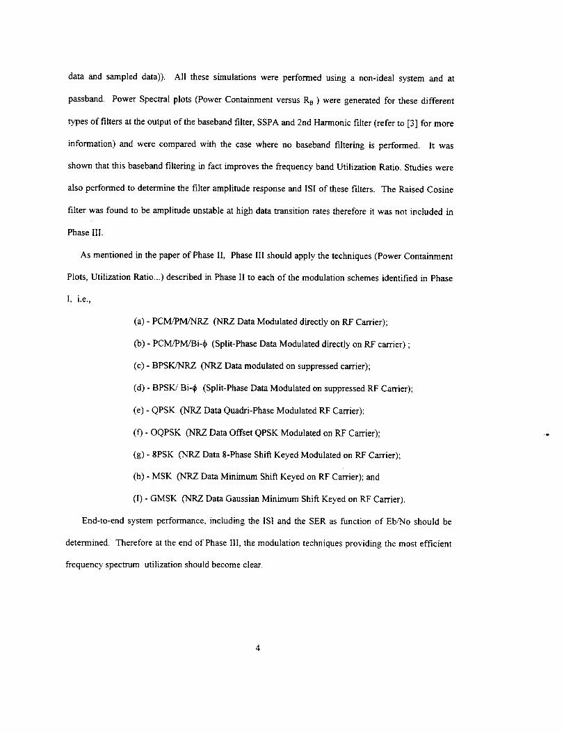
As mentioned in the paper of Phase I1, Phase IIl should apply the techniques (Power Containment
Plots, Utilization Ratio...) described in Phase II to each of the modulation schemes identified in Phase
I, i.e.,
(a) - PCM/PM/NRZ (NRZ Data Modulated directly on RF Carrier);
(b) - PCM/PM/Bi-_b (Split-Phase Data Modulated directly on RF carrier) ;
(c) - BPSK/NRZ (NRZ Data modulated on suppressed carrier);
(d) - BPSK/Bi-dp (Split-Phase Data Modulated on suppressed RF Carrier);
(e) - QPSK (NR.Z Data Quadri-Phase Modulated RF Carrier);
(f) - OQPSK (NRZ Data Offset QPSK Modulated on RF Carrier);
(g) - 8PSK (NRZ Data 8-Phase Shift Keyed Modulated on RF Carrier);
(h) - MSK (NRZ Data Minimum Shift Keyed on RF Carrier); and
(I) - GMSK (NRZ Data Gaussian Minimum Shift Keyed on RF Carrier).
End-to-end system performance, including the ISI and the SER as function of Eb/No should be
determined. Therefore at the end of Phase III, the modulation techniques providing the most efficient
frequency spectrum utilization should become clear.
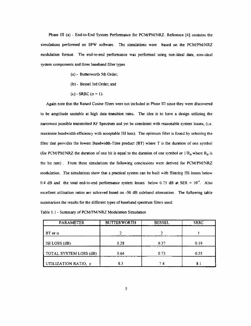
PhaseIII (a)- End-to-End System Performance for PCM/PM/NRZ. Reference [4] contains the
simulations performed on SPW software. The simulations were based on the PCM/PM/NRZ
modulation format. The end-to-end performance was performed using non-ideal data, non-ideal
system components and three baseband filter types
(a) - Buttervcorth 5th Order;
(b) - Bessei 3rd Order; and
(c) - SRRC (_ = 1).
Again note that the Raised Cosine filters were not included in Phase III since they were discovered
to be amplitude unstable at high data transition rates. The idea is to have a design utilizing the
narrowest possible transmitted RF Spectrum and yet be consistent with reasonable system losses, (i.e.
maximize bandwidth efficiency with acceptable ISI loss). The optimum filter is found by selecting the
filter that provides the lowest Bandwidth-Time product (BT) where T is the duration of one symbol
(for PCM/PM/NRZ the duration of one bit is equal to the duration of one symbol or 1/R Bwhere RB is
the bit rate) . From these simulations the following conclusions were derived for PCM/PM/NRZ
modulation. The simulations show that a practical system can be built with filtering ISl losses below
0.4 dB and the total end-to-end performance system losses below 0.75 dB at SER = 10"3. Also
excellent utilization ratios are achieved based on -50 dB sideband attenuation. The following table
summarizes the results for the different types of baseband spectrum filters used:
Table 1.1 - Summary of PCM/PM/NRZ Modulation Simulation
PARAMETER BUTTERWORTH BESSEL SRRC
BT or a 2 2 1
ISI LOSS (dB) 0.28 0.37 0.19
TOTAL SYSTEM LOSS (dB) 0.64 0.73 0.55
UTILIZATION RATIO, p 8.5 7.4 8.1
Asshowninthistable,significantbandwidthsavings(UtilizationRatio)ispossiblebyselecting
theproperbasebandfilter.Differentmodulationtypeswill alsoaffectthebandwidthsavings.
Therefore,futureworkwill involvethesamemeasurementsasdescribedaboveforthedifferenttypes
ofmodulation.Itwill thenbepossibletoidentifythemostefficientmodulationtype(s)baseduponthe
application,thesystemperformanceandthepreferredfrequencyband. In thiscase, thisreport
containsthesimulationsperformedonan8PSKsignalbeingfiltered(spectrumshaping)bythethree
filtersmentionedearlier.
Tocompletethiswork, therelationshipbetweenthenon-constantenvelopeintroducedbypulse
shapingthe8PSKsignalandthebandwidthof thefilter wasto be investigated.Thereforethe
followingquestionhadtobeanswered:
How much variation is introduced by the non-constant envelope
as the bandwidth of the filter is made smaller?
A literature search was conducted to see if any kind of investigation had been performed with
respect to an 8PSK non-constant envelope signal going through a non-linear channel (amplifier). The
analysis of the non-linear distortion caused by the amplifier, more specifically for a non-constant
envelope, is very complicated. Although many analyses have been published in the literature, none
has been entirely applicable here. The research conducted in [5] shows how a bandlirnited spectrum
filter and the shape of the frequency pulse affect the error probability of a frequency shift keying
(FSK) signal with differential phase detection. The investigation was conducted using a Butterworth
filter (order = 4 and 3 for the transmitter and receiver respectively) and the frequency shaping pulse is
raised cosine or rectangular. This investigation was then performed for a FSK signal as opposed to a
PSK signal. In [6], an experiment more related to the one described in this thesis was performed.
This paper investigates the effect of filtering PSK, FSK and MSK signals in a theoretical way. A
Butterworth Filter (4th Order) is used and the ISI and BER are measured.
6
However, this paper does not consider an amplifier in their study. In [7], the performance of a
satellite channel using a software package (developed at Telecom Research Laboratories) was
measured.
The results of this experiment (using the software) were then validated by experiments on a
hardware simulator. It was shown that both results from the software and actual measurements are
very similar (minor differences due to the ideal demodulator used in the software package). Even
though the satellite channel in this paper uses spectrum shaping filters and non-linearities (TWT
Amplifier), there was no experiment conducted to measure the effect of non-constant envelope
through this non-linear system.
Although other similar studies were performed on pulse shaping, non-constant envelope and non-
linear channels, none of them involved the measurement of the effect of a non-constant envelope
signal (8PSK for this case) through a non-linear channel (SSPA). The following thesis gives the
results on simulations performed on an 8PSK bandlimited signal ( bandlimited with the three filters
enumerated earlier) going through a non-linear amplifier. The effect of the non=constant envelope
through this channel will be demonstrated.
Chapter 2
THEORY
This section will briefly describe some of the concepts that were used for the simulations performed
on the SPW simulation software (from COMDISCO) that is installed on a SUN Sparc Station l0 and
HP Model 715/100 Unix Station in the Center for Space Telemetering and Telecommunications
Systems in the Klipsch School of Electrical and Computer Engineering Department at NMSU.
2. 1 Eight (8) Level Phase Shift Keying (8PSK)
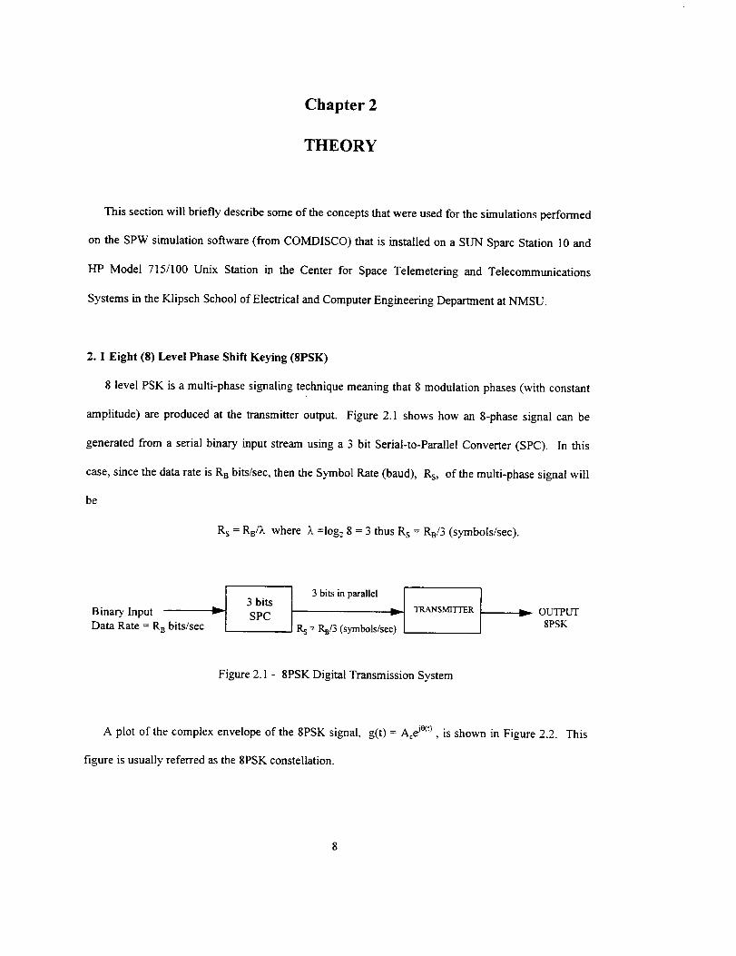
8 level PSK is a multi-phase signaling technique meaning that 8 modulation phases (with constant
amplitude) are produced at the transmitter output. Figure 2.1 shows how an 8-phase signal can be
generated from a serial binary input stream using a 3 bit Serial-to-Parallel Converter (SPC). In this
case, since the data rate is RB bits/sec, then the Symbol Rate (baud), Rs, of the multi-phase signal will
be
Rs = RB/X where X =log2 8 = 3 thus Rs = RB/3 (symbols/sec).
3 bitsBinary Input _- SPC
Data Rate = Ra bits/sec
3 bits in parallel v_
Rs ---I_/3 (symbols/see)
TRANSMITTER
Figure 2. I - 8PSK Digital Transmission System
I -.-- OUTPUT8PSK
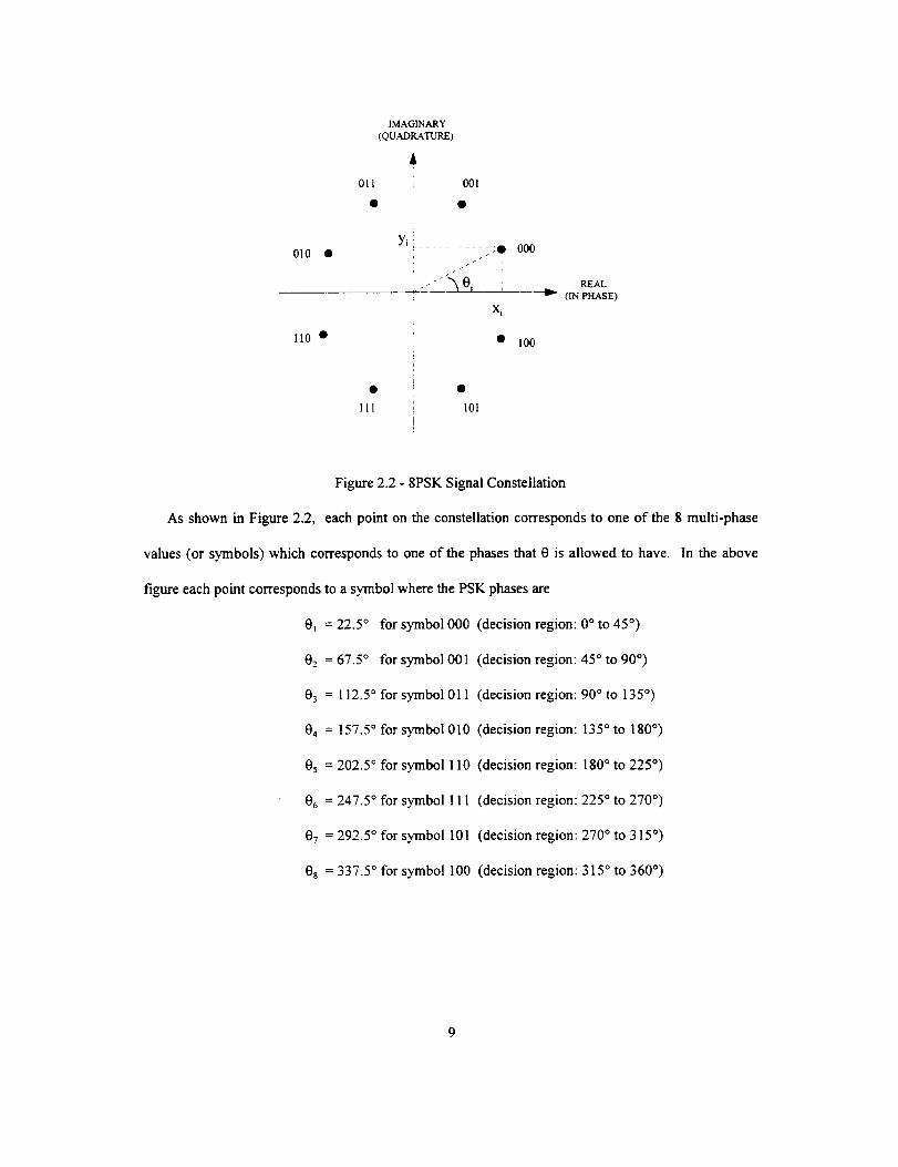
A plot of the complex envelope of the 8PSK signal, g(t) = Ace _°<_), is shown in Figure 2.2. This
figure is usually referred as the 8PSK constellation.
IMAGINARY
(QUADRATURE)
A
011 001
OlO •
i10 •
lll
Yiooo
X i
• 100
101
REAL
_- (IN PHASE)
Figure 2.2 - 8PSK Signal Constellation
As shown in Figure 2.2, each point on the constellation corresponds to one of the 8 multi-phase
values (or symbols) which corresponds to one of the phases that 0 is allowed to have. In the above
figure each point corresponds to a symbol where the PSK phases are
0t = 22.5 ° for symbol 000
02 = 67.5 ° for symbol OOl
03 = 112.5 ° for symbol 0l 1
(decision region: 0° to 45 °)
(decision region: 45 ° to 90 °)
(decision region: 90 ° to 135 °)
04 = 157.5 ° for symbol 010 (decision region: 135 ° to 180 °)
05 = 202.5 ° for symbol 110 (decision region: 180 ° to 225 °)
06 = 247.5 ° for symbol 111 (decision region: 225 ° to 270 °)
07 = 292.5 ° for symbol 101 (decision region: 270 ° to 315 °)
Os = 337.5 ° for symbol 100 (decision region: 315 ° to 360 °)
9
Anotherway of expressing 8PSK is by using two orthogonal carriers modulated by x and y
components of the complex envelope (no phase modulator is used in this case) thus
g(t) = Ace/°(t) = x(t) + jy(t)
where x i = A c cos 0i and y_ = A c sin 0i where i = 1 to 8 for 8PSK as shown in Figure 2.2.
For the bandpass physical signal, the waveform can then be represented by
v(t) = Re{g(t)e i°'ct} where c0c= 2rife, fc is the carrier fi'equency in hertz (Hz).
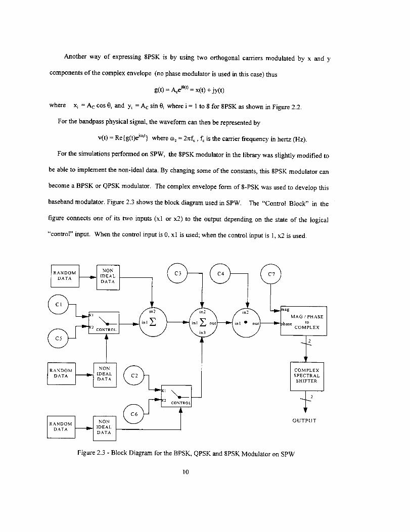
For the simulations performed on SPW, the 8PSK modulator in the library was slightly modified to
be able to implement the non-ideal data. By changing some of the constants, this 8PSK modulator can
become a BPSK or QPSK modulator. The complex envelope form of 8-PSK was used to develop this
baseband modulator. Figure 2.3 shows the block diagram used in SPW. The "Control Block" in the
figure connects one of its two inputs (xl or x2) to the output depending on the state of the logical
"control" input. When the control input is 0, x 1 is used; when the control input is 1, x2 is used.
_Ur_hag MAG ! PHASE
ase COMPLEX
I COMPLEX
SPECTRAL
SHIFTER
OUTPUT
Figure 2.3 - Block Diagram for the BPSK, QPSK and 8PSK Modulator on SPW
10
Thevaluesof Ci are given in Table 2.1 and vary depending on the desired modulator (BPSK,
QPSK or 8-PSK)
Table 2.1 - Values of C_ for the BPSK, QPSK, 8PSK Simulation Model
MODULATION VALUES OF CONSTANT "Ci"
TYPE C 1 "C2 C3 C4 C5 C6 C7
BPSK 0.0 0.0 0.0 2n/2 0.0 0.0 4"2
QPSK 2.0 0.0 0.5 2zc/4 0.0 0.0
8PSK 2.0 4.0 0.5 2_/8 0.0 0.0 _/_
2.2 NRZ-L Ideal And Non-Ideal Data
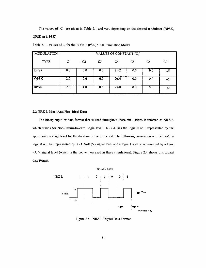
The binary input or data format that is used throughout these simulations is referred as NRZ-L
which stands for Non-Return-to-Zero Logic level. NRZ-L has the logic 0 or 1 represented by the
appropriate voltage level for the duration of the bit period. The following convention will be used: a
logic 0 will be represented by a -A Volt (V) signal level and a logic 1 will be represented by a logic
+A V signal level (which is the convention used in these simulations). Figure 2.4 shows this digital
NRZ-L
data format.
0 Volts
BINARY DATA
i
1 1 , 0i
i
-A
1 0 0 1
Time
i"4"---
Bit Period = T a
Figure 2.4 - NRZ-L Digital Data Format
11
All the simulations were done using ideal and non-ideal data. Ideal data are defined as having a
perfect symmetry, i.e., the duration of a digit one (l) is equal to the time duration of a digit zero (0)
and it also has a perfect data balance, i.e., the probability of getting a zero is equal to the probability of
getting a 1 (Pr(0) = Pr(l) = 0.5 or 50%). For non-ideal data these two conditions, data symmetry and
data balance, are not respected. The CCSDS limits are _+2% for data asymmetry and a data imbalance
of 0.45 (probability of getting a 1 vs probability of a 0) as mentioned in [3]. The data asymmetry can
be increased by the stray capacitance in spacecraft wiring and data imbalance can be produced by long
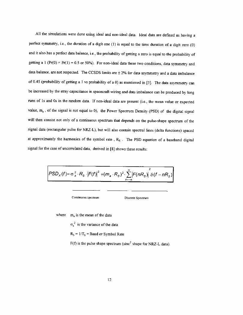
runs of ls and 0s in the random data. If non-ideal data are present (i.e., the mean value or expected
value, ma, of the signal is not equal to 0), the Power Spectrum Density (PSD) of the digital signal
will then consist not only of a continuous spectrum that depends on the pulse-shape spectrum of the
signal data (rectangular pulse for NRZ-L), but will also contain spectral lines (delta functions) spaced
at approximately the harmonics of the symbol rate , Rs . The PSD equation of a baseband digital
signal for the case of uncorrelated data, derived in [8] shows these results:
2 rPSDx(f)=_ 2 .R s .IF(f)I 2 +(m_ .Rs) 2- _ F(nRs) t 5(f -nRs)a fl=-_
Continuous spectrum Discrete Spectrum
where ma is the mean of the data
_a 2 is the variance of the data
Rs = 1/Ts = Baud or Symbol Rate
F(f) is the pulse shape spectrum (sinc e shape for NRZ-L data).
12
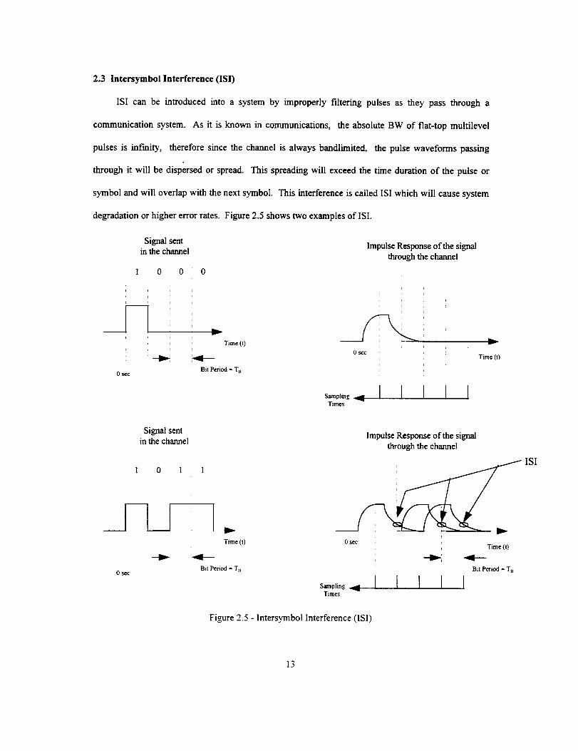
2.3 lntersymbol Interference (ISI)
ISI can be introduced into a system by improperly filtering pulses as they pass through a
communication system. As it is known in communications, the absolute BW of flat-top multilevel
pulses is infinity, therefore since the channel is always bandlimited, the pulse waveforms passing
through it will be dispersed or spread. This spreading will exceed the time duration of the pulse or
symbol and will overlap with the next symbol. This interference is called ISI which will cause system
degradation or higher error rates. Figure 2.5 shows two examples of ISI.
0 sec
Signal sentin the channel
1 0 0 0
v
Time (t)
Bit Period = T R
Impulse Response of the signalthrough the channel
i
i
0 se¢
Sampling _._
Times
I I I I I
v
Time (t)
Signal sentin the channel
0 s_c
1 1
Time (t)
Bit Period = Ya
Sampling
Times
Impulse Response of the signalthrough the channel
i0 s¢¢
Time (1)
Bit Period = T n
I I I I I
ISI
Figure 2.5 - lntersyrnbol Interference (ISI)
13
In 1928,Nyquistdiscoveredthreedifferentmethodsto eliminateIS1byhavingroundedtops
pulsesinsteadoffiattops[8]. TheBWcanthenberestrictedwithoutintroducingISI. Oneofthese
methodsincludestheutilizationofRaisedCosine- RolloffFilteringthatwillbedescribedbelow.
2.4 Spectrum Shaping And Filters
Spectrum Shaping is a technique that allows the signal energy to be concentrated near the carrier
and therefore reduce the power contained in the sidelobes (baseband and RF). This is done by filtering
the signal. Such a technique can also yield a significant savings in the required BW. Nonetheless,
this type of filtering causes loss of energy (if filtering is done at the RF level) and ISI or pulse
distortion (if the BW limitation is too restrictive since the pulses are not rectangular any more). These
losses can be reduced if the receiver compensates for the distortions (i.e., if a matched filter is used).
Thus baseband filtering is effective in limiting spectrum width.
The filters that were used for the simulations are Butterworth, Bessel and Raised Cosine. They will
be described in the following paragraphs.
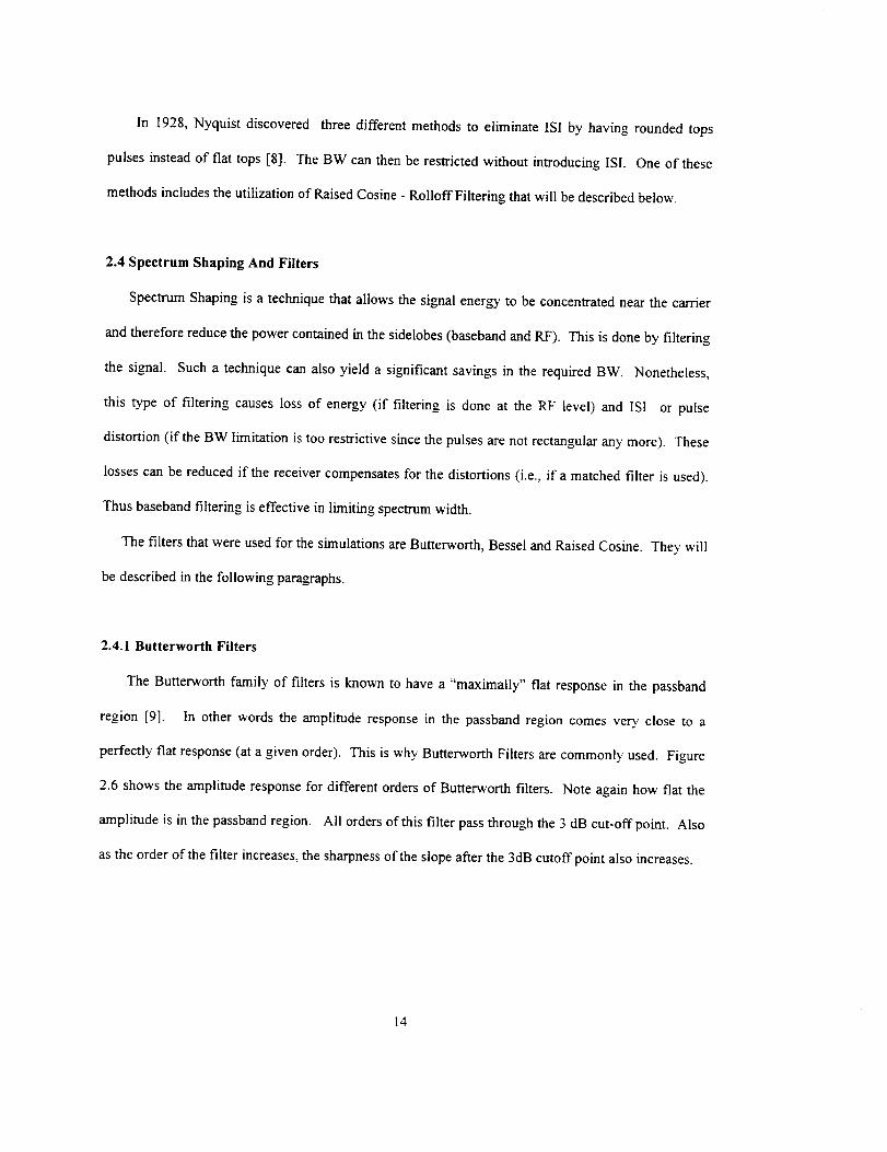
2.4.1 Butterworth Filters
The Butterworth family of filters is known to have a "maximally" flat response in the passband
region [9]. In other words the amplitude response in the passband region comes very. close to a
perfectly flat response (at a given order). This is why Butterworth Filters are commonly used. Figure
2.6 shows the amplitude response for different orders of Butterworth filters. Note again how flat the
amplitude is in the passband region. All orders of this filter pass through the 3 dB cut-offpoint. Also
as the order of the filter increases, the sharpness of the slope after the 3dB cutoff point also increases.
14
BufferworthFilter fc(3dB) = 1 Hz& order=2.3.4.5.6.7.8
o _---_L_, ;,=2 ':
-20 ...................... i...........
-40 ..... ":..... ,----: .... .'-" _..... n=4 : --"_- - - - -'.%;....... "_._---
Cut-Off i / i n = _ :, \ ,,\ :\ -..!60 -Frequency .... iI.i ........................ i____.__.__. _i..._ .....
fc=lHz !l ! n=6 "----Y\,?'\ :', "_ !
.... : \ \ \ :,,
-8o_-.... ].....i---] ...._.................... i ..... ._'z"_'!,i"_'_--_',_--]/ : : ! ! n=8 .-4------/ i'_,\_ i\l
i \, '_/100
Frequency (Hz)
Figure 2.6 - Amplitude Response of Various Orders of Butterworth Filters
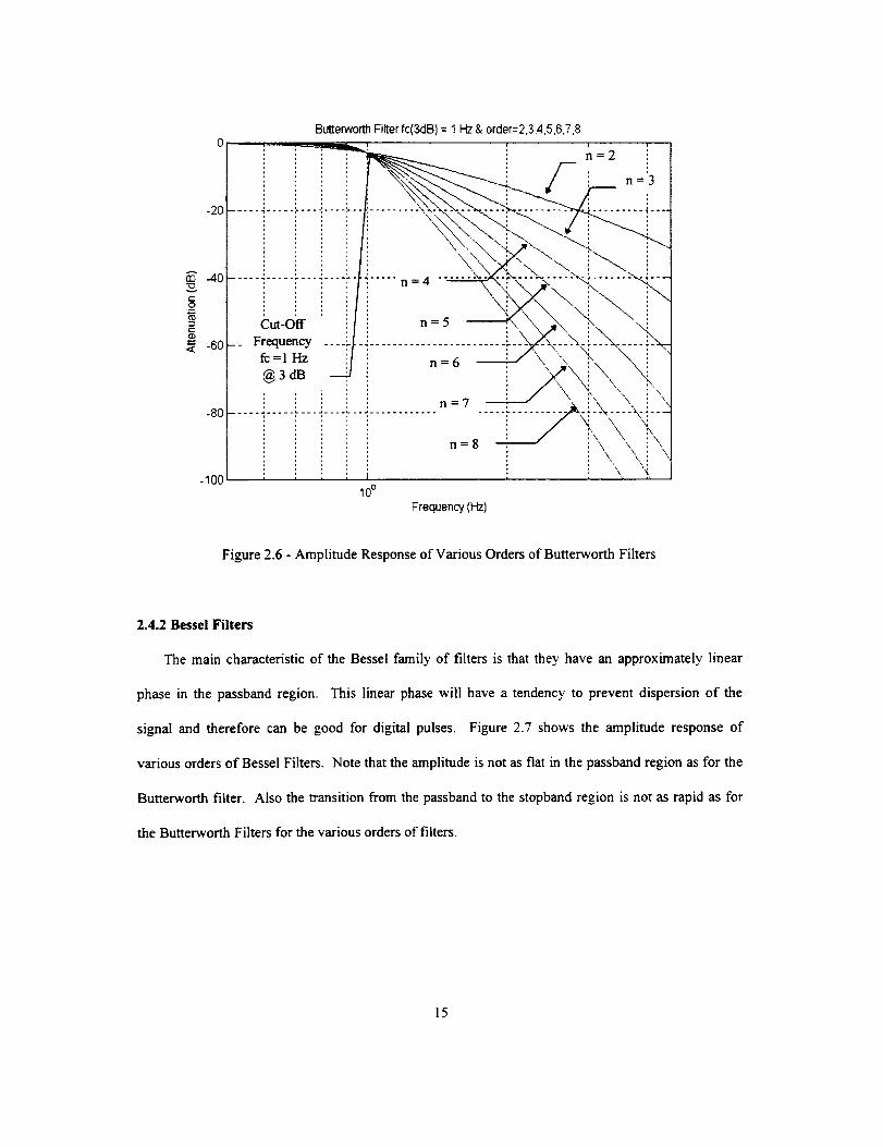
2.4.2 Bessel Filters
The main characteristic of the Bessel family of filters is that they have an approximately linear
phase in the passband region. This linear phase will have a tendency to prevent dispersion of the
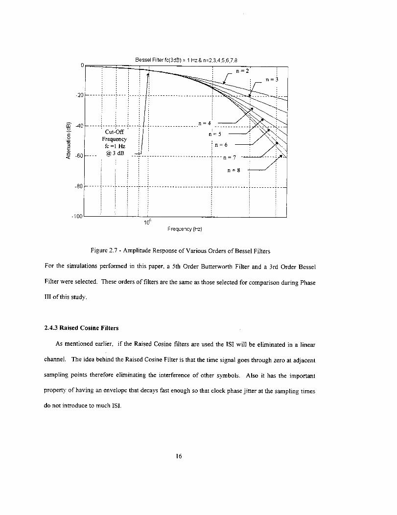
signal and therefore can be good for digital pulses. Figure 2.7 shows the amplitude response of
various orders of Bessel Filters. Note that the amplitude is not as flat in the passband region as for the
Butterworth filter. Also the transition from the passband to the stopband region is not as rapid as for
the Butterworth Filters for the various orders of filters.
15
-20
n', -40"(5
t-O
q_
_7 -60
Bessel Filter fc(3dB) = 1 Hz & n:2,3,4,5,6,7,8
i _ i i . i n=2' !
----_!_
..... .2.1........................L....o=7n=8
-80 1 ...........................................................................
-10010°
Frequency (l.-{z)
Figure 2.7 - Amplitude Response of Various Orders of Bessel Filters
For the simulations performed in this paper, a 5th Order Butterworth Filter and a 3rd Order Bessel
Filter were selected. These orders of filters are the same as those selected for comparison during Phase
III of this study.
2.4.3 Raised Cosine Filters
As mentioned earlier, if the Raised Cosine filters are used the ISI will be eliminated in a linear
channel. The idea behind the Raised Cosine Filter is that the time signal goes through zero at adjacent
sampling points therefore eliminating the interference of other symbols. Also it has the important
property, of having an envelope that decays fast enough so that clock phase jitter at the sampling times
do not introduce to much ISI.
16
The transfer function of the Raised Cosine Filter is
X(f) =
T,
T(1 - sin[(2n If2_- 7t)_,
0_
(1 -ct)o _<lfl <
2T
(1-ct) <]f[_< (1 +o.)2T 2T
(1 +or)Ifl>2T
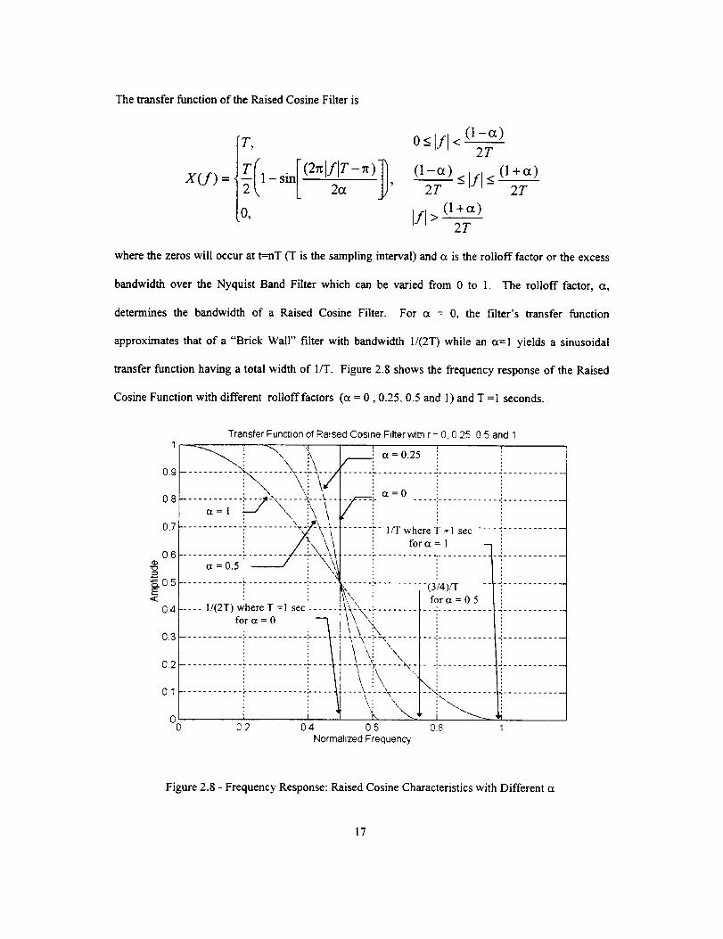
where the zeros will occur at t=nT (T is the sampling interval) and ct is the rolloff factor or the excess
bandwidth over the Nyquist Band Filter which can be varied from 0 to I. The rolloff factor, cq
determines the bandwidth of a Raised Cosine Filter. For ct = 0, the filter's transfer function
approximates that of a "Brick Wall" filter with bandwidth I/(2T) while an et=l yields a sinusoidal
transfer function having a total width of 1/T. Figure 2.8 shows the frequency response of the Raised
Cosine Function with different rolloff factors (ct = 0,0.25, 0.5 and 1) and T =1 seconds.
08
Transfer Function of Raised Cosine Filter _th r = 0,025, 05 and 1
ct =0.5
I/(2T) where T =1 sec ......forct =0
"-i'- I/T where T =1 secfor ct = 1
(3/4)/Tforct = 0.5
\
02 04 06 0.8 1Normalized Frequency
Figure 2.8 - Frequency Response: Raised Cosine Characteristics with Different ct
17
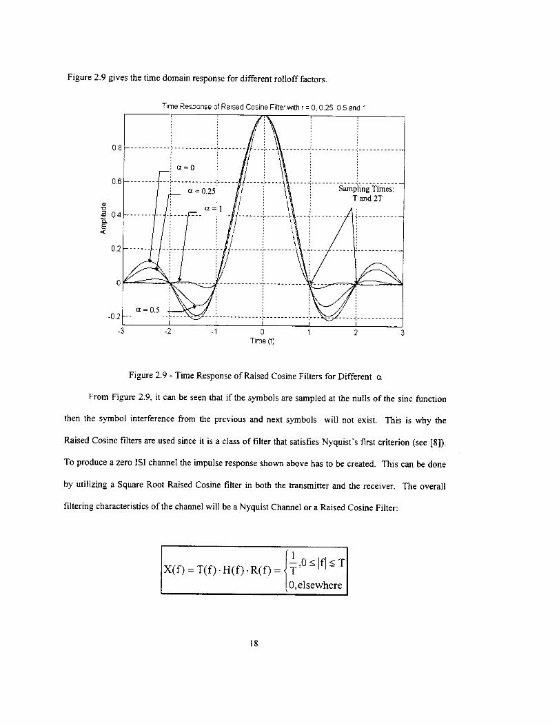
Figure2.9givesthetimedomainresponsefordifferentrollofffactors.
Time Responseof Raised Cosine Filterwith r : O,0.25, 05 and 1
08 t ........................ a=0
06
02
- -r ............ ,....
ct = 0.25
ct=l
Sampling Times:T and 2T
-1 0Time (t]
2 3
Figure 2.9 - Time Response of Raised Cosine Filters for Different et
From Figure 2.9, it can be seen that if the symbols are sampled at the nulls of the sinc function
then the symbol interference from the previous and next symbols will not exist. This is why the
Raised Cosine filters are used since it is a class of filter that satisfies Nyquist's first criterion (see [8]).
To produce a zero ISI channel the impulse response shown above has to be created. This can be done
by utilizing a Square Root Raised Cosine filter in both the transmitter and the receiver. The overall
filtering characteristics of the channel will be a Nyquist Channel or a Raised Cosine Filter:
[0,elsewhere [
18
where T(f)isthefrequencyresponseof the transmitter;
H(f) is the frequency response of the channel;
R(f) is the frequency response of the receiver; and
X(f) is the overall frequency response of the system.
If the channel has a large bandwidth compared to the transmitter and receiver frequency response
then
Ix(f) = T(f). R(f)= RC(f)]
where RC(f) is the frequency response of the Raised Cosine Filter. Thus
IT(f) = R(f) = _ = SRRC(f)]
where SRRC(f) is a Square Root Raised Cosine Filter for both the transmitter and the
receiver which maximizes the data transmission efficiency (both the transmitter and receiver are
matched). Therefore, the channel will be a Nyquist Channel (or Raised Cosine Function) with zero ISI
for optimum data detection. This does not apply for a non-linear channel as will be shown when a
non-linear device such as a Solid State Power Amplifier (SSPA) is present in the channel.
As stated in [3]: "Raised Cosine Filters were selected for evaluation because the linearity of their
phase-frequency relationship should help to eliminate the ringing found in the Butterworth filters at the
cut-off frequency. Their comparatively narrow bandwidth, combined with a smooth response, should
provide a signal which concentrates most of the data sideband energy near the main lobe significantly
attenuating the sidebands. Such filters are commonly employed to pack a multiplicity of signals in a
conf'med frequency band."
19
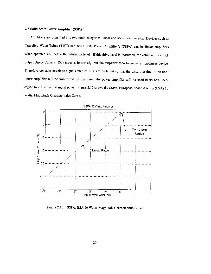
2.5 Solid State Power Amplifier (SSPA)
Amplifiers are classified into two main categories: linear and non-linear circuits. Devices such as
Traveling-Wave Tubes (TWT) and Solid State Power Amplifier's (SSPA) can be linear amplifiers
when operated well below the saturation level. If this drive level is increased, the efficiency, i.e., RF
output/Direct Current (DC) input is improved, but the amplifier then becomes a non-linear device.
Therefore constant envelope signals such as PSK are preferred so that the distortion due to the non-
linear amplifier will be minimized. In this case, the power amplifier will be used in its non-linear
region to maximize the signal power. Figure 2.10 shows the SSPA, European Space Agency (ESA) 10
Watts, Magnitude Characteristics Curve.
SSPA 10Watts Amplifier
o...........!..........i.....................i i i _.-;....... i i
......................................Region
-_0............................... _ ........ ._...............................
_-15 ................. ".Linear Region .............................a
"5 ',
o -20 ........... _: ........ ! .....................................................f,,
-25
-30-30
//
-25 -20 -15 -10 -5inputLevelPower (dB)
Figure 2.10 - SSPA, ESA I 0 Watts, Magnitude Characteristic Curve
2O
The non-linearities that occur in the nonlinear region of this amplifier will cause non-linear
distortion and Amplitude Modulation-to-Phase Modulation (AM-to-PM) and AM-to-AM conversion
effects (linear channels are channels without AM-AM and AM-PM conversions). As mentioned in
[8], the analysis of these non-linearities are very complicated.
In this study the non-linear channel will be considered (the power amplifier will be operated in its
saturation region). Even if SRRC filters are used for the transmitter and receiver, ISI-free sample
points no longer exist because of the distortion introduced by the system. This will be shown and
discussed in Chapter 3 - 8PSK Simulations. Thus, the objective of this study is not only to find a
bandwidth efficient communications system which can increase frequency band-utilization, but also, to
identify an implementation that can be realized.
NMSU used the SSPA model for their simulation which is based upon specifications provided by
the European Space Agency (ESA) for their 10 Watts, solid state, S-band power amplifier. This power
amplifier was selected since all the simulations performed in Phases II and II1 (refer to [3], [4]) were
done using this amplifier.
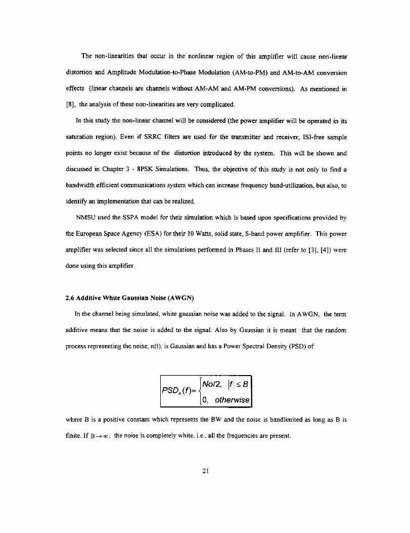
2.6 Additive White Gaussian Noise (AWGN)
In the channel being simulated, white gaussian noise was added to the signal. In AWGN, the term
additive means that the noise is added to the signal. Also by Gaussian it is meant that the random
process representing the noise, n(t), is Gaussian and has a Power Spectral Density (PSD) of
f
JNol2, f < BPSD_ (f)= 1
LO, otherwise
where B is a positive constant which represents the BW and the noise is bandlimited as long as B is
finite. If B--_ oc, the noise is completely white, i.e., all the frequencies are present.
21
Gaussianprocessesgiveagoodapproximationof naturallyoccurringbehaviors.Additionofthe
noise,n(t),willgiver(t)=s(t)+n(t)where
- n(t)istheAWGNwithvariance= o_2=No/2andmean=m,=0;
- s(t)isthesignal;and
- r(t)istheresultingsignalwiththenoiseadded.
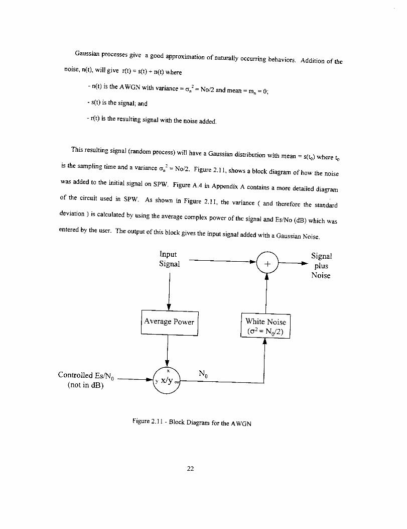
This resulting signal (random process) will have a Gaussian distribution with mean = S(to) where to
is the sampling time and a variance or, 2 = No/2. Figure 2.11, shows a block diagram of how the noise
was added to the initial signal on SPW. Figure A.4 in Appendix A contains a more detailed diagram
of the circuit used in SPW. As shown in Figure 2.1 I, the variance ( and therefore the standard
deviation ) is calculated by using the average complex power of the signal and Es/No (dB) which was
entered by the user. The output of this block gives the input signal added with a Gaussian Noise.
Controlled Es/N 0
(not in dB)
Input
Signal
r
IAverage P°wer I I (o.Wh2il=eNN_i2_e I
N OT
v
Signal
plus
Noise
Figure 2.11 - Block Diagram for the AWGN
22
Inour simulations, a variation of the integrate-and-dump filter was used. This was possible since
the digital signaling format has a rectangular bit shape. For the integrate-and-dump filter, the digital
input signal plus the noise is integrated over one symbol period T and the output of the integrator is
dumped at the end of the symbol period which is the value that is required. Therefore for proper
operation of this optimum filter, an external clocking signal called bit sync is required.
24
Chapter 3
8PSK SIMULATIONS
3.1 Simulation Procedures
To simulate the non linear satellite link, a Signal Processing Worksystem (SPW) which is a
COMDISCO simulation software was utilized on a SUN Sparc Station 10 and HP Model 715/100
Unix Station. The following diagram shows the different blocks that were simulated on the
workstation.
i
DATA SOURCE
BASEBAND t
SPECTRUM
SHAPING
- Butterworth
5th Order
- Bessel 3rd Order
- SRRC
(sampled data)
r .......... _ .......
i
2nd
HARMONICFILTER
- Butterworth
4th Order AWGN
AMPLIFIER CHANNEL
ERROR t
RATE
ESTIMATORDELAY
&
PHASE
METER
MATCHED
FILTER
ERROR RATE SYNCHRONIZER
- Sliding
Integrator
RECEIVER
r
Figure 3.1 - Simulation Block Diagram
25
FirstaDataSourceorModulatorwasusedtoproducethe 8PSKsignal.Thedatasourcealso
containedablockthatcouldproducedataasymmetryonthedata.All simulationswereproducedat
basebandusingthecomplexenvelopesignalrepresentation.Theresultsdonotvaryif thesimulations
aredoneinbasebandorpassband.Theadvantageof goingto basebandis thecomputerexecution
time,i.e.,it takeslongertosimulateatpassbandsincethesamplingfrequencymustbeatleasttwice
theNyquistrate.Thenextblockafterthemodulatoristhebasebandspectrumshapingfilter.Thethree
typesoffiltersthatwereusedforthesesimulationswere5thOrderButterworth,3rdOrderBessel,and
f'mallySquareRootRaisedCosine(SRRC)withSampledDataandRoll-Offfactorsof0.25,0.5and1.
ThenextblocksincludetheSSPA,abandlimitingfilterandthenoise(channel).Simulationswere
performedusingtheSSPAatthesaturationlevelto maximizethepower.Simulationsatsaturation
werethenfollowedbysimulationswiththeSSPAbackedoff by-10 riB. This amplifier was followed
by a 2rid Harmonic filter (4th Order Butterworth with a bandwidth of +_ 20Rs) which reduces the
interference between different channels. This bandlimiting filter is followed by the variable AWGN
(variable to be able to control the Es/No values).
These blocks were followed by the Receiver, Symbol Synchronizer and finally the Error Estimator.
A matched filter (sliding integrator) was used as the receiver for the Butterworth and Bessel Filters.
The matched filter was matched to the NRZ-L baseband data. For the SRRC, the receiver was also a
SRRC to minimize the ISI. The SRRC will minimize the ISI and the matched filter is an optimum
filter which optimizes the Signal-to-Noise ratio (SNR). The synchronizer that was used consisted in a
Delay and Phase Meter that would correlate, as best as it could, the initial data with the data that went
through the channel.
After these two signals went through the phase and delay meter, the initial data were delayed to be
synchronized with the distorted data (the delay between the initial and distorted data were caused by
the filters). After the data were synchronized (the best correlation was found), an Error Rate
Estimator was used to measure the differences in symbols and calculate the Symbol Error Rate (SER).
26
WhenthePowerContainmentswereneededaSpectrumAnalyzerfromSPWwasplacedafterthe
2ndHarmonicFilter.
ThefollowingvariablesandsystemswereimplementedinSPWforthesimulations:
(a)- SPWSimulationVariables:
i - Bitrate= I bps(Rs=symbolrate=(1/3)symbols/sfor8PSK)
ii - Sample Rate = fs = 16 samples/sec
iii - Data: NRZ-L
iv - Carrier Frequency = 0Hz (Baseband Simulations)
(b) - Transmitting System:
i - Data Generator: Ideal and Non-ldeal Data:
- data asymmetry = 2%
- data imbalance = 0.45
ii - Baseband filters (do not include resistive and reactive losses):
- Butterworth 5th Order (BT =1,2,3);
- Bessel 3rd Order (BT=l,2,3)
- SRRC (ct =0.25, 0.5 and 1) with 256 taps
Note BT represents the product of the bandwidth (3 dB single-sided)
with the symbol time; thus if BT = I it means that
B = (I/3) since T = (l/Rs) = (1/(1/3)) = 3.
- Also 256 taps where chosen because we will have:
(256 taps/16 samples/sec)/2 = 8 symbols interfering with
the one being sampled. It was noted that using more
taps on the Infinite Impulse Response (IIR) filter did not
affect the output.
27
iii - PowerAmplifierbasedon:
- European Space Agency (ESA) 10-Watt
Solid State Power Amplifier (SSPA);
- 4th Order Butterworth (cutoff at + 20 Rs) - 2rid Harmonic Filter
- protects user's of other bands.
(c) - Receiving System:
i - Matched Filter: Sliding Integrator
ii - Delay and Phase Meter (synchronization); and
iii - Error Rate Estimator.
The following simulations were performed with the system described above
(a) - Power Containment and Spurious Emissions;
(b) - End-to-End System Performance " Symbol Error Rate (SER); and
(c) - Non-Constant Envelope Simulations (a variation of the circuit shown in Figure 3.1 was
utilized).
3.2 Power Containment and Spurious Emissions Simulations
Table 3.1, summarizes the simulations performed for 8PSK ( the numbers in parenthesis, (1) etc.
indicate individual runs that were performed):
28
iiiiiflllllll
_ +1 +1 _ _ _ _ +1 _ +1 _ _ _ _ +t _ +i +1 _ _ _ _ +1 __l_lllll, It It II II II ,l I, II II
•- ,,. _ -_ -_ -_ _ -__= 2: _:z -z =_z -z _=z -z z -z z -z z
29
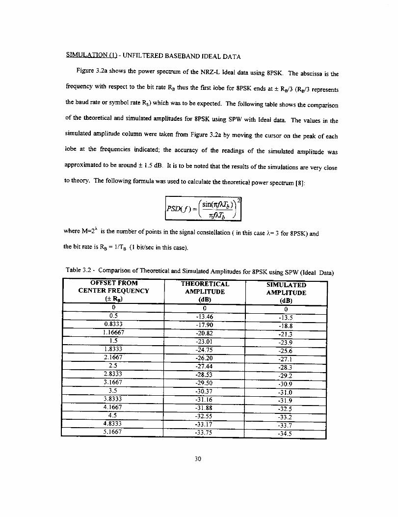
SIMULATION (I) - UNFILTERED BASEBAND IDEAL DATA
Figure 3.2a shows the power spectrum of the NRZ-L Ideal data using 8PSK. The abscissa is the
frequency with respect to the bit rate RB thus the first lobe for 8PSK ends at +_Re/3 (Re/3 represents
the baud rate or symbol rate Rs) which was to be expected. The following table shows the comparison
of the theoretical and simulated amplitudes for 8PSK using SPW with ldeal data. The values in the
simulated amplitude column were taken from Figure 3.2a by moving the cursor on the peak of each
lobe at the frequencies indicated; the accuracy of the readings of the simulated amplitude was
approximated to be around + 1.5 dB. It is to be noted that the results of the simulations are very close
to theory. The following formula was used to calculate the theoretical power spectrum [8]:
PSD(f)=\ rcfLTb J
where M=2 x is the number of points in the signal constellation ( in this case _.= 3 for 8PSK) and
the bit rate is RB = 1/TB (1 bit/sec in this case).
Table 3.2 - Comparison of Theoretical and Simulated Amplitudes for 8PSK using SPW (Ideal Data)
OFFSET FROM
CENTER FREQUENCY
(+ Re)
THEORETICAL
AMPLITUDE
(dB)
0
'SIMULATED
AMPLITUDE
(dB)
0.5 -13.46 -13.5
0.8333 - 17.90 - 18.8
1.16667 -20.82 -21.3
1.5 -23.01 -23.9
1.8333 -24.75 -25.6
2.1667" -26.20 -27.1
2.5 -27.44 -28.3
2.8333 -28.53 -29.2
3.1667 -29.50 -30.9
3.5 -30.37 -31.0
3.8333 -31.16 -31.9
4.1667 -31.88 -32.5
4.5 -32.55 -33.2
4.8333 -33.17 -33.7
5.1667 -33.75 -34.5
30
+1
÷t
..C3
O0 0
o D.c,_
0
i
t_
o
3]
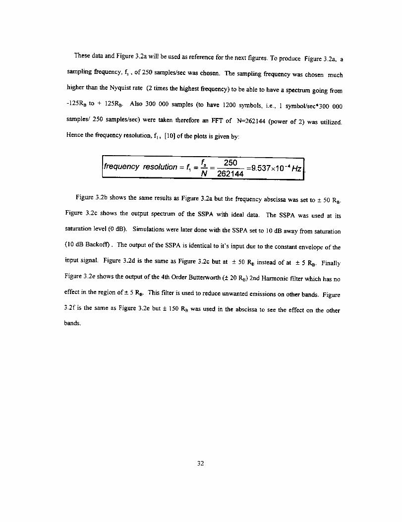
These data and Figure 3.2a will be used as reference for the next figures. To produce Figure 3.2a, a
sampling frequency, fs, of 250 samples/sec was chosen. The sampling frequency was chosen much
higher than the Nyquist rate (2 times the highest frequency) to be able to have a spec_m going from
-125R a to + 125RB. Also 300 000 samples (to have 1200 symbols, i.e., 1 symbol/sec*300 000
samples/250 samples/sec) were taken therefore an FFT of N=262144 (power of 2) was utilized.
Hence the frequency resolution, fl, [10] of the plots is given by:
_f,frequency resolution = f_ N _ 250 =9.537x10_4Hz]262144 ,, "
Figure 3.2b shows the same results as Figure 3.2a but the frequency abscissa was set to + 50 R s.
Figure 3.2c shows the output spectrum of the SSPA with ideal data. The SSPA was used at its
saturation level (0 dB). Simulations were later done with the SSPA set to i0 dB away from saturation
(10 dB Backoff). The output of the SSPA is identical to it's input due to the constant envelope of the
input signal. Figure 3.2d is the same as Figure 3.2c but at + 50 Rs instead of at _+5 Ra. Finally
Figure 3.2e shows the output of the 4th Order Butterworth (4- 20 Ra) 2nd Harmonic filter which has no
effect in the region of+_ 5 Rs. This filter is used to reduce unwanted emissions on other bands. Figure
3.2f is the same as Figure 3.2e but _+ 150 RB was used in the abscissa to see the effect on the other
bands.
32
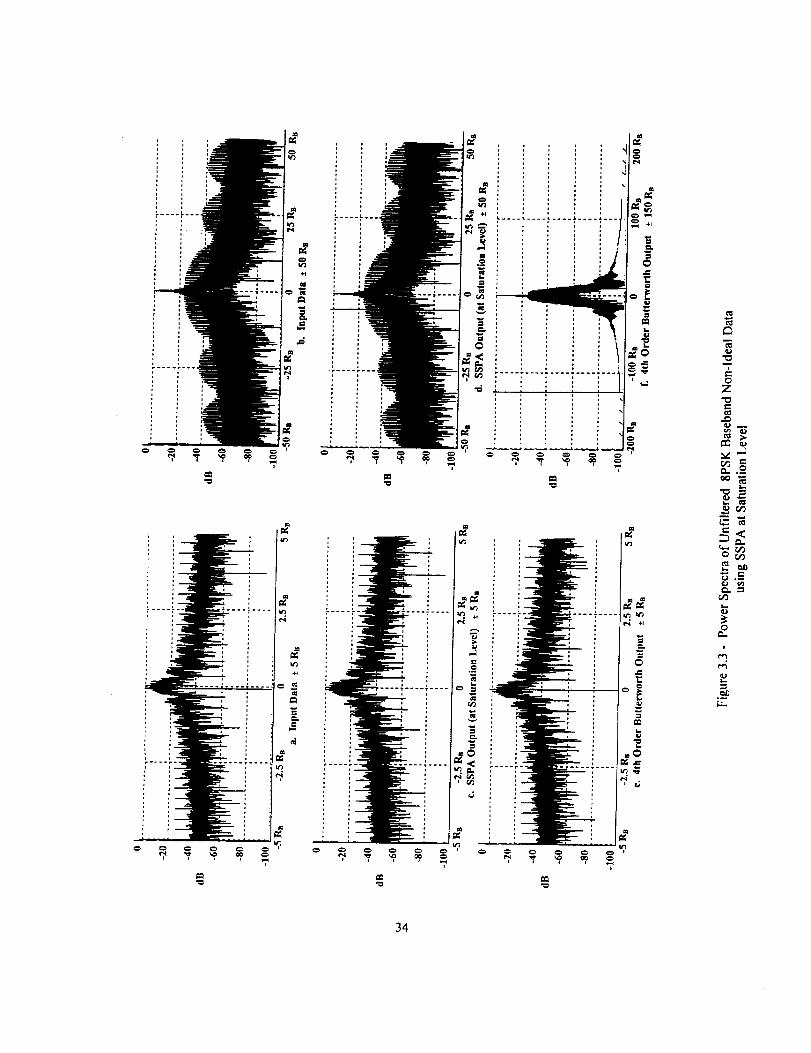
SIMULATION (2) - UNFILTERED BASEBAND NON-IDEAL DATA
For this simulation, the data symmetry was set to 2% and the probability of zero = 0.45. Figure
3.3a shows the unfiltered baseband data (Non-Ideal Data) at the output of the 8PSK modulator. The
presence of spurs at approximately f = n*Rs (where n=0,1,2..) are due to the probability of zero which
is not equiprobable, i.e., equal to 0.5, and to the data asymmetry. The spurs are more evident in Figure
3.3b.
Figure 3.3c and 3.3d show the output of the SSPA (at saturation level) and as mentioned earlier
there is no effect or difference with the input data since it is a constant envelope signal (no spectrum
shaping filter present) going through the amplifier. Figure 3.3e and 3.3f show the output of the 4th
Order Butterworth filter at _+5R a and _+150R B.
Simulations (1) and (2) will be used as references for the spectrum shaping filter simulations.
.9.9
0
Z
4,) N
ee_ _
.0..
0
i
.__t,.
34
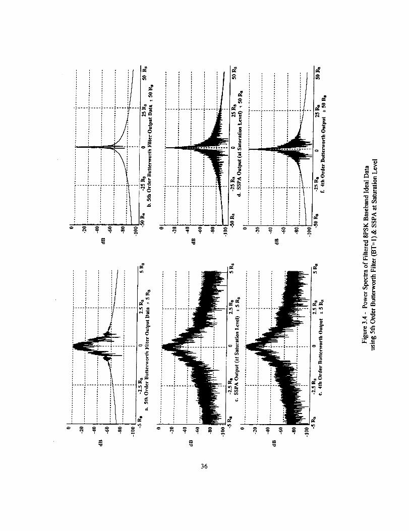
SIMULATION (3) AND (4) - 5TH ORDER BUTTERWORTH FILTERED BASEBAND DATA
(IDEAL AND NON-IDEAL DATA)
For this simulation, the sampling frequency (fs) was set to 250 samples/sec, the symbol rate (Rs) =
(1/3) symbols/sec, the number of samples set to 300 000 and the number of FFT points (N) = 524 288.
The BT product was set to 1 thus the bandwidth B = Rs and T = I/R s which is the symbol interval.
For the non-ideal data, the data asymmetry was again set to 2% and the probability of zero was set to
0.45.
Figure 3.4a and 3.5a show the result of the baseband data going through the 5th Order Butterworth
Filter for ideal and non-ideal data, respectively. Note that at approximately + 2R s the filter attenuates
the data sidebands by approximately 40 dB. Figures 3.4c and 3.5c show the output of the SSPA for
the ideal and non-ideal data. Note that due to the non-constant envelope of the data (since some
spectrum shaping was performed), the output of the SSPA is quite different from Figure 3.2c and
3.3c. In fact, it seems like the SSPA is trying to recreate the sidelobes that were attenuated by the
filter. Also, the spurious emissions encountered in Figure 3.3d for the non-ideal case are not present or
are fairly attenuated. In [3] for PCM/PM/NRZ it was reported that the Butterworth Baseband Filter
introduced large in-band spurious emissions which does not seem to appear here. Comparing Figures
3.4d and 3.5d seems to demonstrate that there is no difference at the output of the SSPA for ideal and
non-ideal data using the Butterworth Filter, compared to the plots with no filter and non-ideal data in
Figures 3.2d and 3.3d where the spurs are obvious. Figures 3.4e/3.4f and 3.5e/3.5f show the output of
the 4th order Butterworth with ideal and non-ideal data.
If the amount of attenuation from baseband filtering is examined by comparing with Figures
3.2c/3.2d and 3.3c/3.3d with 3.4c/3.4d and 3.5c/3.5d (Butterworth Filter), it can be seen that at
approximately + 0.5RB, the Butterworth filter attenuates the sidebands by approximately 23 dB. At
approximately _+2.5 R B, the attenuation is around 50dB below the peak of the main lobe, placing the
absolute level of the sidebands under 50 dB after this point.
35
1:
m
36
0
zg,
_m
[.i. -,=.
K_
i
d_
37
Tables 3.3 and 3.4, at the end of this Chapter, summarize the attenuation spectrum levels relative
to the fin-st data sideband for Ideal and Non-Ideal data. This information about sideband attenuation
will be important when discussing the utilization ratio (p) and band utilization in a latter section.
SIMULATION (5) AND (6) - 3 rd ORDER BESSEL FILTERED BASEBAND DATA
(IDEAL AND NON-IDEAL DATA)
Again these two simulations used the same parameters as those discussed for the 5th Order
Butterworth filter. In the case of the Bessel filter the effect of in-band spurious emissions are more
present and more evident than for the Butterworth filter as shown in Figure 3.7a compared to Figure
3.6a. The output of the SSPA (Figures 3.6c/3.6d and 3.7c/3.7d for ideal and non-ideal data
respectively) show some small spurs emissions caused by the non-ideal data.
With respect to the sideband attenuation, the values of attenuation for the Bessel (3rd Order) are
comparable to the 5th Order Butterworth filter (see Tables 3.3 and 3.4).
38
°
.................... ÷i
i
°_
I. Q_,
o _
, ©
39
t
...............]....i
o___a_
o :
z_
c= _"
4O
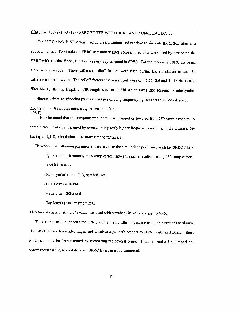
SIMULATION (7) TO (12) - SRRC FILTER WITH IDEAL AND NON-IDEAL DATA
The SRRC block in SPW was used as the transmitter and receiver to simulate the SRRC filter as a
spectntm filter. To simulate a SRRC transmitter filter non-sampled data were used by cascading the
SRRC with a 1/sinc filter ( function already implemented in SPW). For the receiving SRRC no 1/sinc
filter was cascaded. Three different rolloff factors were used during the simulation to see the
difference in bandwidth. The rolloff factors that were used were et = 0.25, 0.5 and 1. In the SRRC
filter block, the tap length or FIR length was set to 256 which takes into account 8 intersymbol
interferences from neighboring pulses since the sampling frequency, fs, was set to 16 samples/sec:
= 8 samples interfering before and after.
2*(fs)It is to be noted that the sampling frequency was changed or lowered from 250 samples/see to 16
samples/sec. Nothing is gained by oversampling (only higher frequencies are seen in the graphs). By
having a high fs, simulations take more time to terminate.
Therefore, the following parameters were used for the simulations performed with the SRRC filters:
- f_ = sampling frequency = 16 samples/sec (gives the same results as using 250 samples/see
and it is faster)
- Rs -- symbol rate = (1/3) symbols/sec;
- FFT Points = 16384;
- # samples = 20K; and
- Tap length (FIR length) = 256.
Also for data asymmetry a 2% value was used with a probability of zero equal to 0.45.
Thus in this section, spectra for SRRC with a l/sinc filter in cascade at the transmitter are shown.
The SRRC filters have advantages and disadvantages with respect to Butterworth and Bessel filters
which can only be demonstrated by comparing the several types. Thus, to make the comparison,
power spectra using several different SRRC filters must be examined.
41
Square Root Raised Cosine Filter (a = 0.25)
Comparing Figures 3.8a and 3.9a of a SRRC filter with a roll-off factor of ct = 0.25 with Figures
3.4a and 3.5a for Butterworth and Figures 3.6a and 3.7a for Bessel Filters, it is immediately noted that
the SRRC filters offers a significant advantage over both of the Butterworth and Bessel filters (BT=l
for both these filters). The spectrum is narrower, better defined and cleaner than the spectra for other
filter types. On the other hand, the attenuation is less than that for the Butterworth or Bessel filters at
high Ra (-_ - 20 RB) as indicated in Tables 3.3 and 3.4. In-band spurious emissions are absent, even
for non-ideal data. This is the narrowest bandwidth SRRC filter that is considered in this study.
Outputs from the power amplifier (see Figures 3.8b/3.8c and 3.9b/3.9c for ideal and non-ideal data
respectively) shows that the nonlinearity (and non constant-envelope signal going in) in the SSPA
causes an increase in amplitude in the l to 4 R B region. Finally Figures 3.8d/3.Se and 3.9d/3.9e shows
the output of the 4th Order Butterworth Filter. Note how the attenuation remains fairly constant around
-7RB with a value of approximately -68 dB.
42
e_c_
o_ e_l
_-' iN
_o
_l rs_
43
t_
t_L _S_C_ r_
_ o_
L_ L_
t _0
L_
LL
44
Square Root Raised Cosine Filter (a = 0.5)
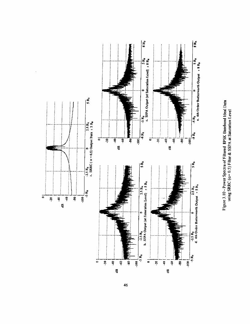
Similar power spectrum plots are found for the case ofa = 0.5 (Figures 3.10a and 3.1 la) compared
to Figures 3.8a and 3.9a. The bandwidth is slightly wider for this case (_t = 0.5). Nonetheless as with
SRRC (a = 0.25 ), the transmitted power spectrum (Figures 3.10e or 3.1 le for ideal and non-ideal
data respectively) is smooth and the absence of in-band spurious emissions is obvious, even for non-
ideal dam But again, the attenuation produced by the Butterworth or Bessel Filter is much superior at
higher frequencies than the SRRC (refer to Tables 3.3 and 3.4). Therefore since there appears to be no
significant difference in the spectra between the SRRC with ct = 0.25 and a = 0.5, the selection must
depend upon other factors such as ISI, implementation complexity, etc.
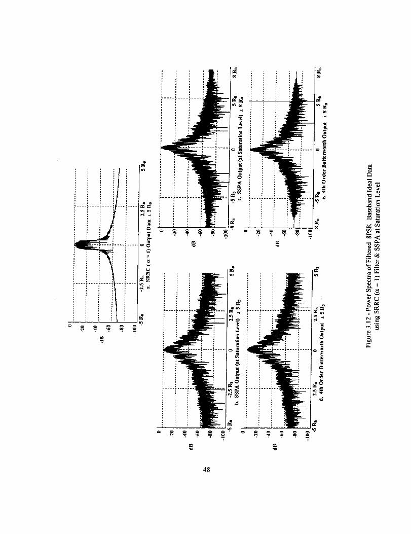
Square Root Raised Cosine Filter (a = I)
A SRRC filter with an a = 1 has a larger bandwidth than filters with smaller values of co, therefore
the baseband data spectrum using ideal and non-ideal data (Figures 3.12a and 3.13a) are wider (than
for a = 0.25 and ct = 0.5). Also, it is to be noted in Figures 3.12b/3.12c and 3.13b!3.13c, the higher
order sidebands ( 2nd, 3rd, .. lobes) are more visible in contrast to the other SRRC filters.
Nonetheless, again at the power amplifier's output (Figures 3.12b/3.12c or 3.13b/3.13 c for ideal
and non-ideal data respectively), the spectrum is characterized by a smooth roll-off with no-in band
spurious emissions evident. Due to this filter's wider bandwidth, the attenuation is slightly less than
that for filters with smaller values of ct especially with the non-ideal data (refer to Tables 3.3 and 3.4).
45
k .... _ .... L .... _ .......
-i ....
_'!_J__I_i....i....i.......__+_'
i
!
t,.-. +t,...
,.m+_
+,,,...-,c,_.,
_<_
_'_
=.__
46

c_
r_
L_
Z _
o_ _
o__ ._
_0
47
: =
r_.__
oo<:c_
r__.)
L;. _-
a= _'-
r_i
48

r_
z_
c_
0 _
_ el)
i r-o_
_0o_
49
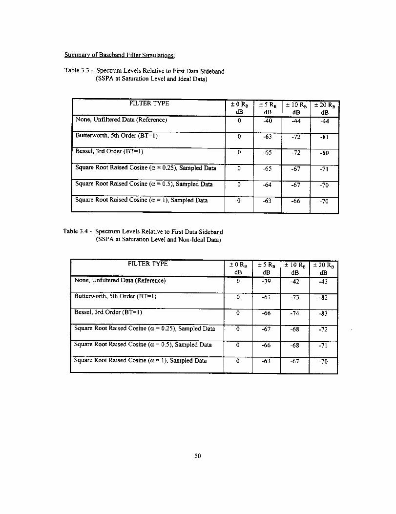
Summary_ of Baseband Filter Simulations:
Table 3.3 - Spectrum Levels Relative to First Data Sideband
(SSPA at Saturation Level and Ideal Data)
FILTER TYPE
None, Unfiltered Data (Reference)
-0 RB + 5 R B - 10 RBdB dB
-40 -44
-63 -72
dB
0
0 -64
0 -63
_+20 R B
dB
-44
Butterworth, 5th Order (BT=I) 0 -81
Bessel, 3rd Order (BT=I) 0 -65 -72 -80
Square Root Raised Cosine (a = 0.25), Sampled Data 0 -65 -67 -71
Square Root Raised Cosine (a = 0.5), Sampled Data -67 -70
Square Root Raised Cosine (_ = 1), Sampled Data -66 -70
Table 3.4 - Spectrum Levels Relative to First Data Sideband
(SSPA at Saturation Level and Non-Ideal Data)
FILTER TYPE
None, Unfiltered Data (Reference)
+ORBdB
0
+5 R adB
-39
_+ 10R BdB
-42
+ 20 RadB
-43
Butterworth, 5th Order (BT= 1) 0 -63 -73 -82
Bessel, 3rd Order (BT=I) 0 -66 -74 -83
Square Root Raised Cosine (ct = 0.25), Sampled Data 0 -67 -68 -72
Square Root Raised Cosine (a = 0.5), Sampled Data 0 -66 -68 -71
Square Root Raised Cosine (ct = I ), Sampled Data 0 -63 -67 -70
50
POWER SPECTRA FOR NON-FILTERED AND FILTERED 8 PSK
WITH SSPA BACKED OFF FROM SATURATION
All of the previous simulations were repeated for the SSPA backed off from saturation by 10 dB, so
that it is operating in the linear region. Results of these simulations are given in Figures 3.14 to 3.25.
Since the system is operating in the linear region, the power spectra plots remain the same through the
SSPA, and the 2rid Harmonic Butterworth filter.
51
i
J:Q,-j
w
o
i
..... F.... ,'-'
O3
N
_S
_0 C_
8. "_4_
m
_ r-
!
_0
52
53
oZ
e-
_<
!
_t
r_
EL _
54
, • i |
i
,,m c_
._<
mm
r_
°_la.,c,,,., ,¢,:-
C_ ,.-
c_ t:
, ©
I,. r-'
55
iiiiJi
| iQ i
! |o
, ir .... r .... r .... T .......
u
r
m
:l
F_
P4
r_ ÷l
4J
qJ
AJ
m
, ©
56
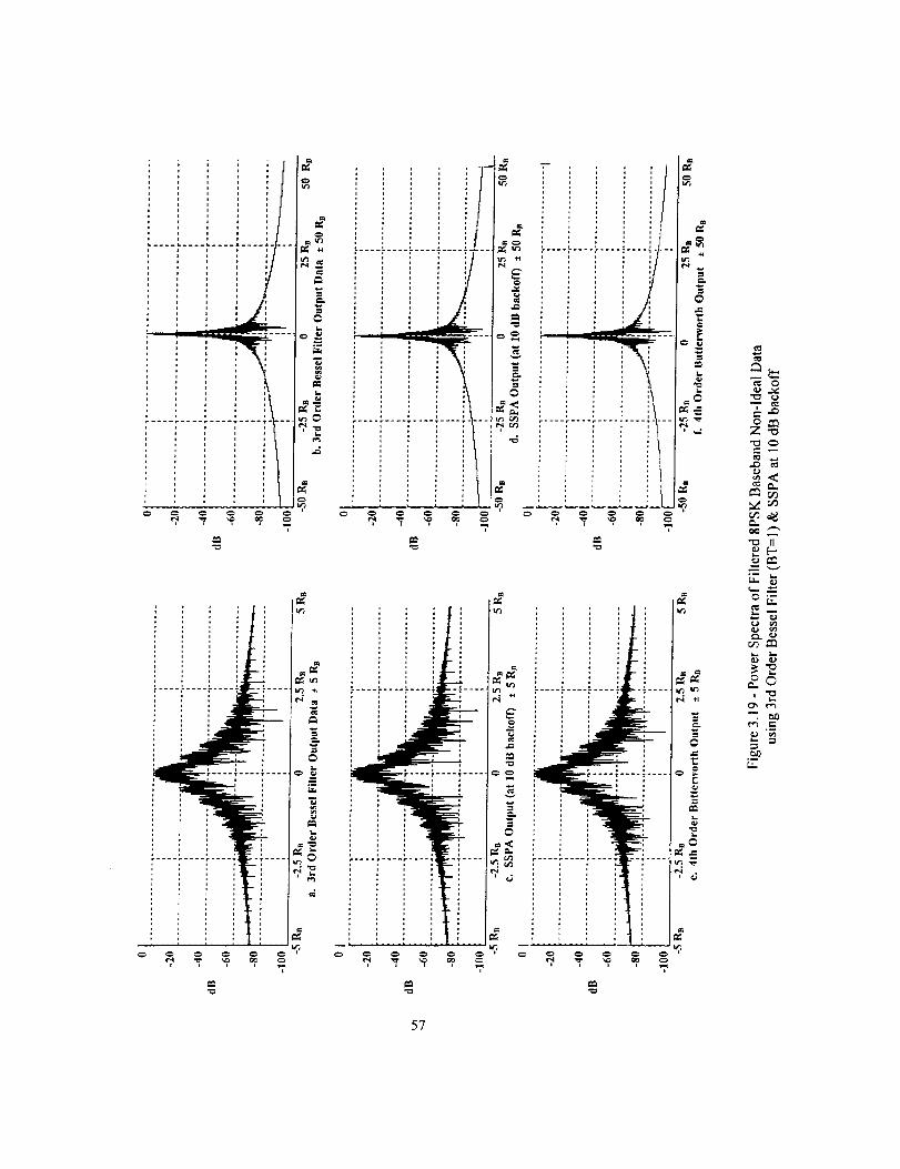
g
: :Ju
' :r|
r .... r .... r .... T .... _°
Jj
I
.d
-F-"
I
f
.... r .... P .... T .... T-L--
',
+_
_ if
° ii-,,
o
t_
,- m
e_
_o
_ e..,
57
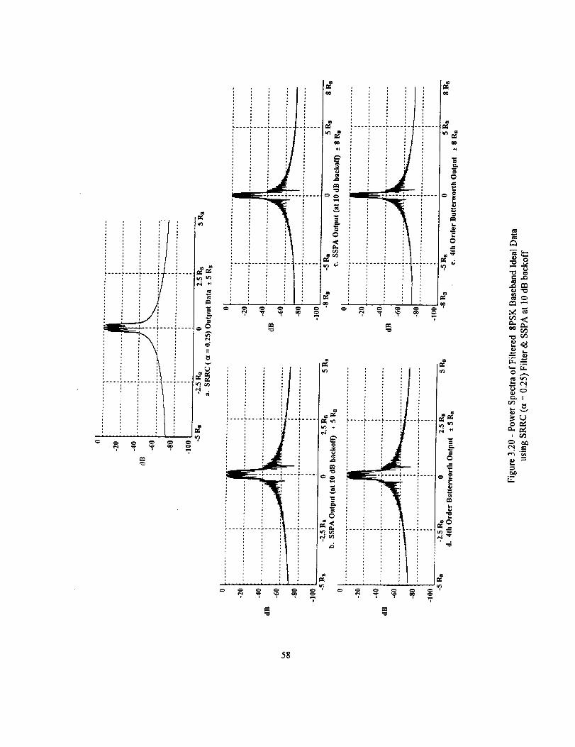
..
c_ _,c_
Lt_ k_
r_ ÷P
_f
_s
f'ii !....!....!....!...........................fl
c_
! i i i _i i i J
c_
el)mr_
iiifO_l _ C_ I c_ _ _:_
O0
ml_P
°i
"_ t_
c_
o_
°_
U_
_ r_
._ =mm_
58
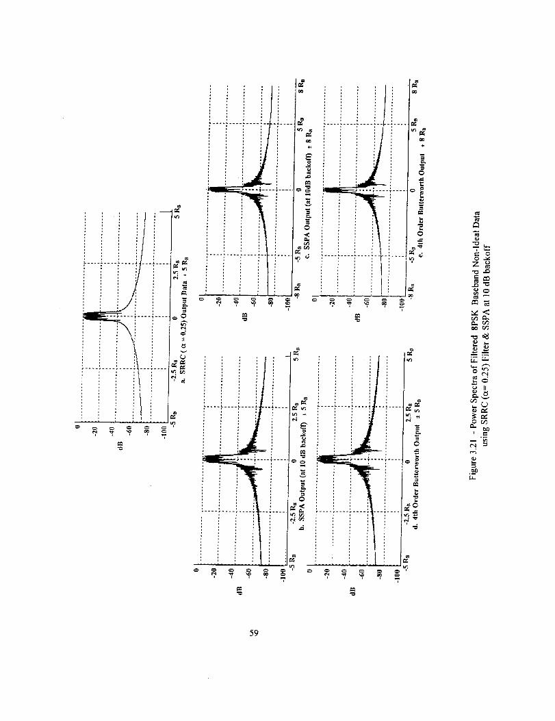
0
i/: .... : .... _.... _t.._ .... I_
, , , , @{ i i :
r .... _.... t .....: , , , ._
, , ', _._
: : : : _m
: : ', : M
i ....
r_
0
m_
c/) _-
oo c_
ca PI
0 caO
.mL_
59
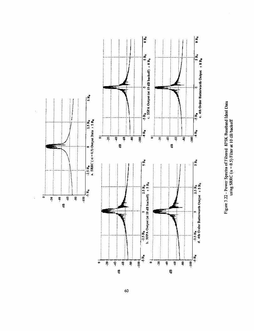
oiiiiii!Ii'T
ille_
II
---..... _ -_-....1...._....
...............:.... a _...._....F.... =T
#i#i i'......
t. ii1 _
: : : _ i i !', _ : c_ , , ,
i i i i _-_,:..... [.... 1 __.... i__ .;....
_! , ,
. -, . ._,
rm
c_
°_
c_ II
.-I
6O
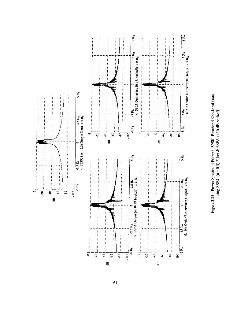
ii'-i .....
e,l
_J
z_
mm
_LT.
_-" II
°_
l"q
o
°_LT..
61

ii
..........i....it'!....
o_
0
r...
_m
,_-.E• ::_
m
62
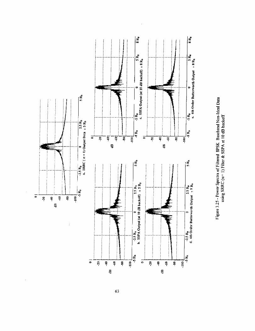
f_QO
Q. Q.Qo
G_
°_
!
Q.
6_
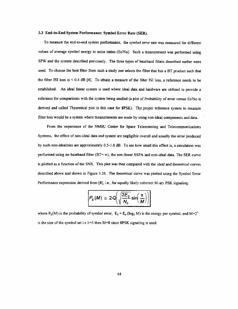
3.3 End-to-End System Performance: Symbol Error Rate (SER).
To measure the end-to-end system performance, the symbol error rate was measured for different
values of average symbol energy to noise ratios (EsfNo). Such a measurement was performed using
SPW and the system described previously. The three types of baseband filters described earlier were
used. To choose the best filter from such a study one selects the filter that has a BT product such that
the filter ISI loss is < 0.4 dB [4]. To obtain a measure of the filter ISI loss, a reference needs to be
established. An ideal linear system is used where ideal data and hardware are utilized to provide a
reference for comparisons with the system being studied (a plot of Probability of error versus EsfNo is
derived and called Theoretical plot in this case for 8PSK). The proper reference system to measure
filter loss would be a system where measurements are made by using non-ideal components and data.
From the experience of the NMSU Center for Space Telemetering and Telecommunications
Systems, the effect of non-ideal data and system are negligible overall and usually the error produced
by such non-idealities are approximately 0.5-1.0 dB. To see how small this effect is, a simulation was
performed using no baseband filter (BT = _), the non-linear SSPA and non-ideal data. The SER curve
is plotted as a function of the SNR. This plot was then compared with the ideal and theoretical curves
described above and shown in Figure 3.26. The theoretical curve was plotted using the Symbol Error
Performance expression derived from [8], i.e., for equally likely coherent M-ary PSK signaling:
\_ N o \M)
where PE(M) is the probability of symbol error, Es = E b (log_, M) is the energy per symbol, and M=2 z
is the size of the symbol set i.e _.=3 then M=8 since 8PSK signaling is used.
64
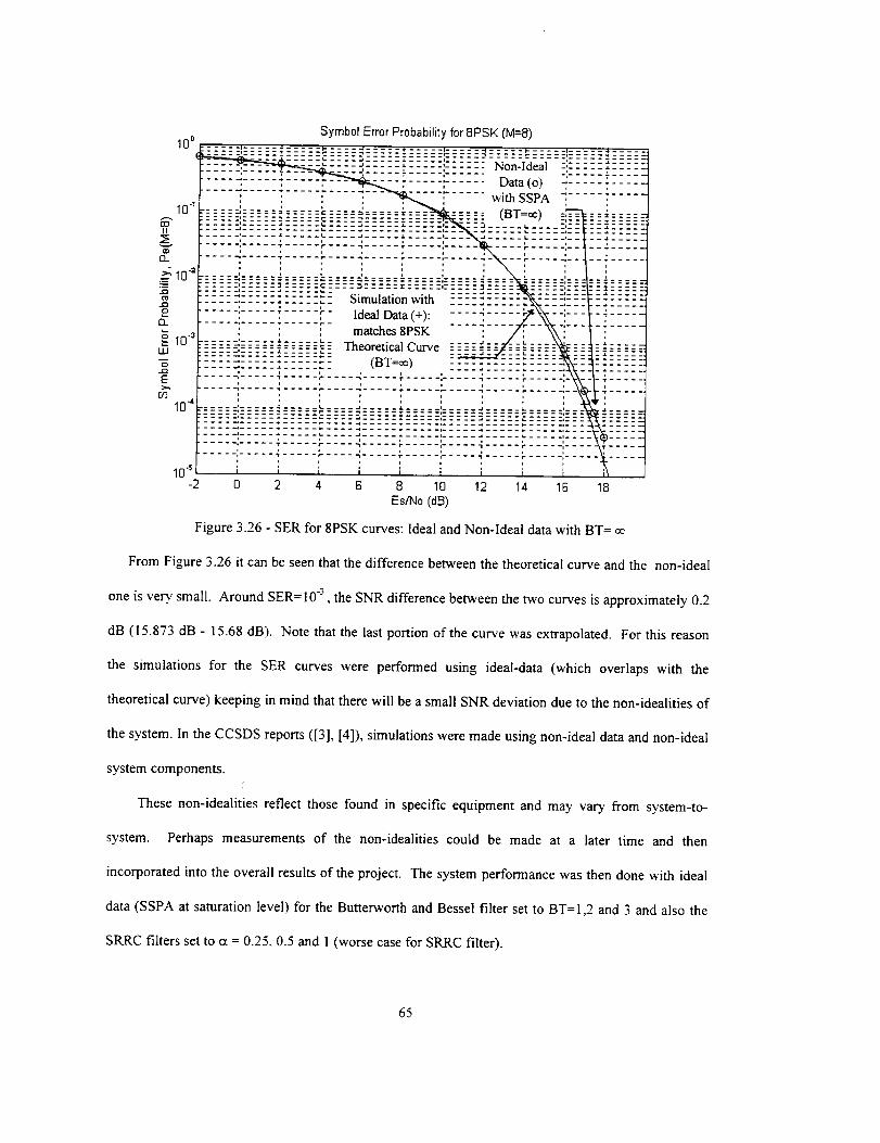
-2
Symbol Error Probability for 8PSK (M=8)
..... "-3 ..... ....... _............. ,...... Non-Ideal..... : ..... - ........ " ..... - ..... :...................... Data (o).... 2 ..... " ..... " .......
,, ..... with SSPA
:=:..... -; ..... ='.... =_...... = --.= (BT=oo)....... - _-- -.;,__-__-__-,:__-___-_-,_-__-- _.___- __. ,. ........... , ..... .t ..... t. .... .a ..... J. ..... ,_ _ _ t. ..... ,_ _
- -',- - - 4 ..... ' .... '- - - ' ..... '.- - -' - -..... e- "n -- r -- r
..... ;..... . ..... " .... 4 ..... " ..... ',..... , " ..... 1- -
' L ..... '--
___::-.:--',-:':'-----.-:--'-=--':::=:::::_¢ =::=::,::=::_::= .........Simulation with ..........
Ideal Data (+): .... .matches 8PSK
Theoretical Curve ___ ..... ----i_------_(BT=oo) - _-.- : : ..........
•_ -I- ..... '=..... -I ..... r ....
---4 ..... " ..... ;- .... "
---___.........._-----::----- ,!-----! ; -_--_--::----, ,
0 2 4 6 8 10 12 14 16 18
Es/No (dB)
Figure 3.26 - SER for 8PSK curves: Ideal and Non-Ideal data with BT = oe
From Figure 3.26 it can be seen that the difference between the theoretical curve and the non-ideal
one is very. small. Around SER=10 "3 , the SNR difference between the two curves is approximately 0.2
dB (15.873 dB - 15.68 dB). Note that the last portion of the curve was extrapolated. For this reason
the simulations for the SER curves were performed using ideal-data (which overlaps with the
theoretical curve) keeping in mind that there will be a small SNR deviation due to the non-idealities of
the system. In the CCSDS reports ([3], [4]), simulations were made using non-ideal data and non-ideal
system components.
These non-idealities reflect those found in specific equipment and may vary from system-to-
system. Perhaps measurements of the non-idealities could be made at a later time and then
incorporated into the overall results of the project. The system performance was then done with ideal
data (SSPA at saturation level) for the Butterworth and Bessel filter set to BT = 1,2 and 3 and also the
SRRC filters set to ct = 0.25, 0.5 and 1 (worse case for SRRC filter).
65
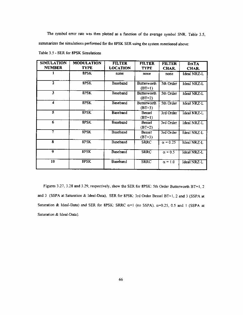
The symbol error rate was then plotted as a function of the average symbol SNR. Table 3.5,
summarizes the simulations performed for the 8PSK SER using the system mentioned above:
Table 3.5 - SER for 8PSK Simulations
SIMULATION MODULATION
NUMBER TYPE
1 8PSK
FILTER
LOCATION
none
FILTER
TYPE
none
FILTER
CHAR.
none
DATA
CHAR.
Ideal NRZ-L
2 8PSK Baseband Butterworth 5th Order Ideal NRZ-L
(BT=I)
3 8PSK Baseband Butterworth 5th Order Ideal NRZ-L
(BT=2)
4 8PSK Baseband Butterworth 5th Order Ideal NRZ-L
(aT=3)5 8PSK Baseband Bessel 3rd Order Ideal NRZ-L
(BT=I)
6 8PSK Baseband 3rd Order Ideal NRZ-LBessel
(BT=2)Baseband 3rd Order8PSK Bessel
(BT=3)
Ideal NRZ-L
8 8PSK Baseband SRRC ct = 0.25 Ideal NRZ-L
9 8PSK Baseband SRRC c_ = 0.5 Ideal NRZ-L
10 8PSK Baseband SRRC ct = 1.0 Ideal NRZ-L
,,9Figures 3.27, 3.28 and ,._9, respectively, show the SER for 8PSK: 5th Order Butterworth BT=I, 2
and 3 (SSPA at Saturation & Ideal-Data), SER for 8PSK: 3rd Order Bessel BT=I, 2 and 3 (SSPA at
Saturation & Ideal-Data) and SER for 8PSK: SRRC ct=l (no SSPA), ct=0.25, 0.5 and 1 (SSPA at
Saturation & Ideal-Data).
66

10 0
Figure 3.28 - SER for 8PSK: 3rd Order Bessel BT=I, 2 and 3 (SSPA at Saturation & Ideal Data)
67
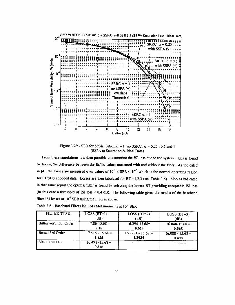
SER for 8PSK: SIRRCr=l (no SSPA); r=0.25,0.5,1 (SSPA Saturation Level, Ideal Data)10o
-;--+--"-:--_-"+" " ..... SRRC _=0.25 "---" ...... :..... "--" --_ - - with SSPA (x) : -"i i i i i
: " : : : ', : ', t10"+ ;=====.=====,=====_,=====+= ..........."::::::::::::::::::::::::::::" SRRC a=0.5
...... --_ ..... _ .... .+-'"_'I_" :--: t.- - - _ - - -- q ..... ,-'.... .,'..... ',..... +- with SSPA (*)
* i i i
: : : : : , ,,-a- '- .... -' ..... '--===+===--'- .... [ .... J
-_-_;.. , -._-_+_-":....." .... _'..... -' .... +- SRRC ct = I ----
+.+______.________++__+_-_______,,+ +.oss,.A.,,,I0"+ i_---" + ._ P.- -+',+ overlaps '==++:==.....
................... Theoretical -_ ............, .... I .... . ..... , .... .'," -, ," ",..... ...... _ .... -;..... i..... '
__- .... - .... - ..... ',..... ; , ,' ' ' : : i : : i :_ =i:. - = : I. J t. .t ........ t. .... j .......
_.,_ ..+__..] ; .', :i:::::__+_i_ms_s_P+_(,?>m" : : i i i i i i i +
-2 0 2 4 6 8 10 12 1,4 16 113Es/No (dB)
Figure 3.29 - SER for 8PSK: SRRC ct = 1 (no SSPA), ct = 0.25,0.5 and 1(SSPA at Saturation & Ideal Data)
From these simulations it is then possible to determine the [SI loss due to the system. This is found
by taking the difference between the Es/No values measured with and without the filter. As indicated
in [4], the losses are measured over values of I0 -3 _<SER _< l0 "2 which is the normal operating region
for CCSDS encoded data. Losses are then tabulated for BT = 1,2,3 (see Table 3.6). Also as indicated
in that same report the optimal filter is found by selecting the lowest BT providing acceptable ISI loss
(in this case a threshold of ISI loss < 0.4 dB). The following table gives the results of the baseband
filter ISI losses at 10"3SER using the Figures above:
Table 3.6 - Baseband Filters ISI Loss Measurements at 10"3SER
FILTER TYPE
Butterworth 5th Order
LOSS (BT=I)(dB)
17.86-15.68=2.18
LOSS (BT=2)
(dB)
16.294-15.68=
0.614
LOSS (BT=3)
(dB)
16.048-15.68 =
0.368
Bessel 3rd Order 17.515- 15.68 = 16.9734- 15.68 = 16.088- 15.68 =
1.835 1.2934 0.408
SRRC (ct=l.0) 16.498 -15.68 .......................0.818
68
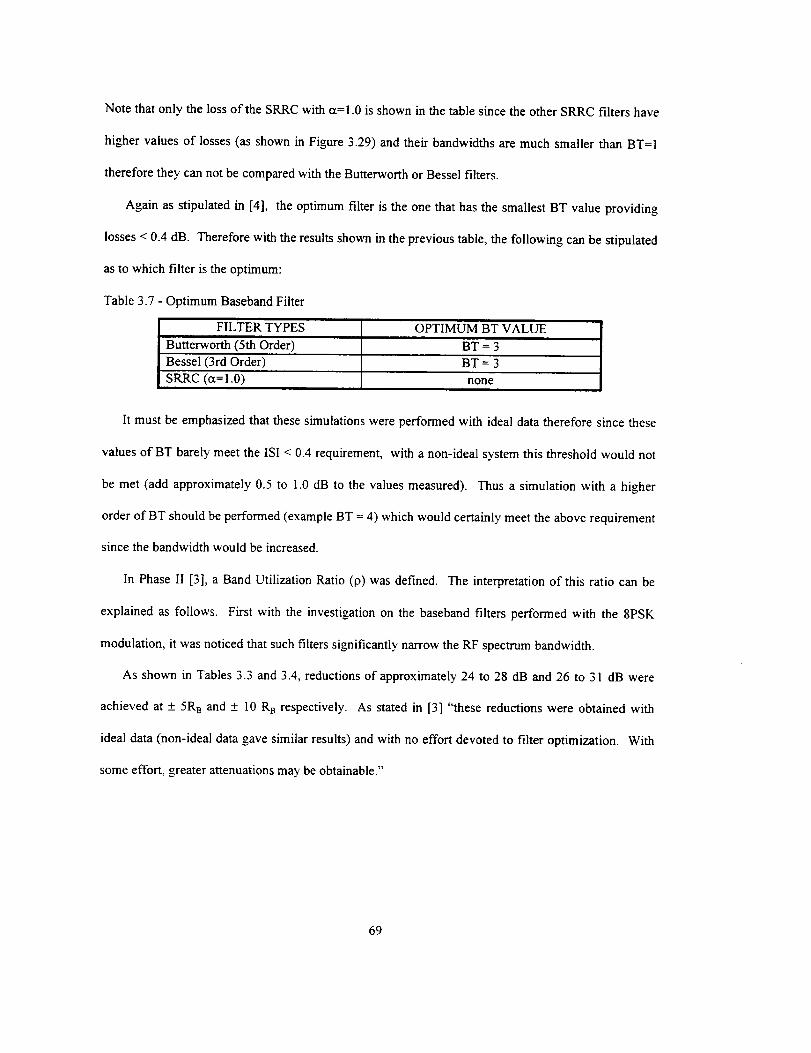
NotethatonlythelossoftheSRRCwitha=1.0isshowninthetablesincetheotherSRRCfiltershave
highervaluesof losses(asshowninFigure3.29)andtheirbandwidthsaremuchsmallerthanBT=I
thereforetheycannotbecomparedwiththeButterworthorBesselfilters.
Againasstipulatedin [4], theoptimumfilteristheonethathasthesmallestBTvalueproviding
losses<0.4dB. Thereforewiththeresultsshownintheprevioustable,thefollowingcanbestipulated
astowhichfilteristheoptimum:
Table3.7- OptimumBasebandFilter
FILTERTYPESButterworth(5thOrder)Bessel(3rdOrder) BT= 3SRRC(ct=1.0) none
OPTIMUM BT VALUE
BT= 3
It must be emphasized that these simulations were performed with ideal data therefore since these
values of BT barely meet the ISI < 0.4 requirement, with a non-ideal system this threshold would not
be met (add approximately 0.5 to 1.0 dB to the values measured). Thus a simulation with a higher
order of BT should be performed (example BT = 4) which would certainly meet the above requirement
since the bandwidth would be increased.
In Phase II [3], a Band Utilization Ratio (P) was defined. The interpretation of this ratio can be
explained as follows. First with the investigation on the baseband filters performed with the 8PSK
modulation, it was noticed that such filters significantly narrow the RF spectrum bandwidth.
As shown in Tables 3.3 and 3.4, reductions of approximately 24 to 28 dB and 26 to 31 dB were
achieved at + 5R B and + 10 RB respectively. As stated in [3] "these reductions were obtained with
ideal data (non-ideal data gave similar results) and with no effort devoted to filter optimization. With
some effort, greater attenuations may be obtainable."
69
Fromthis,twoquestionswereraised in Phase II about the significant change in the RF spectrum:
(1) - Can the number of spacecraft using a specific frequency band be increased if
baseband filtering is used ?; and
(2) - If the number of spacecraft using a specific frequency band can be increased, how
many more can be accommodated than wouM be the case if no filtering is used?
To answer to these questions, a frequency band Utilization Ratio (p) can be defined as :
p = Number of Spacecraft with Filtering Accommodated in Frequency Band
Number of Spacecraft without Filtering Accommodated in Frequency Band
An important assumption in deriving this ratio was made: the "spectra from spacecraft in adjacent
channels will be permitted to overlap one another provided that, at the frequency where the overlap
occurs, the signals are at least 50 dB below that of the main telemetry lobe (lst data sideband)." [3].
Using SPW, measurements were made using unfiltered and non-ideal data (the 2rid harmonic filter
was removed) to determine the frequency at which the data spectrum was 50 dB below the main lobe.
The Power Spectrum plots shown earlier were used to determine this 50 dB level. For example, for
ideal data without a spectrum shaping filter the -50riB point is situated at approximately 35 R B (refer
to Figure 3.2d) and using the Butterworth Filter (BT=I) with Ideal Data, the -50 dB point is
approximately at 2.5 RB (refer to Figure 3.4c), then the Utilization ratio, p, is equal to
p= 35RB =14.ZSRB
Note that the way the ratio is calculated in this example is different from the formula given previously
but the result is the same. The number of spacecraft with filtering accommodated in the frequency
band will be larger than if it was not filtered.
7O
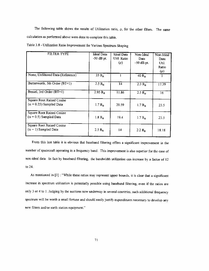
The following table shows the results of Utilization ratio, 19, for the other filters.
calculation as performed above were done to complete this table.
Table 3.8 - Utilization Ratio Improvement for Various Spectrum Shaping
FILTER TYPE
None, Unfiltered Data (Reference)
Butterworth, 5th Order (BT=I)
Bessel, 3rd Order (BT = 1)
Square Root Raised Cosine
(_ = 0.25) Sampled Data
Square Root Raised Cosine
(c_ = 0.5) Sampled Data
Square Root Raised Cosine
(_ = 1) Sampled Data
Ideal Data
-50 dB pt.
35 R B
2.5 R 8
2.95 R B
1.7 RB
1.8 R B
2.5 RB
Ideal Data
Util. Ratio
(p)
14
I 1.86
20.59
19.4
14
Non-Ideal
Data
-50 dB pt.
40 RB
2.3 RB
2.5 R B
1.7 RB
1.7 RB
2.2 RB
The same
Non-IdealData
Util.
Ratio
(o)
17.39
16
23.5
23.5
18.18
From this last table it is obvious that baseband filtering offers a significant improvement in the
number of spacecraft operating in a frequency band. This improvement is also superior for the case of
non-ideal data. In fact by baseband filtering, the bandwidth utilization can increase by a factor of 12
to 24.
As mentioned in [3] : "While these ratios may represent upper bounds, it is clear that a significant
increase in spectrum utilization is potentially possible using baseband filtering, even if the ratios are
only 3 or 4 to 1. Judging by the auctions now underway in several countries, such additional frequency
spectrum will be worth a small fortune and should easily justify expenditures necessary to develop any
new filters and/or earth station equipment."
71
Finally to complement this section on SER, it can be mentioned that different techniques can be
used to mitigate the effects due to the nonlinear bandlimited signal distortion present in these high data
rate satellites and therefore improve the End-to-End System Performance (SER). [1 I] presents a
development of the low-pass Volterra discrete-time model for a nonlinear communication channel.
More specifically, the dissertation in [11] is a study of adaptive Volterra equalizers on a downlink-
limited nonlinear bandlimited satellite channel. It is found that a receiver consisting of a fractionally-
spaced equalizer (FSE) followed by a Volterra equalizer (FSE-Volterra) gives improvement beyond
that gained by the Volterra equalizer. " Significant probability of error performance improvement is
found for multilevel modulation schemes. Also, it is found that probability of error improvement is
more significant for modulation schemes, constant amplitude and multilevel, which require higher
signal to noise ratios (i.e., higher modulation orders) for reliable operation". Furthermore, as
discussed in [ 12], in systems that have a strict power limitation and high data rate demands (example:
small satellite transmitting through NASA's TDRSS network), the dominant noise is present in the
uplink rather than the downlink channel. Therefore [12] shows that by modifying the standard
receiver for several digital modulation formats and through proper specification of receiver decision
regions, pulse shape and receiver filters, significant gains in performance can be produced. On the
other hand with respect to the bandwidth utilization, [ 13] introduces a way to develop technology and
equipment that would allow users to maximize their data throughput in an RF spectrum. All these
experiments where conducted in the Center for Space Telemetering and Telecommunications Systems
at New Mexico State University.
72
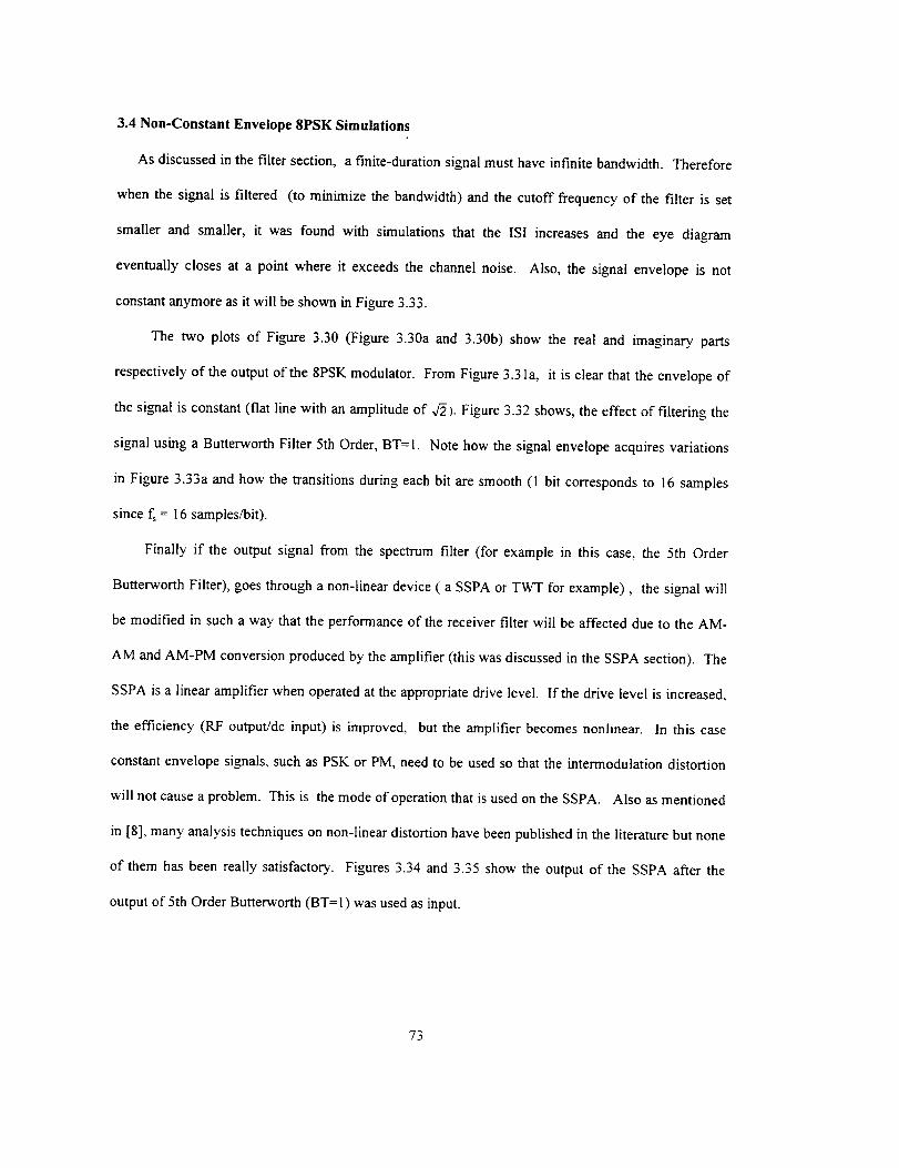
3.4 Non-Constant Envelope 8PSK Simulations
As discussed in the filter section, a finite-duration signal must have infinite bandwidth. Therefore
when the signal is filtered (to minimize the bandwidth) and the cutoff frequency of the filter is set
smaller and smaller, it was found with simulations that the ISI increases and the eye diagram
eventually closes at a point where it exceeds the channel noise. Also, the signal envelope is not
constant anymore as it will be shown in Figure 3.33.
The two plots of Figure 3.30 (Figure 3.30a and 3.30b) show the real and imaginary parts
respectively of the output of the 8PSK modulator. From Figure 3.3 la, it is clear that the envelope of
the signal is constant (flat line with an amplitude of 4-2). Figure 3.32 shows, the effect of filtering the
signal using a Butterworth Filter 5th Order, BT=I. Note how the signal envelope acquires variations
in Figure 3.33a and how the transitions during each bit are smooth (1 bit corresponds to 16 samples
since fs = 16 samples/bit).
Finally if the output signal from the spectrum filter (for example in this case, the 5th Order
Butterworth Filter), goes through a non-linear device ( a SSPA or TWT for example), the signal will
be modified in such a way that the performance of the receiver filter will be affected due to the AM-
AM and AM-PM conversion produced by the amplifier (this was discussed in the SSPA section). The
SSPA is a linear amplifier when operated at the appropriate drive level. If the drive level is increased,
the efficiency (RF output/dc input) is improved, but the amplifier becomes nonlinear. In this case
constant envelope signals, such as PSK or PM, need to be used so that the intermodulation distortion
will not cause a problem. This is the mode of operation that is used on the SSPA. Also as mentioned
in [8], many analysis techniques on non-linear distortion have been published in the literature but none
of them has been really satisfactory. Figures 3.34 and 3.35 show the output of the SSPA after the
output of 5th Order Butterworth (BT=I)was used as input.
73

Thus when PSK (non-filtered and constant envelope) goes through a high powered amplifier (in the
non-linear or linear region), the same waveform at the input will be reproduced at the output due to
the constant envelope of the data. This can be seen in Figures 3.36 and 3.37, where no spectrum
shaping filter was used thus the signal going through the SSPA has a constant envelope.
74
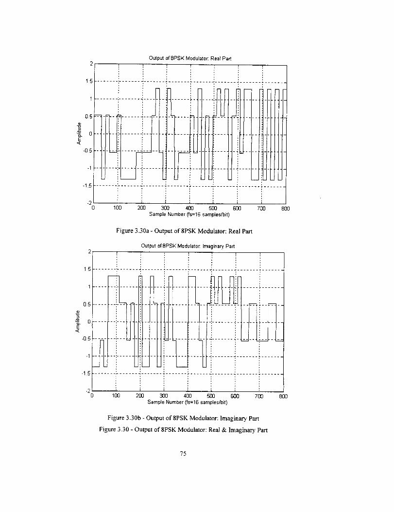
E,<
1.5
1
0.5
0
-0.5
-1
Output of BPSK Modulator: Real Part
700 800
ii iiiiiiiii ilii................ li--
-1.5........ " ...... " ....... "....... " ...............
-2 I i , ,0 100 200 300 400 500 600
Sample Number (fs=16 samples/bit)
Figure 3.30a - Output of 8PSK Modulator: Real Part
Output of SPSK Modulator: Imaginary Part2
1.5 ........................................ :.......................
.... ' ....... ; ........... 4 ...... _-.......
0.5 ' -
_ iiiiiiiiiii} o
_ iill-05
_1 iiiii__ iii......-1.5
-2 r I I I I
0 100 200 300 400 500 600 700 800Sample Number (fs=16 samples/bit)
Figure 3.3Ob - Output of 8PSK Modulator: Imaginary Part
Figure 3.30 - Output of 8PSK Modulator: Real & Imaginary Part
75
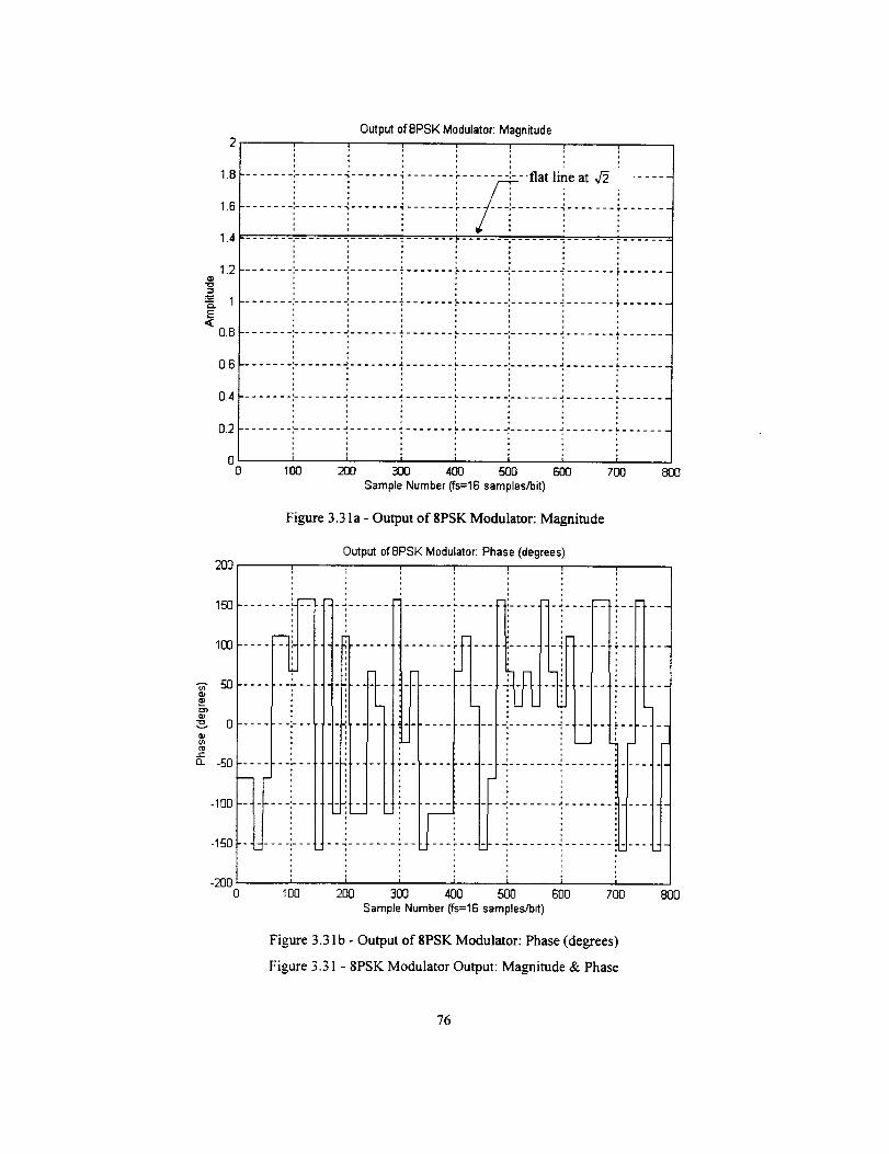
Output of BPSK Modulator; Magnitude2 = = =
: ,.1.8 ................ _ ....... . ....... r ....... :-- fiat line at J'2 ......
/-7,,=
i............... ,....... r---/---!--..... _..............1.6
1.4
1.2 ........ ........ _..............................................
E,<
08
05
0.4
0.2
00
........ , ....... .J ....... .L ....... I. ....... , ....... j ....... & .......
I I I I I
100 200 300 400 500 600 700 800
Sample Number (fs=16 samples/bit)
Figure 3.3 la - Output of 8PSK Modulator: Magnitude
2O0
150
100
_- 5O,m==
0
05
o_ -50
-100
-150
-2OO0
Output of BPSK Modulator: Phase (degrees)i i i i = =
i i "iiiiii i1....................
............. r_
.°.
.-. J
: ',i l , i i
100 200 300 400 500 BOO 700 BOO
Sample Number (fs=16 samples/bit)
Figure 3.31 b - Output of 8PSK Modulator: Phase (degrees)
Figure 3.31 - 8PSK Modulator Output: Magnitude & Phase
76
Output of 5th Order Butterworth Filter (BT=I): Real Part
1.5
0.5
'-- 0E
<
-0.5
-1
-1.5
-20
1.5
iiiiiiiiiiiiiii!iiii-i!iiiiiiii-il.........
I I I I | I
I00 200 300 400 500 600 700 800
Sample Number (fs=16 samples/bit)
Figure 3.32a - Output of 5th Order Butterworth Filter (BT=I): Real Part
05
__ 0E
,<
-0.5
-1
-1.5
-20
Output of Sth Order lutterworth Filter (13T=1): Imaginary Part
I-; ....... J ....... ÷.....
,,
1O0 200 300 400 500 600 700 800
Sample Number (fs=16 samples/bit)
Figure 3.32b - Output of 5th Order Butterworth Filter (BT=I): Imaginary Part
Figure 3.32 - 5th Order Butterworth Filter (BT=I) Output: Real & Imaginar3: Part
77
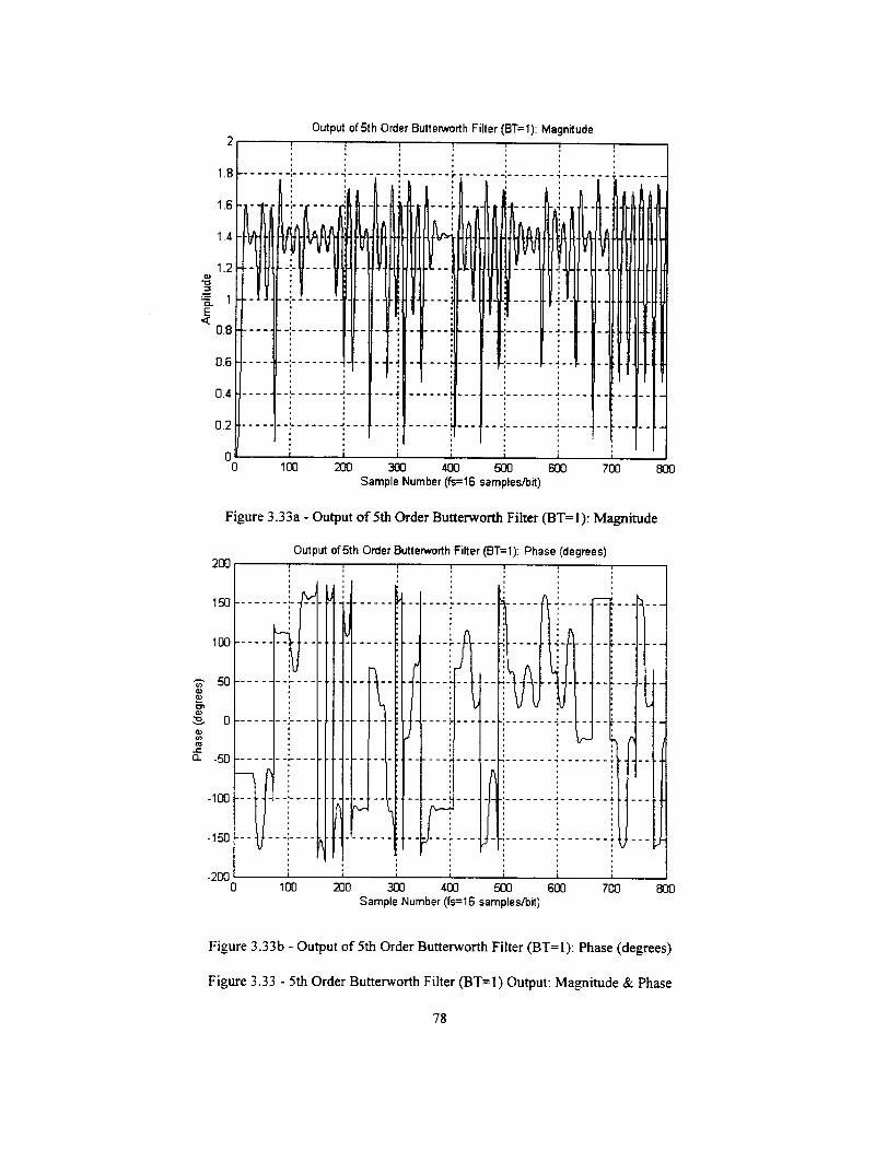
E,<
Output of Sth Order Butterworth Filler (BT=I): Magnitude
2 I ¢ 1 i ,
,18.6..........iii iiii ijl_'._:_.-....._--__."....iiii[_-i.....iiiil--_i--ii-i_.'•......1.4
1.2
1 i ,-. _j0.8 ,--
[1.4 .......
0.2 .--
0 0 100 200 300 400 _ E;O(] 700 B00
Sample Number (fs=16 samples/bit)
Figure 3.33a - Output of 5th Order Butterworth Filter (BT=I): Magnitude
200.
150
lO0
100 200 300 400 ,500 600 700 B00
Sample Number (fs=16 samples/bit)
Figure 3.33b - Output of 5th Order Butterworth Filter (BT=I)'. Phase (degrees)
Figure 3.33 - 5th Order Butterworth Filter (BT=I) Output: Magnitude & Phase
78
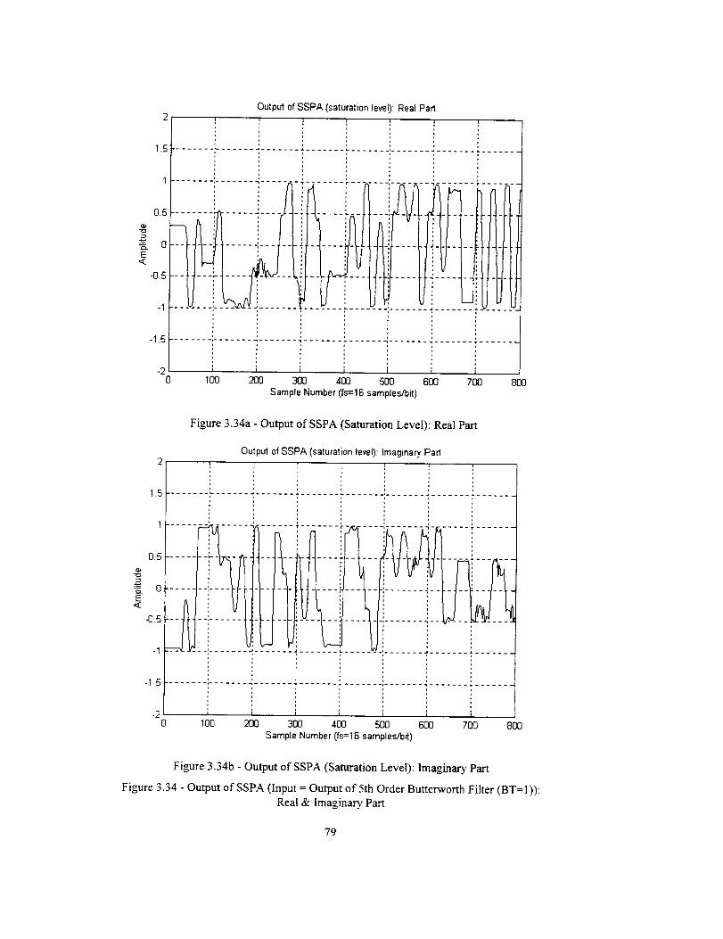
Output of SSPA (saturation level):Real Part
1.5 ....... :....... -1....... ; ....... ,_....... i....... ",'....... ! ......
i......._......._......._.......__ ___ _ iI : : : : !...................
05 ...... i ..... " ...... " ..... " -- .....
o ...... . ..... -_...... _ .... i "i .....
<-o5.1 _ li__....... " - -' _i ....
-. .... i.... .j........ '
l:ii:i:i:i....:i ___
L-
-1.5
-2 = i I t i100 200 300 400 500 600 700 800
Sample Number (fs=16 samples/bit)
Figure 3.34a - Output of SSPA (Saturation Level): Real Part
Output of SSPA (saturation level): Imaginary Pad2 i '
i1.5 ................................................................
1 .....
......Ii ii o_o ..........!__
-0.5 ..........
-I ............ i................. i
,,-2 ' i l
0 1O0 200 300 400 500 600 700 800Sample Number (fs=16 samples/bit)
Figure 3.34b - Output of SSPA (Saturation Level): Imaginary Part
Figure 3.34 - Output of SSPA (Input = Output of 5th Order Butterworth Filter (BT=l)):
Real & Imaginary Part
?9
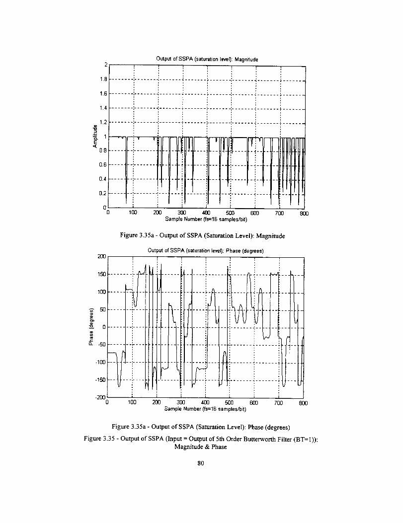
Output of SSPA (saturation level): Magnitude2 i i z i
I 8 ........ ,....... ._ ..................• r -1
1.6 ........ ,....... _............... , ....... ,........................
1.4 ...................................................... _ .......
1.2 ...................................................... . .......
E,<
0.8
0.6
0.4
0.2
00
• v
iiliiii i
I I
100 200
..L .... i
I I
3OO 4117
- lf IIYi"-- -t-,'1" ..... J,.....
__.!....... i .....
5(13 6OO
Sample Number (fs=16 samples/bit)
I
7O0
Figure 3.35a - Output of SSPA (Saturation Level): Magnitude
Output of SSPA (saturation level): Phase (degrees)200 ......
i : :150- -
100
a_ -50 .
-100
-150
I
.......___J._L................ r --i
-200 ' '0 100 200
,J i
3O0 4OO
l iiiiiiiiiiiiiiiililli i =
500 600 700
Sample Number (fs=16 samples/bit)8OO
Figure 3.35a - Output of SSPA (Saturation Level): Phase (degrees)
Figure 3.35 - Output of SSPA (Input = Output of 5th Order Butterworth Filter (BT= I)):
Magnitude & Phase
8O
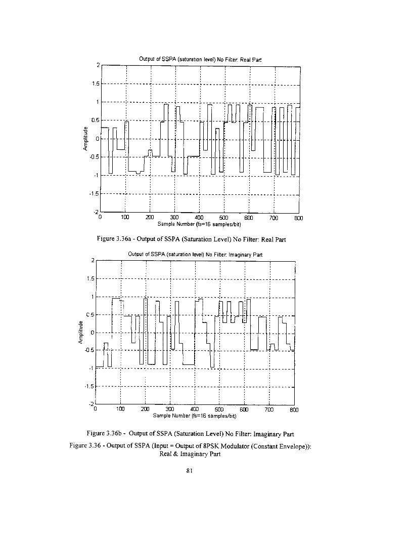
0.5
-- 0E
<
-0.5
-I
1.5
.............................. ¢.
Output of SSPA (saturation level) No Filter: Real PartI i
T
"15 1 .............. " ............... i ............................. t
-2 '0 100 200 300 400 500 600 700 800
Sample Number (fs=16 samples/bit)
Figure 3.36a - Output of SSPA (Saturation Level) No Filter: Real Part
Output of SSPA (saturation level) No Filter: Imaginary Part
E<
0.5
0
-05 ---i .........
.... ' ....... _,h- ..... T......H
-210 100 200 300 400 500 600 700 800
Sample Number (fs=16 samples/bit)
Figure 3.36b - Output of SSPA (Saturation Level) No Filter: Imaginary Part
Figure 3.36 - Output of SSPA (Input = Output of 8PSK Modulator (Constant Envelope)):
Real & Imaginary. Part
81
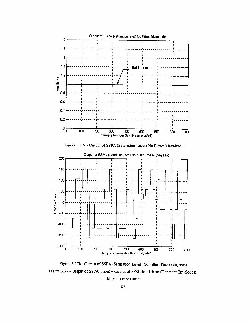
1.2
z=. 1E<
0.8
Output of 8SPA saturation level) No Filter. Magnitude2 =
1.8 ........ ,....... _ ....... • ....... _....... :....... _ ....... , .......
1.6 ............... = ....... • ............... :....... _ ........ - ......
1.4 ................................. fiat line at I ..................
.......................... S ..............................
........ =....... .._ ....... J. ....... L. ....... , ....... .J ....... J. .......
0.6 ................................................................
0.4 ........................................................ " .......
0.2 ................................................................
!0 i i , i l i i
0 1130 200 300 400 500 600 700 800
Sample Number (fs=16 samples/bit)
Figure 3.37a- Output of SSPA (Saturation Level)No Filter: Magnitude
CO
(D
03
£
tO
200
150
100
50
0
.,50 ---
7-1130 --.
-150 -- -
-2000
I
.._ ._"_"_"_"_"_'_:. _ _
...... %.-
.--,---
.__,.--
.--_--
I
100
Output of SSPA (saturation level) No Filter: Phase (degrees)i
: -iiiiiiiiii i!i-- iiiii !ii
= J ] 1 1
200 3OO 400 500 6OO 700
Sample Number (fs=16 samples/bit)
8OO
Figure 3.37b - Output of SSPA (Saturation Level) No Filter: Phase (degrees)
Figure 3.37 - Output of SSPA (Input = Output of 8PSK Modulator (Constant Envelope)):
Magnitude & Phase
82
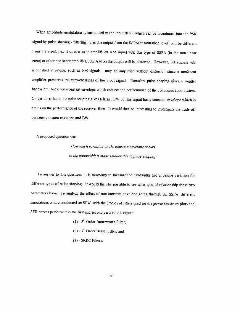
When amplitude modulation is introduced in the input data ( which can be introduced into the PSK
signal by pulse shaping - filtering), then the output from the SSPA(at saturation level) will be different
from the input, i.e., if ones tries to amplify an AM signal with this type of SSPA (in the non-linear
zone) or other nonlinear amplifiers, the AM on the output will be distorted. However, RF signals with
a constant envelope, such as FM signals, may be amplified without distortion since a nonlinear
amplifier preserves the zero-crossings of the input signal. Therefore pulse shaping gives a smaller
bandwidth but a non-constant envelope which reduces the performance of the communication system.
On the other hand, no pulse shaping gives a larger BW but the signal has a constant envelope which is
a plus on the performance of the receiver filter. It would then be interesting to investigate the trade-off
between constant envelope and BW.
A proposed question was:
How much variation in the constant envelope occurs
as the bandwidth is made smaller due to pulse shaping?
To answer to this question, it is necessary to measure the bandwidth and envelope variation for
different vypes of pulse shaping. It would then be possible to see what type of relationship these two
parameters have. To analyze the effect of non-constant envelope going through the SSPA, different
simulations where conducted on SPW with the 3 types of filters used for the power spectrum plots and
SER curves performed: in the first and second parts of this report:
(1) - 5 th Order Butterworth Filter;
(2) - 3 rd Order Bessel Filter; and
(3) - SRRC Filters.
83
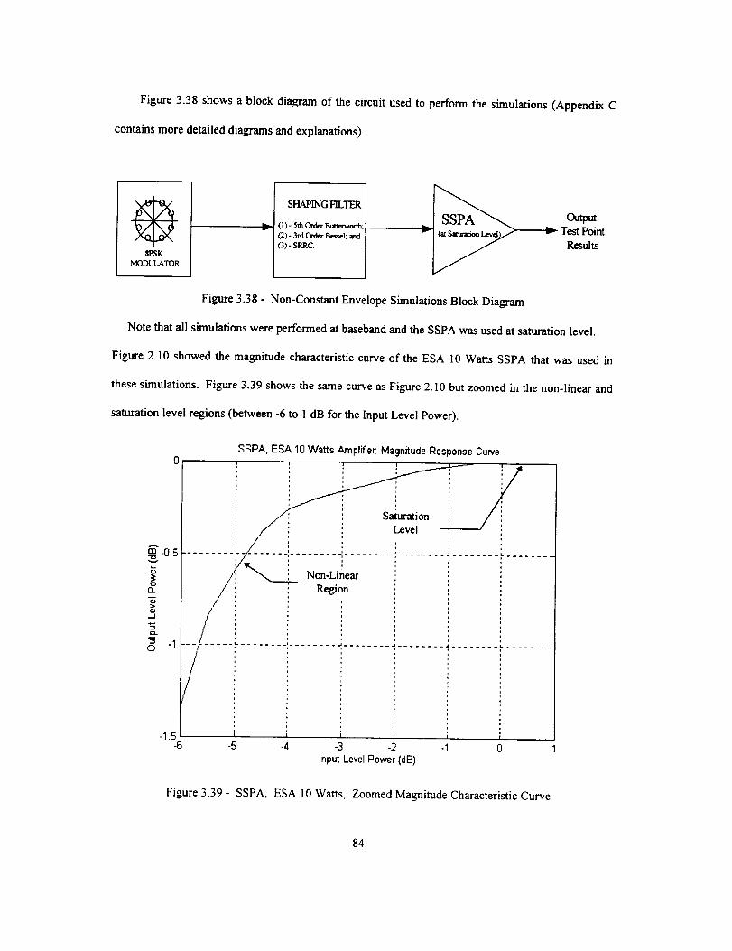
Figure3.38showsablockdiagram oft_he circuit used to perform the simulations (Appendix C
contains more detailed diagrams and explanations).
SPSK
MODULATOR
SHAPINGFILTER
_- (t)- 5thOrd=-Sm't_ortlx(2)- 3rdOrd_B_._I;(3)- SP.RC.
m_v
Figure 3.38 - Non-Constant Envelope Simulations Block Diagram
Note that all simulations were performed at baseband and the SSPA was used at saturation level.
Figure 2.10 showed the magnitude characteristic curve of the ESA 10 Watts SSPA that was used in
these simulations. Figure 3.39 shows the same curve as Figure 2.10 but zoomed in the non-linear and
saturation level regions (between -6 to 1 dB for the Input Level Power).
o
._J
o._
= -1o
SSPA, ESA 10 Watts Amplifier: MagnitudeResponse Curve
_ : ', ,Saturation i /Level
.................i.... ................................' : Region
?/',
__.t. ........ , ........ J ........ .J ........ .i ....... t. ........
-1.5 =-6 -5 -4 -3 -2 -1 0
Input Level Power (dB)
Figure 3.39 - SSPA, ESA 10 Watts, Zoomed Magnitude Characteristic Curve
84
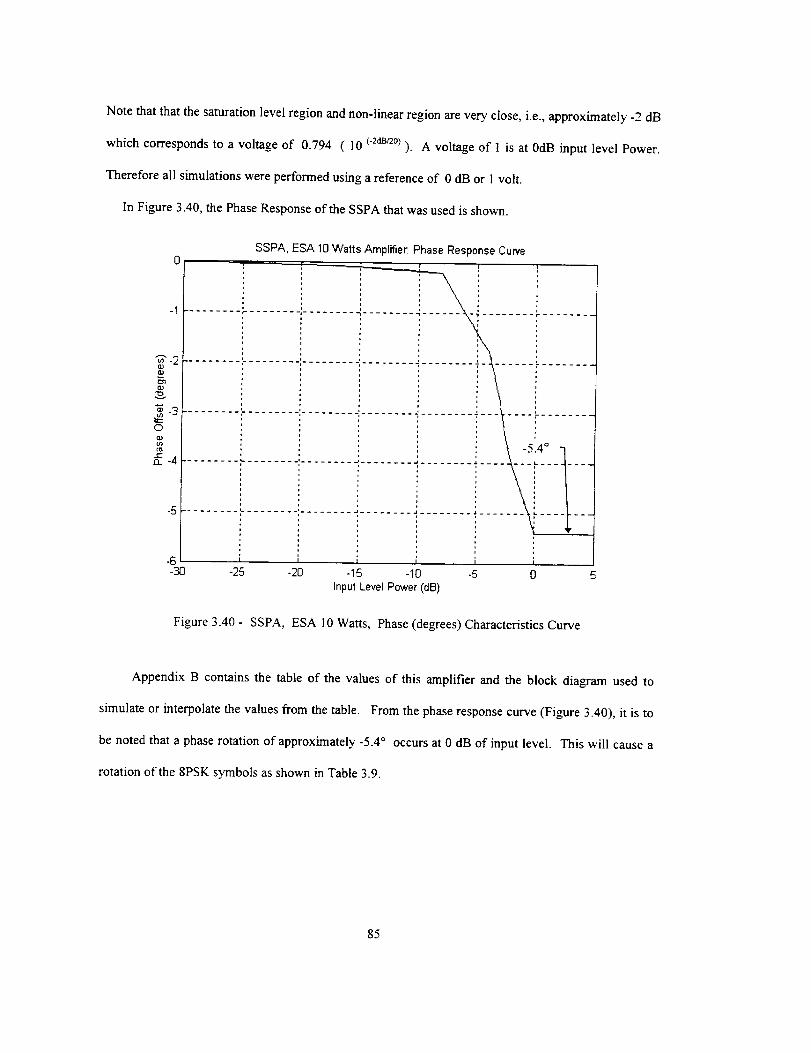
Notethatthatthesaturationlevelregionandnon-linearregionareveryclose,i.e.,approximately-2dB
whichcorrespondstoavoltageof 0.794( 10¢-2_czo)). A voltage of 1 is at 0dB input level Power.
Therefore all simulations were performed using a reference of 0 dB or 1 volt.
In Figure 3.40, the Phase Response of the SSPA that was used is shown.
-1
_-2lit)
"$-3
(9
e.-12_-4
-5
SSPA, ESA 10Watts Amplifier: Phase Response Curve
.................. ........ -_........ 4 ....... _ ................
..................................... _
....... ?1...................................................
1
-6 i i i I i i-30 -25 -20 -15 -10 -5 0 5
Input LevelPower (dB)
Figure 3.40 - SSPA, ESA 10 Watts, Phase (degrees) Characteristics Curve
Appendix B contains the table of the values of this amplifier and the block diagram used to
simulate or interpolate the values from the table. From the phase response curve (Figure 3.40), it is to
be noted that a phase rotation of approximately -5.4 ° occurs at 0 dB of input level. This will cause a
rotation of the 8PSK symbols as shown in Table 3.9.
85
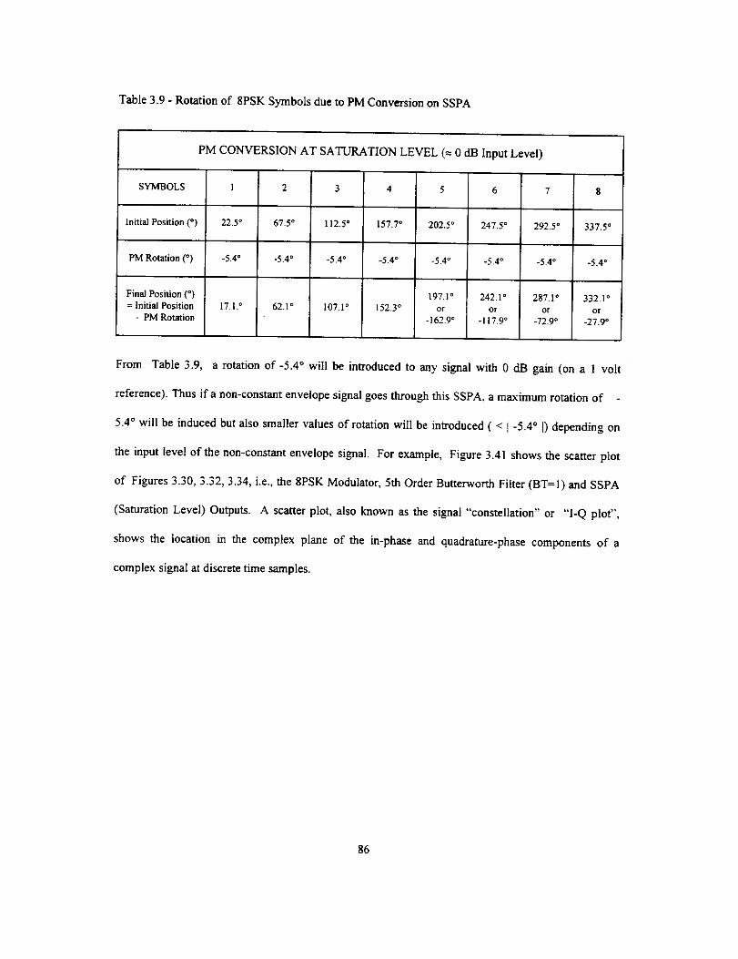
Table 3.9 - Rotation of 8PSK Symbols due to PM Conversion on SSPA
PM CONVERSION AT SATURATION LEVEL (_ 0 dB Input Level)
SYMBOLS I 2 3 4 5 6 7 g
Initial Position (*) 22.5* 67.5 ° 112.5" 157.7" 202.5 ° 247.5 ° 292.5* 337.5 °
PM Rotation (*) -5.4 ° -5.4 ° -5.4* -5.4* -5.4 ° -5.4 ° -5.4 ° -5.4 °
Final Position( °) 197.1 ° 242.1" 287.1 ° 332.1 °= Initial Position 17.1 .° 62.1 ° 107.1 * 152.3 ° or or or or
- PM Rotation -162.9 ° -117.9 ° -72.9 ° -27.9 °
From Table 3.9, a rotation of-5.4 ° will be introduced to any signal with 0 dB gain (on a 1 volt
reference). Thus if a non-constant envelope signal goes through this SSPA, a maximum rotation of -
5.4 ° will be induced but also smaller values of rotation will be inlroduced ( < I -5 .40 ]) depending on
the input level of the non-constant envelope signal. For example, Figure 3.41 shows the scatter plot
of Figures 3.30, 3.32, 3.34, i.e., the 8PSK Modulator, 5th Order Butterworth Filter (BT=I) and SSPA
(Saturation Level) Outputs. A scatter plot, also known as the signal "constellation" or "I-Q plot",
shows the location in the complex plane of the in-phase and quadrature-phase components of a
complex signal at discrete time samples.
86
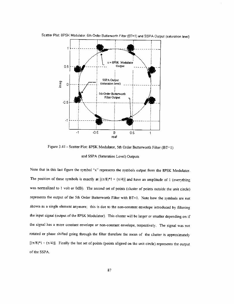
Scatter Plot: 8PSK Modulator, 5th Order Butterworth Filter (BT=I) and SSPA Output (saturation level)
__ x = gPSK Modulator
Output
,,
SSPA Output
(saturation level)
,,5th Order Butterworth
,. Filter Output
\ :\ :
I I I
-0.5 0 0.5real
Figure 3.41 - Scatter Plot: 8PSK Modulator, 5th Order Butterworth Filter (BT= 1)
and SSPA (Saturation Level) Outputs
Note that in this last figure the symbol "x" represents the symbols output from the 8PSK Modulator.
The position of these symbols is exactly at [(_t/8)*l + (n/4)] and have an amplitude of I (everything
was normalized to 1 volt or 0dB). The second set of points (cluster of points outside the unit circle)
represents the output of the 5th Order Butterworth Filter with BT=I. Note how the symbols are not
shown as a single element anymore; this is due to the non-constant envelope introduced by filtering
the input signal (output of the 8PSK Modulator). This cluster will be larger or smaller depending on if
the signal has a more constant envelope or non-constant envelope, respectively. The signal was not
rotated or phase shifted going through the filter therefore the mean of the cluster is approximately
[(n/8)*i + (rd4)]. Finally the last set of points (points aligned on the unit circle) represents the output
of the SSPA.
87
Note that this time the symbols have been rotated (_ -5.4 °) due to the AM/PM conversion
introduced by the SSPA. Also the symbols are aligned on the unit circle since the SSPA is operating at
saturation level (0 dB or l volt).
To be able to create this scatter plot from Figures 3.30, 5.32 and 3.34, the following procedure was
followed. First a simulation on SPW was performed using the block diagram shown in Figure 3.34 (a
more detailed diagram in shown and explained in Appendix C). Then when the simulation was
completed, the American Information Code for Information Interchange (ASCII) file containing the
complex values of the output of the SSPA for example (signal shown in Figure 3.30) was transferred
(File Transfer Protocol (FTP)) to a Personal Computer (PC 486 66 MHz) where the signal was
sampled to its optimum value to produce the SSPA Output scatter plot shown in Figure 3.41. For
example, for the signal in Figure 3.30, a signal delay equal to 20 samples had to be used to get the
optimum scatter plot. This delay of 20 samples was calculated as follows:
First the pulse shaping filter (5th Order Butterworth Filter (BT= l)) and SSPA introduced a delay of
12 samples (includes the delay due to the transition) and since the sampling of the received bit has to
occur in the middle of the bit ( fs/2 where fs = sampling frequency = #samples/bit), then
T _._plt,gme = (Delay of 5th Order Butterworth filter (BT=I) and SSPA) + (f J2)
where for the 5th Order Butterworth Filter (BT=I), the sampling frequency = f_= 16
samples/bit (for more information on the choice of the value of f, refer to Appendix C).
Thus
T s_pI_g_me = 12 samples + (16 samples/bit/2) = 12 + 8
T _vli_g _me = 20 samples
88
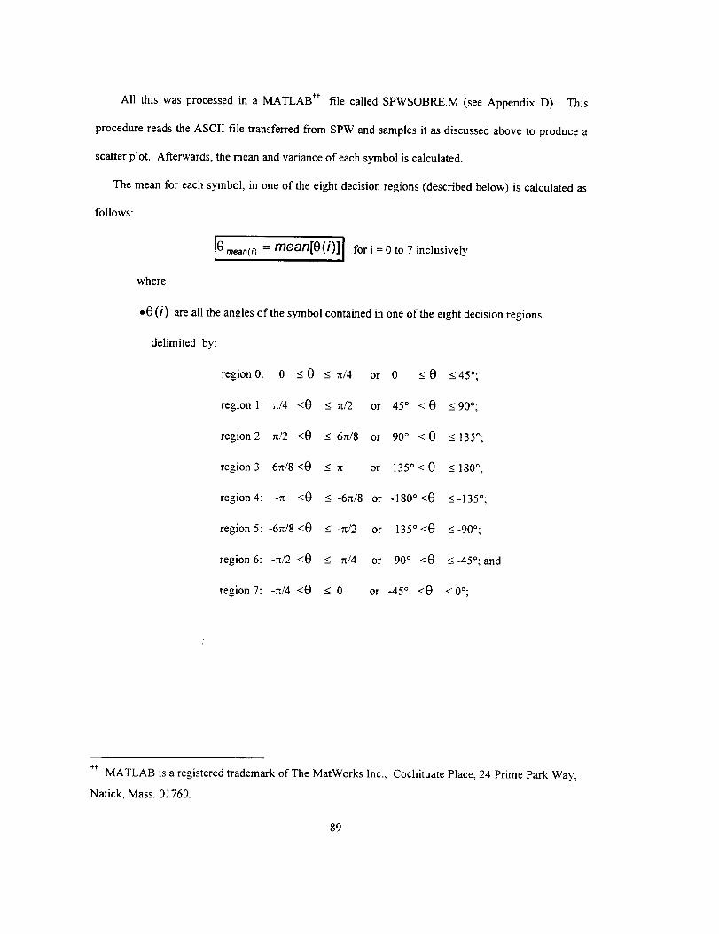
All thiswasprocessedin a MATLABt* file calledSPWSOBRE.M(seeAppendixD). This
procedurereadstheASCIIfiletransferredfromSPWandsamplesit asdiscussedabovetoproducea
scatterplot.Afterwards,themeanandvarianceofeachsymboliscalculated.
The mean for each symbol, in one of the eight decision regions (described below) is calculated as
follows:
IO mean(i) = mean[O(i)][ fori=0to 7 inclusively
where
• 0 (i) are all the angles of the symbol contained in one of the eight decision regions
delimited by:
region 0: 0 < 0
region I: n/4 <0
region2:zt/2 <0
region 3:6n/8 <0
region4: -rt <0
reglon 5:-6n/8 <0
region 6:-zt/2 <0
reg,on 7:-n/4 <0
< _/4 or 0 <0 _<45°;
_< rt/2 or 45 ° < 0 _<90°;
_< 6n/8 or 90 ° <0 _<135°;
< rt or 135 °<0 _<180°;
_< -6zff8 or -180 ° <0 _<-135°;
<_ -rt/2 or -135 ° <0 _<-90°;
_< -n/4 or -90 ° <0 -<-45°;and
_< 0 or -45 ° <0 < 0%
,t MATLAB is a registered trademark of The MatWorks Inc., Cochituate Place, 24 Prime Park Way,
Natick, Mass. 01760.
89
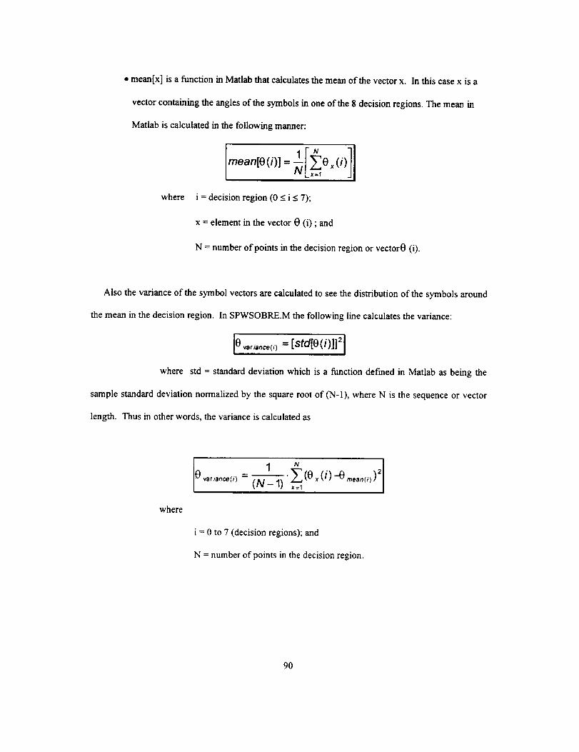
• mean[x]isafunctioninMatlabthatcalculatesthemeanofthevectorx. In this case x is a
vector containing the angles of the symbols in one of the 8 decision regions. The mean in
Matlab is calculated in the following manner:
where i = decision region (0 < i < 7);
x = element in the vector 0 (i) ; and
N = number of points in the decision region or vector0 (i).
Also the variance of the symbol vectors are calculated to see the distribution of the symbols around
the mean in the decision region. In SPWSOBRE.M the following line calculates the variance:
]0 = [std[O(i)]]21
where std = standard deviation which is a function def'med in Matlab as being the
sample standard deviation normalized by the square root of (N-l), where N is the sequence or vector
length. Thus in other words, the variance is calculated as
where
1 N IO_""=c'l (N-1)'_"(Ox(i)-O"*""('l)2_=,
i = 0 to 7 (decision regions); and
N = number of points in the decision region.
90
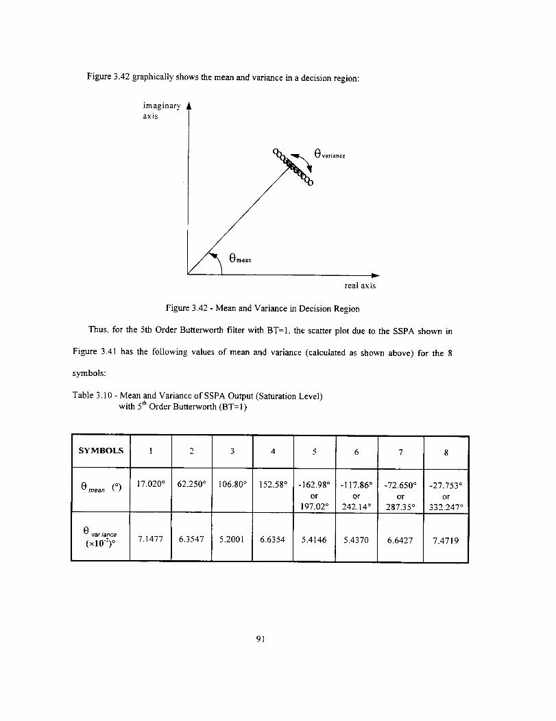
Figure3.42graphicallyshowsthemeanandvarianceinadecisionregion:
imaginaryaxis
Ovariane¢
v
real axis
Figure 3.42 - Mean and Variance in Decision Region
Thus, for the 5th Order Butterworth filter with BT=I, the scatter plot due to the SSPA shown in
Figure 3.41 has the following values of mean and variance (calculated as shown above) for the 8
symbols:
Table 3.10 - Mean and Variance of SSPA Output (Saturation Level)with 5 thOrder Butterworth (BT= 1)
SYMBOLS
0,,e_ (o)
O var iance
(xl0-:) °
17.020 °
7.1477
62.250 °
6.3547
106.80 °
5.2001
4
152.58 °
6.6354
-162.98 °
or
197.02 °
5.4146
-117.86 °
or
242.14 °
5.4370
-72.650 °
or
287.35 °
6.6427
-27.753 °
or
332.247 °
7.4719
91
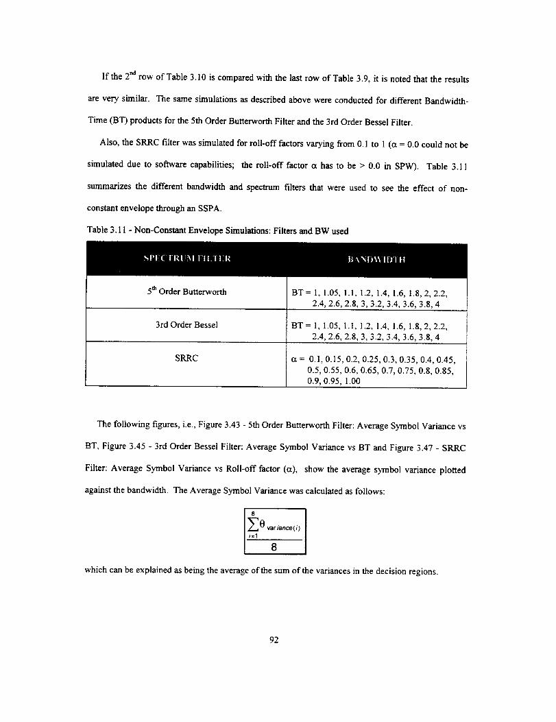
If the2"drowof Table 3.10 is compared with the last row of Table 3.9, it is noted that the results
are very similar. The same simulations as described above were conducted for different Bandwidth-
Time (BT) products for the 5th Order Butterworth Filter and the 3rd Order Bessel Filter.
Also, the SRRC filter was simulated for roll-off factors varying from 0.1 to 1 (ct = 0.0 could not be
simulated due to software capabilities; the roll-off factor a has to be > 0.0 in SPW). Table 3.11
summarizes the different bandwidth and spectrum filters that were used to see the effect of non-
constant envelope through an SSPA.
Table 3.11 - Non-Constant Envelope Simulations: Filters and BW used
5th Order Butterworth
3rd Order Bessel
SRRC cx = 0.1, 0.15, 0.2, 0.25, 0.3, 0.35, 0.4, 0.45,
0.5, 0.55, 0.6, 0.65, 0.7, 0.75, 0.8, 0.85,0.9, 0.95, 1.00
The following figures, i.e., Figure 3.43 - 5th Order Butterworth Filter: Average Symbol Variance vs
BT, Figure 3.45 - 3rd Order Bessel Filter: Average Symbol Variance vs BT and Figure 3.47 - SRRC
Filter: Average Symbol Variance vs Roll-off factor (a), show the average symbol variance plotted
against the bandwidth. The Average Symbol Variance was calculated as follows:
_ 0 variance(i)
i=1 -'8
which can be explained as being the average of the sum of the variances in the decision regions.
92
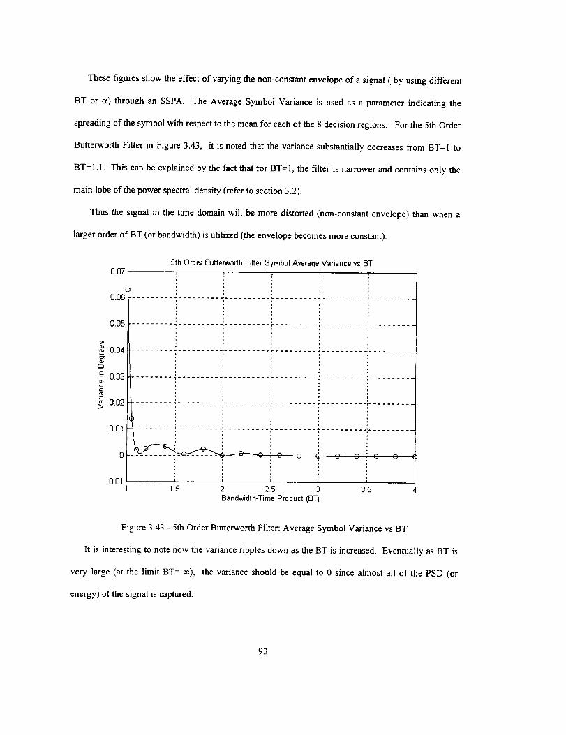
Thesefiguresshowtheeffectofvaryingthenon-constantenvelopeof asignal( byusingdifferent
BTor t_) through an SSPA. The Average Symbol Variance is used as a parameter indicating the
spreading of the symbol with respect to the mean for each of the 8 decision regions. For the 5th Order
Butterworth Filter in Figure 3.43, it is noted that the variance substantially decreases from BT=I to
BT=1.1. This can be explained by the fact that for BT=I, the filter is narrower and contains on]y the
main lobe of the power spectral density (refer to section 3.2).
Thus the signal in the time domain will be more distorted (non-constant envelope) than when a
larger order of BT (or bandwidth) is utilized (the envelope becomes more constant).
0.05
p 0.04
rn
.E 0.03
C
0.o2
0.01
0
o0.01
5th Order Butterworth Filter Symbol Average Variance vs BT
I
I
,,
........ J ........ , .......... L ......... .I .......... , ..........
I--_ r _I _ _ _ __ _ 0 ' 0 _ _
I
1.5 2 2.5 3 3.5 4Bandwidth-Time Product (137-)
Figure 3.43 - 5th Order Butterworth Filter: Average Symbol Variance vs BT
It is interesting to note how the variance ripples down as the BT is increased. Eventually as BT is
very large (at the limit BT = oo), the variance should be equal to 0 since almost all of the PSD (or
energy) of the signal is captured.
93
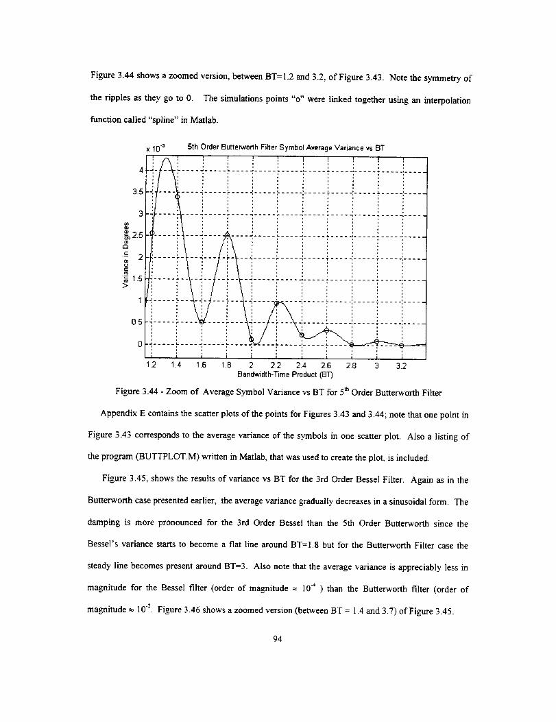
Figure 3.44 shows a zoomed version, between BT= 1.2 and 3.2, of Figure 3.43. Note the symmetry of
the ripples as they go to 0. The simulations points "o" were linked together using an interpolation
function called "spline" in Matlab.
35
0 : .... :--- ;-
I i i i , i i1.2 1.4 1.6 1.8 2 2.2 2.4 2.6 2.8 3 3.2
Bandwidth-Time Product (BT)
Figure 3.44 - Zoom of Average Symbol Variance vs BT for 5 th Order Butterwotth Filter
Appendix E contains the scatter plots of the points for Figures 3.43 and 3.44; note that one point in
Figure 3.43 corresponds to the average variance of the symbols in one scatter plot. Also a listing of
the program (BUTTPLOT.M) written in Matlab, that was used to create the plot, is included.
Figure 3.45, shows the results of variance vs BT for the 3rd Order Bessel Filter. Again as in the
Butterworth case presented earlier, the average variance gradually decreases in a sinusoidal form. The
damping is more pronounced for the 3rd Order Bessel than the 5th Order Butterworth since the
Bessel's variance starts to become a fiat line around BT=I.8 but for the Butterworth Filter case the
steady line becomes present around BT=3. Also note that the average variance is appreciab]y less in
magnitude for the Bessel filter (order of magnitude _ 10 -4 ) than the Butterworth filter (order of
magnitude = 10 2. Figure 3.46 shows a zoomed version (between BT = 1.4 and 3.7) of Figure 3.45.
94
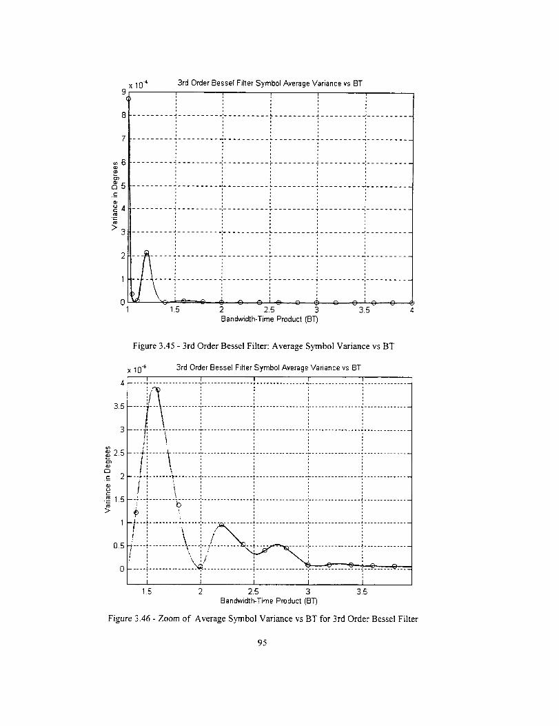
O0
_D_D
C3
t-
(15
>
x 10.4 3rd Order Bessel Filter Symbol Average Variance vs BT9 , J I I I
: ,, ', ,, ;......... J ......... ' .......... L ......... a. .......... *__
7 .......... ' ........ " ......... ' ......... " ......... ' ........
; ',6 .......... " .......... :........................................
' ,
4 ........ _ .................... _ .................... :.........
........ .J .......... , .......... L,. ......... _, .......... , .........
,, : : ,,
'1__i'_....................--- i:,,::---iiiiiiiiiiiiiiiiiiiiiiiiiiill_ _ ..............15 2 25 3 35
Bandwdth-Time Producl (13"1-)
Figure 3.45 - 3rd Order Bessel Filter: Average Symbol Variance vs BT
x 10 .6 3rd Order Bessel Filter Symbol Average Variance vs BT
3°..../__.............................................................................
_ _.,............ _..........................................................................b
1 -}---; ......... L...... :................ ; ................ :................ _..............
o5{ ....;..........\ ...._.._.i._._....._.......... _................_..............
I I I I I15 2 25 3 3.5
Bandwidth-Time Product (BT)
2.5
.E 2
C
,---1.5>
Figure 5.46 - Zoom of Average Symbol Variance vs BT for 3rd Order Bessel Filter
95
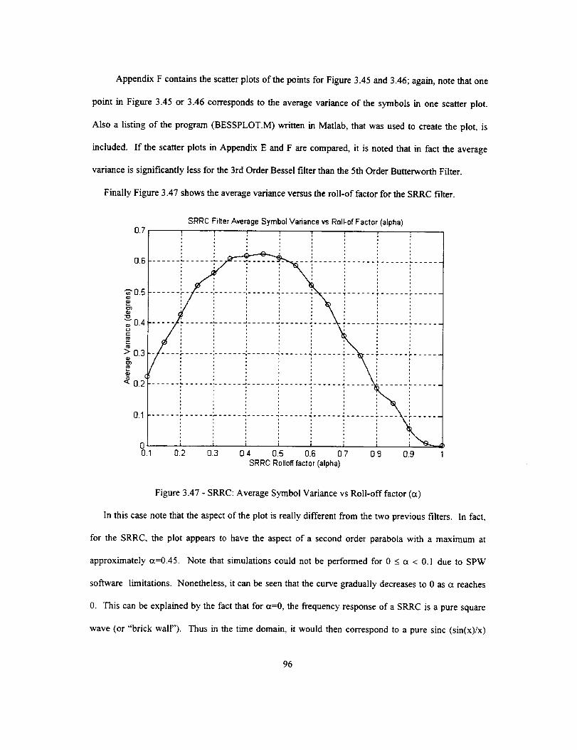
Appendix F contains the scatter plots of the points for Figure 3.45 and 3.46; again, note that one
point in Figure 3.45 or 3.46 corresponds to the average variance of the symbols in one scatter plot.
Also a listing of the program (BESSPLOT.M) written in Matlab, that was used to create the plot, is
included. If the scatter plots in Appendix E and F are compared, it is noted that in fact the average
variance is significantly less for the 3rd Order Bessel filter than the 5th Order Butterworth Filter.
Finally Figure 3.47 shows the average variance versus the roll-of factor for the SRRC filter.
SRRC Filter Average Symbol Variance _s Roll-of Factor (alpha)I I
0.6 .......... :-
I I ;
i
r ..... , ....... i......l
T ...... r ......
i
i i0.2 0.3 0.4 0.5 06 0.7
SRRC Roltoff factor (alpha)
00.1 0.8 0.9 1
Figure 3.47 - SRRC: Average Symbol Variance vs Roll-off factor (a)
In this case note that the aspect of the plot is really different from the two previous filters. In fact,
for the SRRC, the plot appears to have the aspect of a second order parabola with a maximum at
approximately _x=0.45. Note that simulations could not be performed for 0 _<ct < 0. I due to SPW
software limitations. Nonetheless, it can be seen that the curve gradually decreases to 0 as cc reaches
0. This can be explained by the fact that for ct=0, the frequency response of a SRRC is a pure square
wave (or "brick wall"). Thus in the time domain, it would then correspond to a pure sinc (sin(x)/x)
96
functionwhichwouldhavethe zero crossings at the sampling frequency therefore eliminating any ISI.
For the case where ct reaches 1, the average variance also decreases toward 0 (but it does not reach
it). This can be explained since the SRRC filter has a bigger BW for higher ct therefore allowing
more of the power spectrum to be included in the transmission; this is the same result as increasing the
BT for the Butterworth or Bessel Filter. Finally note how the magnitude of the average variance is
larger for the SRRC filter than the Butterworth and Bessel.
Appendix G contains the scatter plots of the points for Figure 3.47. Also a listing of the program
(SRRCPLOT.M) written in Matlab, that was used to create the plot, is included. If the scatter plots in
Appendix E, F and G are compared, it is noted that in fact the average variance is significantly bigger
for the SRRC filter than the 3rd Order Bessel filter or the 5th Order Butterworth Filter.
97
Chapter 4
CONCLUSIONS AND RECOMMENDATIONS
From the simulations on 8PSK Baseband Filtering performed in the Center for Space Telemetering
and Telecommunications Systems at NMSU, the following conclusions can be made on the PSD, SER
and Non-Constant Envelope:
With respect to PSD and SER for the 8PSK signal which is an extension of the work performed during
Phase I, II and III (refer to [1], [2], [3] and [4]) of this study :
• In-band spurious emissions are more present and more evident for the Bessel Filter than the
Butterworth Filter (BT=I). With respect to the sideband attenuation, it was found that the values
of attenuation for the 3rd Order Bessel are comparable to the 5th Order Butterworth (refer to
Tables 3.3 and 3.4 in the report).
For SRRC filters with a = 0.25 and cx = 0.5, the bandwidth is narrower than the Butterworth and
Bessel Filters but the attenuation is less at high frequencies. Nonetheless, the absence of spurious
emissions is a net advantage. For SRRC ¢t = 1, the bandwidth is wider than the two previous
SRRC filters and the absence of in-band spurious emissions was again noticed. Less sideband
attenuation was recorded for this roll-offfactor compared with t_ = 0.25 and a = 0.5.
For SElL it was found that the Butterworth and Bessel Filters just barely meet the threshold of ISI
loss < 0.4 dB at SER = 10 .3 . Also the SRRC filters do not meet this specification. Since this
threshold is barely met by the first two filters and this simulation was performed with only ideal
data and system it seems reasonable that a simulation with BT = 4 should be performed which
would certainly meet the threshold.
98
Fromtheseresults,it canbestipulatedthatthe5th OrderButterworthhasa smalladvantage
comparedto theotherfilters. Alsomoresimulationsshouldbeperformedon thepowerspectrum
contentdependingonthevalueof BTthatmeetsthethresholdmentionedabove.Therefore,for
exampleforBT= 4 , thepowerspectrumplotsshouldbeproducedto beableto calculatethenew
BandUtilizationratio,19.
Overall,it wasshownbyusingbasebandfilteringthebandwidthutilizationcanbeimprovedbya
factorof approximately12to 24withBT=I and8PSK(seeTable3.8 in thisreport)whichcan
significantlyincreasethespectrumutilization.InPhaseII (referto [3]),it wasdemonstratedthatfor
BPSK,thisbandwidthutilizationcanbepotentiallyincreasedfrom6to 10timeswithBT=I. Thus
withrespecttobandwidth,8PSKgivesbetterresults(usingthesamebitrate).
Toincreaseourknowledgewithrespecttoanon-linearsatellitechannel,specificmeasurementswere
performedontheNon-ConstantEnvelopeof thesignalsgoingthroughthenon-linearSSPA.These
simulationshavenotbeenpreviouslyreported.
Thetradeoffsbetweenconstantenvelopeandbandwidthwereobserved with simulations for the
5th Order Butterworlh Filter, 3rd Order Bessel Filter and SRRC Filter. The more shaped the pulse
(to decrease the bandwidth), the more non-constant the envelope of the signal becomes therefore
increasing errors due to non-linearities in the system.
It was found that the amplitude of the Average Symbol Variance of the signal
using the 3rd Order Bessel is much less than for the 5th Order Butterworth
Filter. Also the amplitude for the 3rd Order Bessel Filter damps toward zero
around BT=I.8 where for the 5th Order Butterworth Filter this damping will
occur around BT=3. These curves have the aspect of a sinusoidal function
decreasing exponentially toward zero; and
99
TheAverageSymbolVariancevs_ for theSRRCwasfoundto be quite
different than the two previous specmun shaping filters. This plot looks more
like a second order parabola with a maximum at approximately ct = 0.45. Also
the amplitude is significantly larger than the two previous filters.
Suggestions for further _tudy
• A non-ideal system can be used for future simulations for SER. This non-ideal system should be
predetermined with respect to what kind of components have to be used and the amount of error
they introduce.
• Increase the BT to 4 and perform more simulations for PSD and SER.
• For the non-constant envelope simulations more simulations should be performed using different
orders of filters for Butterworth and Bessel:
From these simulations it might be possible to find a general expression on how
the variance of the symbols is altered by changing BT. This expression should
have the following form: a*exp(-x)*sin(x) for the Butterworth and Bessel
Filters; and
It would then be possible to predict, with a general equation, when the BT has
no real effect on the shaping of a pulse.
100
REFERENCES
[i] Warren L. Martin and Tien M. Nguyen, "CCSDC - SFCG Efficient Modulation Methods Study,
A Comparison of Modulation Schemes, Phase I: Bandwidth Utilization (Response to SFCG
Action Item 12/32)," SFCG-13, Ottawa Canada, 13-21 October 1993, report dated 24 September
1993.
[2] Dr. Manfred Otter, "CCSDC - SFCG Efficient Modulation Methods Study, A Comparison of
Modulation schemes, Phase lb: A Comparison of QPSK, OQPSK, BPSK, and GMSK
Modulation Systems (Response to SFCG Action Item 12/32)," European Space Agency/ESOC,
Member CCSDS Subpanel 1E, (RF and Modulation), June 1994.
[3] Warren L. Martin and Tien M. Nguyen, "CCSDC - SFCG Efficient Modulation Methods Study,
A Comparison of Modulation Schemes, Phase 2: Spectrum Shaping (Response to SFCG Action
Item 12/32)," SFCG Meeting, Rothenberg, Germany 14-23 September 1 994, report dated
August 1994.
[4] Warren L. Martin, Tien M. Nguyen, Aseel Anabtawi, Sami M. Hinedi, Loc V. Lam and Mazen
M. Shihabi, "CCSDC - SFCG Efficient Modulation Methods Study Phase 3: End-to-End System
Performance," Jet Propulsion Laboratory', May 1995.
[51 Israel Korn, "The Effect of Pulse Shaping and Transmitter Filter on the Performance of FSK-
DPD and CPM-DPD in Satellite Mobile Channel," IEEE Journal on Selected Areas in
Communications, Vol.13, NO. 2, February 1995.
[61 G. Benelli, V. Capellini, E. Del Re and R. Fantacci, "Evaluation of Constant-Envelope Signals
Degradation due to Band-Limited Filtering," IEEE International Conference on Communications
'86, Toronto (Ontario) Canada, 1986.
[7] G. Bharatula, J. Sekfy and J. Millot, " Simulation Studies for Digital Satellite Communications,"
20th International Electronics Convention & Exhibition, Melbourne, Australia, October 1985.
101
[8] Leon W. Couch II, "Digital and Analog Communication Systems," Macmillan Publishing
Company, 1993, Fourth Edition.
[9] Stephen Horan, "Introduction to PCM Telemetering Systems," CRC Press Inc. 1993.
[10] Lonnie C. Ludeman, "Fundamentals of Digital Signal Processing," John Wiley & Sons, 1986.
[ 11 ] Alberto Gutierrez, Jr., "Equalization and Detection for Digital Communication over Non-Linear
Bandlimited Satellite Communication Channels," PhD Dissertation by, New Mexico State
University, December 1995.
[12] Theodore John Wolcott, "Uplink-Noise Limited Satellite Communication Systems," Ph.D.
Dissertation, New Mexico State University, December 1995.
[13] Michael Ross, William Osborne and Gregory .lean-Baptiste, " Bandwidth Utilization LDRD,
Report for Phase I, Simulation of 32 QAM TCM in SPW," Center for Telemelry Research,
Klipsch School of Electrical Engineering, New Mexico State University.
[14] "SPW - The DSP Framework Communications Library Reference", by Comdisco Systems,
Product Number: SPW8015, March 1994.
[ 15] "Signal Processing WorkSystem DSP Library Reference", by Alta Group of Cadence Design
Systems, Inc. Product Number: SPWS015, March 1995.
102
APPENDIX A
SPW DETAIL DIAGRAMS
FOR
PSD AND SER SIMULATIONS
This appendix contains the detailed diagrams of the overall system used for the PSD and the SER
simulations. Explanations on how these simulations were performed will be given.
A.I PSD Detailed Diagram
Figure A. 1 shows a detailed block diagram of the system used to simulate the PSD with different
spectrum shaping filters. First, a MPSK Source block is used and since the simulations were
performed for 8PSK the corresponding parameters were given (see right top comer of Figure A. 1) to
have an 8 level output. The output of this block is saved in a library "rubensigs/modout" for later use.
For a more detailed aspect of this block refer to Figure 2.3 in the report. The output of this modulator
is then introduced in the "Baseband Spectrum Shaping Filter" (for this case the Butterworth Filter is
shown). Figure A.2 shows the contents of this Butterworth Filter Block. When performing
simulations the filter order was set to 5 for the Butterworth filter, the attenuation at the passband edge
was set to 3dB. These two parameters were kept the same for all the simulations. The sampling
frequency was set to 250 samples/bit to be able to have as much spectrum as possible giving a range
from -125 RB to 125 RB .
103
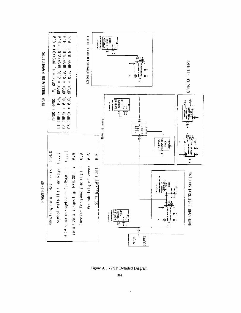
t_I,I
<Kr_
O-
t'_
_.J
'v
COG_
cvLI.
L_
rv"
II II II I_
II II II
,,dd_
_d_d
II II II
II
II II II
g
I
d
O
N
_ N
ZiZ
E -5C_. EE _
d d _ d
un Z -- -_
e--
_ 2P _ iL I
m w i
t'_ _ _m
N
Z
-,@
I
_"? i
__ Z
i e_
Figure A. 1 - PSD Detailed Diagram
104
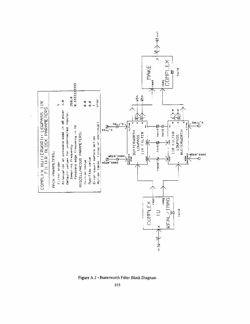
Figure A.2 - Butte_'onh Filter Block Diagram
105
Forthe"PassbandEdgeFrequency"parameter,B,thevaluewassetto 1/3sinceforthissimulation
theBT of the filter was 1 thus
BT = B* (Symbol Period) = B*(1/Symbol Rate) = B/R s
= B/(R B /k)= B*L/R B
where Rs = Symbol Rate (symbols/sec);
RB = Bit Rate = I bit/sec (set by default for these simulations);
k = log2 8 = 3; and
B = Passband Edge Frequency or Single-Sided 3dB Bandwidth.
Thus BT = B*(3/1) = 3B =1 which implies that the Passband Edge Frequency = B = I/3 as shown
in Figure A.2 and explained above. If the simulation had to be performed for BT=2, then the Passband
Edge Frequency, B, would be equal to 2/3 and for BT=3, B=I. The output of this filter is also saved in
a file for later use. The next block of Figure A. 1 is the SSPA which is explained in detail in Appendix
B. It is to be noted that the output of the SSPA is also saved in a file. Finally in the study of the PSD
of 8 PSK, a 2nd Harmonic Filter (4th Order Butterworth Filter) follows the power amplifier. This type
of filter is frequently used after the power amplifier to protect users of other bands. The parameters of
this filter can be set in the same manner as explained above for the 5th Order Butterworth. Also for
this filter, the output is sent into a file.
In the case where non-ideal data had to be simulated in the system the parameter "zeta" or data
asymmetry in the top left comer box in Figure A.1 had to be set in following manner. First the
parameter" Symbol Rate (Hz) or Rsym" was set to 1/3 (RB / _.) as explained above. Using this result,
the parameter "N (#samples/symbol = fJRsym)" is equal to
f, _ 250samples I sec
R,_ (113)symbol / see= 750samples / symbol
106
andtheparameter"zeta"isdefinedasN*0.02since,asexplainedin thisreport,CCSDSlimitsdata
asymmetry(orzetainourcase)to_+2%(ratioof timedurationof a 1totimedurationofa0).Thus
using the formula and result for N shown above:
Nx0.02 = 750x0.02 = 15 samples/symbol of data asymmetry.
This number would then be entered next to the zeta parameter. Also another parameter that has to
be changed when simulating with non-ideal data are the "Probability of Zero" or data imbalance which
was defined in this report as the probability of a bit ! versus the probability of a bit 0. CCSDS limits
data imbalance to 0.45. Thus this value of 0.45 would then be entered for the "Probability of Zero".
The "Carrier Frequency Wc (Hz)" parameter was set to 0 for all the simulations since these were
performed at baseband. Also the "SSPA Backoff (dB)" parameter was set to 0 since the simulations
were performed at saturation level (except when the 10 dB Backoff simulations were performed; then
the value of SSPA Backoffwas set to I0 dB).
When these parameters are set, the simulation is started by using the "run" function in SPW. For
the PSD simulations, 300 000 samples were used. After the simulation is terminated, the FFT function
in SPW is used (FFT Points was set to 524288 for better accuracy as discussed in section 3.2 of this
report) to plot the PSD diagrams. The final diagrams of the PSD are shown in this report, section 3.2.
107
A.2 SER Detailed Diagram
The detailed diagram from SPW that was used to measure the SER and produce the corresponding
SER Curves is shown in Figure A.3. Basically this circuit takes the output signal of the matched filter
(since NRZ-L is the data format, a sliding integrator was used as the matched filter. For more
information about the matched filter refer to section 2.7 in this report) which is the signal that was
distorted through the channel and compares it with the input signal. This comparison is performed by
a delay & phase meter which tries to correlate the non-distorted signal with the distorted one. When
the best correlation is found, the distorted and non-distorted PSK signals are converted to their
corresponding symbol numbers. Afterwards these symbol numbers are compared in a "Simple Error
Rate Estimator" to fred the Symbol Error Rate (SER).
All this is performed in real time and is shown on the screen of the Sparc-10 Sun Station as it can
be seen in the two boxes " Display and Control" and "Error Rate Display" in Figure A.3. Finally
Figure A.4 shows a detailed block diagram for the AWGN that was used in the SPW simulations.
108
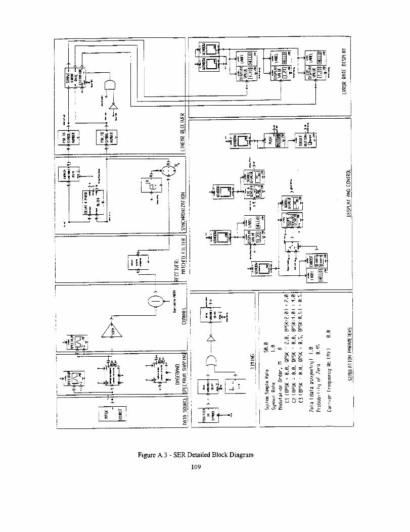
|
|
...z
I
i _ •Z
A,.
i I
÷
!.k
- _ t.r7 e_
° . °
§
i
z_
Figure A.3 - SER Detailed Block Diagram
109

Signal
AVERAGEx COMPLEX
POWER ,t/2
AveSigPwr COMPLEX (Es WHITE z /2
NOISE
Signal{/_'Nx _N I. COMPLEX I plus
_[_ -J/.,. / No t' (" o.,_ _ I"mag zl , Noise
value-80 _ I ''''''" _'_- "'"
v-J.e= :o " Es/N_(dB) .. L_x I; ] ES/NOF-b
Sample Rate = 8.0 _ '_ iSymbol Rate= 1.0 _ y X" z
v_ue= 100
• ............ . .......................... °°._
Figure A.4 - Detailed Block Diagram for the AWGN
110
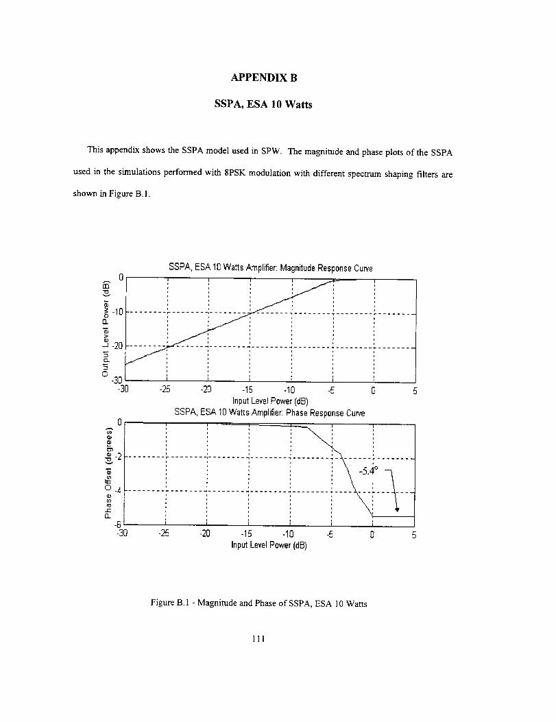
APPENDIX B
SSPA, ESA 10 Watts
This appendix shows the SSPA model used in SPW. The magnitude and phase plots of the SSPA
used in the simulations performed with 8PSK modulation with different spectrum shaping filters are
shown in Figure B.I.
[D
O
O.
>C0
c'_
£3
-10
-2O
-3O
SSPA, ESA 10 Watts Amplifier: Magnitude Response Curve
', I ,
' J ii t , J
-30 -25 -20 -15 -10 -_ 0
Input Level Power (dB)
SSPA, ESA 10 Watts Amplifier: Phase Response Curve' i I
i
-_-2 .............................................. - ..............
O -4 ......................................
m
e-
0-
-6 f i i-30 -25 -20 -15 -10 -5 0
Input Level Power (dB)
Figure B.I - Magnitude and Phase of SSPA, ESA 10 Watts
111
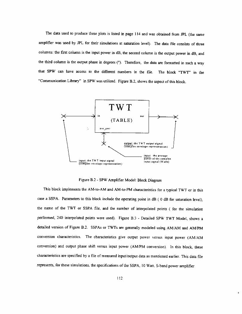
The data used to produce these plots is listed in page 114 and was obtained from JPL (the same
amplifier was used by JPL for their simulations at saturation level). The data file consists of three
columns: the first column is the input power in dB, the second column is the output power in dB, and
the third column is the output phase in degrees (o). Therefore, the data are formatted in such a way
that SPW can have access to the different numbers in the file. The block "TWT" in the
"Communication Library" in SPW was utilized. Figure B.2, shows the aspect of this block.
TWTX ) i. out ) )(
(TABLE)
L ave_pwr Ioutput: the TWT output signal
comp-Tex envelope representation)input: the average
power of the complexinput: the TWT input signal input signal (Watts)(complex envelope representation)
Figure B.2 - SPW Amplifier Model: Block Diagram
This block implements the AM-to-AM and AM-to-PM characteristics for a typical TWT or in this
case a SSPA. Parameters to this block include the operating point in dB ( 0 dB for saturation level),
the name of the TWT or SSPA file, and the number of interpolated points ( for the simulation
performed, 240 interpolated points were used). Figure B.3 - Detailed SPW TWT Model, shows a
detailed version of Figure B.2. SSPAs or TWTs are generally modeled using AM/AM and AM/PM
conversion characteristics. The characteristics give output power versus input power (AM/AM
conversion) and output phase shift versus input power (AM/PM conversion). In this block, these
characteristics are specified by a file of measured input/output data as mentioned earlier. This data file
represents, for these simulations, the specifications of the SSPA, 10 Watt, S-band power amplifier
112
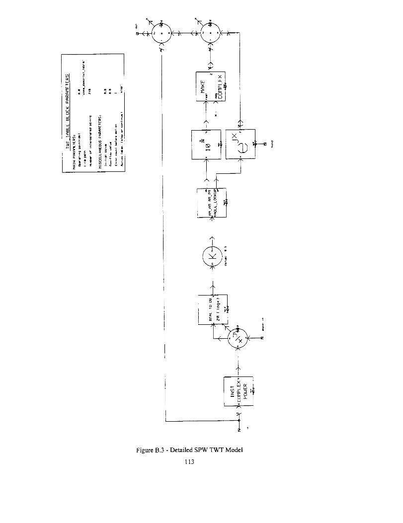
r_
_e
c ua
_ _ -__:
I T /,
:!If!R
C
h
" l
i:Figure B.3 - Detailed SPW TWT Model
113
used by the European Space Agency (ESA). As stipulated in [14]," the measured data in the data file,
consists of relative power levels, referenced to saturation point. That is, the input power data are the
input power relative to that which causes saturation at the output, and the output power data are the
output power relative to the power at saturation. This allows the characteristics to be modeled around
the point where an input envelope value of unity gives an output envelope value of unity. Thus, in the
measured data, 0 dB input power corresponds to 0 dB output power."
114
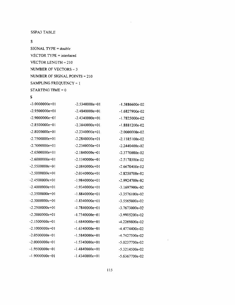
SSPA3TABLE
$
SIGNALTYPE=double
VECTORTYPE= interlacedVECTORLENGTH=210
NUMBEROFVECTORS= 3
NUMBEROFSIGNALPOINTS=210
SAMPLINGFREQUENCY= 1STARTINGTIME=0
$
-3.0000000e+01
-2.9500000e+01
-2.9000000e+01
-2.8500000e+01
-2.8000000e+01
-2.7500000e+01
-2.7000000e+01
-2.6500000e+01
-2.6000000e+01
-2.5500000e+01
-2.5000000e+01
-2.4500000e+01
-2.4000000e+01-2.3500000e+01
-2.3000000e+01
-2.2500000e+01
-2.2000000e+01
-2.1500000e+01
-2.1000000e+01
-2.0500000e+01
-2.0000000e+01
-1.9500000e÷01-1.9000000e+01
-2.5340000e+01
-2.4840000e+01
-2.4340000e+01
-2.3840000e+01
-2.3340000e+01
-2.2840000e+01
-2.2340000e+01-2.1840000e+01
-2.1340000e+01
-2.0840000e+01
-2.0340000e+01
-1.9840000e+01
-1.9340000e+01
-1.8840000e+01
-1.8340000e+01
-1.7840000e+01
-!.7340000e+01
-1.6840000e+01
-1.6340000e+01-1.5840000e+01
°1.5340000e+01
-1.4840000e+0!
-I.4340000e+01
-1.5886600e-02
-1.6827900e-02-1.7825000e-02
-1.8881200e-02
-2.0000000e-02
-2.1185100e-02
-2.2440400e-02
-2.3770000e-02
-2.5178500e-02
-2.6670400e-02
-2.8250700e-02
-2.9924700e-02
-3.1697900e-02-3.3576100e-02
-3.5565000e-02
-3.7673000e-02
-3.9905200e-02
-4.2269800e-02
-4.4774400e-02
-4.7427500e-02
-5.0237700e-02
-5.3214500e-02
-5.6367700e-02
115
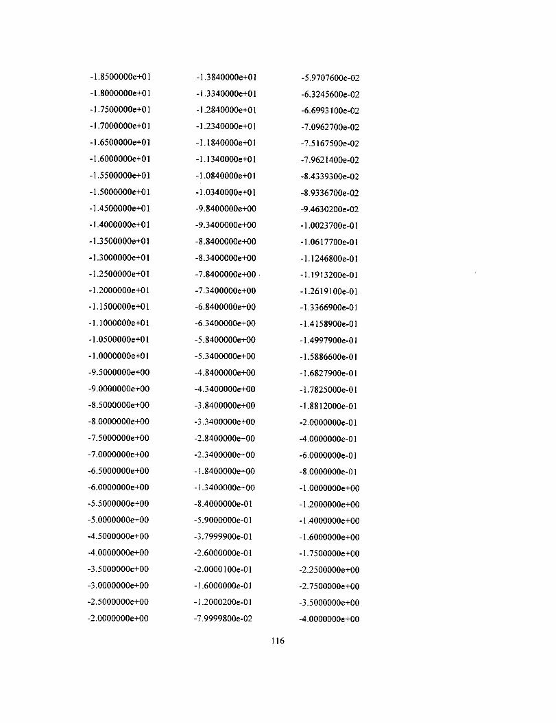
-1.8500000e+01
-l.8000000e+O1-1.7500000e+01
-l.7000000e+Ol
-1.6500000e+01
-1.6000000e+Ol
-1.5500000e+01
-l.5000000e+O1
-1.4500000e+01-l.4000000e+O1
-1.3500000e+01
-1.3000000e+Ol-1.2500000e+01
-1.2000000e+Ol
-1.1500000e+O1
-1.1000000e+O1
-1.0500000e+Ol
-1.O000000e+OI
-9.5000000e+00
-9.0000000e÷O0
-8.5000000e+00
-8.0000000e+O0
-7.5000000e+00
-7.0000000e+O0
-6.5000000e+00
-6.0000000e+O0
-5.5000000e+00
-5.0000000e+O0
-4.5000000e+00
-4.0000000e+O0
-3.5000000e+00
-3.0000000e+O0
-2.5000000e+00
-2.0000000e+O0
-1.3840000e+01
-i.3340000e+01
-1.2840000e+01
-1.2340000e+01
-1.1840000e+01
-1.1340000e+01
-1.0840000e+01
-1.0340000e+01
-9.8400000e+00
-9.3400000e+00
-8.8400000e+00
-8.3400000e+00
-7.8400000e+00
-7.3400000e+00
-6.8400000e+00
-6.3400000e+00
-5.8400000e÷00
-5.3400000e+00
-4.8400000e+00
-4.3400000e+00
-3.8400000e+00
-3.3400000e+00
-2.8400000e+00
-2.3400000e+00
-l.8400000e+00
-1.3400000e+00
-8.4000000e-01
-5.9000000e-01
-3.7999900e-01
-2.6000000e-01
-2.0000100e-Ol
-l.6000000e-Ol
-1.2000200e-01
-7.9999800e-02
116
-5.9707600e-02
-6.3245600e-02
-6.6993100e-02
-7.0962700e-02
-7.5167500e-02
-7.9621400e-02
-8.4339300e-02
-8.9336700e-02
-9.4630200e-02
-1.0023700e-01
-1.0617700e-01
-1.1246800e-01
-I.1913200e-01
-1.2619100e-01
-!.3366900e-01
-1.4158900e-01
-1.4997900e-01
-1.5886600e-01
-1.6827900e-01
-1.7825000e-01
-1.8812000e-01
-2.0000000e-O1
-4.0000000e-Ol
-6.0000000e-Oi
-8.0000000e-Ol
-1.O000000e+O0
-l.2000000e+O0
-l.4000000e+O0
-1.6000000e+O0
-1.7500000e+00
-2.2500000e+00
-2.7500000e+00
-3.5000000e+00
-4.0000000e+O0
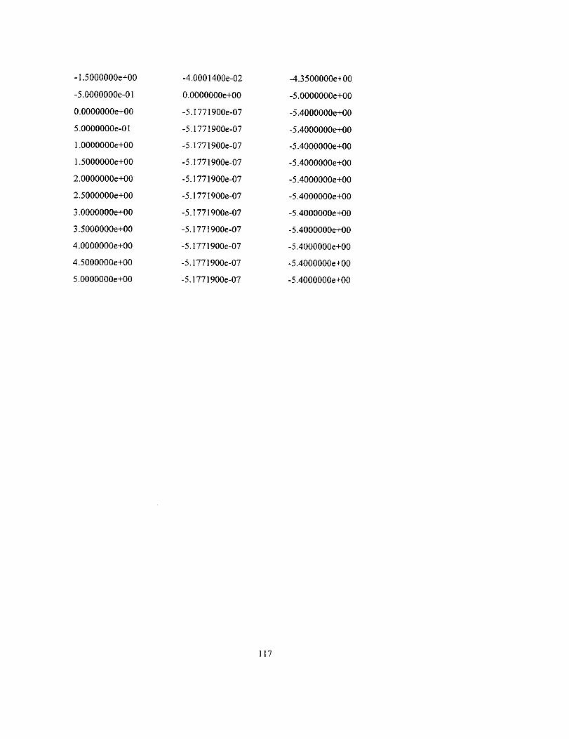
-l.5000000e+O0
-5.0000000e-Ol
O.O000000e+O0
5.0000000e-Of
l.O000000e+O0
1.5000000e+00
2.0000000e+O0
2.5000000e+00
3.0000000e+O0
3.5000000e+00
4.0000000e+O0
4.5000000e+00
5.0000000e+O0
-4.0001400e-02
O.O000000e+O0
-5.1771900e-07
-5.1771900e-07
-5.1771900e-07
-5.1771900e-07
-5.1771900e-07
-5.1771900e-07
-5.1771900e-07
-5.1771900e-07
-5.1771900e-07
-5.1771900e-07
-5.1771900e-07
-4.3500000e+00
-5.0000000e+O0
-5.4000000e+00
-5.4000000e+00
-5.4000000e+00
-5.4000000e+00
-5.4000000e+00
-5.4000000e+00
-5.4000000e+00
-5.4000000e+00
-5.4000000e+00
-5.4000000e+00
-5.4000000e+00
117
APPENDIX C
NON-CONSTANT ENVELOPE
SIMULATION
BLOCK DIAGRAM
This appendix contains a detailed diagram of the non-constant envelope simulation circuit used on
SPW to be able to measure the effect of the non-constant envelope through the SSPA. A brief
explanation of this circuit will be given.
Figure C.1 shows the detailed SPW diagram of the Non-Constant Envelope Simulations also
described in Figure 3.34 of section 3.4 in this report. Note the similarity of Figure C.1 with the
Figures in Appendix A. One of the only differences is the model of the SSPA which has been slightly
modified. In fact, Figure C.2 shows a detailed diagram of this new model of SSPA. This new model
was created to get a better rotation accuracy due to the AM/PM conversion in the SSPA. In this new
SSPA model, the SSPA table shown in Appendix B has been modified in the sense that two new tables
were created ,i.e., one table which was named "outdb.ascsig" contained the input dB column (first
column of the table in Appendix B) and the output dB (second column of table in Appendix B).
Therefore this first file was the AM/AM conversion created by the SSPA. The second file that was
created was called "outphase.ascsig" and contains the columns from the table in Appendix B that
produced the AM/PM conversion ,i.e., column i and 3.
Therefore the two TABULAR NON LINEAR blocks in Figure C.2 refer to these files to output the
corresponding amplitude or phase conversion. The highest TABULAR NON LINEAR block in the
figure refers to the "outdb.ascsig" table and the second block refers to the "outphase.ascsig" table.
The rest of the block diagram is self explanatory.
118
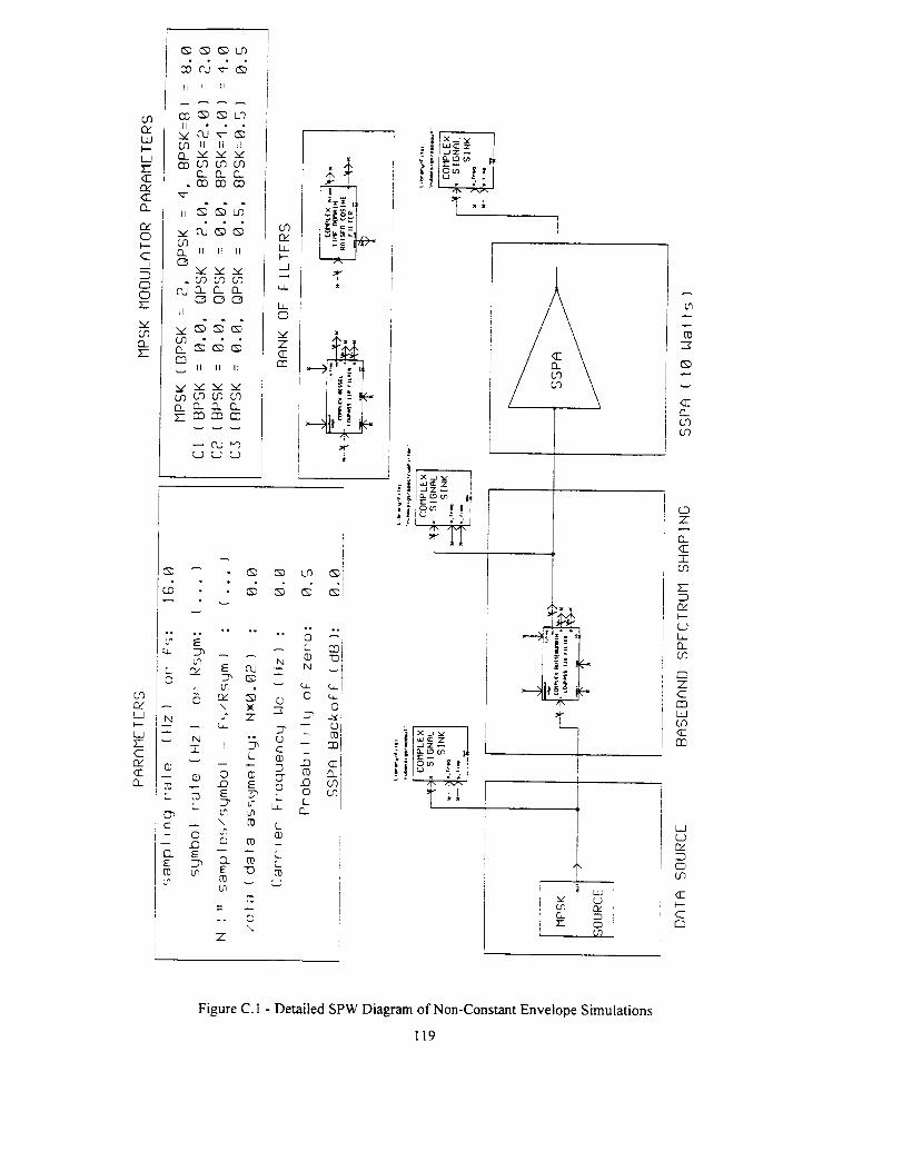
O'3n."
k.J21CryCG_
O3O_LOt---LJy.-
rFCO-
rv"C3
k--
C
CDCDy--
vcoo_z;-
_ _ eD t5)• • ° ,
c_ od _ eD
U II _1 ]1
If) It Ii HO. v v vCO CO Ct3 O3
O._ [2. 0... CO 00 CO
U3O_ II IE II
v v v
OdD-0-O..C_ C3 C_
H
ODII H II
U_._ v v vU3 C_ O0
y__ _.. 0.. O_rr_ F'n _
L.) k.3 C.._
j,,
c_
y
©
N"r
CO
C_L_
C_C
EC_
berv"
IN3-
CO
70L
or_E
be
_D
E
d
L
0 _..0 EE __ mm m
", mm
Ck _E "_
t_m
INZ
,°
c
L
LL
C.2
L_
d
f_
IN
ca_©
z_
L
Ii
g_
, r
t
<z
coco
(.DZ
C_CI09
Drw
L2L_0_C0
rmZC
09
r_
LJUrw
c_
ct.--
c
Figure C. 1 - Detailed SPW Diagram of Non-Constant Envelope Simulations
119
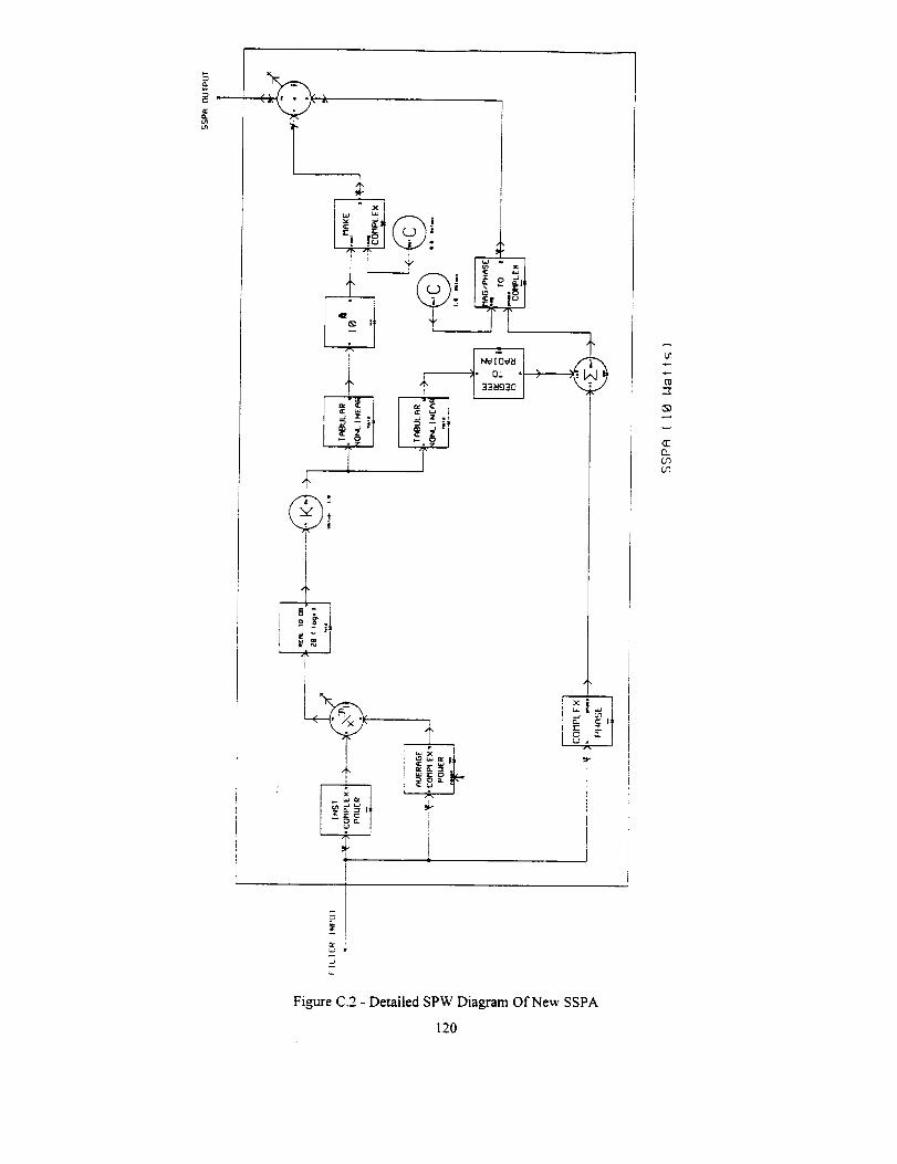
+
J
4,
A
C
u_
_1
Figure C.2 - Detailed SPW Diagram Of New SSPA
120
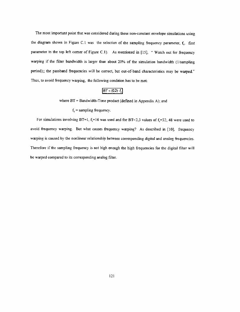
The most important point that was considered during these non-constant envelope simulations using
the diagram shown in Figure C. 1 was the selection of the sampling frequency parameter, fs, first
parameter in the top left comer of Figure C.1). As mentioned in [15], " Watch out for frequency
warping if the filter bandwidth is larger than about 20% of the simulation bandwidth (I/sampling
period);; the passband frequencies will be correct, but out-of-band characteristics may be warped."
Thus, to avoid frequency warping, the following condition has to be met:
Isr <(o.2>.q
where BT = Bandwidth-Time product (defined in Appendix A); and
f, = sampling frequency.
For simulations involving BT=I, f,=16 was used and for BT=2,3 values of f,=32, 48 were used to
avoid frequency warping. But what causes frequency warping? As described in [10], frequency
warping is caused by the nonlinear relationship between corresponding digital and analog frequencies.
Therefore if the sampling frequency is not high enough the high frequencies for the digital filter will
be warped compared to its corresponding analog filter.
121
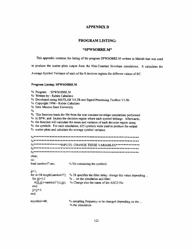
APPENDIX D
PROGRAM LISTING:
"SPWSOBRE.M"
This appendix contains the listing of the program SPWSOBRE.M written in Matlab that was used
to produce the scatter plots output from the Non-Constant Envelope simulations. It calculates the
Average Symbol Variance of each of the 8 decision regions for different values of BT.
Program Listing: SPWSOBRE.M
% Program : SPWSOBRE.M
% Written by : Ruben Caballero
% Developed using MATLAB V4.2B and Signal Processing Toolbox V3.0b% Copyright 1996 - Rub6n Caballero
% New Mexico State University%
% This function loads the file from the non-constant envelope simulations performed
% in SPW, and locates the decision region where each symbol belongs. Afterwards,
% the function will calculate the mean and variance of each decision region using
% the symbols. For each simulation, 625 symbols were used to produce the output% scatter plots and calculate the average symbol variance.
jj=l;
for ii=38:length(sambut 17);
for jjj=1:2
A(jj,jjj)=sambut 17(ii,jjj);end;
jj=jj+l ;end;
% 38 specifies the filter delay: change this value depending ...% ... on the simulation and filter
% Change also the name of the ASCII file
nsymbol=48; % sampling frequency to be changed depending on the ...% the simulation
122
[nr nc]=size(A);
for q= 1:nr
x(q)=A(q, 1)* (cos(A(q,2))+sin(A(q,2))* i);
end;
[nr nc]=size(x);
Ksymbols=floor(nc/nsymbol);
x=x( 1:Ksymbols*nsymbol);
z=[-l:O.Ol:l];
[rz nz]=size(z);
y=sqrt(ones(l,nz)-z.*z);
plot(z,y,'b-',z,-y,'b-');
grid
axis('square');
hold on;
% Create the axis for the Scatter Plot
avg=sum(abs(x));
avg=av_nc;
for i= 1:Ksymbols
m=(nsymbol)*i;
symbois(i)=x(m)/avg;end
% Determine the location of the symbols.
RxSig=angle(symbols);
dec0= 1;
decl =1 ;
dec2 = 1;
dec3= 1;
dec4= 1;dec5 = 1:
dec6 = 1;
dec7 = 1;
for i= I :length(RxSig) % Decision Region 0
if ((RxSig(i)>=0) & (RxSig(i) <=pi/4))decision0(dec0)=symbols(i);
dec0=dec0+ 1 ;
end;
123
if ((RxSig(i)>=pi/4)& (RxSig(i)<=pi/2))decision1(dec1)=symbols(i);decI=dec 1+ 1;
end;
if ((RxSig(i)>pi/2) & (RxSig(i) <=6"pi/8))
decision2(dec2)=symbols(i);dec2=dec2+ l;
end;
if ((RxSig(i)>=6*pi/8) & (RxSig(i) <=pi))decision3(dec3)=symbols(i);
dec3 =dec3 + 1;
end;
% Decision Region l
% Decision Region 2
% Decision Region 3
if ((RxSig(i)>-pi)& (RxSig(i) <= -6"pi/8))
decision4(dec4)=symbols(i);dec4=dec4+ 1;
end;
% Decision Region 4
if ((RxSig(i)>-6*pi/8) & (RxSig(i) <=-pi/2))
decision5(dec5)=symbols(i);
dec5=dec 5+ 1;
end;
% Decision Region 5
if ((RxSig(i)> -pi/2) & (RxSig(i) <=-pi/4))
decision6(dec6)=symbols(i);
dec6=dec6+ l;
end;
% Decision Region 6
if ((RxSig(i)>-pi/4) & (RxSig(i) <0))
decision7(dec7)=symbols(i);
dec7-dec7+ 1;
end;
% Decision Region 7
end; % end FOR
piot(symbols,'go');
axis([-1.25 +1.25 -1.25 +1.25]);
title('Output of SSPA (saturation level), 5th Order Butterworth Filter (BT=3.8)');
xlabel('rear);
ylabel('imag');% Calculation of the Mean of the Symbols in the Decision Regions
meanrad(1)=(mean(angle(decisionO)));
meandeg(l )=(meanrad(1 )* 180/pi);
meanrad(2)=(mean(angle(decisionl)));
meandeg(2)=(meanrad(2) * 180/pi);
% mean in rads
% mean in degrees
% mean in rads
% mean in degrees
124
meanrad(3)=(mean(angle(decision2)));meandeg(3)=(meanrad(3)*180/pi);
meanrad(4)=(mean(angle(decision3)));meandeg(4)=(meanrad(4)*180/pi);
meanrad(5)=(mean(angle(decision4)));meandeg(5)=(meanrad(5)*180/pi);
meanrad(6)=(mean(angle(decision5)));meandeg(6)=(meanrad(6)*180/pi);
meanrad(7)=(mean(angle(decision6)));meandeg(7)=(meanrad(7)*180/pi);
meanrad(8)=(mean(angle(decision7)));meandeg(8)=(meanrad(8)*180/pi);
% mean in rads
% mean in degrees
% mean in rads
% mean in degrees
% mean in rads
% mean in degrees
% mean in rads
% mean in degrees
% mean in rads
% mean in degrees
% mean in rads
% mean in degrees
% Calculation of the Variance of the Symbols in the Decision Regions
varrad(l )=(std(angle(decision0))).^2; % variance in rads
vardeg(1)=(varrad(1)* 180/pi); % variance in degrees
varrad(2)=(std(angle(decisionl))).^2; % variance in rads
vardeg(2)=(varrad(2)* 180/pi); % variance in degrees
varrad(3)=(std(angle(decision2)))."2; % variance in rads
vardeg(3)=(varrad(3) * 180/pi); % variance in degrees
varrad(4)=(std(angle(decision3))).^2; % variance in rads
vardeg(4)=(varrad(4) * 180/pi); % variance in degrees
varrad(5)=(std(angle(decision4))).^2; % variance in fads
vardeg(5)=(varrad(5)* 180/pi); % variance in degrees
varrad(6)=(std(angle(decision5))).^2" % variance in rads
vardeg(6)=(varrad(6)* 180/pi); % variance in degrees
varrad(7)=(std(angle(decision6))).^2; % variance in rads
vardeg(7)=(varrad(7)* 180/pi); % variance in degrees
varrad(8)=(std(angle(decision7))).^2;
vardeg(8)=(varrad(8) * 180/pi);
save meandeg; save vardeg;
time=(toc/60); % in minutes
% variance in rads
% variance in degrees
125
APPENDIX E
SCATTER PLOTS:
5Tn Order BUTTERWORTH FILTER
This appendix contains the Scatter Plots of the output of the SSPA when a 5th Order Butterworth
Spectrum Filter is used after the 8PSK Modulator. The Scatter Plots were produced for BT=I to 4
using the SPWSOBRE.M function. Also, the listing of the program BUTTPLOT.M written in Matlab
which was used to produce the Average Symbol Variance plots (see Figure 3.43 and 3.44 in this
report) is included. All the values of mean and variance in this program were calculated in the
program SPWSOBRE.M.
E.I Scatter Plots
126
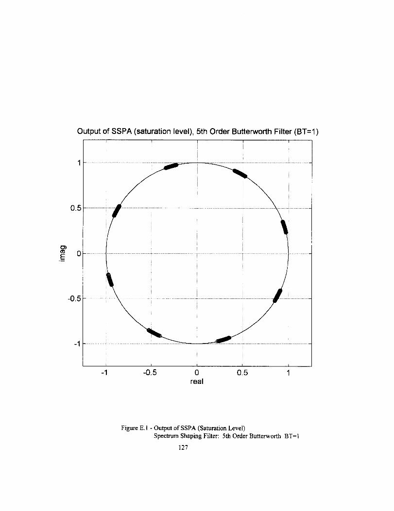
Output of SSPA (saturation level), 5th Order Butterworth Filter (BT=I)
{J)
E
05
111111111111111iiI iiiiiiiiiill_........................................................................ _....................................................
]
I I
-1 -0.5 0
real
0.5 1
Figure E.I - Output of SSPA (Saturation Level)
Spectrum Shaping Filter: 5th Order Butterworth BT=I
127
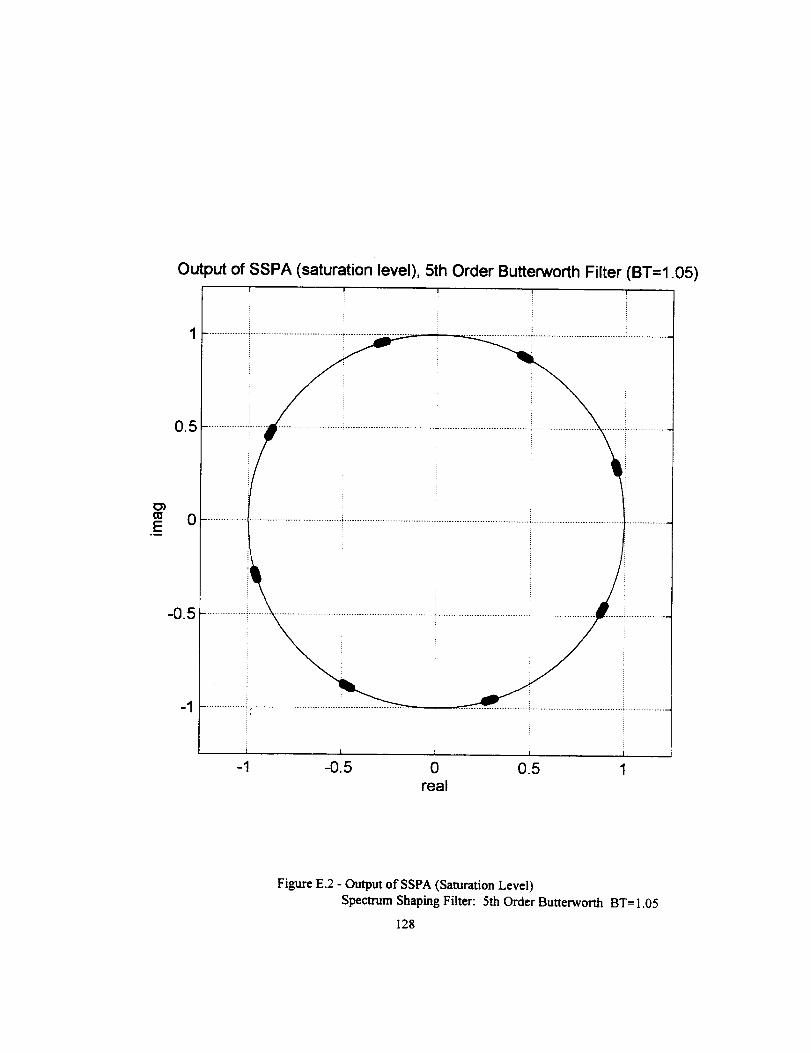
O)
E°_
Out
0.5
0
-0.5
-1
aut of SSPA (saturation level), 5th Order Butterworth Filter (BT=1.05)t !
i I I
-1 -0.5 0 0.5real
Figure E.2 - Output of SSPA (Saturation Level)
Spectrum Shaping Filter: 5th Order Butterworth BT=I.05
128
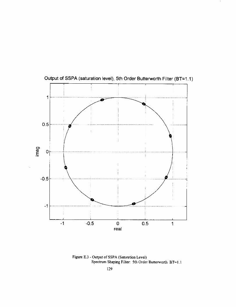
E
0.5
Output of SSPA (saturation level), 5th Order Butterworth Filter (BT=1.1)I I
0
i "I 1
-1 -0.5 0 0.5 1
real
-0.5
-1
Figure E.3 - Output of SSPA (Saturation Level)
Spectrum Shaping Filter: 5th Order Butterworth BT=I.I
129
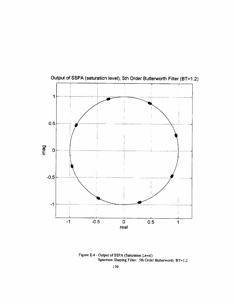
Output of SSPA (saturation level), 5th Order Butterworth Filter (BT=1.2)
E°_
-1 -0.5 0 0.5 1real
Figure E.4 - Output of SSPA (Saturation Level)
Spectrum Shaping Filter: 5th Order Butterworth BT= 1.2
130
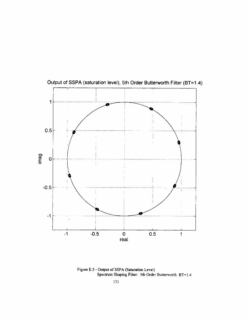
Output of SSPA (saturation level), 5th Order Butterworth Filter (BT=I.4)
{31)
E°_
0.5
0
-0.5
-1
-1 -O.5 0 0.5 1real
Figure E.5 - Output of SSPA (Saturation Level)
Spectrum Shaping Filter: 5th Order Butterwonh BT=1.4
131
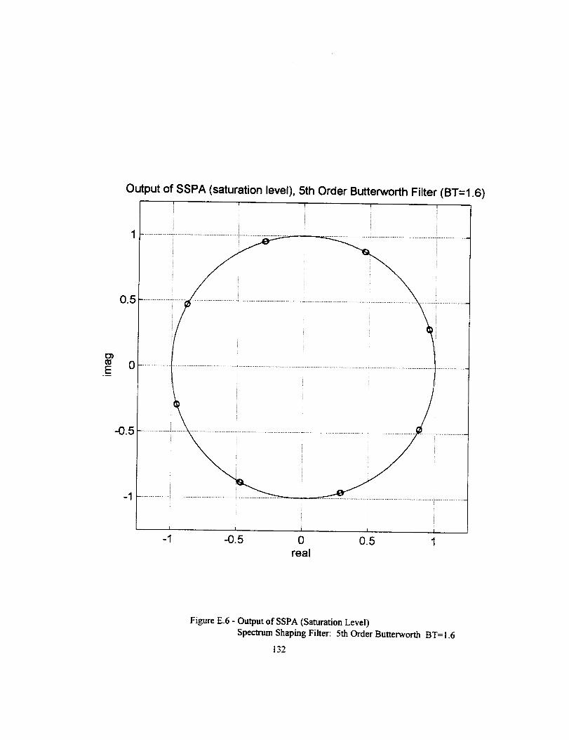
Output of SSPA (saturation level), 5th Order Butterworth Filter (BT=1.6)
O0E
0.5
................................................... _.................................... ......................................................................................
o51i iI I I I
-1 -0.5 0 1real
i
0.5
Figure E.6 - Output of SSPA (Saturation Level)
Spectrum Shaping Filter: 5th Order Butterworth BT=1.6
132
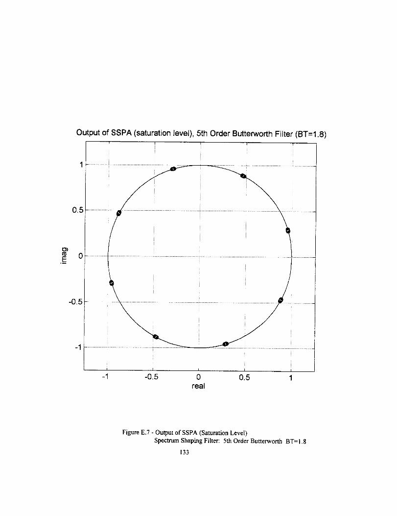
E°_
0.5
Output of SSPA (saturation level), 5th Order Butterworth Filter (BT=1.8)I
-05
-1
................
-1 -0.5 0 0.5 1real
Figure E.7 - Output of SSPA (Saturation Level)
Spectrum Shaping Filter: 5th Order Butterworth BT=1.8
133
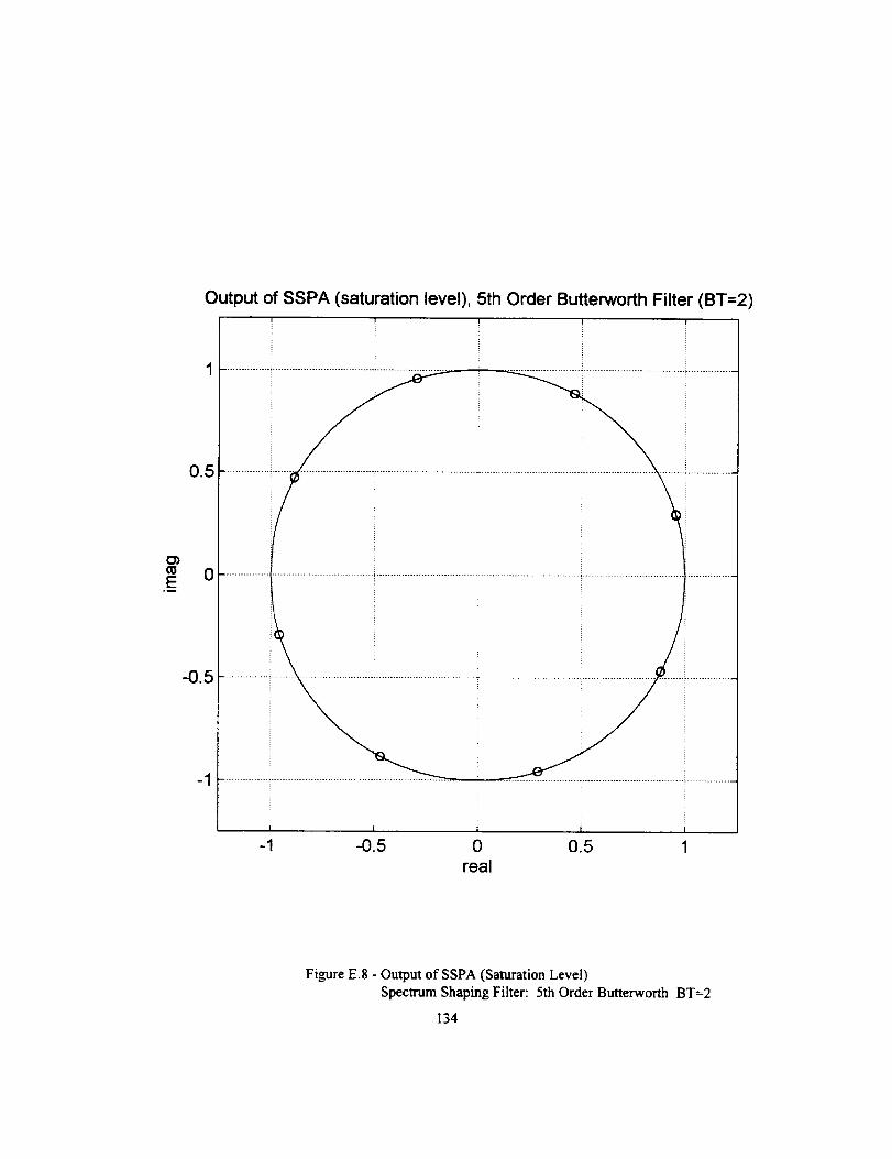
O)
Eo--
0.5
Output of SSPA (saturation level), 5th Order Butterworth Filter (BT=2)! i
0
-0.5
-1
i i i i-1 -0.5 0 0.5 1
real
Figure E.$ - Output of SSPA (Saturation Level)
Spectrum Shaping Filter: 5th Order Butterworth BT=2
134
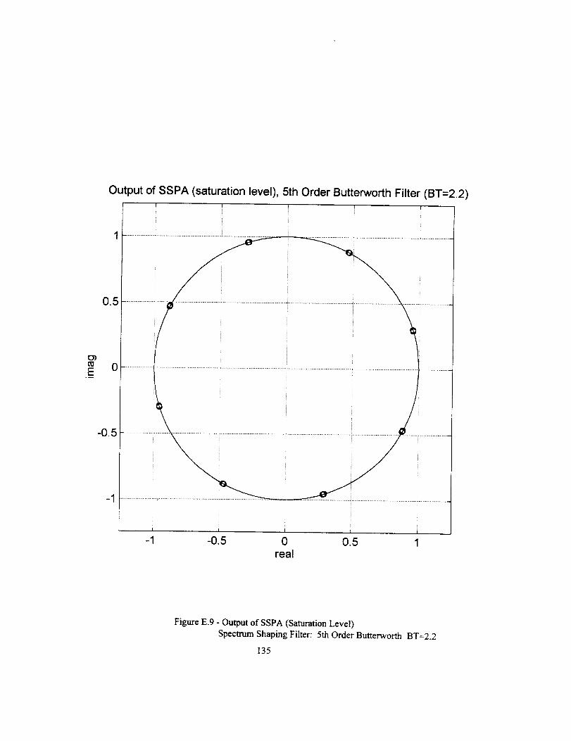
Output of SSPA (saturation level), 5th Order Butterworth Filter (BT=2.2)
{33
E
-1 -0.5 0 0.5 1real
Figure E.9 - Output of SSPA (Saturation Level)
Spectrum Shaping Filter: 5th Order Butterworth BT=2.2
135
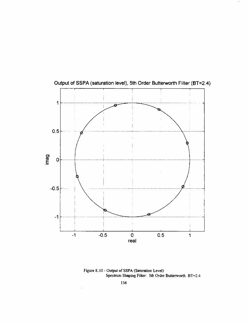
E°D
Output of SSPA (saturation level), 5th Order Butterworth Filter (BT=2.4)
0.5
0
-0.5
-1
I I I I I
-1 -O.5 0 O.5 1real
Figure E. 10 - Output of SSPA (Saturation Level)
Specla-um Shaping Filter: 5th Order Butterworth BT=2.4
136
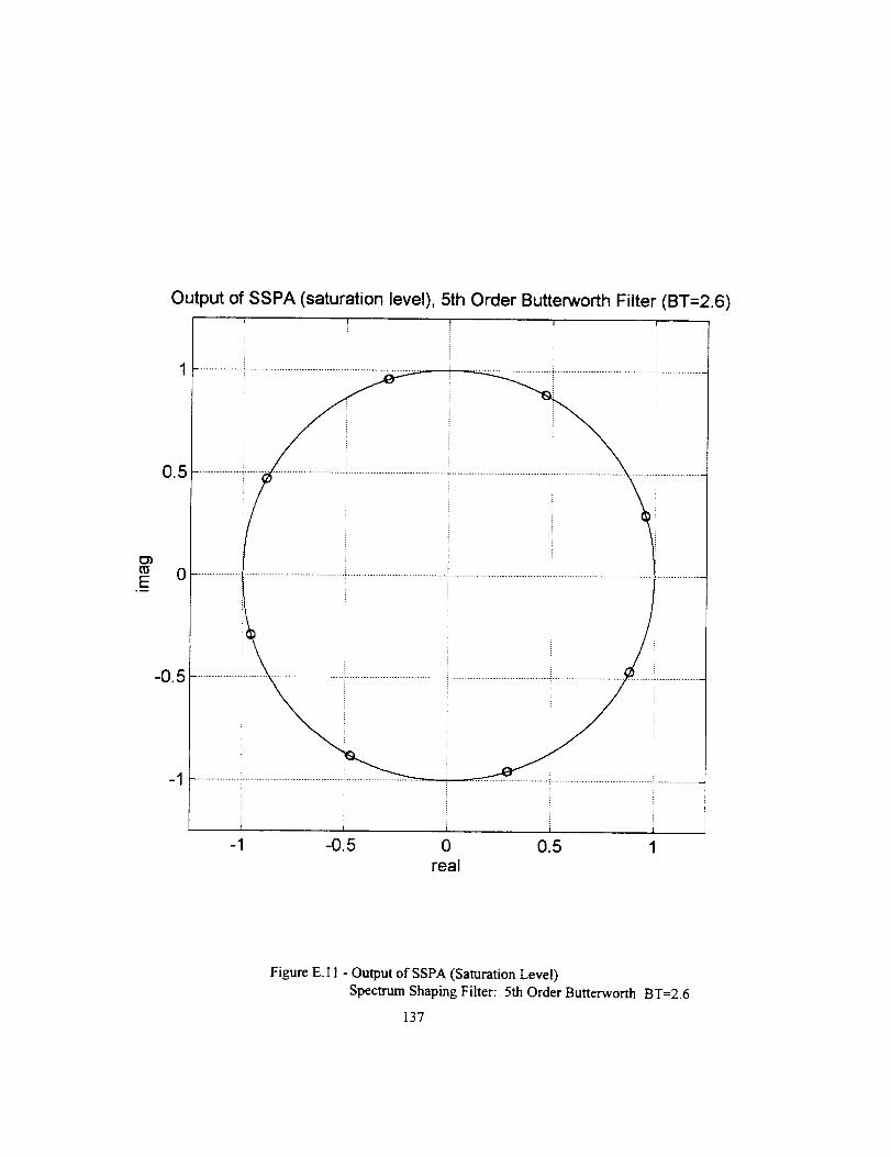
Output of SSPA (saturation level), 5th Order Butterworth Filter (BT=2.6)
E°_
r [
-1 -0.5 0 0.5 1real
Figure E. l 1 - Output of SSPA (Saturation Level)
Spectrum Shaping Filter: 5th Order Butterworth BT=2.6
137
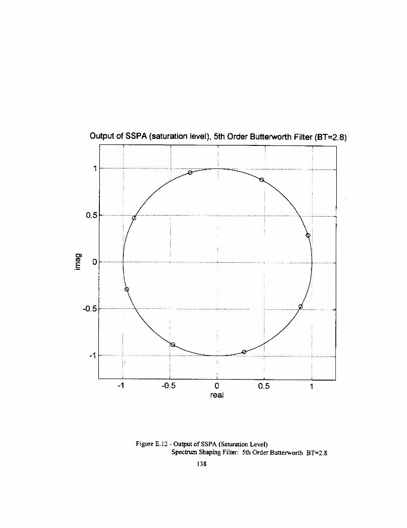
E
0.5
-0.5_
Output of SSPA (saturation level), 5th Order Butterworth Filter (BT=2.8)
=:
O ................................................... , .................................... • .................................. ...................................................
,I-= : - .............................................. i ................
i i-1 -0.5 0 0.5 1
real
Figure E. 12 - Ou_ut of SSPA (Saturation Level)
Spectrum Shaping Filter: 5th Order Butterworth BT=2.8
138
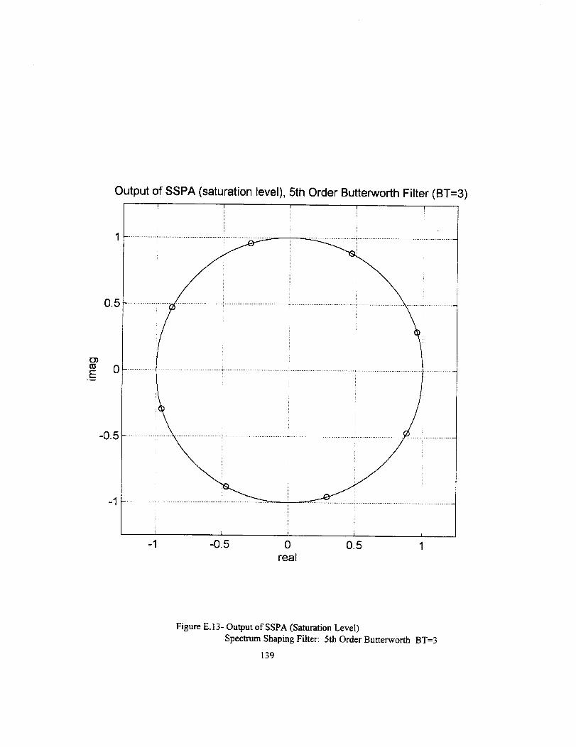
Output of SSPA (saturation level), 5th Order Butterworth Filter (BT=3)
_3b
E°_
0.5
0
-0.5
-1
iiiiiiiiiiiii!i iliii....................................................i...........................................................................................................................
J i-1 -0.5 0 0.5 1
real
Figure E. 13- Output of SSPA (Saturation Level)
Spectrum Shaping Filter: 5th Order Butterworth BT=3
139
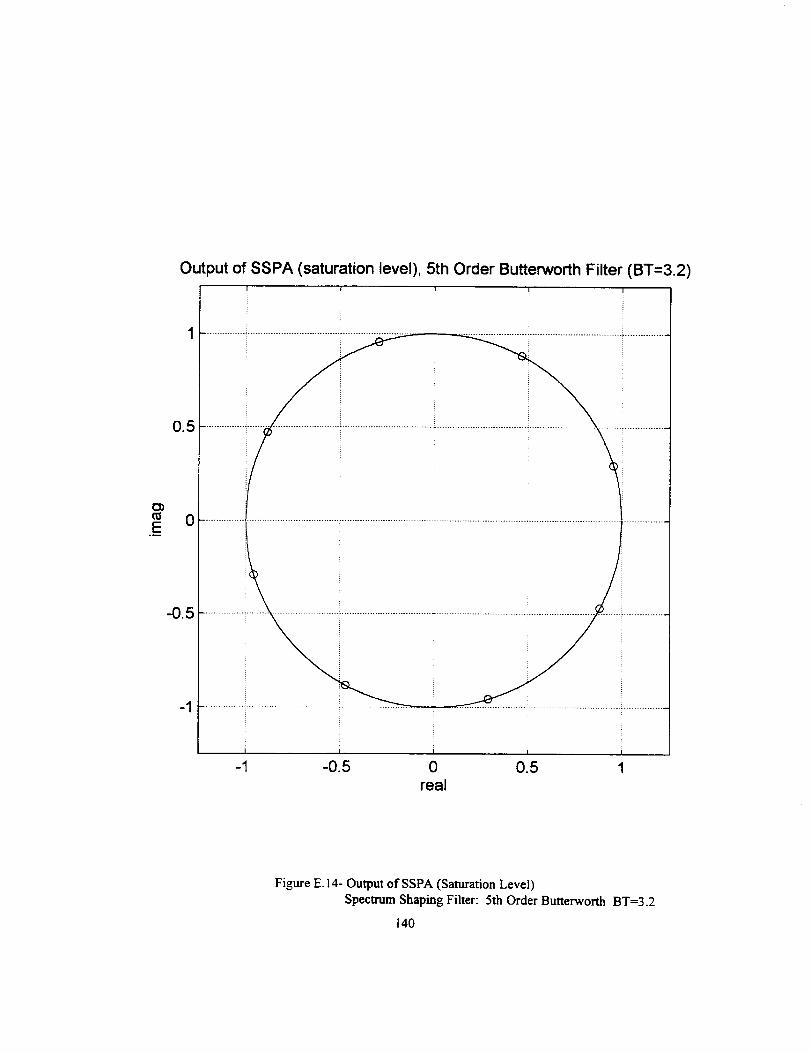
Output of SSPA (saturation level), 5th Order Butterworth Filter (BT=3.2)
O)¢0E
0.5
0
-0.5
-1
-1 -0.5 0 0.5 1real
Figure E. 14- Output of SSPA (Saturation Level)
Spectrum Shaping Filter: 5th Order Butterworth BT=3.2
140
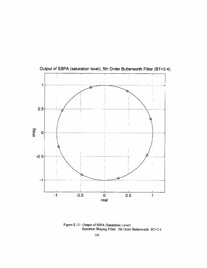
O')
E.m
Output of SSPA (saturation level), 5th Order Butterworth Filter (BT=3.4)
i.................................................. , ..........................................................................................................................
I I i I
-1 -0.5 0 0.5 1
real
0.5
-0.5i
Figure E. 15 - Output of SSPA (Saturation Level)
Spectrum Shaping Filter: 5th Order Butterworth BT=3.4
141
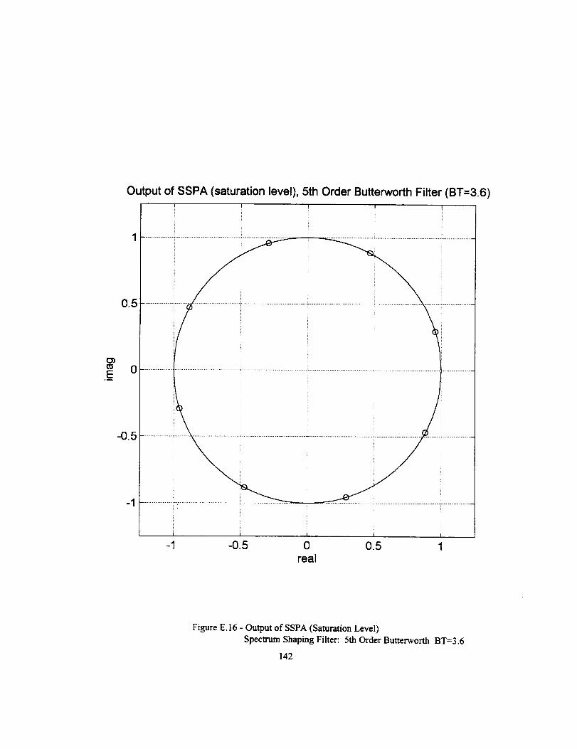
Output of SSPA (saturation level), 5th Order Butterworth Filter (BT=3.6)
E°__
Figure E. 16 - Output of SSPA (Saturation Level)
Spectrum Shaping Filter: 5th Order Butterworth BT=3.6
142
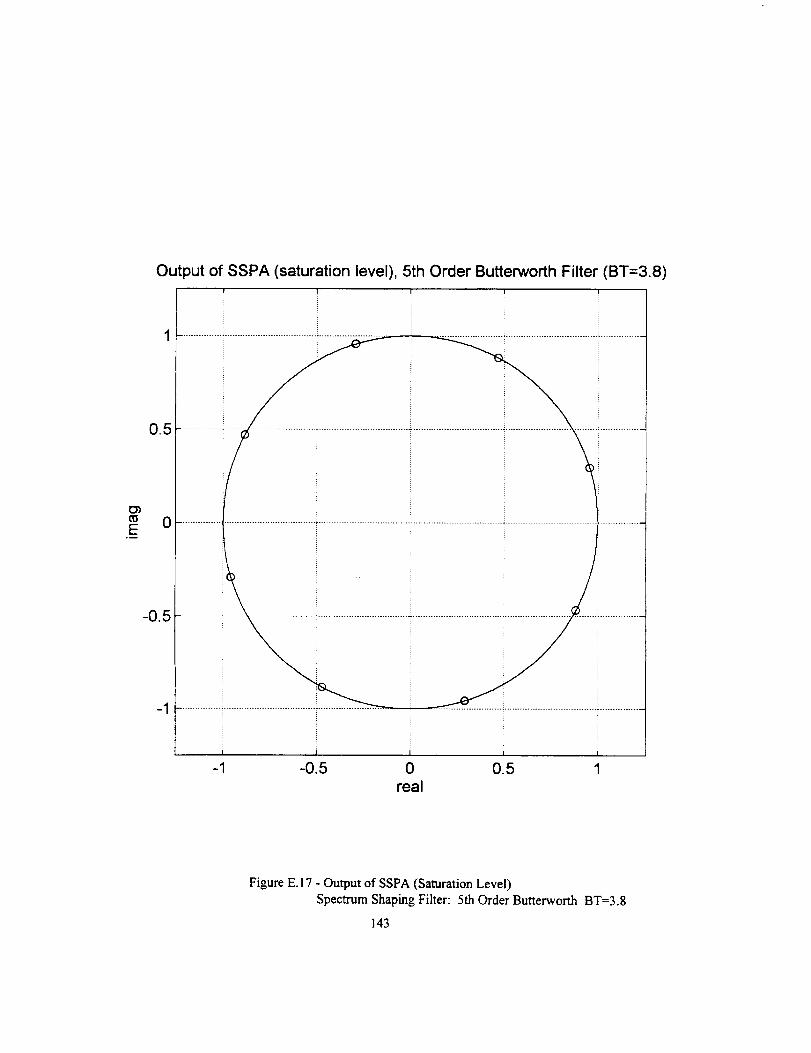
Output of SSPA (saturation level), 5th Order Butterworth Filter (BT=3.8)
Cr}
EoD
0.5
0
-0.5
-1
t i t i
-1 -0.5 0 0.5 1real
Figure E. I 7 - Output of SSPA (Saturation Level)
Spectrum Shaping Filter: 5th Order Butterworth BT=3.8
143
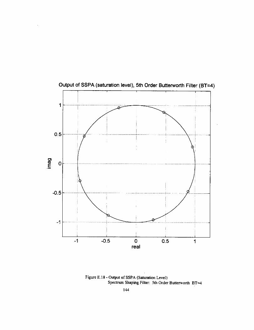
Output of SSPA (saturation level), 5th Order Butterworth Filter (BT=4)
E.m
0.5
0
-0.5
-1
Figure E. 18 - Output of SSPA (Saturation Level)
Spectrum Shaping Filter: 5th Order Butterworth BT=4
144
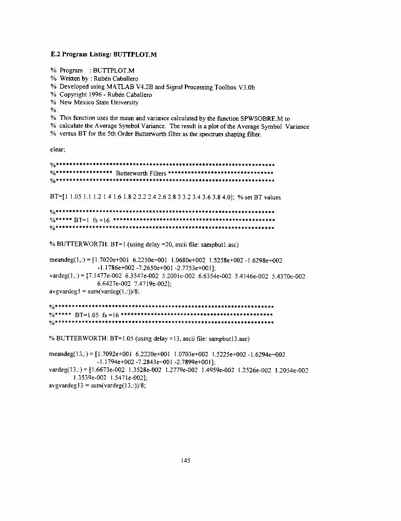
E.2 Program Listing: BUTTPLOT.M
% Program : BUTTPLOT.M
% Written by : Rub6n Caballero
% Developed using MATLAB V4.2B and Signal Processing Toolbox V3.0b% Copyright 1996 - Ruben Caballero
% New Mexico State University%
% This function uses the mean and variance calculated by the function SPWSOBRE.M to
% calculate the Average Symbol Variance. The result is a plot of the Average Symbol Variance
% versus BT for the 5th Order Butterworth filter as the spectrum shaping filter.
clear;
BT=[I 1.05 1.1 1.2 1.4 1.6 1.8 2 2.2 2.4 2.6 2.8 3 3.2 3.4 3.6 3.8 4.0]; % set BT values
% BUTTERWORTH: BT=I (using delay =20, ascii file: sampbutl.asc)
meandeg(1,:) = [1.7020e+001 6.2250e+001 1.0680e+002 1.5258e+002-1.6298e+002
-1.1786e+002 -7.2650e+001-2.7753e+001];
vardeg(1,:) = [7.1477e-002 6.3547e-002 5.2001e-002 6.6354e-002 5.4146e-002 5.4370e-002
6.6427e-002 7.4719e-002];
avgvardegl = sum(vardeg(1,:))/8;
% BUTTERWORTH: BT= 1.05 (using delay = 13, ascii file: sampbut 13.asc)
meandeg(13,:) = [1.7092e+001 6.2220e+001 1.0703e+002 1.5225e+002-1.6294e+002-1.1794e+002-7.2843e+001-2.7899e+001];
vardeg(13,:) = [1.6673e-002 1.3528e-002 1.2779e-002 1.4959e-002 1.2526e-002 1.2054e-002
1.3539e-002 1.5471e-002];
avgvardegl3 = sum(vardeg(13,:))/8;
145
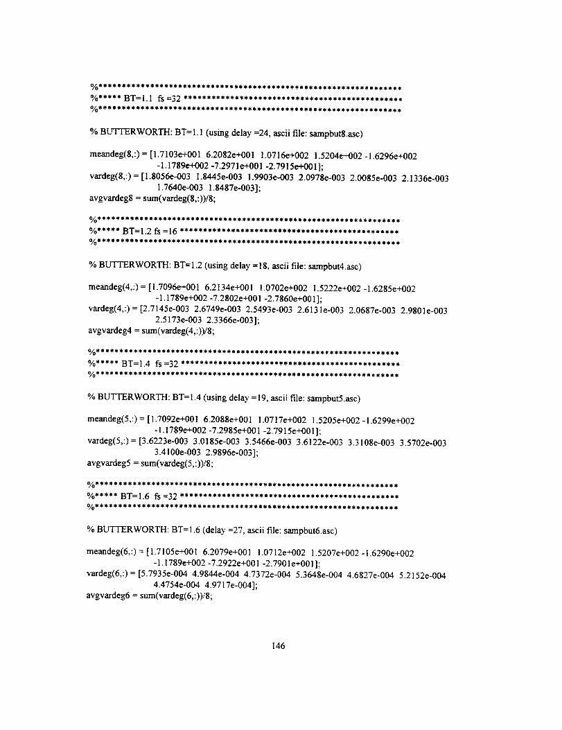
%BUTTERWORTH:BT=I.1(usingdelay=24,asciifile:sampbut8.asc)
meandeg(8,:) = [1.7103e+001 6.2082e+001 !.0716e+002 1.5204e+002 -1.6296e+002
-1.1789¢+002-7.2971e+001-2.7915e+001];
vardeg(8,:) = [1.8056¢-003 1.8445e-003 1.9903e-003 2.0978e-003 2.0085e-003 2.1336e-003
1.7640e-003 1.8487e-003];avgvardeg8 = sum(vardeg(8,:))/8;
% BUTTERWORTH: BT--1.2 (using delay = 18, ascii file: sampbut4.asc)
meandeg(4,:) = [1.7096e+001 6.2134e+001 1.0702e+002 1.5222e+002 -1.6285e+002
-1.1789e+002 -7.2802e+001 -2.7860e+001];vardeg(4,:) = [2.7145e-003 2.6749e-003 2.5493e-003 2.6131e-003 2.0687e-003 2.9801e-003
2.5173e-003 2.3366e-003];
avgvardeg4 = sum(vardeg(4,:))/8;
% BUTTERWORTH: BT= 1.4 (using delay = 19, ascii file: sampbut5.asc)
meandeg(5,:) = [1.7092e+001 6.2088e+001 1.0717e+002 1.5205e+002-1.6299e+002
-1.1789e+002-7.2985e+001-2.7915e+001];vardeg(5,:) = [3.6223e-003 3.0185e-003 3.5466e-003 3.6122e-003 3.3108e-003 3.5702e-003
3.4100e-003 2.9896e-003];avgvardeg5 = sum(vardeg(5,:))/8;
% BUTTERWORTH: BT=1.6 (delay =27, ascii file: sampbut6.asc)
meandeg(6,:)= [1.7105e+001 6.2079e+001 1.0712e+002 1.5207e+002-1.6290e+002
- 1.1789e+002 -7.2922e+001 -2.7901 e+001 ];vardeg(6,:) = [5.7935e-004 4.9844e-004 4.7372e-004 5.3648e-004 4.6827e-004 5.2152e-004
4.4754e-004 4.9717e-004];
avgvardeg6 = sum(vardeg(6,:))/8;
146
%BUTTERWORTH:BT=I.8(delay=35,asciifile:sampbut7.asc)
meandeg(7,:)= [1.7103e+0016.2156e+0011.0708e+0021.5217e+002-1.6291e+002- 1.1791 e+002 -7.2871 e+001 -2.7893e+001 ];
vardeg(7,:) = [3.0054e-003 2.4409e-003 2.3048e-003 2.7448e-003 2.2233e-003 2.1648e-003
2.4702e-003 2.8097e-003];
avgvardeg7 = sum(vardeg(7,:))/8;
%BUTTERWORTH: BT=2 (using delay = 32, ascii file: sampbut2.asc)
meandeg(2,:) = [1.7100e+001 6.211 le+001 1.0710e+002 1.521 le+002 -1.6290e+002 -
1.1790e+002 -7.2897e+001 -2.7899e+001 ];vardeg(2,:) = [1.2757e-004 1.0112e-004 9.9469e-005 1.1625e-004 9.3600e-005 8.5729e-005
1.0797e-004 1.2218e-004];
avgvardeg2 = sum(vardeg(2,:))/8;
%BUTTERWORTH: BT=2.2 (using delay = 29, ascii file: sampbut9.asc)
meandeg(9,:) = [1.7098e+001 6.2134e+001 1.0707e+002 1.5215e+002-1.6289e+002
-1.1791e+002 -7.2870e+001-2.7895e+001];
vardeg(9,:) = [1.1019e-003 9.3545e-004 8.7686e-004 1.0168e-003 8.5896e-004 9.3158e-004
8.5970e-004 9.7456e-004];
avgvardeg9 = sum(vardeg(9,:)y8;
%BUTTERWORTH: BT=2.4 (using delay = 27, ascii file: sambutl 0.asc)
meandeg(10,:) = [1.7080e+001 6.2064e+001 1.0709e+002 1.5206e+002 -1.6292e+002
-1.1792e+002-7.2927e+001-2.7922e+001];
vardeg(10,:) = [2.5908e-004 2.1067e-004 2.0091e-004 2.3544e-004 1.9016e-004 1.8373e-004
2.0921e-004 2.4034e-004];
avgvardegl0 = sum(vardeg(10,:))/8;
147
%BUTTERWORTH:BT=2.6(usingdelay=34,asciifile:sambutll.asc)
meandeg(ll,:)= [1.7076e+0016.2055e+0011.0709e+0021.5205e+002-1.6293e+002-1.1792e+002-7.2940e+001-2.7928e+001];
vardeg(ll,:)= [3.9346e-0043.3146e-0043.0956e-0043.6135e-0043.0312e-0043.1763e-0043.0654e-0043.5248e-004];
avgvardegll= sum(vardeg(ll,:))/8;
%BUTTERWORTH:BT=2.8(usingdelay=32,asciifile:sambutl2.asc)
meandeg(12,:)= [1.7078e+0016.2083e+0011.0708e+0021.5209e+002-1.6292e+002-1.1792e+002-7.2917e+001-2.7921e+001];
vardeg(12,:)= [1.4141e-0051.2143e-0051.2144e-0051.3224e-0051.I092e-0051.2642e-0051.1685e-0051.2637e-005];
avgvardegl2=sum(vardeg(12,:))/8;
%BUTTERWORTH:BT=3(usingdelay=30,asciifile: sampbut3.asc)
meandeg(3,:) = [1.7077e+001 6.2088e+001 1.0707e+002 1.5209e+002-1.6292e+002
-1.1792e+002-7.2913e+001-2.7921e+001];vardeg(3,:) = [9.9154e-005 8.3102e-005 7.9266e-005 9.1259e-005 7.4914e-005 8.1407e-005
7.9067e-005 8.9380e-005];avgvardeg3 = sum(vardeg(3,:))/8;
%BUTTERWORTH: BT=3.2 (using delay = 28, ascii file: sambutl4.asc)
meandeg(14,:) = [1.7072e+001 6.2073e+001 1.0707e+002 !.5207e+002 -1.6293e+002
-1.1793e+002 -7.2927e+001 -2.7928e+001];
vardeg(14,:)= [5.8964e-007 5.0913e-007 9.2412e-007 6.3686e-007 6.4852e-007 4.5768e-0071.0022e-006 5.8489e-007];
avgvardegl4 = sum(vardeg(14,:))/8;
148
%BUTTERWORTH:BT=3.4(usingdelay= 34,asciifile:sambutl5.asc)
meandeg(15,:)= [1.7069e+0016.2062e+0011.0707e+0021.5206e+002-1.6293e+002-1.1793e+002-7.2936e+001-2.7932e+001];
vardeg(15,:)=[4.8152e-0054.0562e-0053.7986e-0054.4103e-0053.8410e-0053.8316e-0053.7664e-0054.3210e-005];
avgvardegl5=sum(vardeg(15,:))/8;
%BUTTERWORTH:BT=3.6(usingdelay= 32,asciifile:sambutl6.asc)
meandeg(16,:)= [1.7068e+0016.2064e+0011.0707e+0021.5206e+002-1.6293e+002-1.1793e+002-7.2934e+001-2.7933e+001];
vardeg(16,:)=[1.6145e-0051.3681e-0051.2928e-0051.4785e-0051.3520e-0051.2891e-0051.2778e-0051.4431e-005];
avgvardegl6=sum(vardeg(16,:))/8;
%BUTTERWORTH:BT=3.8(usingdelay=37,asciifile:sambutl7.asc)
meandeg(17,:)= [1.7068e+0016.2071e+0011.0707e+0021.5207e+002-1.6293e+002-1.1793e+002-7.2929e+001-2.7932e+001];
vardeg(17,:)= [6.0818e-0065.0583e-0065.1543e-0065.6452e-0064.5621e-0064.9250e-0065.5862e-0065.5223e-006];
avgvardegl7= sum(vardeg(17,:))/8;
%BUTTERWORTH:BT=4.0(usingdelay=35,asciifile:sambutl8.asc)
meandeg(18,:)=[1.7067e+0016.2068e+0011.0707e+0021.5207e+002-1.6293e+002-1.1793e÷002-7.2932e+001-2.7933e+001];
vardeg(18,:)= [6.3159e-0075.2962e-0077.6612e-0076.0844e-0077.0038e-0075.1824e-0071.1054e-0065.8058e*007];
avgvardegl8=sum(vardeg(18,:))/8;
149
O_************ ********* 8., _****** *********
%****************** PLOTS***************
% Average Variance for the Symbols Plot
figure(I);
whitebg;
AMPMavgvar = [avgvardegl avgvardegl 3 avgvardeg8 avgvardeg4 avgvardeg5 avgvardeg6
avgvardeg7 avgvardeg2 avgvardeg9 avgvardeg 10 avgvardegl 1 avgvardegl 2
avgvardeg3 avgvardeg 14 avgvardeg 15 avgvardeg 16 avgvardeg 17 avgvardeg 18];
% interpolation using spline fit
interBT = 1:0.01:4.0;
interpol=spline(BT,AMPMavgvar,interBT);
plot(BT,AMPMavgvar,'ok',interBT, interpol,'k');
title('5th Order Butterworth Filter Symbol Average Variance vs BT');xlabel('Bandwidth-Time Product (BT)');
ylabei(' Variance in Degrees');
150

APPENDIX F
SCATTER PLOTS:
3 RDOrder BESSEL FILTER
This appendix contains the Scatter Plots of the output of the SSPA when a 3rd Order Bessel
Spectrum Filter is used after the 8PSK Modulator. The Scatter Plots were produced for BT=I to 4
using the SPWSOBRE.M function. Also, the listing of the program BESSPLOT.M written in Matlab
which was used to produce the Average Symbol Variance plots (see Figure 3.45 and 3.46 in this
report) is included. All the values of mean and variance in this program were calculated in the
program SPWSOBREM.
F.1 Scatter Plots
151
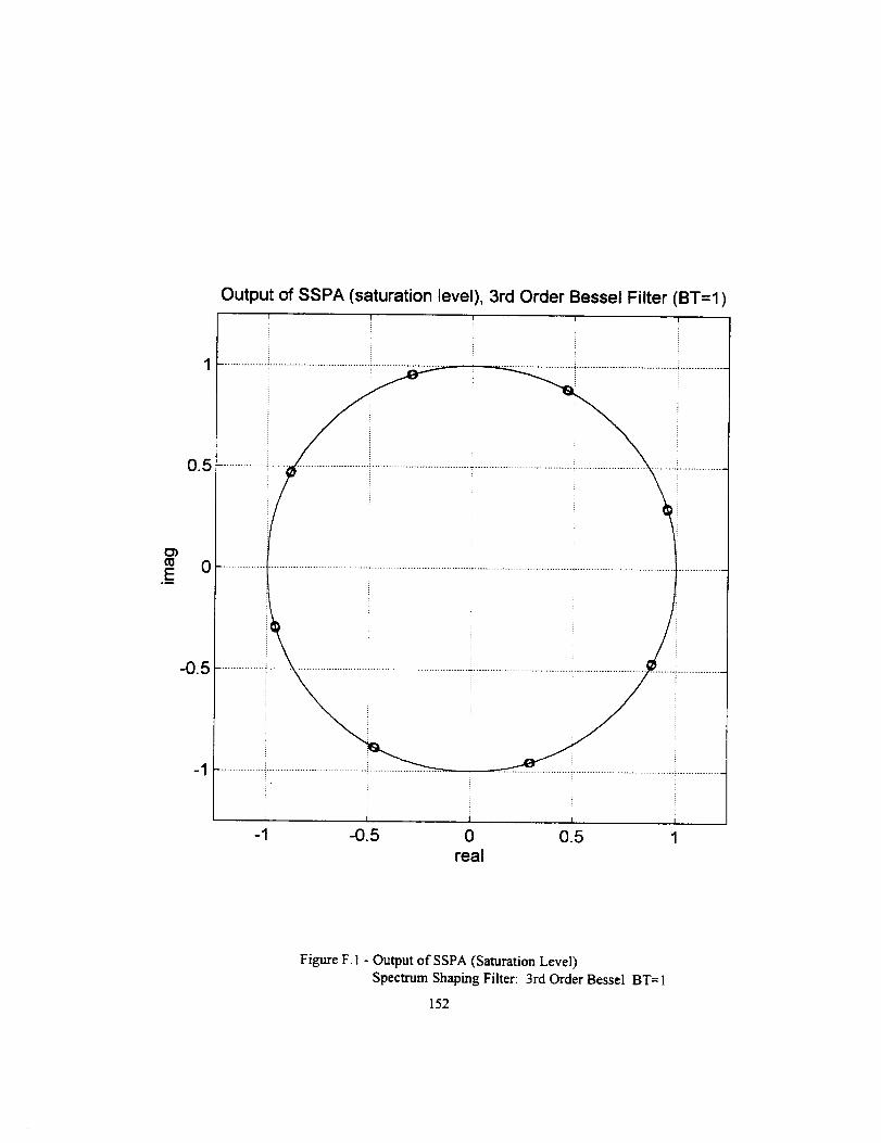
Output of SSPA (saturation level), 3rd Order Bessel Filter (BT=I
13)00E
0.5
0
-05
-1
-1 -0.5 0 0.5real
Figure F. 1 - Output of SSPA (Saturation Level)
Spectrum Shaping Filter: 3rd Order Bessel BT= 1
152
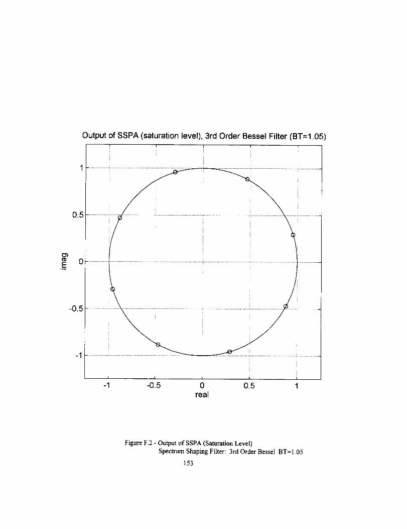
Output of SSPA (saturation level), 3rd Order Bessel Filter (BT=1.05)
Eom
0.5
0
-0.5
-1
Figure F.2 - Output of SSPA (Saturation Level)
Spectrum Shaping Filter: 3rd Order Bessel BT=1.05
153

mE
°D
0.5
0
-0.5
-1
i
L
Output of SSPA (saturation level), 3rd Order Bessel Filter (BT=1.1'I I I i I
I
-' -0.5 0 0.5 1real
Figure F.3 - Output of SSPA (Saturation Level)
Spectrum Shaping Filter: 3rd Order Bessel BT=I. 1
154
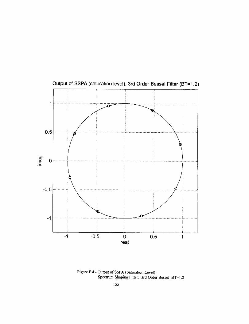
Output of SSPA (saturation level), 3rd Order Bessel Filter (BT=I.2
E.b
0.5
0
-05
-1
-1 -0.5 0 0.5 1real
Figure F.4 - Output of SSPA (Saturation Level)
Spectrum Shaping Filter: 3rd Order Bessel BT=I.2
155
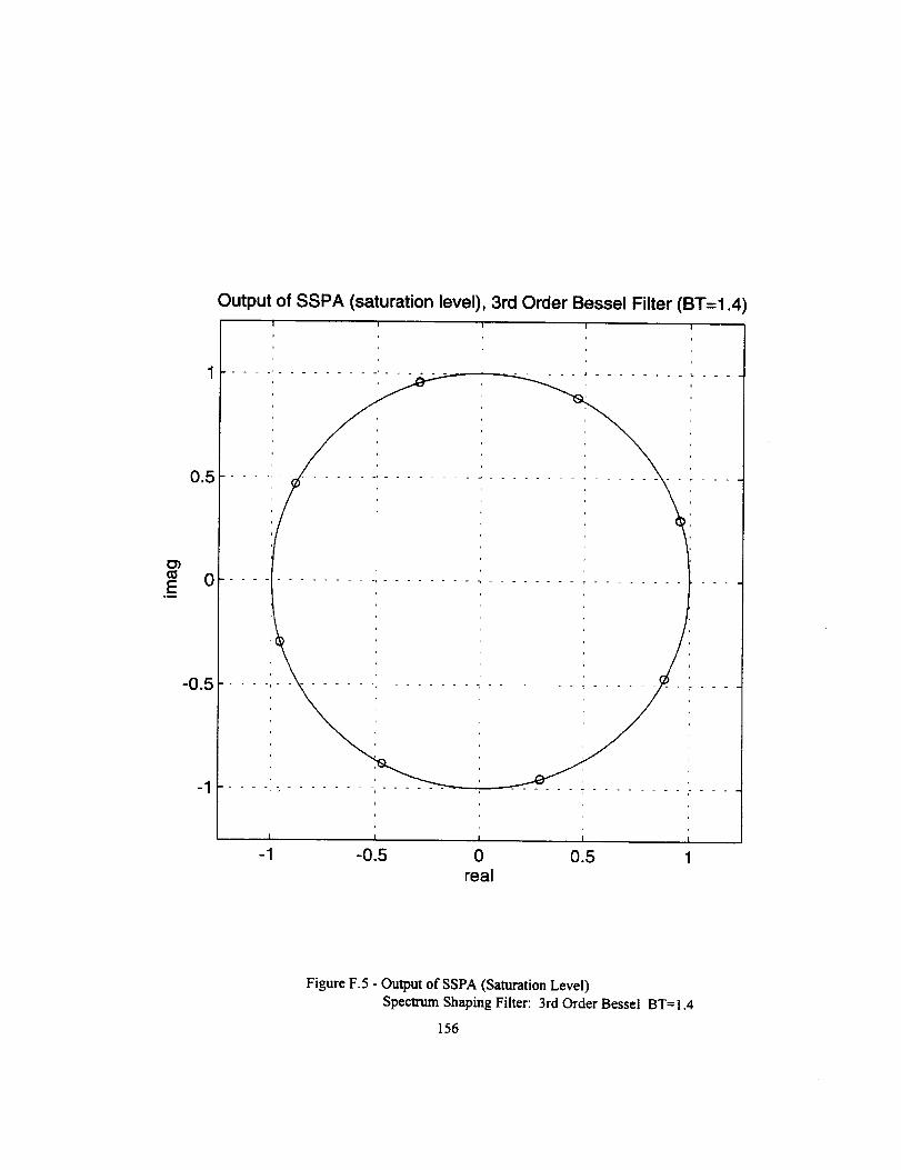
o_E
°_
0.5
0
-0.5
-1
Output of SSPA (saturation level), 3rd Order Bessel Filter (BT=1.4)I I I I I
Figure F.5 - Output of SSPA (Saturation Level)
Spectrum Shaping Filter: 3rd Order Bessel BT=I.4
156
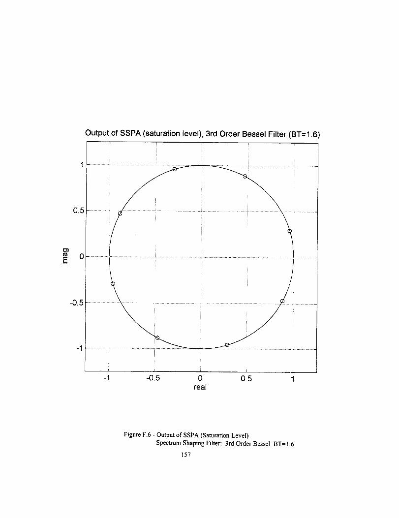
E.m
0.5
0
-05
-1
Output of SSPA (saturation level), 3rd Order Bessel Filter (BT=1.6t !
-1 -0.5 0 05real
Figure F.6 - Output of SSPA (Saturation Level)
Spectrum Shaping Filter: 3rd Order Bessel BT= 1.6
157
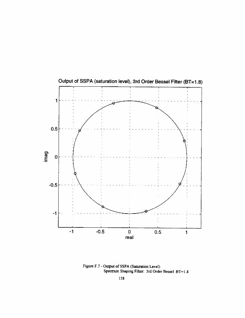
GIE
om
0.5
0
-0.5
-1
Output of SSPA (saturation level), 3rd Order Bessel Filter (BT=1.8I i i I i
I I I
-1 -0.5 0 0.5real
Figure F.7 - Output of SSPA (Saturation Level)
Spectrum Shaping Filter: 3rd Order Bessel BT= 1.8
158
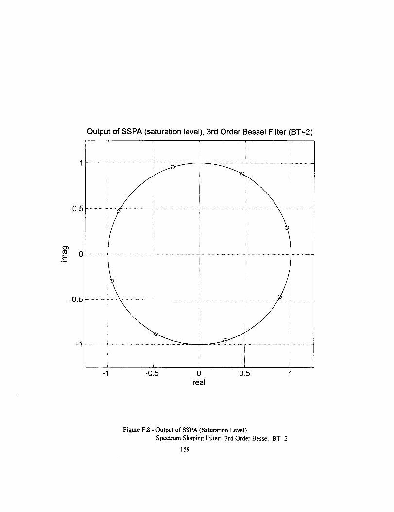
Output of SSPA (saturation level), 3rd Order Bessel Filter (BT=2)
E
0.5
0
-0.5
-1
iiiiiiiiiiiiiiiii iiiiiiiiiiiiiiiiii...................................................................................... i .....................................................................................
1 • .............................iiiiiiiiiiiiiiiiK |
-1 -O.5 0 0.5 1real
Figure F.8 - Output of SSPA (Saturation Level)
Spectrum Shaping Filter: 3rd Order Bessel BT=2
159
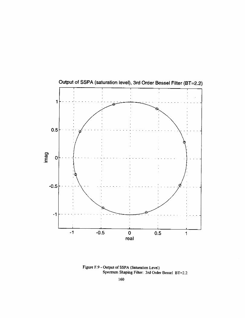
0.5
0
-0.5
-1
Output of SSPA (saturation level), 3rd Order Bessel Filter (BT=2.2)
I 1 I I
-1 -0.5 0 0.5 1real
Figure F.9 - Output of SSPA (Saturation Level)
Speclrum Shaping Filter: 3rd Order Bessel BT=2.2
160
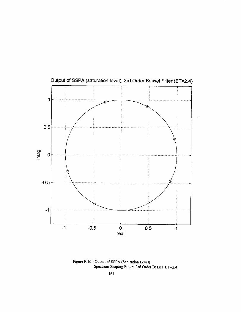
t_E
.m
05
Output of SSPA (saturation level), 3rd Order Bessel Filter (BT=2.4f
................................................. i ............................................................................................................................
o51i ......................i................I
-0.5 0 0.5 1real
Figure F. l 0 - Output of SSPA (Saturation Level)
Spectrum Shaping Filter: 3rd Order Bessel BT=2.4
161
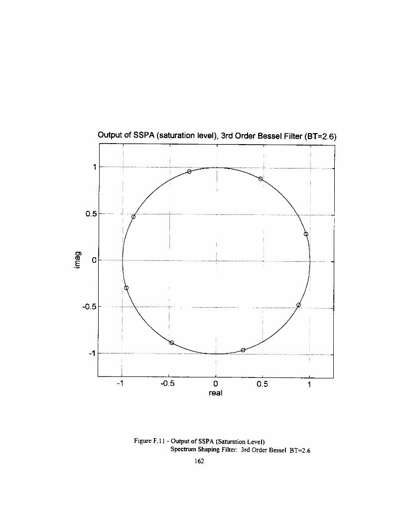
O)
E
Output of SSPA (saturation level), 3rd Order Bessel Filter (BT=2.6
]
1
.................................................... _.................................... _ ................................... , ..................................................
i i
0.5
-0.5
-1
-1 -0.5 0 0.5 1real
Figure F. l I - Output of SSPA (Saturation Level)
Spectrum Shaping Filter: 3rd Order Bessel BT=2.6
162
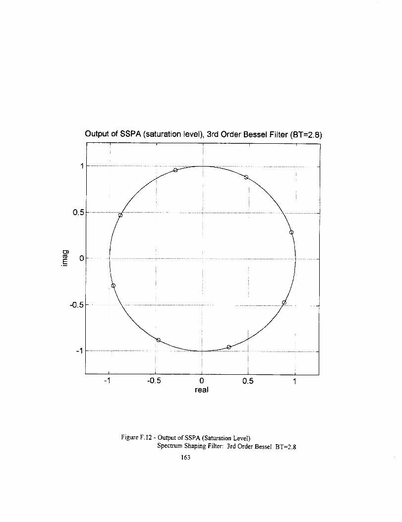
Output of SSPA (saturation level), 3rd Order Bessel Filter (BT=2.8)
E_
E°_
-1 -0.5 0 0.5real
Figure F. 12 - Output of SSPA (Saturation Level)
Speclrum Shaping Filter: 3rd Order Bessel BT=2.8
163

Output of SSPA (saturation level), 3rd Order Bessel Filter (BT=3)
E°_
0.5
0
-0.5
-1
! I I I
..... . ...... _ _ _ .
I I
-1 -0.5 0 0.5 1real
Figure F. 13- Output of SSPA (Saturation Level)
Spectrum Shaping Filter: 3rd Order Bessel BT=3
164
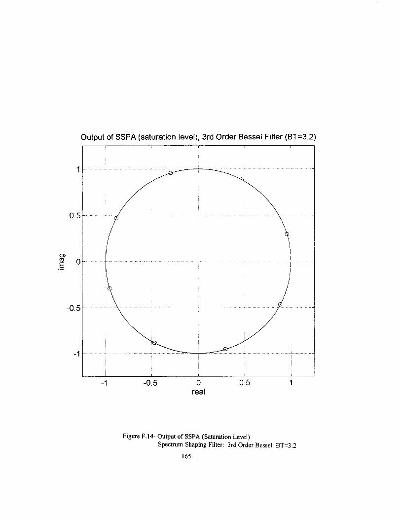
Output of SSPA (saturation level), 3rd Order Bessel Filter (BT=3.2)
E
0.5
0
-0.5
-1
A
I l
-O.5 0 0.5 1real
Figure F. 14- Output of SSPA (Saturation Level)
Spectrum Shaping Filter: 3rd Order Bessel BT=3.2
165
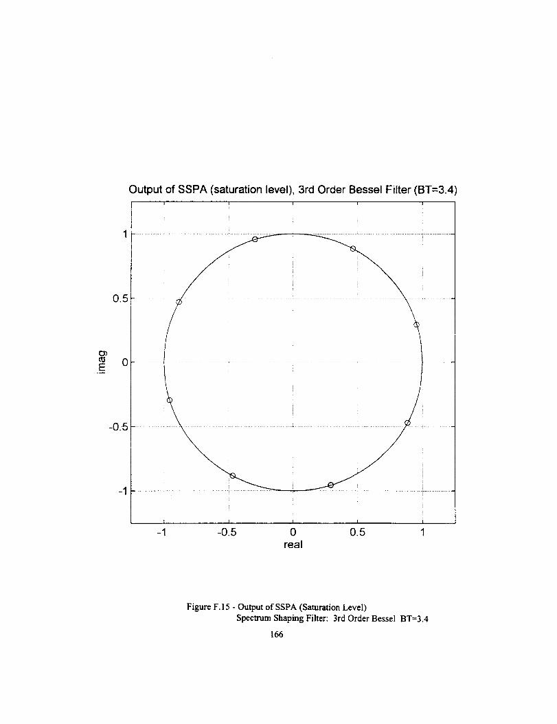
E°_
0.5
0
-0.5
-1
Output of SSPA (saturation level), 3rd Order Bessel Filter (BT=3.4! I I I i
.... i
• !
I I I
-1 -0.5 0 0.5 1real
Figure F. 15 - Output of SSPA (Saturation Level)
Spectrum Shaping Filter: 3rd Order Bessel BT=3.4
166
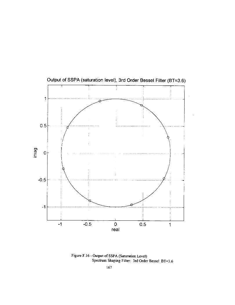
Output of SSPA (saturation level), 3rd Order Bessel Filter (BT=3.6
O3
E
-0.5
-1
-1 -0.5 0 0.5 1real
Figure F. 16 - Output of SSPA (Saturation Level)
Spectrum Shaping Filter: 3rd Order Bessel BT=3.6
167
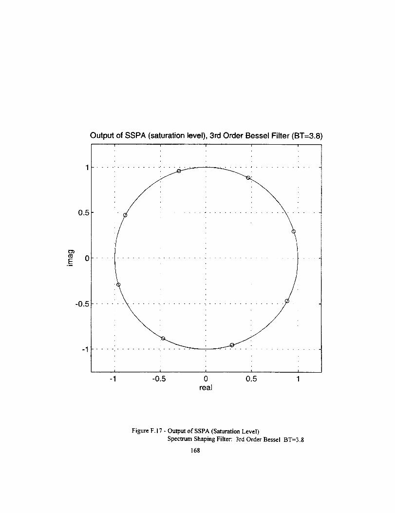
E33
Eo_
0.5
0
-0.5
-1
Output of SSPA (saturation level), 3rd Order Bessel Filter (BT=3.8)I i i I i
| I
-1 -0.5 0 0.5 1
real
Figure F. I ? - Output of SSPA (Saturation Level)
Spectrum Shaping Filter: 3rd Order Bessel BT=3.8
168
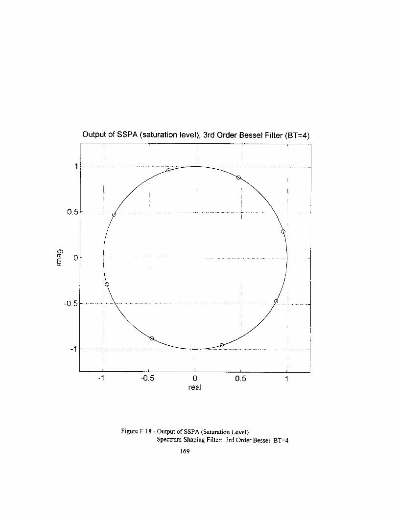
O3
E
Output of SSPA (saturation level), 3rd Order Bessel Filter (BT=4t i _ i
oi . . i
?I I I
-1 43.5 0 0.5 1real
0.5
-0.5
-1
Figure F. 18 - Output of SSPA (Saturation Level)
Spectrum Shaping Filter: 3rd Order Bessel BT=4
169
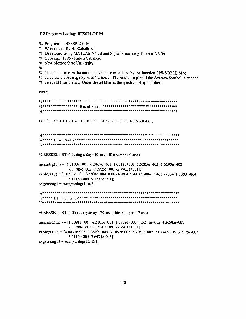
F.2 Program Listing: BESSPLOT.M
% Program : BESSPLOT.M
% Written by : Rub6n Caballero
% Developed using MATLAB V4.2B and Signal Processing Toolbox V3.0b
% Copyright 1996 - Rubgn Caballero
% New Mexico State University%
% This function uses the mean and variance calculated by the function SPWSOBRE.M to
% calculate the Average Symbol Variance. The result is a plot of the Average Symbol Variance
% versus BT for the 3rd Order Bessel filter as the spectrum shaping filter.
clear;
BT=[I 1.05 1.1 1.2 1.4 1.6 1.8 2 2.2 2.4 2.6 2.8 3 3.2 3.4 3.6 3.8 4.0];
% BESSEL : BT=I (using detay=10, ascii file: sampbesl.asc)
meandeg(1,:) = [1.7100e+001 6.2067e+001 1.0712e+002 1.5205e+002 -1.6290e+002
-1.1789e+002 -7.2926e+001-2.7905e+001];
vardeg(1,:) = [1.0221e-003 8.5808e-004 8.0633e-004 9.4189e-004 7.8621e-004 8.2393e-004
8.1116e-004 9.1752e-004];
avgvardegl = sum(vardeg(1,:)yS;
% BESSEL : BT=I.05 (using delay =20, ascii file: sampbesl3.a,c)
meandeg(13,:) = [1.7098e+001 6.2105e+001 1.0709e+002 1.5211e+002-1.6290e+002
-1.1790e+002 -7.2897e+001-2.7901e+001];
vardeg(13,:) = [4.0437e-005 3.3809e-005 3.1692e-005 3.7052e-005 3.0734e-005 3.2129e-0053.2110e-005 3.6434e-005];
avgvardegl3 = sum(vardeg(13,:))/8;
170
% BESSEL : BT=I.1 (using delay =19, ascii file: sampbes8.asc)
meandeg(8,:) = [1.7098e+00t 6.2101e+001 1.0710e+002 1.5210e+002-1.6290e+002
-1.1790e+002 -7.2900e+001 -2.7902e+001];vardeg(8,:) = [9.9913e-006 8.3489e-006 7.8251e-006 9.1203e-006 7.5720e-006 7.9193e-006
7.9803e-006 9.0411e-006];avgvardeg8 = sum(vardeg(8,:))/8;
% BESSEL : BT=I.2 (using delay =17, ascii file: sampbes4.asc)
meandeg(4,:) = [1.7099e+001 6.2083e+001 1.0711e+002 1.5208e+002-1.6290e+002
-I.1790e+002-7.2914e+001-2.7903e+001];
vardeg(4,:) = [2.4972e-004 2.0951e-004 1.9659e-004 2.3032e-004 1.9168e-004 2.0041e-004
1.9809e-004 2.2399e-004];avgvardeg4= sum(vardeg(4,:))/8;
% BESSEL • BT=I.4 (using delay = 24, ascii file: sampbes5.asc)
meandeg(5,:) = [1.7101e+001 6.2102e+001 1.0710e+002 1.5210e+002-1.6290e+002
-1.1790e+002-7.2899e+001-2.7899e+001];vardeg(5,:) = [1.3749e-006 1.1572e-006 1.1217e-006 1.2701e-006 1.1957e-006 1.2262e-006
1.1256e-006 1.2264e-006];avgvardeg5 = sum(vardeg(5,:))/8;
% BESSEL : BT=1.6 (using delay = 22, ascii file: sampbes6.asc)
meandeg(6,:) = [ 1.7106e+001 6.2104e+001 1.0711 e+002 1.5210e+002 - 1.6289e+002
- 1.1789e+002 -7.2896e+001 -2.7894e+001 ];vardeg(6,:) = [4.5746e-006 3.8329e-006 3.5877e-006 4.2036e-006 3.3338e-006 3.5724e-006
3.6400e-006 4.1172e-006];
avgvardeg6 = sum(vardeg(6,:))/8;
171
%BESSEL"BT=I.8(usingdelay= 29, ascii file: sampbes7.asc)
meandeg(7,:) = [1.7109e+001 6.2107e+001 1.0711e+002 1.5211e+002 -1.6289e+002
-1.1789e+002 -7.2892e+001-2.7891e+001];vardeg(7,:) = [1.6004e-006 1.3463e-006 1.2807e-006 1.4545e-006 1.1838e-006 1.2862e-006
1.3147e-006 1.4452e-006];avgvardeg7 = sum(vardeg(7,:))/8;
% BESSEL • BT=2 (using delay = 17, ascii file: sampbes2.asc)
meandeg(2,:) = [1.7109e+001 6.2109e+001 1.071 le+O02 1.521 le+002 -1.6289e+002
- 1.1789e+002 -7.2891 e+O01 -2.7891 e+001 ];
vardeg(2,:) = [4.4990e-008 3.8308e-008 5.1507e-008 5.3124e-008 5.0042e-008 5.9081 e-008
6.3786e-008 4.0034e-008];
avgvardeg2 = sum(vardeg(2,:))/8;
% BESSEL • BT=2.2 (using delay = 31, ascii file: sampbes9.asc)
meandeg(9,:) =[ 1.7108e+001 6.2106e+001 1.0711 e+002 1.5211 e+002 - 1.6289e+002 - 1.1789e+002
-7.2893e+001 -2.7893e+001 ];vardeg(9,:) = [1.0595e-006 8.9530e-007 8.6564e-007 9.7955e-007 9.1845e-007 9.8303e-007
8.653 le-007 9.4939e-007];avgvardeg9 = sum(vardeg(9,:))/8;
% BESSEL : BT=2.4 (using delay = 29, ascii file: sambesl0.asc)
meandeg(10,:) = [1.7105e+001 6.2104e+001 1.0711e+002 1.5210e+002-1.6290e+002
-1.1790e+002 -7.2896e+001-2.7895e+001];
vardeg(10,:) = [5.5214e-007 4.6563e-007 4.7792e-007 5.3915e-007 5.5696e-007 5.8688e-007
4.5275e-007 4.8757e-007];
avgvardegl0 = sum(vardeg(10,:))/8;
172
%BESSEL•BT=2.6(usingdelay=27,asciifile:sambesll.asc)
meandeg(il,:)= [1.7101e+0016.2100e+0011.0710e+0021.5210e+002-1.6290e+002-I.1790e+002-7.2899e+001-2.7899e+001];
vardeg(ll,:)= [4.0654e-0073.4041e-0073.8516e-0074.1756e-0074.7282e-0074.7462e-0073.4439e-0073.5223e-007];
avgvardegll= sum(vardeg(ll,:))/8;
%BESSEL•BT=2.8(usingdelay=25,asciifile:sambesl2.asc)
meandeg(12,:)= [1.7096e+0016.2095e+0011.0710e+0021.5209e+002-1.6290e+002-1.1790e+002-7.2904e+001-2.7904e+001];
vardeg(12,:)=[4.5417e-0073.8038e-0074.5201e-0074.5872e-0075.5238e-0075.1875e-0074.0865e-0073.9254e-007];
avgvardegl2= sum(vardeg(12,:))/8;
%BESSEL-BT=3(usingdelay=40,asciifile:sampbes3.asc)
meandeg(3,:)= [1.7092e+0016.2092e+0011.0709e+0021.5209e+002-1.6291e+002-1.1791e+002-7.2908e+001-2.7908e+001];
vardeg(3,:)= [5.8291e-0083.9094e-0081.2009e-0071.2832e-0071.0620e-0071.1197e-0077.1450e-0083.9674e-008];
avgvardeg3=sum(vardeg(3,:))/8;
%BESSEL"BT=3.2(usingdelay=28,asciifile:sambesl4.asc)
meandeg(14,:)= [1.7088e+00!6.2088e+0011.0709e+0021.5209e+002-1.6291e+002-1.1791e+002-7.2911e+001-2.7912e+001];
vardeg(14,:)= [5.4259e-0083.5312e-0081.4483e-0071.0340e-0071.1655e-0078.1064e-008!.3418e-0074.1300e-008];
avgvardegl4=sum(vardeg(14,:))/8;
173
% BESSEL : BT=3.4 (using delay = 28, ascii file: sarnbesl 5.asc)
meandeg(15,:) = [1.7084e+001 6.2084e+001 1.0708e+002 1.5208e+002-1.6292e+002
- 1.1792e+002 -7.2915e+O01 -2.7916e+001 ];
vardeg(15,:)=[4.0005e-008 2.5838e-008 1.4176e-007 7.8527e-008 1.1756e-007 6.8254e-008
1.472 le-007 2.9590e-008];
avgvardeg 15 = sum(vardeg(15,:))/8;
% BESSEL : BT=3.6 (using delay = 28, ascii file: sambesl6.asc)
meandeg(16,:) = [1.7081e+001 6.2081e+001 1.0708e+002 1.5208e+002-1.6292e+002
-1.1792e+002-7.2919e+O01-2.7919e+001];
vardeg(16,:) = [3.1934e-008 2.0872e-008 1.3377e-007 6.1400e-008 1.0893e-007 5.5746e-0081.5336e-007 2.3636e-008];
avgvardegl6 = sum(vardeg(16,:))/8;
% BESSEL : BT=3.8 (using delay = 28, sambesl 7.asc)
meandeg(l 7,:) = [ 1.7078e+001 6.2078e+001 1.0708e+002 !.5208e+002 -1.6292e+002- 1.1792e+002 -7.2921 e+001 -2.7922e+001 ];
vardeg(17,:)= [2.5426e-008 1.6786e-008 1.2010e-007 4.7555e-008 9.4054e-008 4.3259e-008
1.5054e-007 1.9058e-008];
avgvardeg 17 = sum(vardeg(l 7,:))/8;
% BESSEL : BT=4 (using delay = 28, sambesl 8.asc)
meandeg(l 8,:) = [1.7076e+001 6.2075e+001 1.0708e+002 1.5208e+002 - 1.6292e+002
- 1.1792e+002 -7.2924e+001 -2.7924e+001 ];
vardeg(l 8,:) = [1.9867e-008 1.3236e-008 1.0380e-007 3.6088e-008 7.805 le-008 3.2460e-0081.4042e-007 1.5133e-008];
avgvardeg 18 = sum(vardeg(18,:))/8;
174
0//O*********************************** *
%************** PLOTS***************ICI/O* * * * ** 1" * * * 11"** * * 1"**** * 1..1.** * * * *
% Average Variance for the Symbols
figure(I);
whitebg;
AMPMavgvar = [avgvardegl avgvardeg 13 avgvardeg8 avgvardeg4 avgvardeg5 avgvardeg6
avgvardeg7 avgvardeg2 avgvardeg9 avgvardegl0 avgvardeg 11 avgvardeg 12
avgvardeg3 avgvardeg 14 avgvardeg 15 avgvardeg 16 avgvardeg 17 avgvardeg 18];
% interpolation using spline fit
interBTl =1:0.1:4.0;
interpol 1=interp 1(BT,AMPMavgvar, interBT 1,'spline');
plot(BT,AMPMavgvar,'ok',interBT 1,(interpol 1),'k');
plot(BT,AMPMavgvar,'ok');
title('3rd Order Bessel Filter Symbol Average Variance vs BT');xlabel('Bandwidth-Time Product (BT)');
ylabel(' Variance in Degrees');
grid;
175
APPENDIX G
SCATTER PLOTS:
SRRC FILTER
This appendix contains the Scatter Plots of the output of the SSPA when a Square Root Raised
Cosine (SRRC) Filter is used after the 8PSK Modulator. The Scatter Plots were produced for a=0.1 to
l using the SPWSOBRE.M function. Also, the listing of the program SRRCPLOT.M written in
Matlab which was used to produce the Average Symbol Variance plot (see Figure 3.47 in this report)
is included. All the values of mean and variance in this program were calculated in the program
SPWSOBRE.M.
G.I Scatter Plots
176
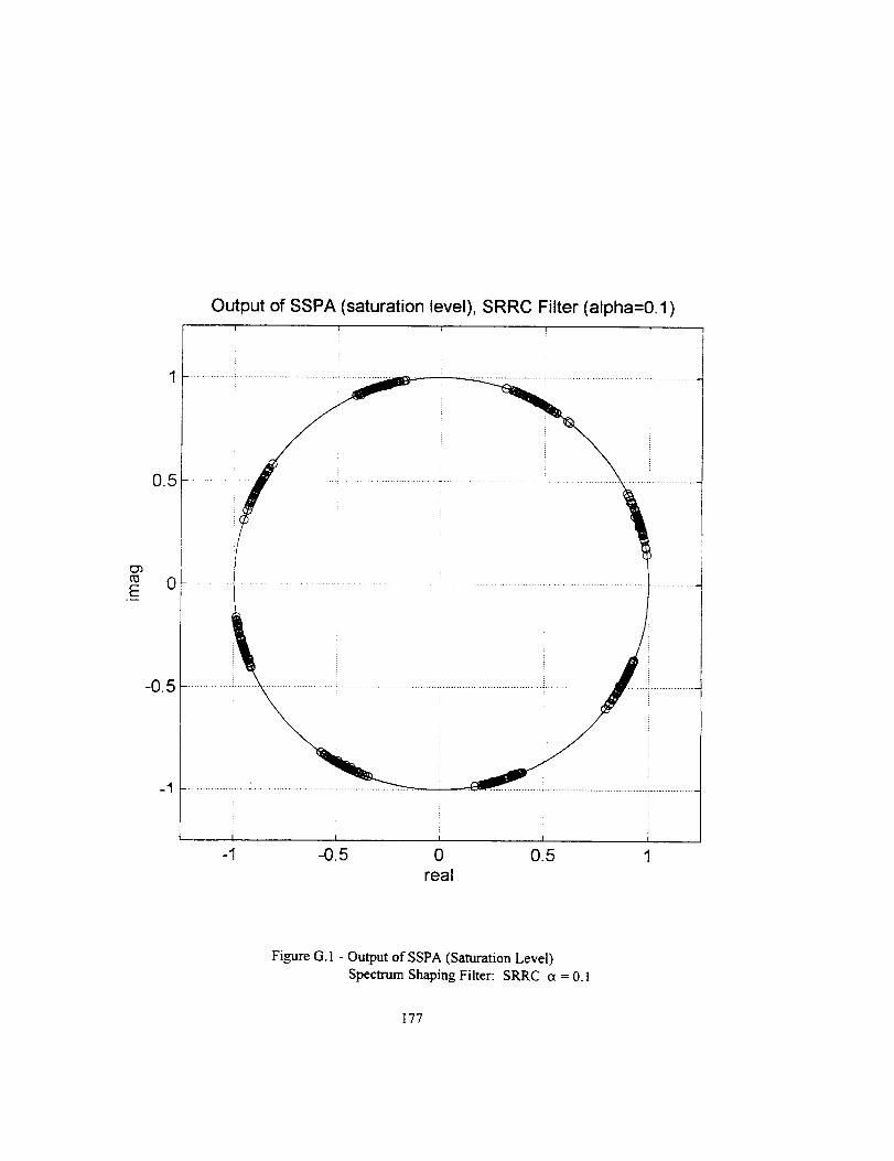
O3
E
0.5
0
-0.5
-1
Output of SSPA (saturation level), SRRC Filter (alpha=0.1)I I t ! I
- ...... . ...........
ii i i i
-1 -0.5 0 0.5
real
Figure G. 1 - Output of SSPA (Saturation Level)
Spectrum Shaping Filter: SRRC ct = O. ]
177
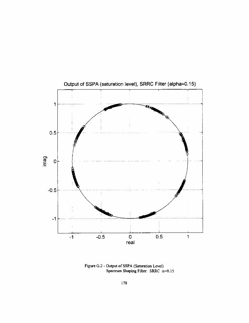
Output of SSPA (saturation level), SRRC Filter (alpha=0.15)
E
0.5
0
-0.5
-1
! i ! i i
-1 -0.5 0 0.5 1real
Figure G.2 - Output of SSPA (Saturation Level)
Spectrum Shaping Filter: SRRC ct=0.15
178
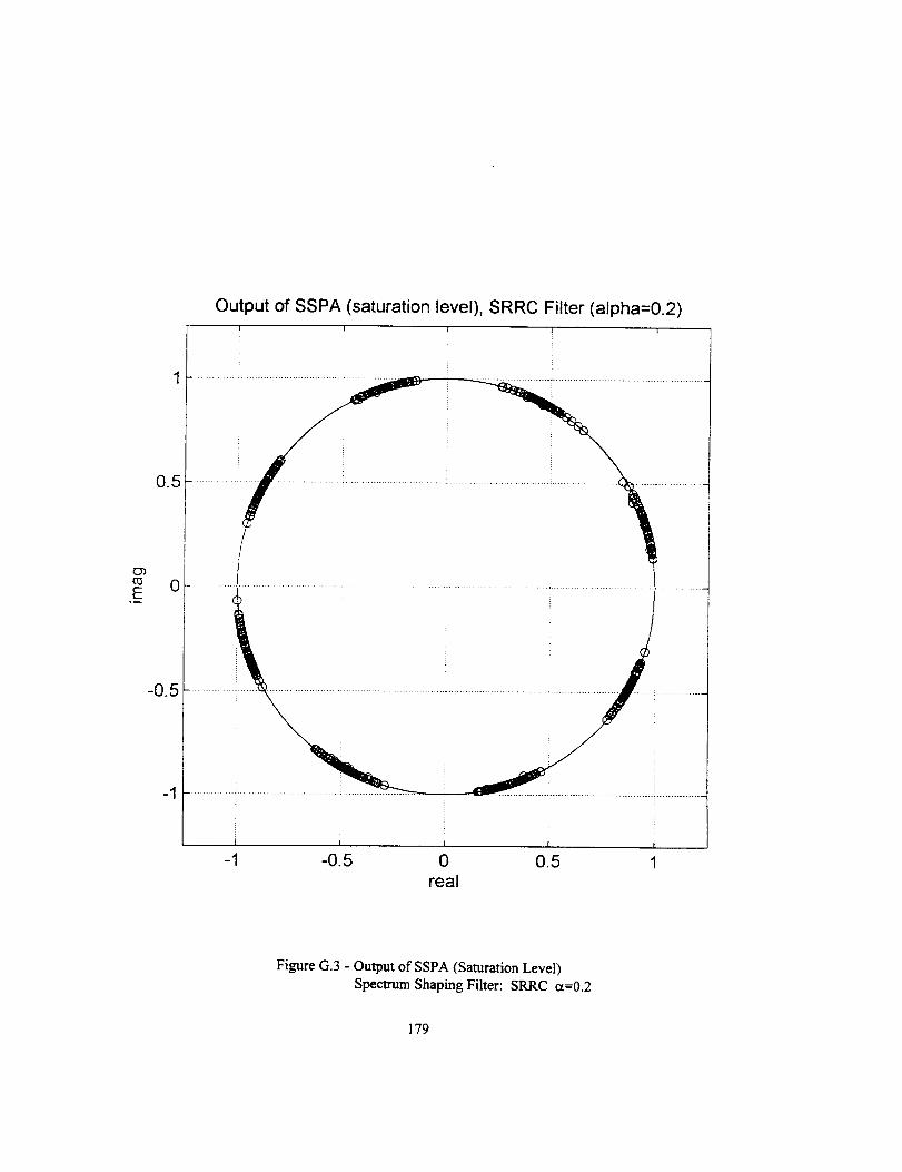
Output of SSPA (saturation level), SRRC Filter (alpha=0.2)
0.5
r
-0.5 ............... - ................
l I I i
-1 -0.5 0 0.5 1real
Figure G.3 - Output of SSPA (Saturation Level)
Spectrum Shaping Filter: SRRC ct=0.2
179
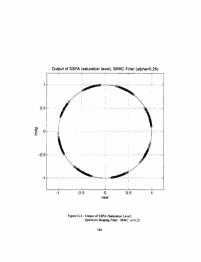
E°u
Output of SSPA (saturation level), SRRC Filter (alpha=0.25)
i i !
1 !i0.5
-0.5
-1
...............................................................................................................................
ii iiiiiiiiI I i I I
-1 -0.5 0 0.5 1real
Figure G.4 - Output of SSPA (Saturation Level)
Spectrum Shaping Filter: SRRC ct=0.25
180
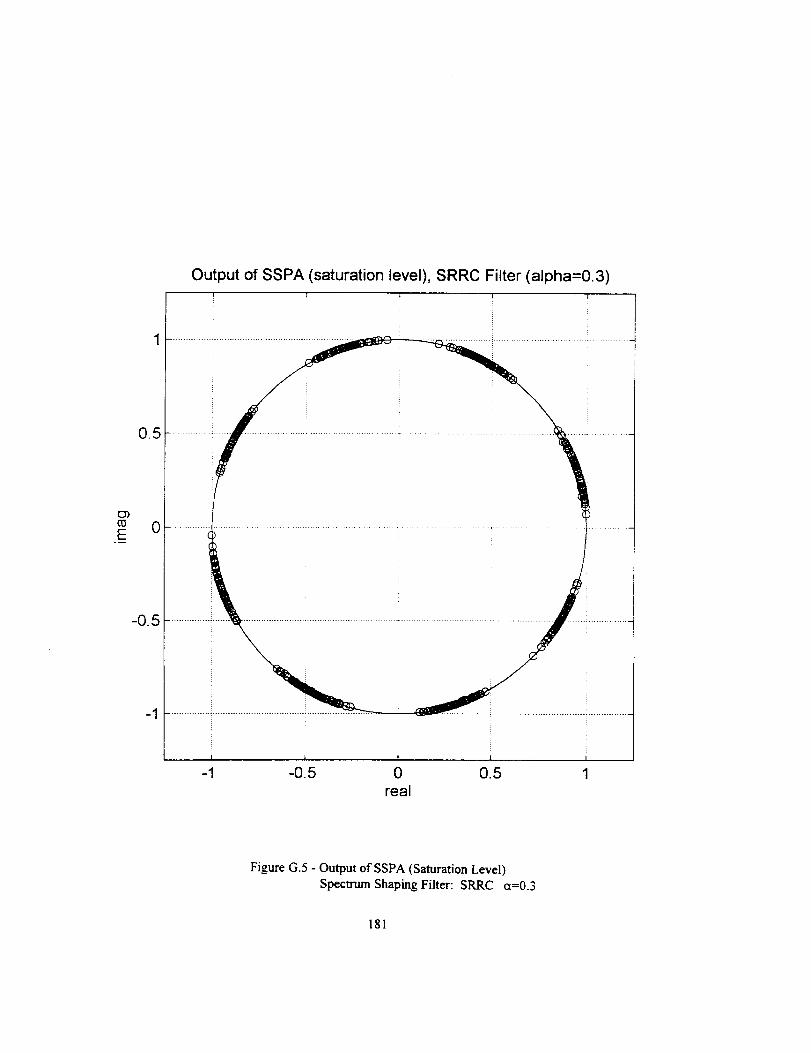
Output of SSPA (saturation level), SRRC Filter (alpha=0.3)
E
0.5
0
-0.5
-1
I J I I
-1 -0.5 0 0.5 1
real
Figure G.5 - Output of SSPA (Saturation Level)
Spectrum Shaping Filter: SRRC a=0.3
181
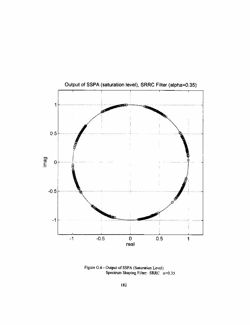
Output of SSPA (saturation level), SRRC Filter (alpha=0.35)I I
E
0.5
-0.5
-1
-1 -0.5 0 0.5
real
Figure G.6 - Output of SSPA (Saturation Level)
Spectrum Shaping Filter: SRRC a=0.35
182
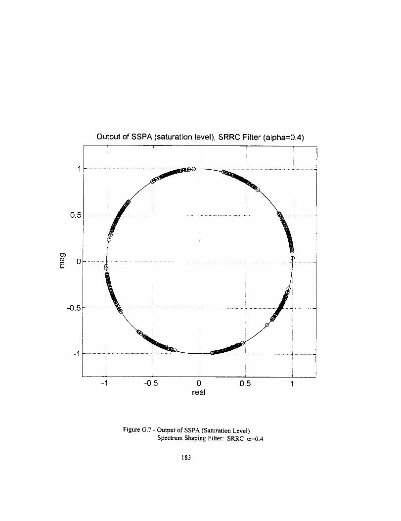
Output of SSPA (saturation level), SRRC Filter (alpha=0.4)
O3
E°n
0.5
0
-0.5
-1
-1 -0.5 0 0.5 1real
Figure G.7 - Output of SSPA (Saturation Level)
Spectrum Shaping Filter: SRRC ct=0.4
183
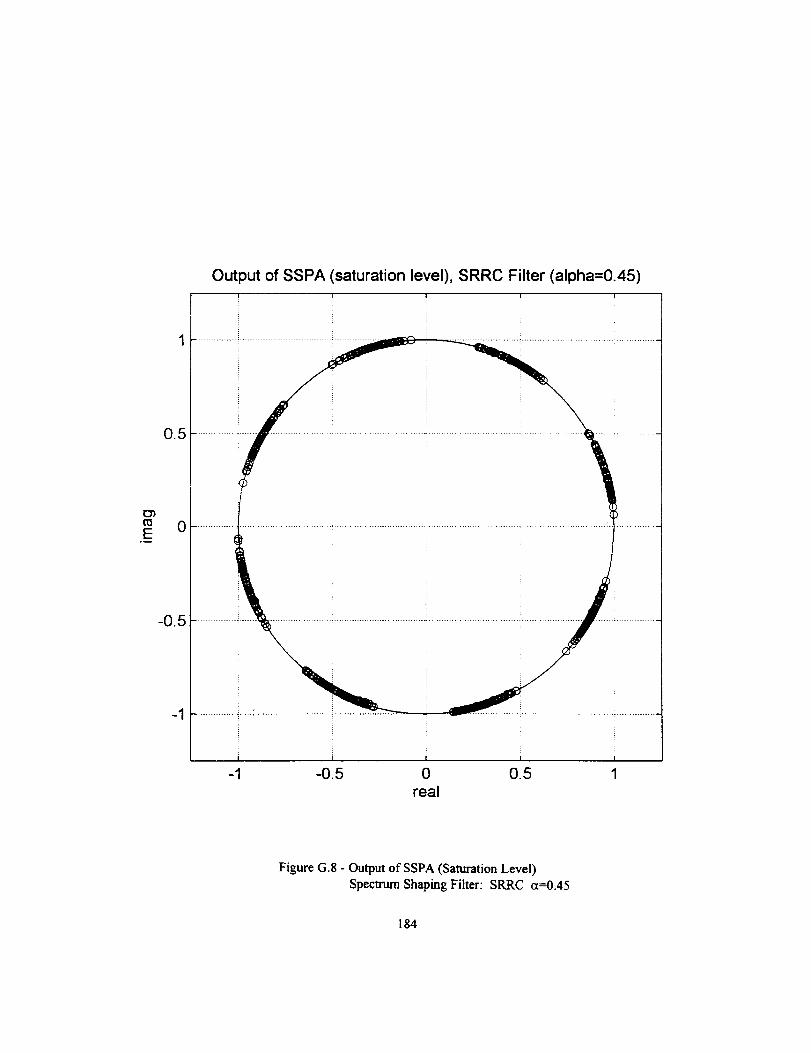
E°_
0.5
0
-0.5
-1
Out )ut of SSPA (saturation level), SRRC Filter (alpha=0.45)I ] t i
i
i
I I i I I
-1 -O.5 0 O.5 1real
Figure G.8 - Output of SSPA (Saturation Level)
Spectrum Shaping Filter: SRRC a=0.45
184
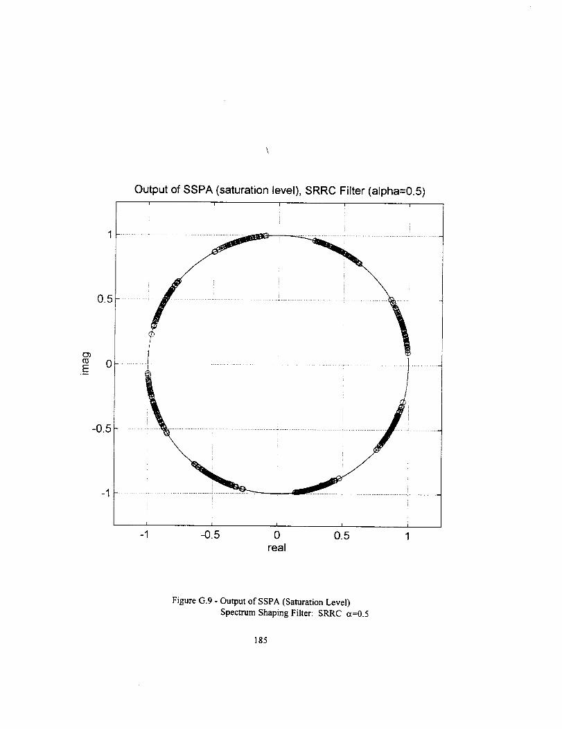
Output of SSPA (saturation level), SRRC Filter (alpha=0.5)I 1 I I
-1 -0.5 0 0.5
real
Figure G.9 - Output of SSPA (Saturation Level)
Spectrum Shaping Filter: SRRC ct=0.5
185
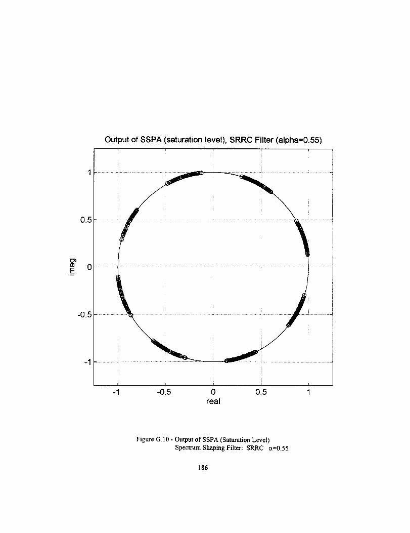
Output of SSPA (saturation level), SRRC Filter (alpha=0.55)
E_¢g
E
1¸¸¸¸! i i05
.............................................................................................................................................
1 i |
-1 -0.5 0 0.5 1
real
Figure G. ] 0 - Output of SSPA (Saturation Level)
Spectrum Shaping Filter: SRRC a=0.55
186
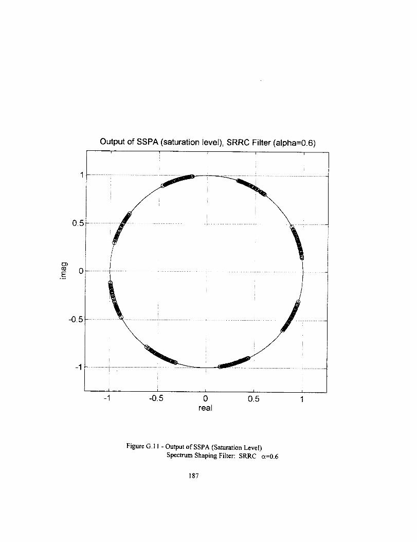
Output of SSPA (saturation level), SRRC Filter (alpha=0.6)
-1 -0.5 0 0.5
real
Figure G. 11 - Output of SSPA (Saturation Level)
Spectrum Shaping Filter: SRRC ct=0.6
187
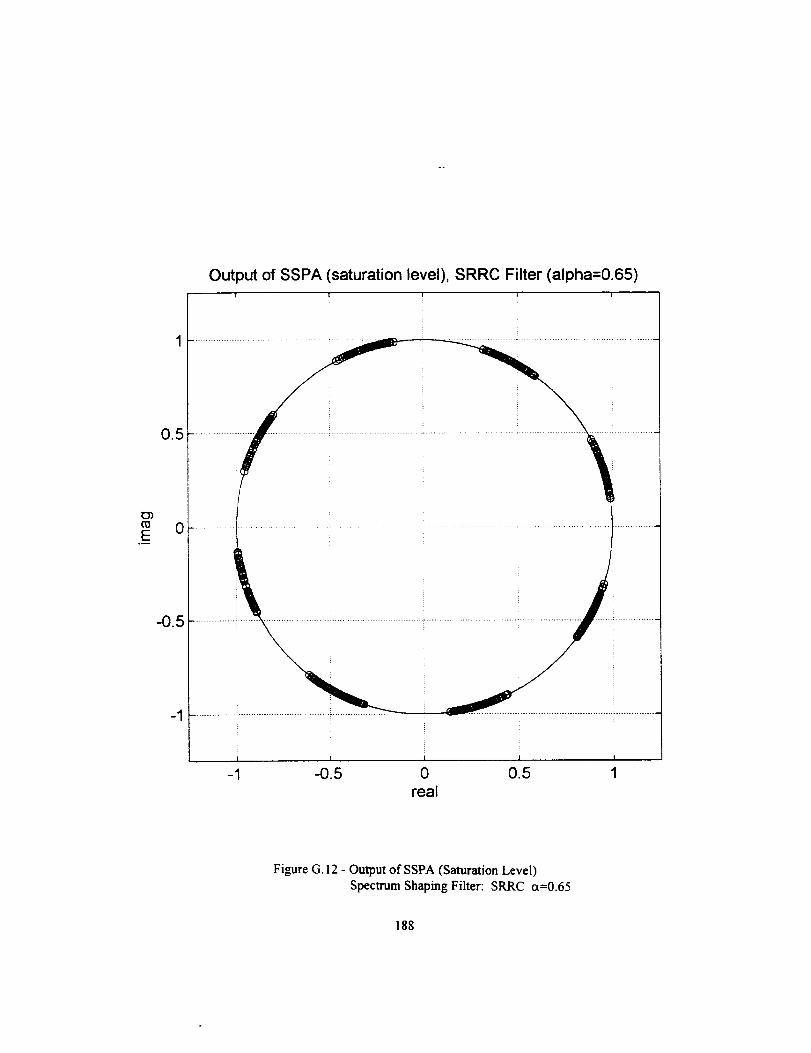
Output of SSPA saturation level), SRRC Filter (alpha=0.65)
11 ii0.5
I _ 1 I
-1 -O.5 0 0.5 1
real
Figure G. 12 - Output of SSPA (Saturation Level)
Spectrum Shaping Filter: SRRC ct=0.65
188
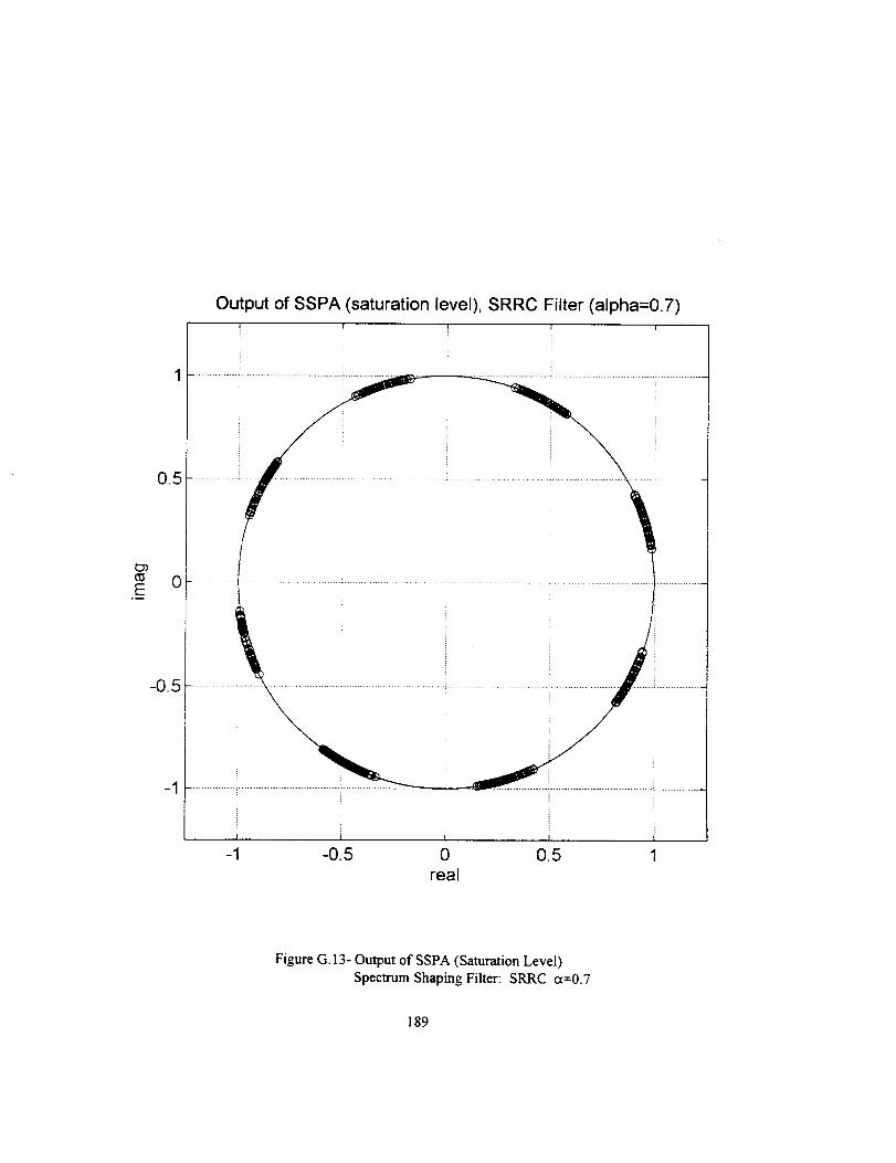
Output of SSPA (saturation level), SRRC Filter (alpha=0.7)
E°__
0.5
0
-0.5
-1
! I !
t i 1
-1 -0.5 0 0.5 1real
Figure G. 13- Output of SSPA (Saturation Level)
Spectrum Shaping Filter: SRRC a=0.7
189
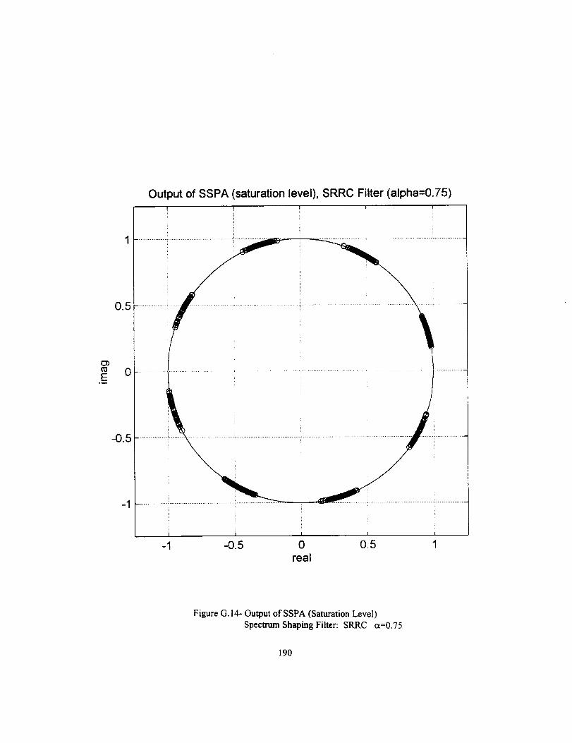
or)
E.w
0.5
0
-0.5
-1
Oul _ut of SSPA (saturation level), SRRC Filter (alpha=0.75)
-O.5 0 O.5 1real
Figure G. 14- Output of SSPA (Saturation Level)
Spectnun Shaping Filter: SRRC a=0.75
190
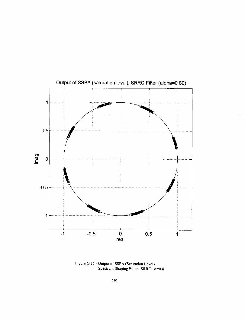
Output of SSPA (saturation level), SRRC Filter (alpha=0.80)
o)
E
0.5
0
-0.5
-1
-1 -0.5 0 0.5 1real
Figure G.I 5 - Output of SSPA (Saturation Level)
Spectrum Shaping Filter: SRRC cc=0.8
191
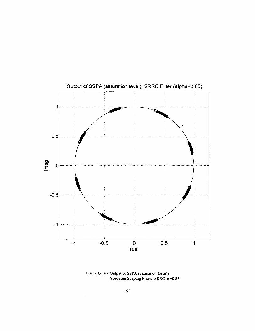
Output of SSPA (saturation level), SRRC Filter (alpha=0.85)
O)
E._
0.5
-0.5
-1
...........................................................................................
i l i i i
-1 -0.5 0 0.5 1
real
Figure G. 16 - Output of SSPA (Saturation Level)
Spectrum Shaping Filter: SRRC a--0.85
192
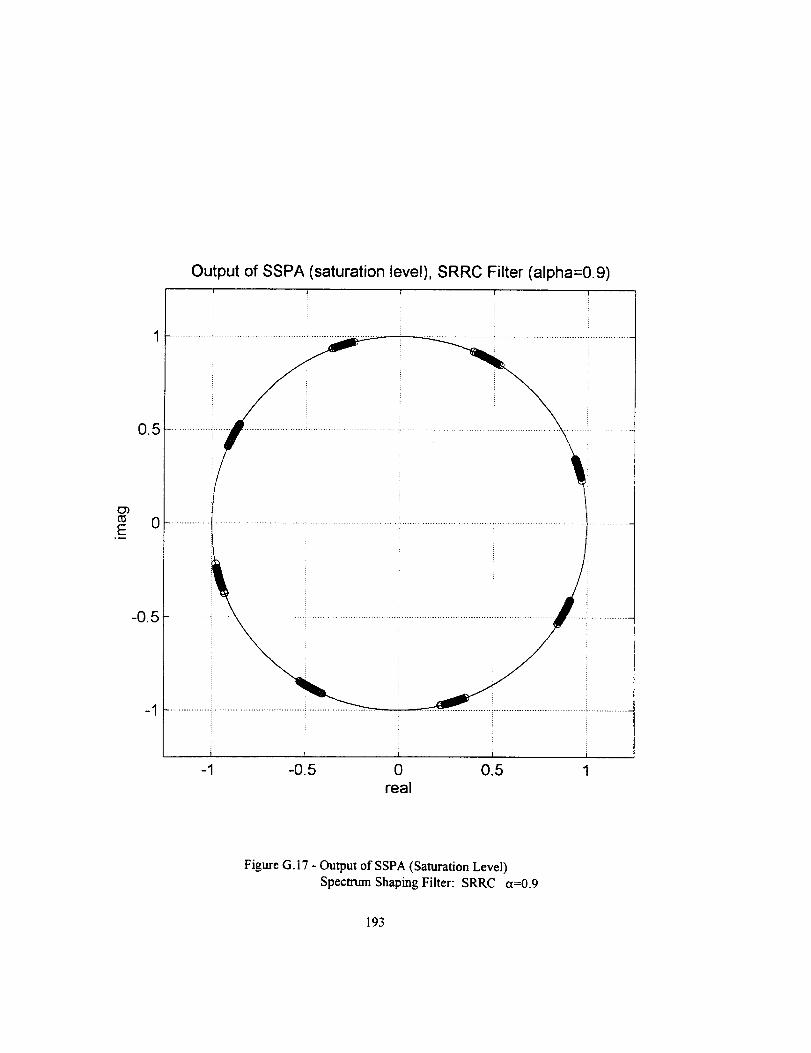
E
05
Output of SSPA saturation level), SRRC Filter (alpha=0.9)
i"...............................................................................................................................................
oI........................iI I I
-1 -0.5 0 0.5 1real
Figure G. 17 - Output of SSPA (Saturation Level)
Spectrum Shaping Filter: SRRC a=0.9
193
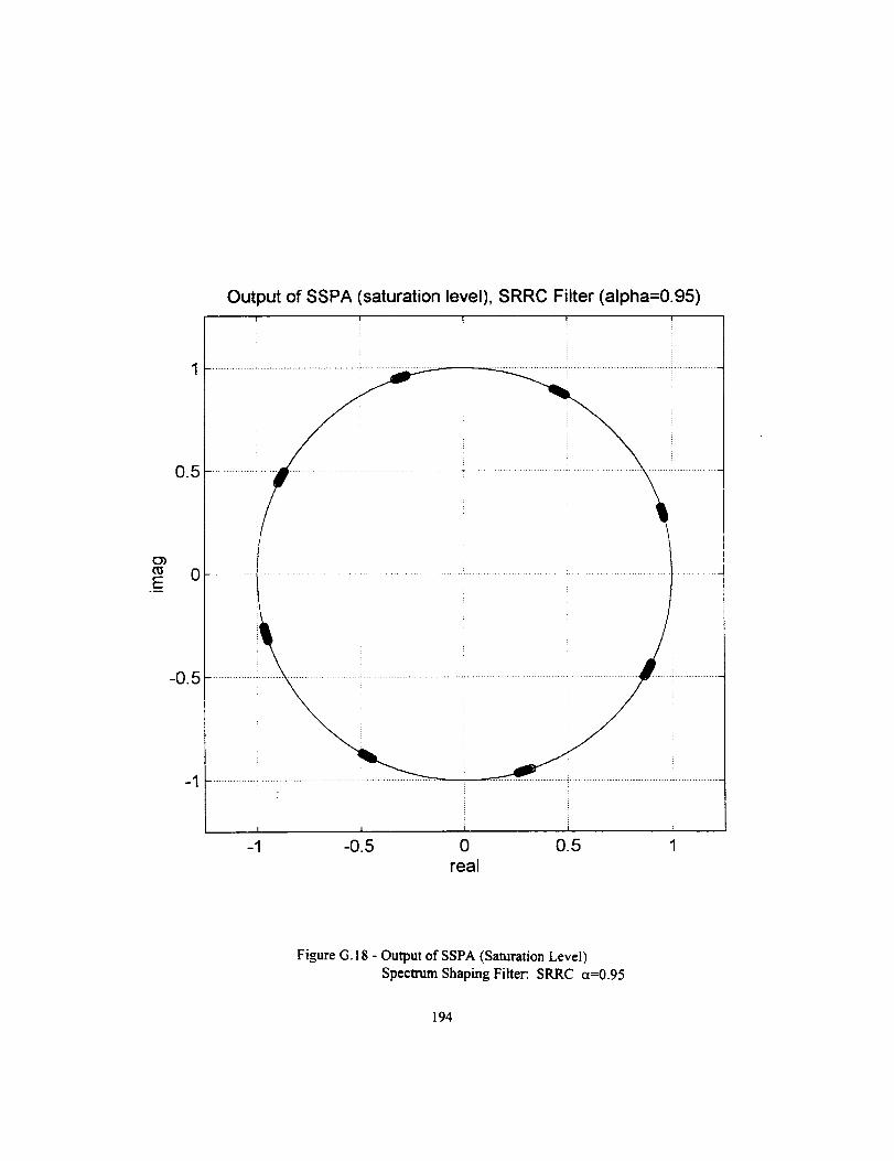
E.m
0.5
Output of SSPA (saturation level), SRRC Filter (alpha=0.95)
! ! ! J
i"............................................................................................
-1
i , I t
-1 -0.5 0 0.5real
Figure G. 18 - Output of SSPA (Saturation Level)
Spectrum Shaping Filter: SRRC ct=0.95
194
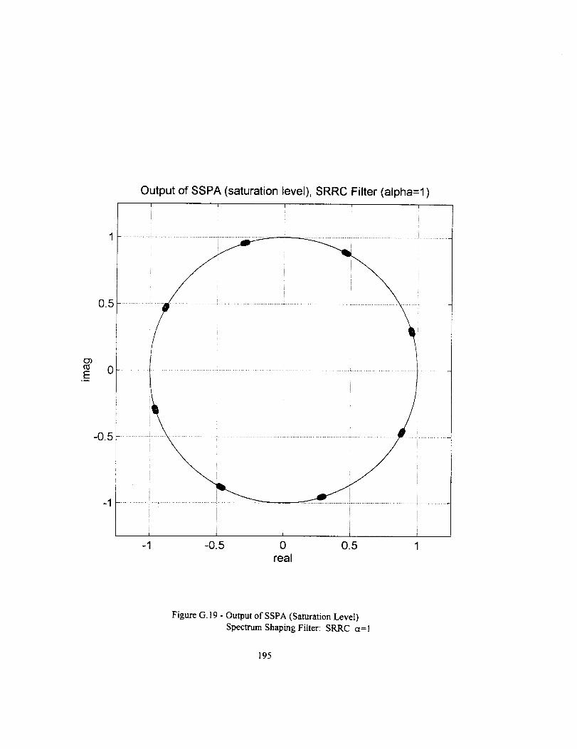
O3
E
0.5
-0.5
-1
Output of SSPA (saturation level), SRRC Filter (alpha=l)i J
i
.................................................... .......................... _ .......................................
i , , i T
-1 -0.5 0 0.5 1real
Figure G. 19 - Output of SSPA (Saturation Level)
Spectrum Shaping Filter: SRRC ct=l
195
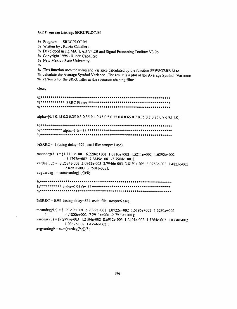
G.2 Program Listing: SRRCPLOT.M
% Program : SRRCPLOT.M
% Written by : Rub6n Caballero
% Developed using MATLAB V4.2B and Signal Processing Toolbox V3.0b% Copyright 1996 - Rub6n Caballero
% New Mexico State University%
% This function uses the mean and variance calculated by the function SPWSOBRE.M to
% calculate the Average Symbol Variance. The result is a plot of the Average Symbol Variance% versus ct for the SRRC filter as the spectrum shaping filter.
clear;
%SRRC = 1 (using delay--521, ascii file: samprcl.asc)
meandeg(1,:) = [1.7111e+001 6.2204e+001 1.0710e+002 1.5211e+002-1.6292e+002
-1.1793e+002 -7.2849e+001-2.7908e+001];vardeg(1,:) = [3.2534e-003 3.0962e-003 3.7946e-003 3.8191e-003 3.0762e-003 3.4823e-003
2.8293e-003 3.7601e-003];avgvardegl = sum(vardeg(l,:))/8;
%SRRC = 0.95 (using delay=52 I, ascii file: samprc6.asc)
meandeg(9,:) = [1.7127e+001 6.2099e+001 1.0722e+002 1.5195e+002 -1.6292e+002
-1.1800e+002 -7.2911e+001-2.7973e+001];
vardeg(9,:) = [9.2975e-003 1.2104e-002 8.6912e-003 1.2401e-002 1.5264e-002 1.0330e-002
1.0367e-002 !.4794e-002];
avgvardeg9 = sum(vardeg(9,:))/8;
196
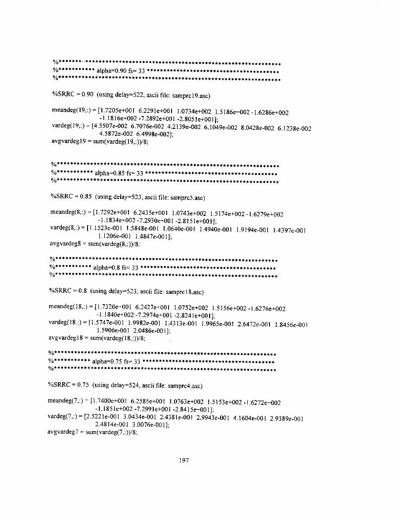
%SRRC= 0.90(usingdelay=522,asciifile:samprcl9.asc)
meandeg(19,:)= [1.7205e+0016.2291e+0011.0734e+0021.5186e+002-1.6286e+002-1.1816e+002-7.2892e+001-2.8051e+001];
vardeg(19,:)=_.5507e-0026.7076e-0024.2139e-0026.1049e-0028.0428e-0026.1238e-0024.5872e-0026.4998e-002];
avgvardegl9=sum(vardeg(19,:))/8;
%SRRC=0.85(usingdelay=523,asciifile:samprc5.asc)
meandeg(8,:)= [1.7292e+0016.2435e+0011.0743e+0021.5174e+002-1.6279e+002-1.1834e+002-7.2930e+001-2.8151e+001];
vardeg(8,:)=[1.1523e-0011.5848e-0011.0640e-0011.4940e-0011.9194e-0011.4397e-0011.1206e-0011.4847e-001];
avgvardeg8= sum(vardeg(8,:))/8;
%SRRC=0.8(usingdelay=523,asciifile:samprcl8.asc)
meandeg(18,:)= [1.7320e+00!6.2427e+0011.0752e+0021.5156e+002-1,6276e+002-1.1840e+002-7.2974e+001-2.8241e+001];
vardeg(18,:)= [1.5747e-0011.9982e-0011.4313e-0011.9965e-0012.6472e-0011.8456e-0011.5906e-0012.0486e-001];
avgvardegl8= sum(vardeg(18,:))/8;
%SRRC=0.75(usingdelay=524,asciifile:samprc4.asc)
meandeg(7,:)=[1.7400e+0016.2585e+0011.0763e+0021.5153e+002-1.6272e+002-1.1851e+002-7.2991e+001-2.8415e+001];
vardeg(7,:)=[2.5221e-00|3.0434e-0012.4381e-0012.9943e-0014.1604e-0012.9389e-0012.4814e-0013.0076e-001];
avgvardeg7= sum(vardeg(7,:))/8;
197
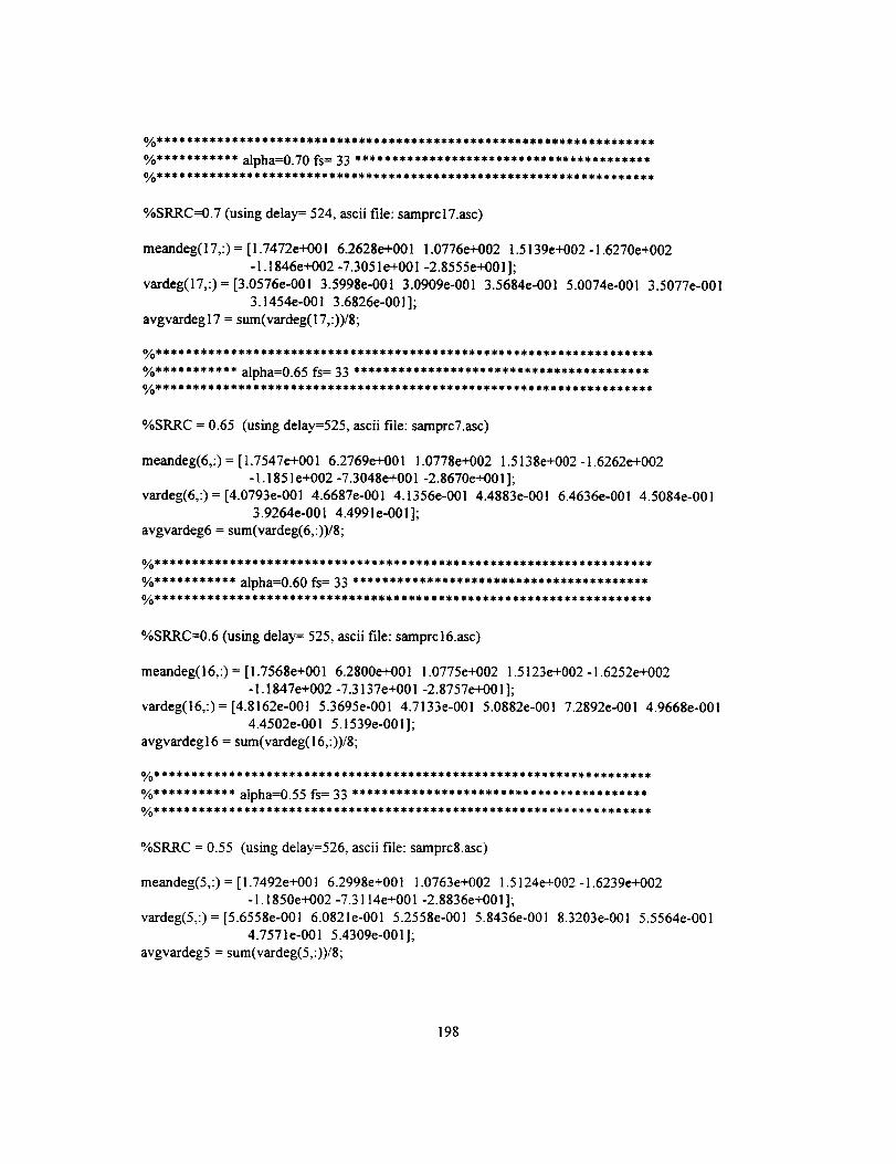
%SRRC=0.7(usingdelay= 524,asciifile: samprcl 7.asc)
meandeg(17,:) = [ 1.7472e+001 6.2628e+001 1.0776e+002 1.5139e+002 - 1.6270e+002
- 1.1846e+002 -7.3051 e+001 -2.8555 e+001 ];
vardeg(17,:)= [3.0576e-001 3.5998e-001 3.0909e-001 3.5684e-001 5.0074e-001 3.5077e-001
3.1454e-001 3.6826e-001];
avgvardeg 17 = sum(vardeg(l 7,:))/8;
%SRRC = 0.65 (using delay=525, ascii file: samprc7.asc)
meandeg(6,:) = [1.7547e+001 6.2769e+001 1.0778e+002 1.5138e+002-1.6262e+002
-1.1851e+002-7.3048e+001 -2.8670e+001];
vardeg(6,:) = [4.0793e-001 4.6687e-001 4.1356e-001 4.4883e-001 6.4636e-001 4.5084e-001
3.9264e-001 4.4991e-001];
avgvardeg6 = sum(vardeg(6,:)ffS;
%SRRC=0.6 (using delay= 525, ascii file: samprcl 6.asc)
meandeg(16,:) = [1.7568e+001 6.2800e+001 1.0775e+002 1.5123e+002-1.6252e+002
-1.1847e+002 -7.3137e+001-2.8757e+001];vardeg(16,:) = [4.8162e-001 5.3695e-001 4.7133e-001 5.0882e-001 7.2892e-001 4.9668e-001
4.4502e-001 5.1539e-001];
avgvardegl6 = sum(vardeg(16,:))/8;
%SRRC = 0.55 (using delay=526, ascii file: samprc8.asc)
meandeg(5,:) = [ 1.7492e+001 6.2998e+001 1.0763e+002 1.5124e+002 - 1.6239e+002
- 1.1850e+002 -7.3114e+001 -2.8836e+001 ];
vardeg(5,:)= [5.6558e-001 6.0821e-001 5.2558e-001 5.8436e-001 8.3203e-001 5.5564e-001
4.7571e-001 5.4309e-001 ];
avgvardeg5 = sum(vardeg(5,:))/8;
198
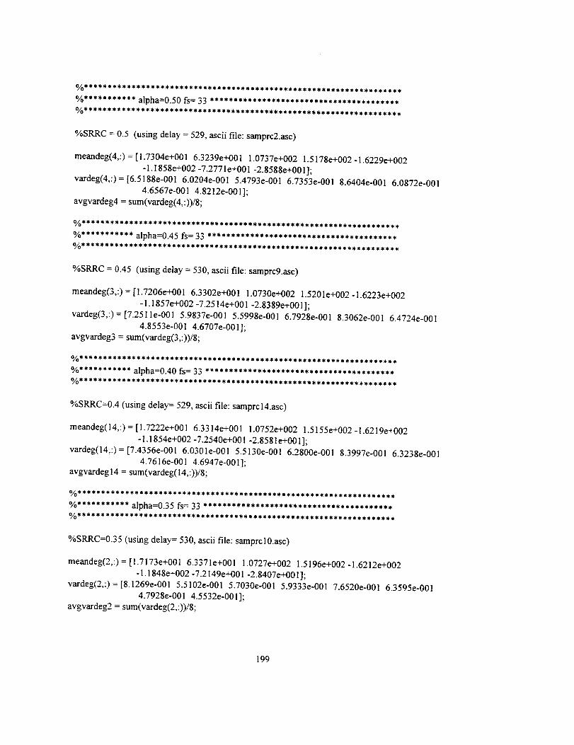
%SRRC= 0.5 (using delay = 529, ascii file: samprc2.asc)
meandeg(4,:) = [ 1.7304e+001 6.3239e+001 1.0737e+002 1.5178e+002 - 1.6229e+002
- 1.1858e+002 -7.2771 e+001 -2.8588e+001 ];
vardeg(4,:)= [6.5188e-001 6.0204e-001 5.4793e-00! 6.7353e-001 8.6404e-001 6.0872e-001
4.6567e-001 4.8212e-001];
avgvardeg4 = sum(vardeg(4,:))/8;
%SRRC = 0.45 (using delay = 530, ascii file: samprc9.asc)
meandeg(3,:) = [1.7206e+001 6.3302e+001 1.0730e+002 1.5201e+002-1.6223e+002
-1.1857e+002 -7.2514e+001-2.8389e+001];
vardeg(3,:) = [7.2511e-001 5.9837e-001 5.5998e-001 6.7928e-001 8.3062e-001 6.4724e-001
4.8553e-001 4.6707e-001];
avgvardeg3 = sum(vardeg(3,:))/g;
%SRRC=0.4 (using delay = 529, ascii file: samprc 14.asc)
meandeg(14,:) = [1.7222e+001 6.3314e+001 1.0752e+002 1.5155e+002 -1.6219e+002
-1.1854e+002 -7.2540e+001-2.8551e+001];
vardeg(14,:) = [7.4356e-001 6.0301e-001 5.5130e-001 6.2800e-001 8.3997e-001 6.3238e-001
4.7616e-001 4.6947e-001];avgvardegl4 = sum(vardeg(14,:))/8;
%SRRC=0.35 (using delay = 530, ascii file: samprcl0.asc)
meandeg(2,:) = [1.7173e+001 6.3371e+001 1.0727e+002 1.5196e+002-1.6212e+002
-1.1848e+002 -7.2149e+001-2.8407e+001];
vardeg(2,:) = [8.1269e-001 5.5102e-001 5.7030e-001 5.9333e-001 7.6520e-001 6.3595e-001
4.7928e-001 4.5532e-001];
avgvardeg2 = sum(vardeg(2,:)_8;
199
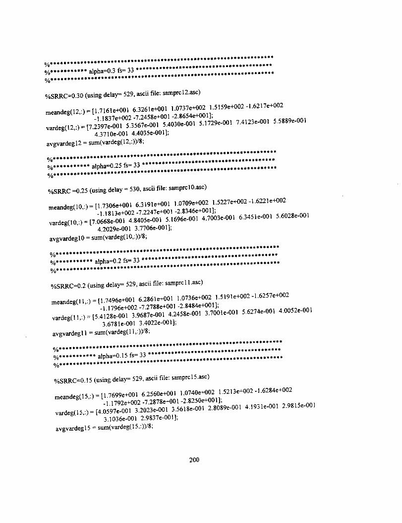
%SRRC=0.30 (using delay = 529, ascii file: samprc 12.asc)
meandeg(12,:) = [1.7161e+001 6.3261e+001 1.0737e+002 1.5159e+002-1.6217e+002
- 1.1837e+002 -7.245ge+001 -2.8654e+001 ];
vardeg(12,:)=[7.2397e-001 5.3567e-001 5.4030e-001 5.1729e-001 7.4123e-001 5.5889e-001
4.3710e-001 4.4035e-001];
avgvardegl2 = sum(vardeg(12,:))/8;
%SRRC =0.25 (using delay = 530, ascii file: samprcl 0.asc)
meandeg(10,:) = [1.7306e+001 6.3191e+001 1.0709e+002 1.5227e+O02-1.622]e+002
-1.1813e+002 -7.2247e+001-2.8346e+00I];
vardeg(10,:) = [7.0668e-001 4.8405e-001 5.1696e-001 4.7003e-001 6.3451e-001 5.6028e-001
4.2029e-001 3.7706e-001];
avgvardegl0 = sum(vardeg(10,:))/8;
%SRRC=0.2 (using delay= 529, ascii file: samprcl l.asc)
meandeg(ll,:)=[1.7496e+001 6.2861e+001 1.0736e+002 1.5191e+002-1.6257e+002
- 1.1796e+002 -7.2788e+001 -2.8484e+001 ];
vardeg(ll,:)= [5.4128e-001 3.9687e-001 4.2458e-001 3.7001e-001 5.6274e-001 4.0052e-001
3.6781e-001 3.4022e-001];
avgvardeg I 1 = sum(vardeg(l I,:))/8;
%SRRC--0.15 (using delay= 529, ascii file: samprcl 5.asc)
meandeg(15,:) = [1.7699e+001 6.2560e+001 1.0740e+002 1.5213e+002 -1.6284e+002
- 1.1792e+002 -7.2878e+001 -2.8250e+001 ];
vardeg(15,:)=[4.0597e-001 3.2023e-001 3.5618e-001 2.8089e-001 4.1931e-001 2.9815e-001
3.1036e-001 2.9837e-001 ];
avgvardeg 15 = sum(vardeg( 15,:))/8;
200
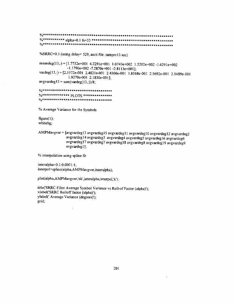
%SRRC=0.1(usingdelay=529,asciifile: samprcl3.asc)
meandeg(13,:) = [1.7752e+001 6.2291e+001 1.0743e+002 1.5202e+002-1.6291e+002
-1.1790e+002 -7.2870e+001-2.8113e+001];
vardeg(13,:) = [2.5572e-001 2.4821e-001 2.4306e-001 1.8168e-001 2.5692e-001 2.0489e-001
1.9270e-001 2.1830e-001];
avgvardegl3 = sum(vardeg(13,:))/8;
% Average Variance for the Symbols
figure(l);
whitebg;
AMPMavgvar= [avgvardegl3 avgvardegl5 avgvardegll avgvardegl0 avgvardegl2 avgvardeg2
avgvardegl4 avgvardeg3 avgvardeg4avgvardeg5 avgvardegl6 avgvardeg6
avgvardegl7 avgvardeg7 avgvardegl8 avgvardeg8 avgvardegl9 avgvardeg9
avgvardegl];
% interpolation using spline fit
interaipha=0.1:0.0001 : 1;
interpol=spline(alpha,AMPMavgvar, interalpha);
plot(alpha,AMPMavgvar,'ok',interaipha,interpol,'k');
title('SRRC Filter Average Symbol Variance vs Roll-of Factor (alpha)');
xlabel('SRRC Rolloff factor (alpha)');
ylabel(' Average Variance (degrees)');
grid;
201


![1 Constant Envelope Signaling in MIMO Channels · arXiv:1605.03779v1 [cs.IT] 12 May 2016 1 Constant Envelope Signaling in MIMO Channels Borzoo Rassouli and Bruno Clerckx Abstract](https://img.pdfslide.us/doc/110x75/5f0322117e708231d407b393/1-constant-envelope-signaling-in-mimo-channels-arxiv160503779v1-csit-12-may.jpg)