1

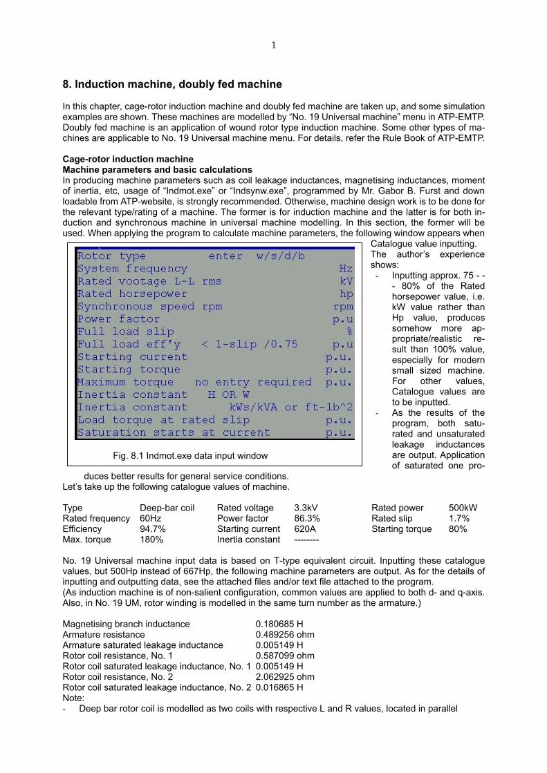
8. Induction machine, doubly fed machine In this chapter, cage-rotor induction machine and doubly fed machine are taken up, and some simulation examples are shown. These machines are modelled by “No. 19 Universal machine” menu in ATP-EMTP. Doubly fed machine is an application of wound rotor type induction machine. Some other types of ma-chines are applicable to No. 19 Universal machine menu. For details, refer the Rule Book of ATP-EMTP. Cage-rotor induction machine Machine parameters and basic calculations In producing machine parameters such as coil leakage inductances, magnetising inductances, moment of inertia, etc, usage of “Indmot.exe” or “Indsynw.exe”, programmed by Mr. Gabor B. Furst and down loadable from ATP-website, is strongly recommended. Otherwise, machine design work is to be done for the relevant type/rating of a machine. The former is for induction machine and the latter is for both in-duction and synchronous machine in universal machine modelling. In this section, the former will be used. When applying the program to calculate machine parameters, the following window appears when

Catalogue value inputting. The author’s experience shows:

- Inputting approx. 75 - - - 80% of the Rated horsepower value, i.e. kW value rather than Hp value, produces somehow more ap-propriate/realistic re-sult than 100% value, especially for modern small sized machine. For other values, Catalogue values are to be inputted.

- As the results of the program, both satu-rated and unsaturated leakage inductances are output. Application of saturated one pro-

duces better results for general service conditions. Let’s take up the following catalogue values of machine. Type Deep-bar coil Rated voltage 3.3kV Rated power 500kW Rated frequency 60Hz Power factor 86.3% Rated slip 1.7% Efficiency 94.7% Starting current 620A Starting torque 80% Max. torque 180% Inertia constant -------- No. 19 Universal machine input data is based on T-type equivalent circuit. Inputting these catalogue values, but 500Hp instead of 667Hp, the following machine parameters are output. As for the details of inputting and outputting data, see the attached files and/or text file attached to the program. (As induction machine is of non-salient configuration, common values are applied to both d- and q-axis. Also, in No. 19 UM, rotor winding is modelled in the same turn number as the armature.) Magnetising branch inductance 0.180685 H Armature resistance 0.489256 ohm Armature saturated leakage inductance 0.005149 H Rotor coil resistance, No. 1 0.587099 ohm Rotor coil saturated leakage inductance, No. 1 0.005149 H Rotor coil resistance, No. 2 2.062925 ohm Rotor coil saturated leakage inductance, No. 2 0.016865 H Note: - Deep bar rotor coil is modelled as two coils with respective L and R values, located in parallel

Fig. 8.1 Indmot.exe data input window

2

- If test/measured values are available, the values are most preferably to be applied. - For magnetising branch, saturation characteristic is applicable in No. 19 program, if necessary. For

leakage inductance saturation, if necessary, TACS/MODELS controlled additional inductances are to be connected outside of the model.

Also the Indmot.exe program produces PCH file, the format of which is directly applicable to EMTP calculation. Using the PCH file, the machine’s starting was calculated. For detail of the program data, see the attached file.

Note: - In the attached data file, spe-

cial initialising technique is ap-plied, which is applicable also for multi-machine case. Detail will be explained later.

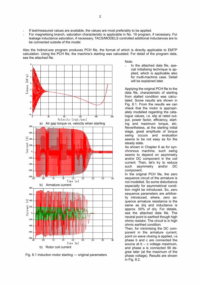
Applying the original PCH file to the data file, characteristic of starting from stalled condition was calcu-lated. Some results are shown in Fig. 8.1. From the results we can check that the motor is appropri-ately modelled regarding the cata-logue values, i.e. slip at rated out-put, power factor, efficiency, start-ing and maximum torque, etc. Nevertheless, at the starting initial stage, great amplitude of torque swing occurs and evaluation seems to be not easy as for the steady state. As shown in Chapter 6 as for syn-chronous machine, such swing seems to depend on asymmetry and/or DC component in the coil current. Then, let’s try to reduce such asymmetry and/or DC component. In the original PCH file, the zero sequence circuit of the armature is not modelled. So some disturbance especially for asymmetrical condi-tion might be introduced. So, zero sequence parameters are arbitrar-ily introduced, where, zero se-quence armature resistance is the same as d/q and inductance is approx. 50% of d/q. For details, see the attached data file. The neutral point is earthed though high ohmic resistor. The circuit is in high ohmic earthed condition. Then, for minimising the DC com-ponent in the armature current, point on wave closing is applied, i.e. phase b and c are connected the source at b – c voltage maximum, and phase a is connected 90 de-gree later (at the maximum of the phase voltage). Results are shown in Fig. 8.2.

a) Air gap torque vs. velocity when starting

b) Armature current

b) Rotor coil current

Fig. 8.1 Induction motor starting --- original parameters

3

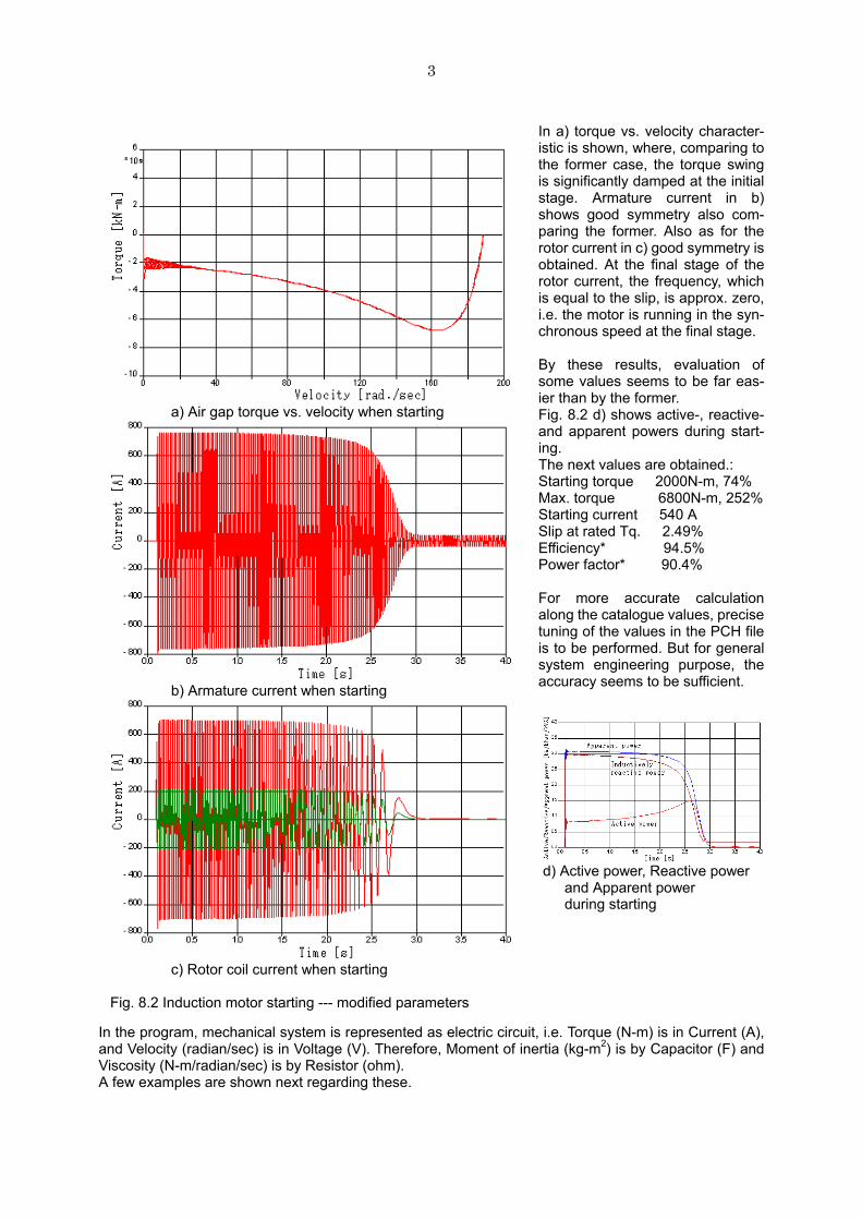
In a) torque vs. velocity character-istic is shown, where, comparing to the former case, the torque swing is significantly damped at the initial stage. Armature current in b) shows good symmetry also com-paring the former. Also as for the rotor current in c) good symmetry is obtained. At the final stage of the rotor current, the frequency, which is equal to the slip, is approx. zero, i.e. the motor is running in the syn-chronous speed at the final stage.

By these results, evaluation of some values seems to be far eas-ier than by the former. Fig. 8.2 d) shows active-, reactive- and apparent powers during start-ing. The next values are obtained.: Starting torque 2000N-m, 74% Max. torque 6800N-m, 252% Starting current 540 A Slip at rated Tq. 2.49% Efficiency* 94.5% Power factor* 90.4% For more accurate calculation along the catalogue values, precise tuning of the values in the PCH file is to be performed. But for general system engineering purpose, the accuracy seems to be sufficient.

In the program, mechanical system is represented as electric circuit, i.e. Torque (N-m) is in Current (A), and Velocity (radian/sec) is in Voltage (V). Therefore, Moment of inertia (kg-m2) is by Capacitor (F) and Viscosity (N-m/radian/sec) is by Resistor (ohm). A few examples are shown next regarding these.

a) Air gap torque vs. velocity when starting

b) Armature current when starting

c) Rotor coil current when starting Fig. 8.2 Induction motor starting --- modified parameters

d) Active power, Reactive power and Apparent power during starting

4

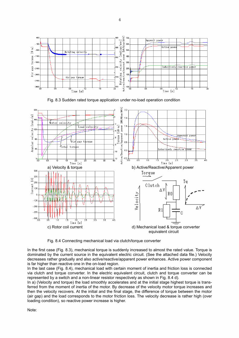
In the first case (Fig. 8.3), mechanical torque is suddenly increased to almost the rated value. Torque is dominated by the current source in the equivalent electric circuit. (See the attached data file.) Velocity decreases rather gradually and also active/reactive/apparent power enhances. Active power component is far higher than reactive one in the on-load region. In the last case (Fig. 8.4), mechanical load with certain moment of inertia and friction loss is connected via clutch and torque converter. In the electric equivalent circuit, clutch and torque converter can be represented by a switch and a non-linear resistor respectively as shown in Fig. 8.4 d). In a) (Velocity and torque) the load smoothly accelerates and at the initial stage highest torque is trans-ferred from the moment of inertia of the motor. By decrease of the velocity motor torque increases and then the velocity recovers. At the initial and the final stage, the difference of torque between the motor (air gap) and the load corresponds to the motor friction loss. The velocity decrease is rather high (over loading condition), so reactive power increase is higher. Note:

Fig. 8.3 Sudden rated torque application under no-load operation condition

a) Velocity & torque b) Active/Reactive/Apparent power

c) Rotor coil current d) Mechanical load & torque converter equivalent circuit

Fig. 8.4 Connecting mechanical load via clutch/torque converter

5

Active/reactive/apparent power is calculated by the next equations.:

22 )(Re)(

3)()()(Re

poweractivepowerActivepowerApparent

IVVIVVIVVpoweractive

IVIVIVpowerActive

cabbcaabc

ccbbaa

+=

−+−+−=

++=

For inductively reactive power, minus value appears by the equation. Multi machine case The restrictions in multi machine case are, : - Uniform initialisation mode is to be applied to any machine in No. 19 universal machine menu. - In initialisation, giving slip to every machine produces most stable result to the author’s experience. - PREDICTION and solidly earthed armature coil neutral are mandatory for multi machine case. - For cases of more than 3 machines (generally), “ABSOLUTE U.M. DIMENSIONS” card is to be ap-

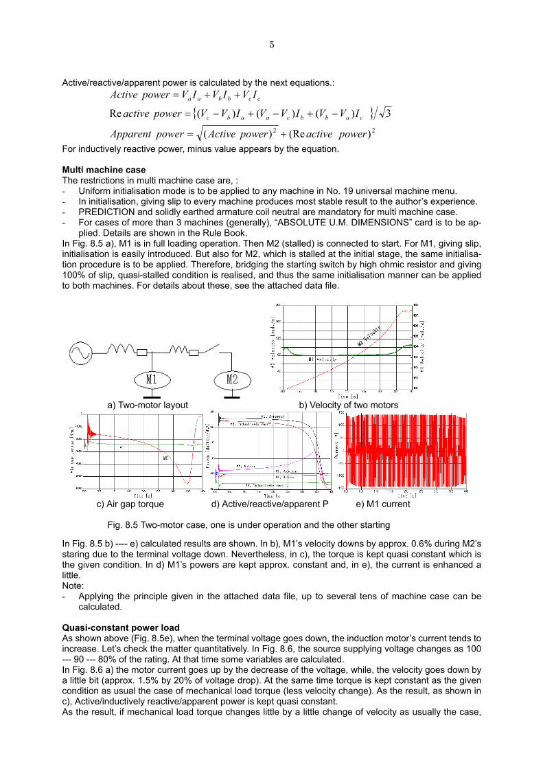
plied. Details are shown in the Rule Book. In Fig. 8.5 a), M1 is in full loading operation. Then M2 (stalled) is connected to start. For M1, giving slip, initialisation is easily introduced. But also for M2, which is stalled at the initial stage, the same initialisa-tion procedure is to be applied. Therefore, bridging the starting switch by high ohmic resistor and giving 100% of slip, quasi-stalled condition is realised, and thus the same initialisation manner can be applied to both machines. For details about these, see the attached data file.

In Fig. 8.5 b) ---- e) calculated results are shown. In b), M1’s velocity downs by approx. 0.6% during M2’s staring due to the terminal voltage down. Nevertheless, in c), the torque is kept quasi constant which is the given condition. In d) M1’s powers are kept approx. constant and, in e), the current is enhanced a little. Note: - Applying the principle given in the attached data file, up to several tens of machine case can be

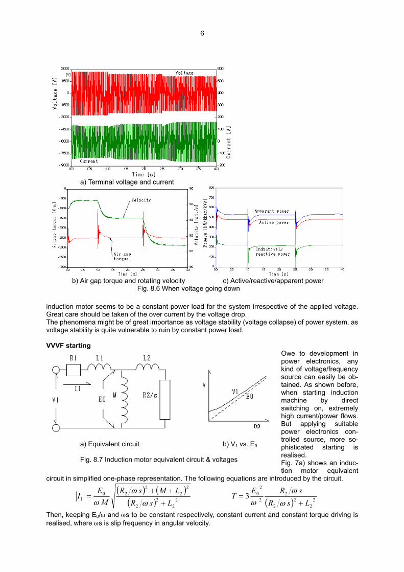
calculated. Quasi-constant power load As shown above (Fig. 8.5e), when the terminal voltage goes down, the induction motor’s current tends to increase. Let’s check the matter quantitatively. In Fig. 8.6, the source supplying voltage changes as 100 --- 90 --- 80% of the rating. At that time some variables are calculated. In Fig. 8.6 a) the motor current goes up by the decrease of the voltage, while, the velocity goes down by a little bit (approx. 1.5% by 20% of voltage drop). At the same time torque is kept constant as the given condition as usual the case of mechanical load torque (less velocity change). As the result, as shown in c), Active/inductively reactive/apparent power is kept quasi constant. As the result, if mechanical load torque changes little by a little change of velocity as usually the case,

a) Two-motor layout b) Velocity of two motors

c) Air gap torque d) Active/reactive/apparent P e) M1 current

Fig. 8.5 Two-motor case, one is under operation and the other starting

6

induction motor seems to be a constant power load for the system irrespective of the applied voltage. Great care should be taken of the over current by the voltage drop. The phenomena might be of great importance as voltage stability (voltage collapse) of power system, as voltage stability is quite vulnerable to ruin by constant power load. VVVF starting

Owe to development in power electronics, any kind of voltage/frequency source can easily be ob-tained. As shown before, when starting induction machine by direct switching on, extremely high current/power flows. But applying suitable power electronics con-trolled source, more so-phisticated starting is realised. Fig. 7a) shows an induc-tion motor equivalent

circuit in simplified one-phase representation. The following equations are introduced by the circuit.

( ) ( )( ) ( ) 2

22

2

22

20

22

22

22

220

1 3LsRsRE

TLsRLMsR

ME

I+

=+

++=

ωω

ωωω

ω

Then, keeping E0/ω and ωs to be constant respectively, constant current and constant torque driving is realised, where ωs is slip frequency in angular velocity.

a) Terminal voltage and current

b) Air gap torque and rotating velocity c) Active/reactive/apparent power

Fig. 8.6 When voltage going down

a) Equivalent circuit b) V1 vs. E0 Fig. 8.7 Induction motor equivalent circuit & voltages

7

So, supplying linearly rising voltage with linearly rising frequency, starting with constant torque, i.e. ac-celeration, and constant current is expected. This is the most simplified VVVF controlling. For more sophisticated controlling, turning of V1 (terminal voltage) as shown in Fig. 8.7 b) is to be applied. In the following example, TACS controlled voltage source is applied, where the voltage wave shape is mathematically created in the TACS. For details, see the attached data file. Actually such voltage source is realised by power electronics circuit, which will be explained in the fol-lowing chapter (chapter 10).

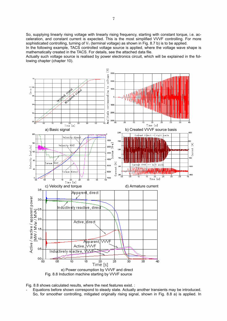
Fig. 8.8 shows calculated results, where the next features exist. : - Equations before shown correspond to steady state. Actually another transients may be introduced.

So, for smoother controlling, mitigated originally rising signal, shown in Fig. 8.8 a) is applied. In

a) Basic signal b) Created VVVF source basis

c) Velocity and torque d) Armature current

e) Power consumption by VVVF and direct Fig. 8.8 Induction machine starting by VVVF source

8

TACS, it is created by time-delaying function (s-block). - The voltage source controlling TACS signal is created (Fig. 8.8 b) ), where both the amplitude and

the frequency are proportional to the signal value. Care should be taken that, if ω in (cos ωt) is not constant (time-varying), the frequency of (cos ωt) is not ω. The time-integration of angular velocity is to be applied to θ in (cos θ). See the attached file.

- The signal is specified to realise the similar starting characteristics as by the direct source connect-ing start before shown. Quasi-constant torque excepting at the initial time interval and linearly rising velocity characteristics are obtained. See Fig. 8.8 c)

- Armature currents between both start method are significantly different, as in Fig. 8.8 d) - Most remarkable difference is in power consumption as shown in Fig. 8.8 e). As for the integration of

the apparent power, the value in VVVF is only approx. 10% of in the direct one. Also as for active power, only approx. 25%.

Doubly fed machine Originally wound rotor type induction machine was used for obtaining higher starting torque. Owing to development in power electronics, such usage has been decreased and higher efficiency of cage-rotor type has been applied as shown before, such as VVVF inverter starting. Today’s main usage of wound-rotor type is application to doubly fed machine as variable speed Motor/Generator in pumping station. Also the usage for flywheel generator is expected. In this section, basic feature/response of doubly fed machine is surveyed.

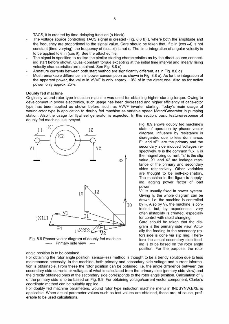
Fig. 8.9 shows doubly fed machine’s state of operation by phasor vector diagram. Influence by resistance is disregarded due to less dominance. E1 and sE1 are the primary and the secondary side induced voltages re-spectively. Φ is the common flux. I0 is the magnetizing current. “s” is the slip value. X1 and X2 are leakage reac-tance of the primary and secondary sides respectively. Other variables are thought to be self-explanatory. The machine in the figure is supply-ing lagging power factor of load power. V1 is usually fixed in power system. Giving I2, the whole diagram can be drawn, i.e. the machine is controlled by I2. Also by V2, the machine is con-trolled, but, by experiences, very often instability is created, especially for control with rapid changing. Care should be taken that the dia-gram is the primary side view. Actu-ally the feeding to the secondary (ro-tor) side is done via slip ring. There-fore the actual secondary side feed-ing is to be based on the rotor angle position. For the purpose, the rotor

angle position is to be obtained. For obtaining the rotor angle position, sensor-less method is thought to be a trendy solution due to less maintenance necessity. In the machine, both primary and secondary side voltage and current informa-tion is obtainable. From these the rotor position can be obtained, i.e. the angle difference between the secondary side currents or voltages of what is calculated from the primary side (primary side view) and the directly obtained ones at the secondary side corresponds to the rotor angle position. Calculation of I2 of the primary side is to be based on Fig. 8.9. For obtaining voltage/current vector component, Clarke’s coordinate method can be suitably applied. For doubly fed machine parameters, wound rotor type induction machine menu in INDSYNW.EXE is applicable. When actual parameter values such as test values are obtained, those are, of cause, pref-erable to be used calculations.

Fig. 8.9 Phasor vector diagram of doubly fed machine ----- Primary side view ----

9

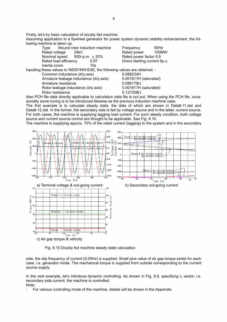
Firstly, let’s try basic calculation of doubly fed machine. Assuming application to a flywheel generator for power system dynamic stability enhancement, the fol-lowing machine is taken up. Type Wound rotor induction machine Frequency 50Hz Rated voltage 24kV Rated power 100MW Nominal speed 500r.p.m. + 20% Rated power factor 0.9 Rated load efficiency 0.97 Direct starting current 5p.u. Inertia const. 10s Inputting these values to INDSYNW.EXE, the following values are obtained. : Common inductance (d/q axis) 0.088234H Armature leakage inductance (d/q axis) 0.001617H (saturated) Armature resistance 0.086179Ω Rotor leakage inductance (d/q axis) 0.001617H (saturated) Rotor resistance 0.127258Ω Also PCH file data directly applicable to calculation data file is out put. When using the PCH file, occa-sionally some tuning is to be introduced likewise as the previous induction machine case. The first example is to calculate steady state, the data of which are shown in Data8-11.dat and Data8-12.dat. In the former, the secondary side is fed by voltage source and in the latter, current source. For both cases, the machine is supplying lagging load current. For such steady condition, both voltage source and current source control are thought to be applicable. See Fig. 8.10. The machine is supplying approx. 70% of the rated current (lagging) to the system and in the secondary

side, the slip frequency of current (0.05Hz) is supplied. Small plus value of air gap torque exists for each case, i.e. generator mode. The mechanical torque is supplied from outside corresponding to the current source supply. In the next example, let’s introduce dynamic controlling. As shown in Fig. 8.9, specifying I2 vector, i.e. secondary side current, the machine is controlled. Note: - For various controlling mode of the machine, details will be shown in the Appendix.

a) Terminal voltage & out-going current b) Secondary out-going current

c) Air gap torque & velocity Fig. 8.10 Doubly fed machine steady state calculation

10

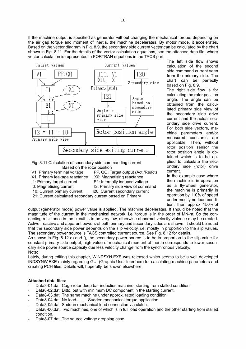
If the machine output is specified as generator without changing the mechanical torque, depending on the air gap torque and moment of inertia, the machine decelerates. By motor mode, it accelerates. Based on the vector diagram in Fig. 8.9, the secondary side current vector can be calculated by the chart shown in Fig. 8.11. For the details of the vector calculation equations, see the attached data file, where vector calculation is represented in FORTRAN equations in the TACS part.

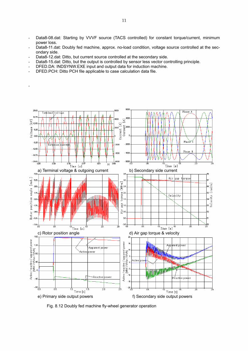
The left side flow shows calculation of the second side command current seen from the primary side. The chart can be perfectly based on Fig. 8.9. The right side flow is for calculating the rotor position angle. The angle can be obtained from the calcu-lated primary side view of the secondary side drive current and the actual sec-ondary side drive current. For both side vectors, ma-chine parameters and/or measured constants are applicable. Then, without rotor position sensor the rotor position angle is ob-tained which is to be ap-plied to calculate the sec-ondary side (rotor) drive current. In the example case where the machine is in operation as a fly-wheel generator, the machine is primarily in operation by 110% of speed under mostly no-load condi-tion. Then, approx. 150% of

output (generator mode) power value is applied. The machine decelerates. It should be noted that the magnitude of the current in the mechanical network, i.e. torque is in the order of MN-m. So the con-necting resistance in the circuit is to be very low, otherwise abnormal velocity violence may be created. Active, reactive and apparent powers of both primary and secondary sides are shown. It should be noted that the secondary side power depends on the slip velocity, i.e. mostly in proportion to the slip values. The secondary power source is TACS controlled current source. See Fig. 8.12 for details. As shown in Fig. 8.12 e) and f), the secondary power source is to be in proportion to the slip value for constant primary side output, high value of mechanical moment of inertia corresponds to lower secon-dary side power source capacity due less velocity change from the synchronous velocity. Note: Lately, during editing this chapter, WINDSYN.EXE was released which seems to be a well developed INDSYNW.EXE mainly regarding GUI (Graphic User Interface) for calculating machine parameters and creating PCH files. Details will, hopefully, be shown elsewhere. Attached data files: - Data8-01.dat: Cage rotor deep bar induction machine, starting from stalled condition. - Data8-02.dat: Ditto, but with minimum DC component in the starting current. - Data8-03.dat: The same machine under approx. rated loading condition. - Data8-04.dat: No load ------- Sudden mechanical torque application. - Data8-05.dat: Sudden mechanical load connection via clutch. - Data8-06.dat: Two machines, one of which is in full load operation and the other starting from stalled

condition. - Data8-07.dat: The source voltage dropping case.

Fig. 8.11 Calculation of secondary side commanding current Based on the rotor position V1: Primary terminal voltage PP, QQ: Target output (Act./React) X1: Primary leakage reactance X0: Magnetising reactance I1: Primary target current E1: Internally induced voltage I0: Magnetising current I2: Primary side view of command I10: Current primary current I20: Current secondary current I21: Current calculated secondary current based on Primary

11

- Data8-08.dat: Starting by VVVF source (TACS controlled) for constant torque/current, minimum power loss.

- Data8-11.dat: Doubly fed machine, approx. no-load condition, voltage source controlled at the sec-ondary side.

- Data8-12.dat: Ditto, but current source controlled at the secondary side. - Data8-15.dat: Ditto, but the output is controlled by sensor less vector controlling principle. - DFED.DA: INDSYNW.EXE input and output data for induction machine. - DFED.PCH: Ditto PCH file applicable to case calculation data file. -

a) Terminal voltage & outgoing current b) Secondary side current

c) Rotor position angle d) Air gap torque & velocity

e) Primary side output powers f) Secondary side output powers Fig. 8.12 Doubly fed machine fly-wheel generator operation

12

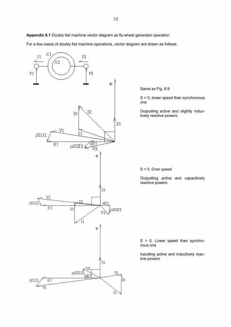
Appendix 8.1 Doubly fed machine vector diagram as fly-wheel generator operation For a few cases of doubly fed machine operations, vector diagram are drawn as follows.

Same as Fig. 8.9 S > 0, lower speed than synchronous one Outputting active and slightly induc-tively reactive powers. S < 0, Over speed Outputting active and capacitively reactive powers S > 0, Lower speed than synchro-nous one Inputting active and inductively reac-tive powers