8. EFFECTS ON HUMANS Arsenic has long been known because of its acute and long-term toxicity. The first indications for the latter came mainly from its medicinal uses for different purposes. Arsenic has effects on widely different organ systems in the body. It has produced serious effects in humans after both oral and inhalation exposure, it has many end-points, and exposure is widespread all over the world. A peculiarity of arsenic carcinogenicity is that the information mainly comes from experience with exposed humans: it has been unusually difficult to find any animal models. The health effects of arsenic have been reviewed by many national and international organizations (IARC, 1973, 1980, 1987; IPCS, 1981; ATSDR, 1993, 2000; NRC, 1999).

8.1 Short-term effects Ingestion of large doses of arsenic may lead to acute symptoms within 30–60 min, but the effects may be delayed when the arsenic is taken with food. Acute gastrointestinal syndrome is the most common presentation of acute arsenic poisoning. This syndrome starts with a metallic or garlic-like taste associated with dry mouth, burning lips and dysphagia. Violent vomiting may ensue and may eventually lead to haematemesis. Gastrointestinal symptoms, which are caused by paralysis of the capillary control in the intestinal tract, may lead to a decrease in blood volume, lowered blood pressure and electrolyte imbalance. Thus, after the initial gastrointestinal problems, multi-organ failure may occur, including renal failure, respiratory failure, failure of vital cardiovascular and brain functions, and death. Survivors of the acute toxicity often develop bone marrow suppression (anaemia and leukopenia), haemolysis, hepatomegaly, melanosis and polyneuropathy resulting from damage to the peripheral nervous system. Polyneuropathy is usually more severe in the sensory nerves, but may also affect the motor neurones (IPCS, 1981; ATSDR, 2000). Fatal arsenic poisonings have been described after oral exposure to estimated doses of 2 g (Levin-Scherz et al., 1987), 8 g

234

Effects on Humans (Benramdane et al., 1999) and 21 g (Civantos et al., 1995), and cases with non-fatal outcome (usually after treatment and often with permanent neurological sequelae) have been reported after oral doses of 1–4 g (Fincher & Koerker, 1987; Fesmire et al., 1988; Moore et al., 1994) up to 8–16 g arsenic (Mathieu et al., 1992; Bartolome et al., 1999). Serious, non-fatal intoxications in infants have been observed after doses of 0.7 mg of arsenic trioxide (As2O3) (0.05 mg/kg) (Cullen et al., 1995), 9–14 mg (Watson et al., 1981) and 2400 mg (4 mg/kg) (Brayer et al., 1997). Incidents of continuous or repeated oral exposure to arsenic over a short period of time have been described. When they drank water containing 108 mg As/litre for 1 week 2 out of 9 exposed persons died, 4 developed encepha-lopathy and 8 gastrointestinal symptoms (Armstrong et al., 1984). No deaths, but symptoms mainly from the gastrointestinal tract and skin, were observed among 220 patients studied among 447 who had been exposed to arsenic in soy sauce at a level of 100 mg/litre for 2-3 weeks; the estimated daily dose of arsenic was 3 mg (Mizuta et al., 1956). In a mass poisoning in Japan, where 12 000 infants were fed with milk powder inadvertently contaminated with arsenic at a level of 15–24 mg/kg, leading to an estimated daily dose of 1.3-3.6 mg for a period of varying duration, 130 of the infants died (Hamamoto, 1955).

8.2 Long-term effects: historical introduction A case of lung cancer associated with exposure to arsenical dust was brought to the notice of the British Factory Department, and some further cases were detected in the early 1940s (Hill & Faning, 1948). These reports were followed by an investigation of the matter, and a remarkably elevated relative cancer mortality rate from lung and skin cancer was observed in a sheep-dip factory manufacturing sodium arsenite (Hill & Faning, 1948). Several further case series also reported unexpectedly high lung cancer mortality in different occupational exposure situations (Osburn, 1957, 1969; Roth, 1958; Galy et al., 1963a,b; Pinto & Bennet, 1963; Latarjet et al., 1964; Lee & Fraumeni, 1969). Chronic skin effects of arsenic, including pigmentation changes, hyperkeratosis and skin cancer, from medicinal use but also from drinking-water, were reported as early as the 19th century (for references, see Hutchinson, 1887; Geyer, 1898; Dubreuilh, 1910). A

235

EHC 224: Arsenic and Arsenic Compounds large number of case series on arsenical skin cancer after exposure via drinking-water were published from Argentina, Chile, Mexico and Taiwan in the early 1900s (for references, see Zaldivar, 1974). An endemic peripheral vascular disease (PVD), known as wu chiao ping or blackfoot disease (BFD), leading to progressive gangrene of the legs, has been known in Taiwan since the 1920s. It has increased in prevalence since the 1950s, and has been the subject of intense investigation since the late 1950s (Wu et al., 1961; Chen & Wu, 1962).

8.3 Levels of arsenic in drinking-water in epidemiological studies

Extensive information concerning health effects of ingestion of inorganic arsenic in drinking-water comes from a series of studies performed in Taiwan. In the late 1960s, exposure to arsenic from drinking-water was suggested to be the cause of BFD (Ch’i & Blackwell, 1968). Since the 1910s artesian wells which contain high concentrations of arsenic have been used as a source of drinking-water in the area. In 1956 reservoir water was introduced to replace artesian wells as the source of drinking-water. A contemporary account (Tseng et al., 1968) reported that by early 1966 most of the villages had drinking-water with a low arsenic concentration. Another assessment (Chen & Wang, 1990), however, based on official health statistics, presents a view that the public water supply system served only 50% of the total Taiwanese population in 1974-1976, and because the water supply system primarily served metropolitan precincts, its coverage in urban and rural townships was as low as 30% in 1975. According to data from the Taiwan Water Supply Corporation (Tsai et al., 1998), the coverage of tap-water supply was 44% in Peimen, 41% in Hsuechia, 17% in Putai and 0% in Ichu in 1957. These figures increased respectively to 85%, 79%, 55% and 25% in 1967; to 97%, 88%, 60% and 61% in 1977, and to 95%, 94%, 71% and 85% in 1981. An early study by Chen et al. (1962), using the mercury bromide method, reported on the basis of 34 samples that the median well-water arsenic concentration in four BFD-endemic villages was 780 µg As/litre (range 350–1100). In another early report (Kuo, 1968) the mean well-water arsenic concentration in 11 villages in the

236

Effects on Humans endemic area was reported to be 520 µg/litre (range 342–896 µg/litre). Similar concentrations of arsenic (mean 590, range 240–960 µg/litre) were reported by Blackwell et al. (1961) in 13 deep well-water samples. In a later, more extensive report, based on 126 analyses from 29 villages in the BFD-endemic area, the average arsenic concentration was 500 µg/litre, village averages varying between 54 and 831 µg/litre; approximately 50% were between 400 and 700 µg/litre (Kuo, 1968). In a survey in 1964–1966 of the arsenic concentration in artesian wells in the BFD-endemic area, a total of 114 wells was studied; the arsenic concentration was between 10 and 1820 µg/litre, and more than 50% of the wells had a concentration between 300 and 700 µg/litre (Tseng et al., 1968). Within a single village, the variation between individual wells was quite marked: in Tung-Kuo the range was 10–700 µg/litre, and in Kuan-Ho 200–900 µg/litre (Kuo, 1968). On the basis of a survey by Lo (1975), Chiang et al. (1988) reported that in three BFD-endemic villages, Peimen, Hsuechia and Putai, the arsenic content exceeded 50 µg/litre in respectively 81%, 27%, and 58% of the wells; concentrations in excess of 350 µg/litre were found in 62%, 7%, and 8% of the wells respectively. From national surveys performed in 1974–1976 (Lo, 1975; Lo et al., 1977), Chen et al. (1985) extracted the arsenic well-water concentration for the villages in the BFD-endemic area, and concluded that in 29.1% of the wells the arsenic concentration exceeded 50 µg/litre and in 5.2% it exceeded 350 µg/litre. The highest reported value for the BFD-endemic area was stated to be 2500 µg/litre. For the rest of Taiwan, 5% of wells had an arsenic concentration of 50 µg/litre or more, and 0.3% had 350 µg/litre or more. For Taiwan as a whole, the figures were 18.7% and 2.7% (Lo, 1975). The views on the temporal consistency of the arsenic concentration in the wells differ. Tseng et al. (1968) report that the arsenic concentration varied with time: one well had a concentration of 528 µg/litre in June 1962, 530 µg/litre in June 1963 and 1192 µg/litre in February 1964. The variation of the arsenic concentration in six measurements from one well (interval between measurements not indicated) was from 544 to 976 µg/litre (Kuo, 1968). On the other hand, Chen & Wang (1990) report that the

237

EHC 224: Arsenic and Arsenic Compounds three consecutive surveys – in the 1960s, in 1971–1973, and in 1974-1976 – gave very consistent results for the same wells. The accuracy and sensitivity of the methods employed for the analysis of arsenic in the studies described above is not clear. (This is true of most drinking-water studies throughout the world at that time.) The analytical series in Taiwan in the 1960s (Kuo, 1968; Tseng et al., 1968) were performed using the Natelson method, which has later been estimated to yield an imprecision (standard deviation) of 10% at concentrations of approximately 40 µg/litre or higher (Greshonig & Irgolic, 1997). In the first, limited series (Chen et al., 1962), and in the more extensive surveys done in the 1970s (Lo, 1975; Lo et al., 1977) the standard mercuric bromide staining method was used, which was later estimated to have an imprecision of < 20% for concentrations of ≥200 µg/litre, and to be quite unreliable for concentrations ≤100 µg/litre (Greshonig & Irgolic, 1997). Historical records of arsenic concentrations in drinking-water were available for 1950–1992 in Region II of Chile (Rivara et al., 1997). The annual ‘province-weighted average’ water arsenic levels were approximately 200 µg/litre in the years 1950–1957, 650 µg/litre for 1958–1970, 200 µg/litre for 1971, 540 µg/litre for 1972–1977, 100 µg/litre for 1978–1987 and 50 µg/litre thereafter. There was a marked variation between the different locations within the region: for the period 1958–1970, when the exposure was highest, the average was 860 µg/litre for Antofagasta, but ≤250 µg/litre for all other measurement areas. There is no information on the number of measurements actually performed, or on the methods used. The assessment of exposure in studies in Argentina (Hopenhayn-Rich et al., 1996c, 1998) drew on official records of arsenic concentrations, which were based on measurements in the 1930s, two scientific sampling studies, and one local water survey in the 1970s. In the1930s survey, 42/61 and 49/57 measurements of arsenic in drinking-water were above the detection limit (40 µg/litre) in the two counties in the high-exposure group. The highest measured concentration was 533 µg/litre and the average drinking-water concentration of the measurements above 40 µg/litre in the two “high-exposure” counties was 178 µg/litre; the authors note,

238

Effects on Humans however, that this should not be considered to be representative of the population exposure (Hopenhayn-Rich et al., 1996d).

8.4 Vascular diseases Exposure to arsenic has been associated with several different vascular effects, in both large and small vessels. Most of the early work on arsenic and vascular disease related to effects in small vessels, whereas later research has been primarily directed at effects in larger vessels, such as the coronary and cerebral arteries. Some work has also investigated links between arsenic exposure and vascular disease risk factors, such as hypertension, diabetes and hyperlipidaemia (Table 30).

8.4.1 Peripheral vascular disease A series of Taiwanese studies has found that exposure to drinking-water arsenic is associated with the development of BFD (Chen et al., 1988b; Wu et al., 1989). This condition is characterized by an insidious onset of coldness and numbness in one or both feet, progressing on to ulceration, black discolouration and dry gangrene. There are two main pathological types; thromboangiitis obliterans and arteriosclerosis obliterans. In a case–control study of 241 cases of BFD, a significant exposure–response relationship with increasing duration of residence in the area of arsenic contaminated artesian well-water was seen (Chen et al., 1988b). However, other risk factors were also thought to play a role in the development of BFD: the risk of BFD was inversely related to the frequency of eggs, meat, and vegetables in the diet, and directly related to the frequency of consumption of sweet potatoes. The odds ratios for the lowest egg, vegetable, and meat consumption, and highest sweet potato consumption, were 7.2, 1.8, 4.0, and 3.3, respectively. All four parameters reflect undernourishment, and may indicate that this is a contributing factor in the pathogenesis of BFD. In another part of this study, a cohort of 789 BFD patients followed for 15 years had a significant increase in mortality from PVDs as compared both with the general Taiwanese population and with residents of the BFD-endemic area. However, no adjustment for potential confounders, such as smoking, was undertaken.

239

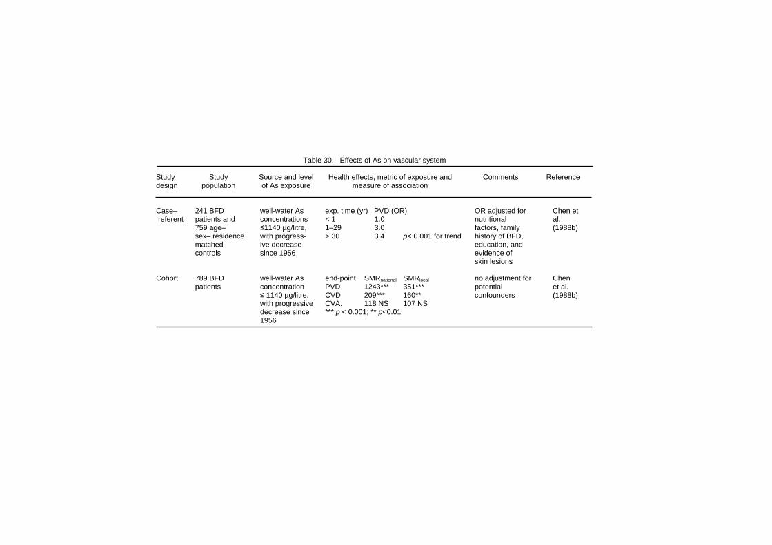
Table 30. Effects of As on vascular system Study Study Source and level Health effects, metric of exposure and Comments Reference design population of As exposure measure of association Case– 241 BFD well-water As exp. time (yr) PVD (OR) OR adjusted for Chen et referent patients and concentrations < 1 1.0 nutritional al. 759 age– ≤1140 µg/litre, 1–29 3.0 factors, family (1988b) sex– residence with progress- > 30 3.4 p< 0.001 for trend history of BFD, matched ive decrease education, and controls since 1956 evidence of skin lesions Cohort 789 BFD well-water As end-point SMRnational SMRlocal no adjustment for Chen patients concentration PVD 1243*** 351*** potential et al. ≤ 1140 µg/litre, CVD 209*** 160** confounders (1988b) with progressive CVA. 118 NS 107 NS decrease since *** p < 0.001; ** p<0.01 1956

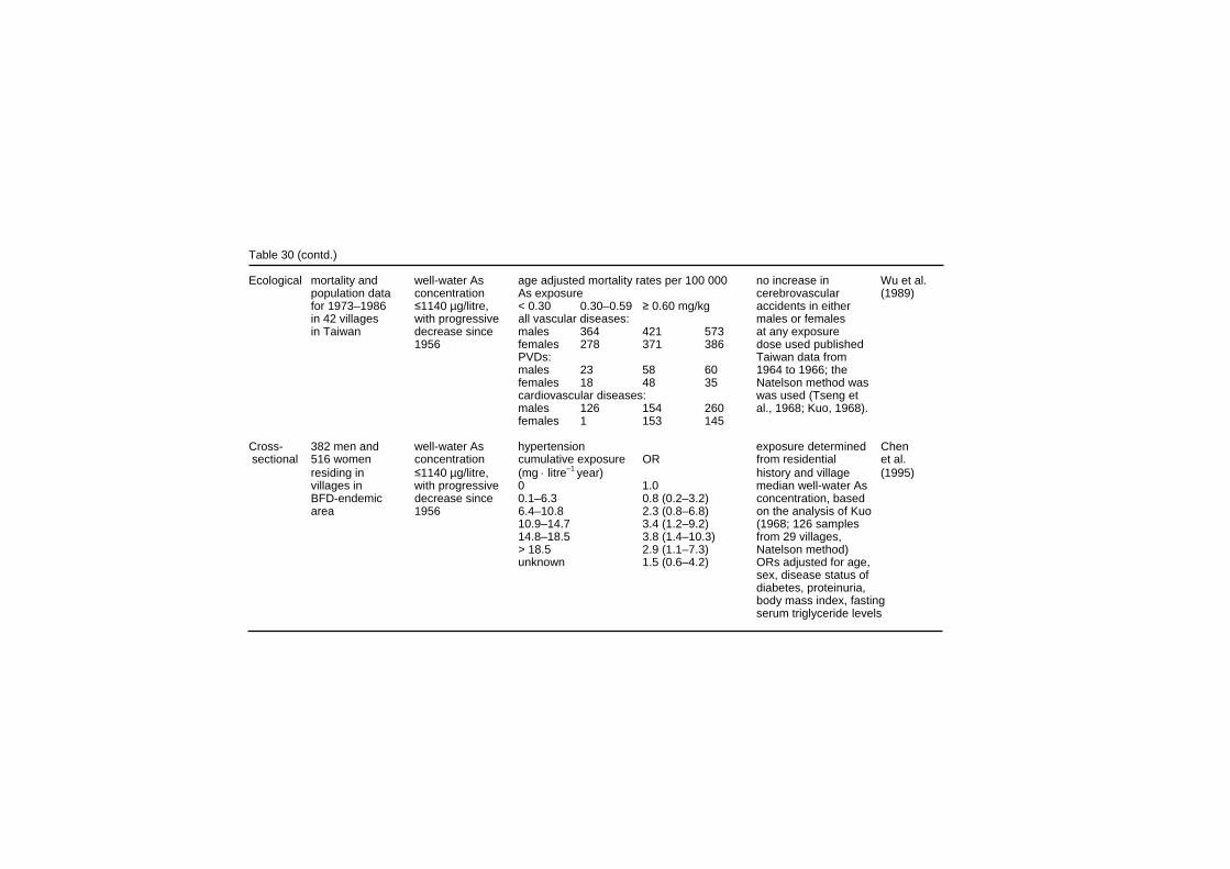
Table 30 (contd.) Ecological mortality and well-water As age adjusted mortality rates per 100 000 no increase in Wu et al. population data concentration As exposure cerebrovascular (1989) for 1973–1986 ≤1140 µg/litre, < 0.30 0.30–0.59 ≥ 0.60 mg/kg accidents in either in 42 villages with progressive all vascular diseases: males or females in Taiwan decrease since males 364 421 573 at any exposure 1956 females 278 371 386 dose used published PVDs: Taiwan data from males 23 58 60 1964 to 1966; the females 18 48 35 Natelson method was cardiovascular diseases: was used (Tseng et males 126 154 260 al., 1968; Kuo, 1968). females 1 153 145 Cross- 382 men and well-water As hypertension exposure determined Chen sectional 516 women concentration cumulative exposure OR from residential et al. residing in ≤1140 µg/litre, (mg ⋅ litre–1 year) history and village (1995) villages in with progressive 0 1.0 median well-water As BFD-endemic decrease since 0.1–6.3 0.8 (0.2–3.2) concentration, based area 1956 6.4–10.8 2.3 (0.8–6.8) on the analysis of Kuo 10.9–14.7 3.4 (1.2–9.2) (1968; 126 samples 14.8–18.5 3.8 (1.4–10.3) from 29 villages, > 18.5 2.9 (1.1–7.3) Natelson method) unknown 1.5 (0.6–4.2) ORs adjusted for age, sex, disease status of diabetes, proteinuria, body mass index, fasting serum triglyceride levels

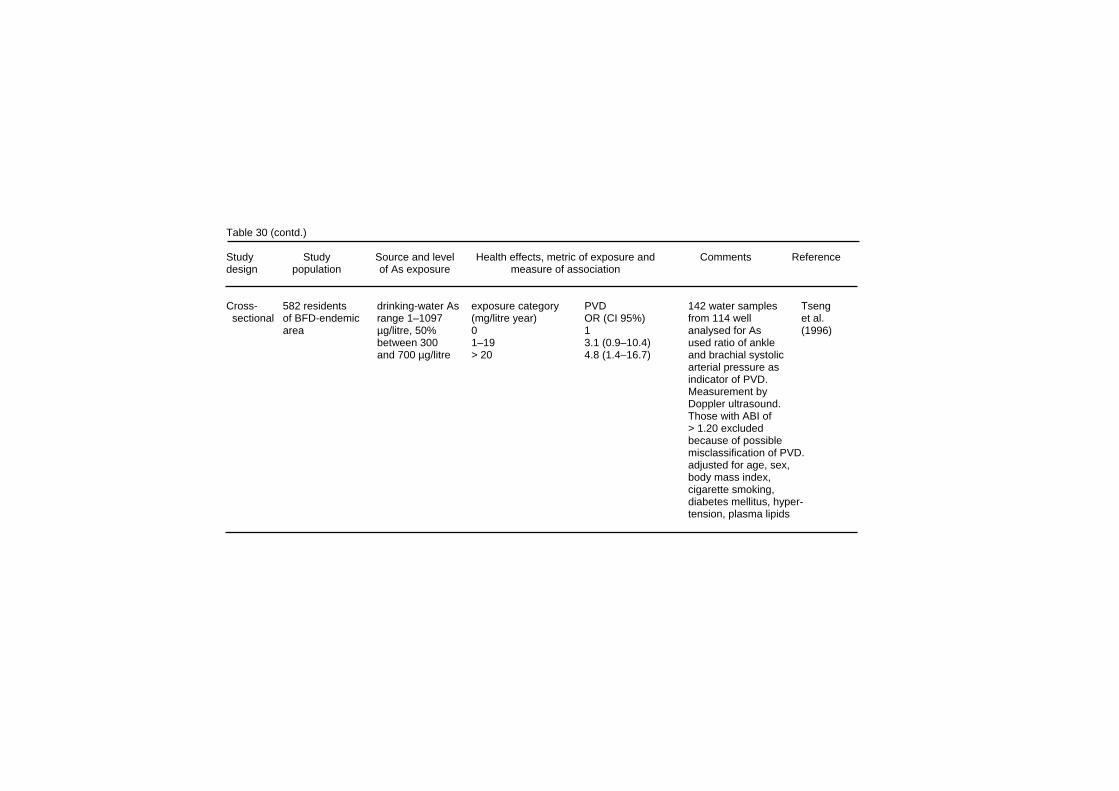
Table 30 (contd.) Study Study Source and level Health effects, metric of exposure and Comments Reference design population of As exposure measure of association Cross- 582 residents drinking-water As exposure category PVD 142 water samples Tseng sectional of BFD-endemic range 1–1097 (mg/litre year) OR (CI 95%) from 114 well et al. area µg/litre, 50% 0 1 analysed for As (1996) between 300 1–19 3.1 (0.9–10.4) used ratio of ankle and 700 µg/litre > 20 4.8 (1.4–16.7) and brachial systolic arterial pressure as indicator of PVD. Measurement by Doppler ultrasound. Those with ABI of > 1.20 excluded because of possible misclassification of PVD. adjusted for age, sex, body mass index, cigarette smoking, diabetes mellitus, hyper- tension, plasma lipids

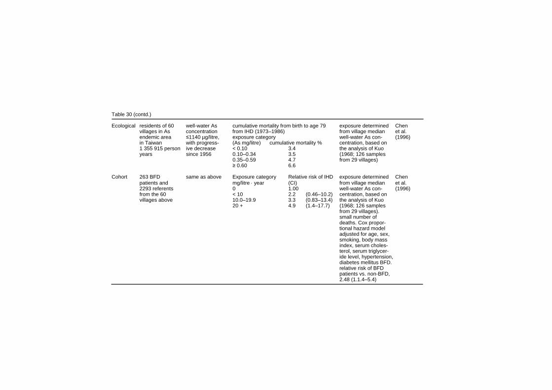
Table 30 (contd.) Ecological residents of 60 well-water As cumulative mortality from birth to age 79 exposure determined Chen villages in As concentration from IHD (1973–1986) from village median et al. endemic area ≤1140 µg/litre, exposure category well-water As con- (1996) in Taiwan with progress- (As mg/litre) cumulative mortality % centration, based on 1 355 915 person ive decrease < 0.10 3.4 the analysis of Kuo years since 1956 0.10–0.34 3.5 (1968; 126 samples 0.35–0.59 4.7 from 29 villages) ≥ 0.60 6.6 Cohort 263 BFD same as above Exposure category Relative risk of IHD exposure determined Chen patients and mg/litre ⋅ year (CI) from village median et al. 2293 referents 0 1.00 well-water As con- (1996) from the 60 < 10 2.2 (0.46–10.2) centration, based on villages above 10.0–19.9 3.3 (0.83–13.4) the analysis of Kuo 20 + 4.9 (1.4–17.7) (1968; 126 samples from 29 villages). small number of deaths. Cox propor- tional hazard model adjusted for age, sex, smoking, body mass index, serum choles- terol, serum triglycer- ide level, hypertension, diabetes mellitus BFD. relative risk of BFD patients vs. non-BFD, 2.48 (1.1.4–5.4)

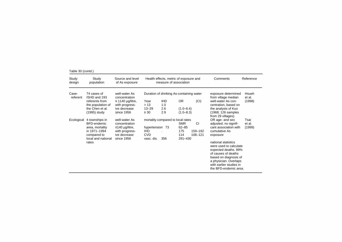
Table 30 (contd.) Study Study Source and level Health effects, metric of exposure and Comments Reference design population of As exposure measure of association Case- 74 cases of well-water As Duration of drinking As-containing water exposure determined Hsueh referent ISHD and 193 concentration from village median et al. referents from ≤ 1140 µg/litre, Year IHD OR (CI) well-water As con- (1998) the population of with progress- > 13 1.0 centration, based on the Chen et al. ive decrease 13–29 2.6 (1.0–6.4) the analysis of Kuo (1995) study since 1956 ≥ 30 2.9 (1.0–8.3) (1968; 126 samples from 29 villages). Ecological 4 townships in well-water As mortality compared to local rates OR age- and sex Tsai BFD-endemic concentration SMR CI adjusted; no signifi- et al. area, mortality ≤140 µg/litre, hypertension 73 62–85 cant association with (1999) in 1971–1994 with progress- IHD . 175 159–192 cumulative As compared to ive decrease CVD 114 108–121 exposure local and national since 1956 vasc. dis. 356 291–430 rates national statistics were used to calculate expected deaths. 99% of causes of deaths based on diagnosis of a physician. Overlaps with earlier studies in the BFD-endemic area.

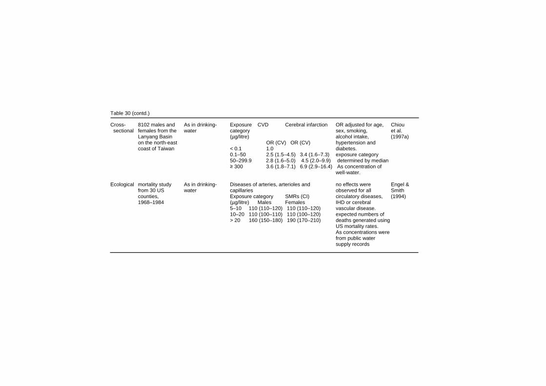
Table 30 (contd.) Cross- 8102 males and As in drinking- Exposure CVD Cerebral infarction OR adjusted for age, Chiou sectional females from the water category sex, smoking, et al. Lanyang Basin (µg/litre) alcohol intake, (1997a) on the north-east OR (CV) OR (CV) hypertension and coast of Taiwan < 0.1 1.0 diabetes. 0.1–50 2.5 (1.5–4.5) 3.4 (1.6–7.3) exposure category 50–299.9 2.8 (1.6–5.0) 4.5 (2.0–9.9) determined by median ≥ 300 3.6 (1.8–7.1) 6.9 (2.9–16.4) As concentration of well-water. Ecological mortality study As in drinking- Diseases of arteries, arterioles and no effects were Engel & from 30 US water capillaries observed for all Smith counties, Exposure category SMRs (CI) circulatory diseases, (1994) 1968–1984 (µg/litre) Males Females IHD or cerebral 5–10 110 (110–120) 110 (110–120) vascular disease. 10–20 110 (100–110) 110 (100–120) expected numbers of > 20 160 (150–180) 190 (170–210) deaths generated using US mortality rates. As concentrations were from public water supply records

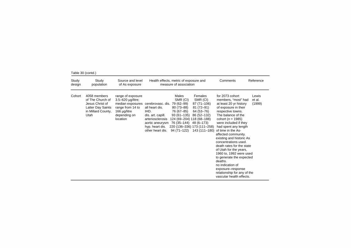
Table 30 (contd.) Study Study Source and level Health effects, metric of exposure and Comments Reference design population of As exposure measure of association Cohort 4058 members range of exposure Males Females for 2073 cohort Lewis of The Church of 3.5–620 µg/litre; SMR (CI) SMR (CI) members, “most” had et al. Jesus Christ of median exposures cerebrovasc. dis. 79 (62–99) 87 (71–106) at least 20 yr history (1999) Latter Day Saints range from 14 to all heart dis. 80 (73–88) 81 (72–91) of exposure in their in Millard County, 166 µg/litre IHD. 76 (67–85) 64 (53–76) respective towns. Utah depending on dis. art. capill. 93 (61–135) 86 (52–132) The balance of the location arteriosclerosis 124 (69–204) 118 (68–188) cohort (n = 1985) aortic aneurysm 76 (35–144) 48 (6–173) were included if they hyp. heart dis. 220 (136–336) 173 (111–258) had spent any length other heart dis. 94 (71–122) 143 (111–180) of time in the As- affected community. existing and historic As concentrations used. death rates for the state of Utah for the years, 1960 to, 1992 were used to generate the expected deaths. no indication of exposure–response relationship for any of the vascular health effects.

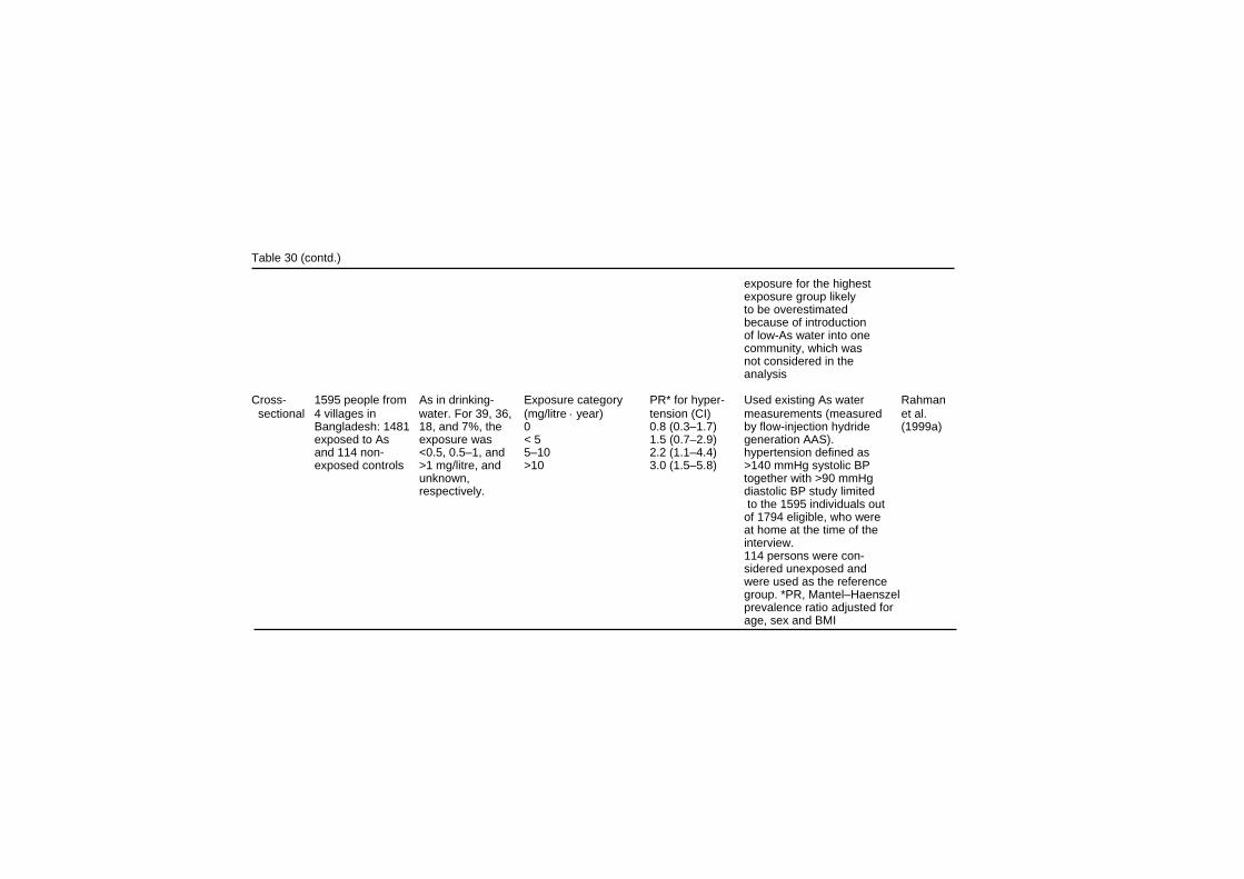
Table 30 (contd.) exposure for the highest exposure group likely to be overestimated because of introduction of low-As water into one community, which was not considered in the analysis Cross- 1595 people from As in drinking- Exposure category PR* for hyper- Used existing As water Rahman sectional 4 villages in water. For 39, 36, (mg/litre ⋅ year) tension (CI) measurements (measured et al. Bangladesh: 1481 18, and 7%, the 0 0.8 (0.3–1.7) by flow-injection hydride (1999a) exposed to As exposure was < 5 1.5 (0.7–2.9) generation AAS). and 114 non- <0.5, 0.5–1, and 5–10 2.2 (1.1–4.4) hypertension defined as exposed controls >1 mg/litre, and >10 3.0 (1.5–5.8) >140 mmHg systolic BP unknown, together with >90 mmHg respectively. diastolic BP study limited to the 1595 individuals out of 1794 eligible, who were at home at the time of the interview. 114 persons were con- sidered unexposed and were used as the reference group. *PR, Mantel–Haenszel prevalence ratio adjusted for age, sex and BMI

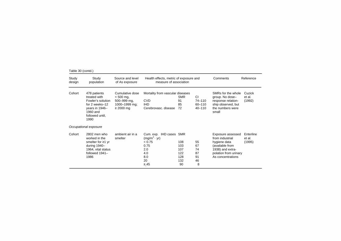
Table 30 (contd.) Study Study Source and level Health effects, metric of exposure and Comments Reference design population of As exposure measure of association Cohort 478 patients Cumulative dose Mortality from vascular diseases SMRs for the whole Cuzick treated with < 500 mg, SMR CI group. No dose– et al. Fowler’s solution 500–999 mg, CVD 91 74–110 response relation- (1992) for 2 weeks–12 1000–1999 mg; IHD 85 60–110 ship observed, but years in 1946– ≥ 2000 mg Cerebrovasc. disease 72 40–110 the numbers were 1960 and small followed until, 1990 Occupational exposure Cohort 2802 men who ambient air in a Cum. exp. IHD cases SMR Exposure assessed Enterline worked in the smelter (mg/m3 ⋅ yr) from industrial et al. smelter for ≥1 yr < 0.75 108 55 hygiene data (1995) during 1940– 0.75 103 67 (available from 1964, vital status 2.0 107 74 1938) and extra- followed 1941– 4.0 122 87 polation from urinary 1986 8.0 128 91 As concentrations 20 132 46 ≥ 45 90 8

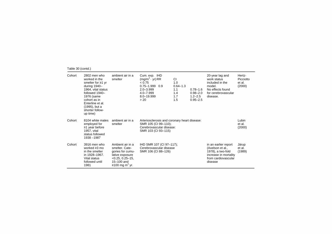
Table 30 (contd.) Cohort 2802 men who ambient air in a Cum. exp. IHD 20-year lag and Hertz- worked in the smelter (mg/m3 ⋅ yr) RR CI work status Picciotto smelter for ≥1 yr < 0.75 1.0 included in the et al. during 1940– 0.75–1.999 0.9 0.64–1.3 model. (2000) 1964, vital status 2.0–3.999 1.1 0.78–1.6 No effects found followed 1940– 4.0–7.999 1.4 0.98–2.0 for cerebrovascular 1976 (same 8.0–19.999 1.7 1.2–2.5 disease. cohort as in > 20 1.5 0.95–2.5 Enterline et al. (1995), but a shorter follow- up time) Cohort 8104 white males ambient air in a Arteriosclerosis and coronary heart disease: Lubin employed for smelter SMR 105 (CI 99–110); et al. ≥1 year before Cerebrovascular disease: (2000) 1957, vital SMR 103 (CI 93–115) status followed 1938 –1987 Cohort 3916 men who Ambient air in a IHD SMR 107 (CI 97–117); in an earlier report Järup worked ≥3 mo smelter. Cate- Cerebrovascular disease (Axelson et al., et al. in the smelter gories for cumu- SMR 106 (CI 88–126) 1978), a two-fold (1989) in 1928–1967. lative exposure increase in mortality Vital status <0.25, 0.25–15, from cardiovascular followed until 15–100 and disease 1981 ≥100 mg m3 yr.

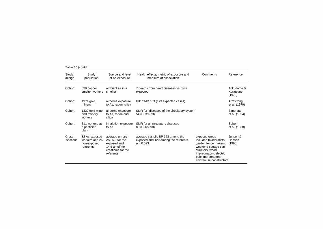
Table 30 (contd.) Study Study Source and level Health effects, metric of exposure and Comments Reference design population of As exposure measure of association Cohort 839 copper ambient air in a 7 deaths from heart diseases vs. 14.9 Tokudome & smelter workers smelter expected Kuratsune (1976) Cohort 1974 gold airborne exposure IHD SMR 103 (173 expected cases) Armstrong miners to As, radon, silica et al. (1979) Cohort 1330 gold mine airborne exposure SMR for “diseases of the circulatory system” Simonato and refinery to As, radon and 54 (CI 39–73) et al. (1994) workers silica Cohort 611 workers at inhalation exposure SMR for all circulatory diseases Sobel a pesticide to As 80 (CI 65–98) et al. (1988) plant Cross- 32 As-exposed average urinary average systolic BP 128 among the exposed group Jensen & sectional workers and 26 As 35.9 for the exposed and 120 among the referents, included taxidermists Hansen non-exposed exposed and p = 0.023 garden fence makers, (1998) referents 14.5 µmol/mol weekend cottage con- creatinine for the structors, wood referents impregnators, electric pole impregnators, new house constructors

Effects on Humans An increasing risk of PVD was also found in an ecological study of 42 villages in the BFD-endemic area in south-western Taiwan (Wu et al., 1989). This study found that age-adjusted mortality rates for PVD increased in an exposure–response relationship with increasing median concentrations of drinking-water arsenic from artesian wells at < 0.30, 0.30–0.59, and ≥0.60 mg/litre for males and females. As this was an ecological study, no individual measures of arsenic exposure were available. In addition, the rates were not adjusted for potential confounders, such as cigarette smoking. A further Taiwanese study attempted to investigate the association between long-term arsenic exposure and PVD morbidity, rather than mortality, using Doppler ultrasound to measure the ankle–brachial index (blood pressure ratio between ankle and brachium, ABI) (Tseng et al., 1996). A cross-sectional study was undertaken, recruiting participants in a previous cohort study. Of the 941 subjects in the original cohort, 582 (62%) took part in the cross-sectional study, so a possible selection bias may have been operating. The study had several advantages over previous Taiwanese studies of BFD, including the use of an objective and more sensitive measure of PVD (i.e. ABI) rather than the physical examination used in previous studies, individual measures of arsenic exposure and the ability to adjust for potential confounders. The study found that the risk of PVD increased with increasing cumulative exposure to arsenic, with a statistically significant increase for the high subgroup (≥20 (mg/litre) year). This association persisted when different cut-off points for ABI were used to diagnose PVD. No association was seen between cumulative arsenic exposure for any of the serum lipids among the 533 individuals studied for these end-points (Tseng et al., 1997). In a case–referent study among 45 healthy residents of the BFD area and 51 referents, it was observed that the perfusion of the big toe, as measured by laser Doppler flowmetry, was weaker among the arsenic-exposed (Tseng et al., 1995). Swedish copper-smelter workers exposed to arsenic (n = 47), with a mean average exposure of 23 years, had a higher prevalence of Raynaud’s phenomenon, indicated by a vasospastic tendency in their fingers after localized cooling, as compared with 48 controls (Lagerkvist et al., 1986). The vasospastic tendency did not disappear

251

EHC 224: Arsenic and Arsenic Compounds during the summer vacation, and thus appeared to be related to long-term rather than short-term exposure to arsenic. However, the vasospastic tendency appeared to diminish over the course of several years, after the exposure to arsenic was reduced (Lagerkvist et al., 1988).

8.4.2 Cardio- and cerebrovascular disease A cohort of 789 BFD patients, followed for 15 years, had a significant increase in mortality from cardiovascular diseases but not cerebrovascular disease (CVD), as compared both with the general Taiwanese population and with residents of the BFD-endemic area (Table 30). However, no adjustment for potential confounders, such as smoking, was undertaken (Chen et al., 1988b). The finding of increasing risk of cardiovascular disease mortality was also found in an ecological study of 42 villages in the BFD-endemic area in south-western Taiwan (Wu et al., 1989). This study found that age-adjusted mortality rates for males and females for all vascular diseases combined increased in a exposure–response relationship with increasing median concentrations of drinking-water arsenic from artesian wells at < 0.30, 0.30–0.59, and ≥0.60 mg/litre. The age-adjusted mortality rates for all vascular diseases and cardiovascular diseases were significantly increased along this exposure gradient. Although the rates increased across exposure groups for CVD, there was no significant exposure–response relationship for either males or females. As this was an ecological study, no individual measures of arsenic exposure were available. Chen et al. (1996) assessed the relationship between ischaemic heart disease (IHD) mortality and long-term arsenic exposure, using two different study designs. The first was an ecological study, which examined the mortality rates of IHD in 60 villages located in a BFD-endemic area in Taiwan. They found a monotonic biological gradient relationship between arsenic exposure in artesian well-water and IHD mortality rates in these villages. The second part of this study was a cohort study of 263 BFD patients and 2293 non-BFD patients recruited from three of the villages with the highest BFD prevalence in Taiwan. This cohort was followed up for an average period of 5 years and an exposure–response relationship between cumulative arsenic intake and mortality from IHD was found. The

252

Effects on Humans relative risks were 2.2, 3.3 and 4.9 respectively for those with cumulative exposures of 0.1–9.9 mg/litre, 10–19.9 mg/litre, and ≥20 mg/litre compared to those without exposure, after adjustment for age, sex, cigarette smoking, BMI, serum levels of cholesterol and triglycerides, hypertension and diabetes (Chen et al., 1996). The exposure to arsenic of 74 cases of IHD (as diagnosed from ECG and a standardized questionnaire), and of 193 referents without IHD, was compared (Hsueh et al., 1998). There was a borderline significant increase of IHD with increasing duration of use of arsenic-containing drinking-water, and a non-significant association with cumulative arsenic exposure. In the most recent ecological study in Taiwan (Tsai et al., 1999), mortality from different causes during 1971–1994 was studied in the area investigated in the first study (Chen et al., 1985), and compared to local rates in both the Chiayi-Tainan county and the whole of Taiwan. The total number of deaths and person-years for the study group was 20 067 and 2 913 382. Age- and sex-specific mortality rates were calculated for each disease for the years 1971–1994. There was an excess mortality from IHD with a standardized mortality ratio (SMR) of 175 (CI 159–192), and a very small but significant excess in the mortality from CVD (SMR 114, CI 108-121; local rates). A study by Chiou et al. (1997a) attempted to elucidate the exposure–response relationship between CVD and ingested arsenic via drinking-water in the north-east coast of Taiwan, an area with elevated drinking-water arsenic concentration, but different from the BFD-endemic area on the south-western coast. The population in this cross-sectional study consisted of 8102 men and women from 3901 households. The CVD status was assessed through initial home interviews and validated by review of medical records; 139 CVD patients were found, including 95 with cerebral infarction. Individual exposure information was obtained by measuring the arsenic concentration in the well-water for each household. Exposure categories were 0, 0.1–50.0, 50.1–299.9, and ≥ 300 µg/litre. This study concluded that a exposure–response relationship exists between the arsenic concentration in well-water and the prevalence of CVD after adjustment for age, sex, hypertension, diabetes mellitus, cigarette smoking and alcohol consumption. This

253

EHC 224: Arsenic and Arsenic Compounds relationship was even more prominent when only the cerebral infarction subgroup was analysed. An ecological mortality study by Engel & Smith (1994) was carried out in 30 counties in the USA with weighted mean concentrations > 5 µg As/litre in drinking-water. This study compared mortality due to several vascular diseases (arteriosclerosis, aortic aneurysm, congenital vascular anomalies, IHD and CVD) in these counties with the expected numbers of deaths generated by US mortality rates. The study found excess mortality rates for males and females for diseases of the arteries, arterioles and capillaries, especially for the highest exposure subgroup (> 20 µg/litre). When this group of diseases was divided into its three main subgroups, the most consistent elevations for the highest exposure group were found for arteriosclerosis mortality, less consistent elevations for mortality from aortic aneurysm, and no elevations for mortality from all other diseases of the arteries, arterioles and capillaries. No elevation in SMRs for either sex in any exposure group was found for all circulatory diseases, IHD or CVD. A cohort study on the relationship between drinking-water arsenic and different causes of mortality was conducted among members of the Church of Jesus Christ of Latter-day Saints (Mormons) in 7 communities in Utah (Lewis et al., 1999). The total number of cohort members was 4058; there were altogether 2203 decedents. By the time of the closing date of the follow-up (1996), 70% of the cohort members had attained the age of 60, and for 67% of the decedents, the time in the cohort was ≥ 40 years. Three hundred individuals (7.4%) were lost to follow-up, and were considered at risk until the last known residence date. Exposure to arsenic was determined from analyses of arsenic in drinking-water, performed by the state health laboratory between 1976 and 1997; the number of the samples for the 7 communities was altogether 151, of which 60 were from the year 1997. The cumulative exposure to arsenic for each individuals was computed on the basis of the residence history from the church records, and the median arsenic concentration of the locality. “Most” of the 2073 members of the cohort had at least 20 years of exposure in their respective town. The balance of the cohort (n = 1985) were included if they had spent “any length of time” in the arsenic affected community. The median drinking-water arsenic concentrations were between 14 and

254

Effects on Humans 166 µg/litre for the different localities, and the maximal recorded concentration was 620 µg/litre. For the community of Hinckley, which provided 29.4% of the cohort participants, and which had the highest median drinking-water concentration, a new water source, low in arsenic, was brought into use in 1981, but only the analytical data before this date were used in the calculations. It is therefore likely that the arsenic exposure represents an overestimation. The observed numbers of deaths from different causes were compared to data for the state of Utah. The expected numbers from the years 1950–1954 were used for those who died (number not given) before 1950, and the expected number from 1990–1992 for those who died after 1992. In men, the overall mortality (SMR 91, CI 86–96) and the mortality from non-malignant respiratory disease were lower than expected (SMR 68, CI 54–85). A similar tendency was observed in women, but was not significant. The study found a deficit in the mortality from CVD, all heart disease and IHD, but a significant excess of deaths from hypertensive heart disease among men and women, and all other heart disease (apart from IHD and hypertensive heart disease) among women. The increases of hypertensive heart diseases showed no exposure–response relationship. The low smoking rates among the church members may have explained the low SMRs for those vascular causes of death related to cigarette smoking (Villanueva & Kogevinas, 1999). Cuzick et al. (1992) studied the causes of death during 1945-1992 among 478 patients treated with Fowler’s solution during the period 1945–1965. Nineteen patients had emigrated and 31 were lost to follow-up; how they were considered in the analysis is not indicated. A total of 188 patients had died before their 85th birthday, and were included in the analysis. Expected values were based on age-, sex-, and calendar year-adjusted rates for England and Wales. The total arsenic dose was calculated from the original treatment records; no data on smoking was available. This study found no association between arsenic exposure and mortality from all circulatory diseases, IHD or CVD. The total exposure of the members of this cohort was lower than that of the major drinking-water cohorts.

255

EHC 224: Arsenic and Arsenic Compounds The relationship between arsenic exposure and vascular diseases has also been studied in some of the occupational cohorts1. These studies are described more fully in section 8.6. In the Tacoma smelter cohort (Enterline et al., 1995) there was a significant excess of IHD, with a weak exposure–response relationship. In a further analysis of this cohort, where attempts were made to adjust for the healthy worker survivor effect, this association was strengthened with a clear exposure–response relationship (Hertz-Picciotto et al., 2000). No significant increase for mortality from CVD was found. In an earlier report on the cohort (Enterline & Marsh, 1982), no excess mortality from heart disease was observed. No significant increase in the mortality from arteriosclerosis and IHD or from CVD was observed among the members of the Montana smelter cohort (Lubin et al., 2000). When the analysis was repeated with an attempt to adjust for the healthy worker survivor effect, there were no changes to the initial findings (Lubin & Fraumeni, 2000). In the first report on the Rönnskär cohort, an arsenic-exposure-related 2-fold increase in the mortality from cardiovascular disease was observed (Axelson et al., 1978). However, in the most recent update, no relationship between exposure to arsenic and IHD or CVD was observed (Järup et al., 1989). In the Japanese smelter cohort (Tokudome & Kuratsune, 1976), there was a deficit of the mortality from heart diseases (7 observed and 14.90 expected cases). Mortality from IHD in a cohort of Australian gold-miners was not different from that expected (Armstrong et al., 1979). In the French gold-miner cohort (Simonato et al., 1994) the mortality from the diseases of the circulatory system was significantly lower than expected. The mortality from the diseases of the circulatory system was also significantly lower than expected in the US pesticide production worker cohort (Sobel et al., 1988).

1 It should be noted, however, that most studies have used SMRs as risk estimates for the exposure response relationships. SMRs are indirectly standardized rate ratios and are thus not directly comparable, unless the risks are homogenous over age strata, or the age structure is similar in the subgroups compared. This is of particular concern for cumulative exposure estimates where there is an inherent heterogeneity in age over exposure subgroups. However, when there are large differences in risk between exposure categories, this theoretical objection is probably less important.

256

Effects on Humans

8.4.3 Hypertension A cross-sectional study was performed by Chen et al. (1995) to examine the association between long-term exposure to inorganic arsenic and the prevalence of hypertension (Table 30). Hypertension was defined as a systolic blood pressure > 160 mmHg or diastolic blood pressure > 95 mmHg, or a reported history of hypertension regularly treated with antihypertensive drugs. Researchers studied a total of 382 men and 516 women residing in villages in the BFD-endemic area in Taiwan, representing 83% of those invited to take part. The age-adjusted prevalence of hypertension was 17.3% (95% CI 13.1-21.5) for men and 18.0% (95% CI 14.1–21.9) for women. The long-term arsenic exposure was calculated from the history of artesian well-water consumption obtained through standardized interviews based on a structured questionnaire and the arsenic concentrations in well-water measured in the 1960s (Kuo, 1968; Natelson method). In this study, residents in the BFD-endemic area had a significantly increased age- and sex-adjusted prevalence of hypertension compared with residents in non-endemic areas. Prevalence odds ratios (POR) for hypertension appeared to follow a exposure–response relationship, as they increased significantly with cumulative arsenic exposures. Odds ratios for the three highest categories remained statistically significant after adjustment for age, sex, diabetes mellitus, proteinuria, body mass index (BMI) and serum triglyceride level (Chen et al., 1995). There was a statistically significant deficit in the mortality from hypertension in the update of the ecological study in Taiwan (Tsai et al., 1999), with an SMR of 73 (CI 62–83). It should be noted that there was, however, an excess mortality from IHD, and that the number of deaths from hypertension itself was unusually high (239 deaths, whereas there were only 283 deaths from IHD). A study by Rahman et al. (1999a) in Bangladesh compared the prevalence of hypertension (assessed by blood pressure measure-ments) among residents with arsenic exposure and those without. A total of 1481 subjects exposed to arsenic-contaminated drinking-water and 114 unexposed subjects were analysed for their time-weighted mean arsenic levels and divided into categories: 0 mg/litre (control) (no detection limit given), < 0.5 mg/litre, 0.5–1.0 mg/litre and > 1.0 mg/litre, and alternatively as cumulative exposures of 0,

257

EHC 224: Arsenic and Arsenic Compounds < 1.0, 1.0–5.0, 5.0–10.0, and > 10.0 (mg/litre) ⋅ year. These exposure categories were assessed with respect to their prevalence of hypertension (a systolic blood pressure of ≥140 mmHg in combi-nation with a diastolic blood pressure of ≥90 mg Hg). It was found that the prevalence ratios, adjusted for age, sex, and BMI, were 1.2, 2.2, 2.5, and 0.8, 1.5, 2.2, and 3.0 in relation to arsenic exposure in mg/litre and (mg/litre) ⋅ year respectively. The exposure–response relationships were significant (p < 0.001) for both series of risk estimates. In a study among a group of 40 Danish workers exposed to arsenic (average urinary arsenic level three times that of the referents), the systolic blood pressure was found to be 8 mmHg higher than that among referents (p = 0.023) (Jensen & Hansen, 1998).

8.5 Diabetes mellitus Lai et al. (1994) assessed the relationship between ingested inorganic arsenic and prevalence of diabetes mellitus in a cross-sectional study (Table 30). The authors examined 891 adults residing in the BFD-endemic area in Taiwan. Diabetic status was determined through oral glucose tolerance test or a history of diabetes regularly treated with sulfonylurea agents or insulin. The rate of diabetes among the 891 study subjects was twice that of the rates previously reported for residents in Taipei and the entire Taiwan population, after adjustment for age and sex. The authors also estimated the cumulative exposure to arsenic from a detailed history of residential addresses and duration of artesian well-water obtained through standardized questionnaires and personal interviews. Prevalence of diabetes, after adjusting for age, sex, BMI and physical activity level increased with increasing arsenic exposure with odds ratios of 6.6 and 10.1 for the two cumulative exposure groups respectively (0.1-15 and > 15 (mg/litre) ⋅ year). There was an excess mortality from diabetes among the arsenic exposed population in the most recent ecological study in Taiwan (Tsai et al., 1999; for study description, see section 8.7 on cancer), with an SMR of 135 (CI 116–155).

258

Effects on Humans In a study in Bangladesh, people with skin keratosis in six districts with arsenic-contaminated drinking-water were identified as a study group. This group was then divided into three drinking-water arsenic concentration strata, on the basis of mean arsenic level in drinking-water over the lifetime of the subject. A non-exposed group was identified in a door-to-door survey in Dhaka (Rahman et al., 1998). This study showed elevated risks for diabetes for those exposed to arsenic in their drinking-water (prevalence ratio = 5.9 after controlling for age, BMI, and sex) as compared with the unexposed. There was also a strong exposure–response relationship among the three exposure subgroups (Table 31).2 In another cross-sectional study in the same villages (Rahman et al., 1999b; for study description see section 8.4.3, Rahman et al., 1999a), The prevalence ratios of glucosuria, adjusted for age and sex, were 0.4, 0.9, 1.2 and 1.7 for individuals without skin lesions, and 0.8, 1.7, 2.1, and 2.9 for those with skin lesions, in the cumulative arsenic exposure categories of > 1, 1–5, 5–10, and > 10 (mg/litre) ⋅ year, respectively. The exposure–response relation-ships were significant (p < 0.001) for both series groups. In the Utah mortality study (Lewis et al., 1999; see section 8.4.2 above) no significant excess number of deaths from diabetes mellitus was found in men (SMR = 79) or women (SMR = 123). However, in the USA diabetes is a condition with a low case fatality rate, so an association with diabetes mellitus may not be observed in a mortality study. In order to investigate the role of occupational arsenic exposure in the pathogenesis of diabetes mellitus, Rahman & Axelson (1995) conducted a small (12 exposed cases) case–referent study in the Rönnskär cohort (Axelson et al., 1978). An elevated risk of diabetes mellitus associated with arsenic exposure was observed: OR 2.0, 4.2, and 7.0 for the exposure categories << 0.5, < 0.5 and > 0.5 mg/m3; confidence intervals for all included unity, and the trend was of borderline significance (p = 0.03).

2 After the Task Group meeting, the secretariat became aware of a further study reporting an association between exposure to arsenic in drinking water and diabetes mellitus (Tseng et al., 2000a,b)

259

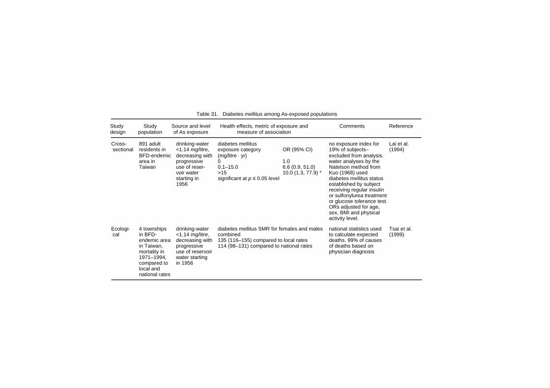
Table 31. Diabetes mellitus among As-exposed populations Study Study Source and level Health effects, metric of exposure and Comments Reference design population of As exposure measure of association Cross- 891 adult drinking-water diabetes mellitus no exposure index for Lai et al. sectional residents in <1.14 mg/litre, exposure category OR (95% CI) 19% of subjects– (1994) BFD-endemic decreasing with (mg/litre ⋅ yr) excluded from analysis. area in progressive 0 1.0 water analyses by the Taiwan use of reser- 0.1–15.0 6.6 (0.9, 51.0) Natelson method from voir water >15 10.0 (1.3, 77.9) * Kuo (1968) used starting in significant at p ≤ 0.05 level diabetes mellitus status 1956 established by subject receiving regular insulin or sulfonylurea treatment or glucose tolerance test. ORs adjusted for age, sex, BMI and physical activity level. Ecologi- 4 townships drinking-water diabetes mellitus SMR for females and males national statistics used Tsai et al. cal in BFD- <1.14 mg/litre, combined to calculate expected (1999) endemic area decreasing with 135 (116–155) compared to local rates deaths. 99% of causes in Taiwan, progressive 114 (98–131) compared to national rates of deaths based on mortality in use of reservoir physician diagnosis 1971–1994, water starting compared to in 1956 local and national rates

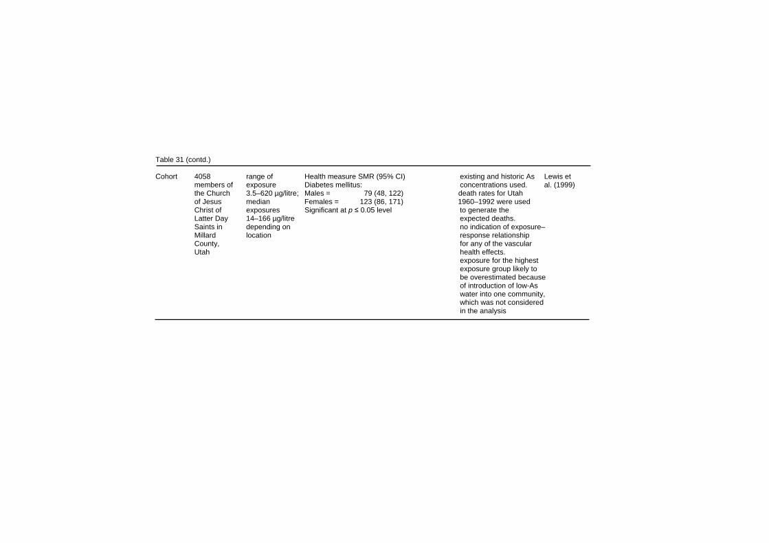
Table 31 (contd.) Cohort 4058 range of Health measure SMR (95% CI) existing and historic As Lewis et members of exposure Diabetes mellitus: concentrations used. al. (1999) the Church 3.5–620 µg/litre; Males = 79 (48, 122) death rates for Utah of Jesus median Females = 123 (86, 171) 1960–1992 were used Christ of exposures Significant at p ≤ 0.05 level to generate the Latter Day 14–166 µg/litre expected deaths. Saints in depending on no indication of exposure– Millard location response relationship County, for any of the vascular Utah health effects. exposure for the highest exposure group likely to be overestimated because of introduction of low-As water into one community, which was not considered in the analysis

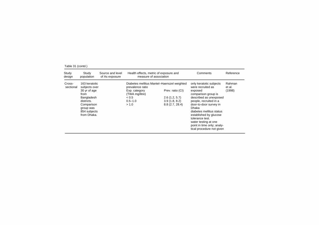
Table 31 (contd.) Study Study Source and level Health effects, metric of exposure and Comments Reference design population of As exposure measure of association Cross- 163 keratotic Diabetes mellitus Mantel–Haenszel weighted only keratotic subjects Rahman sectional subjects over prevalence ratio were recruited as et al. 30 yr of age Exp. category Prev. ratio (CI) exposed (1998) from (TWA mg/litre) comparison group is Bangladesh < 0.5 2.6 (1.2, 5.7) described as unexposed districts. 0.5–1.0 3.9 (1.8, 8.2) people, recruited in a Comparison > 1.0 8.8 (2.7, 28.4) door-to-door survey in group was Dhaka 854 subjects diabetes mellitus status from Dhaka. established by glucose tolerance test. water testing at one point in time only; analy- tical procedure not given

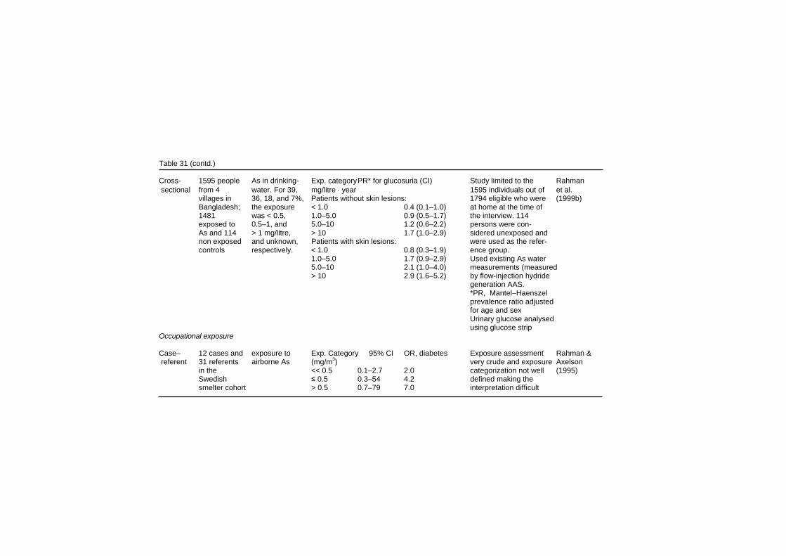
Table 31 (contd.) Cross- 1595 people As in drinking- Exp. category PR* for glucosuria (CI) Study limited to the Rahman sectional from 4 water. For 39, mg/litre ⋅ year 1595 individuals out of et al. villages in 36, 18, and 7%, Patients without skin lesions: 1794 eligible who were (1999b) Bangladesh; the exposure < 1.0 0.4 (0.1–1.0) at home at the time of 1481 was < 0.5, 1.0–5.0 0.9 (0.5–1.7) the interview. 114 exposed to 0.5–1, and 5.0–10 1.2 (0.6–2.2) persons were con- As and 114 > 1 mg/litre, > 10 1.7 (1.0–2.9) sidered unexposed and non exposed and unknown, Patients with skin lesions: were used as the refer- controls respectively. < 1.0 0.8 (0.3–1.9) ence group. 1.0–5.0 1.7 (0.9–2.9) Used existing As water 5.0–10 2.1 (1.0–4.0) measurements (measured > 10 2.9 (1.6–5.2) by flow-injection hydride generation AAS. *PR, Mantel–Haenszel prevalence ratio adjusted for age and sex Urinary glucose analysed using glucose strip Occupational exposure Case– 12 cases and exposure to Exp. Category 95% CI OR, diabetes Exposure assessment Rahman & referent 31 referents airborne As (mg/m3) very crude and exposure Axelson in the << 0.5 0.1–2.7 2.0 categorization not well (1995) Swedish ≤ 0.5 0.3–54 4.2 defined making the smelter cohort > 0.5 0.7–79 7.0 interpretation difficult

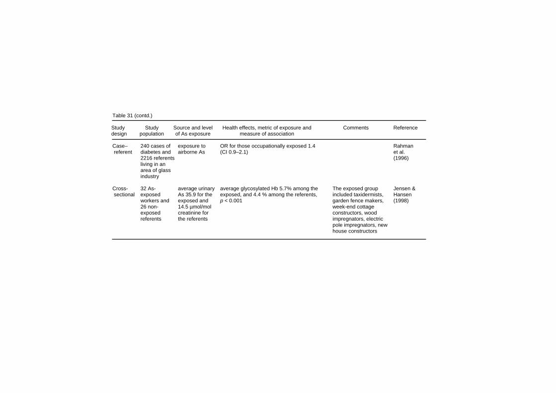
Table 31 (contd.) Study Study Source and level Health effects, metric of exposure and Comments Reference design population of As exposure measure of association Case– 240 cases of exposure to OR for those occupationally exposed 1.4 Rahman referent diabetes and airborne As (CI 0.9–2.1) et al. 2216 referents (1996) living in an area of glass industry Cross- 32 As- average urinary average glycosylated Hb 5.7% among the The exposed group Jensen & sectional exposed As 35.9 for the exposed, and 4.4 % among the referents, included taxidermists, Hansen workers and exposed and p < 0.001 garden fence makers, (1998) 26 non- 14.5 µmol/mol week-end cottage exposed creatinine for constructors, wood referents the referents impregnators, electric pole impregnators, new house constructors

Effects on Humans Rahman et al. (1996) also conducted a case–referent analysis in the glass industry area in Sweden on 240 individuals who had diabetes as the underlying or contributing cause of death on the death certificate, and 2216 controls who died of other causes during 1950-1982. They found a slightly elevated risk of dying from diabetes among glasswork employees considered to be exposed to arsenic on the basis of their occupational histories (OR 1.4, 95% CI 0.9–2.2). In a study among a group of 40 Danish workers exposed to arsenic (average urinary arsenic level 22.3 µmol/mol creatinine; twice that of the referents), the blood concentration of glycosylated haemoglobin (used as a marker of long-term blood glucose level) was 25% higher (p < 0.001) than that among referents, and showed a significant trend with increasing urinary arsenic concentrations (Jensen & Hansen, 1998).

8.6 Neurotoxicity Polyneuropathy is often among the sequelae of an acute oral arsenic poisoning (Heyman et al., 1956), and was reported as early as the 18th century (for references see Geyer, 1898). Sensory nerve (median, ulnar and sural nerves) conduction is often affected more (absent or low action potentials) than the motor nerves (primarily low amplitude in action potential, slowing or prolonged nerve conduction velocity) (Murphy et al., 1981; Oh, 1991). The conduction velocity may decrease during several weeks after short-term exposure, but conduction velocity changes were observed 3 days after a large dose (Ramirez-Campos et al., 1998). If the patient survives, the electrophysiological changes show a slow recovery. Histological examination of the nerves involved typically reveals wallerian degeneration (Murphy et al., 1981; Goebel et al., 1990; Oh, 1991). More rarely, arsenic intoxication may also lead into prolonged toxic encephalopathy (Freeman & Couch, 1956; Fincher & Koerker, 1987). Cases with neuropsychological and neurophysio-logical damage after occupational exposure to arsenic have also been described (Becket et al., 1986; Bolla-Wilson & Bleecker, 1987; Morton & Caron, 1989). Few epidemiological studies have investigated whether a lower level long-term exposure to arsenic may also lead to neurotoxicity.

265

EHC 224: Arsenic and Arsenic Compounds Hindmarsh et al. (1977) assessed the effect of drinking-water with high arsenic concentration on electromyographic abnormalities. Out of 110 persons exposed to elevated arsenic concentrations in drinking-water, 32 were studied using electromyography (EMG), and compared to 12 non-exposed referents. There was a positive relationship between EMG abnormalities and well and hair arsenic concentrations. Among those using water with > 1 mg As/litre, the frequency of EMG abnormalities was 50%. In a cross-sectional study on 211 people in Fairbanks, Alaska, “brief clinical investigation” of peripheral nervous system function (not specified) did not reveal neuropathy related to estimated daily arsenic dose from drinking-water; the latter was estimated from well-water arsenic concentration, and reported use of well-water and bottled water. The estimated average arsenic exposure in the highest exposure category was 0.3 mg/day (Harrington et al., 1978). Workers at a copper-smelting plant exposed to As2O3 were examined for peripheral neuropathy (Feldman et al., 1979). A total of 70 factory workers and 41 non-arsenic workers were evaluated. Among the exposed workers there was an association between exposure to arsenic (quantitated in urine, hair and nails) and a higher number of peripheral neuropathological disorders (sensory and motor neuropathy) and electrophysiological abnormalities (reduced nerve conduction velocity and amplitude measurements). Of the arsenic-exposed workers 30% had sensory and 13% motor neuropathy, compared to 12% of the non-exposed group with sensory and none with motor neuropathy. Power station workers were exposed to fuel coal with a high content of arsenic (Buchancova et al., 1998). The author describes a variety of clinical symptoms potentially associated with arsenic: sensory and motor polyneuropathy, pseudoneurasthenic syndrome, toxic encephalopathy and nasal septum perforation. However, workers were also exposed to manganese and lead, both known neurotoxic chemicals. A girl who was accidentally exposed to copper acetoarsenite (Paris green) used as a pesticide had severe clinical signs of arsenic poisoning including Mees’ bands in fingers and toenails, encepha-lopathy, epileptic seizures and demyelinating polyneuropathy with a

266

Effects on Humans severe motor deficit (Brouwer et al., 1992). Although her family was also exposed, as indicated by elevated arsenic in their urine, they remained asymptomatic. Further analysis indicated that she was deficient in 5,10-methylene-tetrahydrofolate reductase (MTHFR), which is involved in the conversion of 5,10-methylene tetrahydrofolate to 5-methyl tetrahydrofolate and is important for myelin biosynthesis. MTFH deficiency may have led to decreased synthesis of S-adenosylmethione (SAM), which is a methyl donor for arsenic methylation, and thus to increased toxicity of arsenic.

8.7 Cancer

8.7.1 Exposure via inhalation Investigation into elevated cancer risk amongst copper-smelter workers was initiated during the early 1960s. The emphasis in the studies on inhalation exposure to arsenic and cancer has been in respiratory cancer, mainly lung cancer (Table 32).

8.7.1.1 Lung cancer a) Non-ferrous smelters There are three occupational cohorts in which exposure assessments allow evaluation of the relationship between exposure to arsenic and lung cancer, namely those of the copper smelters in Tacoma, Washington (USA), Anaconda, Montana (USA), and Rönnskär (Sweden). These studies are described below in more detail, and other studies on the relationship between arsenic exposure and cancer are presented in a more condensed form. Results from the Tacoma copper smelter have been published in a series of papers (Pinto & Bennett, 1963; Pinto et al., 1977, 1978; Enterline & Marsh, 1980, 1982; Enterline et al., 1987a, 1995). In the most recent update (Enterline et al., 1995), the vital status of 2802 men who worked at the smelter for a year or more during the period 1940–1964 was followed for the period 1941–1986; exposure assessment was extended to 1984. The vital status was determined for 98.5% of the cohort, and of the 1583 known deaths, death certificates were obtained for 96.6%. The expected numbers of deaths for various diseases were calculated from age- and time-

267

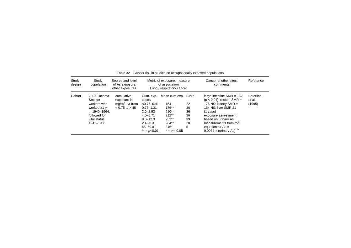
Table 32. Cancer risk in studies on occupationally exposed populations Study Study Source and level Metric of exposure, measure Cancer at other sites; Reference design population of As exposure; of association comments other exposures Lung / respiratory cancer Cohort 2802 Tacoma cumulative Cum. exp. Mean cum.exp. SMR large intestine SMR = 162 Enterline Smelter exposure in cases (p < 0.01); rectum SMR = et al. workers who mg/m3 ⋅ yr from <0.75–0.41 154 22 176 NS; kidney SMR = (1995) worked ≥1 yr < 0.75 to > 45 0.75–1.31 176** 30 164 NS; liver SMR 21 in 1940–1964, 2.0–2.93 210** 36 (1 case) followed for 4.0–5.71 212** 36 exposure assessment vital status 8.0–12.3 252** 39 based on urinary As 1941–1986 20–28.3 284** 20 measurements from the 45–59.0 316* 5 equation air As = ** = p<0.01; * = p < 0.05 0.0064 × (urinary As)1.942

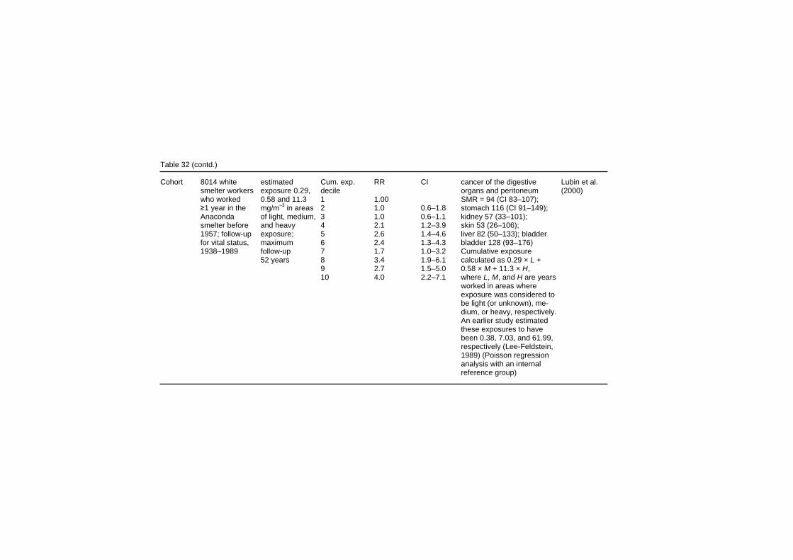
Table 32 (contd.) Cohort 8014 white estimated Cum. exp. RR CI cancer of the digestive Lubin et al. smelter workers exposure 0.29, decile organs and peritoneum (2000) who worked 0.58 and 11.3 1 1.00 SMR = 94 (CI 83–107); ≥1 year in the mg/m–3 in areas 2 1.0 0.6–1.8 stomach 116 (CI 91–149); Anaconda of light, medium, 3 1.0 0.6–1.1 kidney 57 (33–101); smelter before and heavy 4 2.1 1.2–3.9 skin 53 (26–106); 1957; follow-up exposure; 5 2.6 1.4–4.6 liver 82 (50–133); bladder for vital status, maximum 6 2.4 1.3–4.3 bladder 128 (93–176) 1938–1989 follow-up 7 1.7 1.0–3.2 Cumulative exposure 52 years 8 3.4 1.9–6.1 calculated as 0.29 × L + 9 2.7 1.5–5.0 0.58 × M + 11.3 × H, 10 4.0 2.2–7.1 where L, M, and H are years worked in areas where exposure was considered to be light (or unknown), me- dium, or heavy, respectively. An earlier study estimated these exposures to have been 0.38, 7.03, and 61.99, respectively (Lee-Feldstein, 1989) (Poisson regression analysis with an internal reference group)

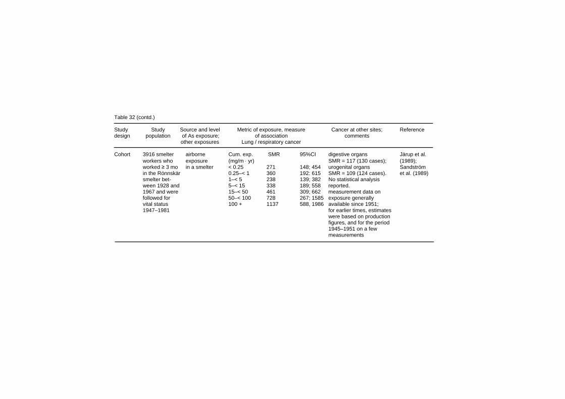
Table 32 (contd.) Study Study Source and level Metric of exposure, measure Cancer at other sites; Reference design population of As exposure; of association comments other exposures Lung / respiratory cancer Cohort 3916 smelter airborne Cum. exp. SMR 95%CI digestive organs Järup et al. workers who exposure (mg/m ⋅ yr) SMR = 117 (130 cases); (1989); worked ≥ 3 mo in a smelter < 0.25 271 148; 454 urogenital organs Sandström in the Rönnskär 0.25–< 1 360 192: 615 SMR = 109 (124 cases). et al. (1989) smelter bet- 1–< 5 238 139; 382 No statistical analysis ween 1928 and 5–< 15 338 189; 558 reported. 1967 and were 15–< 50 461 309; 662 measurement data on followed for 50–< 100 728 267; 1585 exposure generally vital status 100 + 1137 588, 1986 available since 1951; 1947–1981 for earlier times, estimates were based on production figures, and for the period 1945–1951 on a few measurements

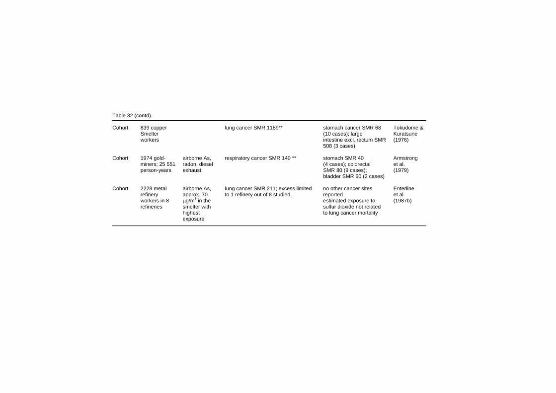
Table 32 (contd). Cohort 839 copper lung cancer SMR 1189** stomach cancer SMR 68 Tokudome & Smelter (10 cases); large Kuratsune workers intestine excl. rectum SMR (1976) 508 (3 cases) Cohort 1974 gold- airborne As, respiratory cancer SMR 140 ** stomach SMR 40 Armstrong miners; 25 551 radon, diesel (4 cases); colorectal et al. person-years exhaust SMR 80 (9 cases); (1979) bladder SMR 60 (2 cases) Cohort 2228 metal airborne As, lung cancer SMR 211; excess limited no other cancer sites Enterline refinery approx. 70 to 1 refinery out of 8 studied. reported et al. workers in 8 µg/m3 in the estimated exposure to (1987b) refineries smelter with sulfur dioxide not related highest to lung cancer mortality exposure

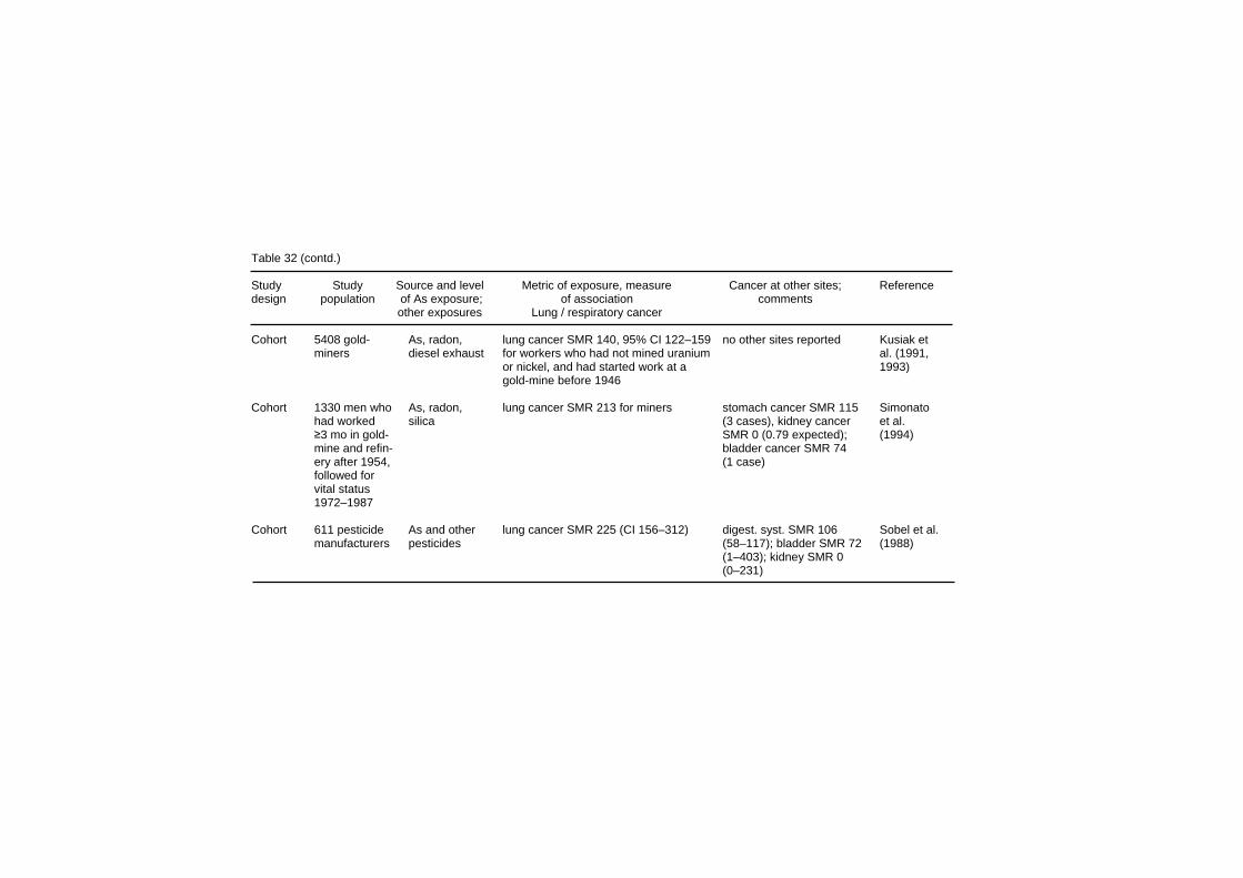
Table 32 (contd.) Study Study Source and level Metric of exposure, measure Cancer at other sites; Reference design population of As exposure; of association comments other exposures Lung / respiratory cancer Cohort 5408 gold- As, radon, lung cancer SMR 140, 95% CI 122–159 no other sites reported Kusiak et miners diesel exhaust for workers who had not mined uranium al. (1991, or nickel, and had started work at a 1993) gold-mine before 1946 Cohort 1330 men who As, radon, lung cancer SMR 213 for miners stomach cancer SMR 115 Simonato had worked silica (3 cases), kidney cancer et al. ≥3 mo in gold- SMR 0 (0.79 expected); (1994) mine and refin- bladder cancer SMR 74 ery after 1954, (1 case) followed for vital status 1972–1987 Cohort 611 pesticide As and other lung cancer SMR 225 (CI 156–312) digest. syst. SMR 106 Sobel et al. manufacturers pesticides (58–117); bladder SMR 72 (1988) (1–403); kidney SMR 0 (0–231)

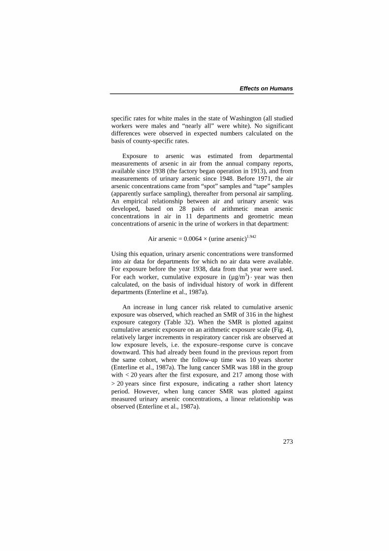
Effects on Humans specific rates for white males in the state of Washington (all studied workers were males and “nearly all” were white). No significant differences were observed in expected numbers calculated on the basis of county-specific rates. Exposure to arsenic was estimated from departmental measurements of arsenic in air from the annual company reports, available since 1938 (the factory began operation in 1913), and from measurements of urinary arsenic since 1948. Before 1971, the air arsenic concentrations came from “spot” samples and “tape” samples (apparently surface sampling), thereafter from personal air sampling. An empirical relationship between air and urinary arsenic was developed, based on 28 pairs of arithmetic mean arsenic concentrations in air in 11 departments and geometric mean concentrations of arsenic in the urine of workers in that department:

Air arsenic = 0.0064 × (urine arsenic)1.942

Using this equation, urinary arsenic concentrations were transformed into air data for departments for which no air data were available. For exposure before the year 1938, data from that year were used. For each worker, cumulative exposure in (µg/m3) ⋅ year was then calculated, on the basis of individual history of work in different departments (Enterline et al., 1987a). An increase in lung cancer risk related to cumulative arsenic exposure was observed, which reached an SMR of 316 in the highest exposure category (Table 32). When the SMR is plotted against cumulative arsenic exposure on an arithmetic exposure scale (Fig. 4), relatively larger increments in respiratory cancer risk are observed at low exposure levels, i.e. the exposure–response curve is concave downward. This had already been found in the previous report from the same cohort, where the follow-up time was 10 years shorter (Enterline et al., 1987a). The lung cancer SMR was 188 in the group with < 20 years after the first exposure, and 217 among those with > 20 years since first exposure, indicating a rather short latency period. However, when lung cancer SMR was plotted against measured urinary arsenic concentrations, a linear relationship was observed (Enterline et al., 1987a).

273

EHC 224: Arsenic and Arsenic Compounds An elevated risk of lung cancer among workers in the Anaconda copper smelter in Montana was originally reported by Lee & Fraumeni (1969). Updates and further cohort and nested case–referent analyses were published later (Lubin et al., 1981; Welch et al., 1982; Brown & Chu, 1983a,b; Lee-Feldstein, 1983, 1986, 1989; Lubin et al., 2000). The study population of the latest cohort update (Lubin et al., 2000) consisted of 8014 white males, who were employed for ≥12 months before 1957. Their vital status was followed from 1 January 1938 to 31 December 1987; a total of 4930 (63%) were deceased, including 446 from respiratory cancer. The vital status at the end of the follow-up period was not known for 1175 workers (15%), and they were assumed to be alive at the end of the study period (except the 81 workers born before 1900, who were assumed to have died). Industrial hygiene data (702 measurements), collected between 1943 and 1958, were used to categorize each work site to an exposure category on a scale 1–10, and work areas were then grouped as representing “light”, “medium” or “heavy” exposure. Based in addition on estimates of workers’ daily exposure time, time-weighted average (TWA) exposures for each category were created, and were considered to be 0.29, 0.58 and 11.3 mg/m3 arsenic for the “light”, “medium”, and “heavy” exposure category (Lubin et al., 2000). It should be noted that in earlier reports on this cohort the TWA exposure estimates used were different, notably for the “heavy” exposure category (0.38, 7.03, and 61.99 mg/m3, respect-ively). For each worker, the cumulative exposure was estimated from the time of working in different work areas. The authors note that industrial hygiene measurements were actually available for less than half of the 29 working areas; no data were collected before 1943, and the measurements were often performed when an industrial hygiene control measure was instituted or after a process change occurred, and most often in areas where arsenic was thought to be a hazard. The locations for sampling were not randomly selected. Altogether 446 deaths from respiratory cancer (SMR 155; CI 141–170) were observed. A trend of increasing risk with increasing estimated exposure was seen (Table 32); the risk increased linearly with time of employment in each exposure category. The elevated lung cancer incidence among workers of the Rönnskär smelter in northern Sweden was originally reported in a

274

Effects on Humans population-based case–referent study in St Örjan parish in 1978 (Axelson et al., 1978). Since then, studies using both cohort and case–referent approaches have been published (Wall, 1980; Pershagen et al., 1981, 1987; Järup et al., 1989; Sandström et al., 1989; Järup & Pershagen, 1991; Sandström & Wall, 1993). The cohort consisted of 3916 male smelter workers, who had worked for at least 3 months at the smelter between 1928 and 1967. The vital status of all but 15 (0.4%) of them was verified. Mortality of different causes, as defined on death certificates, was compared to local rates. Reference rates were not available for the period before 1951, but the contribution of deaths during this period (89 out of a total of 1275, i.e. 7%) was minor. Air concentrations of arsenic were estimated by the factory industrial hygienists. The first measurements were carried out in 1945, and from 1951 exposure data were more generally available; production figures were used to extrapolate exposures before 1951. Each work site was characterized by an exposure level during three consecutive time periods, and the workers’ cumulative exposure was assessed on the basis of their working history in these different work sites. The SMRs were very similar whether they were calculated with no latency, 10 years minimum latency or 10 years minimum latency with exposure lagged 5 years. A dose-dependent increase in the mortality from lung cancer was observed (Table 32), and a statistically significantly increased risk was observed even in the lowest exposure category, < 0.25 (mg/m3) ⋅ year. A sensitivity analysis showed that the SMRs were fairly robust, particularly among the workers with low and medium exposure (Järup, 1992). Even when the exposures before 1940 were reduced dramatically (assuming there was a large overestimation of the early exposures), these SMRs changed only marginally. As expected, the SMRs in the highest exposure group increased as the early exposures were reduced. An overestimation of the early exposures would thus tend to decrease the strength of the exposure–response association. However, in a nested case–referent study on the interaction between smoking and arsenic exposure as cancer-causing agents (Järup & Pershagen, 1991), little increased risk of lung cancer due to arsenic exposure was observed among smokers or non-smokers in exposure categories < 15 (mg/m3) ⋅ year. Little difference was observed in the SMRs for workers hired before 1940, in 1940–1949, or after 1949, when the estimated level of exposure was similar, meaning that a

275

EHC 224: Arsenic and Arsenic Compounds longer follow-up did not increase the apparent risk. In most subcohorts, and in the total cohort, the mortality increased with increasing average intensity of exposure, but no clear-cut trend was observed for the duration of exposure. Exposure to sulfur dioxide was also assessed. The lung cancer risk was elevated in all groups exposed to sulfur dioxide, but there was no exposure–response with the estimated cumulative sulfur dioxide exposure. In a cancer incidence study (Sandström et al., 1989), partly overlapping with the mortality study, the cancer risk of the smelter workers over a moving 5-year period was observed to decrease steadily from 1976–1979 to 1980–1984. Further follow-up of an expanded Rönnskär cohort (n = 6 334) by Sandström & Wall (1992) showed a decreasing trend in lung cancer incidence and mortality, but there was still an elevated lung cancer incidence among the workers when compared with Swedish men. A very high excess of lung cancer (SMR 2500; 10 observed and 0.40 expected cases in the heavy exposure category), which was related to duration and level of exposure, was observed in the copper smelter of a Japanese metal refinery (Tokudome & Kuratsune, 1976); the study was prompted by an earlier case–referent study that demonstrated an excess lung cancer rate among copper-smelter workers (Kuratsune et al., 1974). There was an approximately 3-fold increase in the relative death rate from lung cancer among employees of a copper smelter in Utah, in comparison to workers of the same company not employed in the smelter (mainly mine and concentrator workers), and also in comparison to Utah state figures (Rencher et al., 1977). The risk was related to all estimated exposure parameters (cumulative exposure to arsenic, sulfuric acid, lead and copper), and was similar for smokers and non-smokers. This refinery was a part of a cohort study in eight copper smelters (Enterline et al., 1987b), the SMR for respiratory cancer < 20 years since first exposure was 170 (11 deaths), and ≥ 20 years 108 (39 deaths) (reported in Enterline et al., 1995). In this study, the only smelter with an appreciable exposure to arsenic was the Utah one, and this was the only one with a statistically significant excess in lung cancer. b) Pesticide manufacture and application Ott et al. (1974) conducted a proportionate mortality study of decedents who had worked at a factory producing arsenical

276

Effects on Humans pesticides, mainly lead arsenate, calcium arsenate, copper aceto-arsenite and magnesium arsenate. The cause of death of 173 workers who had worked at least 1 day in jobs with presumed arsenic exposure was compared to that of 1809 decedents (age- and calendar-year-adjusted) from the same factory, with no exposure to arsenic or asbestos. The exposure of the workers was analysed from a job exposure matrix covering the working history. The proportionate mortality ratio (PMR) for lung cancer increased with estimated exposure, from a PMR of 200 at an exposure level of 1-1.9 (mg/m3) ⋅ month to a PMR of 700 at the highest cumulative exposure group ≥96 (mg/m3) ⋅ month. Ott et al. (1974) also conducted a cohort study at the pesticide plant. The cohort was expanded and updated through December 1982 (Sobel et al., 1988) to include 611 workers altogether; the mortality was compared to age- and calendar-time standardized data on US white males. A significant excess of lung cancer mortality was observed (35 observed vs. 15.6 expected cases; SMR 225, 95% CI 156–312). The small number of deaths made analyses by duration and latency difficult; analysis by exposure level or cumulative exposure was not reported. In a cohort study of pesticide manufacturing workers in Baltimore, the vital status of 1050 men and 343 women was followed from 1946 through 1977 (Mabuchi et al., 1979, 1980). The vital status was determined for 86.9% of men and 66.8% of women; the non-traced subjects were counted as being alive at the time of ending the follow-up. Cause-specific mortality was compared to that of Baltimore city whites, age- and calendar time adjusted, and 23 lung cancer deaths were identified, which represents an excess lung cancer mortality (SMR 168 based on Baltimore City whites, or 265 based on US whites; p < 0.05 for both). There was an exposure–response with presumed cumulative exposure (no relevant measurement data on exposure were available), the SMR reaching 2750 in the highest exposure category (3 lung cancer deaths). No exposure–response was observed with presumed cumulative xposure to non-arsenical pesticides. e

In an autopsy series of 163 winegrowers from the Moselle area (Lüchtrath, 1983), 130 cases of cancer in internal organs were observed. Of these, 108 were lung cancers. In an age- and sex-adjusted control group of 163 people, there were 23 malignant tumours, out of which 14 were lung tumours. Exposure to arsenic

277

EHC 224: Arsenic and Arsenic Compounds was considered to be by inhalation of arsenic-containing insecticide, but to a much larger extent, by drinking arsenic-contaminated “Haustrunk” (a wine substitute made from already pressed grapes), which was estimated to lead to a daily intake of about 3–30 mg arsenic. In 1938 a cohort of 1231 people living in the Wenatchee area in Washington, where lead arsenate was extensively used in orchards, was identified to study the health effects of this exposure. The mortality experience of this cohort was reported by Nelson et al. (1973), Wicklund et al. (1988) and Tollestrup et al. (1995). No difference in lung cancer mortality was observed between orchardists exposed to arsenical insecticides and consumers who were not significantly exposed to arsenicals (hazard ratio 0.59, 95% CI 0.19−1.85) (Tollestrup et al., 1995). It is likely that the overall exposure to arsenic for orchardists was low. A case–control study included all white male orchardists (n = 155) who died in Washington state between 1968 and 1980 from respiratory cancer, using orchardists who died of other causes as controls (n = 155) (Wicklund et al., 1988). Lead arsenate exposure did not differ between cases and controls, and smoking habits were similar. c) Miners and other In a cohort study on tin-miners in the UK (Hodgson & Jones, 1990), 13 workers had worked in arsenic calcining. Three of them had died of cancer of the trachea, bronchus, lung or pleura (0.55 expected, SMR 550, p < 0.05), and two of stomach cancer (0.2 expected, SMR 890, p < 0.05). A very high lung cancer mortality has been demonstrated among tin-mine workers exposed to arsenic and radon in Yunnan, China (Taylor et al., 1989; Qiao et al., 1997). The lung cancer risk increased with estimated cumulative exposure to arsenic (Qiao et al., 1997). A 2-fold excess (SMR 213; 95% CI 148–296) in lung cancer mortality was observed among workers in a gold-mine and refinery in France, mainly among workers with a history of exposure to arsenic, diesel exhaust, radon and silica. There was little change in the relative risk with length of employment, and the risk was similar among refinery workers and miners (Simonato et al., 1994). An exposure-related increase in the lung cancer mortality was also observed among gold-miners in Ontario, exposed to arsenic and radon daughters (Kusiak et al., 1991,

278

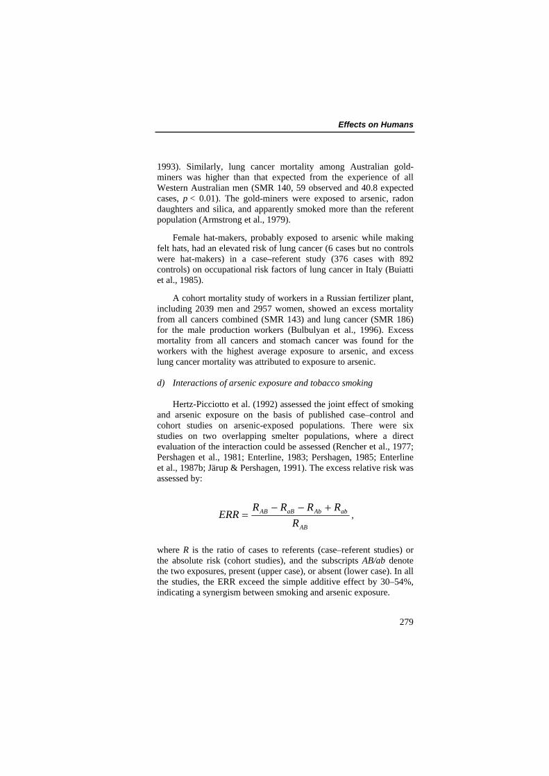
Effects on Humans 1993). Similarly, lung cancer mortality among Australian gold-miners was higher than that expected from the experience of all Western Australian men (SMR 140, 59 observed and 40.8 expected cases, p < 0.01). The gold-miners were exposed to arsenic, radon daughters and silica, and apparently smoked more than the referent population (Armstrong et al., 1979). Female hat-makers, probably exposed to arsenic while making felt hats, had an elevated risk of lung cancer (6 cases but no controls were hat-makers) in a case–referent study (376 cases with 892 controls) on occupational risk factors of lung cancer in Italy (Buiatti et al., 1985). A cohort mortality study of workers in a Russian fertilizer plant, including 2039 men and 2957 women, showed an excess mortality from all cancers combined (SMR 143) and lung cancer (SMR 186) for the male production workers (Bulbulyan et al., 1996). Excess mortality from all cancers and stomach cancer was found for the workers with the highest average exposure to arsenic, and excess lung cancer mortality was attributed to exposure to arsenic. d) Interactions of arsenic exposure and tobacco smoking Hertz-Picciotto et al. (1992) assessed the joint effect of smoking and arsenic exposure on the basis of published case–control and cohort studies on arsenic-exposed populations. There were six studies on two overlapping smelter populations, where a direct evaluation of the interaction could be assessed (Rencher et al., 1977; Pershagen et al., 1981; Enterline, 1983; Pershagen, 1985; Enterline et al., 1987b; Järup & Pershagen, 1991). The excess relative risk was assessed by:

AB

abAbaBAB

RRRRR

ERR+−−

= ,

where R is the ratio of cases to referents (case–referent studies) or the absolute risk (cohort studies), and the subscripts AB/ab denote the two exposures, present (upper case), or absent (lower case). In all the studies, the ERR exceed the simple additive effect by 30–54%, indicating a synergism between smoking and arsenic exposure.

279

EHC 224: Arsenic and Arsenic Compounds e) Lung cancer in the vicinity of arsenic-emitting industries Mortality rates for lung cancer for white men and women in 1950–1960 were significantly higher in US counties with copper, lead, or zinc smelting and refining industries (Blot & Fraumeni, 1975), and a 2-fold mortality of lung cancer was observed among people with residence near a zinc smelter, and in areas with high topsoil concentrations of arsenic, cadmium, copper, lead and manganese (Brown et al., 1984). A slightly higher mortality of lung cancer was observed among male residents of Rouyn-Noranda, a community with a copper smelter, than among male residents of a referent community (SMR 150) or Quebec (Canada) as a whole (SMR 120); no such difference was observed among women (only 7 exposed cases) (Cordier et al., 1983). Although the lung cancer mortality between 1935 and 1969 in women living in three geographically defined areas in the vicinity of an arsenic-emitting smelter was not different from that expected from nationwide expected figures, there was a positive trend following predicted exposure levels (Frost et al., 1987). No difference was observed between the frequency of lung cancer and that of other cancers in the vicinity of non-ferrous smelters (a lead-zinc smelter and 10 copper smelters) in the USA (Greaves et al., 1981). The lung cancer mortality among people living in the vicinity of a copper smelter in Rönnskär (Sweden) was studied in a cohort and a case–referent study (Pershagen et al., 1977; Pershagen, 1985). In the cohort study, a significantly higher mortality from lung cancer was observed among men living close to the smelter than among men in a reference area (Pershagen et al., 1977). The difference disappeared, however, when men working in the smelter were excluded. In the case–referent study, the odds ratio (OR) for residence in the exposed area was 2.0 (95% CI 1.2–3.4), and it was not explained by occupation in the smelter, or by differences in smoking habits (Pershagen, 1985). Lung cancer mortality was higher in men living in the vicinity of a factory producing arsenical pesticides in Baltimore (Maryland, USA) (Matanoski et al., 1981). No association between the distance from a smelter and lung cancer risk was observed in a case–referent study where 575 lung cancer cases were compared with 1490 breast and prostate cases collected from 1944 to 1973 in El Paso, Texas (USA), where a smelter had been operating since 1887 (Rom et al., 1982).

280

Effects on Humans In a study of lung cancer mortality in 6 Arizona (USA) copper smelter towns, using 185 lung cancer cases and 2 matched controls per case from decedent residents during 1979–1990, information on lifetime residential, occupational, and smoking history was obtained (Marsh et al., 1997, 1998). Historical environmental exposures to smelter emissions were linked with residential histories to derive individual profiles of residential exposure. Occupational histories were characterized by potential exposure to smelter emissions, asbestos and ionizing radiation. No statistically significant associ-ations were observed between lung cancer risk and residential exposure to smelter emissions, when adjustment for potential confounding factors (gender, Hispanic ethnicity, and smoking) were made. The authors concluded that the study provided little evidence of a positive association between lung cancer mortality and residential exposure to smelter emissions. A Chinese case–control study including 1249 lung cancer patients and 1345 population-based controls showed 3-fold elevated risks among smelter workers (Xu et al., 1989, 1991). Soil levels of arsenic rose with increasing proximity to the Shenyang copper smelter, and, after controlling for smoking and work experience in the smelter, elevated risks of lung cancer were found among men, but not women, living within 1 km of its central stacks. It has been noted that epidemiological studies designed to detect lung cancer risk and other health effects in communities surrounding arsenic-producing copper smelters usually have insufficient statistical power to detect the small increases in risk that may occur (Hughes et al., 1988). Most such studies have little power to detect relative risks under 2.0. The authors argue that these studies may be a good and economical first investigation but, because of the lack of statistical power, null findings do not rule out the possibility of excess risks that may be significant from a public health viewpoint. f) Exposure–response relationships Sufficient information on the levels of exposure to ensure reliable assessment of the exposure–response relationships can be found only in the three copper smelter cohorts: Tacoma, Anaconda and Rönnskär. In all, there was an increase in lung cancer risk with increasing exposure (Table 32, Fig. 4). The risk seems to increase

281

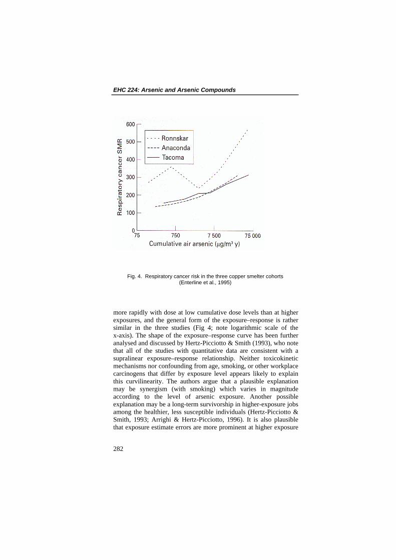
EHC 224: Arsenic and Arsenic Compounds

Fig. 4. Respiratory cancer risk in the three copper smelter cohorts (Enterline et al., 1995)

more rapidly with dose at low cumulative dose levels than at higher exposures, and the general form of the exposure–response is rather similar in the three studies (Fig 4; note logarithmic scale of the x-axis). The shape of the exposure–response curve has been further analysed and discussed by Hertz-Picciotto & Smith (1993), who note that all of the studies with quantitative data are consistent with a supralinear exposure–response relationship. Neither toxicokinetic mechanisms nor confounding from age, smoking, or other workplace carcinogens that differ by exposure level appears likely to explain this curvilinearity. The authors argue that a plausible explanation may be synergism (with smoking) which varies in magnitude according to the level of arsenic exposure. Another possible explanation may be a long-term survivorship in higher-exposure jobs among the healthier, less susceptible individuals (Hertz-Picciotto & Smith, 1993; Arrighi & Hertz-Picciotto, 1996). It is also plausible that exposure estimate errors are more prominent at higher exposure

282

Effects on Humans levels as a result of past industrial hygiene sampling or worker protection practices (Hertz-Picciotto & Smith, 1993), which is consistent with the findings of the sensitivity analysis of the Rönnskär data (Järup, 1992), and the update of the Anaconda cohort (Lubin et al., 2000). Analyses performed on a subcohort at the Tacoma smelter suggested that there was strong evidence of confounding by year of initial hire, with a non-linear exposure–response evident only among workers hired before 1940 (Viren & Silvers, 1999). Among workers hired after 1940, analyses showed that a linear dose–response provided a clearly superior fit. Re-analysis of the Anaconda cohort (Lubin et al., 2000) is also in favour of a linear exposure-risk relationship, and ascribes the apparent non-linearity to overestimation of the high exposures (mainly because of use of protective devices). 32. All three main studies demonstrate a statistically significant excess risk of lung cancer at exposure levels of approximately ≥0.75 (mg/m3) ⋅ year.

8.7.1.2 Cancer at other sites (Table 32) 34. Autopsy series (Roth, 1955, 1957a,b) on wine growers (exposure from wine consumption and arsenical pesticide application) have linked arsenic exposure to hepatic angiosarcoma. Among 168 people diagnosed with hepatic angiosarcoma in the USA, occupational exposure to arsenic was found in 4 cases and exposure to Fowler’s solution in 6 (Falk et al., 1981a,b); among 43 cases diagnosed in the state of New York between 1958 and 1979, 6 had a possible history of occupational exposure to arsenic (Vianna et al., 1981). Although statistically not significant, arsenic exposure was associated with an increased risk of kidney cancer in the Tacoma cohort (SMR 164, 11 observed and 6.73 expected cases) (Enterline et al., 1995) (Table 32). The kidney cancer was not in excess in the, 1938–1987 follow-up of the Anaconda cohort (SMR 57, CI 33–101) (Lubin et al., 2000). No cases of kidney cancer (1.48 expected) were observed in a French gold-miner cohort (Simonato et al., 1994) or in

283

EHC 224: Arsenic and Arsenic Compounds the US pesticide-producer cohort (1.8 expected) (Sobel et al., 1988). No significant relationship was observed between arsenic exposure and incidence of cancer in 1958–1982 of the large “urogenital organs” category in the Swedish cohort (Sandström et al., 1989). Hill & Faning (1948) found a remarkably elevated relative skin cancer mortality among workers in a sheep-dip factory manu-facturing sodium arsenite. Among 47 autopsies of winegrowers with arsenic intoxication (exposure from wine consumption and arsenical pesticide application), 13 of the subjects had a total of 40 skin cancers (Roth, 1958). A case series on skin cancer among arsenic-exposed wine growers has been published (Thiers et al., 1967). No excess skin cancer was observed in the Anaconda cohort (SMR 53, CI 26–106) (Lubin et al, 2000). Wong et al. (1992) compared skin cancer incidence in two counties in Montana (USA) considered potentially exposed to arsenic and two counties in the same state considered not exposed, during the period 1 January 1980 to 30 June 1986. Arsenic exposure in the counties potentially exposed to arsenic would have occurred through inhalation or ingestion of arsenic-contaminated soil and or dust resulting from the presence of an open-pit copper mine in Butte, and a copper smelter at Anaconda. Skin cancer cases were identified from surgical and biopsy specimen reports from pathologists’ and hospital records and dermatologists’ office records. Age-, race- and sex-specific population data for the four counties were obtained from the US Census Bureau (1980 census). The age-adjusted annual skin cancer rates were found to be higher in the control counties than in the two exposed counties. No evidence is provided by the authors as to how much arsenic exposure may have been experienced by the residents of the counties where there was “potential exposure”, considerably limiting the interpretation of the study’s results. Significant relationship was observed between arsenic exposure and incidence of cancer in 1958–1982 in the large “digestive organs” category in the Swedish smelter cohort (Sandström et al., 1989). No increase in the risk of cancer of digestive organs and peritoneum was observed in the Anaconda cohort (SMR 94, CI 83–107) (Lubin et al, 2000). No excess of stomach cancer was observed in the Japanese smelter cohort (SMR 68, 10 observed and 14.71 expected cases

284

Effects on Humans (Tokudome & Kuratsune, 1976). The SMR for stomach cancer was 116 (CI 91–149) in the Anaconda smelter cohort (Lubin et al., 2000). There was an increase in the cancer of the large intestine (SMR 162, 38 observed and 23.48 expected cases, p < 0.01) in the Tacoma smelter cohort (Enterline et al., 1995). There was similarly a moderate excess of rectal cancer (SMR 176, 15 observed and 8.52 expected cases, NS) in the Tacoma cohort (Enterline et al., 1995), and in the French gold-miner cohort (SMR 280, 95% CI 113–577) (Simonato et al., 1994). Although statistically non-significant, arsenic exposure was associated with an increased risk of cancer of the buccal cavity and pharynx in the Tacoma refinery cohort (SMR 169, 12 observed and 7.12 expected cases) (Enterline et al., 1995), but no such excess was observed in the Anaconda smelter cohort in 1964–1977 (SMR 97, CI 66–143) (Lubin et al., 2000) or in the US pesticide producer cohort (0 observed, 1.5 expected) (Sobel et al., 1988). There was an association of arsenic exposure with cancer of the bone in the Tacoma smelter cohort (SMR 456, 5 observed and 1.10 expected cases; two of the cases apparently were not primary bone tumours) (Enterline et al., 1995).

8.7.2 Exposure via drinking-water (Table 33) The first ecological study by Chen et al. (1985) investigated the cancer mortality in 84 communities in four townships (Peimen, Hsuechia, Putai, and Ichu) on south-western coast of Taiwan in, 1968–82, and compared the age-adjusted rates to figures of all Taiwan. During the study period, the population of Taiwan increased by ~35%, whereas that in the BFD-endemic area decreased by ~15%, mainly because of emigration. As it is mandatory to register each death using a standardized death certificate, the authors state that the statistics are “very complete”. They also report that 85% of all cancer deaths except liver cancer deaths are confirmed by histological or cytological analysis. The mortality (SMR) from lung, liver, kidney, bladder and skin cancers was substantially elevated in the BFD-endemic area; there

285

EHC 224: Arsenic and Arsenic Compounds was a moderate excess in the mortality from colon cancer, and no excess in the mortality from nasopharyngeal, oesophageal, stomach, small-intestinal or rectal cancer, or leukaemia (Chen et al., 1985). Chen et al. (1986) also carried out a case–referent study on cancer in this population. Cases were people who died of bladder, lung or liver cancer, confirmed diagnostically either by biopsy or by other tests. Controls were selected from the same geographical areas as the cases, frequency-matched on age and sex. Structured questionnaires included history of artesian water use, socio-demographic variables, dietary and lifestyle habits, as well as medical history. Proxy interviews of relatives were used for deceased cases. The total number of bladder, lung and liver cancer cases were 70, 77 and 65, respectively (response rates of 93%, 90% and 93%), with the same controls used for all the cases (n = 368, 92% response rate). The ORs of liver, lung and bladder cancer cases showed an increasing risk with increasing duration of exposure (see Table 33). The trend remained significant for the cancers of lung and bladder after controlling for age, sex, cigarette smoking, tea drinking, vegetarian habit, vegetable consumption frequency and consumption of fermented beans. Chen et al. (1988b) followed the vital status of a cohort of 871 BFD patients from 1968 to 1984; 84 (9.6%) were lost to follow-up, for 8 the cause of death was ill-defined and for 6 there was an undefined cancer on the death certificate. The cause-specific mortality was compared to that of the whole of Taiwan, and to that of the BFD-endemic area. The SMR of cancer of the lung, liver, kidney, bladder and skin was markedly elevated among BFD patients in comparison to the Taiwanese population, and somewhat less in comparison to the population in the endemic area without BFD. An excess (SMR 381, 4 cases, p < 0.05) of colon cancer was observed in comparison to the national figures; which was not significant in comparison to referents from the BFD-endemic area. The SMR from stomach cancer was not significantly elevated (Chen et al., 1988b). A further ecological study in south-western Taiwan (Wu et al., 1989) investigated the mortality in 1973–1986 from vascular diseases and cancer of residents in 42 villages in Peimen, Hsuechia,

286

Effects on Humans Putai, Yensui and Hsiyang townships, where data on well-water arsenic concentrations had been measured in the early 1960s. This study covers 27 of the 84 townships studied in the first study, with the addition of two other townships, Yensui and Hsiyang. The overlap of this study with the first study cannot be fully assessed. The villages were classified into three categories on the basis of the median well-water arsenic concentrations: < 300 µg/litre, 300-590 µg/litre, and > 600 µg/litre, as determined in the 1964–1966 survey. Death certificates were used to ascertain cause of death, and person-years for the same time period were calculated on the basis of demographic reports. A further exposure–response analysis from these data is presented in a further study (Chen et al., 1992), where the lowest exposure category is divided into two (< 100 and 100-300 µg/litre). Although the follow-up time and the overall person-years of follow-up for these two analyses were identical, the numbers of deaths were larger for all sites in the later analysis: 304 vs. 268 for lung cancer, 202 vs. 174 for liver cancer, 202 vs. 181 for bladder cancer and 64 vs. 59 for kidney cancer. Furthermore, a preliminary report of the same study (Chen et al., 1988a) gives still another (lowest) risk estimate for all cancer sites (based on 1031 cancer deaths, compared to 1152 in the study by Wu et al., 1989). The age-adjusted mortality rates from lung, liver, kidney and bladder cancer, as well as those from skin cancer, showed an association with the village median well-water arsenic concentration in both men and women. Where the number of cases allowed a meaningful interpretation, the monotonic exposure–response relationship continued at the lower exposure levels studied (< 100 and 100–300 µg/litre) in the later report (Chen et al., 1992). No significant association was observed for cancers of the nasopharynx, oesophagus, stomach, colon or uterine cervix, or leukaemia (Wu et al., 1989). Chen & Wang (1990) performed a further ecological study on drinking-water arsenic concentration and mortality from malignant neoplasms in 1972–1983, where the unit of study was all 314 precincts and townships in Taiwan where the well arsenic concentration had been analysed in 1974–1976. Nearly all cancer deaths among the arsenic exposed in this study seem to be included in the study by Chen et al. (1985). The average precinct or township well-water arsenic concentration was taken as the indicator of

287

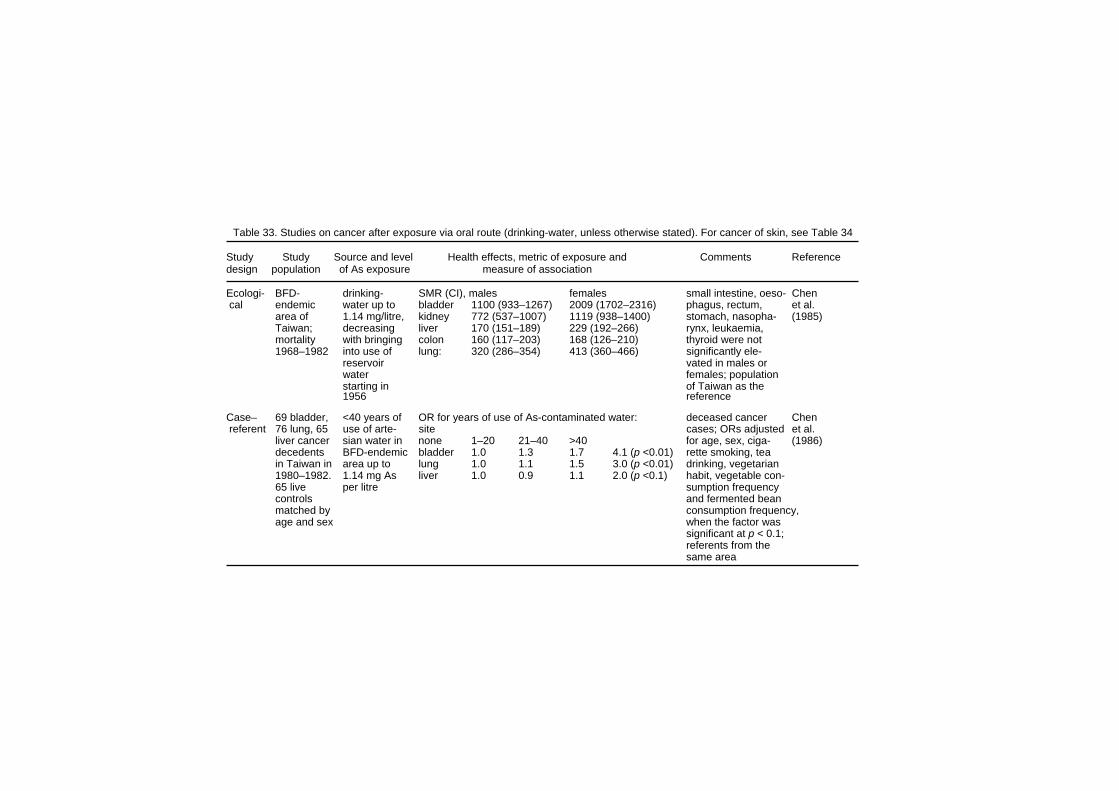
Table 33. Studies on cancer after exposure via oral route (drinking-water, unless otherwise stated). For cancer of skin, see Table 34 Study Study Source and level Health effects, metric of exposure and Comments Reference design population of As exposure measure of association Ecologi- BFD- drinking- SMR (CI), males females small intestine, oeso- Chen cal endemic water up to bladder 1100 (933–1267) 2009 (1702–2316) phagus, rectum, et al. area of 1.14 mg/litre, kidney 772 (537–1007) 1119 (938–1400) stomach, nasopha- (1985) Taiwan; decreasing liver 170 (151–189) 229 (192–266) rynx, leukaemia, mortality with bringing colon 160 (117–203) 168 (126–210) thyroid were not 1968–1982 into use of lung: 320 (286–354) 413 (360–466) significantly ele- reservoir vated in males or water females; population starting in of Taiwan as the 1956 reference Case– 69 bladder, <40 years of OR for years of use of As-contaminated water: deceased cancer Chen referent 76 lung, 65 use of arte- site cases; ORs adjusted et al. liver cancer sian water in none 1–20 21–40 >40 for age, sex, ciga- (1986) decedents BFD-endemic bladder 1.0 1.3 1.7 4.1 (p <0.01) rette smoking, tea in Taiwan in area up to lung 1.0 1.1 1.5 3.0 (p <0.01) drinking, vegetarian 1980–1982. 1.14 mg As liver 1.0 0.9 1.1 2.0 (p <0.1) habit, vegetable con- 65 live per litre sumption frequency controls and fermented bean matched by consumption frequency, age and sex when the factor was significant at p < 0.1; referents from the same area

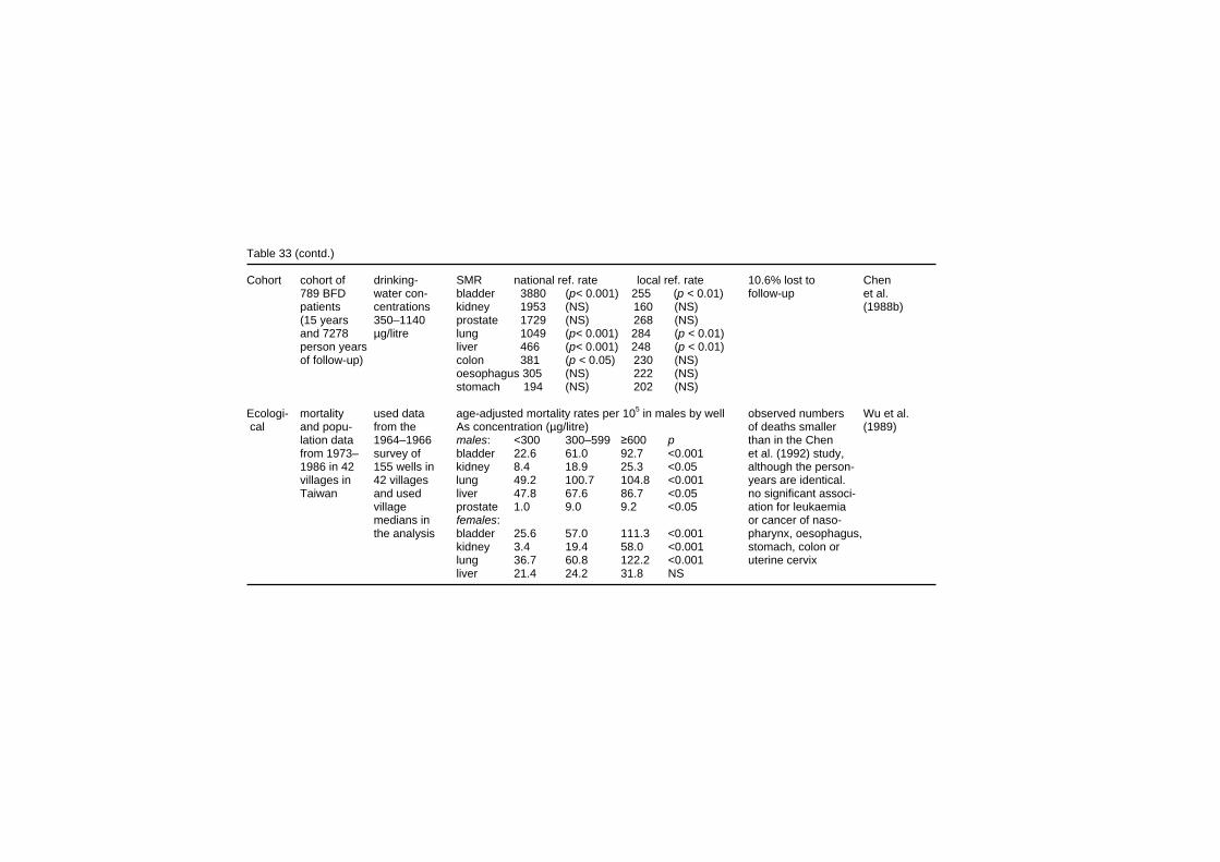
Table 33 (contd.) Cohort cohort of drinking- SMR national ref. rate local ref. rate 10.6% lost to Chen 789 BFD water con- bladder 3880 (p< 0.001) 255 (p < 0.01) follow-up et al. patients centrations kidney 1953 (NS) 160 (NS) (1988b) (15 years 350–1140 prostate 1729 (NS) 268 (NS) and 7278 µg/litre lung 1049 (p< 0.001) 284 (p < 0.01) person years liver 466 (p< 0.001) 248 (p < 0.01) of follow-up) colon 381 (p < 0.05) 230 (NS) oesophagus 305 (NS) 222 (NS) stomach 194 (NS) 202 (NS) Ecologi- mortality used data age-adjusted mortality rates per 105 in males by well observed numbers Wu et al. cal and popu- from the As concentration (µg/litre) of deaths smaller (1989) lation data 1964–1966 males: <300 300–599 ≥600 p than in the Chen from 1973– survey of bladder 22.6 61.0 92.7 <0.001 et al. (1992) study, 1986 in 42 155 wells in kidney 8.4 18.9 25.3 <0.05 although the person- villages in 42 villages lung 49.2 100.7 104.8 <0.001 years are identical. Taiwan and used liver 47.8 67.6 86.7 <0.05 no significant associ- village prostate 1.0 9.0 9.2 <0.05 ation for leukaemia medians in females: or cancer of naso- the analysis bladder 25.6 57.0 111.3 <0.001 pharynx, oesophagus, kidney 3.4 19.4 58.0 <0.001 stomach, colon or lung 36.7 60.8 122.2 <0.001 uterine cervix liver 21.4 24.2 31.8 NS

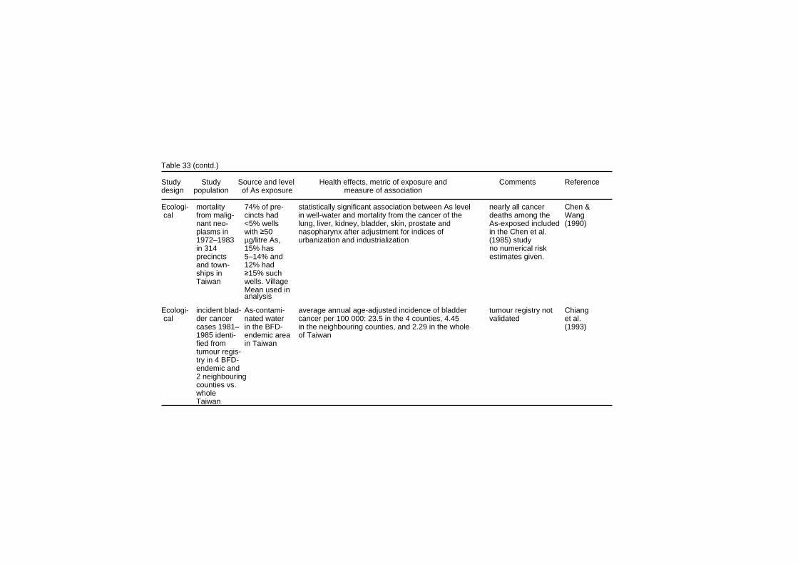
Table 33 (contd.) Study Study Source and level Health effects, metric of exposure and Comments Reference design population of As exposure measure of association Ecologi- mortality 74% of pre- statistically significant association between As level nearly all cancer Chen & cal from malig- cincts had in well-water and mortality from the cancer of the deaths among the Wang nant neo- <5% wells lung, liver, kidney, bladder, skin, prostate and As-exposed included (1990) plasms in with ≥50 nasopharynx after adjustment for indices of in the Chen et al. 1972–1983 µg/litre As, urbanization and industrialization (1985) study in 314 15% has no numerical risk precincts 5–14% and estimates given. and town- 12% had ships in ≥15% such Taiwan wells. Village Mean used in analysis Ecologi- incident blad- As-contami- average annual age-adjusted incidence of bladder tumour registry not Chiang cal der cancer nated water cancer per 100 000: 23.5 in the 4 counties, 4.45 validated et al. cases 1981– in the BFD- in the neighbouring counties, and 2.29 in the whole (1993) 1985 identi- endemic area of Taiwan fied from in Taiwan tumour regis- try in 4 BFD- endemic and 2 neighbouring counties vs. whole Taiwan

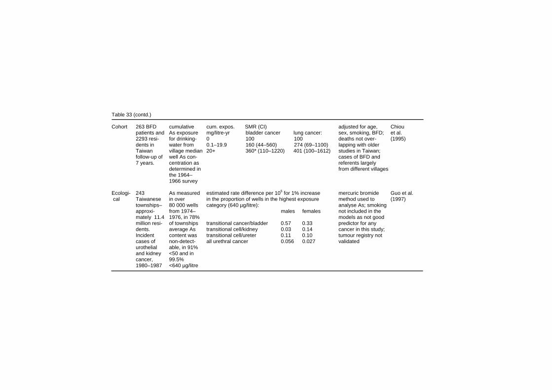
Table 33 (contd.) Cohort 263 BFD cumulative cum. expos. SMR (CI) adjusted for age, Chiou patients and As exposure mg/litre-yr bladder cancer lung cancer: sex, smoking, BFD; et al. 2293 resi- for drinking- 0 100 100 deaths not over- (1995) dents in water from 0.1–19.9 160 (44–560) 274 (69–1100) lapping with older Taiwan village median 20+ 360* (110–1220) 401 (100–1612) studies in Taiwan; follow-up of well As con- cases of BFD and 7 years. centration as referents largely determined in from different villages the 1964– 1966 survey Ecologi- 243 As measured estimated rate difference per 105 for 1% increase mercuric bromide Guo et al. cal Taiwanese in over in the proportion of wells in the highest exposure method used to (1997) townships– 80 000 wells category (640 µg/litre): analyse As; smoking approxi- from 1974– males females not included in the mately 11.4 1976, in 78% models as not good million resi- of townships transitional cancer/bladder 0.57 0.33 predictor for any dents. average As transitional cell/kidney 0.03 0.14 cancer in this study; Incident content was transitional cell/ureter 0.11 0.10 tumour registry not cases of non-detect- all urethral cancer 0.056 0.027 validated urothelial able, in 91% and kidney <50 and in cancer, 99.5% 1980–1987 <640 µg/litre

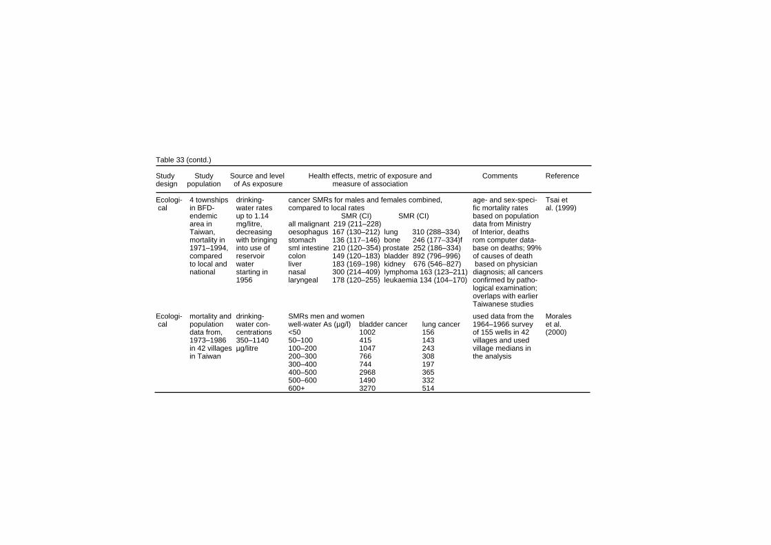
Table 33 (contd.) Study Study Source and level Health effects, metric of exposure and Comments Reference design population of As exposure measure of association Ecologi- 4 townships drinking- cancer SMRs for males and females combined, age- and sex-speci- Tsai et cal in BFD- water rates compared to local rates fic mortality rates al. (1999) endemic up to 1.14 SMR (CI) SMR (CI) based on population area in mg/litre, all malignant 219 (211–228) data from Ministry Taiwan, decreasing oesophagus 167 (130–212) lung 310 (288–334) of Interior, deaths mortality in with bringing stomach 136 (117–146) bone 246 (177–334)f rom computer data- 1971–1994, into use of sml intestine 210 (120–354) prostate 252 (186–334) base on deaths; 99% compared reservoir colon 149 (120–183) bladder 892 (796–996) of causes of death to local and water liver 183 (169–198) kidney 676 (546–827) based on physician national starting in nasal 300 (214–409) lymphoma 163 (123–211) diagnosis; all cancers 1956 laryngeal 178 (120–255) leukaemia 134 (104–170) confirmed by patho- logical examination; overlaps with earlier Taiwanese studies Ecologi- mortality and drinking- SMRs men and women used data from the Morales cal population water con- well-water As (µg/l) bladder cancer lung cancer 1964–1966 survey et al. data from, centrations <50 1002 156 of 155 wells in 42 (2000) 1973–1986 350–1140 50–100 415 143 villages and used in 42 villages µg/litre 100–200 1047 243 village medians in in Taiwan 200–300 766 308 the analysis 300–400 744 197 400–500 2968 365 500–600 1490 332 600+ 3270 514

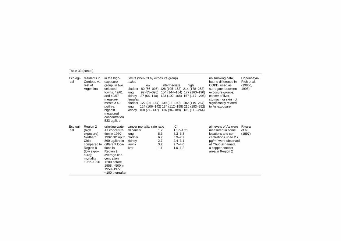
Table 33 (contd.) Ecologi- residents in in the high- SMRs (95% CI by exposure group) no smoking data, Hopenhayn- cal Cordoba vs. exposure males but no difference in Rich et al. rest of group, in two low intermediate high COPD, used as (1996c, Argentina selected bladder 80 (66–096) 128 (105–153) 214 (178–253) surrogate, between 1998) towns, 42/61 lung 92 (85–098) 154 (144–164) 177 (163–190) exposure groups; and 49/57 kidney 87 (66–110) 133 (102–168) 157 (117– 205) cancer of liver, measure- females stomach or skin not ments ≥ 40 bladder 122 (86–167) 139 (93–199) 182 (119–264) significantly related µg/litre; lung 124 (106–142) 134 (112–158) 216 (183–252) to As exposure highest kidney 100 (71–137) 136 (94–189) 181 (119–264) measured concentration 533 µg/litre Ecologi- Region 2 drinking-water cancer mortality rate ratio CI air levels of As were Rivara cal (high As concentra- all cancer 1.2 1.17–1.21 measured in some et al. exposure) tion in 1950– lung 5.6 5.3–6.3 locations and con- (1997) Northern 1992 ND up to bladder 6.7 5.9–7.7 centrations up to 2.7 Chile 860 µg/litre in kidney 2.7 2.4–3.1 µg/m3 were observed compared to different loca- larynx 3.2 2.7–4.0 at Chuquichamata, Region 8 tions in liver 1.1 1.0–1.2 a copper smelter (low expo- Region 2; area in Region 2 sure); average con- mortality centration 1952–1990 <200 before 1958, >500 in 1959–1977, <100 thereafter

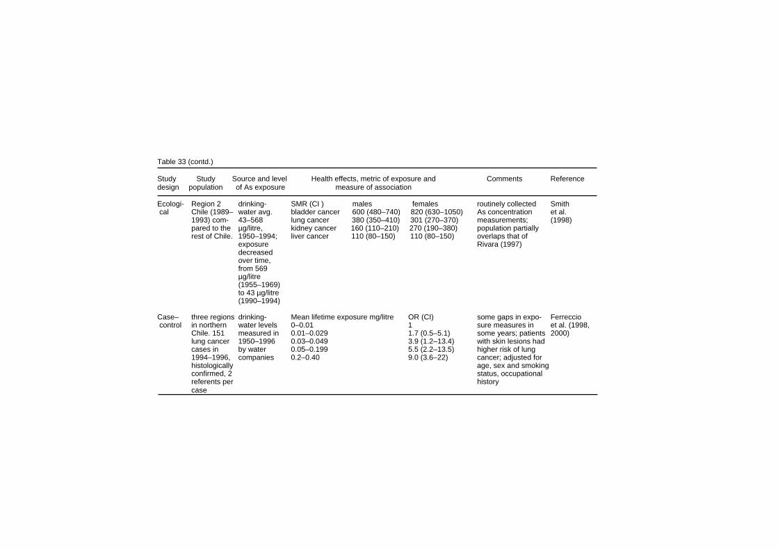
Table 33 (contd.) Study Study Source and level Health effects, metric of exposure and Comments Reference design population of As exposure measure of association Ecologi- Region 2 drinking- SMR (CI ) males females routinely collected Smith cal Chile (1989– water avg. bladder cancer 600 (480–740) 820 (630–1050) As concentration et al. 1993) com- 43–568 lung cancer 380 (350–410) 301 (270–370) measurements; (1998) pared to the µg/litre, kidney cancer 160 (110–210) 270 (190–380) population partially rest of Chile. 1950–1994; liver cancer 110 (80–150) 110 (80–150) overlaps that of exposure Rivara (1997) decreased over time, from 569 µg/litre (1955–1969) to 43 µg/litre (1990–1994) Case– three regions drinking- Mean lifetime exposure mg/litre OR (CI) some gaps in expo- Ferreccio control in northern water levels 0–0.01 1 sure measures in et al. (1998, Chile. 151 measured in 0.01–0.029 1.7 (0.5–5.1) some years; patients 2000) lung cancer 1950–1996 0.03–0.049 3.9 (1.2–13.4) with skin lesions had cases in by water 0.05–0.199 5.5 (2.2–13.5) higher risk of lung 1994–1996, companies 0.2–0.40 9.0 (3.6–22) cancer; adjusted for histologically age, sex and smoking confirmed, 2 status, occupational referents per history case

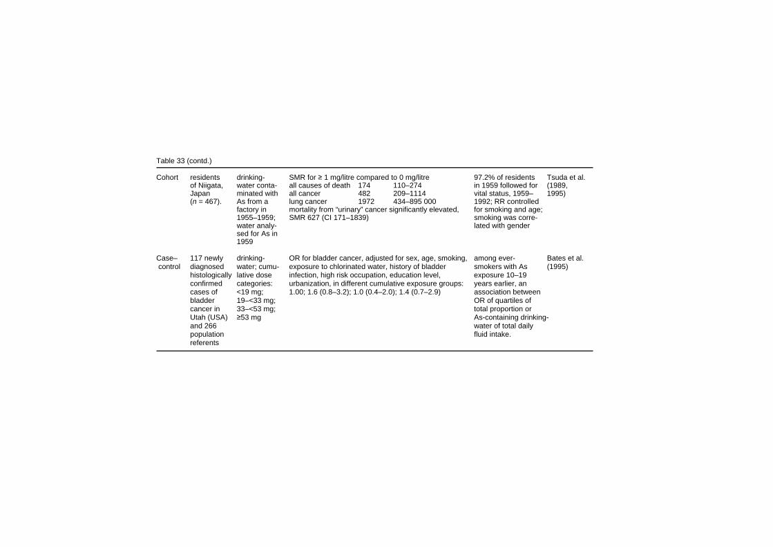
Table 33 (contd.) Cohort residents drinking- SMR for ≥ 1 mg/litre compared to 0 mg/litre 97.2% of residents Tsuda et al. of Niigata, water conta- all causes of death 174 110–274 in 1959 followed for (1989, Japan minated with all cancer 482 209–1114 vital status, 1959– 1995) (n = 467). As from a lung cancer 1972 434–895 000 1992; RR controlled factory in mortality from “urinary” cancer significantly elevated, for smoking and age; 1955–1959; SMR 627 (CI 171–1839) smoking was corre- water analy- lated with gender sed for As in 1959 Case– 117 newly drinking- OR for bladder cancer, adjusted for sex, age, smoking, among ever- Bates et al. control diagnosed water; cumu- exposure to chlorinated water, history of bladder smokers with As (1995) histologically lative dose infection, high risk occupation, education level, exposure 10–19 confirmed categories: urbanization, in different cumulative exposure groups: years earlier, an cases of <19 mg; 1.00; 1.6 (0.8–3.2); 1.0 (0.4–2.0); 1.4 (0.7–2.9) association between bladder 19–<33 mg; OR of quartiles of cancer in 33–<53 mg; total proportion or Utah (USA) ≥53 mg As-containing drinking- and 266 water of total daily population fluid intake. referents

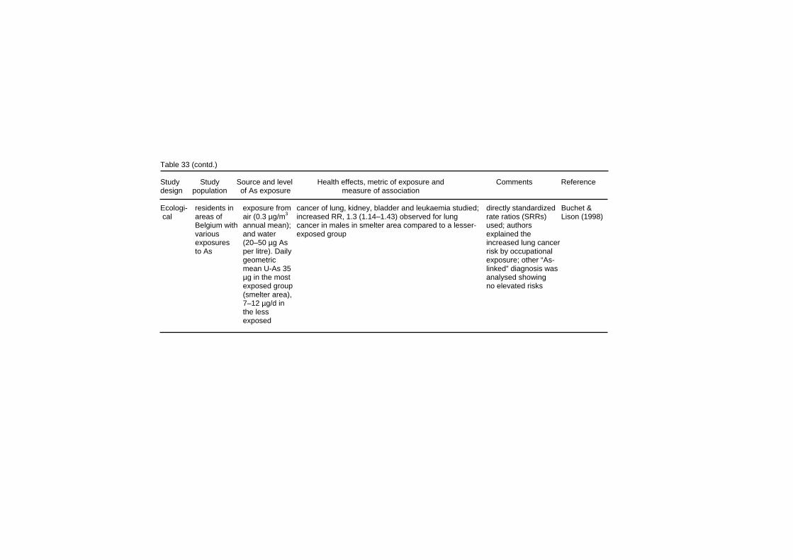
Table 33 (contd.) Study Study Source and level Health effects, metric of exposure and Comments Reference design population of As exposure measure of association Ecologi- residents in exposure from cancer of lung, kidney, bladder and leukaemia studied; directly standardized Buchet & cal areas of air (0.3 µg/m3 increased RR, 1.3 (1.14–1.43) observed for lung rate ratios (SRRs) Lison (1998) Belgium with annual mean); cancer in males in smelter area compared to a lesser- used; authors various and water exposed group explained the exposures (20–50 µg As increased lung cancer to As per litre). Daily risk by occupational geometric exposure; other “As- mean U-As 35 linked” diagnosis was µg in the most analysed showing exposed group no elevated risks (smelter area), 7–12 µg/d in the less exposed

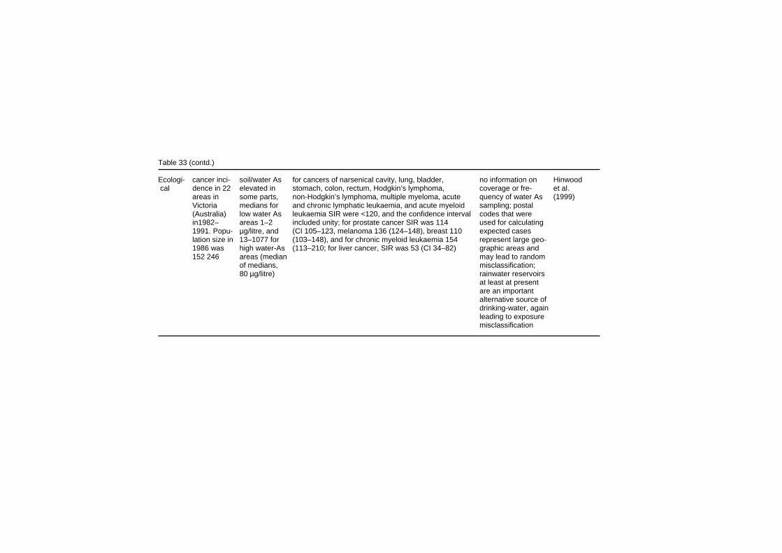
Table 33 (contd.) Ecologi- cancer inci- soil/water As for cancers of narsenical cavity, lung, bladder, no information on Hinwood cal dence in 22 elevated in stomach, colon, rectum, Hodgkin’s lymphoma, coverage or fre- et al. areas in some parts, non-Hodgkin’s lymphoma, multiple myeloma, acute quency of water As (1999) Victoria medians for and chronic lymphatic leukaemia, and acute myeloid sampling; postal (Australia) low water As leukaemia SIR were <120, and the confidence interval codes that were in1982– areas 1–2 included unity; for prostate cancer SIR was 114 used for calculating 1991. Popu- µg/litre, and (CI 105–123, melanoma 136 (124–148), breast 110 expected cases lation size in 13–1077 for (103–148), and for chronic myeloid leukaemia 154 represent large geo- 1986 was high water-As (113–210; for liver cancer, SIR was 53 (CI 34–82) graphic areas and 152 246 areas (median may lead to random of medians, misclassification; 80 µg/litre) rainwater reservoirs at least at present are an important alternative source of drinking-water, again leading to exposure misclassification

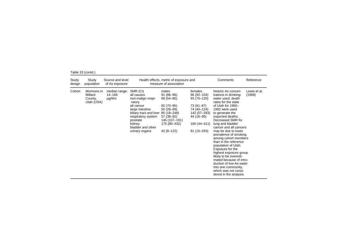
Table 33 (contd.) Study Study Source and level Health effects, metric of exposure and Comments Reference design population of As exposure measure of association Cohort Mormons in median range: SMR (CI) males females historic As concen- Lewis et al. Millard 14–166 all causes 91 (86–96) 96 (92–104) trations in drinking- (1999) County, µg/litre non-malign respi- 68 (54–85) 93 (70–120) water used; death Utah (USA) ratory rates for the state all cancer 82 (70–95) 73 (61–87) of Utah for 1960– large intestine 50 (28–99) 74 (40–124) 1992 were used biliary tract and liver 85 (18–248) 142 (57–293) to generate the respiratory system 57 (38–82) 44 (16–95) expected deaths. prostate 145 (107–191) Decreased SMR for kidney 175 (80–332) 160 (44–411) lung and bladder bladder and other cancer and all cancers urinary organs 42 (8–122) 81 (10–293) may be due to lower prevalence of smoking among cohort members than in the reference population of Utah. Exposure for the highest exposure group likely to be overesti- mated because of intro- duction of low-As water into one community, which was not consi- dered in the analysis

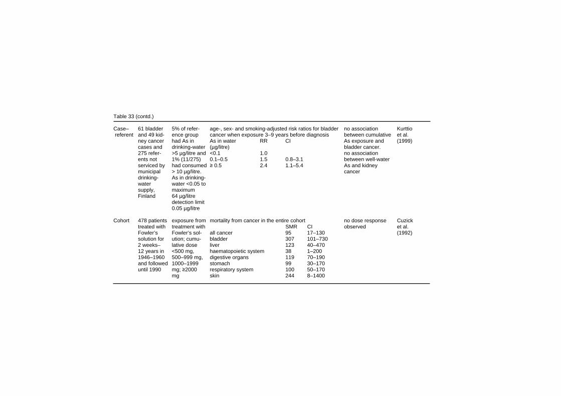
Table 33 (contd.) Case– 61 bladder 5% of refer- age-, sex- and smoking-adjusted risk ratios for bladder no association Kurttio referent and 49 kid- ence group cancer when exposure 3–9 years before diagnosis between cumulative et al. ney cancer had As in As in water RR CI As exposure and (1999) cases and drinking-water (µg/litre) bladder cancer. 275 refer- >5 µg/litre and <0.1 1.0 no association ents not 1% (11/275) 0.1–0.5 1.5 0.8–3.1 between well-water serviced by had consumed ≥ 0.5 2.4 1.1–5.4 As and kidney municipal > 10 µg/litre. cancer drinking- As in drinking- water water <0.05 to supply, maximum Finland 64 µg/litre detection limit 0.05 µg/litre Cohort 478 patients exposure from mortality from cancer in the entire cohort no dose response Cuzick treated with treatment with SMR CI observed et al. Fowler’s Fowler’s sol- all cancer 95 17–130 (1992) solution for ution; cumu- bladder 307 101–730 2 weeks– lative dose liver 123 40–470 12 years in <500 mg, haematopoietic system 38 1–200 1946–1960 500–999 mg, digestive organs 119 70–190 and followed 1000–1999 stomach 99 30–170 until 1990 mg; ≥2000 respiratory system 100 50–170 mg skin 244 8–1400

EHC 224: Arsenic and Arsenic Compounds arsenic exposure (continuous variable), and the information concerning death numbers and causes of death, as well as midyear population by age, sex, calendar year and precinct, were obtained from the Taiwan provincial department of health. The relationship between arsenic exposure, and mortality from cancer at 21 sites was analysed using multiple linear regression, adjusting for urbanization and industrialization of the precinct or township. Multivariate analysis, adjusting for indices of urbanization and industrialization, revealed a statistically significant association between arsenic level in well-water and mortality from cancer of the lung, liver, kidney, bladder, skin, prostate and nasopharynx. Mortality from liver cancer was three times higher for men than for women (Chen & Wang, 1990). In a cancer registry study in Taiwan, incident cases of bladder cancer in 1981–1985 were identified from the National Cancer Registration Centre, and the population was estimated from yearly registration in four counties endemic for BFD (Putai, Peimen, Hsuehchia, Yihjwu) The average annual age-adjusted incidence of bladder cancer in the four counties was 23.5 × 10–5; in the whole of Taiwan it was 2.29 × 10–5 (Chiang et al., 1993). In two neighbouring counties (Jiangjiun and Yanshoei), also considered to be endemic for BFD, the annual incidence of bladder cancer was 4.45 × 10–5. The computerized tumour registry began in 1982, and the registry was not validated. Chiou et al. (1995) studied cancer incidence during a 7-year period in the BFD-endemic area in south-western Taiwan among 263 people with BFD and 2293 healthy controls from the area. Their cancer incidence was monitored from annual health examinations, home visits, household registration, national death certification and the national cancer registry. This study apparently represents a population independent of the earlier Taiwanese studies, since deaths from 1986 to 1993 were analysed. It should be noted that during the follow-up 7 of the healthy controls were diagnosed with BFD, and that 257/263 of the cases, but only 753/2293 referents, were identified in the earlier study (Chen et al., 1988b) from the townships of Peimen, Hsuechia, Putai, or Ichu, the rest coming from three further villages and identified later, in 1988. The prevalence of BFD was 5.57, 3.87, 2.02, and 0.64/1000 for the different townships in the

300

Effects on Humans first population, but 9.6–13.6/1000 in the latter. History of residence, use of artesian well-water for drinking, tobacco-smoking habits and other possible confounding factors were analysed from question-naires. The personal arsenic exposure was assessed from residence history, use of artesian well-water, and median village well-water arsenic concentrations defined in the survey in the 1960s (see above). Age, status of BFD (diseased or not), the concentration of arsenic in drinking-water, the duration of drinking artesian well-water, and estimated cumulative arsenic exposure of drinking artesian well-water (measured in (mg/litre) ⋅ year), were statistically significantly related to the risk of lung and bladder cancer risk in a multivariate analysis. In addition, tobacco smoking was related to risk of lung cancer, but not bladder cancer. In an ecological study on bladder cancer incidence in 243 townships with (previous) high drinking-water arsenic concentration (Guo et al., 1997), the number of wells with a specified arsenic concentration (from the survey in 1974–1976 using the standard mercury bromide method, see above) was studied as a determinant of bladder cancer incidence in 1980–1987. A small part of the original Chen et al. (1985) study population, and an unknown large part of the population in the Wu et al. (1989) study, are included in this study. The percentage of wells in the highest arsenic-exposure category (of six categories, > 640 µg/litre) was significantly related to the incidence of transitional cell carcinoma of the bladder, ureter, urethra and kidney, and of adenocarcinoma of the bladder, but not to squamous cell carcinoma of the bladder, or of renal cell carcinoma, or of nephroblastoma. The tumour registry was not validated. Age-adjusted mortality rate ratios for cancer of lung, liver, bladder and skin combined were studied in 3-year time periods in four townships in the BFD-endemic area in Taiwan from 1971 to 1994, when there apparently was a time-dependent decrease in the drinking-water concentration of arsenic. A gradual decrease in the risk was observed in men over 40 years of age, but for men less than 40 years of age little change was observed; for women both over and under 40 years, the risks were lowest during the last two 3-year periods studied (Tsai et al., 1998). In the update of the ecological study (Chen et al., 1985) in Taiwan (Tsai et al., 1999), statistically significantly elevated

301

EHC 224: Arsenic and Arsenic Compounds mortalities were observed from cancer of the lung, larynx, oesophagus, stomach, small intestine, colon, rectum, liver, nose, larynx, lung, bone, prostate, bladder, kidney and skin, as well as from lymphoma and leukaemia. Mortality from nasopharyngeal, buccal or pharyngeal cancer was not elevated. The arsenic exposure–response relationships for lung, bladder, and liver cancer were recently modelled using data from the BFD-endemic area (Morales et al. 2000). Exposure groupings were based on individual well-water arsenic concentrations for each village. Depending on the model and whether or not a comparison population was used in the analysis, risk estimates varied widely (many by at least an order of magnitude). Independent of the modelling, the authors reported excess lung and bladder cancer risks at exposure concentrations < 50 µg/litre (see Table 33). The relationship between drinking-water arsenic and mortality from cancers at several sites in 26 rural counties in Córdoba (Argentina) in 1986–1991 was the subject of an ecological study (Hopenhayn-Rich et al., 1996c, 1998). Mortality rates in this area were compared with expected figures based on 1991 data for the whole of Argentina. The counties were divided into three drinking-water arsenic strata on the basis of a limited number of measurements and the relative number of reports on arsenical skin diseases. In two counties in the high-exposure group, 42/61 and 49/57 measurements were above the detection limit (40 µg/litre); the highest measured concentration was 533 µg/litre and the average drinking-water concentration of the measurements above 40 µg/litre in the two “high-exposure” counties was 178 µg/litre; the authors note, however, that this should not be considered to be representative of the population exposure (Hopenhayn-Rich et al., 1996d). To control for the potential confounding effect of smoking, mortality from chronic obstructive pulmonary disease was also assessed. The mortality from lung, kidney and bladder cancer was lowest in the counties with presumed lowest drinking-water arsenic concentration, intermediate in the medium exposure counties, and high in the high-exposure counties. The relative risk of chronic obstructive pulmonary disease was below unity for most groups and if anything, inversely related to arsenic exposure. The mortality from stomach, liver or skin cancer showed no clear-cut relationship with presumed arsenic exposure.

302

Effects on Humans In an ecological study on arsenic exposure and cancer in Chile, mortality in Region II during 1950–1992 was compared to the more southerly Region VIII (Rivara et al., 1997). Region II includes copper mining and refining centres, and in one location annual average air arsenic concentrations were high (up to 2.7 µg/m3); for the other two for which measurement data were available, they were approximately 0.2 and 0.02 µg/m3 (Rivara et al., 1997). The annual province-weighted water arsenic levels were approximately 200 µg/litre in the years 1950–1957, 650 µg/litre for 1958–1970, 200 µg/litre for 1971, 540 µg/litre for 1972–1977, 100 µg/litre for 1978–1987 and 50 µg/litre thereafter. No information was available on other cancer risk factors, and the population in the arsenic-contaminated Region II was considerably younger than that in the reference region, mainly because of the extensive migration of the older population – which apparently would tend to bias the risk estimates toward lower values. The all-cancer mortality was slightly elevated in Region II, because of an excess in cancers of the lung, larynx, bladder, kidney and skin; no other cancer site showed an excess. In another study in Chile (Smith et al., 1998), mortality from bladder, lung, kidney, skin cancer in 1989–1993 in Region II (where drinking-water arsenic levels had been high), were compared to age-adjusted mortality rates from the rest of Chile, using mortality data from 1991 and census data from 1992 for the age distribution. Smoking habits were available from a national survey in the two largest cities in the region. Apparently, all cancer cases in this study were also included in the earlier study (Rivara et al., 1997). The SMR for lung cancer in Region II with elevated arsenic drinking-water concentration was 380 (CI 350–410) in men, and 310 (CI 270-370) in women. Mortality from chronic obstructive pulmonary disease was not elevated; neither did the limited information on smoking indicate smoking to be a confounder. The SMR for bladder cancer was 600 (CI 480–740) in men, and 820 (CI 630–950) in women, that for skin cancer 770 (CI 470–1190) in men, and 320 (CI 130–660) in women, compared to the figures for the whole of Chile. A cohort study was carried out among the residents in an arsenic-polluted area in Japan (Tsuda et al., 1987, 1989, 1990, 1995), where the pollution had arisen from a factory producing arsenic trisulfide, with waste waters contaminating the groundwater. A list

303

EHC 224: Arsenic and Arsenic Compounds of 467 residents living in the vicinity of the factory was made by the government in 1959. The latest update (Tsuda et al., 1995) identified 454 of these original residents, and followed their vital status (100% follow-up) from 1959 to 1992. The analysis of the cause-specific mortality was performed on those 443 identified as having used water from wells analysed for arsenic content in 1959. The mortality experience was compared to that of the Niigata prefecture, which has a population of approximately 2.5 million. The decedents were divided in three strata on the basis of the drinking-water concentration of arsenic in 1959: < 50 µg/litre, 50–990 µg/litre and > 1 mg/litre. The highest measured arsenic concentrations were < 3 mg/litre, and although the polluting industry had been in production for more than 45 years, it was considered likely that the exposure had been very low before 1954 and practically stopped in 1959.On the basis of information about the protection technology, it was considered that exposure to arsenic by inhalation had been very low. The number of deaths from all causes was 105 (100.5 expected) and the number from all cancer was 34 (SMR 148, CI 106–207). A significantly elevated mortality from lung cancer was observed in the highest exposure group (SMR 1569 (CI 738–3102) The total number of lung cancer cases was 9, of which 8 were in the highest exposure category. Three urinary tract cancers were observed in the highest exposure category, which represents an excess (SMR 3118, CI 862-9175), on the basis of expected numbers for kidney and bladder cancer combined for the whole Japan. A strong association was observed between arsenic-induced lesions identified in 1959 and subsequent mortality from lung cancer. As a part of the US National Bladder Cancer Study, a case–referent study (Bates et al., 1995) was performed in communities in Utah, where measurements of drinking-water arsenic were available for the years 1978–1979. Patients diagnosed with bladder cancer during a period of 1 year around 1978 were included in the study. Two referents per case were frequency-matched by age, sex, and geographic area. For each case, two referents were identified. Two indices of arsenic exposure were used: (1) total of arsenic intake (in micrograms), and (2) the proportion of the arsenic-containing drinking-water to the total daily fluid intake multiplied by the total (µg As/litre) ⋅ year. In non-smokers, no relationship was observed between bladder cancer and either arsenic measure. Among ever smokers with exposure for 10–19 years before 1978, the linear trend

304

Effects on Humans test for the four quartiles of the second index of exposure was statistically significant (p < 0.05). The drinking-water arsenic concentrations were relatively low: 0.5–160 µg/litre, with an average of 5.0 µg/litre, 92% of the measurements < 10 µg/litre and 98.9% < 50 µg/litre. In a hospital-based case–referent study in northern Chile (Regions I–III), drinking-water arsenic exposure was compared between 151 lung cancer cases and 419 referents (167 with cancer and 242 with other diseases) (Ferreccio et al., 1998, 2000). Drinking-water arsenic concentration was assessed from the records of municipal water companies covering the years 1950–1994, and information on residence, health and employment history from a questionnaire. The OR for lung cancer, adjusted for age, sex and smoking (ever/never), was related to drinking-water arsenic levels in the five exposure strata, and reached statistical significance in the highest exposure stratum. (see Table 33). Mortality from cancer and other diseases was studied in an ecological study in northern Belgium, where the population is exposed to arsenic (among other elements) because of a conglomeration of non-ferrous metal smelters (Buchet & Lison, 1998). The study covered deaths between 1981 and 1991 identified from the national statistics. In the area with highest exposure, the drinking-water concentration of arsenic was stated to be between 20 and 50 µg/litre (no details provided). In the area with intermediate exposure this figure was < 20 µg/litre, and in the least exposed area, < 5 µg/litre; local mortality rates (for the Maaseik and Turnhout districts) were used as the reference. No relationship with arsenic exposure, and mortality from cancer of the lung, kidney or bladder was observed. In an ecological study in Victoria (Australia), Hinwood et al. (1999) investigated the cancer incidence in 1982–1991 in 22 different areas where measurements were available on arsenic concentrations in soil and water. Population information was derived from the 1986 census, and areas were assigned water arsenic concentrations on the basis of their postal codes. Median water arsenic concentration in the high-exposure areas varied between 13 and 1077 µg/litre. Standardized incidence rates (SIRs) were below 120, and the CI included unity for most cancers, including lung and

305

EHC 224: Arsenic and Arsenic Compounds bladder. The SIRs for prostate and breast cancer, as well as for melanoma and chronic myeloid leukaemia, were slightly elevated. For liver cancer there was a statistically significant deficit. The authors note that the crude exposure assessment was likely to lead to random misclassification, and thus under-estimation of the risk. In the cohort study among members of the Church of Jesus Christ of Latter-day Saints (Mormons) in Utah (Lewis et al., 1999; see section 8.4.2) there was a lower than expected mortality from respiratory cancer in both men and women. For bladder cancer there was also a deficit, but it was not statistically significant. As the smoking habits of Mormons are different from those of the general population (also indicated by the lower-than-expected risks of chronic pulmonary diseases, see above), the data on lung and bladder cancer in this study are difficult to interpret. The mortality from kidney cancer was slightly (statistically not significantly) elevated. No excess in cancer of the stomach or large intestine was observed either. The mortality from prostate cancer was higher than expected but was lowest in the low-exposure group. In a case–referent study in Finland (Kurttio et al., 1999), the relationship between drinking-water and the incidence of kidney and bladder cancer in 1981–1995 was studied in a cohort of people who had used drilled well-water as drinking-water in 1967–1980. The arsenic exposure history was reconstructed from questionnaire data on residence and analysis of arsenic in the well in 1996, with the assumption that the arsenic content had remained stable over the years. The final study population consisted of 61 cases of bladder cancer and 49 of kidney cancer, and an age- and sex-matched reference group of 275 people. The arsenic levels in the water were low (median 0.14 µg/litre, range < 0.05–64 µg/litre); 95th percentile for cases of bladder and kidney cancer and the reference cohort was respectively 3.0, 1.8, and 4.5 µg/litre. Cases of bladder cancer tended to have a higher arsenic exposure during years 3–9 before diagnosis. This reached statistical significance in the high-dose group (well-water arsenic ≥ 0.5 µg/litre), when the well-water arsenic was used as the indicator of arsenic exposure (but not, if the cumulative arsenic dose was used in the calculation). A weaker relationship was observed between bladder cancer incidence and arsenic exposure when a latency period of ≥ 10 years was applied, and no association was observed between cumulative arsenic exposure and bladder

306

Effects on Humans cancer. No relationship was observed between arsenic exposure and kidney cancer. In the study on the health effects of Fowler’s solution as a medical treatment (Cuzick et al., 1992; for study description and limitations, see section 8.4.2), the mortality of bladder cancer was elevated, but only weakly related to the total arsenic dose administered. Mortality from respiratory or stomach cancer was not elevated.

8.7.3 Dermal effects, including skin cancer (Table 34) Assessment of the association between arsenic exposure and skin cancer risk is hampered by the low case fatality rate of non-melanoma skin cancer: mortality studies are likely to markedly underestimate the incidence of the disease. Skin cancer often arises from a keratotic change, the developed forms of which are classified as Bowen’s disease; keratosis in turn may be preceded by disturbances in the skin pigmentation (hyper- and/or hypopigmentation). Studies on all these changes are included in the section below (Table 34). Several case reports and series have suggested that arsenic from medicinal use, drinking-water and occupational exposure may be related to skin diseases, including cancer (see section 8.2; for further references, see Neubauer, 1947; Hill & Faning, 1948; Sommers & McManus, 1953; Sanderson, 1963; Minkowitz, 1964; Zaldivar, 1974). An early study also suggested a dose–response relationship among patients treated with arsenicals (Fierz, 1965) In a survey of the health status of 40 421 habitants of 37 villages in the BFD-endemic area of Taiwan the prevalence of skin cancer was 10.6 × 10–3, and showed a relationship with the village well-water arsenic concentration (2.6, 10.1 and 21.4 × 10–3 in villages with well arsenic concentration < 300, 300–600 and > 600 µg/litre, respectively. Prevalence of hyperpigmentation was approximately 18%, and that of keratosis and BFD 7% and 9%, respectively (Tseng et al., 1968; Tseng, 1977).

307

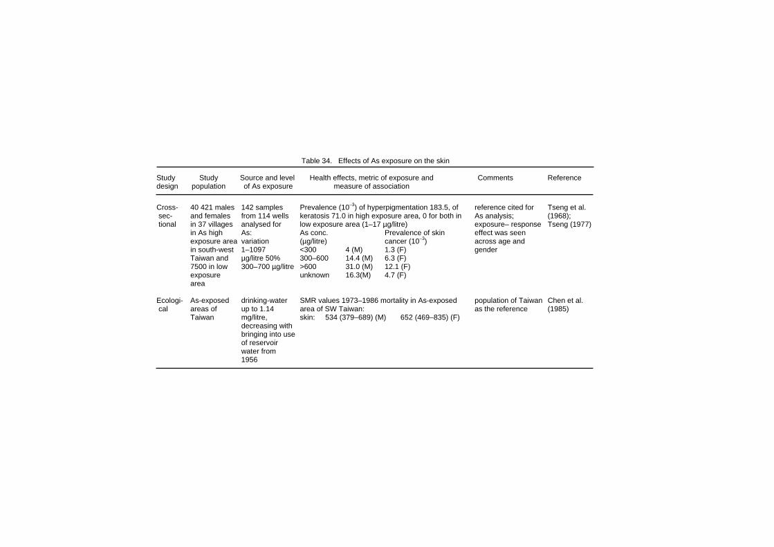
Table 34. Effects of As exposure on the skin Study Study Source and level Health effects, metric of exposure and Comments Reference design population of As exposure measure of association Cross- 40 421 males 142 samples Prevalence (10–3) of hyperpigmentation 183.5, of reference cited for Tseng et al. sec- and females from 114 wells keratosis 71.0 in high exposure area, 0 for both in As analysis; (1968); tional in 37 villages analysed for low exposure area (1–17 µg/litre) exposure– response Tseng (1977) in As high As: As conc. Prevalence of skin effect was seen exposure area variation (µg/litre) cancer (10–3) across age and in south-west 1–1097 <300 4 (M) 1.3 (F) gender Taiwan and µg/litre 50% 300–600 14.4 (M) 6.3 (F) 7500 in low 300–700 µg/litre >600 31.0 (M) 12.1 (F) exposure unknown 16.3(M) 4.7 (F) area Ecologi- As-exposed drinking-water SMR values 1973–1986 mortality in As-exposed population of Taiwan Chen et al. cal areas of up to 1.14 area of SW Taiwan: as the reference (1985) Taiwan mg/litre, skin: 534 (379–689) (M) 652 (469–835) (F) decreasing with bringing into use of reservoir water from 1956

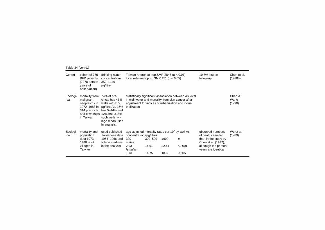
Table 34 (contd.) Cohort cohort of 789 drinking-water Taiwan reference pop.SMR 2846 (p < 0.01) 10.6% lost on Chen et al. BFD patients concentrations local reference pop. SMR 451 (p < 0.05) follow-up (1988b) (7278 person- 350–1140 years of µg/litre observation) Ecologi- mortality from 74% of pre- statistically significant association between As level Chen & cal malignant cincts had <5% in well-water and mortality from skin cancer after Wang neoplasms in wells with ≥ 50 adjustment for indices of urbanization and indus- (1990) 1972–1983 in µg/litre As, 15% trialization 314 precincts has 5–14% and and townships 12% had ≥15% in Taiwan such wells; vil- lage mean used in analysis. Ecologi- mortality and used published age-adjusted mortality rates per 105 by well As observed numbers Wu et al. cal population Taiwanese data concentration (µg/litre) of deaths smaller (1989) data 1973– 1964–1966 and 300 300–599 ≥600 p than in the study by 1986 in 42 village medians males: Chen et al. (1992), villages in in the analysis 2.03 14.01 32.41 <0.001 although the person- Taiwan females: years are identical 1.73 14.75 18.66 <0.05

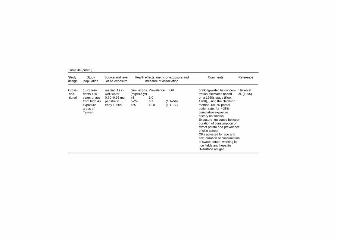
Table 34 (contd.) Study Study Source and level Health effects, metric of exposure and Comments Reference design population of As exposure measure of association Cross- 1571 resi- median As in cum. expos. Prevalence OR drinking-water As concen- Hsueh et sec- dents >30 well-water (mg/litre-yr) tration estimates based al. (1995) tional years of age 0.70–0.93 mg ≤4 1.0 on a 1960s study (Kuo, from high As per litre in 5–24 6.7 (1.1–59) 1968), using the Natelson exposure early 1960s ≥25 13.8 (1.1–77) method. 68.8% partici- areas of pation rate, for ~25% Taiwan cumulative exposure history not known Exposure–response between duration of consumption of sweet potato and prevalence of skin cancer ORs adjusted for age and sex, duration of consumption of sweet potato, working in rice fields and hepatitis B–surface antigen

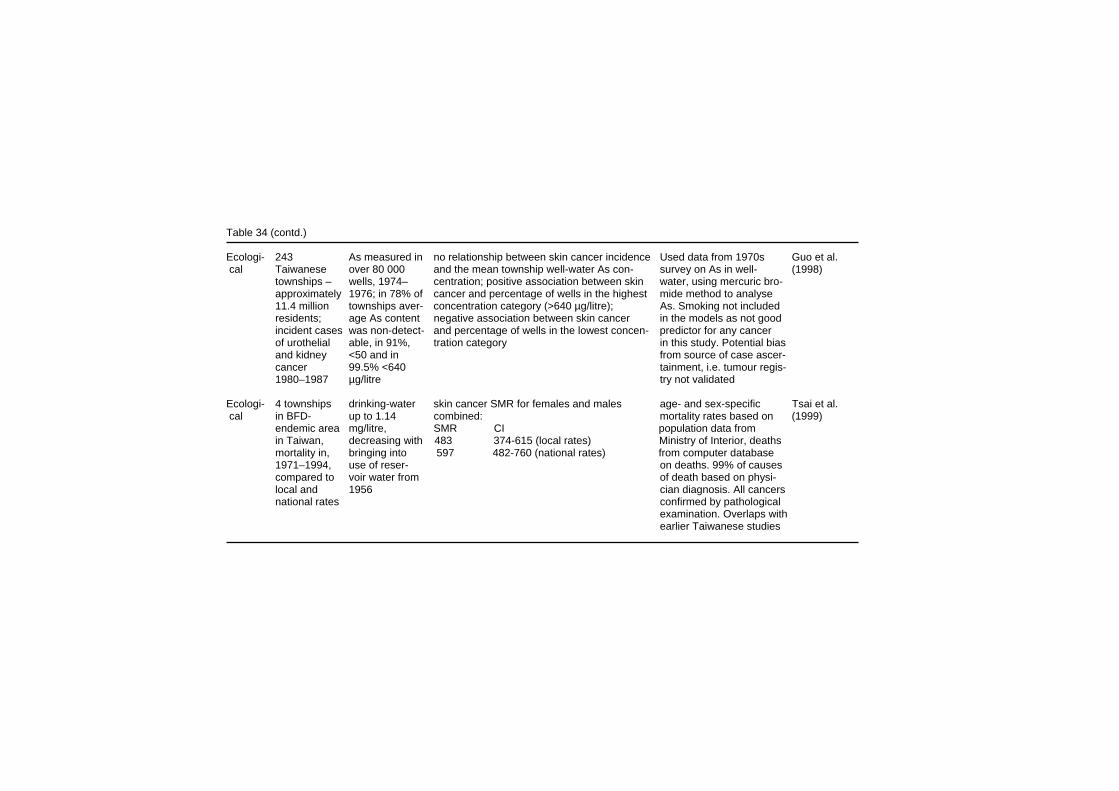
Table 34 (contd.) Ecologi- 243 As measured in no relationship between skin cancer incidence Used data from 1970s Guo et al. cal Taiwanese over 80 000 and the mean township well-water As con- survey on As in well- (1998) townships – wells, 1974– centration; positive association between skin water, using mercuric bro- approximately 1976; in 78% of cancer and percentage of wells in the highest mide method to analyse 11.4 million townships aver- concentration category (>640 µg/litre); As. Smoking not included residents; age As content negative association between skin cancer in the models as not good incident cases was non-detect- and percentage of wells in the lowest concen- predictor for any cancer of urothelial able, in 91%, tration category in this study. Potential bias and kidney <50 and in from source of case ascer- cancer 99.5% <640 tainment, i.e. tumour regis- 1980–1987 µg/litre try not validated Ecologi- 4 townships drinking-water skin cancer SMR for females and males age- and sex-specific Tsai et al. cal in BFD- up to 1.14 combined: mortality rates based on (1999) endemic area mg/litre, SMR CI population data from in Taiwan, decreasing with 483 374-615 (local rates) Ministry of Interior, deaths mortality in, bringing into 597 482-760 (national rates) from computer database 1971–1994, use of reser- on deaths. 99% of causes compared to voir water from of death based on physi- local and 1956 cian diagnosis. All cancers national rates confirmed by pathological examination. Overlaps with earlier Taiwanese studies

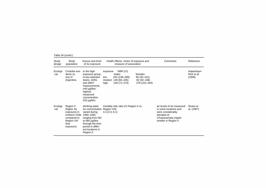
Table 34 (contd.) Study Study Source and level Health effects, metric of exposure and Comments Reference design population of As exposure measure of association Ecologi- Cordoba resi- in the high- exposure SMR (CI) Hopenhayn- cal dents vs. exposure group, males females Rich et al. rest of in two selected low 204 (138–289) 85 (42–151) (1998) Argentina towns, 42/61 medium 149 (83–245) 82 (32–168) and 49/57 high 149 (71–273) 278 (161–444) measurements ≥40 µg/litre; highest measured concentration 533 µg/litre Ecologi- Region II drinking-water mortality rate ratio (CI Region II vs. air levels of As measured Rivara et cal (higher As As concentration Region VIII) in some locations and al. (1997) exposure) in varied during 4.3 (2.3–5.1) were considerably northern Chile 1950–1992, elevated at compared to ranging from ND Chuquicamata copper Region VIII to 860 µg/litre smelter in Region II. (low through the time exposure) period in differ- ent locations in Region II.

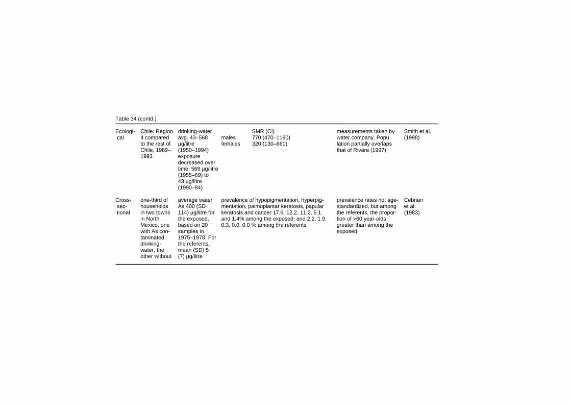
Table 34 (contd.) Ecologi- Chile: Region drinking-water SMR (CI) measurements taken by Smith et al. cal II compared avg. 43–568 males 770 (470–1190) water company. Popu (1998) to the rest of µg/litre females 320 (130–660) lation partially overlaps Chile, 1989– (1950–1994) that of Rivara (1997) 1993 exposure decreased over time: 569 µg/litre (1955–69) to 43 µg/litre (1990–94) Cross- one-third of average water prevalence of hypopigmentation, hyperpig- prevalence rates not age- Cebrian sec- households As 400 (SD mentation, palmoplantar keratosis, papular standardized, but among et al. tional in two towns 114) µg/litre for keratosis and cancer 17.6, 12.2, 11.2, 5.1 the referents, the propor- (1983) in North the exposed, and 1.4% among the exposed, and 2.2, 1.9, tion of >60 year-olds Mexico, one based on 20 0.3, 0.0, 0.0 % among the referents greater than among the with As con- samples in exposed taminated 1975–1978. For drinking- the referents, water, the mean (SD) 5 other without (7) µg/litre

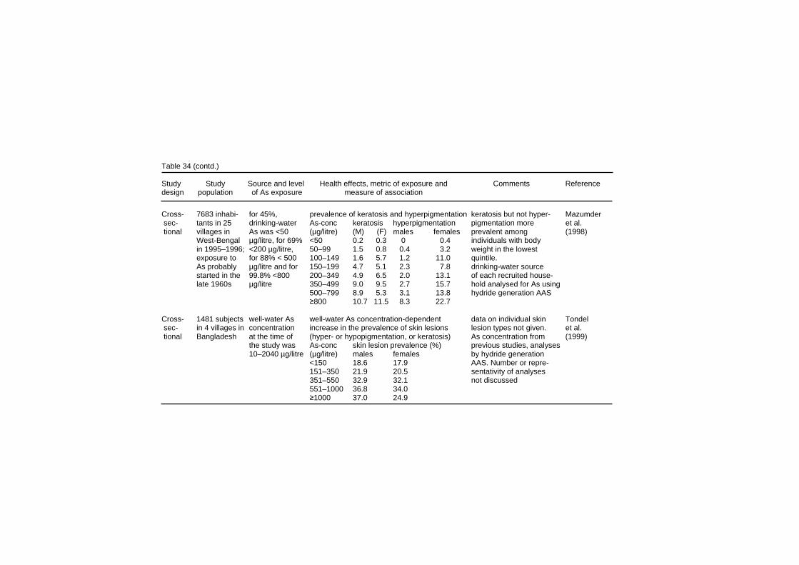
Table 34 (contd.) Study Study Source and level Health effects, metric of exposure and Comments Reference design population of As exposure measure of association Cross- 7683 inhabi- for 45%, prevalence of keratosis and hyperpigmentation keratosis but not hyper- Mazumder sec- tants in 25 drinking-water As-conc keratosis hyperpigmentation pigmentation more et al. tional villages in As was <50 (µg/litre) (M) (F) males females prevalent among (1998) West-Bengal µg/litre, for 69% <50 0.2 0.3 0 0.4 individuals with body in 1995–1996; <200 µg/litre, 50–99 1.5 0.8 0.4 3.2 weight in the lowest exposure to for 88% < 500 100–149 1.6 5.7 1.2 11.0 quintile. As probably µg/litre and for 150–199 4.7 5.1 2.3 7.8 drinking-water source started in the 99.8% <800 200–349 4.9 6.5 2.0 13.1 of each recruited house- late 1960s µg/litre 350–499 9.0 9.5 2.7 15.7 hold analysed for As using 500–799 8.9 5.3 3.1 13.8 hydride generation AAS ≥800 10.7 11.5 8.3 22.7 Cross- 1481 subjects well-water As well-water As concentration-dependent data on individual skin Tondel sec- in 4 villages in concentration increase in the prevalence of skin lesions lesion types not given. et al. tional Bangladesh at the time of (hyper- or hypopigmentation, or keratosis) As concentration from (1999) the study was As-conc skin lesion prevalence (%) previous studies, analyses 10–2040 µg/litre (µg/litre) males females by hydride generation <150 18.6 17.9 AAS. Number or repre- 151–350 21.9 20.5 sentativity of analyses 351–550 32.9 32.1 not discussed 551–1000 36.8 34.0 ≥1000 37.0 24.9

Effects on Humans The SMR from skin cancer in the BFD-endemic area was 534 (CI 379–689) in men and 652 (CI 469–835) in women in the first ecological study in south-western Taiwan (Chen et al., 1985). The skin cancer SMR among BFD patients in this population during a 15-year follow-up was 2846 in comparison to the Taiwanese population, and 451 in comparison to the population in the endemic area without BFD (Chen et al., 1988b). Multivariate analysis, adjusting for indices of urbanization and industrialization, revealed a statistically significant association between arsenic level in well-water and mortality from skin cancer (Chen & Wang, 1990). In the second ecological study in this area (Wu et al., 1989), age-adjusted mortality rates from skin cancer for men were 2.03 × 10–5, 14.01 × 10–5 and 32.41 × 10–5 in villages with a median well arsenic concentration of < 300, 300–600 and > 600 µg/litre, respectively, and there was a similar exposure–response relationship for women (for study descriptions, see section 8.4). In 1988–1989 a survey was carried out to investigate the relationship of arsenic exposure to skin cancer in three villages in the BFD-endemic area of Taiwan (Hsueh et al., 1995), in which 1571 habitants of the three villages, who lived in one of the villages no less than 5 days a week (out of a total population of 2258), were interviewed for their drinking-water consumption and other personal history. Of these, 1081 (68.8%) participated in a physical examin-ation, and were included in the analysis. Altogether 66 cases of skin cancer were diagnosed, and the age- and sex-adjusted prevalence OR of skin cancer was related to all parameters of arsenic exposure, i.e. village well-water mean arsenic concentration (from analyses in the early 1960s), duration of living in the BFD-endemic area, duration of drinking artesian well-water and cumulative arsenic exposure. For well-water arsenic concentration, the OR was 3.5 (CI 0.7–17.0) and 5.0 (1.1–23.8) for concentrations 0–700 and > 700 µg/litre, respectively. Skin cancer incidence in 1980–1987 was studied in the 243 townships in Taiwan, where the arsenic concentrations in some 83 000 wells had been investigated in the 1974–1976 survey (Guo et al., 1998). A total of 1547 skin cancer cases were identified, and demographic data on the study population was obtained from the Department of Internal Affairs. Sex-specific age-adjusted standardized incidence rates were calculated for each township. No

315

EHC 224: Arsenic and Arsenic Compounds relationship was observed between skin cancer incidence and the mean township arsenic concentration in the well-water. However, when a multiple-variable analysis was applied, using the percentage of wells within a township with a specified range or arsenic concentrations as the parameter describing exposure, a positive association was observed at the highest arsenic exposure category (> 640 µg/litre) for both men and women. In the most recent ecological study in the area (Tsai et al., 1999), an elevated mortality from skin cancer (SMR 483, CI 374–615, and 597 in comparison to the local, and national figures for men and women combined), was also observed (for study description, see section 8.4.2). In the ecological study in Argentina (Hopenhayn-Rich et al., 1998; for study description, see section 8.7.2), the mortality from skin cancer showed a negative association with arsenic exposure in men and a positive association in women. In the mortality study in Chile in 1989–1993 (Smith et al., 1998), the SMR for skin cancer in Region II with elevated arsenic drinking-water concentration was 770 (CI 470–1190) in men, and 320 (130–660) in women, compared to the figures for the whole of Chile. The excess skin cancer mortality in Region II was similar in the comparison with Region VIII (Rivara et al., 1997), in which cases from 1950–1992 were studied (RR 4.3, CI 2.3–5.1 for both sexes combined) (For study descriptions, see section 8.7.2.) Cebrian et al. (1983) conducted a cross-sectional study of skin lesions in two towns in Mexico. The average arsenic concentration of water samples in the exposed town was 0.411 mg/litre; the average concentration in the control town was 0.005 mg/litre. The subjects examined were selected for examination by systematic sampling of the populations in the two towns: 296 individuals from the exposed population of 998 and 318 individuals from the control population of 1488 were physically examined. In the exposed town, there were 52 cases (17.6%) of hypopigmentation, 36 cases of hyperpigmentation (12.2%), 33 cases (11.2%) of palmoplantar keratosis, 15 cases (5.1%) of papular keratosis, and 4 cases (1.4%) of ulcerative zones (skin cancer). In the control town, there were 7 cases (2.2%) of hypopigmentation, 6 cases (1.9%) of hyperpigmen-

316

Effects on Humans tation, 1 case (0.3%) of palmoplantar keratosis, no cases of papular keratosis, and no cases of ulcerative zones (skin cancer). The prevalence of all the skin lesions was significantly elevated in the exposed town (p < 0.001, with the exception of ulcerative zones which had p = 0.04) and was generally found to increase with age. Non-specific symptoms (e.g. nausea, epigastric pain, colic abdominal pain, diarrhoea, headache, and oedema) were found to be more prevalent in the exposed town than the control town and more common among those with skin lesions. The relationship between skin keratosis and hyperpigmentation and consumption of arsenic-contaminated drinking-water was investigated in a cross-sectional study of a population in West Bengal (India) (Mazumder et al., 1998). There were 7683 participants from areas of both high and low arsenic-exposure. Each participant was questioned about drinking-water sources, water intake, diet, medical symptoms, height, weight, and other variables. Participants were medically examined, with a careful inspection for arsenic skin lesions. Water samples were collected from each tube-well used by the households of the participants in the study. The age-adjusted prevalence of keratosis rose from zero in the lowest exposure level (< 50 µg As/litre) to 8.3 per 100 for females drinking-water containing > 800 µg As/litre. For males, the age-adjusted prevalence of keratosis increased from 0.2 per 100 in the lowest exposure category to 10.7 per 100 for males in the highest exposure level (> 800 µg As/litre). For females, the age-adjusted prevalence of hyperpigmentation rose from 0.3 per 100 in the lowest exposure category to 11.5 per 100 in the highest exposure category; for males the age-adjusted prevalence rose from 0.4 per 100 in the lowest exposure category to 22.7 per 100 in the highest exposure category. Comparison by dose per body weight found that men had roughly 2–3 times the prevalence of both keratosis and hyperpigmentation compared to women apparently ingesting the same dose of arsenic from drinking-water. Subjects below 80% of their body weight for their age and sex had a 1.6-fold (CI 1.0–2.4) increase in the prevalence of keratoses, suggesting that malnutrition may play a role in increasing susceptibility. No such difference was observed for hyperpigmentation. Twelve subjects with keratosis drank water containing < 100 µg As/litre; 29 with hyperpigmentation drank water containing < 100 µg As/litre.

317

EHC 224: Arsenic and Arsenic Compounds Tondel et al. (1999) examined 1481 subjects ≥30 years of age in four villages in Bangladesh. All were determined to have had a history of arsenic exposure through arsenic-contaminated drinking-water. Arsenic concentrations in the drinking-water ranged from 10 to 2040 µg As/litre. Of the 1481 people examined, 430 were found to have skin lesions (pigmentation changes or keratosis). The age-adjusted prevalence rate of skin lesions was found to increase from 18.6 per 100 in the lowest exposure category (≤150 µg As/litre) to 37.0 per 100 in the highest exposure category (> 1000 µg As/litre) for males and from 17.9 per 100 in the lowest exposure category to 24.9 per 100 in the highest exposure category for females. The trend was statistically significant for both males and females. When the exposure was considered by dose (µg/litre ⋅ kg), there was also an increase in the age-adjusted prevalence rate of skin lesions for both males and females across dose groups, the trend being statistically significant. A clinical study of 11 families from a village in northern Chile, supplied by water containing up to 800 µg As/litre, found skin changes in 6 of 44 subjects despite good nutritional status (Smith et al., 2000). Arsenic exposure in this village is reported to have been present for thousands of years, suggesting that there has been no adaptation to arsenic exposure by the population. Arsenite can induce an irritative contact dermatitis after occupational exposure (Goncalo et al., 1980), but dermal sensiti-zation to inorganic arsenic appears to be a rare occurrence. Barbaud et al. (1995) reported on the contact hypersensitivity of arsenic in a crystal factory employee. A patch test was done with various compounds that he came in contact with at work, and arsenate was the only chemical that tested positive.

8.8 Reproductive toxicity (Table 35) A series of reproductive outcomes have been examined among female employees and women living close to the Rönnskär copper smelter in Sweden. Nordstrom et al. (1978a) compared birth weights of all offspring of women employed at the Rönnskär smelter during a 2-year period (1975–1976), categorized in three main groups according to their work location: factory, laboratory and administration. Information was also collected for infants of women

318

Effects on Humans who lived in four areas close to the smelter but at increasing distances. Births from the University Hospital in Umeå, a city distant from the smelter, were used as external controls. The average birth weight of infants of Rönnskär employees and of women living closer to the smelter were significantly lower than those from the two more distant areas and from Umeå. Among employees, those working in the laboratory had larger babies than those in the factory or in administration. In general, the effect was mainly observed in higher pregnancy orders (second born or later). Contrary to what is generally observed, there was a decrease in the average birth weight of offspring of higher parity among employees. Nordstrom et al. (1978b) reviewed data from hospital files on over 4427 pregnancies of women born in or after 1930 who lived in four areas of increasing distances from the smelter. A control group of 4544 pregnancies was used from a hospital in Umeå, a non-exposed town. There was a clear dose–response relationship between the occurrence of spontaneous abortions and residential proximity to the smelter. In particular, women in the closest town (< 10 km from the smelter) had the highest rates (11% vs. 7.6%, p < 0.005). In the most exposed area, 4 of 20 women with abortions had had 2 abortions and no normal pregnancies. No women with such reproductive history were found in the other three areas. In a further study (Nordstrom et al., 1979a), the previous analysis (Nordstrom et al., 1978a,b) was expanded to cover 662 births among women employed in or living near the smelter and in the unexposed town of Umeå in 1930–1959. Personal questionnaires were used to assess exposure and confounding factors. The average birth weight of babies born to employees was significantly lower than those born in Umeå (p < 0.05); in addition, birth weight was lower if the mother worked in the highest exposure categories (e.g. smelting and cleaning operations) rather than in lower exposure jobs. Most differences were found for the birth weight of third or later-born infants, which the authors proposed to be caused by the cumulative exposure with age. The differences were not found to be confounded by the gestational ages. Spontaneous abortions were highest when the mother was employed during pregnancy (14%) or before pregnancy and living near the smelter. Within employment categories, significantly higher rates of abortion were observed in high exposure jobs (28% vs. 14%, NS). The abortion rate was even

319

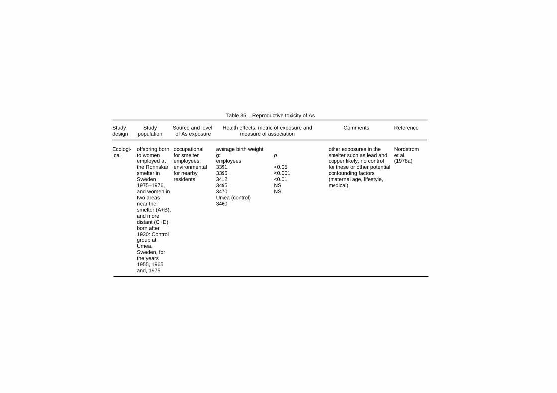
Table 35. Reproductive toxicity of As Study Study Source and level Health effects, metric of exposure and Comments Reference design population of As exposure measure of association Ecologi- offspring born occupational average birth weight other exposures in the Nordstrom cal to women for smelter g: p smelter such as lead and et al. employed at employees, employees copper likely; no control (1978a) the Ronnskar environmental 3391 <0.05 for these or other potential smelter in for nearby 3395 <0.001 confounding factors Sweden residents 3412 <0.01 (maternal age, lifestyle, 1975–1976, 3495 NS medical) and women in 3470 NS two areas Umea (control) near the 3460 smelter (A+B), and more distant (C+D) born after 1930; Control group at Umea, Sweden, for the years 1955, 1965 and, 1975

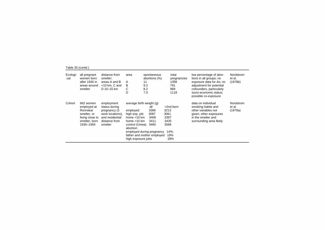
Table 35 (contd.) Ecologi- all pregnant distance from area spontaneous total low percentage of abor- Nordstrom cal women born smelter: abortions (%) pregnancies tions in all groups; no et al. after 1930 in areas A and B A 11 1358 exposure data for As; no (1978b) areas around <10 km, C and B 9.2 791 adjustment for potential smelter D 10–15 km C 8.2 969 cofounders, particularly D 7.0 1118 socio-economic status; possible co-exposure Cohort 662 women employment average birth weight (g) data on individual Nordstrom employed at status during all >2nd born smoking habits and et al. Ronnskar pregnancy (3 employed 3366 3213 other variables not (1979a) smelter, or work locations), high exp. job 3087 3061 given; other exposures living close to and residential home <10 km 3406 3397 in the smelter and smelter, born distance from home >10 km 3411 3435 surrounding area likely 1930–1959 smelter control (Umea) 3460 3568 abortion: employed during pregnancy 14%; father and mother employed 19% high exposure jobs 28%

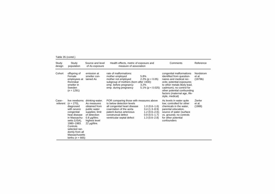
Table 35 (contd.) Study Study Source and level Health effects, metric of exposure and Comments Reference design population of As exposure measure of association Cohort offspring of emission at rate of malformations: congenital malformations Nordstrom Female smelter con- mother employed 5.8% identified from question- et al. employees at tained As mother not employed 2.2% (p < 0.05) naires and medical rec- (1979b) Ronnskar subgroup of mothers (born after 1930): ords; potential exposures smelter in emp. before pregnancy 3.2% to other metals likely lead, Sweden emp. during pregnancy 5.1% (p < 0.025) cadmium); no control for (n = 1291) other potential confounding factors (maternal age, life- style, medical) Case– live newborns drinking-water. POR comparing those with measures above As levels in water quite Zierler referent (n = 270), As measures to below detection levels low; controlled for other et al. diagnosed obtained from all congenital heart disease 1.0 (0.6–1.6) chemicals in the water, (1988) with severe public water coarctation of the aorta 3.4 (1.3–8.9) parental education, congenital supplies; limit patent ductus arteriosus 1.2 (0.6–2.6); source of water (surface heat disease of detection conotruncal defect 0.9 (0.5–1.7) vs. ground); no controls in Massachu- 0.8 µg/litre; ventricular septal defect 1.3 (0.6–2.8) for other potential setts (USA), highest level confounders 1980–1983. 22 µg/litre. Controls selected ran- domly from all Massachusetts births (n = 665)

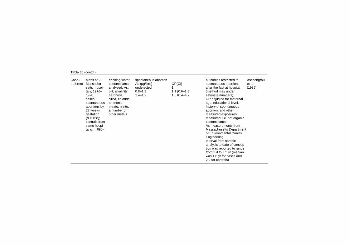
Table 35 (contd.) Case– births at 2 drinking-water spontaneous abortion outcomes restricted to Aschengrau referent Massachu- contaminants As (µg/litre) OR(CI) spontaneous abortions et al. setts hospi- analysed: As, undetected: 1 after the fact at hospital (1989) tals, 1976– pH, alkalinity, 0.8–1.3 1.1 (0.6–1.8) (method may under 1978 hardness, 1.4–1.9 1.5 (0.4–4.7) estimate numbers); cases: silica, chloride, OR adjusted for maternal spontaneous ammonia, age, educational level, abortions by nitrate, nitrite, history of spontaneous 27 weeks a number of abortion, and other gestation other metals measured exposures (n = 158); measured, i.e. not organic controls from contaminants same hospi- As measurements from tal (n = 690) Massachusetts Department of Environmental Quality Engineering Interval from sample analysis to date of concep- tion was reported to range from 5 d to 3.5 yr (median was 1.6 yr for cases and 2.2 for controls)

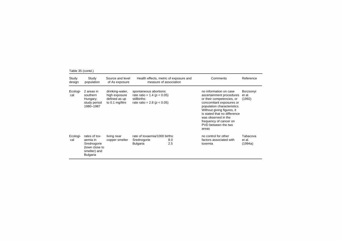
Table 35 (contd.) Study Study Source and level Health effects, metric of exposure and Comments Reference design population of As exposure measure of association Ecologi- 2 areas in drinking-water, spontaneous abortions: no information on case Borzsonyi cal southern high exposure rate ratio = 1.4 (p < 0.05) ascertainment procedures et al. Hungary; defined as up stillbirths: or their competencies, or (1992) study period to 0.1 mg/litre rate ratio = 2.8 (p < 0.05) concomitant exposures or 1980–1987 population characteristics. Without giving figures, it is stated that no difference was observed in the frequency of cancer on PVD between the two areas Ecologi- rates of tox- living near rate of toxaemia/1000 births: no control for other Tabacova cal aemia in copper smelter Srednogorie 8.0 factors associated with et al. Srednogorie Bulgaria 2.5 toxemia (1994a) (town close to smelter) and Bulgaria

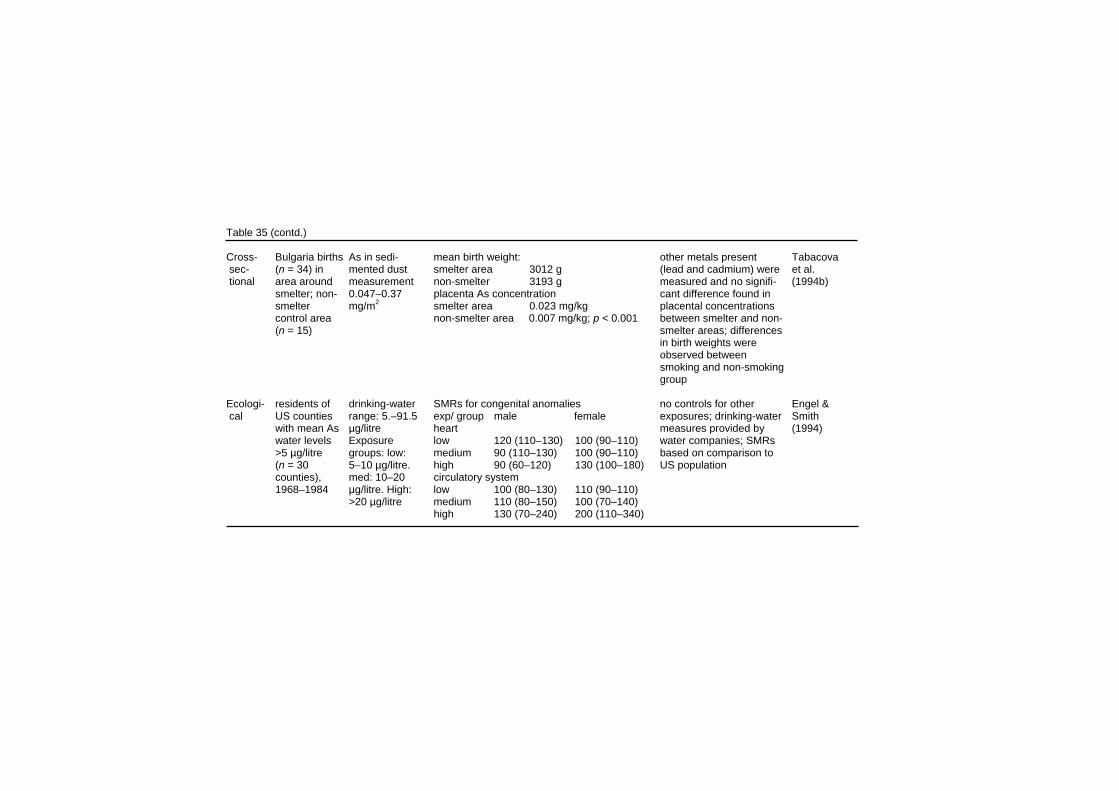
Table 35 (contd.) Cross- Bulgaria births As in sedi- mean birth weight: other metals present Tabacova sec- (n = 34) in mented dust smelter area 3012 g (lead and cadmium) were et al. tional area around measurement non-smelter 3193 g measured and no signifi- (1994b) smelter; non- 0.047–0.37 placenta As concentration cant difference found in smelter mg/m2 smelter area 0.023 mg/kg placental concentrations control area non-smelter area 0.007 mg/kg; p < 0.001 between smelter and non- (n = 15) smelter areas; differences in birth weights were observed between smoking and non-smoking group Ecologi- residents of drinking-water SMRs for congenital anomalies no controls for other Engel & cal US counties range: 5.–91.5 exp/ group male female exposures; drinking-water Smith with mean As µg/litre heart measures provided by (1994) water levels Exposure low 120 (110–130) 100 (90–110) water companies; SMRs >5 µg/litre groups: low: medium 90 (110–130) 100 (90–110) based on comparison to (n = 30 5–10 µg/litre. high 90 (60–120) 130 (100–180) US population counties), med: 10–20 circulatory system 1968–1984 µg/litre. High: low 100 (80–130) 110 (90–110) >20 µg/litre medium 110 (80–150) 100 (70–140) high 130 (70–240) 200 (110–340)

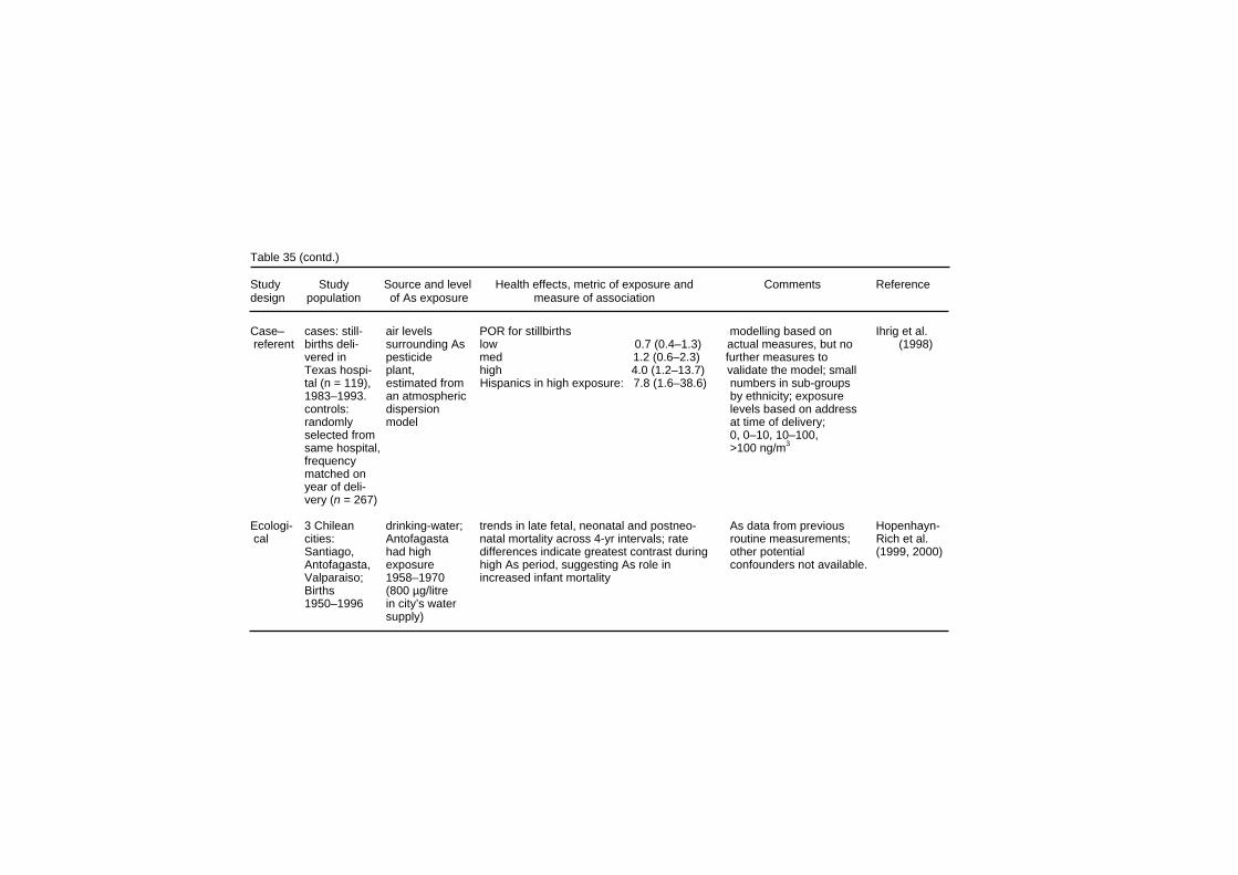
Table 35 (contd.) Study Study Source and level Health effects, metric of exposure and Comments Reference design population of As exposure measure of association Case– cases: still- air levels POR for stillbirths modelling based on Ihrig et al. referent births deli- surrounding As low 0.7 (0.4–1.3) actual measures, but no (1998) vered in pesticide med 1.2 (0.6–2.3) further measures to Texas hospi- plant, high 4.0 (1.2–13.7) validate the model; small tal (n = 119), estimated from Hispanics in high exposure: 7.8 (1.6–38.6) numbers in sub-groups 1983–1993. an atmospheric by ethnicity; exposure controls: dispersion levels based on address randomly model at time of delivery; selected from 0, 0–10, 10–100, same hospital, >100 ng/m3 frequency matched on year of deli- very (n = 267) Ecologi- 3 Chilean drinking-water; trends in late fetal, neonatal and postneo- As data from previous Hopenhayn- cal cities: Antofagasta natal mortality across 4-yr intervals; rate routine measurements; Rich et al. Santiago, had high differences indicate greatest contrast during other potential (1999, 2000) Antofagasta, exposure high As period, suggesting As role in confounders not available. Valparaiso; 1958–1970 increased infant mortality Births (800 µg/litre 1950–1996 in city’s water supply)

Effects on Humans higher if the father also worked at the smelter, not just the mother (19% vs. 14%; statistical significance not provided). Individual smoking data was not given, although no differences were found between the smoking rates of the different groups. Nordstrom et al. (1979b), in an investigation of the occurrence of congenital malformations, found rates of 5.8% among infants born to female employees who worked at the smelter during pregnancy, compared to 2.2% among female employees who did not work (p < 0.005) and 3% among residents in the larger region. Multiple malformations were four times more common among employees working during pregnancy than among residents in the larger region. Most of these studies by Nordstrom and co-workers had an ecological design with little or no information on other factors. Although arsenic exposures in and around the Rönnskär smelter were high, confounding from lead or copper could not be excluded. In addition, no adjustments were made for the effects of other potential confounding risk factors, such as maternal age, which is known to have a strong relationship to spontaneous abortion and congenital anomalies. Zierler et al. (1988) compared 270 cases of infants born with congenital heart disease and 665 controls from Massachusetts (USA). The POR, adjusted for all measured contaminants, source of water, and maternal education, for any congenital heart disease in relation to any arsenic exposure above the detection limit of 0.8 µg/litre, was not elevated. However, for a specific malformation, coarctation of the aorta, there was a significant POR of 3.4 (1.3–8.9). The exposure was quite low, the 90th percentile level being 1 µg/litre. On the basis of information from a previous case–control study of spontaneous abortions in Boston, Aschengrau et al. (1989) examined 286 women who experienced spontaneous abortions and 1391 controls in relation to the content of their water supplies. An adjusted odds ratio of 1.5 was found for the group with the highest arsenic concentrations. However, this exposure group had low levels of arsenic in water (1.4–1.9 µg/litre), close to or lower than laboratory analytical detection limits, and the possibility of chance or unaccounted confounders could not be discounted.

327

EHC 224: Arsenic and Arsenic Compounds A study in an area of south-east Hungary (Borzsonyi et al., 1992) with exposure to arsenic from drinking-water examined the rates of spontaneous abortions and stillbirths for the period 1980-1987. Two populations were compared: one with levels of arsenic in drinking-water > 100 µg/litre (n = 25 648 people) and one control area with low arsenic levels (n = 20 836) (no information on analytical method, or timing or frequency of sampling was available). Both outcomes were significantly higher in the exposed groups, with a 1.4-fold increase in spontaneous abortions (p = 0.007) and a 2.8-fold increase in stillbirths (p = 0.028). Although both populations were reported to be similar in several characteristics, such as smoking, lifestyle, occupation and socio-economic status, no information was provided, and other important factors such as smoking and maternal age were not accounted for. Furthermore, no mention was made of other potential environmental exposures; in populations of roughly similar size, the number of live births during the study period, 1980–1987 was 5218 in the high- and 2112 in the low-exposure area; it was stated that no significant differences were observed in the cancer frequency; the frequency of spontaneous abortions was unusually low, 7 and 5%, respectively. A retrospective analysis (Tabacova et al., 1994a) compared the 5-year incidence rate of toxaemia of pregnancy in Srednogorie, a small town in Bulgaria located 2 km from a copper smelter, to the Bulgarian national rates. Data was derived from local and central morbidity registers. The incidence of toxaemia was more than three times greater around the smelter (8.0 vs. 2.5 per 1000 births). However, this report did not present any information regarding other factors or exposures that could be associated with the rate differences. The study also followed 71 pregnancies in Strednogorie, including measurement of urinary arsenic. The levels reported do not appear to reflect high environmental arsenic exposures. Another study in Bulgaria (Tabacova et al., 1994b) included 34 maternal–infant pairs from the smelter area and 15 from a non-smelter area free from industrial exposures. Information regarding lifestyle characteristics, occupation, residence and medical history was ascertained by personal interviews. Samples of maternal and cord blood and placenta were obtained for analysis of arsenic, cadmium and lead concentrations. Infants born in the proximity of the smelter had lower birth weight (3012 vs. 3193 g). Although the

328

Effects on Humans study was small, these differences were also observed when divided into smoking and parity sub-groups. Placental concentrations of arsenic were three times higher (p < 0.001) in the smelter area, but cadmium levels were also elevated although the difference was not statistically significant. There was no difference in average lead levels in the two exposure areas. A study conducted in the USA (Engel & Smith, 1994) investigated mortality from vascular diseases in the 30 counties with the highest average levels of arsenic in drinking-water for the period 1968–1984. The levels ranged from 5.4 µg/litre in Pierce County, Washington to 92 µg/litre in Churchill County, Nevada. When counties were grouped in three arsenic exposure categories, defined as 5–10, 10–20 and > 20 µg/litre, there appeared to be an increase in mortality from congenital anomalies of the heart only for females in the highest exposure group (SMR = 130, 90% CI (100–180), and for both sexes for congenital anomalies of the circulatory system (female SMR = 200, CI (110–340); male SMR = 130, CI (70–240). Slight increases in congenital anomalies of the heart and other anomalies of the circulatory system were found for two counties in the highest exposure group (29 and 46 µg As/litre in water, respectively), but none were found for Churchill County, which has the highest arsenic levels (92.5 µg/litre). A hospital case–control study in the USA investigated the occurrence of stillbirths in relation to residential proximity to an arsenical pesticide production plant in Texas (Ihrig et al., 1998). Exposure was categorized in three groups according to arsenic air levels. An increasing, but not significant, trend in the risk of stillbirths was observed. The number of stillbirths was significantly elevated for the high-exposure group. When stratified by ethnicity, however, the findings remained significant for Hispanics only. Other exposures from the chemical plant were possible and were not measured in the study. An ecological study examined infant mortality rates in three Chilean cities over a 46-year period (1950–1996) (Hopenhayn-Rich et al., 1999, 2000) (Fig. 4). Antofagasta, in northern Chile, experienced very high arsenic levels in drinking-water for a period of 12 years. In 1958 a new water source which contained arsenic concentrations around 800 µg/litre was introduced as the main

329

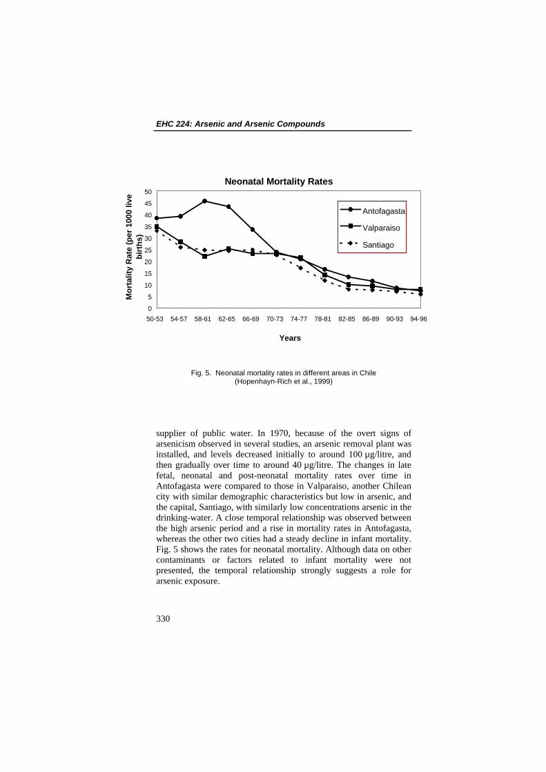
EHC 224: Arsenic and Arsenic Compounds

Neonatal Mortality Rates

0

5

10

15

20

25

30

35

40

45

50

50-53 54-57 58-61 62-65 66-69 70-73 74-77 78-81 82-85 86-89 90-93 94-96

Years

Mor

talit

y R

ate

(per

100

0 liv

e bi

rths

)

Antofagasta

Valparaiso

Santiago

Fig. 5. Neonatal mortality rates in different areas in Chile (Hopenhayn-Rich et al., 1999)

supplier of public water. In 1970, because of the overt signs of arsenicism observed in several studies, an arsenic removal plant was installed, and levels decreased initially to around 100 µg/litre, and then gradually over time to around 40 µg/litre. The changes in late fetal, neonatal and post-neonatal mortality rates over time in Antofagasta were compared to those in Valparaiso, another Chilean city with similar demographic characteristics but low in arsenic, and the capital, Santiago, with similarly low concentrations arsenic in the drinking-water. A close temporal relationship was observed between the high arsenic period and a rise in mortality rates in Antofagasta, whereas the other two cities had a steady decline in infant mortality. Fig. 5 shows the rates for neonatal mortality. Although data on other contaminants or factors related to infant mortality were not presented, the temporal relationship strongly suggests a role for arsenic exposure.

330

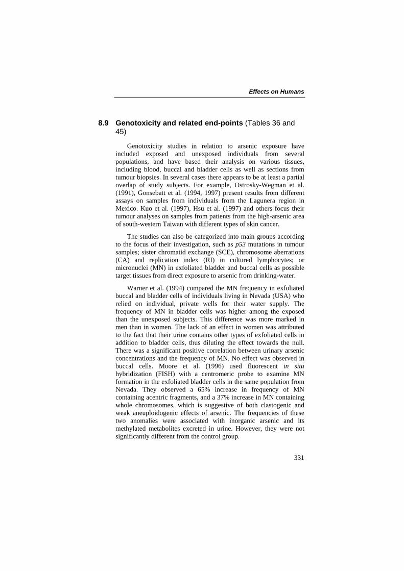
Effects on Humans

8.9 Genotoxicity and related end-points (Tables 36 and 45)

Genotoxicity studies in relation to arsenic exposure have included exposed and unexposed individuals from several populations, and have based their analysis on various tissues, including blood, buccal and bladder cells as well as sections from tumour biopsies. In several cases there appears to be at least a partial overlap of study subjects. For example, Ostrosky-Wegman et al. (1991), Gonsebatt et al. (1994, 1997) present results from different assays on samples from individuals from the Lagunera region in Mexico. Kuo et al. (1997), Hsu et al. (1997) and others focus their tumour analyses on samples from patients from the high-arsenic area of south-western Taiwan with different types of skin cancer. The studies can also be categorized into main groups according to the focus of their investigation, such as p53 mutations in tumour samples; sister chromatid exchange (SCE), chromosome aberrations (CA) and replication index (RI) in cultured lymphocytes; or micronuclei (MN) in exfoliated bladder and buccal cells as possible target tissues from direct exposure to arsenic from drinking-water. Warner et al. (1994) compared the MN frequency in exfoliated buccal and bladder cells of individuals living in Nevada (USA) who relied on individual, private wells for their water supply. The frequency of MN in bladder cells was higher among the exposed than the unexposed subjects. This difference was more marked in men than in women. The lack of an effect in women was attributed to the fact that their urine contains other types of exfoliated cells in addition to bladder cells, thus diluting the effect towards the null. There was a significant positive correlation between urinary arsenic concentrations and the frequency of MN. No effect was observed in buccal cells. Moore et al. (1996) used fluorescent in situ hybridization (FISH) with a centromeric probe to examine MN formation in the exfoliated bladder cells in the same population from Nevada. They observed a 65% increase in frequency of MN containing acentric fragments, and a 37% increase in MN containing whole chromosomes, which is suggestive of both clastogenic and weak aneuploidogenic effects of arsenic. The frequencies of these two anomalies were associated with inorganic arsenic and its methylated metabolites excreted in urine. However, they were not significantly different from the control group.

331

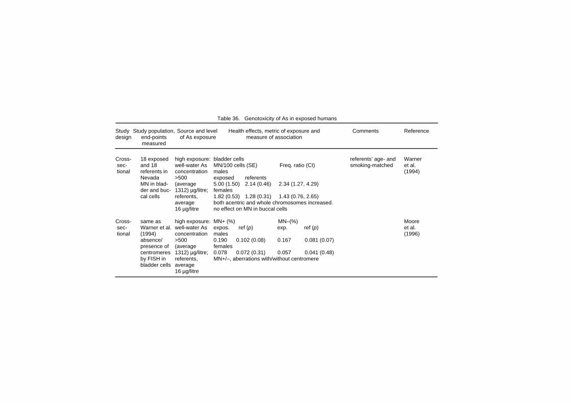
Table 36. Genotoxicity of As in exposed humans Study Study population, Source and level Health effects, metric of exposure and Comments Reference design end-points of As exposure measure of association measured Cross- 18 exposed high exposure: bladder cells referents’ age- and Warner sec- and 18 well-water As MN/100 cells (SE) Freq. ratio (CI) smoking-matched et al. tional referents in concentration males (1994) Nevada >500 exposed referents MN in blad- (average 5.00 (1.50) 2.14 (0.46) 2.34 (1.27, 4.29) der and buc- 1312) µg/litre; females cal cells referents, 1.82 (0.53) 1.28 (0.31) 1.43 (0.76, 2.65) average both acentric and whole chromosomes increased. 16 µg/litre no effect on MN in buccal cells Cross- same as high exposure: MN+ (%) MN–(%) Moore sec- Warner et al. well-water As expos. ref (p) exp. ref (p) et al. tional (1994) concentration males (1996) absence/ >500 0.190 0.102 (0.08) 0.167 0.081 (0.07) presence of (average females centromeres 1312) µg/litre; 0.078 0.072 (0.31) 0.057 0.041 (0.48) by FISH in referents, MN+/–, aberrations with/without centromere bladder cells average 16 µg/litre

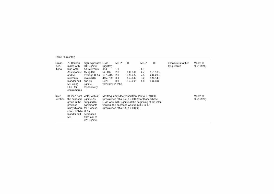
Table 36 (contd.) Cross- 70 Chilean high exposure: U-As MN+* CI MN–* CI exposure stratified Moore et sec- males with 600 µg/litre (µg/litre) by quintiles al. (1997b) tional high water As, referents <54 1.0 1.0 As exposure 15 µg/litre. 54–137 2.3 1.0–5.0 4.7 1.7–13.2 and 50 average U-As 137–415 2.0 0.9–4.5 7.5 2.8–20.3 referents levels 616 415–729 3.1 1.4–6.6 5.2 1.9–14.6 bladder cell and 66 >729 0.9 0.4–2.2 1.0 0.3–3.3 MN using µg/litre, *prevalence ratio FISH for respectively centromeres Inter- 34 men from water with 45 MN frequency decreased from 2.6 to 1.8/1000 Moore et vention the exposed µg/litre As (prevalence ratio 0.7, p < 0.05); for those whose al. (1997c) group in the supplied to U-As was <700 µg/litre at the beginning of the inter- previous participants vention, the decrease was from 3.5 to 1.5 study (Moore for 8 weeks. (prevalence ratio 0.4, p = 0.002). et al., 1997b) U-As bladder cell decreased MN from 742 to 225 µg/litre

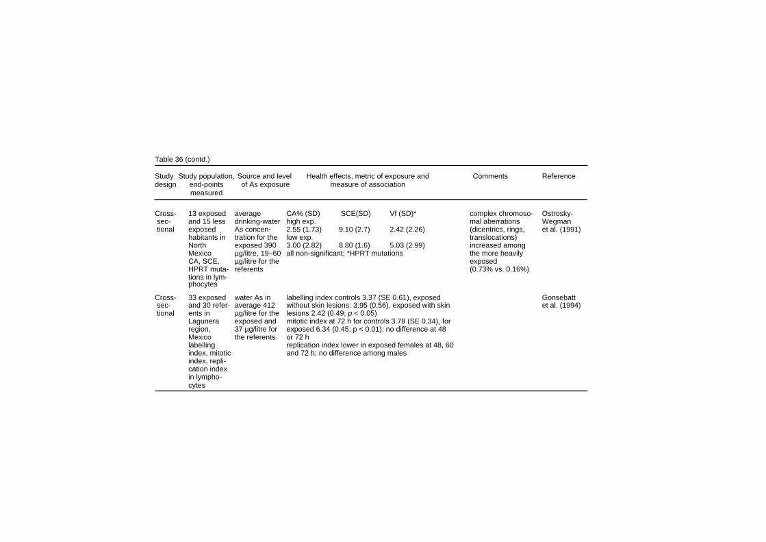
Table 36 (contd.) Study Study population, Source and level Health effects, metric of exposure and Comments Reference design end-points of As exposure measure of association measured Cross- 13 exposed average CA% (SD) SCE(SD) Vf (SD)* complex chromoso- Ostrosky- sec- and 15 less drinking-water high exp. mal aberrations Wegman tional exposed As concen- 2.55 (1.73) 9.10 (2.7) 2.42 (2.26) (dicentrics, rings, et al. (1991) habitants in tration for the low exp. translocations) North exposed 390 3.00 (2.82) 8.80 (1.6) 5.03 (2.99) increased among Mexico µg/litre, 19–60 all non-significant; *HPRT mutations the more heavily CA, SCE, µg/litre for the exposed HPRT muta- referents (0.73% vs. 0.16%) tions in lym- phocytes Cross- 33 exposed water As in labelling index controls 3.37 (SE 0.61), exposed Gonsebatt sec- and 30 refer- average 412 without skin lesions: 3.95 (0.56), exposed with skin et al. (1994) tional ents in µg/litre for the lesions 2.42 (0.49; p < 0.05) Lagunera exposed and mitotic index at 72 h for controls 3.78 (SE 0.34), for region, 37 µg/litre for exposed 6.34 (0.45; p < 0.01); no difference at 48 Mexico the referents or 72 h labelling replication index lower in exposed females at 48, 60 index, mitotic and 72 h; no difference among males index, repli- cation index in lympho- cytes

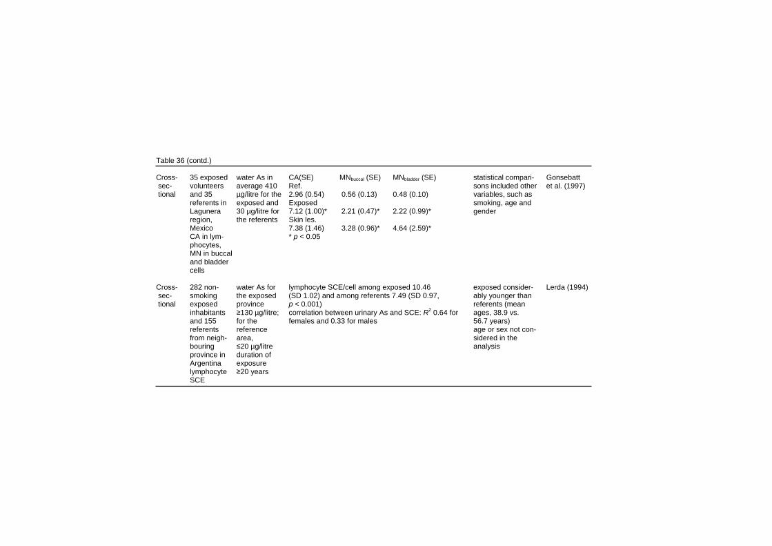
Table 36 (contd.) Cross- 35 exposed water As in CA(SE) MNbuccal (SE) MNbladder (SE) statistical compari- Gonsebatt sec- volunteers average 410 Ref. sons included other et al. (1997) tional and 35 µg/litre for the 2.96 (0.54) 0.56 (0.13) 0.48 (0.10) variables, such as referents in exposed and Exposed smoking, age and Lagunera 30 µg/litre for 7.12 (1.00)* 2.21 (0.47)* 2.22 (0.99)* gender region, the referents Skin les. Mexico 7.38 (1.46) 3.28 (0.96)* 4.64 (2.59)* CA in lym- * p < 0.05 phocytes, MN in buccal and bladder cells Cross- 282 non- water As for lymphocyte SCE/cell among exposed 10.46 exposed consider- Lerda (1994) sec- smoking the exposed (SD 1.02) and among referents 7.49 (SD 0.97, ably younger than tional exposed province p < 0.001) referents (mean inhabitants ≥130 µg/litre; correlation between urinary As and SCE: R2 0.64 for ages, 38.9 vs. and 155 for the females and 0.33 for males 56.7 years) referents reference age or sex not con- from neigh- area, sidered in the bouring ≤20 µg/litre analysis province in duration of Argentina exposure lymphocyte ≥20 years SCE

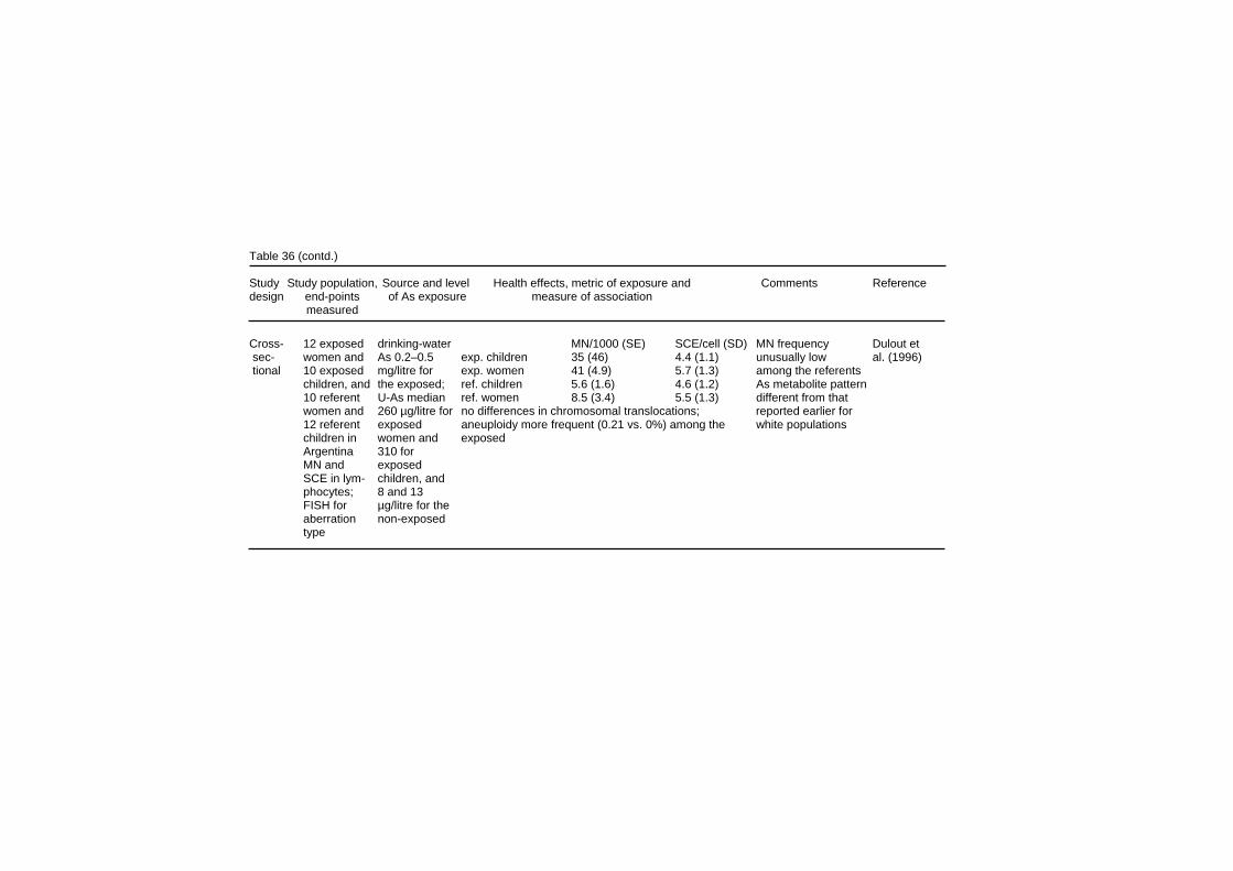
Table 36 (contd.) Study Study population, Source and level Health effects, metric of exposure and Comments Reference design end-points of As exposure measure of association measured Cross- 12 exposed drinking-water MN/1000 (SE) SCE/cell (SD) MN frequency Dulout et sec- women and As 0.2–0.5 exp. children 35 (46) 4.4 (1.1) unusually low al. (1996) tional 10 exposed mg/litre for exp. women 41 (4.9) 5.7 (1.3) among the referents children, and the exposed; ref. children 5.6 (1.6) 4.6 (1.2) As metabolite pattern 10 referent U-As median ref. women 8.5 (3.4) 5.5 (1.3) different from that women and 260 µg/litre for no differences in chromosomal translocations; reported earlier for 12 referent exposed aneuploidy more frequent (0.21 vs. 0%) among the white populations children in women and exposed Argentina 310 for MN and exposed SCE in lym- children, and phocytes; 8 and 13 FISH for µg/litre for the aberration non-exposed type

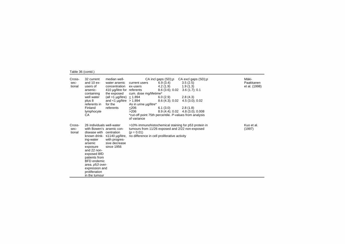
Table 36 (contd.) Cross- 32 current median well- CA incl gaps (SD);p CA excl gaps (SD);p Mäki- sec- and 10 ex- water arsenic current users 6.9 (3.4) 3.5 (2.5) Paakkanen tional users of concentration ex-users 4.2 (1.9) 1.9 (1.3) et al. (1998) arsenic- 410 µg/litre for referents 8.6 (3.6); 0.02 3.6 (1.7); 0.1 containing the exposed cum. dose mg/lifetime* well water (all >1 µg/litre) < 1.894 6.0 (2.9) 2.8 (4.3) plus 8 and <1 µg/litre > 1.894 8.6 (4.3); 0.02 4.5 (3.0); 0.02 referents in for the As in urine µg/litre* Finland referents <206 6.1 (3.0) 2.8 (1.8) lymphocyte >206 8.9 (4.4); 0.02 4.8 (3.0); 0.008 CA *cut-off point 75th percentile. P-values from analysis of variance Cross- 26 individuals well-water >10% immunohistochemical staining for p53 protein in Kuo et al. sec- with Bowen’s arsenic con- tumours from 11/26 exposed and 2/22 non-exposed (1997) tional disease with centration (p = 0.01) known drink- ≤1140 µg/litre, no difference in cell proliferative activity ing-water with progres- arsenic sive decrease exposure since 1956 and 22 non- exposed BfD patients from BFD endemic area. p53 over- expression and proliferation in the tumour

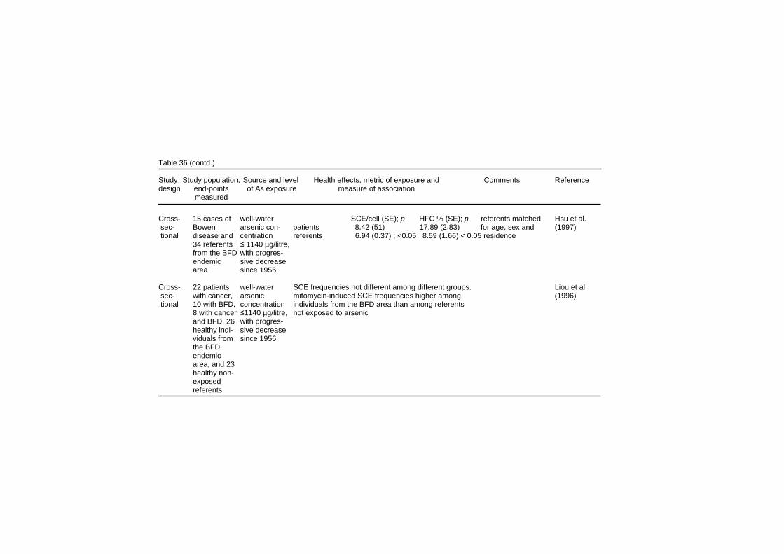
Table 36 (contd.) Study Study population, Source and level Health effects, metric of exposure and Comments Reference design end-points of As exposure measure of association measured Cross- 15 cases of well-water SCE/cell (SE); p HFC % (SE); p referents matched Hsu et al. sec- Bowen arsenic con- patients 8.42 (51) 17.89 (2.83) for age, sex and (1997) tional disease and centration referents 6.94 (0.37) ; <0.05 8.59 (1.66) < 0.05 residence 34 referents ≤ 1140 µg/litre, from the BFD with progres- endemic sive decrease area since 1956 Cross- 22 patients well-water SCE frequencies not different among different groups. Liou et al. sec- with cancer, arsenic mitomycin-induced SCE frequencies higher among (1996) tional 10 with BFD, concentration individuals from the BFD area than among referents 8 with cancer ≤1140 µg/litre, not exposed to arsenic and BFD, 26 with progres- healthy indi- sive decrease viduals from since 1956 the BFD endemic area, and 23 healthy non- exposed referents

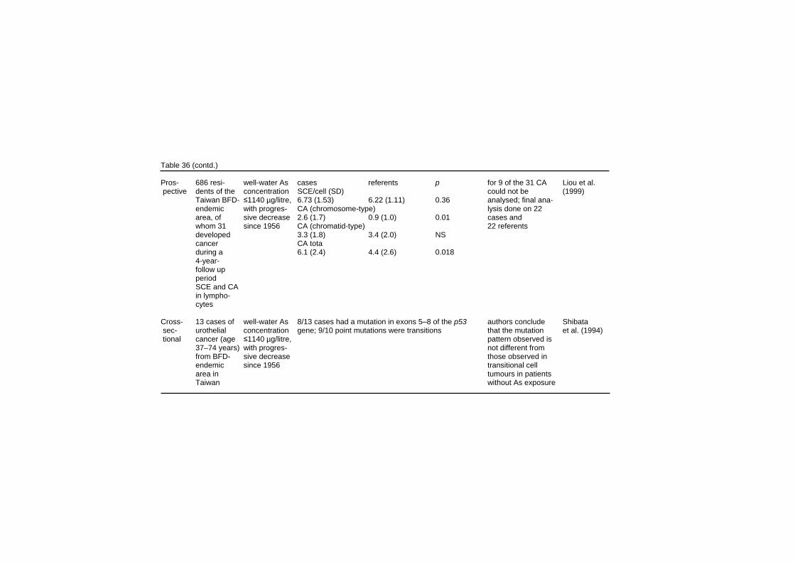
Table 36 (contd.) Pros- 686 resi- well-water As cases referents p for 9 of the 31 CA Liou et al. pective dents of the concentration SCE/cell (SD) could not be (1999) Taiwan BFD- ≤1140 µg/litre, 6.73 (1.53) 6.22 (1.11) 0.36 analysed; final ana- endemic with progres- CA (chromosome-type) lysis done on 22 area, of sive decrease 2.6 (1.7) 0.9 (1.0) 0.01 cases and whom 31 since 1956 CA (chromatid-type) 22 referents developed 3.3 (1.8) 3.4 (2.0) NS cancer CA tota during a 6.1 (2.4) 4.4 (2.6) 0.018 4-year- follow up period SCE and CA in lympho- cytes Cross- 13 cases of well-water As 8/13 cases had a mutation in exons 5–8 of the p53 authors conclude Shibata sec- urothelial concentration gene; 9/10 point mutations were transitions that the mutation et al. (1994) tional cancer (age ≤1140 µg/litre, pattern observed is 37–74 years) with progres- not different from from BFD- sive decrease those observed in endemic since 1956 transitional cell area in tumours in patients Taiwan without As exposure

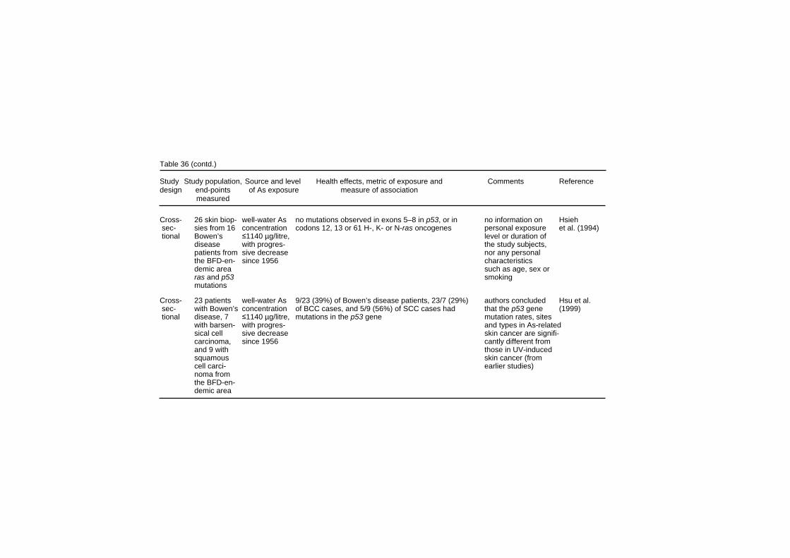
Table 36 (contd.) Study Study population, Source and level Health effects, metric of exposure and Comments Reference design end-points of As exposure measure of association measured Cross- 26 skin biop- well-water As no mutations observed in exons 5–8 in p53, or in no information on Hsieh sec- sies from 16 concentration codons 12, 13 or 61 H-, K- or N-ras oncogenes personal exposure et al. (1994) tional Bowen’s ≤1140 µg/litre, level or duration of disease with progres- the study subjects, patients from sive decrease nor any personal the BFD-en- since 1956 characteristics demic area such as age, sex or ras and p53 smoking mutations Cross- 23 patients well-water As 9/23 (39%) of Bowen’s disease patients, 23/7 (29%) authors concluded Hsu et al. sec- with Bowen’s concentration of BCC cases, and 5/9 (56%) of SCC cases had that the p53 gene (1999) tional disease, 7 ≤1140 µg/litre, mutations in the p53 gene mutation rates, sites with barsen- with progres- and types in As-related sical cell sive decrease skin cancer are signifi- carcinoma, since 1956 cantly different from and 9 with those in UV-induced squamous skin cancer (from cell carci- earlier studies) noma from the BFD-en- demic area

Effects on Humans In a larger study, differences in the frequency of bladder cell MN were investigated in volunteers from two northern Chilean communities with contrasting arsenic levels in drinking-water (Moore et al., 1997b). Bladder cell MN frequencies were higher in exposed men, and the difference increased when the analyses excluded individuals from the low exposure area with higher than background urinary arsenic levels (> 50 µg As/litre) (ratio = 2.0, 95% CI 1.3–3.1, p < 0.001). Smoking status did not affect the results. The prevalence of centromere positive cells was twice as high for the high-exposure group as for the modified low-exposure group (p = 0.02). Similar findings were reported for centromere-negative cells (1.2/1000) vs. 0.2/1000, p = 0.001). The increase in the centromere-negative cells in the high-exposure group indicates an increase in the proportion of chromosomal breakage vs. chromosomal lagging. The prevalence of MN increased from with exposure in exposure quintiles 1–4 (p for trend < 0.001). In the highest quintile, MN frequency returned to baseline, suggesting that MN formation may be inhibited at high doses owing to cytotoxicity or cytostasis. An intervention study was conducted as an extension of the work described above (Moore et al., 1997b). A selected group of families from the high-exposed town were provided with water lower in arsenic (45 µg/litre) for 2 months (Moore et al., 1997c). Overall, MN frequency among smokers (but not among non-smokers) decreased, but for men originally in the highest quintile of exposure there was an increase in the MN frequency, which was attributed to a decrease in cytotoxicity. Ostrosky-Wegman et al. (1991) compared various markers of effect in peripheral lymphocytes from individuals with high exposure and low exposure to arsenic in drinking-water in the Lagunera region of Mexico. There was no significant difference between the two groups in the rate of chromosomal aberrations, or SCEs. However, the average frequency of complex chromosomal aberrations (Cas; chromosome exchanges) was greater in the high-exposure group. There was also a slowdown in lymphocyte proliferation in the high-exposure group, indicating an alteration in the immune response. The HGPRT locus assay indicated that arsenic did not induce gene mutations.

341

EHC 224: Arsenic and Arsenic Compounds The effects of chronic arsenic exposure on lymphocyte proliferation were further investigated in a larger group from the same Lagunera region of Mexico (Gonsebatt et al., 1994). Blood and urine samples were obtained from exposed and unexposed adult residents from towns with different water arsenic levels. Exposure was assessed by questionnaires, and by urinary and water arsenic levels. Lymphocyte proliferation was performed at different culture times using labelling indexes (LI), mitotic indexes (MI) and replication indexes (RI). The results showed slower cell kinetics among exposed individuals overall, but variations in sub-groups were observed: mean LIs were higher among those with skin lesions, RIs were lower in exposed individuals, but this effect was significant only in females. No effects were found when correlating LIs, MIs or RIs with respect to age, duration of residence or urinary arsenic concentrations. In a subsequent study in the same area, Gonsebatt et al. (1997) examined the rates and types of CAs in lymphocytes, and the MN frequency in exfoliated buccal and bladder cells, in volunteers from the same towns (there is significant overlap of study subjects with Gonsebatt et al., 1994). In lymphocytes, the CA per cell, and the percentage of cells with CA, were higher in the exposed group than in the controls. The most frequent types of CA observed were chromatid deletions. The mean frequency of MN/1000 cells was also higher in the exposed group than in the control group, for both buccal cells and urothelial cells. Exposed individuals bearing skin lesions had higher frequencies of MN, but not CAs, than those without lesions. A study in Argentina examined the frequency of SCEs in relation to water and urinary arsenic levels of arsenic-exposed and unexposed persons (Lerda, 1994). Among the exposed, hyper-keratosis, melanosis, and basal carcinomas were observed. Water samples were obtained from each subject’s home and analysed for arsenic content. The mean SCE frequency was higher in the exposed than in the unexposed group. It should be noted that the control group was on average younger than the exposed group. The frequency of SCEs was not correlated with age, sex, or exposure to pesticides, lead, or other metals. The clastogenic and aneugenic potential for arsenic exposure, not contaminated with lead, cadmium, industrial pollution, or

342

Effects on Humans pesticides, was investigated in cultured lymphocytes from women and children from populations exposed to high arsenic levels from drinking-water in north-western Argentina (Dulout et al., 1996). The frequency of MN in lymphocytes from the exposed group was substantially higher than from the control group, both in children and in women. No differences were found for SCEs or for cell cycle progression analysis in relation to exposure level. The analysis of CAs indicated no differences in chromosomal translocations, but the frequency of numerical aberrations (aneuploidy–trisomy) was higher in the exposed group as supported by FISH analysis. The authors note that this population displays some unique characteristics which may be associated with distinct polymorphisms, since the frequency of MN in the low-exposure groups were about half of those previously reported for whites. In addition, patterns of urinary arsenic metabolites appear to be different than those of other studied populations. In a study conducted in Finland, individuals exposed to arsenic from well-water were compared to unexposed controls, with respect to urinary arsenic and frequency of CAs (Mäki-Paakkanen et al., 1998) Exposed subjects were classified as current users and ex-users of arsenic-laden water; the latter group had stopped using their well-water 2–4 months before the study began and were drinking from a low-arsenic source. The non-exposed group had the highest CA frequency, followed by current users and ex-users. However, when dichotomized into two urinary arsenic concentration or cumulative lifetime exposure groups, CAs were highest in the high-exposure group. When urinary arsenic was entered as a continuous variable in a regression model (adjusting for gender, age, smoking and cell culture batch), the correlation was stronger for CA excluding gaps (all subjects r = 0.23, p = 0.02; current users r = 0.30, p = 0.06). A comparative investigation assessed the activity of the p53 gene in formalin-fixed biopsy samples from 48 individuals diagnosed with Bowen’s disease with (n = 26) or without (n = 22) a history of exposure to arsenic (Kuo et al., 1997). The rates of p53 positivity were higher in the arsenic-exposed group. In a sub-group of 5 cases which had multiple lesions examined, the p53 status remained 100% consistent within individuals, adding strength to the association. The p53 overexpression did not seem linked to the proliferative activity.

343

EHC 224: Arsenic and Arsenic Compounds Patients with Bowen’s disease in the BFD-endemic area in Taiwan were found to have a higher frequency of SCEs and HFCs and a lower RI (Hsu et al., 1997). In vitro treatment with sodium arsenite increased SCEs, HFCs and RI, but only the decrease in RI was statistically more pronounced in arsenic-induced Bowen’s disease patients than controls. Liou et al. (1996) also examined the rates of SCEs and mitomycin C-induced SCEs in patients with cancer only (17 skin, 5 other types), BFD only, with both BFD and cancer (6 with skin cancer), and healthy controls from the BFD area. In addition, healthy non-arsenic-exposed workers were used as external controls. The baseline SCEs did not differ among the 5 groups studied. Although smokers consistently had higher SCEs than non-smokers across all groups, no differences were observed between groups when stratified by smoking status. After in vitro treatment with mitomycin, the increase in SCEs was the same in lymphocytes from the 4 BFD-area groups (among which there were no differences in lifetime exposure to arsenic in well-water), but they were overall higher than in the external controls. A nested case–control study was performed in the BFD-endemic area of Taiwan (Liou et al., 1999). A cohort of 686 residents was assembled, and after 4 years, 31 people had developed cancer. Of these, blood samples obtained at the beginning of the cohort study were successfully processed for 22 cases. Controls were selected from among members of the cohort who had not developed cancer, matched on sex, age, village of residence and smoking. No differences were found in overall frequencies of SCEs. The frequency of total CAs was significantly higher among the cases. When categorized by specific type of CA, all chromosome-type CAs were significant except exchanges, whereas none of the chromatid-type CAs were significant. The limitation of this investigation is the apparent uniformity of arsenic exposure among cases and controls, making it hard to link the CA frequency with arsenic, rather than to other factors, or genetic susceptibility. An investigation focused on p53 analysis was performed on 13 urothelial tumours from residents of the BFD area in Taiwan (Shibata et al., 1994); 11 cases were transitional cell carcinomas and 2 were squamous cell carcinomas. DNA was extracted from archival

344

Effects on Humans tissue and analysed for mutations in the p53 gene by SSCP, and if mutations were identified, these were subsequently sequenced. Eight cases (62%) showed mutations and 9 of the 10 point mutations observed were transitions. The type of mutations was not different from the p53 mutational spectra of other transitional cell carcinomas. However, 2 of the mutations were at a mutational hot spot for colon cancer, but not previously associated with transitional cell carcinomas except in cases associated with inflammatory agents (e.g. phenacetin, schistosomiasis); and 3 of the tumours contained double mutations, a relatively rare mutagenic event in human cancers. Hsieh et al. (1994) examined 26 skin biopsies from 16 patients from the BFD-endemic area of Taiwan with arsenic-related Bowen’s disease, looking for p53 mutations by SSCP on exons 5–8, and for mutations of H-, K-, and N-ras genes. No mutations were detected in any of the samples analysed. These results are contrary to what is found in UV-related skin tumours, where mutations in all the genes studied have been detected. To understand the role of the p53 gene in the process of carcinogenesis of arsenic-induced skin cancers, samples of tumour specimens and normal skin were collected from 23 patients with Bowen’s disease, 7 with basal cell carcinomas and 9 with squamous cell carcinoma (Hsu et al., 1999). All the tumours were from patients from the BFD-endemic area in Taiwan, and were collected from areas of the body not usually exposed to sunlight. Direct sequencing of the p53 gene on exons 2–11 showed six types of p53 mutations, with 38% of the type G:C A:T transition, as well as the finding of the same hot spot in 3 cases (codon 175). The frequency of p53 mutations differed by tumour type, although the groups were quite small: 39% of Bowen’s disease cases, 29% of basal cell carcinoma cases, and 56% of squamous cell carcinoma cases. Overall, the p53 gene mutation rates, sites and types in arsenic-related skin cancer were significantly different from those in UV-induced skin cancer.

345

iii

LINKS TO THE OTHER SECTIONS OF THE DOCUMENT PREAMBLE ABBREVIATIONS SUMMARY, RESUME, RESUMEN PROPERTIES AND ANALYTICAL PROCEDURES SOURCES AND OCCURRENCE OF ARSENIC IN THE ENVIRONMENT ENVIRONMENTAL TRANSPORT AND DISTRIBUTION ENVIRONMENTAL LEVELS AND HUMAN EXPOSURE KINETICS AND METABOLISM IN LABORATORY ANIMALS AND HUMANS EFFECTS ON LABORATORY MAMMALS AND IN VITRO TEST SYSTEMS EFFECTS ON OTHER ORGANISMS IN THE ENVIRONMENT EVALUATION OF HUMAN HEALTH RISKS AND EFFECTS ON THE ENVIRONMENT RECOMMENDATIONS FOR FUTURE RESEARCH PREVIOUS EVALUATIONS BY INTERNATIONAL BODIES REFERENCES