Embed Size (px)
Citation preview
8 - 1
Financial options
Black-Scholes Option Pricing Model
CHAPTER 8Financial Options and Their Valuation
8 - 2
An option is a contract which gives its holder the right, but not the obligation, to buy (or sell) an asset at some predetermined price within a specified period of time.
What is a financial option?
8 - 3
It does not obligate its owner to take any action. It merely gives the owner the right to buy or sell an asset.
What is the single most importantcharacteristic of an option?
8 - 4
Call option: An option to buy a specified number of shares of a security within some future period.
Put option: An option to sell a specified number of shares of a security within some future period.
Exercise (or strike) price: The price stated in the option contract at which the security can be bought or sold.
Option Terminology
8 - 5
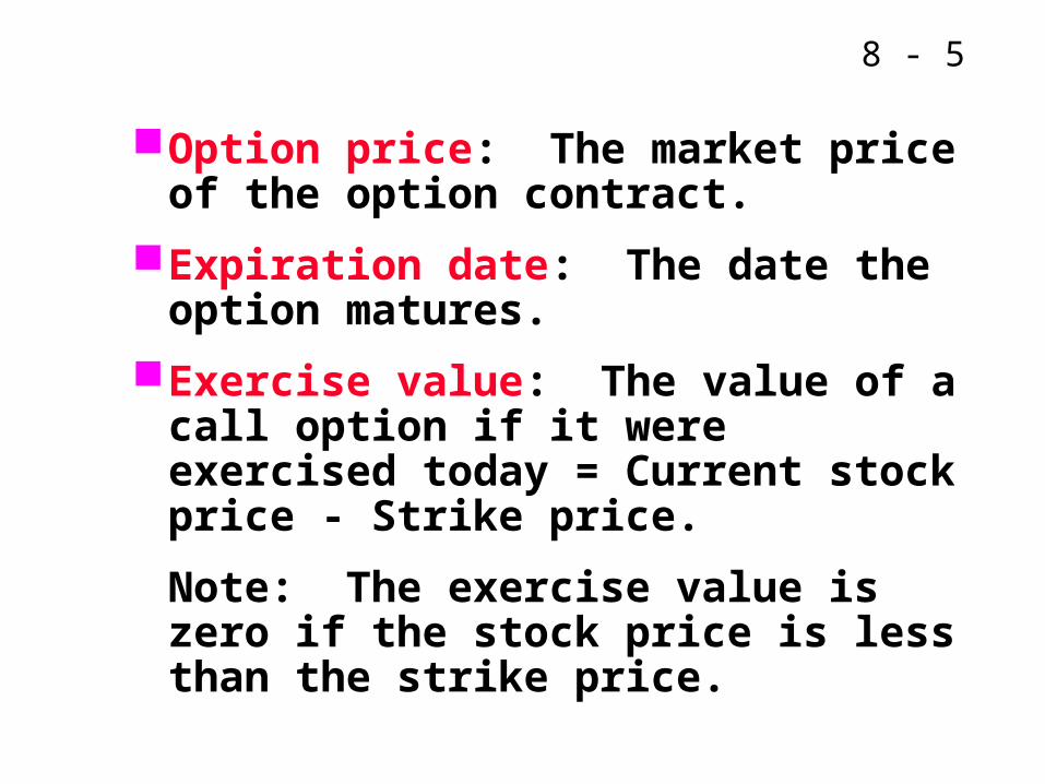
Option price: The market price of the option contract.
Expiration date: The date the option matures.
Exercise value: The value of a call option if it were exercised today = Current stock price - Strike price.
Note: The exercise value is zero if the stock price is less than the strike price.
8 - 6
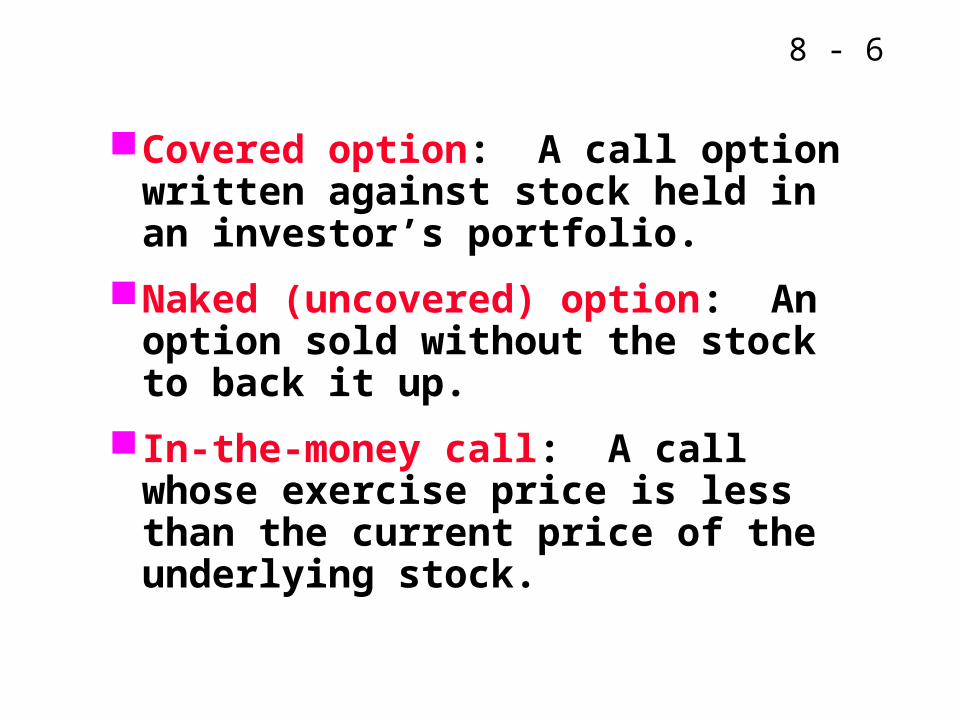
Covered option: A call option written against stock held in an investor’s portfolio.
Naked (uncovered) option: An option sold without the stock to back it up.
In-the-money call: A call whose exercise price is less than the current price of the underlying stock.
8 - 7
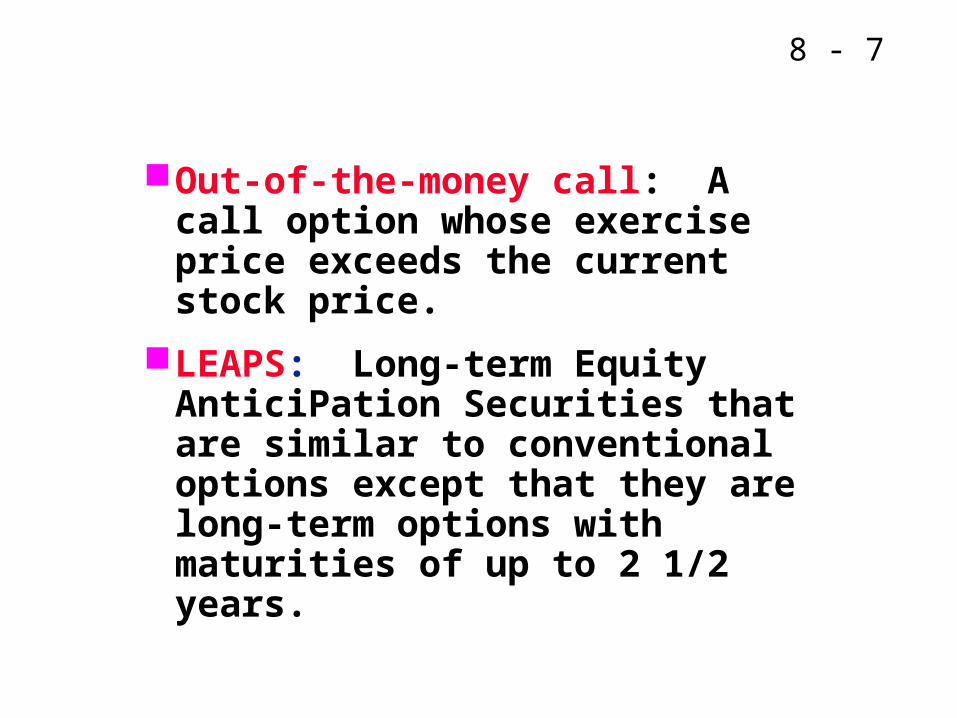
Out-of-the-money call: A call option whose exercise price exceeds the current stock price.
LEAPS: Long-term Equity AnticiPation Securities that are similar to conventional options except that they are long-term options with maturities of up to 2 1/2 years.
8 - 8
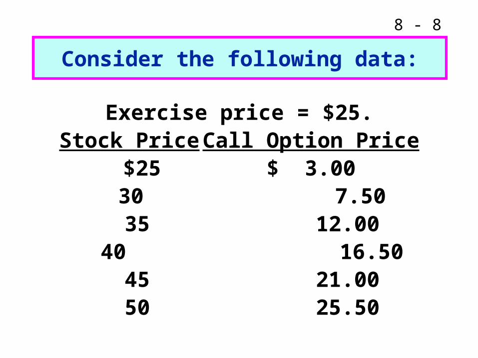
Exercise price = $25.Stock Price Call Option Price
$25 $ 3.00 30 7.50 35 12.00 40 16.50 45 21.00 50 25.50
Consider the following data:
8 - 9
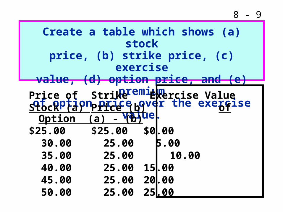
Create a table which shows (a) stockprice, (b) strike price, (c) exercise
value, (d) option price, and (e) premiumof option price over the exercise value.
Price of Strike Exercise ValueStock (a) Price (b) of Option (a) - (b)$25.00 $25.00 $0.00 30.00 25.00 5.00 35.00 25.00 10.00 40.00 25.00 15.00 45.00 25.00 20.00 50.00 25.00 25.00
8 - 10
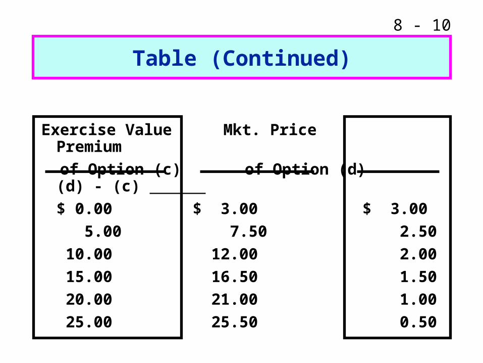
Exercise Value Mkt. Price Premium
of Option (c) of Option (d) (d) - (c)
$ 0.00 $ 3.00 $ 3.00
5.00 7.50 2.50
10.00 12.00 2.00
15.00 16.50 1.50
20.00 21.00 1.00
25.00 25.50 0.50
Table (Continued)
8 - 11
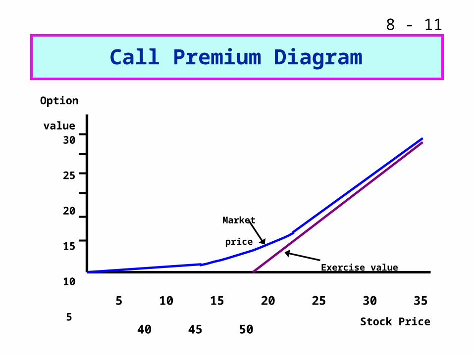
Call Premium Diagram
5 10 15 20 25 30 35 40 45 50
Stock Price
Option value
30
25
20
15
10
5
Market price
Exercise value
8 - 12
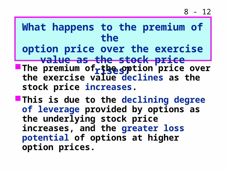
What happens to the premium of the option price over the exercisevalue as the stock price rises?
The premium of the option price over the exercise value declines as the stock price increases.
This is due to the declining degree of leverage provided by options as the underlying stock price increases, and the greater loss potential of options at higher option prices.
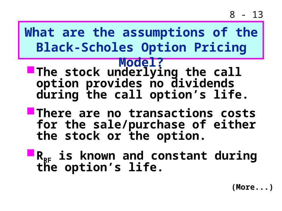
8 - 13
The stock underlying the call option provides no dividends during the call option’s life.
There are no transactions costs for the sale/purchase of either the stock or the option.
RRF is known and constant during the option’s life.
What are the assumptions of theBlack-Scholes Option Pricing Model?
(More...)
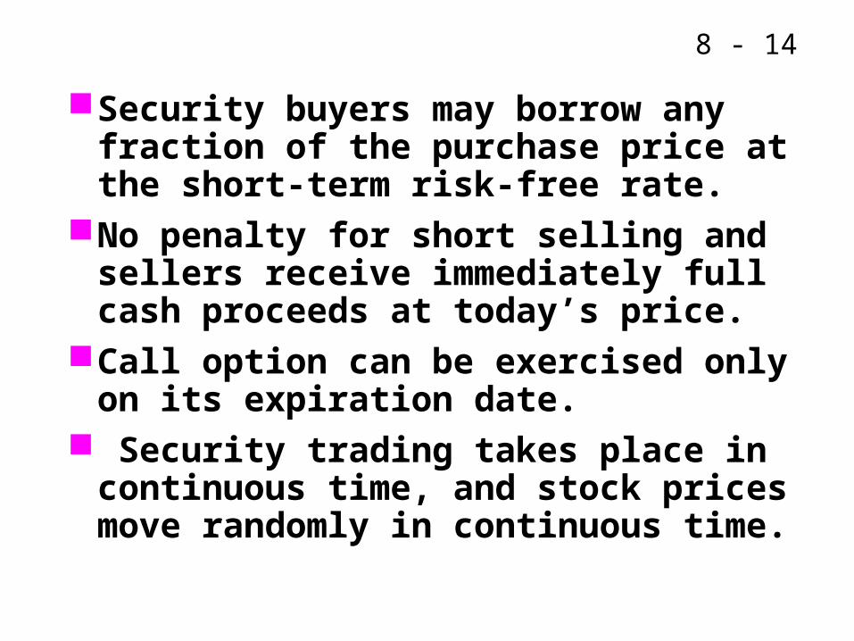
8 - 14
Security buyers may borrow any fraction of the purchase price at the short-term risk-free rate.
No penalty for short selling and sellers receive immediately full cash proceeds at today’s price.
Call option can be exercised only on its expiration date.
Security trading takes place in continuous time, and stock prices move randomly in continuous time.
8 - 15
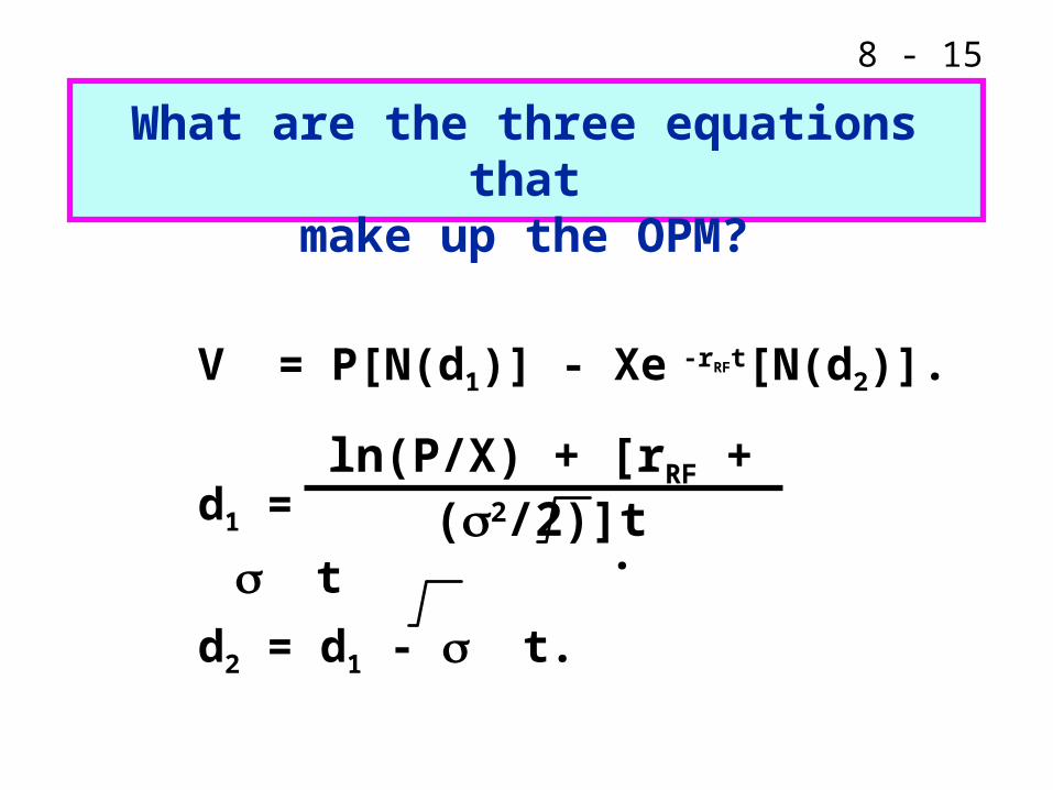
V = P[N(d1)] - Xe -rRFt[N(d2)].
d1 = . t
d2 = d1 - t.
What are the three equations thatmake up the OPM?
ln(P/X) + [rRF + (2/2)]t
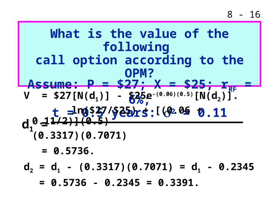
8 - 16
What is the value of the following call option according to the OPM?Assume: P = $27; X = $25; rRF = 6%;
t = 0.5 years: 2 = 0.11
V = $27[N(d1)] - $25e-(0.06)(0.5)[N(d2)].
ln($27/$25) + [(0.06 + 0.11/2)](0.5)
(0.3317)(0.7071)
= 0.5736.
d2 = d1 - (0.3317)(0.7071) = d1 - 0.2345
= 0.5736 - 0.2345 = 0.3391.
d1 =
8 - 17
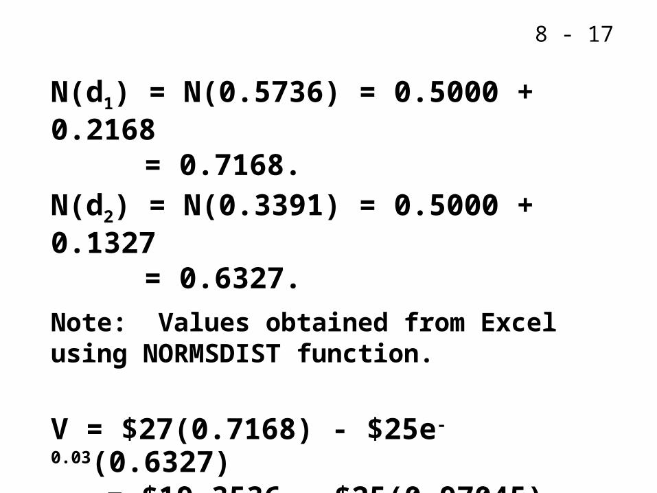
N(d1) = N(0.5736) = 0.5000 + 0.2168 = 0.7168.
N(d2) = N(0.3391) = 0.5000 + 0.1327 = 0.6327.
Note: Values obtained from Excel using NORMSDIST function.
V = $27(0.7168) - $25e-0.03(0.6327) = $19.3536 - $25(0.97045)(0.6327) = $4.0036.
8 - 18
Current stock price: Call option value increases as the current stock price increases.
Exercise price: As the exercise price increases, a call option’s value decreases.
What impact do the following para-meters have on a call option’s value?
8 - 19
Option period: As the expiration date is lengthened, a call option’s value increases (more chance of becoming in the money.)
Risk-free rate: Call option’s value tends to increase as rRF increases (reduces the PV of the exercise price).
Stock return variance: Option value increases with variance of the underlying stock (more chance of becoming in the money).
8 - 20
Put-Call Parity
Portfolio 1:
Put option,
Share of stock, P
Portfolio 2:
Call option, V
PV of exercise price, X
8 - 21
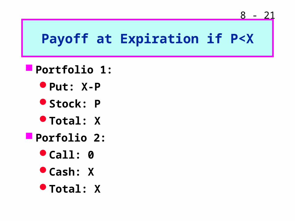
Payoff at Expiration if P<X
Portfolio 1:
Put: X-P
Stock: P
Total: X
Porfolio 2:
Call: 0
Cash: X
Total: X
8 - 22
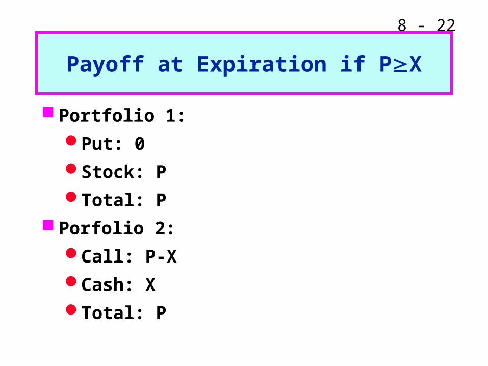
Payoff at Expiration if PX
Portfolio 1:
Put: 0
Stock: P
Total: P
Porfolio 2:
Call: P-X
Cash: X
Total: P
8 - 23
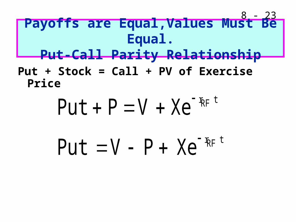
Payoffs are Equal,Values Must Be Equal.Put-Call Parity Relationship
Put + Stock = Call + PV of Exercise Price
tRFr
tRFr
XePVPut
XeVPPut
8 - 24
Real options
Decision trees
Application of financial options to real options
CHAPTER 12 Real Options
8 - 25
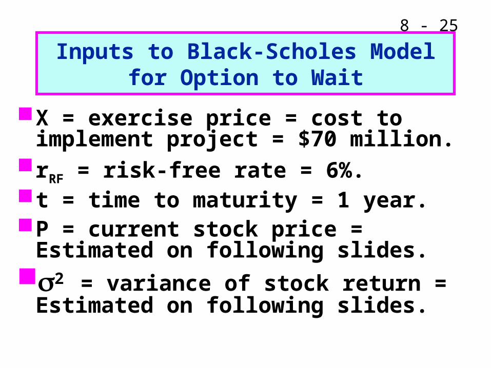
Inputs to Black-Scholes Model for Option to Wait
X = exercise price = cost to implement project = $70 million.
rRF = risk-free rate = 6%.t = time to maturity = 1 year.P = current stock price = Estimated on
following slides. 2 = variance of stock return =
Estimated on following slides.
8 - 26
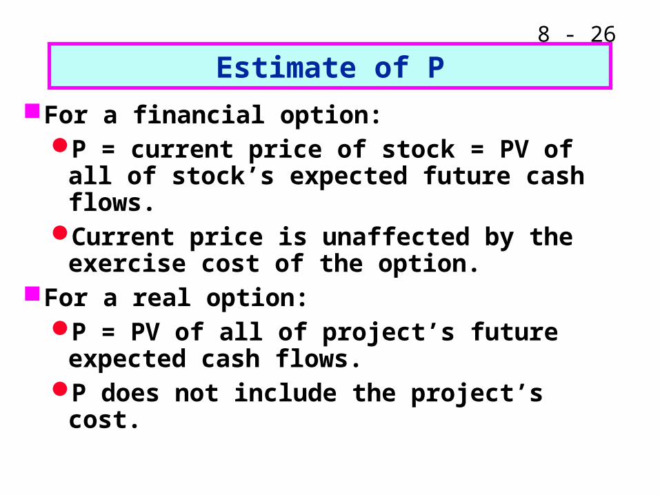
Estimate of P
For a financial option:P = current price of stock = PV of all
of stock’s expected future cash flows.Current price is unaffected by the
exercise cost of the option.For a real option:
P = PV of all of project’s future expected cash flows.
P does not include the project’s cost.
8 - 27
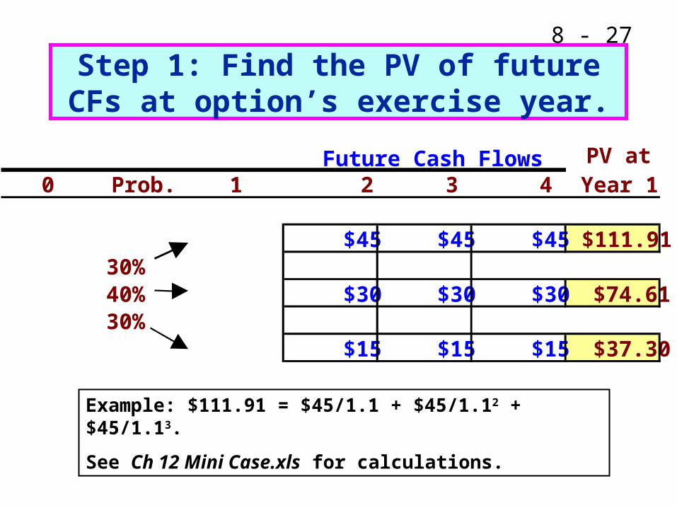
Step 1: Find the PV of future CFs at option’s exercise year.
PV at 0 Prob. 1 2 3 4 Year 1
$45 $45 $45 $111.9130%40% $30 $30 $30 $74.6130%
$15 $15 $15 $37.30
Future Cash Flows
Example: $111.91 = $45/1.1 + $45/1.12 + $45/1.13.
See Ch 12 Mini Case.xls for calculations.
8 - 28
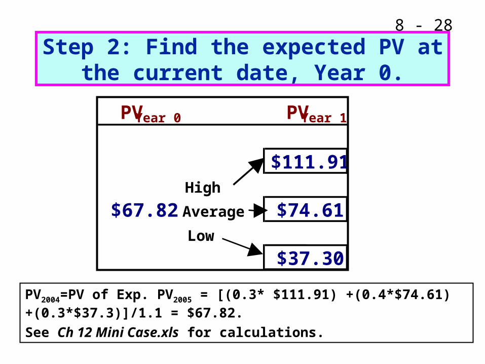
Step 2: Find the expected PV at the current date, Year 0.
PV2004=PV of Exp. PV2005 = [(0.3* $111.91) +(0.4*$74.61) +(0.3*$37.3)]/1.1 = $67.82.
See Ch 12 Mini Case.xls for calculations.
PVYear 0 PVYear 1
$111.91High
$67.82 Average $74.61Low
$37.30
8 - 29
The Input for P in the Black-Scholes Model
The input for price is the present value of the project’s expected future cash flows.
Based on the previous slides,
P = $67.82.
8 - 30
Estimating 2 for the Black-Scholes Model
For a financial option, 2 is the variance of the stock’s rate of return.
For a real option, 2 is the variance of the project’s rate of return.
8 - 31
Three Ways to Estimate 2
Judgment.
The direct approach, using the results from the scenarios.
The indirect approach, using the expected distribution of the project’s value.
8 - 32
Estimating 2 with Judgment
The typical stock has 2 of about 12%.
A project should be riskier than the firm as a whole, since the firm is a portfolio of projects.
The company in this example has 2 = 10%, so we might expect the project to have 2 between 12% and 19%.
8 - 33
Estimating 2 with the Direct Approach
Use the previous scenario analysis to estimate the return from the present until the option must be exercised. Do this for each scenario
Find the variance of these returns, given the probability of each scenario.
8 - 34
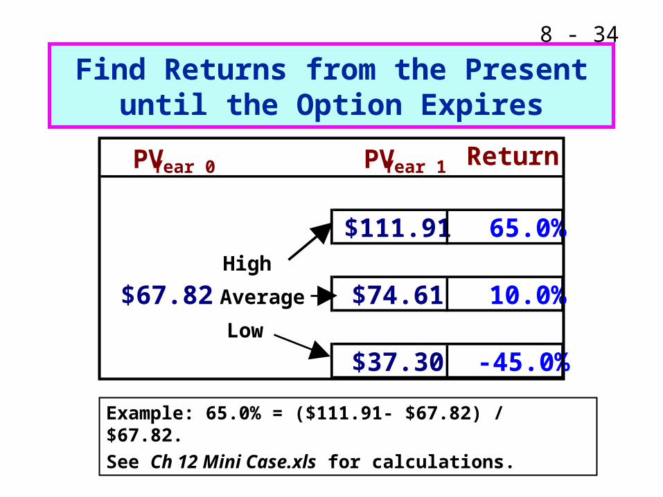
Find Returns from the Present until the Option Expires
Example: 65.0% = ($111.91- $67.82) / $67.82.
See Ch 12 Mini Case.xls for calculations.
PVYear 0 PVYear 1 Return
$111.91 65.0%High
$67.82 Average $74.61 10.0%Low
$37.30 -45.0%
8 - 35
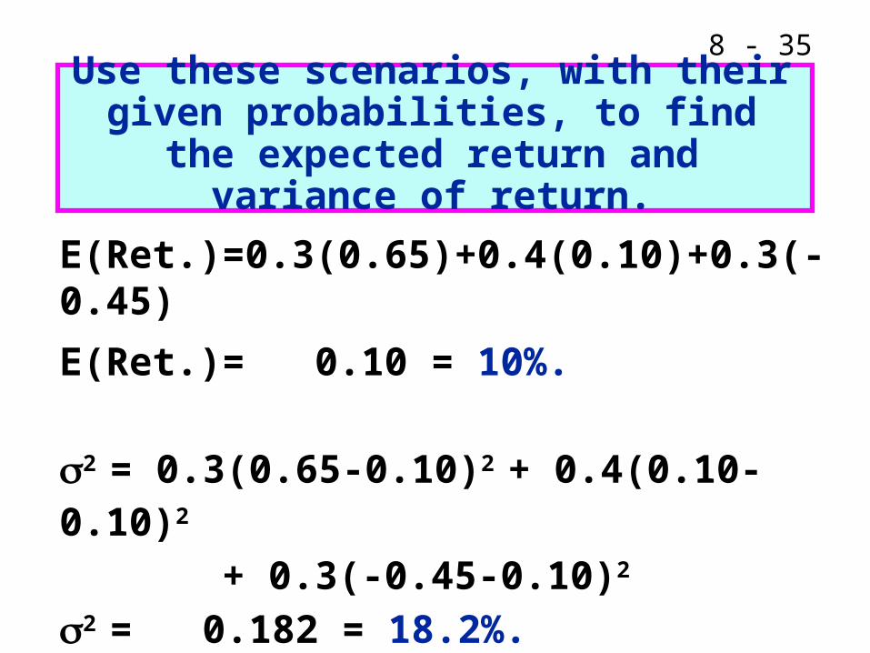
E(Ret.)=0.3(0.65)+0.4(0.10)+0.3(-0.45)
E(Ret.)= 0.10 = 10%.
2 = 0.3(0.65-0.10)2 + 0.4(0.10-0.10)2
+ 0.3(-0.45-0.10)2
2 = 0.182 = 18.2%.
Use these scenarios, with their given probabilities, to find the expected
return and variance of return.
8 - 36
Estimating 2 with the Indirect Approach
From the scenario analysis, we know the project’s expected value and the variance of the project’s expected value at the time the option expires.
The questions is: “Given the current value of the project, how risky must its expected return be to generate the observed variance of the project’s value at the time the option expires?”
8 - 37
The Indirect Approach (Cont.)
From option pricing for financial options, we know the probability distribution for returns (it is lognormal).
This allows us to specify a variance of the rate of return that gives the variance of the project’s value at the time the option expires.
8 - 38
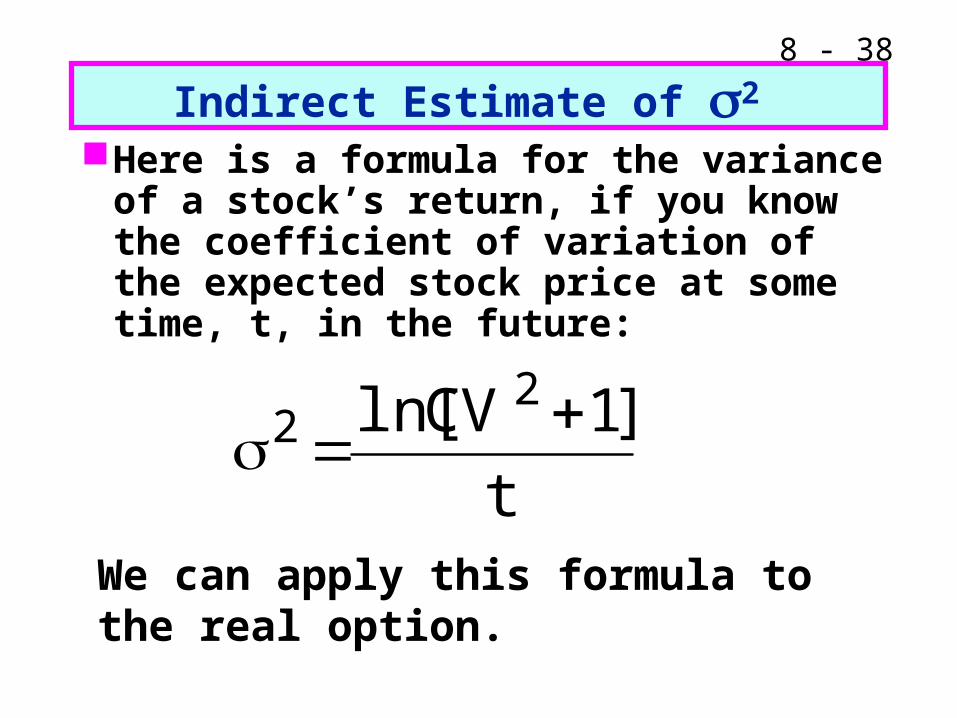
Indirect Estimate of 2 Here is a formula for the variance of a
stock’s return, if you know the coefficient of variation of the expected stock price at some time, t, in the future:
t
]1CVln[ 22
We can apply this formula to the real option.
8 - 39
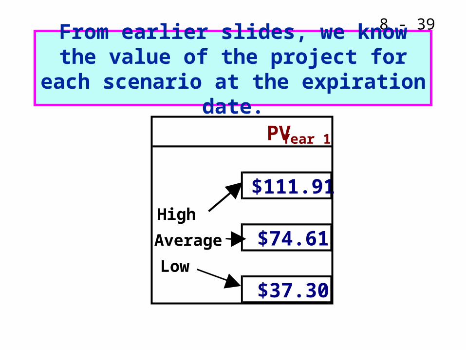
From earlier slides, we know the value of the project for each scenario at the
expiration date.
PVYear 1
$111.91High
Average $74.61Low
$37.30
8 - 40
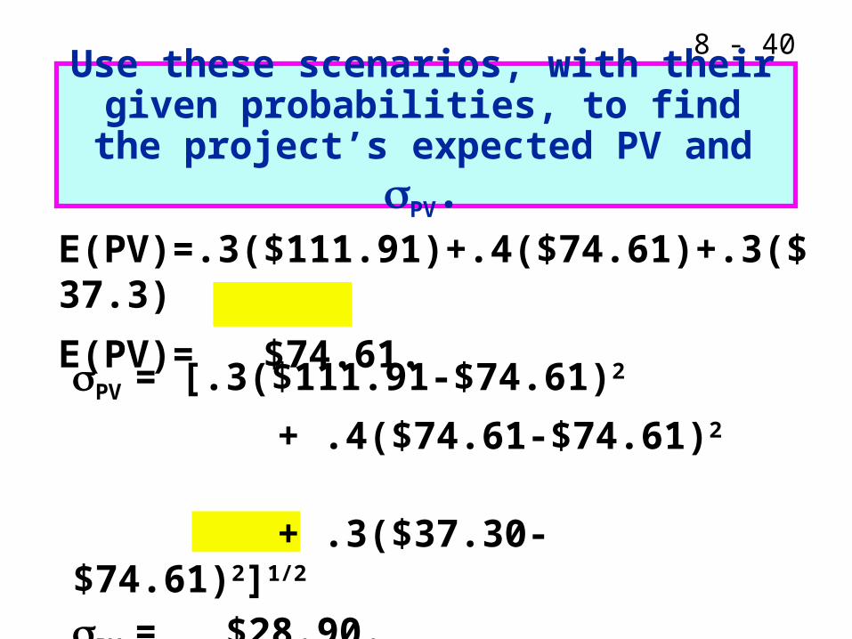
E(PV)=.3($111.91)+.4($74.61)+.3($37.3)
E(PV)= $74.61.
Use these scenarios, with their given probabilities, to find the project’s
expected PV and PV.
PV = [.3($111.91-$74.61)2
+ .4($74.61-$74.61)2 + .3($37.30-$74.61)2]1/2
PV = $28.90.
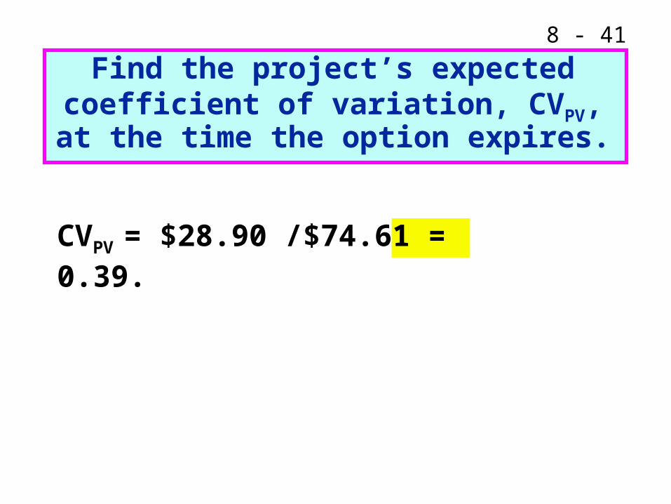
8 - 41
Find the project’s expected coefficient of variation, CVPV, at the time the option
expires.
CVPV = $28.90 /$74.61 = 0.39.
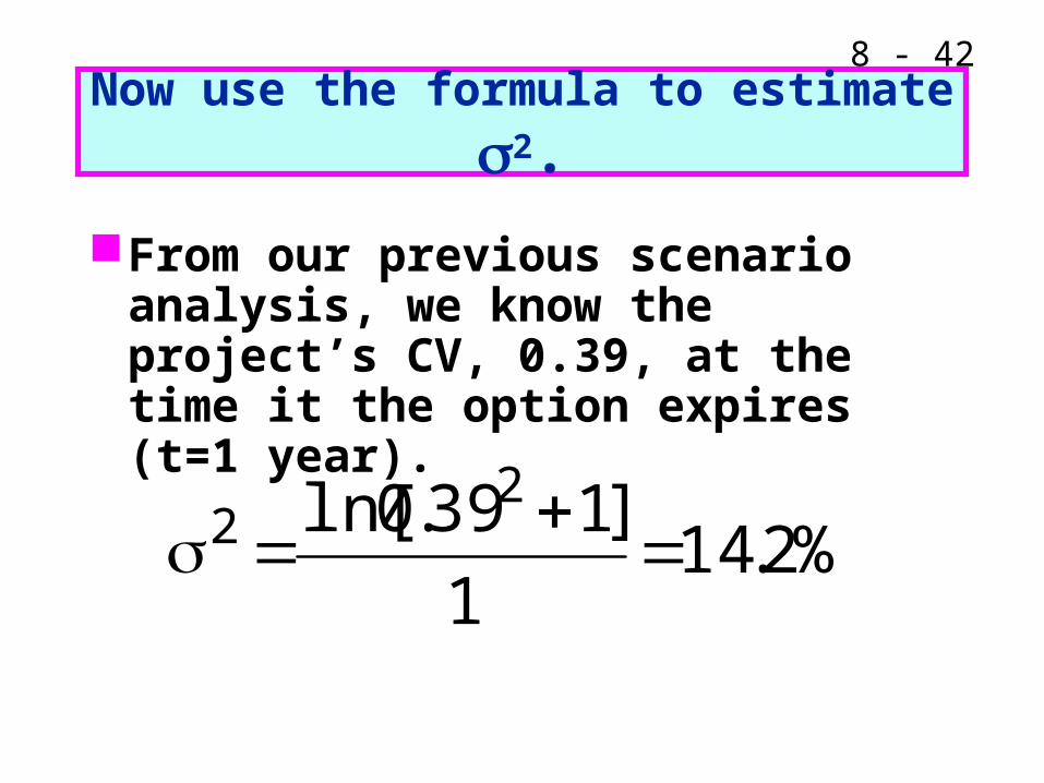
8 - 42
Now use the formula to estimate 2.
From our previous scenario analysis, we know the project’s CV, 0.39, at the time it the option expires (t=1 year).
%2.141
]139.0ln[ 22
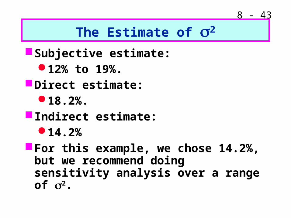
8 - 43
The Estimate of 2
Subjective estimate:12% to 19%.
Direct estimate:18.2%.
Indirect estimate:14.2%
For this example, we chose 14.2%, but we recommend doing sensitivity analysis over a range of 2.
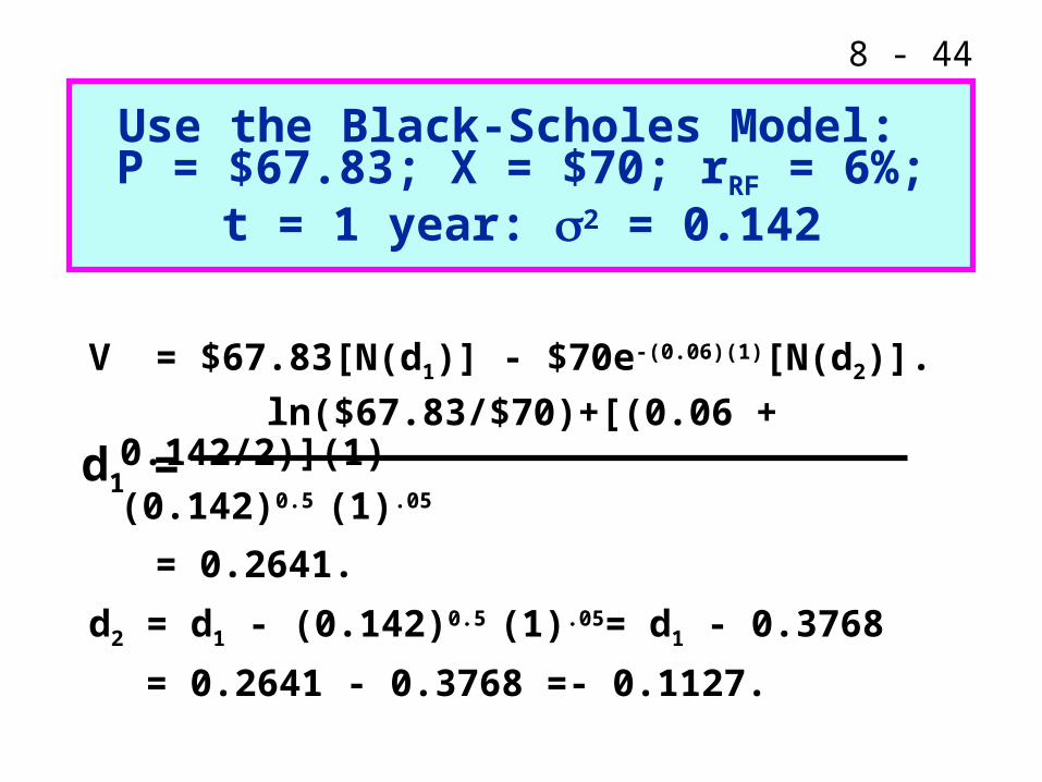
8 - 44
Use the Black-Scholes Model: P = $67.83; X = $70; rRF = 6%;
t = 1 year: 2 = 0.142
V = $67.83[N(d1)] - $70e-(0.06)(1)[N(d2)].
ln($67.83/$70)+[(0.06 + 0.142/2)](1)
(0.142)0.5 (1).05
= 0.2641.
d2 = d1 - (0.142)0.5 (1).05= d1 - 0.3768
= 0.2641 - 0.3768 =- 0.1127.
d1 =
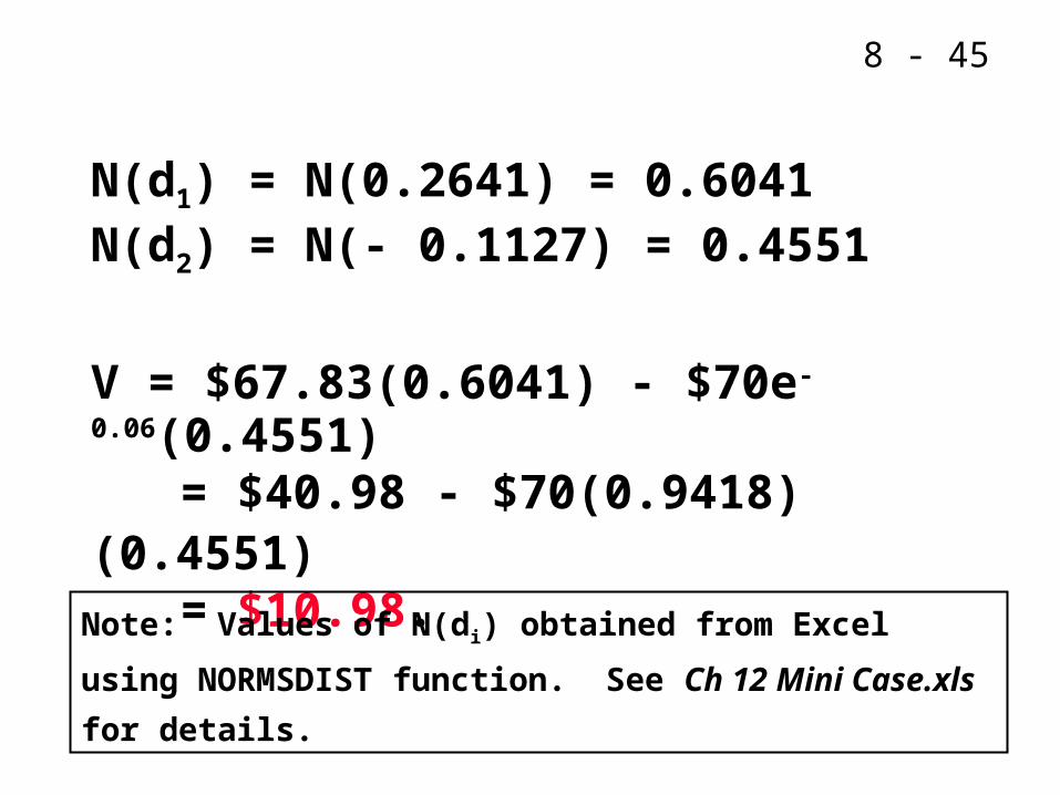
8 - 45
N(d1) = N(0.2641) = 0.6041N(d2) = N(- 0.1127) = 0.4551
V = $67.83(0.6041) - $70e-0.06(0.4551) = $40.98 - $70(0.9418)(0.4551) = $10.98.
Note: Values of N(di) obtained from Excel using
NORMSDIST function. See Ch 12 Mini Case.xls for details.
8 - 46
Real Options
8 - 47
Option Theory and Investment Decisions
Traditional investment analysis uses the NPV rule to decide on investment projects
The concept of net present value uses expected cash flows, discounted at a constant discount rate which is assumed to capture the risk of these cash flows
Making investment decisions based on a project’s NPV is equivalent to assuming that the firm’s managers have no ability to respond to uncertainty (no managerial flexibility)
8 - 48
Option Theory and Investment Decisions
Example: Suppose that a firm will invest $600m over the next two years ($250m this year and $350m next year) to build a new factory with a life of 20 years
Suppose that revenues from this factory will be $80m starting 3 years from now and grow at 8% annually and that the costs to run the factory will be $60m (also staring 3 years from now) and grow at 6%
Assume for simplicity that there are no working capital investments, no taxes, no salvage value, and that the firm will use straight-line depreciation starting two years from now
8 - 49
Option Theory and Investment Decisions
If the firm’s WACC is 10%, this project’s NPV is -$1.44m so we reject the project
The above analysis may fail to capture some aspects of the project
The initial investment takes place in stages and can be abandoned at each
If the project goes well, perhaps it can be expanded or extended
If it goes bad, perhaps it can be scaled back or sold at a floor price
Perhaps there is the option to delay building the factory for some time
8 - 50
Option Theory and Investment Decisions
Example: Suppose that you are given the choice to put $1 in a toy bank that guarantees $1.05 a year later with certainty
This offer is good for only one year
Alternatively, interest rates in a real bank are currently at 10%
How much is the toy bank offer worth?
8 - 51
Option Theory and Investment Decisions
Real options are options that give the right to make decisions on a capital investment project
Real options are American options
A limitation of traditional investment analysis is that it is static, meaning that it does not do a good job capturing the value of options embedded in a project
One can go as far as arguing that the NPV rule systematically undervalues every project
8 - 52
Option Theory and Investment Decisions
These options add value to a project and may change a project’s NPV from negative (under traditional analysis) into positive
Project’s value = NPV + Value of option
8 - 53
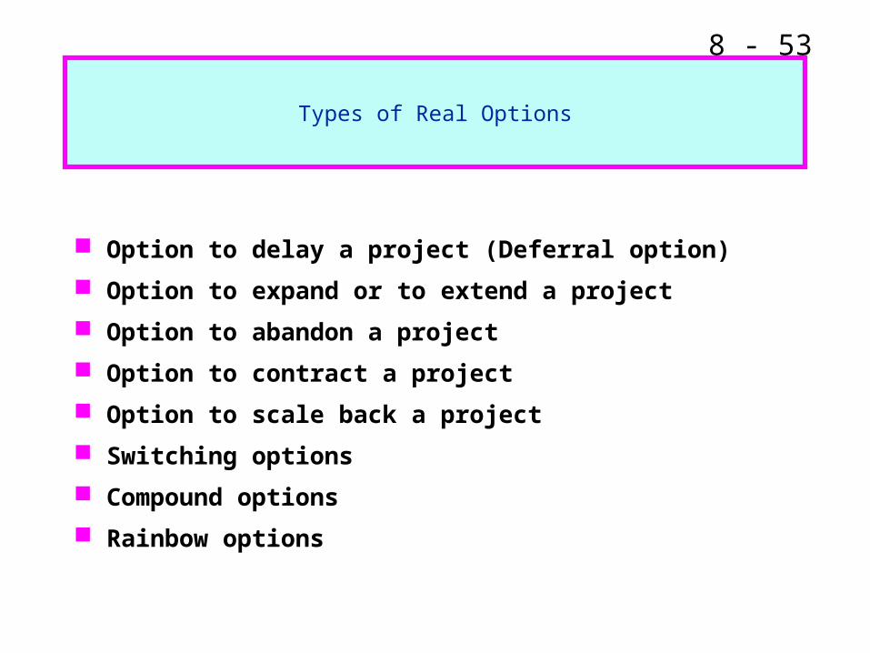
Types of Real Options
Option to delay a project (Deferral option)
Option to expand or to extend a project
Option to abandon a project
Option to contract a project
Option to scale back a project
Switching options
Compound options
Rainbow options
8 - 54
The Option to Delay a Project
If a firm has exclusive rights to a project or a product for a specific period, it can delay taking the project or introducing the product until a later date
A project that has a negative NPV today may have a positive NPV at some future date
The reason is that expected cash flows and the discount rate may change through time, meaning there are changes in the business environment
8 - 55
The Option to Delay a Project
This resembles a call option (deferral option) where
The underlying asset is the project
The strike price is the investment needed to take the project
The life of the option is the period that the firm can delay undertaking the project
The value of the option increases with the volatility in the business environment
8 - 56
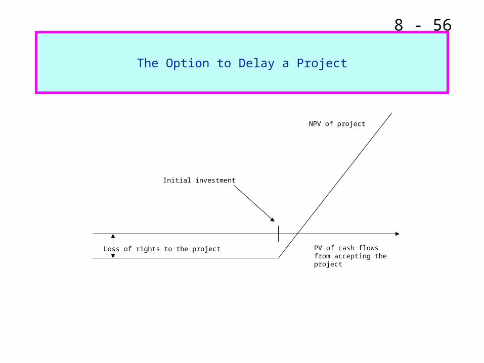
The Option to Delay a Project
NPV of project
PV of cash flowsfrom accepting theproject
Initial investment
Loss of rights to the project
8 - 57
The Option to Expand a Project or Take Other Projects
Taking a project today may allow a firm to expand the project or consider taking other projects in the future
The value of this option may change the NPV of a project
These call options are called strategic options
Example: Honda, Toyota, GM, Ford are investing in cars with hybrid engines, which, despite current losses, gives them the option to gain technological and production expertise to produce an eco-car profitably in the future
8 - 58
The Option to Abandon a Project
A firm may have the option to abandon a project if the cash flows from the project do not match the firm’s expectations
If abandoning the project allows the firm to save itself from further losses, then this put option increases the value of the project and makes it more attractive
Firms try to build such options in the contracts signed with other parties involved in a project
8 - 59
Other Types of Real Options
Switching Real Options are portfolios of call and put options that allow their owner to switch at a fixed cost between two modes of operation
Example: the option to shut down a manufacturing plant when demand is low and reopen it when demand picks up (General Motors assembly plants)
Compound real options are options on options typically found in phased investment projects
8 - 60
Other Types of Real Options
Example: The decision to build a chemical plant may involve three phases: a design phase, an engineering phase and construction
At each phase, the firm has the option to stop or defer the project
Thus, each phase is an option that depends on the earlier exercise of another option
Rainbow options are options driven by multiple sources of uncertainty (e.g., exploration and development)
8 - 61
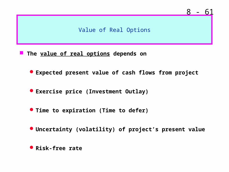
Value of Real Options
The value of real options depends on
Expected present value of cash flows from project
Exercise price (Investment Outlay)
Time to expiration (Time to defer)
Uncertainty (volatility) of project’s present value
Risk-free rate
8 - 62
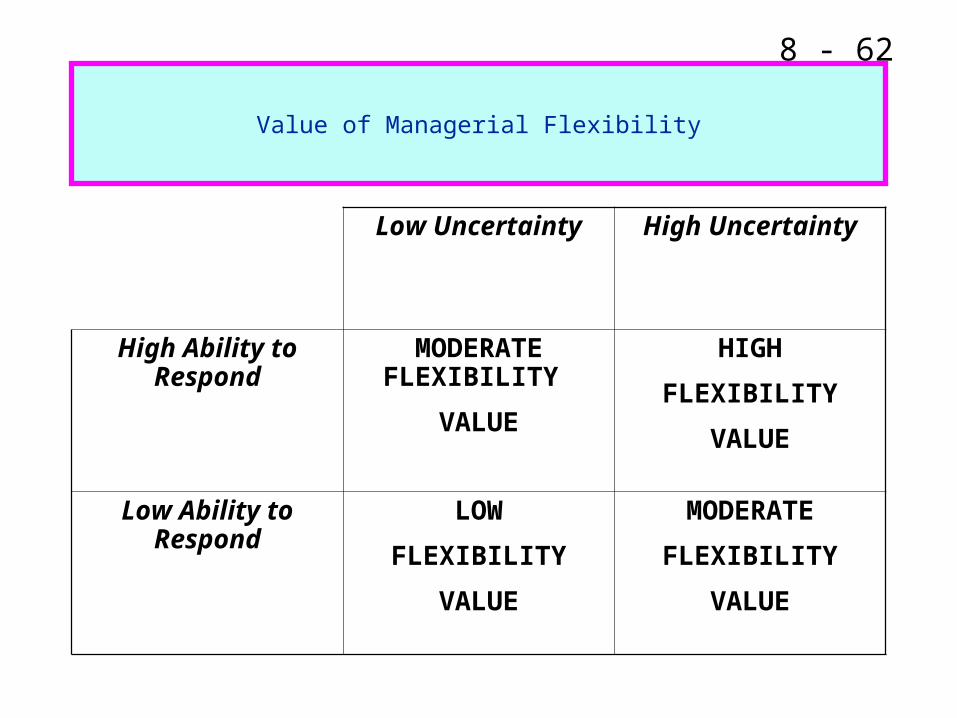
Value of Managerial Flexibility
Low Uncertainty High Uncertainty
High Ability to Respond
MODERATE FLEXIBILITY
VALUE
HIGH
FLEXIBILITY
VALUE
Low Ability to Respond
LOW
FLEXIBILITY
VALUE
MODERATE
FLEXIBILITY
VALUE
8 - 63
Decision Trees
Decision Tree Analysis is useful for applying binomial pricing methods to (real) options
Decision trees are used to analyze projects that involve sequential decisions
If the decision made today affects the decision that we are able to make tomorrow, then we should analyze tomorrow’s decision before we act today
8 - 64
Decision Trees
Example: Suppose that Delta Airlines is considering offering shuttle service between Champaign and Cincinnati for two years
Future demand for this service is uncertain and the company must make a decision today of what type of plane to buy
Suppose that there is a 60% chance that demand for this service will be high and 40% chance that it will be low after the service is initiated
If demand is high, there is a 75% chance that subsequent demand will also be high
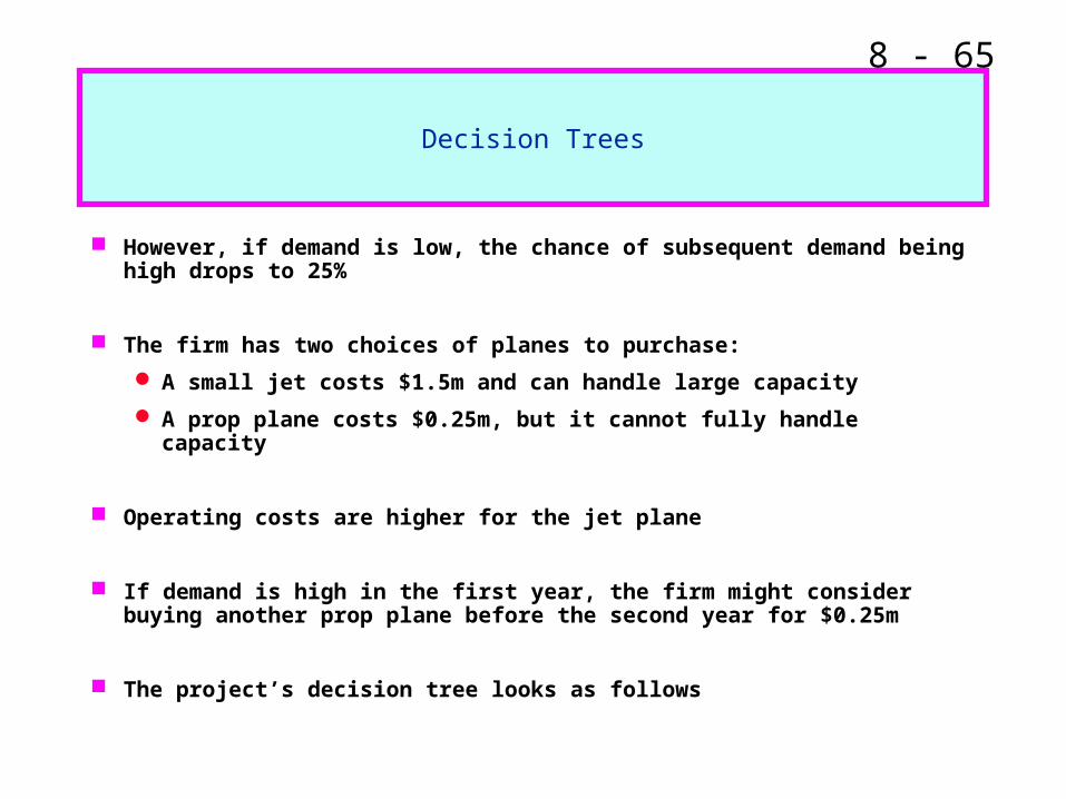
8 - 65
Decision Trees
However, if demand is low, the chance of subsequent demand being high drops to 25%
The firm has two choices of planes to purchase:
A small jet costs $1.5m and can handle large capacity
A prop plane costs $0.25m, but it cannot fully handle capacity
Operating costs are higher for the jet plane
If demand is high in the first year, the firm might consider buying another prop plane before the second year for $0.25m
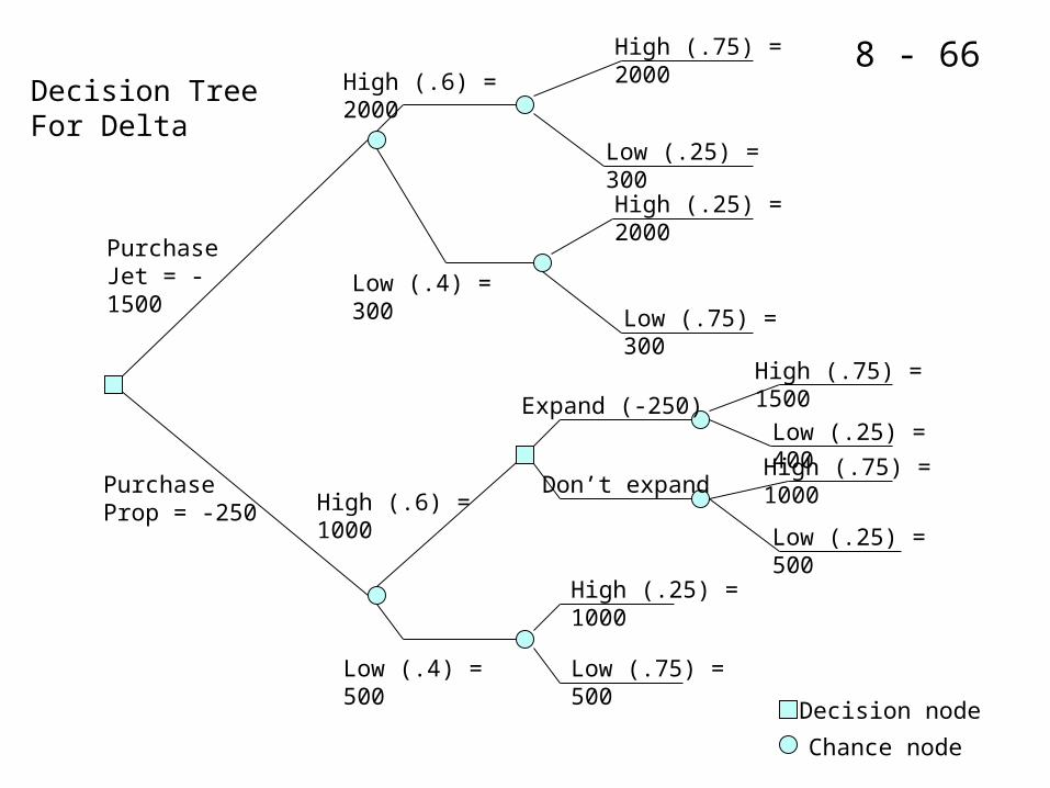
The project’s decision tree looks as follows
8 - 66
PurchaseJet = -1500
PurchaseProp = -250
Low (.4) = 300
High (.6) = 1000
High (.6) = 2000
Low (.4) = 500
High (.75) = 2000
High (.25) = 2000
High (.75) = 1500
High (.75) = 1000
High (.25) = 1000
Low (.25) = 300
Low (.75) = 300
Low (.25) = 400
Low (.25) = 500
Low (.75) = 500
Decision node
Chance node
Decision TreeFor Delta
Expand (-250)
Don’t expand