7 Magnetosphere

Michael Schulz

Earth’s magnetosphere is a fascinating repository ofcold plasma, hot plasma, and energetic charged par-ticles, all acting under the kinematical and dynamicalinfluence of electric andmagnetic fields, as well as un-der the influence of waves and instabilities, which theplasmas themselves control in turn. This chapter con-stitutes a largely theoretical overview of Earth’s mag-netosphere and the physical processes that govern it.

Contents

7.1 Introduction . . . . . . . . . . . . . . . . . . . . . . . . . . . . . . . . . . . 158

7.2 Magnetic Configuration . . . . . . . . . . . . . . . . . . . . . . . . . 159

7.3 Magnetospheric Electric Fields . . . . . . . . . . . . . . . . . . . 166

7.4 Magnetospheric Charged Particles . . . . . . . . . . . . . . . . 175

7.5 Summary . . . . . . . . . . . . . . . . . . . . . . . . . . . . . . . . . . . . . . 188

References . . . . . . . . . . . . . . . . . . . . . . . . . . . . . . . . . . . . . . . . . . . . . . 189

Michael Schulz, Magnetosphere.In: Y. Kamide/A. Chian, Handbook of the Solar-Terrestrial Environment. pp. – ()DOI: ./_ © Springer-Verlag Berlin Heidelberg

M. Schulz

7.1 Introduction

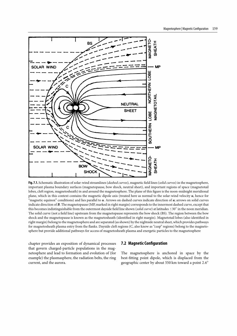
The magnetosphere (see Fig. 7.1) occupies a region ofspace within which the geomagnetic field is (in first ap-proximation) confined by the solar wind. It is boundedby a thin current layer called the magnetopause, whichis shaped somewhat like a windsock, and precededupstream by a hyperboloidal bow shock throughwhich the solar wind makes a transition from super-magnetosonic to sub-magnetosonic flow velocity. A gap� –RE (Earth radii, RE = . km by convention)separates the bow shock from the magnetopause alongthe Earth-Sun line because the magnetopause itselfpresents a blunt obstacle to the flowing solar wind.The size and shape of the magnetosphere are largelydetermined by pressure balance between the shockedsolar wind and the compressed geomagnetic field. Thenose of the magnetosphere is located (under nominalsolar-wind conditions) about RE upstream from thebest-fitting point dipole.

Orientation of the magnetosphere is controlled bythe direction of the solar wind, which is a highly ionizedplasma that flows outward from the Sun at velocitiesu � – km�s, with a mean value �u� � km�sat low (near-ecliptic) latitudes in the heliosphere.The solar-wind plasma is mostly hydrogenic (�%by number density) but also includes some helium,oxygen, and other ions in various charge states. Thetotal electron density Ne at r = AU (� r�) in theheliosphere varies considerably about its mean value�Ne� � cm−. (For reference: AU � . Gm, astro-nomical unit; r� � Mm, solar radius.) The radialcomponent of solar-wind velocity tends to increasewith heliospheric latitude (measured relative to theheliospheric current sheet) and thus shows both 27-dayand semi-annual variations at Earth. (The heliosphericcurrent sheet makes 14.5 rotations per year relativeto inertial space, but only 13.5 per year from Earth’sperspective.) Sudden variations in solar-wind speedand direction are associated with disturbances suchas coronal mass ejections and interplanetary shocks,which can directly impact the magnetosphere.

Magnetospheric dynamical processes are influencednot only by the solar wind itself, but also by the inter-planetary magnetic field (IMF), which emanates fromthe Sun and has its direction in the heliosphere largelycontrolled by the solar wind. The solar-wind speed u

at Earth’s orbit is � times the local Alfvén speed cA,which means that the solar wind has an energy density� times the local magnetic energy density B

�μ.(This chapter is written mostly in SI units, systèmeinternationale, also called mks, in which μ � π � −henry/meter denotes the permeability of free space.The energy density in cgs units would be written asB�π.)The strong inequality u cA in most of the heli-

osphere implies that plasma flow determines themagnetic-field configuration rather than the other wayaround. In order for a radially moving plasma elementto remain “forever” on the same field line as the Sunrotates, the field line itself must describe a large-scaleArchimedes spiral (Parker, 1963, pp. 138–139) in theheliosphere, being wrapped once around the Sun in theradial distance Δr (� . AU for u � km�s) that sucha plasma element travels during each solar rotation(� . days for global-scale magnetic features). Thismodel for the IMF is known as the Parker spiral, andthese particular parameters correspond to a local ratioBφ�Br � .π between the azimuthal and radialcomponents of BIMF at Earth’s orbit (hence to an angle� � between BIMF and the radial direction).

The angle between BIMF and u implies the pres-ence of an electric field E = −u � BIMF upstreamfrom the bow shock. Both the solar-wind plasma andthe IMF change direction and undergo compressionupon crossing the bow shock and thus entering themagnetosheath. The interplanetary electric field mapsinto the magnetosheath as well. Through a processcalled magnetic reconnection, particles and fields (bothelectric and magnetic) from the magnetosheath canpenetrate through the magnetopause and thereby enterthe magnetosphere. Reconnection at the magnetopauseis favored in regions where the magnetosheath B fieldmakes an angle � with the magnetospheric B field,and especially so at places where the magnetosheath Bfield is anti-parallel to the magnetospheric B field. Suchpenetration is of major importance for magnetosphericdynamics.

The present chapter offers a largely theoreticaloverview of magnetospheric structure and dynamics.It provides examples of modeling techniques thataim for realistic descriptions of the magnetosphericconfiguration, as well as modeling techniques thatlend themselves to analytical calculations. Finally, this

Magnetosphere | Magnetic Configuration

Fig. 7.1.Schematic illustration of solar-wind streamlines (dashed curves), magnetic field lines (solid curves) in themagnetosphere,important plasma boundary surfaces (magnetopause, bow shock, neutral sheet), and important regions of space (magnetotaillobes, cleft region, magnetosheath) in and around the magnetosphere. The plane of this figure is the noon-midnight meridionalplane, which in this context contains the magnetic dipole axis (treated here as normal to the solar-wind velocity u, hence for“magnetic equinox” conditions) and lies parallel to u. Arrows on dashed curves indicate direction of u; arrows on solid curvesindicate direction ofB. Themagnetopause (MP,marked in rightmargin) corresponds to the innermost dashed curve, except thatthis becomes indistinguishable from the outermost dayside field line shown (solid curve) at latitudes <� � in the noonmeridian.The solid curve (not a field line) upstream from the magnetopause represents the bow shock (BS). The region between the bowshock and the magnetopause is known as the magnetosheath (identified in right margin). Magnetotail lobes (also identified inrightmargin) belong to themagnetosphere and are separated (as shown) by the nightside neutral sheet, whichprovides pathwaysfor magnetosheath plasma entry from the flanks. Dayside cleft regions (C, also know as “cusp” regions) belong to the magneto-sphere but provide additional pathways for access of magnetosheath plasma and energetic particles to the magnetosphere

chapter provides an exposition of dynamical processesthat govern charged-particle populations in the mag-netosphere and lead to formation and evolution of (forexample) the plasmasphere, the radiation belts, the ringcurrent, and the aurora.

7.2 Magnetic Configuration

The magnetosphere is anchored in space by thebest-fitting point dipole, which is displaced from thegeographic center by about km toward a point .�

M. Schulz

south of Iwo Jima. The geomagnetic dipole moment μE(� .G-R

E at present) is tilted .� relative to theEarth’s rotation axis; it lies parallel to the plane definedby geographic meridians .� E and .�W. Becauseof the offset, however, the geomagnetic dipole axispierces the Earth’s surface about � and �, respectively,from the northern and southern geographic poles.The corresponding magnetic geometry is illustrated inFig. 7.2.

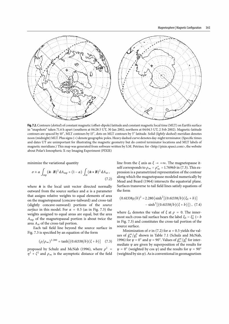
It is customary in magnetospheric physics to meas-uremagnetic colatitude θ from the offset-dipole axis andan azimuthal coordinate φ (called magnetic local time,MLT) from the plane that contains the offset-dipole axisand lies parallel to the Sun-Earth line.Magnetic-latitudecontours in Fig. 7.2 are separated by �, and MLT con-tours are separated by �(= h).

Themagnetosphere itself is oriented by the apparentdirection of the solar wind in Earth’s frame of reference.This means that account must be taken of Earth’s orbitalvelocity (� km�s) around the Sun, as well as the ra-dial and any non-radial component of solar-windvelocity in the heliosphere, in order to account well formagnetosphere’s orientation in space. The geomagnetictail’s orientation is thus essentially (but not perfectly)anti-sunward. The effect of Earth’s orbital velocity onmagnetospheric orientation is known as aberration.There is no particular name for the magnetosphericconsequences of an azimuthal component of solar-windvelocity in the heliosphere. Earth’s orbital velocity(� km�s) leads to an aberration (�.� for solar-windvelocity u � km�s) in the apparent mean directionof the solar wind relative to the Sun-Earth line, but thiseffect is partially offset by the azimuthal component(� km�s) of the solar-wind velocity at r = AU in theheliosphere.

An angle of major significance for magnetosphericgeometry is the angle ψ between the dipole moment μEand the solar-wind velocity u in Earth’s reference frame.This angle varies systematically (with season of year andhour of day) between .� and .�, as well as spo-radically in response to variations in solar-wind veloc-ity. The extrema in ψ correspond to “magnetic-solstice”conditions, whereas ψ = � corresponds to “magneticequinox.” The plane that contains the offset-dipole axisand lies parallel to the aberrated solar-wind velocity thusbisects the magnetosphere between AM and PM halvesthat are (in first approximation) mirror images of eachother.

Figure 7.3 (Schulz and McNab, 1996) illustrates anidealized magnetosphere at magnetic equinox (upperpanels) and near magnetic solstice (lower panels), re-spectively. The coordinate ξ is measured from a planethat contains the “point dipole” and lies transverse to theaberrated solar-wind velocity (i.e., as realized upstreamfrom the bow shock). The coordinate η in Fig. 7.3 ismeasured from the plane (see above) that contains theoffset-dipole axis and lies parallel to the aberrated solar-wind velocity. The coordinate ζ is measured from theplane that contains the “point dipole” and lies perpen-dicular to these other two planes.

The coordinates in Fig. 7.3 thus differ in subtle waysfrom the (X, Y , Z) coordinates of the standard GSM(geocentric solar magnetospheric) system in whichdata from spacecraft are usually presented. As the nameimplies, GSM coordinates are Earth-centered ratherthan dipole-centered. Moreover, XGSM is measuredtoward the Sun from a plane perpendicular to theEarth-Sun line, and YGSM is measured from a plane thatcontains the geocenter and lies parallel to the magneticdipole axis. Finally, ZGSM is measured from a plane thatcontains the geocenter and lies perpendicular to theseother two planes. The differences between these tworight-handed systems, (ξ, η, ζ) and GSM, are unimpor-tant for general orientation, except that ξ correspondsroughly to −XGSM and η corresponds roughly to −YGSM.However, some care must be taken when makingdetailed comparisons between theoretical models andin situ data, to be sure that both are expressed in thesame coordinate system for this purpose.

The model B field illustrated in Fig. 7.3 is derivedfrom a scalar potential expanded in spherical harmon-ics:

B(r, θ , φ) =

− g∇[(a�r) cos θ]

− (a�b)∇N

�

n=

n

�

m=gmn (r�b)

nPmn (θ) cosmφ , (7.1)

where a = RE and b is the distance from the pointdipole to the “nose” of themagnetopause. The colatitudeθ in (7.1) ismeasured from themagnetic dipole axis, andthe MLT coordinate φ is measured from the plane thatcontains the dipole axis and lies parallel to the aberratedsolar-wind velocity u. The expansion coefficients � gmn in (7.1) are chosen (Schulz and McNab, 1996) so as to

Magnetosphere | Magnetic Configuration

Fig. 7.2.Contours (dotted) of constantmagnetic (offset-dipole) latitude and constantmagnetic local time (MLT) onEarth’s surfacein “snapshots” taken . h apart (southern at 04:28.5 UT, 30 Jan 2002; northern at 04:04.5 UT, 2 Feb 2002). Magnetic-latitudecontours are spaced by �, MLT contours by �, dots on MLT contours by � latitude. Solid (lightly dashed) meridian denotesnoon (midnight)MLT. Plus signs (+) denote geographic poles.Heavy dashed curve denotes day-night terminator. (Specific timesand dates UT are unimportant for illustrating the magnetic geometry but do control terminator locations and MLT labels ofmagnetic meridians.) This map was generated from software written by S.M. Petrinec for <http://pixie.spasci.com>, the websiteabout Polar’s Ionospheric X-ray Imaging Experiment (PIXIE)

minimize the variational quantity

σ � α�

mp(n ċ B) dAmp + ( − α)

�

xt(n � B) dAxt ,

(7.2)

where n is the local unit vector directed normallyoutward from the source surface and α is a parameterthat assigns relative weights to equal elements of areaon the magnetopausal (concave-tailward) and cross-tail(slightly concave-sunward) portions of the sourcesurface in this model. For α = . (as in Fig. 7.3) theweights assigned to equal areas are equal, but the areaAmp of the magnetopausal portion is about twice thearea Axt of the cross-tail portion.

Each tail field line beyond the source surface inFig. 7.3 is specified by an equation of the form

(ρ�ρ�). = tanh[(.�b)(ξ + b)] (7.3)

proposed by Schulz and McNab (1996), where ρ =

η + ζ and ρ� is the asymptotic distance of the field

line from the ξ axis as ξ � +�. The magnetopause it-self corresponds to ρ� = ρ�

�= .b in (7.3). This ex-

pression is a parametrized representation of the contouralong which the magnetopause modeled numerically byMead and Beard (1964) intersects the equatorial plane.Surfaces transverse to tail field lines satisfy equations ofthe form

(.ρ�b) = .�sinh[(.�b)(ξ + b)]

− sinh[(.�b)(ξ + b)] , (7.4)

where ξ denotes the value of ξ at ρ = . The inner-most such cross-tail surface bears the label ξ = ξ� (= bin Fig. 7.3) and constitutes the cross-tail portion of thesource surface.

Minimization of σ in (7.2) for α = . yields the val-ues of gmn �g shown in Table 7.1 (Schulz and McNab,1996) for ψ = � and ψ = �. Values of gmn �g for inter-mediate ψ are given by superposition of the results forψ = � (weighted by cos ψ) and the results for ψ = �(weighted by sinψ). As is conventional in geomagnetism

M. Schulz

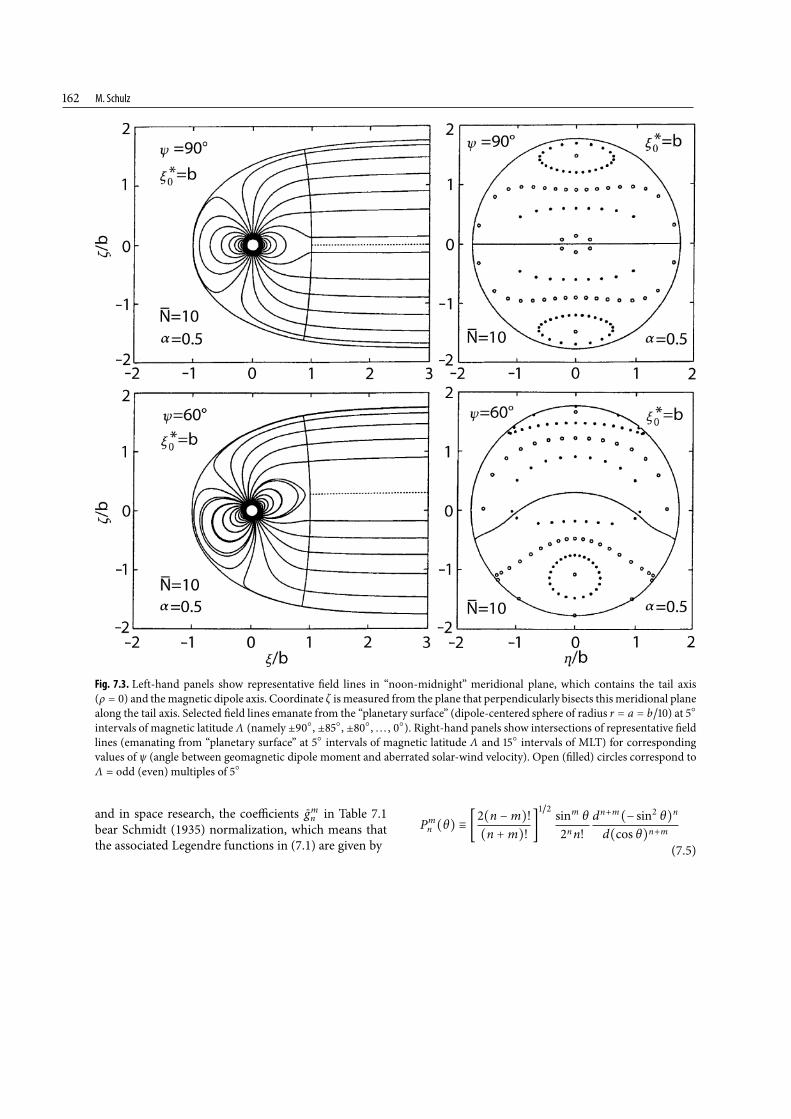
Fig. 7.3. Left-hand panels show representative field lines in “noon-midnight” meridional plane, which contains the tail axis(ρ = ) and the magnetic dipole axis. Coordinate ζ is measured from the plane that perpendicularly bisects this meridional planealong the tail axis. Selected field lines emanate from the “planetary surface” (dipole-centered sphere of radius r = a = b�) at �

intervals of magnetic latitude Λ (namely ��, ��, �� , . . . , �). Right-hand panels show intersections of representative fieldlines (emanating from “planetary surface” at � intervals of magnetic latitude Λ and � intervals of MLT) for correspondingvalues of ψ (angle between geomagnetic dipole moment and aberrated solar-wind velocity). Open (filled) circles correspond toΛ = odd (even) multiples of �

and in space research, the coefficients gmn in Table 7.1bear Schmidt (1935) normalization, which means thatthe associated Legendre functions in (7.1) are given by

Pmn (θ) � �

(n −m)!(n +m)!

�

� sinm θnn!

dn+m(− sin θ)n

d(cos θ)n+m(7.5)

Magnetosphere | Magnetic Configuration

form but by (�)� of this form = . Usually omit-ted for all values of m in mathematics books and fromlibrary routines for computers, the square-bracketedfactor in (7.5) makes the contribution of degree n tothe mean value of B, produced over a sphere of radiusr < min(b, ξ� ) by magnetospheric currents, propor-tional to the unweighted sum (over m) of the squaresof the expansion coefficients gmn . In other words, therelative influence of various terms (with different valuesof m) in the expansion for B is accurately reflected bythe relative magnitudes of their Schmidt-normalizedexpansion coefficients.

The B field illustrated in Fig. 7.3 and the considera-tions behind it represent only one of many approachesto magnetospheric modeling. A different school ofthought, exemplified by the work of Tsyganenko (1995),calls for the magnetospheric B field to be representedby globally fitting empirical data on B to a series ofanalytical functions corresponding to various magneto-spheric current systems. Representative results shown

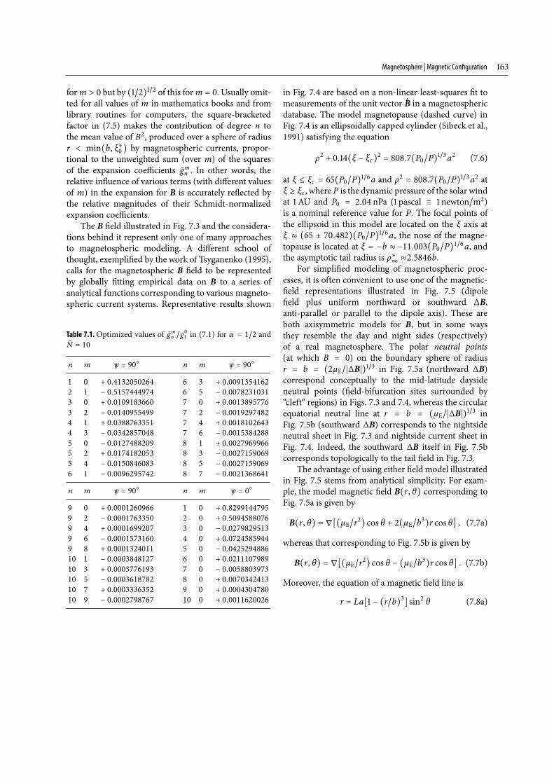
Table 7.1.Optimized values of gmn �g01 in (7.1) for α = 1�2 andN = 10

n m ψ = 90� n m ψ = 90�

1 0 + 0.4132050264 6 3 + 0.00913541622 1 − 0.5157444974 6 5 − 0.00782310313 0 + 0.0109183660 7 0 + 0.00138957763 2 − 0.0140955499 7 2 − 0.00192974824 1 + 0.0388763351 7 4 + 0.00181026434 3 − 0.0342857048 7 6 − 0.00153842885 0 − 0.0127488209 8 1 + 0.00279699665 2 + 0.0174182053 8 3 − 0.00271590695 4 − 0.0150846083 8 5 − 0.00271590696 1 − 0.0096295742 8 7 − 0.0021368641

n m ψ = 90� n m ψ = 0�

9 0 + 0.0001260966 1 0 + 0.82991447959 2 − 0.0001763350 2 0 + 0.50945880769 4 + 0.0001699207 3 0 − 0.02798295139 6 − 0.0001573160 4 0 + 0.07245859449 8 + 0.0001324011 5 0 − 0.042529488610 1 − 0.0003848127 6 0 + 0.021110798910 3 + 0.0003776193 7 0 − 0.005880397310 5 − 0.0003618782 8 0 + 0.007034241310 7 + 0.0003336352 9 0 + 0.000430478010 9 − 0.0002798767 10 0 + 0.0011620026

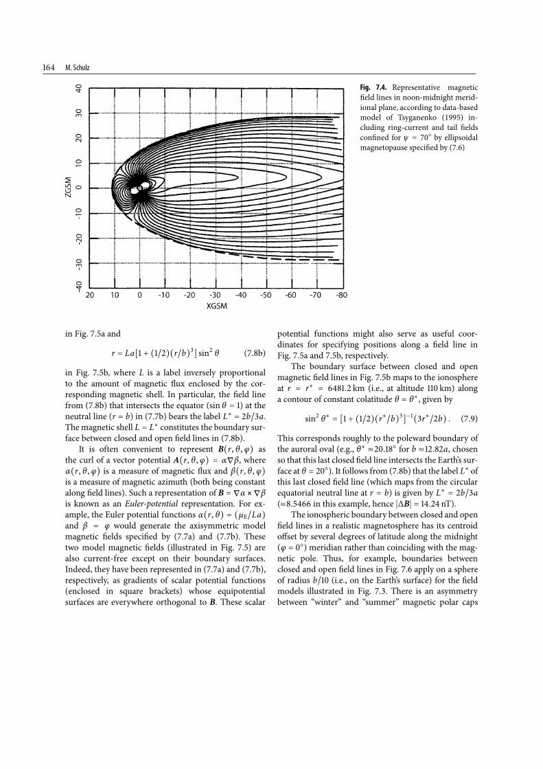
in Fig. 7.4 are based on a non-linear least-squares fit tomeasurements of the unit vector B in a magnetosphericdatabase. The model magnetopause (dashed curve) inFig. 7.4 is an ellipsoidally capped cylinder (Sibeck et al.,1991) satisfying the equation

ρ + .(ξ − ξc) = .(P�P)�a (7.6)

at ξ � ξc = (P�P)�a and ρ = .(P�P)�a atξ � ξc , where P is the dynamic pressure of the solar windat AU and P = . nPa ( pascal � newton�m)is a nominal reference value for P. The focal points ofthe ellipsoid in this model are located on the ξ axis atξ � ( � .)(P�P)�a, the nose of the magne-topause is located at ξ = −b � −11.003(P0�P)1�6a, andthe asymptotic tail radius is ρ�

��.b.

For simplified modeling of magnetospheric proc-esses, it is often convenient to use one of the magnetic-field representations illustrated in Fig. 7.5 (dipolefield plus uniform northward or southward ΔB,anti-parallel or parallel to the dipole axis). These areboth axisymmetric models for B, but in some waysthey resemble the day and night sides (respectively)of a real magnetosphere. The polar neutral points(at which B = ) on the boundary sphere of radiusr = b = (μE��ΔB�)� in Fig. 7.5a (northward ΔB)correspond conceptually to the mid-latitude daysideneutral points (field-bifurcation sites surrounded by“cleft” regions) in Figs. 7.3 and 7.4, whereas the circularequatorial neutral line at r = b = (μE��ΔB�)� inFig. 7.5b (southward ΔB) corresponds to the nightsideneutral sheet in Fig. 7.3 and nightside current sheet inFig. 7.4. Indeed, the southward ΔB itself in Fig. 7.5bcorresponds topologically to the tail field in Fig. 7.3.

The advantage of using either field model illustratedin Fig. 7.5 stems from analytical simplicity. For exam-ple, the model magnetic field B(r, θ) corresponding toFig. 7.5a is given by

B(r, θ) = ∇[(μE�r) cos θ + (μE�b)r cos θ] , (7.7a)

whereas that corresponding to Fig. 7.5b is given by

B(r, θ) = ∇[(μE�r) cos θ − (μE�b)r cos θ] . (7.7b)

Moreover, the equation of a magnetic field line is

r = La[ − (r�b)] sin θ (7.8a)

M. Schulz

Fig. 7.4. Representative magneticfield lines in noon-midnight merid-ional plane, according to data-basedmodel of Tsyganenko (1995) in-cluding ring-current and tail fieldsconfined for ψ = � by ellipsoidalmagnetopause specified by (7.6)

in Fig. 7.5a and

r = La[ + (�)(r�b)] sin θ (7.8b)

in Fig. 7.5b, where L is a label inversely proportionalto the amount of magnetic flux enclosed by the cor-responding magnetic shell. In particular, the field linefrom (7.8b) that intersects the equator (sin θ = ) at theneutral line (r = b) in (7.7b) bears the label L� = b�a.Themagnetic shell L = L� constitutes the boundary sur-face between closed and open field lines in (7.8b).

It is often convenient to represent B(r, θ , φ) asthe curl of a vector potential A(r, θ , φ) = α∇β, whereα(r, θ , φ) is a measure of magnetic flux and β(r, θ , φ)is a measure of magnetic azimuth (both being constantalong field lines). Such a representation of B = ∇α �∇βis known as an Euler-potential representation. For ex-ample, the Euler potential functions α(r, θ) = (μE�La)and β = φ would generate the axisymmetric modelmagnetic fields specified by (7.7a) and (7.7b). Thesetwo model magnetic fields (illustrated in Fig. 7.5) arealso current-free except on their boundary surfaces.Indeed, they have been represented in (7.7a) and (7.7b),respectively, as gradients of scalar potential functions(enclosed in square brackets) whose equipotentialsurfaces are everywhere orthogonal to B. These scalar

potential functions might also serve as useful coor-dinates for specifying positions along a field line inFig. 7.5a and 7.5b, respectively.

The boundary surface between closed and openmagnetic field lines in Fig. 7.5b maps to the ionosphereat r = r� = . km (i.e., at altitude km) alonga contour of constant colatitude θ = θ�, given by

sin θ� = [ + (�)(r��b)]−(r��b) . (7.9)

This corresponds roughly to the poleward boundary ofthe auroral oval (e.g., θ� �.� for b � .a, chosenso that this last closed field line intersects the Earth’s sur-face at θ = �). It follows from (7.8b) that the label L� ofthis last closed field line (which maps from the circularequatorial neutral line at r = b) is given by L� = b�a(�. in this example, hence �ΔB� = . nT).

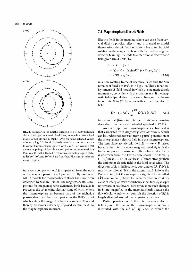
The ionospheric boundary between closed and openfield lines in a realistic magnetosphere has its centroidoffset by several degrees of latitude along the midnight(φ = �) meridian rather than coinciding with the mag-netic pole. Thus, for example, boundaries betweenclosed and open field lines in Fig. 7.6 apply on a sphereof radius b� (i.e., on the Earth’s surface) for the fieldmodels illustrated in Fig. 7.3. There is an asymmetrybetween “winter” and “summer” magnetic polar caps

Magnetosphere | Magnetic Configuration

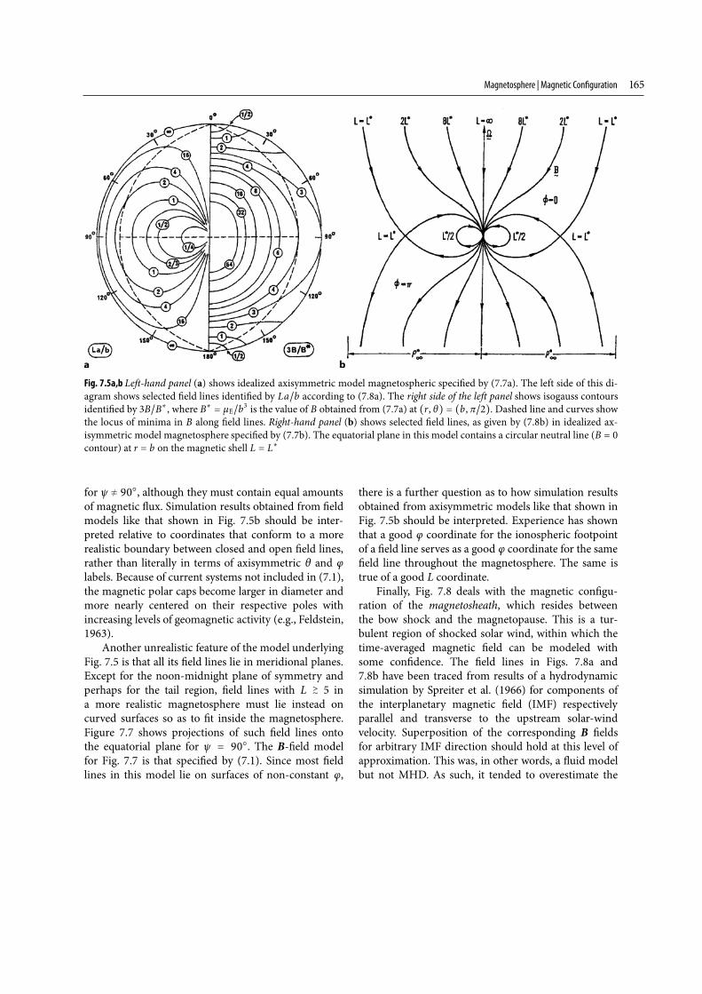
Fig. 7.5a,b Left-hand panel (a) shows idealized axisymmetric model magnetospheric specified by (7.7a). The left side of this di-agram shows selected field lines identified by La�b according to (7.8a). The right side of the left panel shows isogauss contoursidentified by B�B�, where B� = μE�b is the value of B obtained from (7.7a) at (r, θ) = (b, π�). Dashed line and curves showthe locus of minima in B along field lines. Right-hand panel (b) shows selected field lines, as given by (7.8b) in idealized ax-isymmetric model magnetosphere specified by (7.7b). The equatorial plane in this model contains a circular neutral line (B = contour) at r = b on the magnetic shell L = L�

for ψ � �, although they must contain equal amountsof magnetic flux. Simulation results obtained from fieldmodels like that shown in Fig. 7.5b should be inter-preted relative to coordinates that conform to a morerealistic boundary between closed and open field lines,rather than literally in terms of axisymmetric θ and φlabels. Because of current systems not included in (7.1),the magnetic polar caps become larger in diameter andmore nearly centered on their respective poles withincreasing levels of geomagnetic activity (e.g., Feldstein,1963).

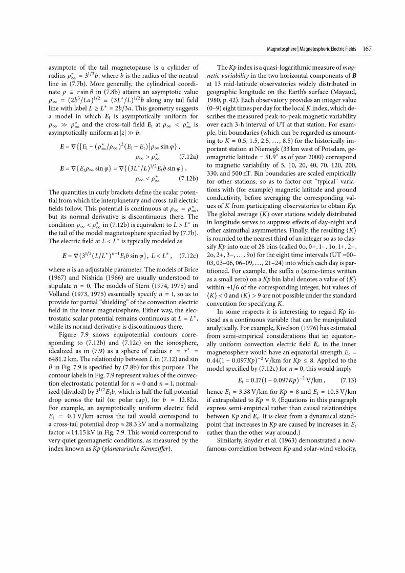
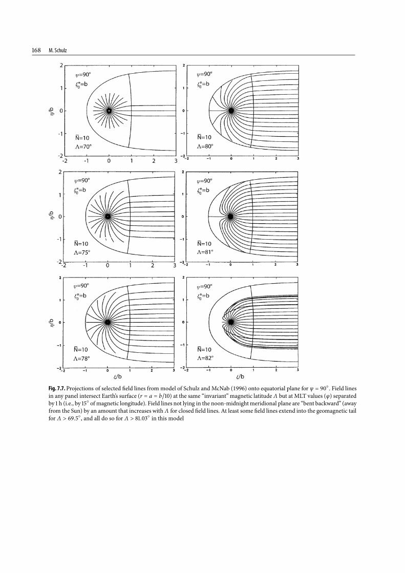
Another unrealistic feature of the model underlyingFig. 7.5 is that all its field lines lie in meridional planes.Except for the noon-midnight plane of symmetry andperhaps for the tail region, field lines with L �

� ina more realistic magnetosphere must lie instead oncurved surfaces so as to fit inside the magnetosphere.Figure 7.7 shows projections of such field lines ontothe equatorial plane for ψ = �. The B-field modelfor Fig. 7.7 is that specified by (7.1). Since most fieldlines in this model lie on surfaces of non-constant φ,

there is a further question as to how simulation resultsobtained from axisymmetric models like that shown inFig. 7.5b should be interpreted. Experience has shownthat a good φ coordinate for the ionospheric footpointof a field line serves as a good φ coordinate for the samefield line throughout the magnetosphere. The same istrue of a good L coordinate.

Finally, Fig. 7.8 deals with the magnetic configu-ration of the magnetosheath, which resides betweenthe bow shock and the magnetopause. This is a tur-bulent region of shocked solar wind, within which thetime-averaged magnetic field can be modeled withsome confidence. The field lines in Figs. 7.8a and7.8b have been traced from results of a hydrodynamicsimulation by Spreiter et al. (1966) for components ofthe interplanetary magnetic field (IMF) respectivelyparallel and transverse to the upstream solar-windvelocity. Superposition of the corresponding B fieldsfor arbitrary IMF direction should hold at this level ofapproximation. This was, in other words, a fluid modelbut not MHD. As such, it tended to overestimate the

M. Schulz

Fig. 7.6.Boundaries (on Earth’s surface, r = a = b�) betweenclosed and open magnetic field lines, as obtained from fieldmodel of Schulz and McNab (1996) for same selected valuesof ψ as in Fig. 7.3. Solid (dashed) boundary contours pertainto winter (summer) hemisphere for ψ = �. Sun symbols (�)denote mappings of dayside neutral points on noon meridian(Sun is at the left.). Dotted circles correspond tomagnetic lati-tudes �, �, and � onEarth’s surface. Plus signs (+) denotemagnetic poles

transverse component of B just upstream from the noseof the magnetopause. Development of fully nonlinearMHD models for magnetosheath flows has since beendescribed by Stahara (2002). The magnetosheath is im-portant for magnetospheric dynamics, both because itprocesses the solar-wind plasma (some of which entersthe magnetosphere to become part of the nightsideplasma sheet) and because it processes the IMF (part ofwhich enters the magnetosphere via reconnection andthereby transmits externally imposed electric fields tothe magnetospheric interior).

7.3 Magnetospheric Electric Fields

Electric fields in the magnetosphere can arise from sev-eral distinct physical effects, and it is usual to modelthese various electric fields separately. For example, rigidrotation of the magnetosphere with the Earth at angularvelocity Ω in Fig. 7.5 leads to a meridional electrostaticfield given (in SI units) by

E = −(Ω � r) � B

= (Ω � r) � [(r sin θ)−φ � ∇(μE�La)]= −Ω∇(μE�La) . (7.10)

in a non-rotating frame of reference (such that the Sunremains at fixed φ = �, as in Fig. 7.7). This is for an ax-isymmetric B-fieldmodel, in which the magnetic dipolemoment μE coincides with the rotation axis. If the mag-netic field slips relative to the ionosphere, so that the ro-tation rate Ω in (7.10) varies with L, then the electricfield

E = −(μE�a)∇��L

Ω(L′)d(�L′) (7.11)

in an inertial (fixed-Sun) frame of reference remainsderivable from the scalar potential specified in (7.11).

Another important magnetospheric electric field isthat associated with magnetospheric convection, whichcan be understood to result from a partial penetration ofthe interplanetary electric field into the magnetosphere.The interplanetary electric field Ei = −u � Bi arisesbecause the interplanetary magnetic field Bi typicallyhas a component transverse to the solar-wind velocityu upstream from the Earth’s bow shock. The local Ei(� V�km at R = AU) is at least 10 times stronger thanthe ambipolar electric field in the local solar wind. Thedirection of Ei in heliospheric coordinates (R, T , N) ismostly meridional (N) to the extent that Bi follows theParker spiral, but Ei can acquire a significant azimuthal(T) component (relative to the Sun’s rotation axis) be-cause of interplanetary disturbances that turn Bi sharplynorthward or southward. Moreover, some such changesin Bi are magnified in the magnetosheath because theflow of solar wind (which controls the direction of Bi) islargely diverted around the magnetopause there.

Partial penetration of the interplanetary electricfield Ei into the tail of the magnetosphere is nicelyillustrated with the aid of Fig. 7.5b, in which the

Magnetosphere | Magnetospheric Electric Fields

asymptote of the tail magnetopause is a cylinder ofradius ρ�

�= �b, where b is the radius of the neutral

line in (7.7b). More generally, the cylindrical coordi-nate ρ � r sin θ in (7.8b) attains an asymptotic valueρ� = (b�La)� � (L��L)�b along any tail fieldline with label L � L� � b�a. This geometry suggestsa model in which Ei is asymptotically uniform forρ� ρ�

�and the cross-tail field Et at ρ� < ρ�

�is

asymptotically uniform at �z� b:

E = ∇�[Ei − (ρ���ρ�)(Ei − Et)]ρ� sin φ ,

ρ� ρ��

(7.12a)

E = ∇�Etρ� sin φ = ∇�(L��L)�Etb sin φ ,ρ� < ρ�

�(7.12b)

The quantities in curly brackets define the scalar poten-tial fromwhich the interplanetary and cross-tail electricfields follow. This potential is continuous at ρ� = ρ�

�,

but its normal derivative is discontinuous there. Thecondition ρ� < ρ�

�in (7.12b) is equivalent to L > L� in

the tail of the model magnetosphere specified by (7.7b).The electric field at L < L� is typically modeled as

E = ∇��(L�L�)n+Etb sin φ , L < L� , (7.12c)

where n is an adjustable parameter. The models of Brice(1967) and Nishida (1966) are usually understood tostipulate n = . The models of Stern (1974, 1975) andVolland (1973, 1975) essentially specify n = , so as toprovide for partial “shielding” of the convection electricfield in the inner magnetosphere. Either way, the elec-trostatic scalar potential remains continuous at L = L�,while its normal derivative is discontinuous there.

Figure 7.9 shows equipotential contours corre-sponding to (7.12b) and (7.12c) on the ionosphere,idealized as in (7.9) as a sphere of radius r = r� =

6481.2 km. The relationship between L in (7.12) and sinθ in Fig. 7.9 is specified by (7.8b) for this purpose. Thecontour labels in Fig. 7.9 represent values of the convec-tion electrostatic potential for n = and n = , normal-ized (divided) by �Etb, which is half the full potentialdrop across the tail (or polar cap), for b = .a.For example, an asymptotically uniform electric fieldEt = 0.1 V�km across the tail would correspond toa cross-tail potential drop � . kV and a normalizingfactor � 14.15 kV in Fig. 7.9. This would correspond tovery quiet geomagnetic conditions, as measured by theindex known as Kp (planetarische Kennziffer).

TheKp index is a quasi-logarithmicmeasure ofmag-netic variability in the two horizontal components of Bat 13 mid-latitude observatories widely distributed ingeographic longitude on the Earth’s surface (Mayaud,1980, p. 42). Each observatory provides an integer value(0–9) eight times per day for the localK index, which de-scribes the measured peak-to-peak magnetic variabilityover each 3-h interval of UT at that station. For exam-ple, bin boundaries (which can be regarded as amount-ing to K = ., 1.5, 2.5, . . . , 8.5) for the historically im-portant station at Niemegk ( km west of Potsdam, ge-omagnetic latitude = .� as of year 2000) correspondto magnetic variability of 5, 10, 20, 40, 70, 120, 200,330, and nT. Bin boundaries are scaled empiricallyfor other stations, so as to factor-out “typical” varia-tions with (for example) magnetic latitude and groundconductivity, before averaging the corresponding val-ues of K from participating observatories to obtain Kp.The global average �K� over stations widely distributedin longitude serves to suppress effects of day-night andother azimuthal asymmetries. Finally, the resulting �K�is rounded to the nearest third of an integer so as to clas-sify Kp into one of 28 bins (called 0o, +, −, 1o, +, −,2o, +, −, . . . , 9o) for the eight time intervals (UT =00–03, 03–06, 06–09, . . . , 21–24) into which each day is par-titioned. For example, the suffix o (some-times writtenas a small zero) on a Kp bin label denotes a value of �K�within �� of the corresponding integer, but values of�K� < and �K� are not possible under the standardconvention for specifying K.

In some respects it is interesting to regard Kp in-stead as a continuous variable that can be manipulatedanalytically. For example, Kivelson (1976) has estimatedfrom semi-empirical considerations that an equatori-ally uniform convection electric field Ec in the innermagnetosphere would have an equatorial strength Ec =

.( − .Kp)− V�km for Kp � . Applied to themodel specified by (7.12c) for n = , this would imply

Et = .( − .Kp)− V�km , (7.13)

hence Et = .V�km for Kp = and Et = 10.5 V�kmif extrapolated to Kp = . (Equations in this paragraphexpress semi-empirical rather than causal relationshipsbetween Kp and Ec. It is clear from a dynamical stand-point that increases in Kp are caused by increases in Etrather than the other way around.)

Similarly, Snyder et al. (1963) demonstrated a now-famous correlation between Kp and solar-wind velocity,

M. Schulz

Fig. 7.7.Projections of selected field lines from model of Schulz and McNab (1996) onto equatorial plane for ψ = �. Field linesin any panel intersect Earth’s surface (r = a = b�) at the same “invariant” magnetic latitude Λ but at MLT values (φ) separatedby h (i.e., by � of magnetic longitude). Field lines not lying in the noon-midnightmeridional plane are “bent backward” (awayfrom the Sun) by an amount that increases with Λ for closed field lines. At least some field lines extend into the geomagnetic tailfor Λ � .�, and all do so for Λ � .� in this model

Magnetosphere | Magnetospheric Electric Fields

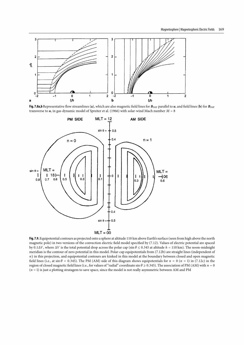
Fig. 7.8a,bRepresentative flow streamlines (a), which are alsomagnetic field lines for BIMF parallel to u, and field lines (b) for BIMF

transverse to u, in gas-dynamic model of Spreiter et al. (1966) with solar-windMach number M =

Fig. 7.9.Equipotential contours as projected onto a sphere at altitude 110 kmabove Earth’s surface (seen fromhigh above the northmagnetic pole) in two versions of the convection electric field model specified by (7.12). Values of electric potential are spacedby 0.1ΔV , where ΔV is the total potential drop across the polar cap (sin θ � . at altitude h = 110 km). The noon-midnightmeridian is the contour of zero potential in this model. Polar-cap equipotentials from (7.12b) are straight lines (independent ofn) in this projection, and equipotential contours are kinked in this model at the boundary between closed and open magneticfield lines (i.e., at sin θ = .). The PM (AM) side of this diagram shows equipotentials for n = (n = ) in (7.12c) in theregion of closed magnetic field lines (i.e., for values of “radial” coordinate sin θ � .). The association of PM (AM)with n = (n = ) is just a plotting stratagem to save space, since the model is not really asymmetric between AM and PM

M. Schulz

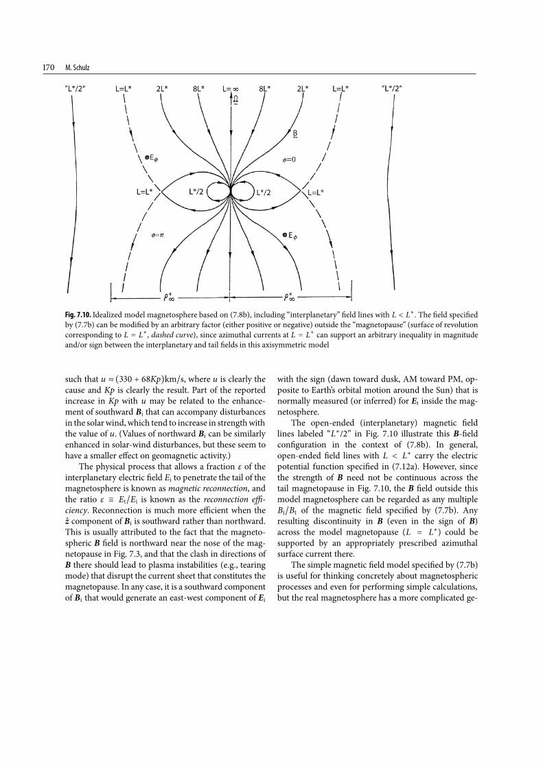
Fig. 7.10. Idealized model magnetosphere based on (7.8b), including “interplanetary” field lines with L < L�. The field specifiedby (7.7b) can be modified by an arbitrary factor (either positive or negative) outside the “magnetopause” (surface of revolutioncorresponding to L = L�, dashed curve), since azimuthal currents at L = L� can support an arbitrary inequality in magnitudeand/or sign between the interplanetary and tail fields in this axisymmetric model

such that u � ( + Kp)km�s, where u is clearly thecause and Kp is clearly the result. Part of the reportedincrease in Kp with u may be related to the enhance-ment of southward Bi that can accompany disturbancesin the solarwind,which tend to increase in strengthwiththe value of u. (Values of northward Bi can be similarlyenhanced in solar-wind disturbances, but these seem tohave a smaller effect on geomagnetic activity.)

The physical process that allows a fraction ε of theinterplanetary electric field Ei to penetrate the tail of themagnetosphere is known as magnetic reconnection, andthe ratio ε � Et�Ei is known as the reconnection effi-ciency. Reconnection is much more efficient when thez component of Bi is southward rather than northward.This is usually attributed to the fact that the magneto-spheric B field is northward near the nose of the mag-netopause in Fig. 7.3, and that the clash in directions ofB there should lead to plasma instabilities (e.g., tearingmode) that disrupt the current sheet that constitutes themagnetopause. In any case, it is a southward componentof Bi that would generate an east-west component of Ei

with the sign (dawn toward dusk, AM toward PM, op-posite to Earth’s orbital motion around the Sun) that isnormally measured (or inferred) for Et inside the mag-netosphere.

The open-ended (interplanetary) magnetic fieldlines labeled “L�/2” in Fig. 7.10 illustrate this B-fieldconfiguration in the context of (7.8b). In general,open-ended field lines with L < L� carry the electricpotential function specified in (7.12a). However, sincethe strength of B need not be continuous across thetail magnetopause in Fig. 7.10, the B field outside thismodel magnetosphere can be regarded as any multipleBi�Bt of the magnetic field specified by (7.7b). Anyresulting discontinuity in B (even in the sign of B)across the model magnetopause (L = L�) could besupported by an appropriately prescribed azimuthalsurface current there.

The simple magnetic field model specified by (7.7b)is useful for thinking concretely about magnetosphericprocesses and even for performing simple calculations,but the real magnetosphere has a more complicated ge-

Magnetosphere | Magnetospheric Electric Fields

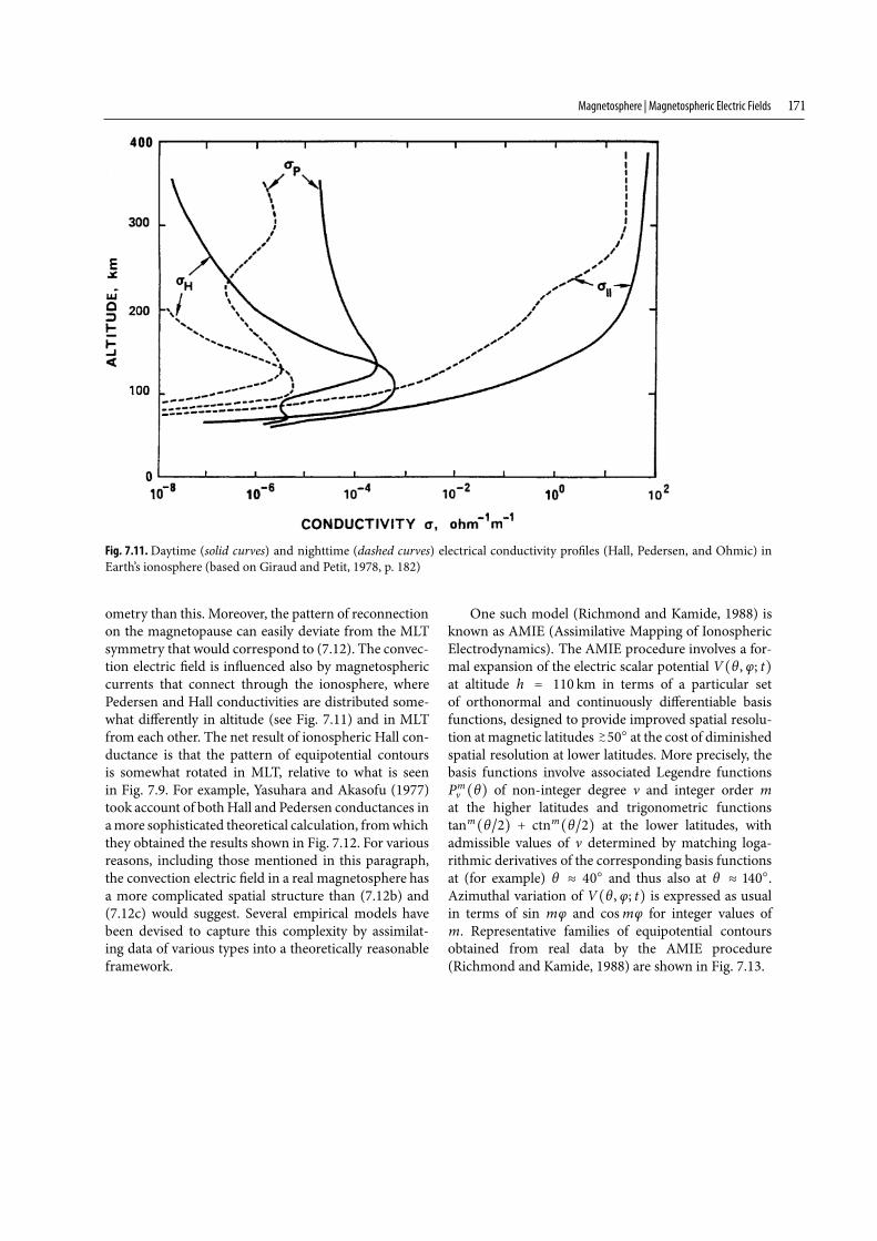
Fig. 7.11.Daytime (solid curves) and nighttime (dashed curves) electrical conductivity profiles (Hall, Pedersen, and Ohmic) inEarth’s ionosphere (based on Giraud and Petit, 1978, p. 182)

ometry than this. Moreover, the pattern of reconnectionon the magnetopause can easily deviate from the MLTsymmetry that would correspond to (7.12). The convec-tion electric field is influenced also by magnetosphericcurrents that connect through the ionosphere, wherePedersen and Hall conductivities are distributed some-what differently in altitude (see Fig. 7.11) and in MLTfrom each other. The net result of ionospheric Hall con-ductance is that the pattern of equipotential contoursis somewhat rotated in MLT, relative to what is seenin Fig. 7.9. For example, Yasuhara and Akasofu (1977)took account of bothHall and Pedersen conductances inamore sophisticated theoretical calculation, fromwhichthey obtained the results shown in Fig. 7.12. For variousreasons, including those mentioned in this paragraph,the convection electric field in a real magnetosphere hasa more complicated spatial structure than (7.12b) and(7.12c) would suggest. Several empirical models havebeen devised to capture this complexity by assimilat-ing data of various types into a theoretically reasonableframework.

One such model (Richmond and Kamide, 1988) isknown as AMIE (Assimilative Mapping of IonosphericElectrodynamics). The AMIE procedure involves a for-mal expansion of the electric scalar potential V(θ , φ; t)at altitude h = 110 km in terms of a particular setof orthonormal and continuously differentiable basisfunctions, designed to provide improved spatial resolu-tion atmagnetic latitudes �� � at the cost of diminishedspatial resolution at lower latitudes. More precisely, thebasis functions involve associated Legendre functionsPmν (θ) of non-integer degree ν and integer order m

at the higher latitudes and trigonometric functionstanm

(θ�) + ctnm(θ�) at the lower latitudes, with

admissible values of ν determined by matching loga-rithmic derivatives of the corresponding basis functionsat (for example) θ � � and thus also at θ � �.Azimuthal variation of V(θ , φ; t) is expressed as usualin terms of sin mφ and cosmφ for integer values ofm. Representative families of equipotential contoursobtained from real data by the AMIE procedure(Richmond and Kamide, 1988) are shown in Fig. 7.13.

M. Schulz

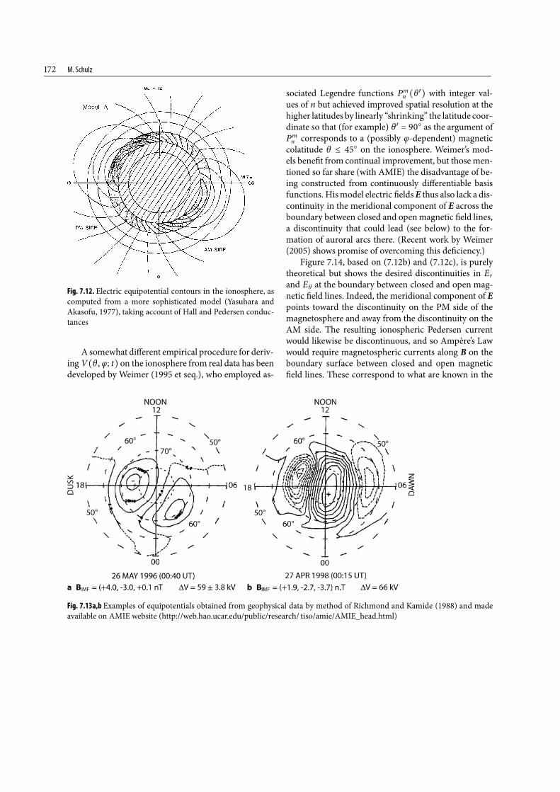
Fig. 7.12. Electric equipotential contours in the ionosphere, ascomputed from a more sophisticated model (Yasuhara andAkasofu, 1977), taking account of Hall and Pedersen conduc-tances

A somewhat different empirical procedure for deriv-ing V(θ , φ; t) on the ionosphere from real data has beendeveloped by Weimer (1995 et seq.), who employed as-

Fig. 7.13a,b Examples of equipotentials obtained from geophysical data by method of Richmond and Kamide (1988) and madeavailable on AMIE website (http://web.hao.ucar.edu/public/research/ tiso/amie/AMIE_head.html)

sociated Legendre functions Pmn (θ′) with integer val-

ues of n but achieved improved spatial resolution at thehigher latitudes by linearly “shrinking” the latitude coor-dinate so that (for example) θ′ = � as the argument ofPmn corresponds to a (possibly φ-dependent) magnetic

colatitude θ � � on the ionosphere. Weimer’s mod-els benefit from continual improvement, but those men-tioned so far share (with AMIE) the disadvantage of be-ing constructed from continuously differentiable basisfunctions. Hismodel electric fieldsE thus also lack a dis-continuity in the meridional component of E across theboundary between closed and openmagnetic field lines,a discontinuity that could lead (see below) to the for-mation of auroral arcs there. (Recent work by Weimer(2005) shows promise of overcoming this deficiency.)

Figure 7.14, based on (7.12b) and (7.12c), is purelytheoretical but shows the desired discontinuities in Erand Eθ at the boundary between closed and open mag-netic field lines. Indeed, the meridional component of Epoints toward the discontinuity on the PM side of themagnetosphere and away from the discontinuity on theAM side. The resulting ionospheric Pedersen currentwould likewise be discontinuous, and so Ampère’s Lawwould require magnetospheric currents along B on theboundary surface between closed and open magneticfield lines. These correspond to what are known in the

Magnetosphere | Magnetospheric Electric Fields

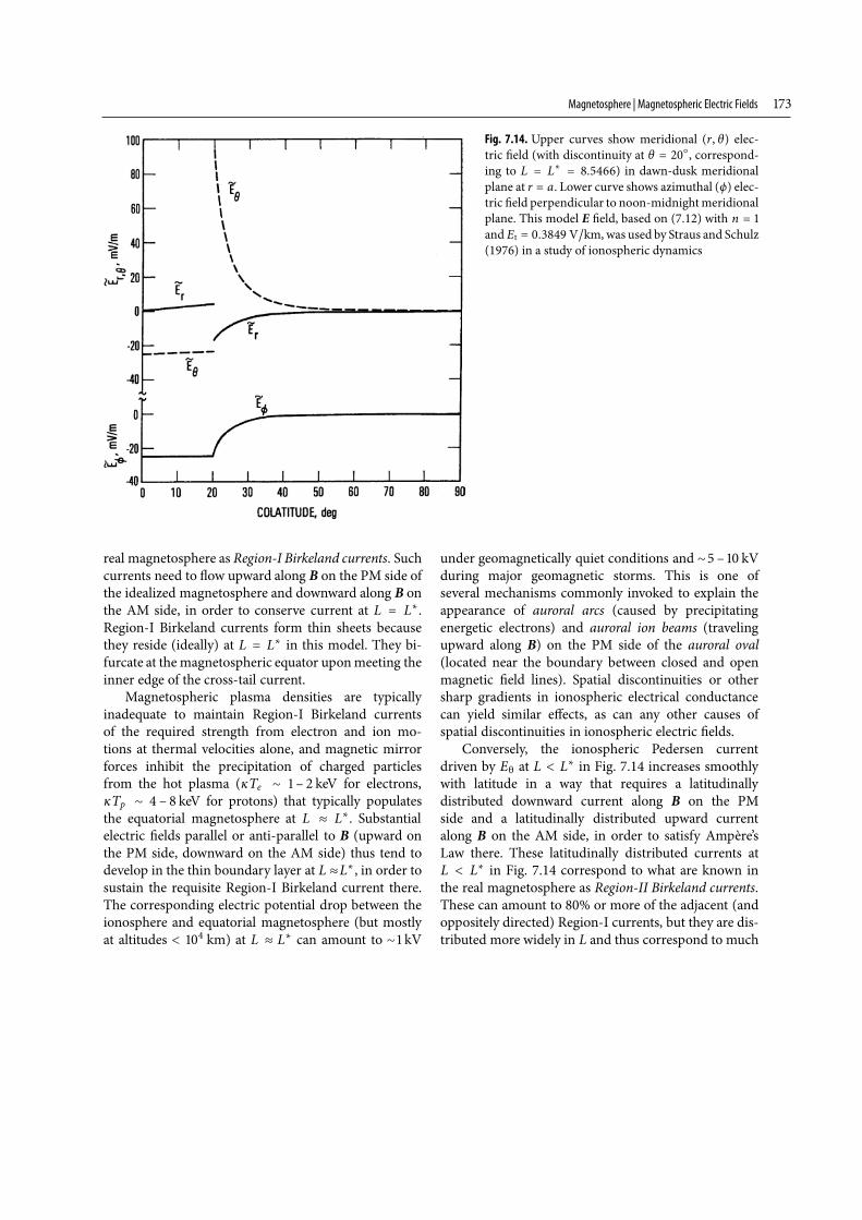
Fig. 7.14. Upper curves show meridional (r, θ) elec-tric field (with discontinuity at θ = �, correspond-ing to L = L� = .) in dawn-dusk meridionalplane at r = a. Lower curve shows azimuthal (ϕ) elec-tric field perpendicular to noon-midnightmeridionalplane. This model E field, based on (7.12) with n = and Et = . V�km, was used by Straus and Schulz(1976) in a study of ionospheric dynamics

real magnetosphere as Region-I Birkeland currents. Suchcurrents need to flow upward along B on the PM side ofthe idealized magnetosphere and downward along B onthe AM side, in order to conserve current at L = L�.Region-I Birkeland currents form thin sheets becausethey reside (ideally) at L = L� in this model. They bi-furcate at the magnetospheric equator uponmeeting theinner edge of the cross-tail current.

Magnetospheric plasma densities are typicallyinadequate to maintain Region-I Birkeland currentsof the required strength from electron and ion mo-tions at thermal velocities alone, and magnetic mirrorforces inhibit the precipitation of charged particlesfrom the hot plasma (κTe � – keV for electrons,κTp � – keV for protons) that typically populatesthe equatorial magnetosphere at L � L�. Substantialelectric fields parallel or anti-parallel to B (upward onthe PM side, downward on the AM side) thus tend todevelop in the thin boundary layer at L �L�, in order tosustain the requisite Region-I Birkeland current there.The corresponding electric potential drop between theionosphere and equatorial magnetosphere (but mostlyat altitudes < km) at L � L� can amount to � kV

under geomagnetically quiet conditions and � – kVduring major geomagnetic storms. This is one ofseveral mechanisms commonly invoked to explain theappearance of auroral arcs (caused by precipitatingenergetic electrons) and auroral ion beams (travelingupward along B) on the PM side of the auroral oval(located near the boundary between closed and openmagnetic field lines). Spatial discontinuities or othersharp gradients in ionospheric electrical conductancecan yield similar effects, as can any other causes ofspatial discontinuities in ionospheric electric fields.

Conversely, the ionospheric Pedersen currentdriven by Eθ at L < L� in Fig. 7.14 increases smoothlywith latitude in a way that requires a latitudinallydistributed downward current along B on the PMside and a latitudinally distributed upward currentalong B on the AM side, in order to satisfy Ampère’sLaw there. These latitudinally distributed currents atL < L� in Fig. 7.14 correspond to what are known inthe real magnetosphere as Region-II Birkeland currents.These can amount to % or more of the adjacent (andoppositely directed) Region-I currents, but they are dis-tributed more widely in L and thus correspond to much

M. Schulz

smaller current densities and much smaller parallel (toB) electric fields than are found in Region I. This laststatement reflects the smoothly monotonic variation ofEθ with latitude in Fig. 7.14 for L < L�, in contrast tothe discontinuity in Eθ encountered at L = L�. Iono-spheric Hall currents and their azimuthal variations, aswell as azimuthal variations of ionospheric Pedersencurrents, also contribute to the eventual distributionof magnetospheric Birkeland currents in L and φ, butintrinsic latitudinal variations of ionospheric Pedersencurrents account for the essential features noted above.In fact, the global distribution of Birkeland currentsis (for various reasons) more complicated than thepresent discussion might suggest. A famous empiricalstudy of Birkeland currents (deduced from satellite-magnetometer data) revealed the global pattern shownin Fig. 7.15. The anomalously large width of Region Iin Fig. 7.15 can be attributed in part to data-binning,as well as to temporal variations in the latitudes atwhich Region-I currents enter (AM) or leave (PM) theionosphere.

Finally, there is a need to consider induced electricfields associated with temporal variations of B. A sim-ple example is the electric field induced by allowing μEand/or b in (7.7a) or (7.7b) to vary with time. In these(axisymmetric) cases the induced electric field would begiven by

E = −φ(μE�r)[ + (r�b)] sin θ − φμE(r�b)b sin θ(7.14a)

or by

E = −φ(μE�r)[ − (r�b)] sin θ + φμE(r�b)b sin θ ,(7.14b)

respectively. The secular decrease (�.% per century)of the geomagnetic dipole moment μE is formally in-cluded in (7.14) but is unimportant formost calculationsofmagnetospheric particle dynamics. The usual sense inwhich μE varies with time is that temporal variations ofb (or of equivalent magnetospheric parameters) induceazimuthal currents in the ionosphere and/or in the Earthitself, so as to exclude (in first approximation) any ex-ternally imposed magnetic perturbation from an Earth-centered sphere of radius rc. Such an exclusion wouldrequire

μE�μE = −[ + (rc�b)]−(rc�b)(b�b) (7.15a)

in (7.14a) and

μE�μE = −[ − (rc�b)]−(rc�b)(b�b) (7.15b)

in (7.14b), respectively. The corresponding azimuthalsurface currents at r = rc would thus induce a dipolemoment ΔμE that may either add to or detract from thedipole moment associated with Earth’s main field.

The induced electric fieldsE specified by (7.14a) and(7.14b) are (of course) respectively perpendicular to B,as specified by (7.7a) and (7.7b). It is considered some-what of a paradigm inmagnetospheric physics that elec-tric fields (except in special cases such as auroral arcs)can be regarded as perpendicular toB for the purpose ofcalculating their spatial distributions. This is especiallyso for induced electric fields. In effect, any componentof E parallel to B is regarded as arising from a sepa-rate physical process. Using this paradigm, Fälthammar(1968) deduced the lowest-order generalization of (7.14)to models such as (7.1), in which the magnetic field B isnot axisymmetric. The result (valid up to second orderin r/b) is given by

E = − φ(r�b)b(a�b) g sin θ

− φ(r�b)b(a�b) g( sin θ − )� cos φ

− (r sin θ − θ cos θ)b(r�b)�(a�b) g sin φ(7.16)

if Earth-induction currents are neglected. Schulz andEviatar (1969) showed how to extend the calculation ofinduced electric fields term-by-term to ever higher or-der in r�b.

There is a philosophical question as to whether suchcalculations of induced electric fields are truly unique,since (it is argued) one can always add an electric field(perpendicular to B) that is the gradient of a scalarpotential dependent only on magnetic field-line labels(so that magnetic field lines are electric equipoten-tials). Since the curl of a gradient is always zero, it isargued that the resulting superposition still satisfiesMaxwell’s equations and (in particular) Faraday’s Lawof electromagnetic induction. The answer seems to bethat (7.14) has a certain “irreducible simplicity” thatwould be contaminated by arbitrarily adding anythingto it. As long as additional terms are generated outof necessity and by the same algorithm, to maintainE ċ B = and satisfy Maxwell’s equations to ever higher

Magnetosphere | Magnetospheric Charged Particles

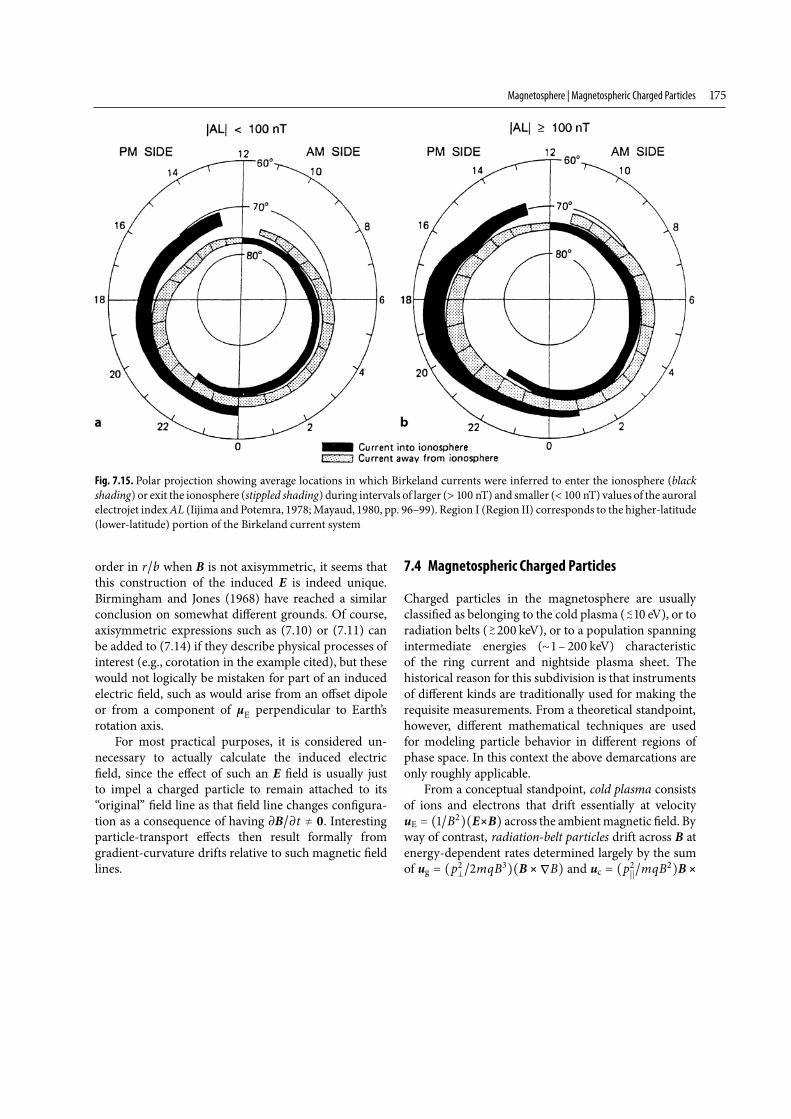
Fig. 7.15. Polar projection showing average locations in which Birkeland currents were inferred to enter the ionosphere (blackshading) or exit the ionosphere (stippled shading) during intervals of larger (� nT) and smaller (< nT) values of the auroralelectrojet indexAL (Iijima and Potemra, 1978;Mayaud, 1980, pp. 96–99). Region I (Region II) corresponds to the higher-latitude(lower-latitude) portion of the Birkeland current system

order in r�b when B is not axisymmetric, it seems thatthis construction of the induced E is indeed unique.Birmingham and Jones (1968) have reached a similarconclusion on somewhat different grounds. Of course,axisymmetric expressions such as (7.10) or (7.11) canbe added to (7.14) if they describe physical processes ofinterest (e.g., corotation in the example cited), but thesewould not logically be mistaken for part of an inducedelectric field, such as would arise from an offset dipoleor from a component of μE perpendicular to Earth’srotation axis.

For most practical purposes, it is considered un-necessary to actually calculate the induced electricfield, since the effect of such an E field is usually justto impel a charged particle to remain attached to its“original” field line as that field line changes configura-tion as a consequence of having ∂B�∂t � . Interestingparticle-transport effects then result formally fromgradient-curvature drifts relative to such magnetic fieldlines.

7.4 Magnetospheric Charged Particles

Charged particles in the magnetosphere are usuallyclassified as belonging to the cold plasma ( <� eV), or toradiation belts ( �� keV), or to a population spanningintermediate energies (� – keV) characteristicof the ring current and nightside plasma sheet. Thehistorical reason for this subdivision is that instrumentsof different kinds are traditionally used for making therequisite measurements. From a theoretical standpoint,however, different mathematical techniques are usedfor modeling particle behavior in different regions ofphase space. In this context the above demarcations areonly roughly applicable.

From a conceptual standpoint, cold plasma consistsof ions and electrons that drift essentially at velocityuE = (�B

)(E�B) across the ambientmagnetic field. Byway of contrast, radiation-belt particles drift across B atenergy-dependent rates determined largely by the sumof ug = (p

�mqB

)(B � ∇B) and uc = (p���mqB

)B �

M. Schulz

(∂B�∂s), known as the gradient-curvature drift veloc-ity, to which uE is an almost negligible addendum. (Thequantities p and p�� in ug and uc denote components ofparticle momentum p perpendicular and parallel to B.The mass m denotes relativistic mass if applicable, andthe direction of drift is determined by the sign of thecharge q. The coordinate s, usually measured frommin-ima in B, denotes distance along a magnetic field line.)The plasma sheet and ring current constitute a popula-tion of ions and electrons for which uE and ug + uc arecomparably important from a kinematical and dynami-cal standpoint.

Ions and electrons can also move along B. Such mo-tions are influenced by gravity and by centrifugal forcesassociated with curvature of E � B drift trajectories inthe case of cold plasma. They are influenced by com-ponents of E parallel to B for cold plasma and for plas-masheet particles in auroral arcs. They are influenced bymagnetic-mirror forces Fμ = −B(p

�mB)(B ċ ∇B) in

the case of plasmasheet, ring-current, and radiation-beltparticles.

The resulting motions, along and across B, can bebounded or not bounded within the magnetosphere.Particles for which the motion is (at least temporarily)bounded within the magnetosphere are said to betrapped. Those that escape into the ionosphere are saidto precipitate there. Some particles can escape across themagnetopause or into the tail, either because of driftsor because they are individually too energetic for themagnetosphere to contain them. Galactic cosmic raysand solar energetic particles typically belong to this lastcategory.

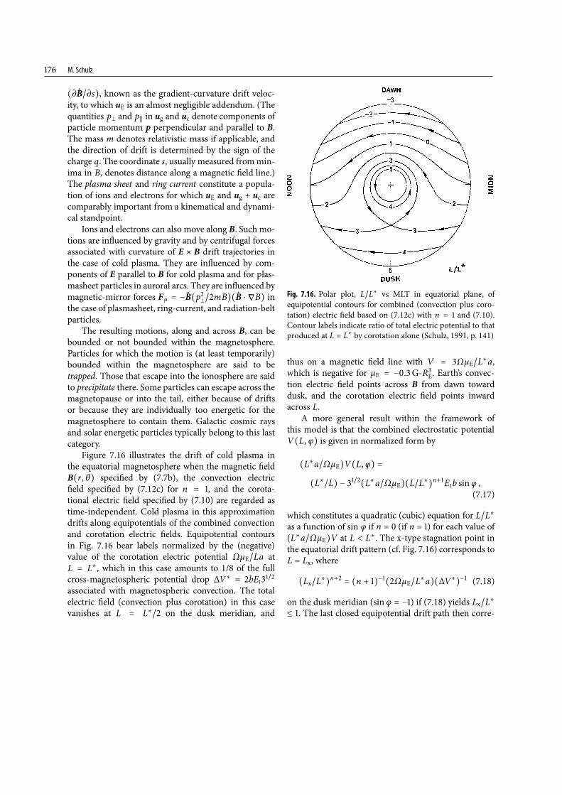
Figure 7.16 illustrates the drift of cold plasma inthe equatorial magnetosphere when the magnetic fieldB(r, θ) specified by (7.7b), the convection electricfield specified by (7.12c) for n = , and the corota-tional electric field specified by (7.10) are regarded astime-independent. Cold plasma in this approximationdrifts along equipotentials of the combined convectionand corotation electric fields. Equipotential contoursin Fig. 7.16 bear labels normalized by the (negative)value of the corotation electric potential ΩμE�La atL = L�, which in this case amounts to 1/8 of the fullcross-magnetospheric potential drop ΔV� = 2bEt3�associated with magnetospheric convection. The totalelectric field (convection plus corotation) in this casevanishes at L = L�� on the dusk meridian, and

Fig. 7.16. Polar plot, L�L� vs MLT in equatorial plane, ofequipotential contours for combined (convection plus coro-tation) electric field based on (7.12c) with n = and (7.10).Contour labels indicate ratio of total electric potential to thatproduced at L = L� by corotation alone (Schulz, 1991, p. 141)

thus on a magnetic field line with V = ΩμE�L�a,which is negative for μE = −.G-R

E. Earth’s convec-tion electric field points across B from dawn towarddusk, and the corotation electric field points inwardacross L.

A more general result within the framework ofthis model is that the combined electrostatic potentialV(L, φ) is given in normalized form by

(L�a�ΩμE)V(L, φ) =

(L��L) − �(L�a�ΩμE)(L�L�)n+Etb sin φ ,(7.17)

which constitutes a quadratic (cubic) equation for L�L�as a function of sin φ if n = (if n = ) for each value of(L�a�ΩμE)V at L < L�. The x-type stagnation point inthe equatorial drift pattern (cf. Fig. 7.16) corresponds toL = Lx, where

(Lx�L�)n+ = (n + )−(ΩμE�L�a)(ΔV�)− (7.18)

on the dusk meridian (sin φ = −) if (7.18) yields Lx�L�� . The last closed equipotential drift path then corre-

Magnetosphere | Magnetospheric Charged Particles

sponds to the value of (L�a�ΩμE)V specified by (7.17)at sin φ = − for this value of L�L�. In case (7.18) yieldsLx�L� (as might happen during geomagneticallyvery quiet time intervals) there is no x-type stagnationpoint, and the last closed equipotential drift path justgrazes the equatorial neutral line (r = b) at sin φ = −.The corresponding value of (L�a�ΩμE)V in this case isfound by specifying L�L� = .

The equatorial cold-plasma density N should varyas B along any equipotential drift path in Fig. 7.16. Therationale for this expectation follows from a simple cal-culation of ∇ ċ uE:

∇ ċ uE =∇ ċ [B−(E � B)]

= − B−[B ċ (∇ � E) − E ċ (∇ � B)]

− B−(E � B) ċ∇(B)

= − ∂(ln B)�∂t − (μ�B)(E ċ J)

− (εμ�B)∂(E

)�∂t − uE ċ∇(lnB) .(7.19)

If the magnetic field B is time-independent (such that∂B�∂t = ) and locally current-free (such that J = ),and if the displacement current is neglected as usual,then ∇ � E = ∇ � B = . In this case it follows fromthe continuity equation (∂N�∂t) +∇ ċ (uEN) = that

dN�dt = (∂N�∂t) + (uE ċ∇N) = −N(∇ ċ uE) (7.20a)

and thus from (7.19) that

d(lnN)�dt − d(lnB)�dt = d ln(N�B

)�dt = .(7.20b)

It follows that (except for in situ production or loss, andexcept for any transport of cold plasma alongB) the ratioN�B should remain constant along any E � B drift tra-jectory. Except perhaps for seasonal or dipole-tilt effects,the component of cold-plasma velocity along B and itsfirst derivative with respect to s should vanish at or nearthe magnetic equator, thereby removing the reservationabout plasma transport along B.

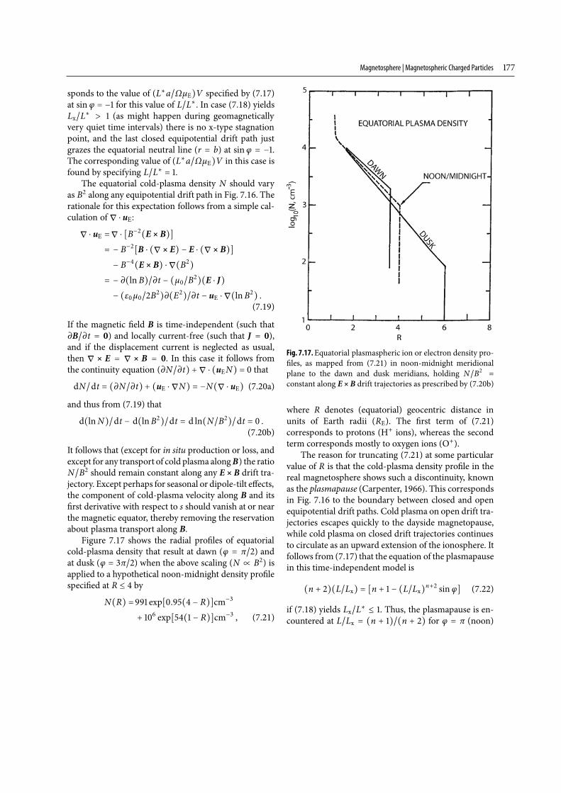
Figure 7.17 shows the radial profiles of equatorialcold-plasma density that result at dawn (φ = π�) andat dusk (φ = π�) when the above scaling (N � B) isapplied to a hypothetical noon-midnight density profilespecified at R � by

N(R) = exp[.( − R)]cm−

+ exp[( − R)]cm− , (7.21)

Fig. 7.17.Equatorial plasmaspheric ion or electron density pro-files, as mapped from (7.21) in noon-midnight meridionalplane to the dawn and dusk meridians, holding N�B

=

constant along E �B drift trajectories as prescribed by (7.20b)

where R denotes (equatorial) geocentric distance inunits of Earth radii (RE). The first term of (7.21)corresponds to protons (H+ ions), whereas the secondterm corresponds mostly to oxygen ions (O+).

The reason for truncating (7.21) at some particularvalue of R is that the cold-plasma density profile in thereal magnetosphere shows such a discontinuity, knownas the plasmapause (Carpenter, 1966). This correspondsin Fig. 7.16 to the boundary between closed and openequipotential drift paths. Cold plasma on open drift tra-jectories escapes quickly to the dayside magnetopause,while cold plasma on closed drift trajectories continuesto circulate as an upward extension of the ionosphere. Itfollows from (7.17) that the equation of the plasmapausein this time-independent model is

(n + )(L�Lx) = [n + − (L�Lx)n+ sin φ] (7.22)

if (7.18) yields Lx�L� � . Thus, the plasmapause is en-countered at L�Lx = (n + )�(n + ) for φ = π (noon)

M. Schulz

and for φ = (midnight), and so truncation of the noon-midnight density profile at R = in Fig. 7.17 corre-sponds to truncation of the dusk (φ = π�) densityprofile at R � . The plasmapause maps to higher lat-itudes along magnetic field lines, as specified by (7.8b)in this model. The region of higher cold-plasma den-sity enclosed by the plasmapause is known as the plas-masphere. The cold-plasmadensityN typically increaseswith latitude (i.e., with decreasing r) along any field lineinside the plasmasphere, so as to connect smoothly withthe corresponding topside ionospheric plasma-densityprofile at an altitude � km.

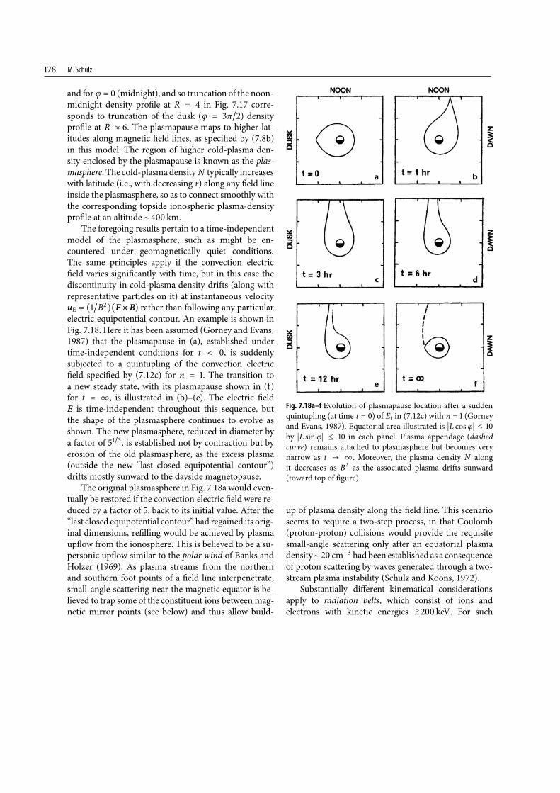
The foregoing results pertain to a time-independentmodel of the plasmasphere, such as might be en-countered under geomagnetically quiet conditions.The same principles apply if the convection electricfield varies significantly with time, but in this case thediscontinuity in cold-plasma density drifts (along withrepresentative particles on it) at instantaneous velocityuE = (�B

)(E �B) rather than following any particularelectric equipotential contour. An example is shown inFig. 7.18. Here it has been assumed (Gorney and Evans,1987) that the plasmapause in (a), established undertime-independent conditions for t < , is suddenlysubjected to a quintupling of the convection electricfield specified by (7.12c) for n = . The transition toa new steady state, with its plasmapause shown in (f)for t = �, is illustrated in (b)–(e). The electric fieldE is time-independent throughout this sequence, butthe shape of the plasmasphere continues to evolve asshown. The new plasmasphere, reduced in diameter bya factor of �, is established not by contraction but byerosion of the old plasmasphere, as the excess plasma(outside the new “last closed equipotential contour”)drifts mostly sunward to the dayside magnetopause.

The original plasmasphere in Fig. 7.18a would even-tually be restored if the convection electric field were re-duced by a factor of 5, back to its initial value. After the“last closed equipotential contour” had regained its orig-inal dimensions, refilling would be achieved by plasmaupflow from the ionosphere. This is believed to be a su-personic upflow similar to the polar wind of Banks andHolzer (1969). As plasma streams from the northernand southern foot points of a field line interpenetrate,small-angle scattering near the magnetic equator is be-lieved to trap some of the constituent ions between mag-netic mirror points (see below) and thus allow build-

Fig. 7.18a–f Evolution of plasmapause location after a suddenquintupling (at time t = ) of Et in (7.12c) with n = (Gorneyand Evans, 1987). Equatorial area illustrated is �L cosφ� � by �L sin φ� � in each panel. Plasma appendage (dashedcurve) remains attached to plasmasphere but becomes verynarrow as t . Moreover, the plasma density N alongit decreases as B as the associated plasma drifts sunward(toward top of figure)

up of plasma density along the field line. This scenarioseems to require a two-step process, in that Coulomb(proton-proton) collisions would provide the requisitesmall-angle scattering only after an equatorial plasmadensity� cm− had been established as a consequenceof proton scattering by waves generated through a two-stream plasma instability (Schulz and Koons, 1972).

Substantially different kinematical considerationsapply to radiation belts, which consist of ions andelectrons with kinetic energies �

� keV. For such

Magnetosphere | Magnetospheric Charged Particles

particles the main drifts are ug = (p�mqB

)(B�∇B)and uc = (p

���mqB

)B � (∂B�∂s), known as gradientand curvature drifts, rather than uE = (�B

)(E � B).The gradient-curvature drift in the geomagnetic field iseastward for electrons (with charge q < ) and westwardfor positive ions (q ). The logic of gradient driftis that particles of magnetic moment μ = p

�mB

experience a net force Fg = −μ∇B as they gyrate in aninhomogeneous B field, much as they experience anelectric force qE in the presence of an electric field. Theresulting drift velocity ug = (μ�qB

)(B � ∇B) trans-verse to B is thus found by substituting E � −(μ�q)∇Bin the expression for uE = (�B

)(E � B). Similarly,a charged particle with velocity component p���malong B, as its center of gyration “tries” to follow themagnetic field line, must experience a “centrifugal”force Fc = −(p

���m)(∂B�∂s) in consequence of the field

line’s local curvature ∂B�∂s. The resulting drift velocityuc = (p

���mqB

)B � (∂B�∂s) is found by substitutingE � −(p

���mq)(∂B�∂s) in the above expression for uE.

A particle’s magnetic moment μ = p�γmB is

closely related to a quantity M = p�mB known as its

first adiabatic invariant, where γ � m�m is the ratio ofrelativistic mass (m) to rest mass (m). The first invari-ant M is a conserved quantity except for processes thatinterfere with particle gyration (at frequency Ω�π =

qB�πm) about the local magnetic field line, essentiallybecause M is proportional to the canonical action in-tegral (see below) associated with particle gyration. Itfollows that a particle’s value of p

(= mMB) varies

in proportion to the value of B at its center of gyrationunder these conditions. Since electric fields parallel toB are considered negligible for particles with radiation-belt energies, a particle’s component of momentum par-allel to B is given by

p�� � (p − p)

�= (p − mMB)�

= p[ − (B�Bm)]� , (7.23)

where Bm (= p�mM) is known as the mirror-pointfield because it is the value of B required tomake p�� = .

A charged particle is thus (in principle) trapped be-tween points at which B = Bm along a magnetic fieldline, and the motion of its center of gyration betweensuchmirror points is known as bouncemotion. The timerequired for a particle’s guiding center (as the center ofgyration is known because it tends to follow the local

magnetic field line) to travel from either mirror point tothe other and back is known as the particle’s bounce pe-riod. If the particle’s mirror points are sufficiently nearthe magnetic equator (locus of minima in B along fieldlines), then the bounce motion is like that of a simpleharmonic oscillator, and the bounce frequency is givenby Ω�π = (�π)(M�γm)

�(∂B�∂s)� , where the

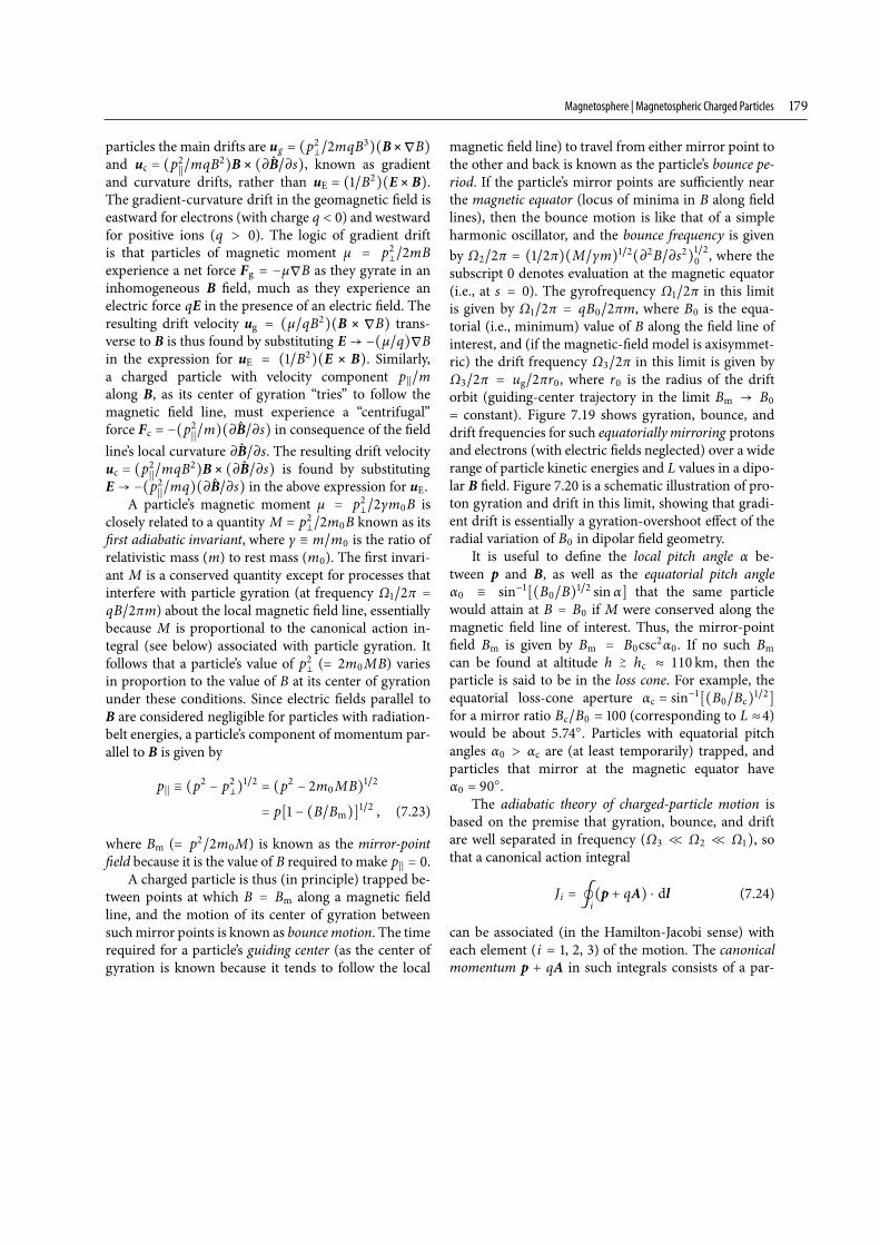
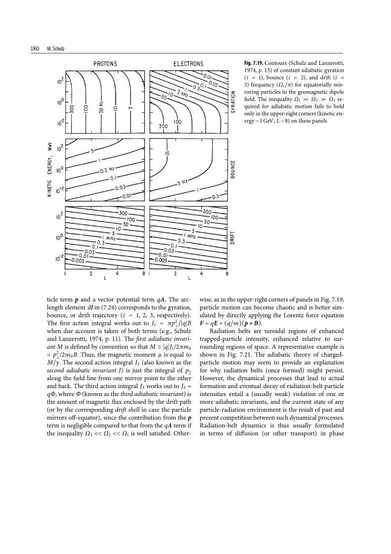
subscript 0 denotes evaluation at the magnetic equator(i.e., at s = ). The gyrofrequency Ω�π in this limitis given by Ω�π = qB�πm, where B is the equa-torial (i.e., minimum) value of B along the field line ofinterest, and (if the magnetic-field model is axisymmet-ric) the drift frequency Ω�π in this limit is given byΩ�π = ug�πr, where r is the radius of the driftorbit (guiding-center trajectory in the limit Bm � B= constant). Figure 7.19 shows gyration, bounce, anddrift frequencies for such equatoriallymirroring protonsand electrons (with electric fields neglected) over a widerange of particle kinetic energies and L values in a dipo-lar B field. Figure 7.20 is a schematic illustration of pro-ton gyration and drift in this limit, showing that gradi-ent drift is essentially a gyration-overshoot effect of theradial variation of B in dipolar field geometry.

It is useful to define the local pitch angle α be-tween p and B, as well as the equatorial pitch angleα � sin−[(B�B)� sin α] that the same particlewould attain at B = B if M were conserved along themagnetic field line of interest. Thus, the mirror-pointfield Bm is given by Bm = Bcscα. If no such Bmcan be found at altitude h �

� hc � 110 km, then theparticle is said to be in the loss cone. For example, theequatorial loss-cone aperture αc = sin−[(B�Bc)

�]

for a mirror ratio Bc�B = (corresponding to L �)would be about .�. Particles with equatorial pitchangles α αc are (at least temporarily) trapped, andparticles that mirror at the magnetic equator haveα = �.

The adiabatic theory of charged-particle motion isbased on the premise that gyration, bounce, and driftare well separated in frequency (Ω ll Ω ll Ω), sothat a canonical action integral

Ji = �

i(p + qA) ċ dl (7.24)

can be associated (in the Hamilton-Jacobi sense) witheach element (i = , 2, 3) of the motion. The canonicalmomentum p + qA in such integrals consists of a par-

M. Schulz

Fig. 7.19. Contours (Schulz and Lanzerotti,1974, p. 13) of constant adiabatic gyration(i = ), bounce (i = ), and drift (i =) frequency (Ωi�π) for equatorially mir-roring particles in the geomagnetic dipolefield. The inequality Ω � Ω � Ω re-quired for adiabatic motion fails to holdonly in the upper-right corners (kinetic en-ergy � GeV, L �) on these panels

ticle term p and a vector potential term qA. The arc-length element dl in (7.24) corresponds to the gyration,bounce, or drift trajectory (i = , 2, 3, respectively).The first action integral works out to J = πp

��q�B

when due account is taken of both terms (e.g., Schulzand Lanzerotti, 1974, p. 11). The first adiabatic invari-ant M is defined by convention so that M � �q�J/2πm= p

/2mB. Thus, the magnetic moment μ is equal to

M�γ. The second action integral J (also known as thesecond adiabatic invariant J) is just the integral of p��along the field line from one mirror point to the otherand back. The third action integral J works out to J =qΦ, where Φ (known as the third adiabatic invariant) isthe amount of magnetic flux enclosed by the drift path(or by the corresponding drift shell in case the particlemirrors off-equator), since the contribution from the pterm is negligible compared to that from the qA term ifthe inequality Ω << Ω << Ω is well satisfied. Other-

wise, as in the upper-right corners of panels in Fig. 7.19,particle motion can become chaotic and is better sim-ulated by directly applying the Lorentz force equationF = qE + (q�m)(p � B).

Radiation belts are toroidal regions of enhancedtrapped-particle intensity, enhanced relative to sur-rounding regions of space. A representative example isshown in Fig. 7.21. The adiabatic theory of charged-particle motion may seem to provide an explanationfor why radiation belts (once formed) might persist.However, the dynamical processes that lead to actualformation and eventual decay of radiation-belt particleintensities entail a (usually weak) violation of one ormore adiabatic invariants, and the current state of anyparticle-radiation environment is the result of past andpresent competition between such dynamical processes.Radiation-belt dynamics is thus usually formulatedin terms of diffusion (or other transport) in phase

Magnetosphere | Magnetospheric Charged Particles

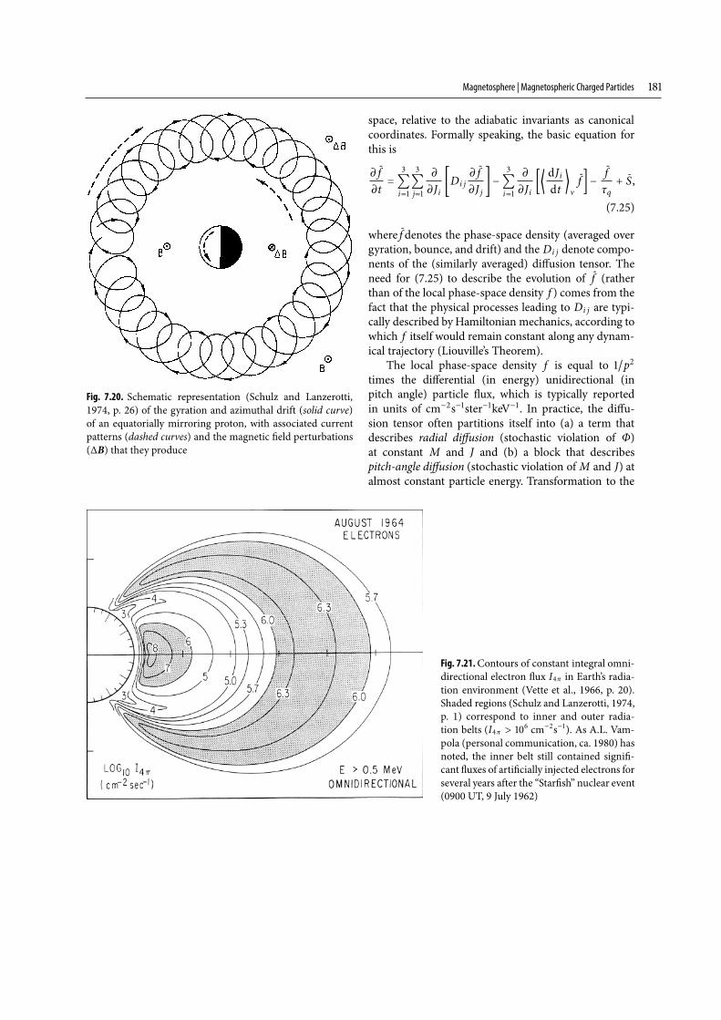
Fig. 7.20. Schematic representation (Schulz and Lanzerotti,1974, p. 26) of the gyration and azimuthal drift (solid curve)of an equatorially mirroring proton, with associated currentpatterns (dashed curves) and the magnetic field perturbations(ΔB) that they produce

Fig. 7.21.Contours of constant integral omni-directional electron flux Iπ in Earth’s radia-tion environment (Vette et al., 1966, p. 20).Shaded regions (Schulz and Lanzerotti, 1974,p. 1) correspond to inner and outer radia-tion belts (Iπ � cm−s−). As A.L. Vam-pola (personal communication, ca. 1980) hasnoted, the inner belt still contained signifi-cant fluxes of artificially injected electrons forseveral years after the “Starfish” nuclear event(0900 UT, 9 July 1962)

space, relative to the adiabatic invariants as canonicalcoordinates. Formally speaking, the basic equation forthis is

∂ f∂t

=

�

i=

�

j=

∂∂Ji

�Di j∂ f∂J j

�−

�

i=

∂∂Ji

��

dJidt

�

νf�−

fτq

+ S,

(7.25)

where f denotes the phase-space density (averaged overgyration, bounce, and drift) and the Di j denote compo-nents of the (similarly averaged) diffusion tensor. Theneed for (7.25) to describe the evolution of f (ratherthan of the local phase-space density f ) comes from thefact that the physical processes leading to Di j are typi-cally described byHamiltonian mechanics, according towhich f itself would remain constant along any dynam-ical trajectory (Liouville’s Theorem).

The local phase-space density f is equal to �ptimes the differential (in energy) unidirectional (inpitch angle) particle flux, which is typically reportedin units of cm−s−ster−keV− . In practice, the diffu-sion tensor often partitions itself into (a) a term thatdescribes radial diffusion (stochastic violation of Φ)at constant M and J and (b) a block that describespitch-angle diffusion (stochastic violation of M and J) atalmost constant particle energy. Transformation to the

M. Schulz

more convenient variables L � πμE�aΦ and x � cos αthen yields

�

i=

�

j=

∂∂Ji

�Di j∂ f∂J j

� = L∂∂L

�

DLL

L∂ f∂L

�

M , J

+

Ω

x∂∂x

�

xDxx

Ω

∂ f∂x

�

p,L(7.26)

after due account is taken of the requisite Jacobianfactors. It has been common in various applications ofradiation-belt physics to regard pitch-angle diffusion ei-ther as negligible, or as sufficient to impel attainment ofthe lowest eigenmode g(x) of the pitch-angle diffusionoperator in (7.26), or as strong enough to randomize theequatorial pitch angle α on the half-bounce time scale(π�Ω), so as to make the pitch-angle distribution fullyisotropic at scalar-momentum (p) values of interest.Under approximations such as these it is permissible toreplace the pitch-angle diffusion operator in (7.26) byan L-dependent factor −λ, and thus the correspondingterm in (7.26) by −λ f , with λ = or λ (lowest eigen-value of the pitch-angle diffusion operator) orΩ�π (fora particle in the loss cone), whichever is appropriate tothe underlying assumption about Dxx . Even for a par-ticle in the loss cone, the effective loss rate is limited totwice the bounce frequency because a particle requiresa quarter bounce period to reach the atmosphere fromthe equator, and the equatorial pitch-angle distributionthen requires another quarter bounce period to recog-nize that the particle has been lost (e.g., Lyons, 1973).

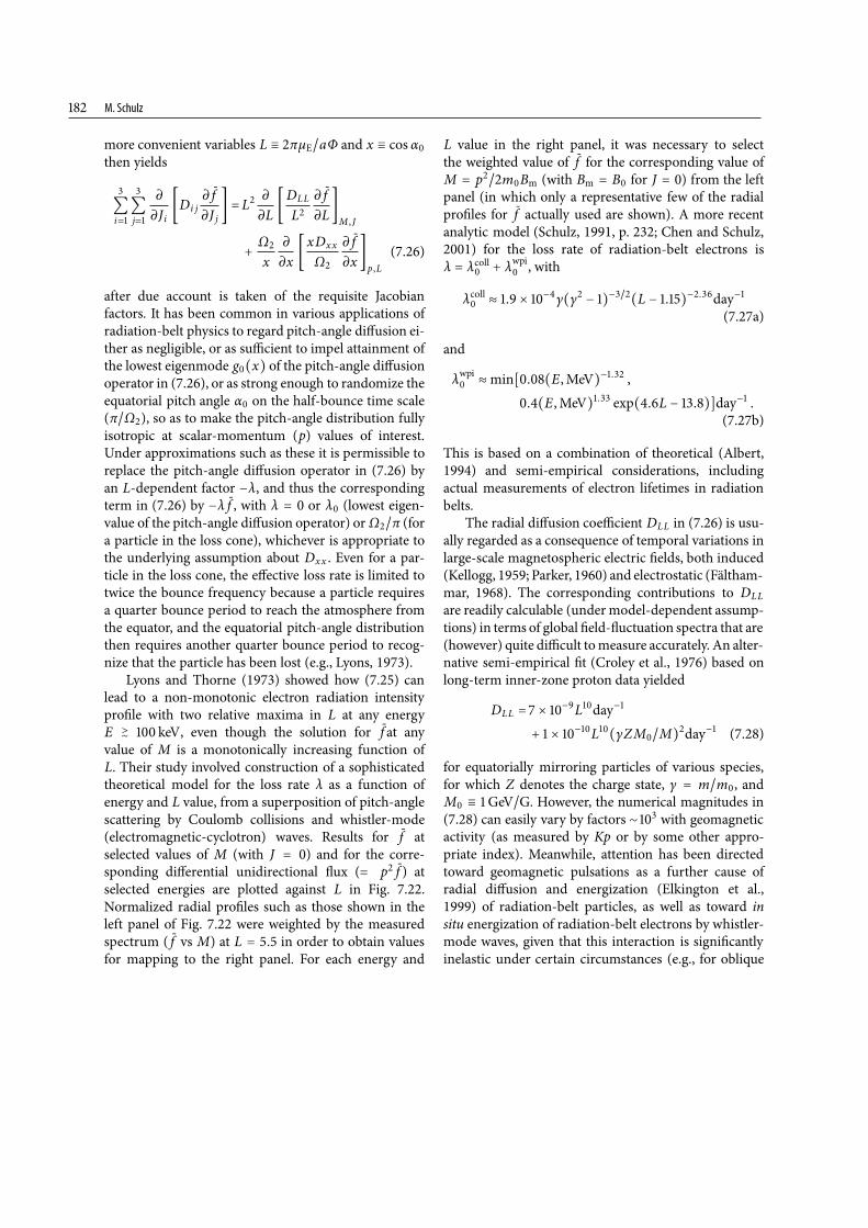
Lyons and Thorne (1973) showed how (7.25) canlead to a non-monotonic electron radiation intensityprofile with two relative maxima in L at any energyE �� keV, even though the solution for f at any

value of M is a monotonically increasing function ofL. Their study involved construction of a sophisticatedtheoretical model for the loss rate λ as a function ofenergy and L value, from a superposition of pitch-anglescattering by Coulomb collisions and whistler-mode(electromagnetic-cyclotron) waves. Results for f atselected values of M (with J = ) and for the corre-sponding differential unidirectional flux (= p f ) atselected energies are plotted against L in Fig. 7.22.Normalized radial profiles such as those shown in theleft panel of Fig. 7.22 were weighted by the measuredspectrum ( f vs M) at L = . in order to obtain valuesfor mapping to the right panel. For each energy and

L value in the right panel, it was necessary to selectthe weighted value of f for the corresponding value ofM = p�mBm (with Bm = B for J = ) from the leftpanel (in which only a representative few of the radialprofiles for f actually used are shown). A more recentanalytic model (Schulz, 1991, p. 232; Chen and Schulz,2001) for the loss rate of radiation-belt electrons isλ = λcoll + λwpi , with

λcoll � . � −γ(γ − )−�(L − .)−.day−

(7.27a)

and

λwpi �min[.(E,MeV)−. ,

.(E,MeV). exp(.L − .)]day− .(7.27b)

This is based on a combination of theoretical (Albert,1994) and semi-empirical considerations, includingactual measurements of electron lifetimes in radiationbelts.

The radial diffusion coefficient DLL in (7.26) is usu-ally regarded as a consequence of temporal variations inlarge-scale magnetospheric electric fields, both induced(Kellogg, 1959; Parker, 1960) and electrostatic (Fältham-mar, 1968). The corresponding contributions to DLLare readily calculable (undermodel-dependent assump-tions) in terms of global field-fluctuation spectra that are(however) quite difficult tomeasure accurately. An alter-native semi-empirical fit (Croley et al., 1976) based onlong-term inner-zone proton data yielded

DLL = � −Lday−

+ � −L(γZM�M)

day− (7.28)

for equatorially mirroring particles of various species,for which Z denotes the charge state, γ = m�m, andM � GeV�G. However, the numerical magnitudes in(7.28) can easily vary by factors � with geomagneticactivity (as measured by Kp or by some other appro-priate index). Meanwhile, attention has been directedtoward geomagnetic pulsations as a further cause ofradial diffusion and energization (Elkington et al.,1999) of radiation-belt particles, as well as toward insitu energization of radiation-belt electrons by whistler-mode waves, given that this interaction is significantlyinelastic under certain circumstances (e.g., for oblique

Magnetosphere | Magnetospheric Charged Particles

Fig. 7.22a,bPredicted steady-state profiles (a) of phase-space density f at constant M, obtained (Lyons and Thorne, 1973; Schulz,1975, p. 500) from a model similar to (7.25)–(7.28) and normalized to a common value at L = .; and predicted differentialparticle flux (b) at specified kinetic energies, normalized by prescribing the measured energy spectrum at L = . (Lyons andThorne, 1973)

wave propagation, and where the wave frequency ω�πmatches the relativistic electron gyrofrequency).

Additional terms on the RHS of (7.25) describefrictional forces (denoted by subscript ν) such asCoulomb drag, in situ loss processes such as chargeexchange (characterized by lifetime τq), and distributedsources (characterized by S) associated (for example)with beta decay of neutrons emitted from the upperatmosphere because of cosmic-ray bombardment.Charge exchange can also provide a distributed sourcefor ions of a particular charge state (e.g., for He+) atthe expense of an adjacent charge state (e.g., He++) orthrough the ionization of fast energetic neutral atoms.

The radial diffusion coefficient specified by (7.28)cannot be extrapolated indefinitely toward small valuesof M�M, since a factor [ + (Ωτ)−]− not shown in(7.28) imposes an upper bound � � −Lday− on thesecond term. The parameter τ (� s) in this factorrepresents the characteristic time for exponential decay

of impulses in the convection electric field, onwhich thispart of the model for radial diffusion is based. The resultquoted in (7.28) corresponds to Ωτ 1, but values ofM for which (7.28) thereby fails (M <

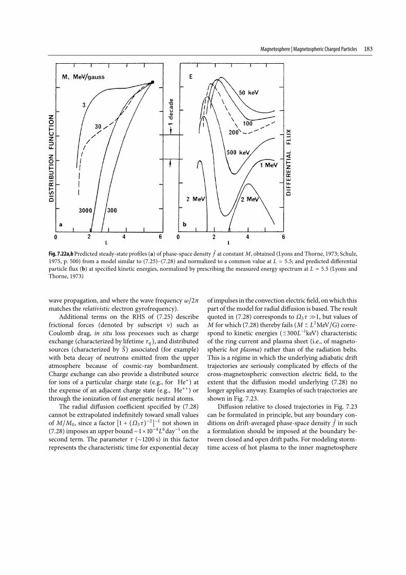
� LMeV�G) corre-spond to kinetic energies ( <� L−keV) characteristicof the ring current and plasma sheet (i.e., of magneto-spheric hot plasma) rather than of the radiation belts.This is a régime in which the underlying adiabatic drifttrajectories are seriously complicated by effects of thecross-magnetospheric convection electric field, to theextent that the diffusion model underlying (7.28) nolonger applies anyway. Examples of such trajectories areshown in Fig. 7.23.

Diffusion relative to closed trajectories in Fig. 7.23can be formulated in principle, but any boundary con-ditions on drift-averaged phase-space density f in sucha formulation should be imposed at the boundary be-tween closed and open drift paths. For modeling storm-time access of hot plasma to the inner magnetosphere

M. Schulz

Magnetosphere | Magnetospheric Charged Particles

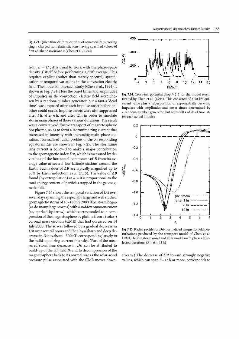
Fig. 7.23.Quiet-time drift trajectories of equatorially mirroringsingly charged nonrelativistic ions having specified values offirst adiabatic invariant μ (Chen et al., 1994)

from L = L�, it is usual to work with the phase-spacedensity f itself before performing a drift average. Thisrequires explicit (rather than merely spectral) specifi-cation of temporal variations in the convection electricfield. Themodel for one such study (Chen et al., 1994) isshown in Fig. 7.24. Here the onset times and amplitudesof impulses in the convection electric field were cho-sen by a random-number generator, but a 600-s “deadtime” was imposed after each impulse onset before an-other could occur. Impulse onsets were also suppressedafter h, after h, and after h in order to simulatestormmain phases of these various durations. The resultwas a convective/diffusive transport of magnetospherichot plasma, so as to form a stormtime ring current thatincreased in intensity with increasing main-phase du-ration. Normalized radial profiles of the correspondingequatorial ΔB are shown in Fig. 7.25. The stormtimering current is believed to make a major contributionto the geomagnetic index Dst, which is measured by de-viations of the horizontal component of B from its av-erage value at several low-latitude stations around theEarth. Such values of ΔB are typically magnified up to% by Earth induction, as in (7.15). The value of ΔBfound (by extrapolation) at R = is proportional to thetotal energy content of particles trapped in the geomag-netic field.

Figure 7.26 shows the temporal variation ofDst oversevendays spanning the especially large andwell studiedgeomagnetic storm of 15–16 July 2000. The storm began(as domany large storms) with a sudden commencement(sc, marked by arrow), which corresponded to a com-pression of themagnetosphere by plasma from a (solar-)coronal mass ejection (CME) that had occurred on 14July 2000. The sc was followed by a gradual decrease inDst over several hours and then by a sharp and deep de-crease inDst to about − nT, corresponding largely tothe build-up of ring-current intensity. (Part of the mea-sured stormtime decrease in Dst can be attributed tobuild-up of the tail field Bt and to decompression of themagnetosphere back to its normal size as the solar-windpressure pulse associated with the CME moves down-

Fig. 7.24. Cross-tail potential drop V(t) for the model stormtreated by Chen et al. (1994). This consisted of a 50-kV qui-escent value plus a superposition of exponentially decayingimpulses with amplitudes and onset times determined bya random-number generator, but with s of dead time af-ter each actual impulse

Fig. 7.25.Radial profiles of Dst-normalized magnetic-field per-turbations produced by the transport model of Chen et al.(1994), before storm onset and after model main phases of se-lected durations ( h, h, h)

stream.) The decrease of Dst toward strongly negativevalues, which can span – h or more, corresponds to

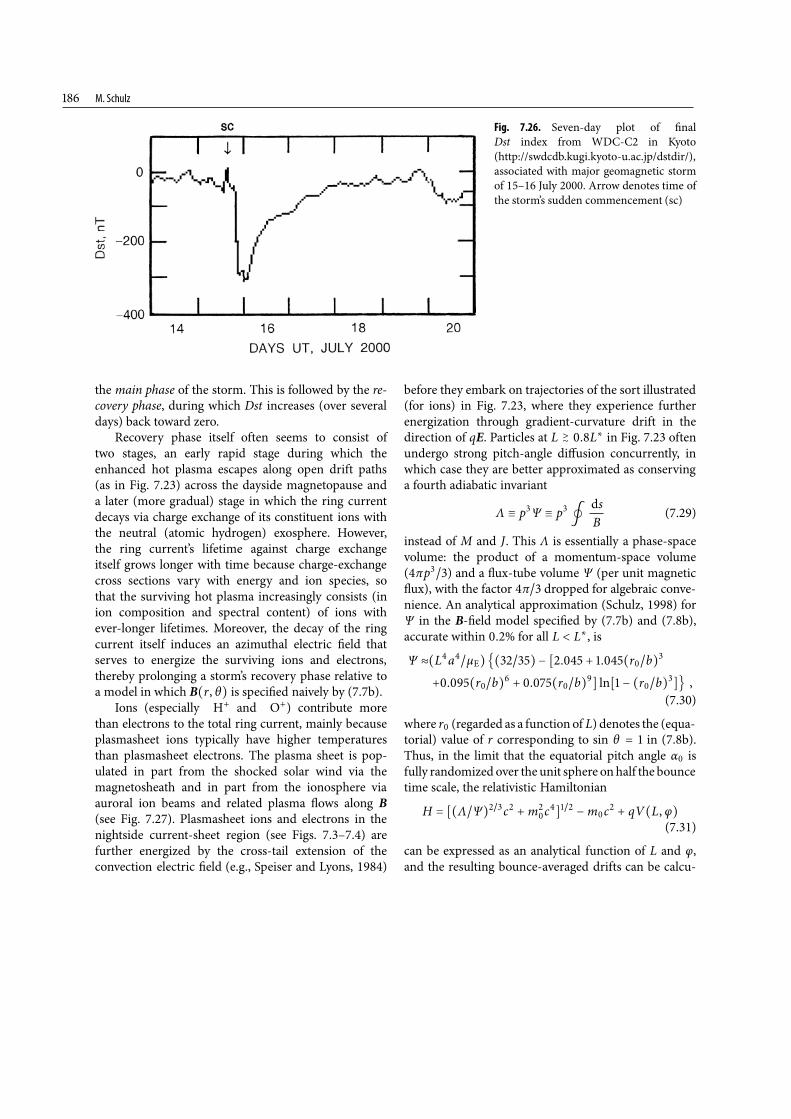
M. Schulz

Fig. 7.26. Seven-day plot of finalDst index from WDC-C2 in Kyoto(http://swdcdb.kugi.kyoto-u.ac.jp/dstdir/),associated with major geomagnetic stormof 15–16 July 2000. Arrow denotes time ofthe storm’s sudden commencement (sc)

the main phase of the storm. This is followed by the re-covery phase, during which Dst increases (over severaldays) back toward zero.

Recovery phase itself often seems to consist oftwo stages, an early rapid stage during which theenhanced hot plasma escapes along open drift paths(as in Fig. 7.23) across the dayside magnetopause anda later (more gradual) stage in which the ring currentdecays via charge exchange of its constituent ions withthe neutral (atomic hydrogen) exosphere. However,the ring current’s lifetime against charge exchangeitself grows longer with time because charge-exchangecross sections vary with energy and ion species, sothat the surviving hot plasma increasingly consists (inion composition and spectral content) of ions withever-longer lifetimes. Moreover, the decay of the ringcurrent itself induces an azimuthal electric field thatserves to energize the surviving ions and electrons,thereby prolonging a storm’s recovery phase relative toa model in which B(r, θ) is specified naively by (7.7b).

Ions (especially H+ and O+) contribute morethan electrons to the total ring current, mainly becauseplasmasheet ions typically have higher temperaturesthan plasmasheet electrons. The plasma sheet is pop-ulated in part from the shocked solar wind via themagnetosheath and in part from the ionosphere viaauroral ion beams and related plasma flows along B(see Fig. 7.27). Plasmasheet ions and electrons in thenightside current-sheet region (see Figs. 7.3–7.4) arefurther energized by the cross-tail extension of theconvection electric field (e.g., Speiser and Lyons, 1984)

before they embark on trajectories of the sort illustrated(for ions) in Fig. 7.23, where they experience furtherenergization through gradient-curvature drift in thedirection of qE. Particles at L �� .L� in Fig. 7.23 oftenundergo strong pitch-angle diffusion concurrently, inwhich case they are better approximated as conservinga fourth adiabatic invariant

Λ � pΨ � p�

dsB

(7.29)

instead of M and J. This Λ is essentially a phase-spacevolume: the product of a momentum-space volume(πp�) and a flux-tube volume Ψ (per unit magneticflux), with the factor π� dropped for algebraic conve-nience. An analytical approximation (Schulz, 1998) forΨ in the B-field model specified by (7.7b) and (7.8b),accurate within .% for all L < L�, is

Ψ �(La�μE) (�) − [. + .(r�b)

+.(r�b) + .(r�b)] ln[ − (r�b)]! ,(7.30)

where r (regarded as a function of L) denotes the (equa-torial) value of r corresponding to sin θ = in (7.8b).Thus, in the limit that the equatorial pitch angle α isfully randomized over the unit sphere onhalf the bouncetime scale, the relativistic Hamiltonian

H = [(Λ�Ψ)�c +mc

]

�−mc + qV(L, φ)

(7.31)

can be expressed as an analytical function of L and φ,and the resulting bounce-averaged drifts can be calcu-

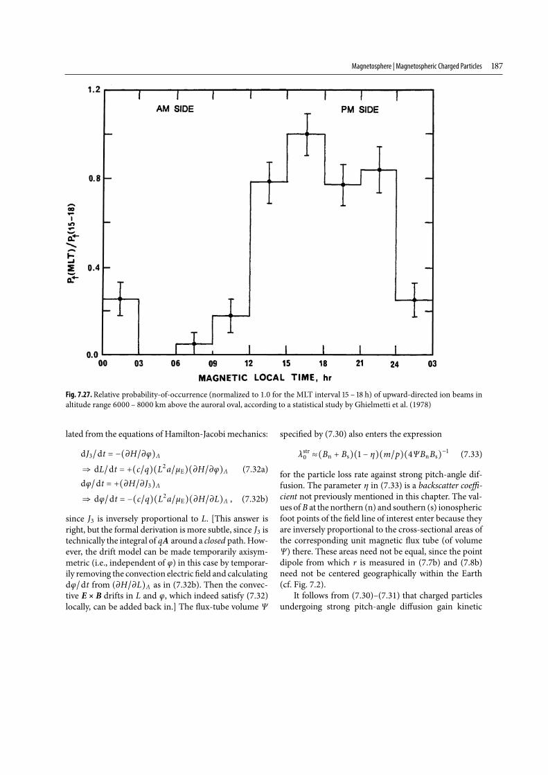
Magnetosphere | Magnetospheric Charged Particles

Fig. 7.27.Relative probability-of-occurrence (normalized to 1.0 for the MLT interval – h) of upward-directed ion beams inaltitude range – km above the auroral oval, according to a statistical study by Ghielmetti et al. (1978)

lated from the equations of Hamilton-Jacobi mechanics:

dJ�dt = −(∂H�∂φ)Λ" dL�dt = +(c�q)(La�μE)(∂H�∂φ)Λ (7.32a)dφ�dt = +(∂H�∂J)Λ" dφ�dt = −(c�q)(La�μE)(∂H�∂L)Λ , (7.32b)

since J is inversely proportional to L. [This answer isright, but the formal derivation ismore subtle, since J istechnically the integral of qA around a closed path.How-ever, the drift model can be made temporarily axisym-metric (i.e., independent of φ) in this case by temporar-ily removing the convection electric field and calculatingdφ�dt from (∂H�∂L)Λ as in (7.32b). Then the convec-tive E � B drifts in L and φ, which indeed satisfy (7.32)locally, can be added back in.] The flux-tube volume Ψ

specified by (7.30) also enters the expression

λstr �(Bn + Bs)( − η)(m�p)(ΨBnBs)− (7.33)

for the particle loss rate against strong pitch-angle dif-fusion. The parameter η in (7.33) is a backscatter coeffi-cient not previously mentioned in this chapter. The val-ues of B at the northern (n) and southern (s) ionosphericfoot points of the field line of interest enter because theyare inversely proportional to the cross-sectional areas ofthe corresponding unit magnetic flux tube (of volumeΨ) there. These areas need not be equal, since the pointdipole from which r is measured in (7.7b) and (7.8b)need not be centered geographically within the Earth(cf. Fig. 7.2).

It follows from (7.30)–(7.31) that charged particlesundergoing strong pitch-angle diffusion gain kinetic

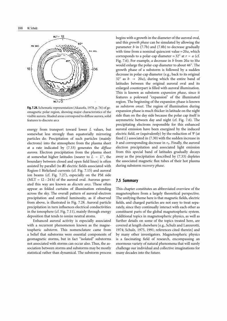
M. Schulz

Fig. 7.28.Schematic representation (Akasofu, 1978, p. 76) of ge-omagnetic polar region, showing major characteristics of thevisible aurora. Shaded areas correspond to diffuse aurora, solidfeatures to discrete arcs

energy from transport toward lower L values, butsomewhat less strongly than equatorially mirroringparticles do. Precipitation of such particles (mainlyelectrons) into the atmosphere from the plasma sheetat a rate indicated by (7.33) generates the diffuseaurora. Electron precipitation from the plasma sheetat somewhat higher latitudes (nearer to L = L�, theboundary between closed and open field lines) is oftenassisted by parallel (to B) electric fields associated withRegion-I Birkeland currents (cf. Fig. 7.15) and auroralion beams (cf. Fig. 7.27), especially on the PM side(MLT = – h) of the auroral oval. Auroras gener-ated this way are known as discrete arcs. These oftenappear as folded curtains of illumination extendingacross the sky. The overall pattern of auroral-electronprecipitation and emitted luminosity, as if observedfrom above, is illustrated in Fig. 7.28. Auroral particleprecipitation in turn influences electrical conductivitiesin the ionosphere (cf. Fig. 7.11), mainly through energydeposition that tends to ionize neutral atoms.

Enhanced auroral activity is especially associatedwith a recurrent phenomenon known as the magne-tospheric substorm. This nomenclature came froma belief that substorms were essential components ofgeomagnetic storms, but in fact “isolated” substormsnot associated with storms can occur also. Thus, the as-sociation between storms and substorms may be mostlystatistical rather than dynamical. The substorm process

begins with a growth in the diameter of the auroral oval,and this growth phase can be simulated by allowing theparameter b in (7.7b) and (7.8b) to decrease graduallywith time from a nominal quiescent value �a, whichcorresponds to a polar-cap diameter � � at r = a (cf.Fig. 7.6). For example, a decrease in b from a to awould enlarge the polar-cap diameter to about �. Thegrowth phase of a substorm is followed by a suddendecrease in polar-cap diameter (e.g., back to its original� as b � a), during which the entire band oflatitudes between the original auroral oval and itsenlarged counterpart is filled with auroral illumination.This is known as substorm expansion phase, since itfeatures a poleward “expansion” of the illuminatedregion. The beginning of the expansion phase is knownas substorm onset. The region of illumination duringexpansion phase is much thicker in latitude on the nightside than on the day side because the polar cap itself isasymmetric between day and night (cf. Fig. 7.6). Theprecipitating electrons responsible for this enhancedauroral emission have been energized by the inducedelectric field, or (equivalently) by the reduction of Ψ (atfixed L) associated in (7.30) with the sudden increase inb and corresponding decrease in r. Finally, the auroralelectron precipitation and associated light emissionfrom this special band of latitudes gradually decaysaway as the precipitation described by (7.33) depletesthe associated magnetic flux tubes of their hot plasmaduring substorm recovery phase.

7.5 Summary

This chapter constitutes an abbreviated overview of themagnetosphere from a largely theoretical perspective.The unifying theme here is that magnetic fields, electricfields, and charged particles are not easy to treat sepa-rately, since they continually interact with each other asconstituent parts of the global magnetospheric system.Additional topics in magnetospheric physics, as well asfurther details on some of the topics treated here, arecovered at length elsewhere [e.g., Schulz and Lanzerotti,1974; Schulz, 1975, 1991; references cited therein] andby many other investigators. Magnetospheric physicsis a fascinating field of research, encompassing anenormous variety of natural phenomena that will surelychallenge our individual and collective imaginations formany decades into the future.

Magnetosphere | References

Acknowledgement. The author thanks N. F. Ness for thenomination and Y. Kamide for the invitation to preparethis chapter. The author also thanks S. M. Petrinec, M.C.McNab,M. A. Rinaldi, andM.W.Chen for collabora-tions that generated Figs. ., .–., ., and .–.,respectively. This work was supported in part by NASAcontract NAS- for PIXIE data interpretation, inpart by NSF grant ATM- for Geospace Environ-ment Modeling (GEM), and in part by NSF grant ATM- for self-consistent ring-current modeling.

The author has benefited from reading colleagues’articles too numerous to cite in the subject-area of thischapter. However, this is not a review article, and the ref-erence list is admittedly unbalanced. The goal has beento provide access to further details and further sources ofinformation on topics treated here, or in some cases toacknowledge use of graphics first published elsewhere.In some instances the first report of a particular discov-ery has been left out in favor of a later but seeminglybetter treatment of the same topic.

References

Akasofu, S.-I. (1977) Physics of Magnetospheric Substorms,599 pp., Reidel, Dordrecht

Albert, J.M. (1994) Quasi-linear pitch angle diffusion coef-ficients: Retaining high harmonics, J. Geophys. Res., 99,23741–23745

Banks, P.M., and Holzer, T.E. (1969) High-latitude plasmatransport: The polar wind, J. Geophys. Res., 74, 6317–6332

Birmingham, T.J., and Jones, F.C. (1968) Identification ofmov-ing magnetic field lines, J. Geophys. Res., 73, 5505–5510

Brice, N.M. (1967) Bulk motion of the magnetosphere, J. Geo-phys. Res., 72, 5193–5211

Carpenter, D.L. (1966)Whistler studies of the plasmapause inthe magnetosphere: 1. Temporal variations in the positionof the knee and some evidence on plasma motions near theknee, J. Geophys. Res., 71, 693–709

Chen,M.W., Lyons, L.R., and Schulz,M. (1994) Simulations ofphase space distributions of stormtime proton ring currentprotons, J. Geophys. Res., 99, 5745–5759

Croley, D.R., Jr., Schulz, M., and Blake, J.B. (1976) Radial dif-fusion of inner-zone protons: Observations and variationalanalysis, J. Geophys. Res., 81, 585–594

Elkington, S.R., Hudson, M.K., and Chan, A.A. (1999) Accel-eration of relativistic electrons via drift-resonant interactionwith toroidal-mode Pc-5 ULF oscillations, Geophys. Res.Lett., 26, 3273–3276

Fälthammar, C.-G. (1968) Radial diffusion by violation ofthe third adiabatic invariant, in Earth’s Particles and Fields(edited by McCormac, B.M.), pp. 157–169, Reinhold, NewYork and London

Feldstein, Y.I. (1963) Some problems concerning themorphol-ogy of auroras and magnetic disturbances at high latitudes,Geomagn. i. Aeronom., 3, 227–239; English transl.: Geo-magn. Aeron., 3, 183–192

Ghielmetti, A.G., Johnson, R.G., Sharp, R.D., and Shelley, E.G.(1978) The latitudinal, diurnal, and altitudinal distributionsof upward flowing ions of ionospheric origin, Geophys. Res.Lett., 5, 59–62

Giraud, A., and Petit, M. (1978) Ionospheric Techniques andPhenomena, 264 pp., Reidel, Dordrecht

Gorney, D.J., and Evans, D.S. (1987) The low-latitude auro-ral boundary: Steady state and time-dependent representa-tions, J. Geophys. Res., 92, 13537–13545

Iijima, T., and Potemra, T.A. (1976) Field-aligned currents inthe dayside cusp observed by Triad, J. Geophys. Res., 81,5971–5979

Iijima, T., and Potemra, T.A. (1978) Large-scale characteristicsof field-aligned currents associated with substorms, J. Geo-phys. Res., 83, 599–615

Kivelson,M.G. (1976)Magnetospheric electric fields and theirvariation with geomagnetic activity, Rev. Geophys. SpacePhys., 14, 189–197

Lyons, L.R. (1973) Comments on pitch-angle diffusion in theradiation belts, J. Geophys. Res., 78, 6793–6797

Lyons, L.R., and Thorne, R.M. (1973) Equilibrium structure ofradiation belt electrons, J. Geophys. Res., 78, 2142–2149

Mayaud, P.N. (1980) Derivation, Meaning, and Use of Ge-omagnetic Indices, Geophys. Monogr. 22, Am. Geophys.Union, Washington, DC

Mead, G.D., and Beard, D.B. (1964) Shape of the geomagneticfield solar wind boundary, J. Geophys. Res., 69, 1169–1179

Nishida, A. (1966) Formation of a plasmapause, or magne-tospheric plasma knee, by combined action of magneto-spheric convection and plasma escape from the tail, J. Geo-phys. Res., 71, 5669–5679

Parker, E.N. (1963) Interplanetary Dynamical Processes, Wi-ley/Interscience, New York

Richmond, A.D., and Kamide, Y. (1988) Mapping of elec-trodynamic features of the high-latitude ionosphere fromlocalized observations: Techniques, J. Geophys. Res., 93,5741–5759

Schmidt, A. (1935) Tafeln der normierten Kugelfunktionen,sowie Formeln zur Entwicklung, Engelhard-Reyer, Gotha

Schulz, M. (1975) Geomagnetically trapped radiation, SpaceSci. Rev., 17, 481–536

Schulz, M. (1991) The magnetosphere, in Geomagnetism,vol. 4, edited by Jacobs, J.A., pp. 87–293, Academic Press,London and San Diego

M. Schulz

Schulz, M. (1998) Particle drift and loss rates under strongpitch-angle diffusion in Dungey’s model magnetosphere,J. Geophys. Res., 103, 61–67 and 15013

Schulz, M., and Eviatar, A. (1969) Diffusion of equatorialparticles in the outer radiation zone, J. Geophys. Res., 74,2182–2192

Schulz, M., and Koons, H.C. (1972) Thermalization of collid-ing ions streams beyond the plasmapause, J. Geophys. Res,77, 248–254

Schulz, M., and Lanzerotti, L.J. (1974) Particle Diffusion inthe Radiation Belts, 215 pp., Springer, Heidelberg

Schulz, M., and McNab, M.C. (1996) Source-surface mod-eling of planetary magnetospheres, J. Geophys. Res., 101,5095–5118

Sibeck, D.G., Lopez, R.E., and Roelof, E.C. (1991) Solar windcontrol of the magnetopause shape, location, and motion,J. Geophys. Res., 96, 5489–5495

Snyder, C.W., Neugebauer, M., and Rao, U.R. (1963) The solarwind velocity and its correlation with cosmic-ray variationsand with solar and geomagnetic activity, J. Geophys. Res.,68, 6361–6370

Speiser, T.W., and Lyons, L.R. (1984) Comparison of ananalytical approximation for particle motion in a currentsheet with precise numerical calculations, J. Geophys. Res.,89, 147–158

Spreiter, J.R., Summers, A.L., and Alksne, A.Y. (1966) Hydro-magnetic flow around the magnetosphere, Planet. SpaceSci., 14, 223–253

Stahara, S.S. (2002) Adventures in the magnetosheath: Twodecades of modeling and planetary applications of the

Spreiter magnetosheath model, Planet. Space Sci., 50,421–442

Stern, D. (1974) Models of the Earth’s electric field, Rept.X-602-74-159, NASA Goddard Space Flight Center,Greenbelt, MD

Stern, D.P. (1975) Quantitative models of magnetic andelectric fields in the magnetosphere, Rept. X-602-75-90,NASA Goddard Space Flight Center, Greenbelt, MD

Straus, J.M., and Schulz, M. (1976) Magnetospheric convec-tion and upper-atmospheric dynamics, J. Geophys. Res.,81, 5822–5832

Tsyganenko, N.A. (1995) Modeling the Earth’s magne-tospheric magnetic field confined within a realisticmagnetopause, J. Geophys. Res., 100, 5599–5612

Vette, J.I., Lucero, A.B., and Wright, J.A. (1966) Models ofthe Trapped Radiation Environment, Volume II: Inner andOuter Zone Electrons, NASA SP-3024, Washington, DC

Volland, H. (1973) A semi-empirical model of large-scalemagnetospheric electric fields, J. Geophys. Res., 78, 171–180

Volland, H. (1975) Models of global electric fields within themagnetosphere, Ann. Géophys., 31, 154–173

Weimer, D.R. (1995) Models of high-latitude electric poten-tials derived with a least error fit of spherical harmoniccoefficients, J. Geophys. Res., 100, 19595–19607

Weimer D.R. (2005) Improved ionospheric electrodynamicmodels and application to calculating Joule heating rates,J. Geophys. Res., 110, A05306, doi:10.1029/2004JA010884

Yasuhara, F., and Akasofu, S.-I. (1977) Field-aligned cur-rents and ionospheric electric fields, J. Geophys. Res., 82,1279–1284