Embed Size (px)
Citation preview

This electronic thesis or dissertation has been
downloaded from the King’s Research Portal at
https://kclpure.kcl.ac.uk/portal/
The copyright of this thesis rests with the author and no quotation from it or information derived from it
may be published without proper acknowledgement.
Take down policy
If you believe that this document breaches copyright please contact [email protected] providing
details, and we will remove access to the work immediately and investigate your claim.
END USER LICENCE AGREEMENT
This work is licensed under a Creative Commons Attribution-NonCommercial-NoDerivatives 4.0
International licence. https://creativecommons.org/licenses/by-nc-nd/4.0/
You are free to:
Share: to copy, distribute and transmit the work Under the following conditions:
Attribution: You must attribute the work in the manner specified by the author (but not in any way that suggests that they endorse you or your use of the work).
Non Commercial: You may not use this work for commercial purposes.
No Derivative Works - You may not alter, transform, or build upon this work.
Any of these conditions can be waived if you receive permission from the author. Your fair dealings and
other rights are in no way affected by the above.
Real-time Resource Management and Energy Trading for Green Cloud-RAN
Wan Ariffin, Wan Nur Suryani Firuz
Awarding institution:King's College London
Download date: 09. May. 2019
Real-time Resource Managementand Energy Trading for Green
Cloud-RANs
Wan Nur Suryani Firuz Bt Wan Ariffin
A thesis submitted in partial fulfillment
of the requirements for the degree of
Doctor of Philosophy
of
King’s College London.
Centre for Telecommunications Research
King’s College London
August 8, 2017

To my beloved husband, children, parents, mother in law and all family members.
Abstract
This thesis considers cloud radio access network (C-RAN), where the remote radio
heads (RRHs) are equipped with renewable energy resources and can trade energy
with the grid. Due to uneven distribution of mobile radio traffic and inherent inter-
mittent nature of renewable energy resources, the RRHs may need real-time energy
provisioning to meet the users demands. Given the amount of available energy
resources at RRHs, the main contributions of the thesis begin with introducing real-
time resource management strategies to the RRHs with a shortage of power budget
to select an optimal number of user terminals based on their available energy bud-
get. On the other hand, sparse beamforming strategies introduced in the second
part of the thesis account for all RRHs with or without a shortage of power and
take consideration of realistic constraints on fronthaul capacity restrictions. The
proposed strategies strike an optimum balance among the total power consumption
in the fronthaul through adjusting the degree of partial cooperation among RRHs,
RRHs total transmit power and the maximum or total spot-market energy cost. A
smart energy management strategy based on the combinatorial multi-armed bandit
(CMAB) theory for C-RAN, which is powered by a hybrid of grid and renewable
energy sources is studied in the last part of the thesis. A combinatorial upper confi-
dence bound (CUCB) algorithm to maximize the overall rewards, earned as a result
of minimizing the cost of energy trading at individual RRHs of the C-RAN has been
introduced. Adapting to the dynamic wireless channel conditions, the proposed
CUCB algorithm associates a set of optimal energy packages, to be purchased from
the day-ahead markets, to a set of RRHs to minimize the total cost of energy pur-
chase from the main power grid by dynamically forming super arms. A super arm is
Abstract 4
formed on the basis of calculating the instantaneous energy demands at the current
time slot, learning from the cooperative energy trading at the previous time slots
and adjusting the mean rewards of the individual arms.

Acknowledgements
First and foremost, I would like to thank my Lord who gave me the strength and the
means to embark upon the journey to my PhD.
This thesis would not have been possible without the guidance and the support
of several individuals who helped me along this most unforgettable experiences of
my life. I am sincerely grateful to my primal supervisor Dr. Mohammad Reza
Nakhai one of the most amazing personalities that I have come across in my life.
He provided a unique perspective on novel research directions and taught me to
maintain my integrity as a researcher. Indeed, he is an irreplaceable asset for King’s
College London.
My sincere gratitude is reserved for my thesis and VIVA voce examiners, As-
sociate Professor Dr. Soon Xin Ng (University of Southampton) and Professor
Muhammad Ali Imran (University of Glasgow) for their invaluable insights and
suggestions. I remain amazed that despite their busy schedules, they were able to
go through the final draft of my thesis within a few weeks with extremely useful
comments and suggestions.
Furthermore, I would like to express my appreciation to Professor Mischa
Dohler and Professor Hamid Aghvami (former), head of Centre of Telecomuni-
cation Research (CTR) department, for their vision, sagacity, and enthusiasm for
innovation. I am particularly grateful to my colleagues at CTR, including Sarah,
Sumayyah Dzulkifly, Hessa Alfraihi, Sunila Akbar, Nasreen Anjun, Halen, Hong,
and many others, who have convinced me that working hard is not incompati-
ble with having fun. Especially, I would like to acknowledge the efforts of my
best friends, Sumayyah Dzulkifly, Bibi Intan Suraya Murat, Nazahah Mustafa, Nur

Acknowledgements 6
Farhan Kahar, Nurfarah Athirah, and my team partner, Sarah, who are always by
my side during the tough times and helped me in improving the quality of this work.
Acknowledgments go to Universiti Malaysia Perlis (UniMAP) and Kemente-
rian Pengajian Tinggi (KPT), Malaysia for their financial and all the support. The
highest gratitude goes to the top managements of UniMAP and school of computer
and communication engineering (SCCE). Special dedications also go to my col-
leagues at SCCE, especially Shima, Aini, Aznor, Hasneeza, Rohani, Norma and
many others, who gave me hours of moral support and enjoyable time to finish my
thesis writing. I would like to acknowledge the efforts of Junita Nordin and Hasliza
A Rahim who helped me in improving the quality of this work by proofreading the
thesis.
Special thanks to all my family who always believed in me and encouraged me
to take on the most difficult of challenges in life. Thanks to my beloved husband,
Zahirul Fahmi Bin Zaini, who holds a special place in my heart and my children,
Nur Qalesya Humaira Binti Zahirul Fahmi, Nur Raudhah Mardhiah Binti Zahirul
Fahmi, Nur Hidayah Sofea Binti Zahirul Fahmi, Nur Inas Insyirah Binti Zahirul
Fahmi and Zahirul Iman Fathi Bin Zahirul Fahmi, the best gifts Allah has ever
given me. I am especially thankful to my loving parents, Wan Ariffin Bin Wan
Derahman and Fatimah Binti Mat Zin, my mother in law, Zainun Binti Rahim, my
siblings, Wan Noorul Hafilah, Wan Mohammad Najdan, Wan Shafini, Wan Mo-
hammad Hakiman, Wan Mohammad Alimin, Wan Mohammad Ariff, Wan Abdul
Qahhar, Wan Nur Syuhada, Wan Abdul Azim, and all my family members for their
selfless and boundless love all through the years. Their perpetual support is always
there no matter how far I travel away from home, since the hearts of our family are
intrinsically bound together. I dedicate this work to all my loves.
Contents
List of Figures 11
List of Tables 13
List of Algorithms 14
List of Abbreviations 15
List of Symbols 18
1 Introduction 22
1.1 Thesis Statement . . . . . . . . . . . . . . . . . . . . . . . . . . . 22
1.2 Thesis Motivation . . . . . . . . . . . . . . . . . . . . . . . . . . . 23
1.3 Thesis Contributions . . . . . . . . . . . . . . . . . . . . . . . . . 26
1.3.1 Contributions . . . . . . . . . . . . . . . . . . . . . . . . . 26
1.3.2 List of Publications . . . . . . . . . . . . . . . . . . . . . . 28
1.4 Thesis Outline . . . . . . . . . . . . . . . . . . . . . . . . . . . . . 29
2 Background Study 31
2.1 Introduction . . . . . . . . . . . . . . . . . . . . . . . . . . . . . . 31
2.2 Evolution of Cellular System . . . . . . . . . . . . . . . . . . . . . 31
2.3 Green Cloud Radio Access Networks : A Recent Trend for CoMP . 33
2.3.1 Renewable Energy Technologies for Green C-RANs . . . . 33
2.3.2 System Architecture of C-RANs with Renewable Energy
Technologies . . . . . . . . . . . . . . . . . . . . . . . . . 34
Contents 8
2.3.3 System Structures of Green C-RANs . . . . . . . . . . . . 37
2.4 Downlink Beamforming Design for Green C-RANs. . . . . . . . . 39
2.4.1 Beamforming . . . . . . . . . . . . . . . . . . . . . . . . . 39
2.4.2 Linear Antenna Array . . . . . . . . . . . . . . . . . . . . 41
2.4.3 Downlink Beamforming Design for Full Cooperation Mul-
tiuser C-RANs . . . . . . . . . . . . . . . . . . . . . . . . 45
2.5 Convex Optimization . . . . . . . . . . . . . . . . . . . . . . . . . 48
2.6 Semidefinite Programming (SDP) . . . . . . . . . . . . . . . . . . 52
2.7 Sparse Beamforming Design for C-RAN with SWIPT Systems . . . 55
2.8 Resource Management and Energy Trading with the Smart Grid . . 59
2.9 Related Works . . . . . . . . . . . . . . . . . . . . . . . . . . . . . 62
2.10 Concluding Remarks . . . . . . . . . . . . . . . . . . . . . . . . . 64
3 Real-Time Energy Management in Green C-RAN 65
3.1 Introduction . . . . . . . . . . . . . . . . . . . . . . . . . . . . . . 65
3.1.1 Organization . . . . . . . . . . . . . . . . . . . . . . . . . 66
3.2 System Model . . . . . . . . . . . . . . . . . . . . . . . . . . . . . 66
3.2.1 Energy Management Model . . . . . . . . . . . . . . . . . 66
3.2.2 Downlink Transmission Model . . . . . . . . . . . . . . . . 67
3.3 Strategy 1 : Power-Shortage Management by Partial Cooperation . . 69
3.3.1 Problem Formulation . . . . . . . . . . . . . . . . . . . . . 69
3.3.2 Convex Relaxation . . . . . . . . . . . . . . . . . . . . . . 71
3.4 Strategy 2 : Power-Shortage Management by Full Cooperation . . . 73
3.4.1 Problem Formulation . . . . . . . . . . . . . . . . . . . . . 73
3.4.2 Convex Relaxation . . . . . . . . . . . . . . . . . . . . . . 75
3.5 Strategy 3 : Overall Network Energy Management by Full Cooper-
ation . . . . . . . . . . . . . . . . . . . . . . . . . . . . . . . . . . 76
3.5.1 Problem Formulation . . . . . . . . . . . . . . . . . . . . . 76
3.5.2 Convex Relaxation . . . . . . . . . . . . . . . . . . . . . . 78
3.6 Simulation Results . . . . . . . . . . . . . . . . . . . . . . . . . . 78
3.7 Concluding Remarks . . . . . . . . . . . . . . . . . . . . . . . . . 83
Contents 9
4 Real-Time Energy Management in Fronthaul Constrained Green C-
RAN 84
4.1 Introduction . . . . . . . . . . . . . . . . . . . . . . . . . . . . . . 84
4.1.1 Organization . . . . . . . . . . . . . . . . . . . . . . . . . 87
4.2 System Model . . . . . . . . . . . . . . . . . . . . . . . . . . . . . 87
4.2.1 Downlink Transmission Model . . . . . . . . . . . . . . . . 88
4.2.2 An Iterative ET Authorization Algorithm . . . . . . . . . . 89
4.3 Strategy 1 : DRRHC with Min-Max Real-time Energy Purchase . . 90
4.3.1 Problem Formulation . . . . . . . . . . . . . . . . . . . . . 90
4.3.2 Resource Management Algorithm Design . . . . . . . . . . 92
4.4 Strategy 2 : DRRHC with Overall Energy Purchase Minimization . 95
4.4.1 Problem Formulation . . . . . . . . . . . . . . . . . . . . . 95
4.4.2 Resource Management Algorithm Design . . . . . . . . . . 95
4.5 Simulation Results . . . . . . . . . . . . . . . . . . . . . . . . . . 96
4.6 Concluding Remarks . . . . . . . . . . . . . . . . . . . . . . . . . 104
5 Combinatorial Multi-Armed Bandit Approach for Proactive Energy
Management in Green C-RAN 105
5.1 Introduction . . . . . . . . . . . . . . . . . . . . . . . . . . . . . . 105
5.1.1 Organization . . . . . . . . . . . . . . . . . . . . . . . . . 105
5.2 DRRHC with Overall Energy Purchase Minimization . . . . . . . . 106
5.3 Combinatorial Multi-Armed Bandit for Real-Time Energy Trading . 108
5.4 Strategy 1 : Forward Combinatorial Multi-Armed Bandit . . . . . . 110
5.5 Strategy 2 : Reverse Combinatorial Multi-Armed Bandit . . . . . . 113
5.6 Simulation Results . . . . . . . . . . . . . . . . . . . . . . . . . . 116
5.7 Concluding Remarks . . . . . . . . . . . . . . . . . . . . . . . . . 121
6 An Online Learning Approach : A Smart Energy Management 123
6.1 Introduction . . . . . . . . . . . . . . . . . . . . . . . . . . . . . . 123
6.1.1 Organization . . . . . . . . . . . . . . . . . . . . . . . . . 124
6.2 An Online Learning Approach for A Smart Real-Time Energy Trading124
Contents 10
6.2.1 Problem Formulation for Online Learning Approach . . . . 124
6.2.2 CUCB-CMAB Algorithms for Online Learning Approach . 126
6.3 Simulation Results . . . . . . . . . . . . . . . . . . . . . . . . . . 129
6.4 Concluding Remarks . . . . . . . . . . . . . . . . . . . . . . . . . 134
7 Conclusions and Future Research 135
7.1 Thesis Summary . . . . . . . . . . . . . . . . . . . . . . . . . . . 135
7.2 Avenues of Future Research . . . . . . . . . . . . . . . . . . . . . 139
7.2.1 Self Energy Storage . . . . . . . . . . . . . . . . . . . . . 139
7.2.2 Neighbourhood Energy Sharing and Trading . . . . . . . . 139
7.2.3 Game Theoretical Approach . . . . . . . . . . . . . . . . . 140
7.2.4 Robust Sparse Beamforming . . . . . . . . . . . . . . . . . 140
7.2.5 Multiple Input Multiple Output (MIMO) . . . . . . . . . . 140
Appendices 142
A Proof of Lemma 1 142
References 146
List of Figures
2.1 Non-cooperative cellular radio access networks (RANs). . . . . . . 32
2.2 Joint processing for cooperative transmission in the coordinated
multipoint (CoMP) networks. . . . . . . . . . . . . . . . . . . . . . 32
2.3 System architecture of a C-RAN with green technologies. . . . . . . 35
2.4 System structures of a C-RAN [1] . . . . . . . . . . . . . . . . . . 37
2.5 Estimation of direction of arrival (DoA). . . . . . . . . . . . . . . . 40
2.6 Beamforming technique. . . . . . . . . . . . . . . . . . . . . . . . 42
2.7 A schematic of a wavefront impinging across an array of antenna. . 43
2.8 Downlink beamforming in a full cooperation multiuser C-RAN. . . 47
2.9 Example of a convex cone [68]. . . . . . . . . . . . . . . . . . . . 49
2.10 Example of a convex function [68]. . . . . . . . . . . . . . . . . . . 50
2.11 A SWIPT system with separate information and energy receiving
terminals. . . . . . . . . . . . . . . . . . . . . . . . . . . . . . . . 56
2.12 Two-way communication and energy cooperation with the smart
power grid. . . . . . . . . . . . . . . . . . . . . . . . . . . . . . . 60
3.1 Power-shortage management by partial cooperation in the green C-
RAN. . . . . . . . . . . . . . . . . . . . . . . . . . . . . . . . . . 69
3.2 Power-shortage management by full cooperation in the green C-RAN. 73
3.3 Comparison of total transmit power for different strategies . . . . . 81
3.4 Comparison of behaviour of transmit power from RRH2 to individ-
ual ITs for different strategies at target SINR of γ = 25 dB . . . . . 82
3.5 Comparison of total energy cost for different strategies . . . . . . . 82
List of Figures 12
4.1 RRH-centric Clustering embedded with ETs Authorization Algorithm 85
4.2 A Multi-user Downlink SWIPT C-RAN Simulation Topology. . . . 96
4.3 Total energy cost versus various target SINR for different strategies. 99
4.4 Total transmit power versus various target SINR for different strate-
gies. . . . . . . . . . . . . . . . . . . . . . . . . . . . . . . . . . . 100
4.5 Transmit power variation of RRHs using reweighted `1-norm
method proposed in Algorithm 3 for serving the 3rd IT at γ = 20dB. 101
4.6 Clustering behaviour of RRH 3 at γ = 20dB target SINR. . . . . . . 102
4.7 Optimal energy trading for proposed strategies at γ = 30dB. . . . . 103
5.1 Combinatorial MAB problem for the proposed resource manage-
ment and energy trading in green C-RAN. . . . . . . . . . . . . . . 109
5.2 Flow chart for ForCMAB Energy Trading. . . . . . . . . . . . . . . 112
5.3 Flow chart for RevCMAB Energy Trading. . . . . . . . . . . . . . . 115
5.4 A Multi-user Downlink SWIPT C-RAN Simulation Topology. . . . 117
5.5 Total energy cost versus number of trials at γ = 20dB. . . . . . . . . 120
5.6 Total energy cost versus various target SINR at T = 24. . . . . . . . 120
5.7 Average set of optimal sizes of the energy packages to be purchased
from the day-ahead market decided by the CP at T = 24 and γ = 20dB.121
6.1 Proposed CUCB-CMAB strategy for Energy trading in C-RAN. . . 126
6.2 Normalized total energy cost versus index of time slot. . . . . . . . 131
6.3 Normalized total energy cost within 30 time slots. . . . . . . . . . . 131
6.4 Selected super arms by the CUCB-CMAB strategy. . . . . . . . . . 132
6.5 Normalized accumulated reward/regret versus index of time slot at
at the initial of each exploitation stage. . . . . . . . . . . . . . . . . 133
List of Tables
3.1 Simulation parameters for Chapter 3. . . . . . . . . . . . . . . . . . 80
4.1 Simulation parameters for Chapter 4. . . . . . . . . . . . . . . . . . 98
5.1 Simulation parameters for Chapter 5. . . . . . . . . . . . . . . . . . 119
6.1 Simulation parameters for Chapter 6. . . . . . . . . . . . . . . . . . 130
List of Algorithms
1 Reweighted `1-norm method for ITs . . . . . . . . . . . . . . . . . 72
2 An iterative ET authorization algorithm . . . . . . . . . . . . . . . 90
3 Reweighted `1-norm method for SWIPT . . . . . . . . . . . . . . . 93
4 Reweighted `1-norm method for SWIPT . . . . . . . . . . . . . . . 106
5 Forward CMAB (ForCMAB) Energy trading . . . . . . . . . . . . 113
6 Reverse CMAB (RevCMAB) Energy trading . . . . . . . . . . . . . 116
7 CMAB for Super Arm Exploration Algorithm. . . . . . . . . . . . . 127
8 CUCB-CMAB Main Algorithm . . . . . . . . . . . . . . . . . . . . 128

List of Abbreviations
AAS adaptive antenna system
AoA angle of arrival
AoD angle of departure
AP arithmetic progression
BBU baseband processing unit
BS base station
CAPEX capital expenditure
CDMA code-division multiple access
CMAB combinatorial multi-armed bandit
CO2 carbon dioxide
CoMP coordinated multipoint
CP centralized cloud computing processor
CPRI common public radio interface
C-RAN cloud radio access network
CSI channel state information
CUCB combinatorial upper confidence bound
DoA direction of arrival
DoD direction of departure
DRRHC Dynamic RRH-centric Clustering
e.g. for example
ET energy receiving terminal
ForCMAB forward combinatorial multi-armed bandit
GSMA Global Systems for Mobile communications Association
List of Abbreviations 16
ICI inter-cell interference
i.i.d. independent and identically distributed
i.e. that is
IT information receiving terminal
KKT Karush-Kuhn-Tucker
LHS left hand side
MAB multi-armed bandit
MAC medium access control
MBS master base station
MIMO multiple input multiple output
MISO multiple input single output
NP non-deterministic polynomial-time
OBSAI open base station architecture initiative
OFDM orthogonal frequency-division multiplexing
OFDMA orthogonal frequency-division multiple access
OPEX operating expense
PSD positive semidefinite
QoS quality of service
RAN radio access network
RevCMAB reverse combinatorial multi-armed bandit
RF radio frequency
RRH remote radio head
SAP successful access probability
SDP semidefinite programming
SDR semidefinite relaxation
SINR signal-to-interference-plus-noise ratio
SNR signal-to-noise ratio
SWIPT simultaneous wireless information and power transfer
ZMCSCG zero mean circularly symmetric complex Gaussian
1G first generation
List of Abbreviations 17
2G second generation
3G third generation
3GPP 3rd Generation Partnership Project
4G fourth generation
5G fifth generation

List of Symbols
w scalar w
w vector w
W matrix W
| w | magnitude of w
W∗ complex conjugate of W
WT transpose of W
WH complex conjugate transpose of W
tr(W) trace of W
vec(W) vectorization of matrix W which converts the matrix into an
column vector by stacking the columns of the matrix W on the
top of one another
rank(W) rank of W
minw
minimizes all the elements of w
s.t. subject to
[W]i, j the (i, j)th entry of W
E(·) expectation operator
W� 0 W is a positive semidefinite matrix
W� X W−X is a positive semidefinite matrix
w� 0 all elements of w are nonnegative
w� 0 all elements of w are positive
w� x element-wise greater than or equal to
w� x element-wise greater than
Cn sets of n dimensional complex vectors
List of Symbols 19
Rn sets of n dimensional real vectors
Cn×m sets of n-by-m dimensional complex matrices
Rn×m sets of n-by-m real matrices
CN(µ,Γ) circularly symmetric complex normal distribution with mean
µ and variance Γ
A ∈ B a set A is a subset of a set B which is all the elements of A are
contained in a set of B
x→ a x approaches a
‖.‖p `p-norm of a vector
‖.‖0 number of non-zero entries in the vector.
I identity matrix with a suitable sizemax∑
i=minwi summation of all the elements of wi where a set i is limits from
a minimum to a maximum values
∑i∈A
wi summation of all the elements of wi where a set i is a subset of
a set A
= equal to
∼ is similar to
≈ approximately equal to
6= not equal to
≥ greater than or equal to
≤ less than or equal to
� much less than
� much greater than
bx the base b and the exponent x, i.e., bx is the product of multiplying
x bases
ex the natural exponential function
logb(x) the logarithm of x to base b
O(log x) big oh (O ) is a notation to give an upper bound on a function log x
diag(x1, · · · ,xN) a diagonal matrix with the diagonal entries given by x1, · · · ,xN .
Also can be written as Bdiag(01 · · ·0i . . .In · · ·0N), where 0i is an

List of Symbols 20
M×M matrix with all-zero elements and In is an M×M identity matrix
Js−1 the normalized energy unit, i.e., Js−1, is adopted in this thesis
and thus the terms ’power’ and ’energy’ are mutually convertible.
List of Symbols for Energy Management Model
En the amount of renewable energy generated at the n-th RRH
B[ahead]n the amount of energy that has been purchased from the
day-ahead market for the n-th RRH
B[real]n the amount of energy that is necessary to be purchased from
the real-time market for the n-th RRH
Sn the amount of excessive energy sold back to the grid by
the n-th RRH
π [renew] the price of generating per unit renewable energy
π [ahead] the price of purchasing per unit energy from the day-ahead market
π [real] the price of purchasing per unit energy from the real-time market
π [sell] the price of selling back per unit energy to the grid
P[total]n the total energy consumption at the n-th RRH
P[Tx]n the total transmit power at the n-th RRH
P[circuit]n the non-transmission hardware circuit power consumption at the
n-th RRH
B[total] the total energy cost of all the RRHs in the green C-RAN
P[Tmax]n the maximum transmit power allowance at the n-th RRH
P[max]CP the maximum power provision at the CP
List of Symbols for Downlink Transmission Model
N the number of RRHs
M the number of antennas per RRH
Ke the number of active ETs
K[idle]e the number of idle ETs
Ki the number of ITs
List of Symbols 21
Lb = {1, · · · ,N} the set of indexes for the RRHs
Le = {1, · · · ,Ke} the set of indexes for the active ETs and L [idle]e = {1, · · · ,K[idle]
e }is the set of indexes for the idle ETs
Li = {1, · · · ,Ki} the set of indexes for the ITs.
Z = {1, · · · ,Z} the set of indexes for the RRHs that are in the shortage of power
where Z ⊂Lb
P[budget]z power budget at the z-th RRH
C[fronthaul]z the fronthaul capacity consumption for link between the CP and
the z-th RRH that is in power budget shortage
C[fronthaul]n fronthaul capacity consumption for link between the CP and
the n-th RRH
∑n∈Lb
{B[real]
n
}the overall real-time energy-purchase from the grid
maxn∈Lb
{B[real]
n
}the maximum real-time energy-purchase from the grid
∑z∈Z
P[Tx]z the total transmit power of the RRHs with shortage of power budget
P [coop] the number of total active cooperative links between the RRHs and
the receiving terminals
∑n∈Lb
P[Tx]n the total transmit power of all the RRHs
G [ET]e the total energy harvested by the e-th active ET
G [ET-idle]z the total amount of energy that can be harvested from surroundings
by the z-th idle ET
Chapter 1
Introduction
1.1 Thesis Statement
To meet the ever-increasing mobile data traffic and to provide pervasive always-
connected broadband packet services for next generation networks, base stations
(BSs) are proposed to be installed more densely to provide higher capacity [1, 2].
However, inter-cell interference (ICI) has become more severe and may lead to the
bottleneck of the network throughput. The operational costs of the network have
also increased due to energy consumption by the growing number of BSs.
Cloud radio access network (C-RAN) has been regarded as a promising so-
lution owing to its superiority in ICI mitigation, and reducing both the capital ex-
penditure (CAPEX) and the operating expense (OPEX) of the network operator [3].
In the proposed C-RAN architecture, the conventional BSs are physically detached
into two parts: baseband processing units (BBUs) that are grouped together as a
centralized cloud computing processor (CP) for designing all the coordination and
energy trading strategies, and the remaining remote radio heads (RRHs) that are
in charge of all radio frequency operations [4]. The data of information receiving
terminals (ITs) is available at the CP and will be delivered to the multiple collab-
orative RRHs via high-capacity low-latency fronthaul links such as optical fibre
links. However, due to a large number of densely deployed distributed RRHs, each
serving a time-varying number of receiving terminals in a highly dynamic wireless
environment, the amount of energy demand by the wireless network operator from
1.2. Thesis Motivation 23
the reliable source, i.e., grid will be highly variable and statistically unknown over
different times of the day. As a result, the network operator may need real-time
energy provisioning to meet all the receiving terminals’ demand, and may take a
risk of losing the profit.
C-RAN with a green energy technology has become a promising alternative
solution for powering next generation wireless networks. In this green C-RAN,
a large number of RRHs are installed with energy harvesting devices, i.e., solar
panels and wind turbines that are capable of harvesting energy from environmental
sources with a lower cost since renewable energy generation is generally cheaper
than electrical energy off the grid. However, the green energy supply is heavily
dependent on the weather and the installation site. Thus, it is impossible to fully
rely on the green sources for powering wireless networks.
With the advancing technologies in smart grid, each RRH with local renewable
energy generation allows the implementation of two-way energy trading with the
smart grid [5, 6]. In the case of insufficient renewable energy, an RRH can request
an amount of deficit energy from the grid to maintain its reliable operation and
alternatively can make a profit by selling an amount of excess energy to the smart
grid on an agreed price.
1.2 Thesis Motivation
Provided that all the RRHs are equipped with renewable energy harvesters and im-
plemented with two-way energy trading, [7] proposes a joint energy trading for full
cooperation scheme in coordinated multipoint (CoMP) network, where the data of
all the ITs is available at the CP and will be distributed to all RRHs for cooperative
transmission via fronthaul links. However, the data circulation between the CP and
the RRHs requires huge fronthaul signalling overhead when full coordination is en-
abled [8]. The design in [7] that takes no account of fronthaul capacity restrictions
may lead to infeasible results in a practical scenario.
Consequently, C-RAN with limited fronthaul capacity has been investigated by
the research community and sparse beamforming technique for partial cooperation
1.2. Thesis Motivation 24
is proposed to address the issue. With the implementation of sparse beamforming
technique in a downlink transmission, the CP then only needs to distribute the re-
ceiving terminal’s data to its serving RRHs. Motivated by the literature that sparse
beamforming technique is commonly formulated as a `1-norm optimization prob-
lem and handled with reweighted `1-norm method introduced in [9], [10–14] pro-
pose dynamic sparse beamforming designs subject to quality of service (QoS) con-
straints for capacity-limited fronthaul links in the C-RAN. The authors in [10] inte-
grate the aforementioned works with simultaneous wireless information and power
transfer (SWIPT) concept and study the resource allocation algorithm. However,
none of them take into account the renewable energy sources that can be further ex-
tended to a joint management of the resource allocation and energy trading for green
communication. For the next generation networks, it will be imperative to search
for energy-efficient and spectrum solutions to the resource allocation problems in
the C-RAN system powered by the smart grid and renewable energy generation.
This thesis addresses the questions of how to determine the best serving set of
RRHs and how to design the best network-wide beamformer for each of the receiv-
ing terminals, with the aims to minimize the total cost of the network operator and
to address all the given constraints. In general, these problems involve both uncer-
tainty and conflict of interest between the network operator and the RRHs, because
the network operator wish to minimize the total cost by serving as many receiving
terminals as possible, while from the RRHs’ perspective, serving more receiving
terminals consume more power and fronthaul capacity. Therefore, it becomes es-
sential to search for new mathematical solutions to find an optimal tradeoff between
the total transmit power, receiving terminal rates, and the fronthaul capacity.
The first core objective of this thesis is to study the potential of the sparse
beamforming technique in a joint cooperative resource management and energy
trading problem, to address the stated challenge. In Chapter 3 and Chapter 4, dif-
ferent sparse beamforming strategies are introduced in a joint cooperative resource
management and energy trading in green C-RAN, to scrutinize the advantages of
this partial cooperation scheme. Specifically, Chapter 4 integrates the C-RAN sys-
1.2. Thesis Motivation 25
tem with SWIPT concept and propose a joint energy trading and partial cooperation
design based on two sparse beamforming strategies to account for limited-capacity
fronthaul links in the green C-RAN. These strategies strike an optimum balance
among the total power consumption in the fronthaul through adjusting the degree of
partial cooperation among RRHs, RRHs total transmit power and the maximum or
total spot-market energy cost.
Motivated by an abstract idea of multi-armed bandit (MAB) problem, the sec-
ond core objective is to investigate and establish the potential of the MAB frame-
work in the proposed sparse beamforming design. The MAB is a class of sequential
optimization problems, where, at each trial, a player pulls an arm from a given J
arms in order to get an instantaneous reward [15]. Each of the arms is being asso-
ciated with independent and identically distributed (i.i.d.) stochastic rewards. The
problem investigated in this thesis is categorized as a combinatorial MAB (CMAB)
problem, where a super arm that consists of a set of N arms, N ⊂J is played and
the rewards of its relevant arms are observed individually in each trial [16]. In this
thesis, each arm corresponds to the size of an energy package to be purchased for
a RRH from the day-ahead market prior to the actual time of energy demand. At
each trial, a set of N RRHs may lose some rewards due to not selecting the best arm
instead of the played arms, called as regret. The objective of this CMAB problem
is to maximize the accumulated reward by observing the associated reward of new
arms, known as exploration, while simultaneously optimizing the decisions among
a set of arms based on existing knowledge, known as exploitation, in multiple tri-
als [17]. The work in Chapter 5 introduces two iterative energy trading algorithms
based on CMAB to search for a set of cost-efficient energy packages in ascending
and descending order of package sizes without accounting for the wireless channel
dynamic.
These solutions lead to the third core objective which is to develop an online
learning algorithm to manage the variability and uncertainty to maintain cost-aware
reliable operation in C-RAN. The proposed algorithm employs a CMAB model
and minimizes the energy cost over a long time horizon at RRHs. The algorithm
1.3. Thesis Contributions 26
preshedules a set of cost-efficient energy packages to be purchased from an ancillary
energy market for the future time slots by learning both from the cooperative energy
trading at previous time slots and exploring new energy scheduling strategies at the
current time slot. This work is presented in Chapter 6.
1.3 Thesis Contributions
1.3.1 Contributions
The major contributions of this thesis lead to the design of a smart online learning
system for real-time resource management and energy trading in green C-RANs
with the smart grid. Some key outcomes and findings of this work are summarized
below:
1. A joint cooperative resource management and two-way energy trading model
for C-RANs using the dynamic clustering technique is firstly proposed in
[18] and this technique is presented in Chapter 3. By controlling the number
of RRHs which jointly serve an IT within the coverage area, the clustering
technique can lessen the capacity requirements on the constrained-fronthaul
links. This chapter introduced three different cooperative real-time energy
trading strategies in C-RANs and applies a sparse beamforming technique to
find the optimal trade-off between the degree of partial cooperation among
the RRHs in serving the ITs and the total energy cost of the network operator.
2. Chapter 4 integrates a real-time energy trading strategy with SWIPT concept,
where the RRHs simultaneously transfer information beams to ITs and en-
ergy beams to active energy receiving terminals (ETs). Since energy could
be highly attenuated over a long distance propagation and in order to main-
tain the efficiency of SWIPT, an iterative authorization algorithm that allows
only those ETs situated close enough to the RRHs to receive wireless en-
ergy is introduced. On the top of that, two sparse optimization problems have
been formulated with more realistic scenarios where RRHs are constrained
with limited fronthaul capacities. This work has been published in [19]. The
1.3. Thesis Contributions 27
works that have integrated some other real-time energy trading strategies with
SWIPT concept are published in [20] and [21].
Initially, Chapter 3 and Chapter 4 assume a set of fixed sizes of energy pack-
ages has been purchased from the day-ahead market without the process of
monitoring the actual amount of energy consumption and energy generated at
the renewable energy harvesters at the individual RRHs.
3. Chapter 5 which is published in [22] further extends the works in previous
chapters to a learning-based practical approach modelled as a CMAB prob-
lem. The CP is assumed to has no initial knowledge of forthcoming power
budget and energy consumption at the individual RRHs. With various sizes
of energy packages which are offered in the day-ahead market, two algo-
rithms are developed, namely, ForCMAB Energy Trading and RevCMAB En-
ergy Trading, to determine a set of optimal sizes of the energy packages to
be purchased for the RRHs on the basis of actual energy supply and demand,
to further minimize the total energy cost of the network operator. The other
research related to MAB problem is published in [23].
4. Adapting to the dynamic wireless channel conditions, Chapter 6 which is pro-
posed in [24] develops a smart online learning system based on the CMAB
problem for the green C-RANs. A combinatorial upper confidence bound
(CUCB) algorithm is proposed to maximize the overall rewards, earned as
a result of minimizing the cost of energy trading at individual RRHs of the
C-RAN. The proposed CUCB algorithm associates a set of optimal energy
packages, to be purchased from the day-ahead markets, to a set of RRHs
to minimize the total cost of energy purchase from the main power grid by
dynamically forming super arms. A super arm is formed on the basis of cal-
culating the instantaneous energy demands at the current time slot, learning
from the cooperative energy trading at the previous time slots and adjusting
the mean rewards of the individual arms. The works in [25] and [26] have
applied this concept in different problems and scenarios.
1.3. Thesis Contributions 28
1.3.2 List of Publications
The publications that are related to the contributions of this thesis are listed as fol-
lows:
1. Wan Ariffin, W. N. S. F., Zhang, X., & Nakhai, M. R. (2015). Real-time
energy trading with grid in green cloud-RAN. In IEEE International Sym-
posium on Personal, Indoor, and Mobile Radio Communications (PIMRC).
IEEE.Vol. 2015-December, p. 748-752, 7343397 [18].
2. Wan Ariffin, W. N. S. F., Zhang, X., & Nakhai, M. R. (2016). Sparse Beam-
forming for Real-time Resource Management and Energy Trading in Green
C-RAN. IEEE Transactions on Smart Grid.10.1109/TSG.2016.2601718 [19].
3. Wan Ariffin, W. N. S. F., Zhang, X., & Nakhai, M. R. (2016). Sparse
Beamforming for Real-time Energy Trading in CoMP-SWIPT Networks. In
IEEE International Conference on Communications (IEEE ICC 2016). IEEE.
10.1109/ICC.2016.7510865 [20].
4. Wan Ariffin, W. N. S. F., Zhang, X., & Nakhai, M. R. (2015). Real-time
power balancing in green CoMP network with wireless information and en-
ergy transfer. In IEEE International Symposium on Personal, Indoor, and Mo-
bile Radio Communications (PIMRC). IEEE.Vol. 2015-December, p. 1574 -
1578, 7343549 [21].
5. Wan Ariffin, W. N. S. F., Zhang, X., & Nakhai, M. R. (2016). Combinato-
rial Multi-armed Bandit Algorithms for Real-time Energy Trading in Green
C-RAN. In IEEE International Conference on Communications (IEEE ICC
2016). IEEE. 10.1109/ICC.2016.7511448 [22].
6. Zhang, X., Nakhai, M. R., & Wan Ariffin, W. N. S. F. (2016). A Multi-
armed Bandit Approach to Distributed Robust Beamforming in Multicell Net-
works. In IEEE Global Communications Conference (GLOBECOM) . IEEE,
7841517. [23].
1.4. Thesis Outline 29
7. Wan Ariffin, W. N. S. F., Zhang, X., & Nakhai, M. R. (2017). Predictive
Energy Trading in C-RAN. Submitted to IEEE Transactions on Smart Grid.
[24].
8. Zhang, X., Nakhai, M. R., & Wan Ariffin, W. N. S. F. (2017). A Bandit
Approach to Price-Aware Energy Management in Cellular Networks. In IEEE
Communication Letters. DOI: 10.1109/LCOMM.2017.2687872. [25]
9. Zhang, X., Nakhai, M. R., & Wan Ariffin, W. N. S. F. (2017). Adaptive
Energy Storage Management in Green Wireless Networks. In IEEE Signal
Processing Letters. DOI: 10.1109/LSP.2017.2707059. [26]
1.4 Thesis OutlineThe rest of this thesis is organized as follows. A background study and literature
review of the works related to the proposed research topic are provided in Chapter
2. The aim of this chapter is to provide fundamental concepts and technical back-
ground studies that are required to understand the problem areas addressed in this
thesis. Subsequently, the main contributions of the thesis are discussed in Chapters
3, 4, 5 and 6. In Chapter 3, three different cooperative real-time energy trading
strategies in C-RANs are proposed to jointly minimize the energy consumption and
the real-time energy trading, under the constraints of demand and supply power bal-
ancing at RRHs and quality of service satisfaction at user terminals. These strate-
gies mainly focus on power-shortage management. Then, Chapter 4 integrates the
C-RANs system with SWIPT by introducing an iterative authorization algorithm.
In this chapter, two sparse optimization problems have been formulated with more
realistic scenarios where RRHs are constrained with limited fronthaul capacities.
Interestingly, Chapter 5 focus on the development of a learning-based practical ap-
proach modelled as the CMAB problem. With the aim to further reduce the total
energy cost of the network operator, the new responsibility of the CP is to determine
the set of optimal sizes of the energy packages to be purchased for the RRHs on the
basis of actual energy supply and demand. On the top of that, Chapter 6 develops an
online learning algorithm as a pre-scheduling mechanism to manage the variability

1.4. Thesis Outline 30
and uncertainty to maintain cost-aware reliable operation in CRANs. Finally the
thesis is concluded and some interesting directions for future studies are pointed
out in Chapter 7.
Chapter 2
Background Study
2.1 IntroductionThis chapter comprehensively surveys recent advances in fronthaul-constrained
cloud radio access networks (C-RANs) with renewable energy technologies, par-
ticularly major issues related to the impact of constrained fronthaul on quality of
service (QoS) of receiving terminals, energy efficiency and spectral efficiency. Fur-
thermore, this chapter provides technical background studies that are required to
understand the problem area, especially semidefinite programming (SDP) and a lin-
ear antenna array used for beamforming which are addressed in the contribution
chapters. The concepts presented in this chapter are beneficial to the developments
of resource management and energy trading schemes between the C-RANs and the
smart grid that will be introduced in Chapters 3, 4, 5 and 6.
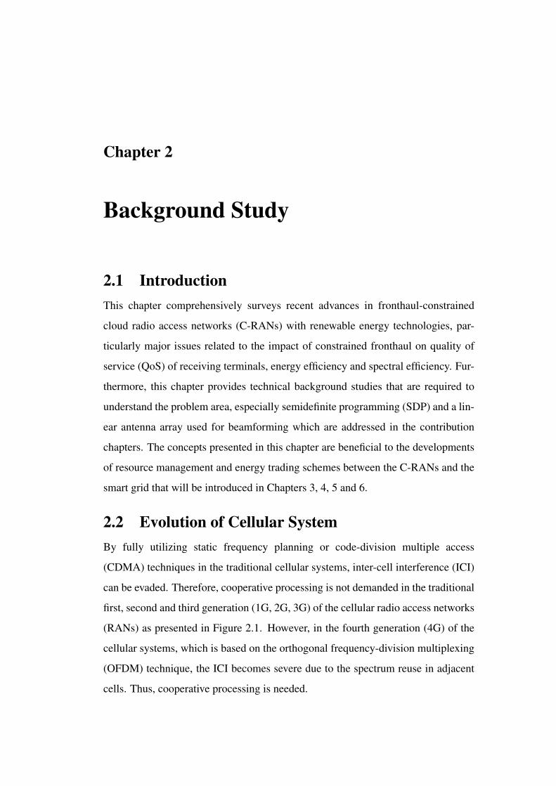
2.2 Evolution of Cellular SystemBy fully utilizing static frequency planning or code-division multiple access
(CDMA) techniques in the traditional cellular systems, inter-cell interference (ICI)
can be evaded. Therefore, cooperative processing is not demanded in the traditional
first, second and third generation (1G, 2G, 3G) of the cellular radio access networks
(RANs) as presented in Figure 2.1. However, in the fourth generation (4G) of the
cellular systems, which is based on the orthogonal frequency-division multiplexing
(OFDM) technique, the ICI becomes severe due to the spectrum reuse in adjacent
cells. Thus, cooperative processing is needed.
2.2. Evolution of Cellular System 32
Figure 2.1: Non-cooperative cellular radio access networks (RANs).
CoMP
CoMP
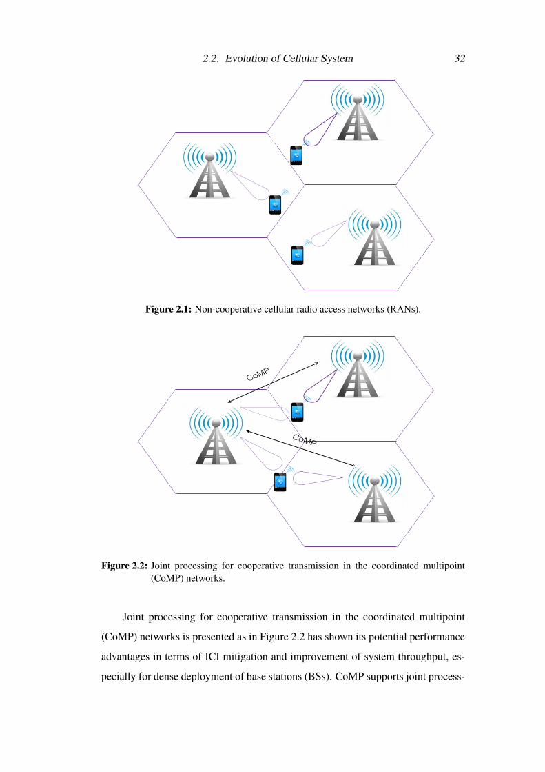
Figure 2.2: Joint processing for cooperative transmission in the coordinated multipoint(CoMP) networks.
Joint processing for cooperative transmission in the coordinated multipoint
(CoMP) networks is presented as in Figure 2.2 has shown its potential performance
advantages in terms of ICI mitigation and improvement of system throughput, es-
pecially for dense deployment of base stations (BSs). CoMP supports joint process-
2.3. Green Cloud Radio Access Networks : A Recent Trend for CoMP 33
ing for cooperative transmission, where the receiving terminal’s data is available at
multiple BSs, and the multiple BSs collaboratively serve every single receiving ter-
minal by simultaneously transmitting data towards it. Thus, the interference can be
exploited, and a significant performance gain can be achieved for full cooperation
in CoMP systems [12, 27].
2.3 Green Cloud Radio Access Networks : A Recent
Trend for CoMPA recent emerging deployment trend for CoMP network is to physically detach the
baseband processing units (BBUs) from conventional BSs and group them into a
BBU pool, i.e., a centralized cloud computing processor (CP). The remaining radio
units, i.e., remote radio heads (RRHs) with antennas located at the remote sites, are
connected to the BBUs via high-capacity low-latency fronthaul links, e.g., optical
fibre links. This promising network architecture known as C-RAN reduces both the
capital expenditure (CAPEX), i.e., the cost of developing non-consumable parts for
the C-RAN system, and the operating expense (OPEX), i.e., the ongoing cost for
running the C-RAN system, of the network operator [28].
2.3.1 Renewable Energy Technologies for Green C-RANs
A study shows that the cellular networks consumed world-wide is approximately
60 billion kWh per year [29]. In fact, the BSs consumed 80% of the electric-
ity in cellular networks. As a result, more than a hundred million tons of carbon
dioxide (CO2) per year has been produced and this figure is expected to double by
the year 2020 [1, 29]. Aware of this important huge energy consumption problem,
some methods for green communication has been studied in [30–33], particularly
for maximizing the energy efficiency of wireless communication systems.
A method for maximizing the energy efficiency using closed-form power allo-
cation technique is studied in [30]. With a minimum average throughput require-
ment, this method is proposed to be implemented for a point-to-point single carrier
system. Meanwhile, the studies in [31–33] focus on energy efficiency in cellular

2.3. Green Cloud Radio Access Networks : A Recent Trend for CoMP 34
multi-carrier multi-user systems for both uplink and downlink communications and
they proved the existence of a unique global maximum for the energy efficiency
for different systems. On contrary, the studies in [34–36] designed the system by
using multiple antennas to further maximize the energy efficiency. Power load-
ing algorithms with collocated and distributed antennas techniques have been pro-
posed in [34] and [35], respectively. Furthermore, [36] studies the effect of using a
large number of transmit antennas in orthogonal frequency-division multiple access
(OFDMA) systems.
With enormously increasing demand for mobile data and high data rates such
as online high definition video streaming and video conferencing, the aggregated
power requirements by user terminals may exceed the amount of power budget at
each of the RRHs in the C-RAN systems. Hence, the mobile network operators
may take a risk of losing the profit. One of the potential solutions to address this
issue and maintain the green communication is by using local renewable energy
generation [37–39]. It has been investigated that energy harvesting devices installed
at the RRHs can harvest energy from natural renewable energy sources such as
solar and wind. Therefore, C-RANs with renewable energy technologies can be
self-sustained and energy-efficient in providing ubiquitous service coverage.
2.3.2 System Architecture of C-RANs with Renewable Energy
Technologies
Equipping the RRHs with energy harvesting devices that can generate local renew-
able energy from environmental sources, e.g., solar and wind, green communica-
tions and energy trading have been considered as promising techniques to benefit
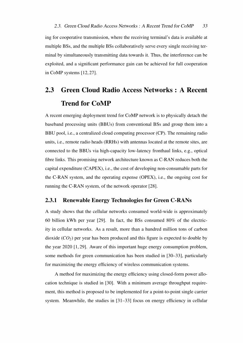
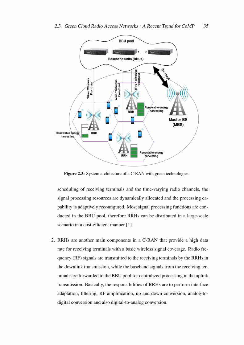
both the environment and the network operators. As shown in Figure 2.3, the gen-
eral architecture of a C-RAN with green technologies consists of four main compo-
nents as follows
1. In a C-RAN system, the BBUs clustered as a BBU pool is placed at a cen-
tralized site. The BBUs operate as virtual BSs to process baseband signals
as well as to optimize the radio resource allocation. Based on traffic-aware
2.3. Green Cloud Radio Access Networks : A Recent Trend for CoMP 35
Renewable energy harvesting
BBU pool
Baseband units (BBUs)
Wir
e / W
irel
ess
Fron
thau
l
Master BS(MBS)
Backhaul
RRH
RRH
RRH
Wir
e / W
irel
ess
Fron
thau
l
Wir
e / W
irel
ess
Fron
thau
l
Renewable energy harvesting
Renewable energy harvesting
Figure 2.3: System architecture of a C-RAN with green technologies.
scheduling of receiving terminals and the time-varying radio channels, the
signal processing resources are dynamically allocated and the processing ca-
pability is adaptively reconfigured. Most signal processing functions are con-
ducted in the BBU pool, therefore RRHs can be distributed in a large-scale
scenario in a cost-efficient manner [1].
2. RRHs are another main components in a C-RAN that provide a high data
rate for receiving terminals with a basic wireless signal coverage. Radio fre-
quency (RF) signals are transmitted to the receiving terminals by the RRHs in
the downlink transmission, while the baseband signals from the receiving ter-
minals are forwarded to the BBU pool for centralized processing in the uplink
transmission. Basically, the responsibilities of RRHs are to perform interface
adaptation, filtering, RF amplification, up and down conversion, analog-to-
digital conversion and also digital-to-analog conversion.
2.3. Green Cloud Radio Access Networks : A Recent Trend for CoMP 36
3. The link that connects the BBU pool and the RRH is known as fronthaul.
The link can be in a form of wire or wireless connection and its typical pro-
tocols include the common public radio interface (CPRI) and the open base
station architecture initiative (OBSAI) [40]. Ideal fronthaul without any con-
straints and non-ideal fronthaul with constraints are two types of fronthaul
links in the C-RAN architecture [1]. It has been written in [41] that the tra-
ditional coaxial-based systems on cell towers or legacy cell towers are being
completely overhauled and replaced by fiber for more capacity, longer-reach
distance and cost efficiency. The ideal fronthaul for C-RANs is optical fiber
communication without constraints because it can provide a high transmis-
sion capacity at the expense of high cost and difficult to deploy. On contrary,
wireless fronthauls are cheaper and more flexible to deploy, at the expense
of limited capacity and other constraints. Since the cost of wireless fronthaul
or capacity-constrained optical fiber is cheaper than the ideal optical fiber,
these technologies are anticipated to be prominent in practical C-RANs. In
addition, these technologies are flexible to set up. This thesis focuses only on
non-ideal capacity constrained fronthaul.
4. Powering radio RRH sites with renewable energy sources can reduce energy
costs significantly and improve the energy efficiency. In fact, the renewable
energy resources do not generate greenhouse gases such as carbon footprint
or CO2 because renewable energy is derived from resources that are regen-
erative. 25 leading telecoms including MTN Uganda and Zain, united under
the Global Systems for Mobile communications Association (GSMA) started
a program named ”Green Power for Mobile” [42, 43]. The main objective
of this program is to use renewable energy resources such as solar, wind or
sustainable biofuels technologies to power new and existing off-grid BSs and
BSs that are in bad-grid locations. By 2020, estimates indicate that the global
telecom industry will deploy approximately 390,000 BSs that are off-grid,
and 790,000 BSs that are in bad-grid locations [44]. By implementing this
renewable energy technologies, approximately 150 million barrels of diesel

2.3. Green Cloud Radio Access Networks : A Recent Trend for CoMP 37
per annum can be saved and annual carbon emissions can be reduced up to 45
million tonnes [44].
2.3.3 System Structures of Green C-RANs
As illustrated in Figure 2.4, system structures of C-RAN can be classified into three
main options depending on the fronthaul constraints and the different function split-
ting between BBUs and RRHs. The three main options are full centralization struc-
ture, partial centralization structure and hybrid centralization structure.
Figure 2.4: System structures of a C-RAN [1]
The premier C-RAN configuration is a full centralization structure. This struc-
ture known as the stacked BBU structure has significant benefits in terms of opera-
tion and maintenance, but incurs a high burden on fronthaul since the functions of
the physical layer, the medium access control (MAC) layer and the network layer,
i.e., Layer 1, Layer 2, Layer 3, of the conventional BS are moved into the BBU [45].
As a result, the BBU contains all processing and managing functions of the tradi-
tional BS and the performance of the C-RAN is clearly constrained by the fronthaul
2.3. Green Cloud Radio Access Networks : A Recent Trend for CoMP 38
link capacity. With densely deployed RRHs, the fronthaul traffic generated from a
receiving terminal with several MHz bandwidth could be easily scaled up to multi-
ple Gb/s. This is because, each of the transmitted RF signals by a receiving terminal
need to be sampled and quantized at the RRHs and then forwarded to the BBU pool.
Even under moderate mobile traffic, a commercial fiber link with tens of GHz ca-
pacity could thus be easily overwhelmed.
The second option is a partial centralization structure. This structure is also
called as stand-alone Layer 1 structure, where the RRH integrates the RF functions
and some strictly RF-related baseband processing functions. The other functions
in the physical layer and the upper layers remain in the BBU. The advantages of
this structure are the RRH-BBU overhead and the constraints on fronthaul can be
alleviated since the major computational burden of RANs is in the physical layer.
However, the disadvantages of this structure are some advanced features such as
CoMP transmission and reception, and spatial cooperative processing for distributed
massive multiple input multiple output (MIMO) cannot be supported efficiently. In
addition, the interaction and connection between physical layer and MAC layer
could also be complex and more difficult.
Hybrid centralization is the other option for the C-RAN structure. The partial
functions in physical layer such as the user specific or cell specific signal processing
functions are removed from BBUs and assembled into a new separated processing
unit, which may be a part of the BBU pool. The advantage of the hybrid central-
ization is its flexibility to support resource sharing and low energy consumption in
BBUs.
In this thesis, several advance strategies based on sparse beamforming tech-
nique to optimize the performance under a fully centralized structure are proposed
as it simplifies the functions and capabilities of the RRHs. For future research, these
works can be extended to decentralized structure for huge network cooperation. A
good cooperation mechanism design is required to motivate all the C-RANs in a
huge decentralized network structure to support the inter-system joint cooperation.
2.4. Downlink Beamforming Design for Green C-RANs. 39
2.4 Downlink Beamforming Design for Green C-
RANs.
2.4.1 Beamforming
In the beginning of a traditional cellular system, each BS has no information about
the locations of the receiving terminals in its serving area. Thus, the BS simply
radiates the dedicated information signals blindly in all directions within the sector
cell depending to its pattern. As a result, the dedicated information signals to the
intended receiving terminals would interfere to the other receiving terminals within
nearby cells, which are working on the same frequency as co-channel cells is im-
plemented. As its spread to areas with no present recipients, energies are wasted.
It is consider as an ideal scenario if the BS had perfect knowledge of the ex-
act locations of the receiving terminals. However this assumption is overly opti-
mistic, with no feasible hardware to make that precision and this configuration is
impossible in a practical scenario. Initially, the work that addresses array process-
ing of incoming signals has been reported in [46]. Then, more studies in the area
of beamforming has been done for space division purposes in mobile communica-
tions [47–60]. The authors in [47] were the first to develop an adaptive beamforming
technique.
Beamforming can create different radiation patterns by using antenna arrays
and an adaptive algorithm. The variable patterns created by beamforming technique
follow from spatial constructive and destructive interference of the signal wavefront
in different directions. A pattern changes when the signal feeding the different an-
tenna elements is phased. Generally, such procedure steers the main lobe in the
plane where the elements are arranged and eventually the nulls are steered as well.
By changing each element’s signal amplitude, a large variety of possible patterns
can be achieved [61]. A detailed knowledge about a receiving terminal location is
needed to develop a proper formation of the beams. Location detection techniques
using electronic scanning with antenna arrays have been developed mainly for mili-
tary purposes and satellite communications. Lately, this technique has been applied
2.4. Downlink Beamforming Design for Green C-RANs. 40
in cellular networks. Particularly, [62] reports in detail several location detection
techniques. The techniques to detect the locations of receiving terminals usually
coined as estimation of direction of arrival (DoA) or angle of arrival (AoA). The
idea is to find the angle between the receiving terminal-BS line and the antenna
boresight. Note that the antenna boresight is the plane perpendicular to the antenna
surface. To get the right position, the BS has to respond to the receiving terminal in
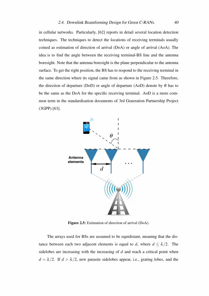
the same direction where its signal came from as shown in Figure 2.5. Therefore,
the direction of departure (DoD) or angle of departure (AoD) denote by θ has to
be the same as the DoA for the specific receiving terminal. AoD is a more com-
mon term in the standardisation documents of 3rd Generation Partnership Project
(3GPP) [63].
. . .Antenna!elements
θ
d
Figure 2.5: Estimation of direction of arrival (DoA).
The arrays used for BSs are assumed to be equidistant, meaning that the dis-
tance between each two adjacent elements is equal to d, where d ≤ λ/2. The
sidelobes are increasing with the increasing of d and reach a critical point when
d = λ/2. If d > λ/2, new parasite sidelobes appear, i.e., grating lobes, and the
2.4. Downlink Beamforming Design for Green C-RANs. 41
result of spatial undersampling of the transmitted signal or the received signal. This
phenomenon is an analogous to the aliasing effect that appears when this signal is
undersampled. Grating lobes lead to ambiguities in the directions of the depart-
ing or arriving signals. This is because parasite copies of these signals replicate
themselves in space in unwanted directions.
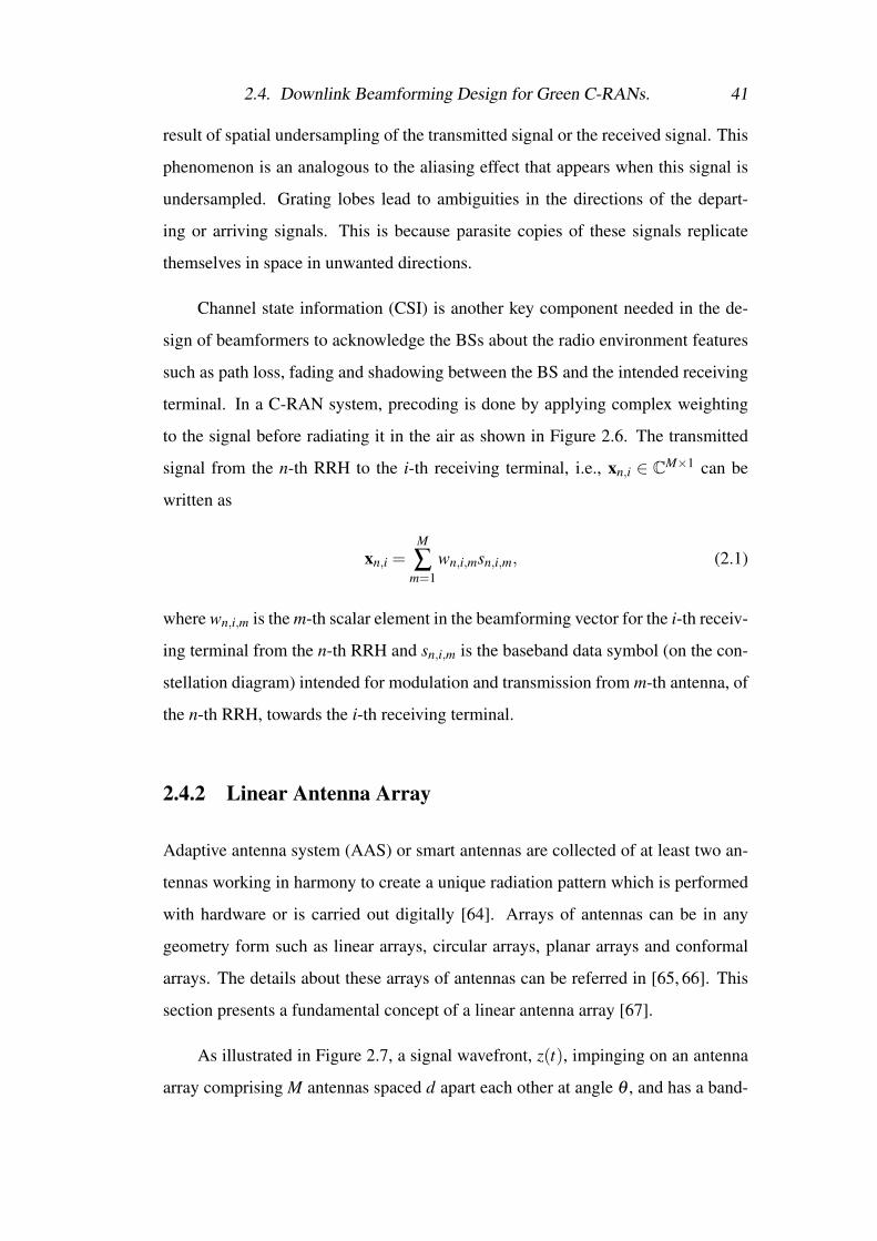
Channel state information (CSI) is another key component needed in the de-
sign of beamformers to acknowledge the BSs about the radio environment features
such as path loss, fading and shadowing between the BS and the intended receiving
terminal. In a C-RAN system, precoding is done by applying complex weighting
to the signal before radiating it in the air as shown in Figure 2.6. The transmitted
signal from the n-th RRH to the i-th receiving terminal, i.e., xn,i ∈ CM×1 can be
written as
xn,i =M
∑m=1
wn,i,msn,i,m, (2.1)
where wn,i,m is the m-th scalar element in the beamforming vector for the i-th receiv-
ing terminal from the n-th RRH and sn,i,m is the baseband data symbol (on the con-
stellation diagram) intended for modulation and transmission from m-th antenna, of
the n-th RRH, towards the i-th receiving terminal.
2.4.2 Linear Antenna Array
Adaptive antenna system (AAS) or smart antennas are collected of at least two an-
tennas working in harmony to create a unique radiation pattern which is performed
with hardware or is carried out digitally [64]. Arrays of antennas can be in any
geometry form such as linear arrays, circular arrays, planar arrays and conformal
arrays. The details about these arrays of antennas can be referred in [65, 66]. This
section presents a fundamental concept of a linear antenna array [67].
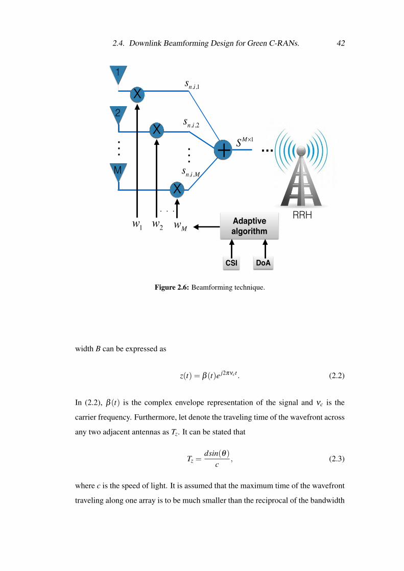
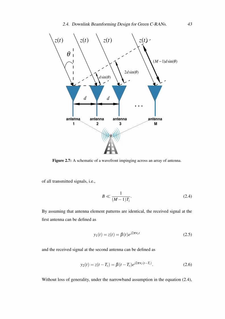
As illustrated in Figure 2.7, a signal wavefront, z(t), impinging on an antenna
array comprising M antennas spaced d apart each other at angle θ , and has a band-
2.4. Downlink Beamforming Design for Green C-RANs. 42
w1 w2 wM
. . .
xSM×1+. .
.
x
x
. . .
Adaptive!algorithm
CSI DoA
…
1
2
M
sn,i,1
RRH
sn,i,M
sn,i,2
. . .
Figure 2.6: Beamforming technique.
width B can be expressed as
z(t) = β (t)e j2πνct . (2.2)
In (2.2), β (t) is the complex envelope representation of the signal and νc is the
carrier frequency. Furthermore, let denote the traveling time of the wavefront across
any two adjacent antennas as Tz. It can be stated that
Tz =dsin(θ)
c, (2.3)
where c is the speed of light. It is assumed that the maximum time of the wavefront
traveling along one array is to be much smaller than the reciprocal of the bandwidth
2.4. Downlink Beamforming Design for Green C-RANs. 43
. . .
antenna! 1
θ
dd
z(t) z(t) z(t) z(t)
d sin(θ )
(M −1)d sin(θ )
2d sin(θ )
antenna! 2
antenna! 3
antenna! M
Figure 2.7: A schematic of a wavefront impinging across an array of antenna.
of all transmitted signals, i.e.,
B� 1(M−1)Tz
. (2.4)
By assuming that antenna element patterns are identical, the received signal at the
first antenna can be defined as
y1(t) = z(t) = β (t)e j2πνct (2.5)
and the received signal at the second antenna can be defined as
y2(t) = z(t−Tz) = β (t−Tz)e j2πνc(t−Tz). (2.6)
Without loss of generality, under the narrowband assumption in the equation (2.4),
2.4. Downlink Beamforming Design for Green C-RANs. 44
B� 1/Tz. It is clear that
β (t−Tz)≈ β (t). (2.7)
Let denote the wavelength of the signal wavefront as λc and νc/c = 1/λc, then the
received signal at the second antenna can be rewritten as follows
y2(t) = y1(t)e− j2πsin(θ) d
λc . (2.8)
Similarly, the received signal at the k-th antenna, i.e., k = 1,2, · · · ,M, can be calcu-
lated as
yk(t) = y1(t)e− j2π(k−1)sin(θ) d
λc . (2.9)
By referring to the equations (2.5), (2.8) and (2.9), it can be concluded that the
signals received at any two array elements are identical except for a phase shift
which depends on the angle of arrival and the array geometry.
Now, let consider a free field environment where neither scatterers and nor
multipath exists. A planar continuous-wave wavefront of frequency νc arriving
from an angle θ will introduce a spatial signature across the antenna array. This
spatial signature is a function of AoA, antenna element patterns and antenna array
geometry. The complex M×1 vector called as array response vector is
a(θ) =[
a1(θ) a2(θ) · · · aM(θ)]T
. (2.10)
Therefore, for the linear antenna array with identical element patterns, the array
response vector can be written as
a(θ) =
1
e− j2πsin(θ) dλc
...
e− j2π(M−1)sin(θ) dλc
. (2.11)
Similarly, the array response vector for a transmit linear antenna array with identical
2.4. Downlink Beamforming Design for Green C-RANs. 45
element patterns also can be translated as
a(θ) =[
1 e− j2πsin(θ) dλc · · · e− j2π(M−1)sin(θ) d
λc
]. (2.12)
As a result, the multiple input single output (MISO) channel between the antenna
array and a receiving terminal i can be defined as
hi = ξia(θi), (2.13)
where ξi captures both effects of channel fading, i.e., fast and slow fading, and
pathloss. Besides, θi is the AoD of the receiving terminal i with respect to the
broadside of the antenna array. Antenna arrays open up a spatial dimension to im-
prove capacities of wireless communication systems due to the fact that smart beam
patterns can be shaped by controlling the phases of individual antennas of the array.
Interestingly, power-efficient beams can be steered towards intended receiving ter-
minals. Therefore, the interference imposed on unintended receiving terminals can
be diminished. Smart beam patterns are performed via algorithms based on certain
criteria and can be implemented using hardware or software. However, the latter
technique is easier to operate such as using digital signal processing [64]. For in-
stance, these criteria could be either minimising transmit power with constraints on
receiving terminals’ signal-to-interference-plus-noise ratios (SINRs) or maximising
receiving terminals’ sum rate with constraints on transmit power.
2.4.3 Downlink Beamforming Design for Full Cooperation Mul-
tiuser C-RANs
Let consider a green C-RAN system that consists of a BBU pool, N RRHs, each
is equipped with M antennas and installed with a renewable energy harvesting de-
vice, and Ki single antenna information-receiving terminals (ITs). Furthermore, let
Lb = {1, · · · ,N} and Li = {1, · · · ,Ki}, respectively, indicate the set of indexes of
the RRHs and the ITs in the green C-RAN system. Let wni ∈ CM×1 be the beam-
forming vector formed by the n-th RRH towards the i-th receiving terminal, i ∈Li.
2.4. Downlink Beamforming Design for Green C-RANs. 46
We view all N RRHs of the C-RAN as a single virtual RRH and formulate the prob-
lem from the perspective of sparse optimisation. The antennas of the virtual RRH
can be partitioned into N groups, each corresponding to an individual RRH. Let
wi = [wH1i, · · · ,wH
Ni]H ∈ CMN×1 indicate the beamforming vector formed by the vir-
tual RRH towards the i-th receiving terminal. Let wn = [wHn1, · · · ,wH
nKi]H ∈ CMN×1
denote the beamforming vector formed by the n-th RRH towards the all of the Ki
receiving terminals in the C-RAN system. The requirement that some RRHs may
not participate in a transmission towards the i-th receiving terminal, due to some en-
ergy restrictions, translates to the group sparse structure of the virtual beamformer,
i.e., wi. That is, if wni = 0, then the n-th RRH is not participating in serving the i-th
receiving terminal. Similarly, inserting wni = 0 in wn means that the i-th receiving
terminal is not served by the n-th RRH, due to shortage of energy budget at the n-th
RRH.
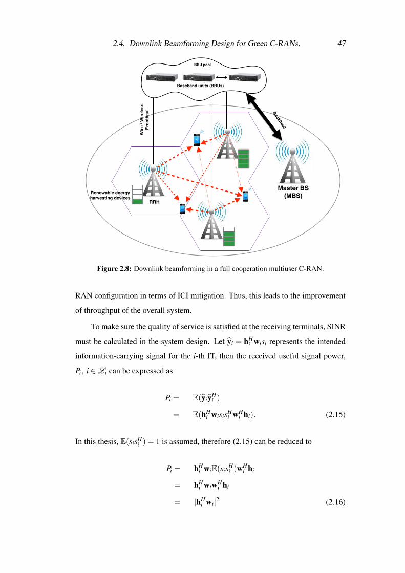
For a full cooperation system configuration, all the beamformers from the
RRHs in a C-RAN are participating in serving all the receiving terminals, as il-
lustrated in Figure 2.8. Mathematically, in this configuration, wni 6= 0, ∀n ∈ Lb,
∀i ∈Li.
Let hn,i ∈ CM×1 denote the channel vector between the n-th RRH and the i-th
receiving terminal. Then, the received signals at the i-th receiving terminal, i ∈Li
in a C-RAN downlink network, i.e., yi ∈ C can be expressed as
yi = hHi wisi + ∑
j=Li, j 6=ihH
i w js j +ni, (2.14)
where hi = [hH1i, · · · ,hH
Ni]H ∈ CMN×1 denotes the overall channel vector from the
virtual RRH to the i-th receiving terminal, si ∼ CN(0,1) is the intended symbol for
the i-th receiving terminal and ni ∼ CN(0,σ2i ) is the zero-mean circularly symmet-
ric complex Gaussian (ZMCSCG) noise. The terms at the right hand side of (2.14),
respectively, represent the intended information-carrying signal for the i-th IT, the
inter-user interference caused by all other non-desired information beams, and the
additive white Gaussian noise. Note that (2.14) confirms the advantage of the C-
2.4. Downlink Beamforming Design for Green C-RANs. 47
Renewable energy harvesting devices
BBU pool
Baseband units (BBUs)
Wire
/ W
irele
ssFr
onth
aul
Master BS(MBS)
Backhaul
RRH
Figure 2.8: Downlink beamforming in a full cooperation multiuser C-RAN.
RAN configuration in terms of ICI mitigation. Thus, this leads to the improvement
of throughput of the overall system.
To make sure the quality of service is satisfied at the receiving terminals, SINR
must be calculated in the system design. Let yi = hHi wisi represents the intended
information-carrying signal for the i-th IT, then the received useful signal power,
Pi, i ∈Li can be expressed as
Pi = E(yiyHi )
= E(hHi wisisH
i wHi hi). (2.15)
In this thesis, E(sisHi ) = 1 is assumed, therefore (2.15) can be reduced to
Pi = hHi wiE(sisH
i )wHi hi
= hHi wiwH
i hi
= |hHi wi|2 (2.16)
2.5. Convex Optimization 48
Let assume the noise variance, σ2i is identical at all receiving terminals. Then, the
SINR at the i-th IT, SINR[IT]i , i ∈Li, can be defined as
SINR[IT]i =
|hHi wi|2
∑j=Li, j 6=i
|hHi w j|2 +σ2
i. (2.17)
2.5 Convex Optimization
Convex optimization has become the most widely researched area in optimization
because of its ability in solving very large, practical engineering problems reliably
and efficiently. Optimization is a mathematical programming for selecting the best
possible element, satisfying the given constraints [68]. The objective of the op-
timization problem is to minimise or maximise a function. Convex optimization
deals with the minimisation of a convex objective function or maximisation of a
concave function subjected to convex constraints. Background study of convex op-
timisation are comprehensively discussed in [68–72] and can be perfectly applied to
either engineering field or non-engineering field like communications, signal pro-
cessing, mechanics, logistics, finance and many others [73].
In telecommunication, some problems can be translated into convex optimiza-
tion problems. If a problem is in a convex form, then it can provide a globally op-
timal solution. But most of telecommunication practical problems are non-convex
and the hardest part is to transform into a convex form. If the problem cannot be
transformed into a convex form, then a simplification procedure can be used and
would seek a sub-problem, convergent to a solution of the original problem.
A set C is convex if the line segment between any two points in C lies in C .
For instance, for any x1,x2 ∈ C and 0≤ θ ≤ 1, if
θx1 +(1−θ)x2 ∈ C , (2.18)
the set C is convex set. In the convex set C , every point in the set can be seen by
every other point, along an unobstructed straight path between them, where unob-
structed means lying in the set.
2.5. Convex Optimization 49
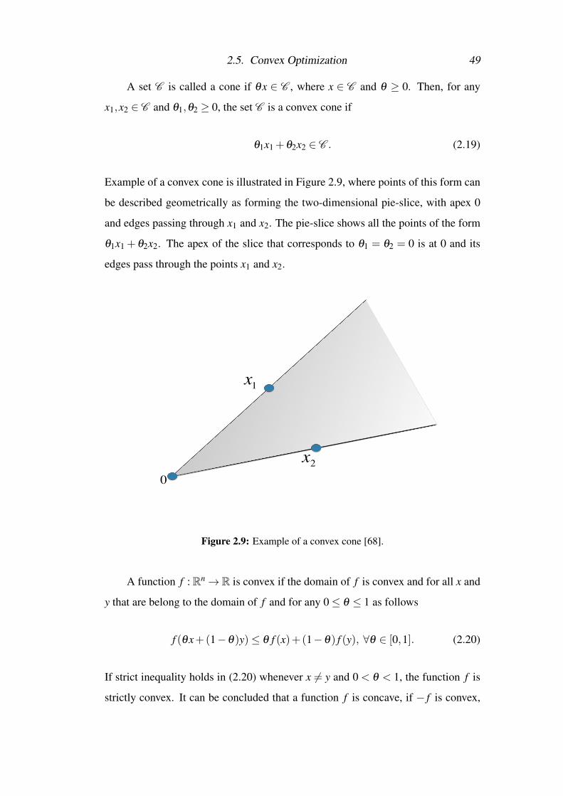
A set C is called a cone if θx ∈ C , where x ∈ C and θ ≥ 0. Then, for any
x1,x2 ∈ C and θ1,θ2 ≥ 0, the set C is a convex cone if
θ1x1 +θ2x2 ∈ C . (2.19)
Example of a convex cone is illustrated in Figure 2.9, where points of this form can
be described geometrically as forming the two-dimensional pie-slice, with apex 0
and edges passing through x1 and x2. The pie-slice shows all the points of the form
θ1x1 + θ2x2. The apex of the slice that corresponds to θ1 = θ2 = 0 is at 0 and its
edges pass through the points x1 and x2.
x1
x20
Figure 2.9: Example of a convex cone [68].
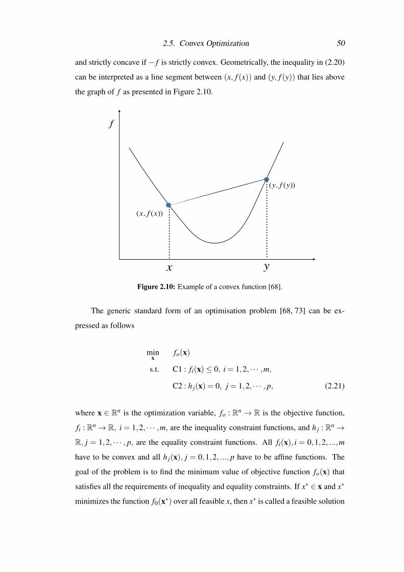
A function f : Rn→R is convex if the domain of f is convex and for all x and
y that are belong to the domain of f and for any 0≤ θ ≤ 1 as follows
f (θx+(1−θ)y)≤ θ f (x)+(1−θ) f (y), ∀θ ∈ [0,1]. (2.20)
If strict inequality holds in (2.20) whenever x 6= y and 0 < θ < 1, the function f is
strictly convex. It can be concluded that a function f is concave, if − f is convex,
2.5. Convex Optimization 50
and strictly concave if − f is strictly convex. Geometrically, the inequality in (2.20)
can be interpreted as a line segment between (x, f (x)) and (y, f (y)) that lies above
the graph of f as presented in Figure 2.10.
(x, f (x))
(y, f (y))
y
f
xFigure 2.10: Example of a convex function [68].
The generic standard form of an optimisation problem [68, 73] can be ex-
pressed as follows
minx
fo(x)
s.t. C1 : fi(x)≤ 0, i = 1,2, · · · ,m,
C2 : h j(x) = 0, j = 1,2, · · · , p, (2.21)
where x ∈ Rn is the optimization variable, fo : Rn → R is the objective function,
fi : Rn→ R, i = 1,2, · · · ,m, are the inequality constraint functions, and h j : Rn→R, j = 1,2, · · · , p, are the equality constraint functions. All fi(x), i = 0,1,2, ...,m
have to be convex and all h j(x), j = 0,1,2, ..., p have to be affine functions. The
goal of the problem is to find the minimum value of objective function fo(x) that
satisfies all the requirements of inequality and equality constraints. If x∗ ∈ x and x∗
minimizes the function f0(x∗) over all feasible x, then x∗ is called a feasible solution
2.5. Convex Optimization 51
to the optimisation problem. This means that a solution is not just any x that satisfies
the constraints, but the one that has an optimal value amongst all feasible values.
Minimizing it is defined as:
x∗ = in f{
f0(x)| fi ≤ 0, i = 1, ...,m, h j = 0, j = 1, ..., p}. (2.22)
If the problem is infeasible then x∗ = ∞. If the problem in unbounded from be-
low then x∗ = −∞. On contrary, if the cost function is concave, meaning that the
curved is inwards, it can be a subject to maximisation. Similarly, if the inequality
constraints are concave functions, then the first constraint, C1 in (2.21) becomes
fi(x)≥ 0,(i = 1,2, ...,m). The equality constraints always have to be affine.
A slack variable is commonly used in convex optimisation transformation tech-
nique. Let consider this condition in (2.21), fi ≤ 0, if and only if si ≥ 0, it is suffi-
cient to replace them with the constraint fi + si = 0. In this example, the presented
general form, (2.21) will be transformed into:
minx
fo(x)
s.t. C1 : fi(x)+ si = 0, i = 1,2, · · · ,m,
C2 : h j(x) = 0, j = 1,2, · · · , p,
C3 : si(x)≥ 0, i = 1,2, · · · ,m. (2.23)
A new variable si, called a slack variable is introduced and the original inequality
constraint fi(x)≤ 0 is replaced by the expression fi(x)+ si = 0. Simply put a slack
variable can ease the definitions of a convex problem by replacing each inequality
constraint with an equality and a non-negative constraint [68].
In a convex optimization problem, since a local minimum is also the global
minimum, the global minimum can be attained by any Gradient Descent or Hill
Climbing algorithm [68]. A well researched topic in convex programming is linear
programming which is a program with linear objective function and linear/affine
constraints. Recently, the developments in convex programming extend the results
and algorithms of linear programming to more complicated convex programs, e.g.,
2.6. Semidefinite Programming (SDP) 52
conic programming. A conic programming is a linear programming with gener-
alised inequalities.
Let consider a common class of optimal transmit downlink beamforming for
the proposed full cooperation scheme in the green C-RAN as discussed in section
2.4.3. The objective function of this optimization problem is to calculate a set
of wni,n ∈ Lb, i ∈ Li, that minimizes the total transmit power while guarantee-
ing SINR requirements, γi, i ∈Li, of all the ITs in the system, with a given power
budget at each RRH, P[Tmax]n . This optimization problem can be written as
minwni
∑n∈Ln
∑i∈Li
|wni|2 (2.24)
s.t. C1 :|hH
i wi|2∑
j=Li, j 6=i|hH
i w j|2 +σ2i≥ γi, ∀i ∈Li,
C2 : P[Tx]n ≤ P[Tmax]
n , ∀n ∈Ln.
For simplicity, it is assumed that the set of γi in (2.24) is feasible. Note that this
problem has a quadratic form and its can be verified that the SINR constraints in the
proposed problem are non-convex.
2.6 Semidefinite Programming (SDP)
The non-convex problem in (2.24) can be reformulated by using SDP, where this
programming is one of the powerful convex optimization techniques. SDP deals
with the minimization of linear functions, subject to linear equalities that contain a
linearised matrix term and also subject to non-negative matrix inequalities. The lat-
ter implies the use of semidefinite positive matrices. Semidefinite programs encom-
pass a larger number of convex problems, because linear and conic programming
problems are subclasses of SDP. Interior point methods described in [68] can be
used for solving SDP. Further information about this kind of optimisation is avail-
able in [74]. Now, let rewrite (2.24) as follows
2.6. Semidefinite Programming (SDP) 53
minwni
∑n∈L b
∑i∈Li
wniwHni (2.25)
s.t. C1 :hH
i wiwHi hi
∑j=Li, j 6=i
hHi w jwH
j hi +σ2i≥ γi, ∀i ∈Li,
C2 : ∑i∈Li
wniwHni ≤ P[Tmax]
n , ∀n ∈N .
To further simplify (2.25), beamforming matrices,Wni and Wi,∀n ∈Lb,∀i ∈Li are introduced, where Wni = wniwH
ni,Wni ∈ CMXM and Wi = wiwHi ,Wi ∈
CMNXMN . It is clear that these beamforming matrices, Wni and Wi, are positive
semidefinite (PSD) and the rank of these matrices are one. Then, the additional
constraints Wni � 0, Wi � 0 and rank(Wni) = rank(Wi) = 1,∀n ∈ Lb,∀i ∈ Li,
must be added in the problem (2.25). Therefore, this optimization problem can be
rewritten as
minWni
∑n∈Lb
∑i∈Li
Wni (2.26)
s.t. C1 :hH
i Wihi
∑j=Li, j 6=i
hHi W jhi +σ2
i≥ γi, ∀i ∈Li,
C2 : ∑i∈Li
Wni ≤ P[Tmax]n , ∀n ∈Lb,
C3 : Wni � 0, ∀n ∈Lb,∀i ∈Li,
C4 : Wi � 0, ∀i ∈Li,
C5 : rank(Wni) = 1, ∀n ∈Lb,∀i ∈Li,
C6 : rank(Wi) = 1, ∀i ∈Li.
The constraints C3 and C4 in this optimization problem are to guarantee that Wni
and Wi,∀n∈Lb,∀i∈Li, are positive semidefinite and Hermitian matrix. Then, let
consider the following property
xHAx = tr(xxHA) = tr(AxxH). (2.27)
2.6. Semidefinite Programming (SDP) 54
From a mathematical point of view, the property in (2.27) can be interpreted as the
inner vector product is equal to the trace of the outer product. If A = I, then
xHx = tr(xxH). (2.28)
By adding this property and Hi = hihHi ,Hi ∈ CMNXMN into the optimization prob-
lem, the constraint C1 can be reformulated as
C1 : tr(HiWi)≥ γi
(∑
j=Li, j 6=itr(HiW j)+σ
2i
), ∀i ∈Li,
C1 : γ−1i tr(HiWi)− ∑
j=Li, j 6=itr(HiW j)−σ
2i ≥ 0, ∀i ∈Li. (2.29)
In sequel, the optimization problem (2.26) can be expressed as
minWni
∑n∈Lb
∑i∈Li
tr(Wni) (2.30)
s.t. C1 : γ−1i tr(HiWi)− ∑
j=Li, j 6=itr(HiW j)−σ
2i ≥ 0, ∀i ∈Li,
C2 : ∑i∈Li
tr(Wni)≤ P[Tmax]n , ∀n ∈Lb,
C3 : Wni � 0, ∀n ∈Lb,∀i ∈Li,
C4 : Wi � 0, ∀i ∈Li,
C5 : rank(Wni) = 1, ∀n ∈Lb,∀i ∈Li,
C6 : rank(Wi) = 1, ∀i ∈Li.
Note that the rank-one constraints of rank(Wni) = 1 and rank(Wi) = 1 can be re-
laxed via semidefinite relaxation (SDR) approach. Dropping the last two constraints
2.7. Sparse Beamforming Design for C-RAN with SWIPT Systems 55
in (2.30), results in a SDP form as follows
minWni
∑n∈Lb
∑i∈Li
tr(Wni) (2.31)
s.t. C1 : γ−1i tr(HiWi)− ∑
j=Li, j 6=itr(HiW j)−σ
2i ≥ 0, ∀i ∈Li,
C2 : ∑i∈Li
tr(Wni)≤ P[Tmax]n , ∀n ∈Lb,
C3 : Wni � 0, ∀n ∈Lb,∀i ∈Li,
C4 : Wi � 0, ∀i ∈Li,
Dropping these rank one constraints not only enlarges the feasible set of the prob-
lem (2.30) but also leads to a relaxed SDP problem. This relaxation is referred to
SDR technique. For general non-convex quadratic problems, solving an SDR prob-
lem usually gives an optimal solution with rank of larger than one. In such cases,
SDR can only provide a lower bound on the optimal objective function and possi-
bly attain an approximate solution to the original problem [75]. When using SDR
results in Wni and Wi,∀n ∈ Lb,∀i ∈ Li, solutions with ranks higher than one, a
randomization procedure can be used to find approximate rank-one solutions. This
randomization procedure can be referred in [76–78].
Since (2.24) has a specific structure that it can be turned into a convex form,
strong duality holds for (2.24). Furthermore, it can be shown that the SDR form
of (2.30) which is (2.31), is the Lagrangian dual of (2.24) [75]. Therefore, (2.31)
is exactly equivalent to the original problem (2.24). This fact has been confirmed
in [79]. It can be proved that the solution to (2.31) always admits rank-one matrices
Wni and Wi,∀n ∈ Lb,∀i ∈ Li, which directly yields the solution to (2.24) using
Wni = wniwHni and Wi = wiwH
i .
2.7 Sparse Beamforming Design for C-RAN with
SWIPT SystemsThe integration of CoMP networks and energy harvesting technique, where the sig-
nals transmitted from RRHs can be exploited by the energy receiving terminals
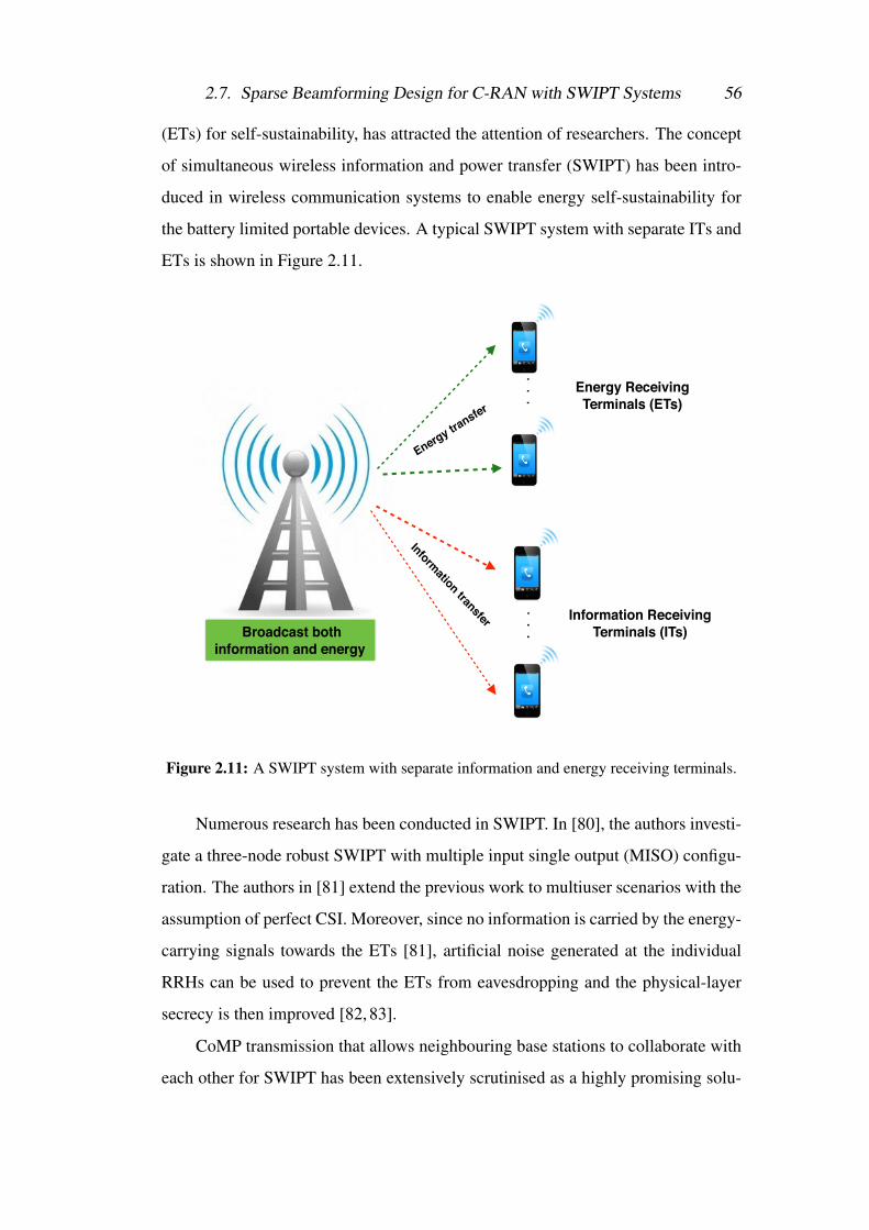
2.7. Sparse Beamforming Design for C-RAN with SWIPT Systems 56
(ETs) for self-sustainability, has attracted the attention of researchers. The concept
of simultaneous wireless information and power transfer (SWIPT) has been intro-
duced in wireless communication systems to enable energy self-sustainability for
the battery limited portable devices. A typical SWIPT system with separate ITs and
ETs is shown in Figure 2.11.
Broadcast both !information and energy
. . .
. . .
Energy Receiving !Terminals (ETs)
Information Receiving !Terminals (ITs)
Energy transfer
Information transfer
Figure 2.11: A SWIPT system with separate information and energy receiving terminals.
Numerous research has been conducted in SWIPT. In [80], the authors investi-
gate a three-node robust SWIPT with multiple input single output (MISO) configu-
ration. The authors in [81] extend the previous work to multiuser scenarios with the
assumption of perfect CSI. Moreover, since no information is carried by the energy-
carrying signals towards the ETs [81], artificial noise generated at the individual
RRHs can be used to prevent the ETs from eavesdropping and the physical-layer
secrecy is then improved [82, 83].
CoMP transmission that allows neighbouring base stations to collaborate with
each other for SWIPT has been extensively scrutinised as a highly promising solu-
2.7. Sparse Beamforming Design for C-RAN with SWIPT Systems 57
tion for ICI mitigation [10,84]. It has been proven that the total transmit power in a
CoMP transmission is reduced when a full cooperation is enabled [21]. However, if
all the RRHs in a C-RAN cooperate to transfer energy to all ETs and share the in-
formation of all ITs, huge fronthaul capacity is needed [8]. In practice, all the RRHs
in a C-RAN are connected with a cloud computing centralized unit via rate-limited
fronthaul links. Therefore, full cooperation may be infeasible.
All the aforementioned solutions have sparked interest among telecommunica-
tion researchers to investigate multi-cell cooperation transmission with restricted
fronthaul capacity [11–14, 18, 85–91] motivated by the remarkable performance
of reweighted `1-norm minimisation algorithm in compressing sensing introduced
in [9]. These studies proposed an iterative sparse beamforming algorithm to lessen
the load of the fronthaul links and used `1-norm of the beamforming vector to ap-
proximate the cluster size. Interestingly, [13] adopted a new weight factor updating
rule and achieved a better tradeoff between the total power transmit from all BSs
and the sum fronthaull capacity.
However, most of the sparse beamforming literatures cited above do not con-
sider the existence of energy harvesting devices and renewable energy productions
for the green network. In [10], the resource allocation algorithm design for a CoMP-
SWIPT network is proposed by optimising the transmit beamforming vectors at the
CP and energy sharing between the CP and RRHs. This architecture however, does
not consider renewable energy resources that can be further extended for energy
cooperation and energy trading in the C-RAN with SWIPT network.
The data circulation between the CP and the RRHs for full coordination re-
quires huge fronthaul signalling overhead, which may be infeasible in practice.
Therefore, motivated by reweighted `1-norm convex relaxation in compressive sens-
ing, the authors in [10,13] proposed dynamic iterative sparse beamforming designs
with QoS constraints for capacity-limited fronthaul links in CoMP systems.
Clustering techniques can reduce the estimation overhead and computational
complexity significantly by limiting the number of RRHs in one cluster, and thereby,
resulting to low capacity requirements on the fronthaul. However, these techniques
2.7. Sparse Beamforming Design for C-RAN with SWIPT Systems 58
have drawbacks where the C-RAN large-scale cooperative processing gains and
capacity will be reduced. Through these approaches, the centralized processing ca-
pability will not be optimized. Disjoint clustering and user-centric clustering are the
two classical types of RRH clustering schemes. In disjoint clustering architecture,
the C-RAN is categorized into non overlapping clusters, and RRHs in each cluster
jointly serve all receiving terminals within the coverage area. On contrary, receiv-
ing terminals at the cluster edge suffer from considerable inter-cluster interference
despite its effectiveness in combating the ICI. In user-centric clustering, each re-
ceiving terminal is served by an individually selected subset of neighbouring RRHs
and different clusters for different receiving terminals may overlap. The advantage
of this scheme is there is no explicit cluster edge. Such scheme can be further ex-
tended to two distinct implementations which relies heavily on the conditions of
RRH clustering, dynamic or static over different time slots. In dynamic user-centric
clustering, the RRH cluster for each receiving terminal can change over time, al-
lowing for more freedom to fully utilize the fronthaul resources. However, dynamic
user-centric clustering also requires a large amount of signalling overhead as new
receiving terminal associations need to be established continuously. Meanwhile,
in the static user-centric clustering, the receiving terminal association is fixed over
time and may only need to be updated as the receiving terminal location changes.
Dynamic clustering can outperform significantly the disjoint clustering strategy,
while heuristic static clustering schemes can achieve a substantial portion of the
performance gain.
The cluster size has been identified as one of the most critical design param-
eters for clustering scheme. Optimizing the dimension of cluster size can be made
possible through the following:
1. The cluster size determines the number of active RRHs at any time. This
leads to the density of active RRHs that controls the co-channel interference
coming from a scheduled receiving terminal.
2. The number of simultaneously schedules receiving terminals per unit area is
determined by the radius of the cluster.
2.8. Resource Management and Energy Trading with the Smart Grid 59
3. The dimensions of a cluster determine the number of RRHs serving a sched-
uled receiving terminal, leading to the diversity gain experienced due to spa-
tially distributed RRHs.
The derivative of viable successful access probability (SAP) has been made by ap-
plying stochastic geometry in [92]. In this work, the clustering of RRHs is formu-
lated as a coalitional game where a merge and split technique has been proposed
as an efficient solution through the theoretical result, in which represents a utility
function.
Look at different prospective and idea, the clustering of RRHs in this thesis is
optimized by using convex optimization technique because of its ability in solving
practical engineering problems reliably and efficiently. The strategies proposed in
this thesis are based on dynamic RRH-centric clustering, where the RRH cluster
for each receiving terminal is changed intelligently depending on the production of
renewable energy harvesters installed at each RRH, i.e., power budget. The size of
the RRH cluster is changed dynamically depending on its power budget with the
aim to minimize the total cost of the network operator as well as to address all the
given constraints.
2.8 Resource Management and Energy Trading with
the Smart GridEquipping the RRHs with renewable energy harvesting devices that can generate lo-
cal renewable energy from environmental sources, e.g., solar and wind, green com-
munications provide new perspective in reducing energy cost of cellular networks.
In practice, renewable energy generation is uneven due to the different efficiencies
of renewable energy harvesters and various RRHs installation sites. Therefore, the
power from the reliable source, i.e., power grid, is still needed to provide continu-
ous energy supply to all the RRHs in the C-RAN. Power supply from the smart grid
is always reliable but expensive because of time-varying energy prices.
Hybrid energy supply from both renewable energy devices and advanced smart
grid technology motivates a new idea of energy cooperation and energy trading in
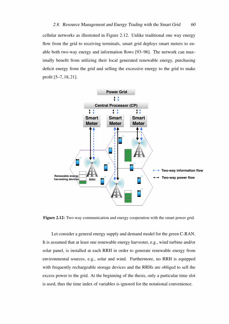
2.8. Resource Management and Energy Trading with the Smart Grid 60
cellular networks as illustrated in Figure 2.12. Unlike traditional one way energy
flow from the grid to receiving terminals, smart grid deploys smart meters to en-
able both two-way energy and information flows [93–96]. The network can max-
imally benefit from utilizing their local generated renewable energy, purchasing
deficit energy from the grid and selling the excessive energy to the grid to make
profit [5–7, 18, 21].
Renewable energy !harvesting devices RRH
Smart !Meter
Smart !Meter
Smart !Meter
Central Processor (CP)
Power Grid
Two-way power flow
Two-way information flow
Figure 2.12: Two-way communication and energy cooperation with the smart power grid.
Let consider a general energy supply and demand model for the green C-RAN.
It is assumed that at least one renewable energy harvester, e.g., wind turbine and/or
solar panel, is installed at each RRH in order to generate renewable energy from
environmental sources, e.g., solar and wind. Furthermore, no RRH is equipped
with frequently rechargeable storage devices and the RRHs are obliged to sell the
excess power to the grid. At the beginning of the thesis, only a particular time slot
is used, thus the time index of variables is ignored for the notational convenience.
2.8. Resource Management and Energy Trading with the Smart Grid 61
Let En, Bn and Sn denote the amount of renewable energy generated at the n-th
RRH, the amount of energy needed to be purchased from the grid by the n-th RRH
and the amount of excessive energy sold to the grid by the n-th RRH, respectively.
Furthermore, let P[Tx]n and P[circuit]
n indicate the total transmit power at the n-th RRH
and the hardware circuit power consumption at the n-th RRH, respectively. Then,
the total energy consumption at the n-th RRH, i.e., P[total]n , is upper-bounded by the
total available energy at the n-th RRH as follows
P[total]n = P[Tx]
n +P[circuit]n ≤ En +Bn−Sn. (2.32)
In practice, the price of generating per unit renewable energy π [renew] is much
cheaper than the price of purchasing per unit energy from the grid π [buy]. From the
supply and demand perspective, the RRH purchases additional energy from the grid
at a higher price π [buy] and sells the unconsumed energy to the grid at a reduced price
π [sell]. Intelligibly, π [buy] ≥ π [sell] ≥ π [renew] holds to avoid the trivial case where
any RRH in the cooperative network can make a profit by reselling the purchased
energy back to the grid or other RRHs. Note that, in this cooperative network, the
total energy purchased from the power grid by all the RRHs is the total renewable
energy deficit in the network. Thus, all the RRHs in the C-RAN can maximally
benefit from utilizing their local generated renewable energy to provide a green
network. As a result, the total energy cost of the cooperative RRHs, denoted by
B[total], can be calculated as
B[total] = π[renew]
∑n∈Lb
En +π[buy]
∑n∈Lb
Bn−π[sell]
∑n∈Lb
Sn, (2.33)
It is necessary to jointly optimize the resource allocation and energy trading
to guarantee the profit of the network operator and also to support green communi-
cation. To further reduce the total energy cost, a system should be embedded with
the intelligent algorithms to observe, learn and predict the energy that should be
purchased from the the grid.
2.9. Related Works 62
2.9 Related Works
Provided that all of the BSs are equipped with renewable energy harvesters and
implemented with two-way energy trading, [7, 21] propose a joint energy trading
and full cooperation scheme in CoMP network, where the data of all of the users
is available at the CP and will be distributed to all of the BSs in the cluster for co-
operative transmission via fronthaul links. However, the data circulation between
the CP and the BSs requires huge fronthaul signalling overhead when full coordi-
nation is enabled. The scheme, nevertheless, takes no account of fronthaul capacity
restrictions, which may be infeasible for practical capacity-constrained fronthaul
links [8]. Consequently, CoMP with finite fronthaul capacity has been investigated
by the scientific community and sparse beamforming technique for partial coopera-
tion is considered as a viable solution to this issue. Motivated by the literature that
sparse beamforming problem is commonly formulated as a `0-norm optimization
problem and handled with reweighted `1-norm method in the field of compressive
sensing [9], the authors in [11–14, 89] propose dynamic sparse beamforming de-
signs subject to QoS constraints for capacity-limited fronthaul links in CoMP net-
works. The authors in [10] integrate the aforementioned works with SWIPT concept
and study the resource allocation algorithm, under QoS constraints for information
receivers and power constraints at the BSs and the CP. It can be perceived that
sparse beamforming technique in joint cooperative real-time resource management
and energy trading problem in green C-RAN is firstly tackled in [18].
According to the theory of probability, a multi-armed bandit (MAB) is a prob-
lem in which a gambler at a row of slot machines has to make a decision on which
order and how many times the levers should be pulled to maximize the accumu-
lated reward, also known as linear or classic MAB [17]. In statistics and reinforce-
ment learning, the problem based on MAB concept has been well studied in the
literature [16, 97–100]. The research on stochastic MAB problem which is intro-
duced in [101] presents that under certain conditions on reward distributions, a tight
asymptotic regret of O(log n) can be obtained, where n is the number of rounds
played. Note that, regret is the metric for measuring the effectiveness of an MAB
2.9. Related Works 63
algorithm. Regret can be calculated as the difference in the total expected reward
between always playing the optimal arm and playing arms according to the algo-
rithm [16]. Then, [102] shows that O(log n) regret can be achieved uniformly over
time rather than only asymptotically in the other work [103]. The problem can be
categorized as a combinatorial MAB (CMAB) problem if multiple arms are pulled
simultaneously and the individual reward for each arm is observed [16]. The CMAB
problem has been studied intensively in [104–107].
However, none of this work applies the concept of CMAB in the real-time
resource management and energy trading between the C-RAN and the smart grid.
To employ an abstract idea of MAB for the CP to learn from the behaviour of the
energy trading in C-RAN iteratively, let consider each arm corresponds to the size
of an energy package to be purchased by the network operator from the day-ahead
market prior to the actual time of energy demand. Therefore, the new responsibility
of the CP is to find the set of optimal sizes of the energy packages to be purchased
from the day-ahead market without the initial knowledge of forthcoming instanta-
neous energy demand, in order to minimize the total energy cost of the network
operator. At each time instant, the CP learns from behaviour of cooperative energy
trading and predicts an amount of energy consumed by the individual RRH to fur-
ther minimize the amount of energy that should be purchased from the real-time
market, under the a set of constraints.
The other potential concept that can be applied in the real-time resource man-
agement and energy trading between the C-RAN and the smart grid is a game theo-
retical approach. Game theoretical approach is the study of optimal decision making
under competition when the decisions of one player in a team will effect the out-
come of a situation for all other players involved [94]. On the contrary, the MAB
problem models a slot machine attempts to maximize the accumulated reward by
iteratively optimizing the decisions among a set of arms based on existing knowl-
edge, known as exploitation, while simultaneously acquiring new knowledge by
observing the associated reward, known as exploration [17]. The MAB approach
can be jointly implemented with game theoretical approach to further motivate the
2.10. Concluding Remarks 64
potential RRHs with extra energy to assist in neighbourhood energy sharing and
trading. A practical energy and communication cooperation mechanism needs to be
designed for RRHs by the game theoretical approach. For example, the RRHs could
be selfish and prefer to store the harvested energy rather than to cooperate with the
other RRHs. In this situation, that particular RRHs need to be offered some extra
incentive to encourage them to be good players in a game. A good cooperation
mechanism design is required to motivate all the players in a system. This work
also can be extended to a huge network cooperation to support the inter-system
joint cooperation to a win-win situation for all the systems involved. This work is
an interesting direction for future research.
2.10 Concluding RemarksThis chapter begins with brief reviews on a C-RAN powered by renewable energy
technologies and a downlink beamforming design. Then, an optimization problem
for a downlink beamforming to calculate transmit beamformers for multiple receiv-
ing terminals in C-RAN with a constraint of power budget at each RRHs scenario
is introduced. A method to transform the non-convex optimization problem into
convex optimization problem using semidefinite programming forms is presented,
which can be effectively solved by available optimization packets. This chapter also
provides an overview on a resource management and energy trading approach for
energy cost saving in C-RAN powered by renewable energy sources and smart grid.
The two-way energy cooperation between the smart grid and the RRHs in a C-RAN
is expected to reshape the non-uniform energy supplies and energy demands over
the C-RAN for cost-saving. Hopefully, the technical background provided in this
chapter delivers the readers with the basic knowledge of the work areas to have
better understanding on the proposed problems in the forthcoming chapters.
Chapter 3
Real-Time Energy Management in
Green C-RAN
3.1 Introduction
With enormously increasing demand for mobile data and high data rates, the aggre-
gated power requirements by receiving terminals may exceed the amount of power
budget at the remote radio heads (RRHs). Hence, the network operator has to pur-
chase additional energy from the real-time market, i.e., the grid, and may take a risk
of losing the profit. To address the aforementioned issue, this chapter introduces
the real-time energy management for green cloud radio access networks (C-RANs)
using the local renewable energy generation at RRHs.
This chapter proposes three different cooperative real-time energy trading
strategies, namely, power-shortage management by partial cooperation, power-
shortage management by full cooperation, and overall network energy manage-
ment by full cooperation, to jointly minimize the energy consumption and the real-
time energy trading under the constraints of demand and supply power balancing at
RRHs and quality of service satisfaction at user terminals.
For the first strategy, a sparse beamforming problem is formulated as an `0-
norm optimization problem and solve it using semidefinite relaxation (SDR) and
iterative reweighted `1-norm approximation of `0-norm. The second and the third
strategies are formulated as numerically tractable optimization problems and solve
3.2. System Model 66
them using the SDR approach.
3.1.1 Organization
The remainder of this chapter is organized as follows. Section 3.2 presents the
system model. In section 3.3, 3.4 and 3.5, the formulations of Strategy 1: Power-
Shortage Management by Partial Cooperation, Strategy 2: Power-Shortage Man-
agement by Full Cooperation and Strategy 3: Overall Network Energy Manage-
ment by Full Cooperation, respectively, for cooperative real-time energy trading
are introduced. The resulting non-convex problems for all the proposed strategies
are reformulated and then transformed into tractable forms using convex relaxation.
Numerical simulation results are analyzed in section 3.6. Finally, section 3.7 sum-
marizes the chapter.
3.2 System ModelThis model considers a C-RAN with N RRHs, Ki single-antenna information re-
ceiving terminals (ITs) and a centralized cloud computing processor (CP). Let
Lb = {1, · · · ,N} and Li = {1, · · · ,Ki} denote, respectively, the set of indexes for
the RRHs and the ITs. The CP is the core processing unit in the system that designs
and broadcasts all the coordination strategies to the RRHs based on the perfect
knowledge of channel state information. The CP has also access to all the data for
the ITs and distributes them to all the RRHs for cooperative transmission of infor-
mation to the individual ITs. Each RRH is equipped with an array of M antenna
elements. Here, the energy transmission between the CP and RRHs in the system is
assumed to be accomplished via dedicated power lines.
3.2.1 Energy Management Model
From the perspective of capital expenditure (CAPEX) and operating expense
(OPEX), at least one renewable energy harvesting device, e.g., wind turbine and/or
solar panel, is assumed to be installed at the individual RRHs in order to generate
local renewable energy from environmental sources. Whereas, no RRH is equipped
with frequently rechargeable storage devices and the RRHs are obliged to transmit
the excessive power back to the CP for sale. In practice, the renewable energy gener-
3.2. System Model 67
ation is unequal due to efficiency of different types of renewable energy harvesting
devices and various RRHs locations. Let En, B[ahead]n , B[real]
n , Sn be defined, respec-
tively, as the amount of renewable energy generated at the n-th RRH, the amount
of energy that has been purchased from the day-ahead market for the n-th RRH,
the amount of energy that is necessary to be purchased from the real-time market
for the n-th RRH, and the amount of excessive energy sold back to the grid by the
n-th RRH. Furthermore, let P[Tx]n and P[circuit]
n indicate the total transmit power at
the n-th RRH and the non-transmission hardware circuit power consumption at the
n-th RRH, respectively. Then, the total energy consumption at the n-th RRH, i.e.,
P[total]n , is upper-bounded by the total available energy at the n-th RRH, i.e.,
P[total]n = P[Tx]
n +P[circuit]n ≤ En +B[ahead]
n +B[real]n −Sn. (3.1)
In practice, the price of generating per unit renewable energy, denoted by π [renew],
is much cheaper than the price of purchasing per unit energy from the day-ahead
market, represented by π [ahead]. From the supply and demand’s perspective, it is
assumed that the RRH purchases additional energy from the real-time market at a
higher price π [real] and sells the unconsumed energy back to the grid at a reduced
price π [sell], i.e., π [real] ≥ π [ahead] ≥ π [sell] ≥ π [renew]. Consequently, the total energy
cost of all the RRHs in the green C-RAN, denoted by B[total], is given by
B[total] = π[ahead]
∑n∈Lb
B[ahead]n +π
[real]∑
n∈Lb
B[real]n
+π[renew]
∑n∈Lb
En−π[sell]
∑n∈Lb
Sn. (3.2)
Thus, it is necessary to jointly optimize the resource allocation and energy trading
to guarantee the profit of the network operator.
3.2.2 Downlink Transmission Model
Let denote the aggregate beamformer from all RRHs towards the k-th IT as wk =
[wH1k, · · · ,wH
Nk]H ∈ CMN×1, where wnk ∈ CM×1 is the beamforming vector from the
n-th RRH to the k-th IT, k ∈Li. Similarly, the aggregate channel between all RRHs
3.2. System Model 68
and the k-th IT is denoted as hk = [hH1k, · · · ,hH
Nk]H ∈ CMN×1, where hnk ∈ CM×1 is
the channel vector between the n-th RRH and the k-th IT, k ∈ Li. The received
signal at the k-th IT, k ∈Li is given by
zk = hHk wksk + ∑
j 6=khH
k w js j +nk, ∀k ∈Li (3.3)
where sk indicates the data symbol for the k-th IT and nk ∼CN(0,σ2k ) is the additive
white Gaussian noise at the k-th IT. Without loss of generality, it is assumed that the
noise variance σ2k is identical at all ITs and E(|sk|2) = 1, ∀k ∈Li. Then, the signal-
to-interference-plus-noise ratio (SINR) at the k-th IT can be expressed as
SINRk =|hH
k wk|2∑j 6=k|hH
k w j|2 +σ2s, ∀k ∈Li. (3.4)
The shortage of power budget occurs when the aggregate available power at a
RRH is insufficient to satisfy the demand of multiple ITs. As a result, it is necessary
for the network operator to purchase the additional energy from the real-time market
at a higher price, which, consequently, may increase the total cost of the network
operator. Let Z = {1, · · · ,Z}, where Z ⊂Lb, indicate the set of indexes for the
RRHs that are in the shortage of power. Let say that the z-th RRH is in the shortage
of power, if its power budget denoted by P[budget]z is upper-bounded as
P[budget]z ≤
∑n∈Lb
(En +B[ahead]
n −P[circuit]n
)N
, ∀z ∈Z . (3.5)
In addition, let assume that the CP is frequently updated with the information of
all the RRHs’ power budgets, so that the indexes of RRHs that are in shortage
of power budget can be calculated in accordance with (3.5). Subsequently, the
optimal user cluster to be served by the RRHs with shortage of power budget, is
determined by the CP through evaluation of actual situations, e.g., the location of
ITs, the associated channel conditions and power budgets of the RRHs. In this
thesis, information of all the RRHs’ power budget are reliable. On the contrary,
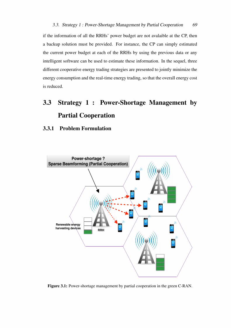
3.3. Strategy 1 : Power-Shortage Management by Partial Cooperation 69
if the information of all the RRHs’ power budget are not avalaible at the CP, then
a backup solution must be provided. For instance, the CP can simply estimated
the current power budget at each of the RRHs by using the previous data or any
intelligent software can be used to estimate these information. In the sequel, three
different cooperative energy trading strategies are presented to jointly minimize the
energy consumption and the real-time energy trading, so that the overall energy cost
is reduced.
3.3 Strategy 1 : Power-Shortage Management by
Partial Cooperation
3.3.1 Problem Formulation
Power-shortage ? Sparse Beamforming (Partial Cooperation)
Renewable energy harvesting devices RRH
Figure 3.1: Power-shortage management by partial cooperation in the green C-RAN.
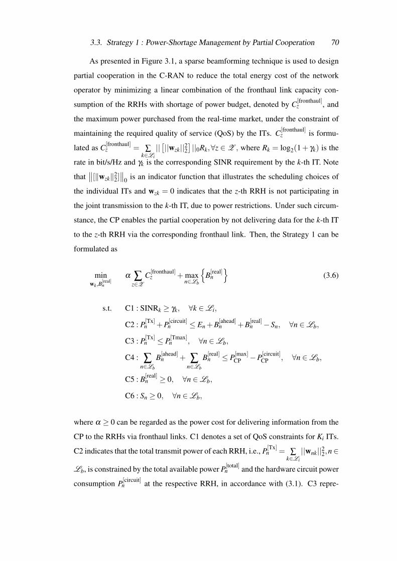
3.3. Strategy 1 : Power-Shortage Management by Partial Cooperation 70
As presented in Figure 3.1, a sparse beamforming technique is used to design
partial cooperation in the C-RAN to reduce the total energy cost of the network
operator by minimizing a linear combination of the fronthaul link capacity con-
sumption of the RRHs with shortage of power budget, denoted by C[fronthaul]z , and
the maximum power purchased from the real-time market, under the constraint of
maintaining the required quality of service (QoS) by the ITs. C[fronthaul]z is formu-
lated as C[fronthaul]z = ∑
k∈Li
||[||wzk||22
]||0Rk,∀z ∈Z , where Rk = log2(1+ γk) is the
rate in bit/s/Hz and γk is the corresponding SINR requirement by the k-th IT. Note
that∥∥[‖wzk‖2
2]∥∥
0 is an indicator function that illustrates the scheduling choices of
the individual ITs and wzk = 0 indicates that the z-th RRH is not participating in
the joint transmission to the k-th IT, due to power restrictions. Under such circum-
stance, the CP enables the partial cooperation by not delivering data for the k-th IT
to the z-th RRH via the corresponding fronthaul link. Then, the Strategy 1 can be
formulated as
minwk,B
[real]n
α ∑z∈Z
C[fronthaul]z + max
n∈Lb
{B[real]
n
}(3.6)
s.t. C1 : SINRk ≥ γk, ∀k ∈Li,
C2 : P[Tx]n +P[circuit]
n ≤ En +B[ahead]n +B[real]
n −Sn, ∀n ∈Lb,
C3 : P[Tx]n ≤ P[Tmax]
n , ∀n ∈Lb,
C4 : ∑n∈Lb
B[ahead]n + ∑
n∈Lb
B[real]n ≤ P[max]
CP −P[circuit]CP , ∀n ∈Lb,
C5 : B[real]n ≥ 0, ∀n ∈Lb,
C6 : Sn ≥ 0, ∀n ∈Lb,
where α ≥ 0 can be regarded as the power cost for delivering information from the
CP to the RRHs via fronthaul links. C1 denotes a set of QoS constraints for Ki ITs.
C2 indicates that the total transmit power of each RRH, i.e., P[Tx]n = ∑
k∈Li
||wnk||22,n∈
Lb, is constrained by the total available power P[total]n and the hardware circuit power
consumption P[circuit]n at the respective RRH, in accordance with (3.1). C3 repre-
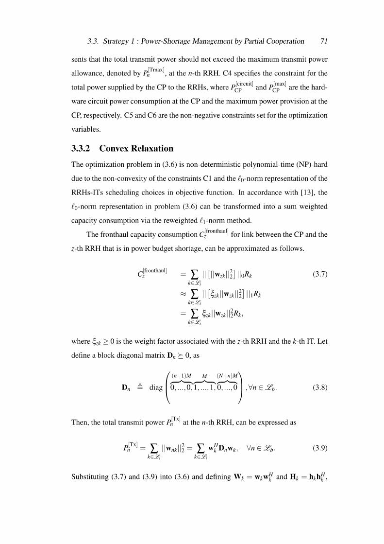
3.3. Strategy 1 : Power-Shortage Management by Partial Cooperation 71
sents that the total transmit power should not exceed the maximum transmit power
allowance, denoted by P[Tmax]n , at the n-th RRH. C4 specifies the constraint for the
total power supplied by the CP to the RRHs, where P[circuit]CP and P[max]
CP are the hard-
ware circuit power consumption at the CP and the maximum power provision at the
CP, respectively. C5 and C6 are the non-negative constraints set for the optimization
variables.
3.3.2 Convex Relaxation
The optimization problem in (3.6) is non-deterministic polynomial-time (NP)-hard
due to the non-convexity of the constraints C1 and the `0-norm representation of the
RRHs-ITs scheduling choices in objective function. In accordance with [13], the
`0-norm representation in problem (3.6) can be transformed into a sum weighted
capacity consumption via the reweighted `1-norm method.
The fronthaul capacity consumption C[fronthaul]z for link between the CP and the
z-th RRH that is in power budget shortage, can be approximated as follows.
C[fronthaul]z = ∑
k∈Li
||[||wzk||22
]||0Rk (3.7)
≈ ∑k∈Li
||[ξzk||wzk||22
]||1Rk
= ∑k∈Li
ξzk||wzk||22Rk,
where ξzk ≥ 0 is the weight factor associated with the z-th RRH and the k-th IT. Let
define a block diagonal matrix Dn � 0, as
Dn , diag
(n−1)M︷ ︸︸ ︷0, ...,0,
M︷ ︸︸ ︷1, ...,1,
(N−n)M︷ ︸︸ ︷0, ...,0
,∀n ∈Lb. (3.8)
Then, the total transmit power P[Tx]n at the n-th RRH, can be expressed as
P[Tx]n = ∑
k∈Li
||wnk||22 = ∑k∈Li
wHk Dnwk, ∀n ∈Lb. (3.9)
Substituting (3.7) and (3.9) into (3.6) and defining Wk = wkwHk and Hk = hkhH
k ,
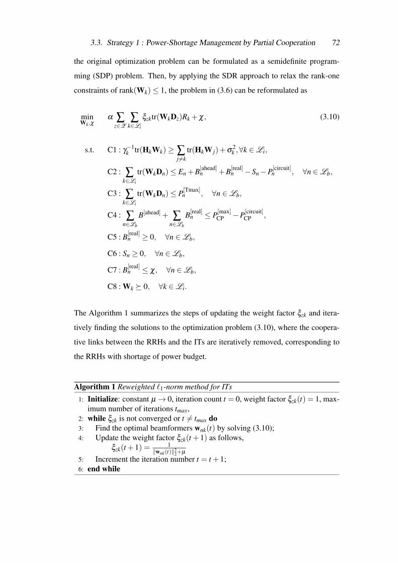
3.3. Strategy 1 : Power-Shortage Management by Partial Cooperation 72
the original optimization problem can be formulated as a semidefinite program-
ming (SDP) problem. Then, by applying the SDR approach to relax the rank-one
constraints of rank(Wk)≤ 1, the problem in (3.6) can be reformulated as
minWk,χ
α ∑z∈Z
∑k∈Li
ξzktr(WkDz)Rk +χ, (3.10)
s.t. C1 : γ−1k tr(HkWk)≥ ∑
j 6=ktr(HkW j)+σ
2k ,∀k ∈Li,
C2 : ∑k∈Li
tr(WkDn)≤ En +B[ahead]n +B[real]
n −Sn−P[circuit]n , ∀n ∈Lb,
C3 : ∑k∈Li
tr(WkDn)≤ P[Tmax]n , ∀n ∈Lb,
C4 : ∑n∈Lb
B[ahead]+ ∑n∈Lb
B[real]n ≤ P[max]
CP −P[circuit]CP ,
C5 : B[real]n ≥ 0, ∀n ∈Lb,
C6 : Sn ≥ 0, ∀n ∈Lb,
C7 : B[real]n ≤ χ, ∀n ∈Lb,
C8 : Wk � 0, ∀k ∈Li.
The Algorithm 1 summarizes the steps of updating the weight factor ξzk and itera-
tively finding the solutions to the optimization problem (3.10), where the coopera-
tive links between the RRHs and the ITs are iteratively removed, corresponding to
the RRHs with shortage of power budget.
Algorithm 1 Reweighted `1-norm method for ITs
1: Initialize: constant µ→ 0, iteration count t = 0, weight factor ξzk(t) = 1, max-imum number of iterations tmax,
2: while ξzk is not converged or t 6= tmax do3: Find the optimal beamformers wnk(t) by solving (3.10);4: Update the weight factor ξzk(t +1) as follows,
ξzk(t +1) = 1‖wnk(t)‖2
2+µ
5: Increment the iteration number t = t +1;6: end while
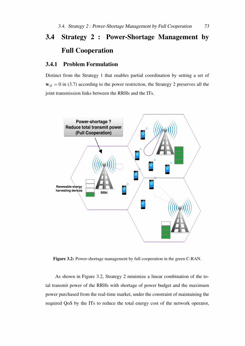
3.4. Strategy 2 : Power-Shortage Management by Full Cooperation 73
3.4 Strategy 2 : Power-Shortage Management by
Full Cooperation
3.4.1 Problem Formulation
Distinct from the Strategy 1 that enables partial coordination by setting a set of
wzk = 0 in (3.7) according to the power restriction, the Strategy 2 preserves all the
joint transmission links between the RRHs and the ITs.
Power-shortage ? Reduce total transmit power
(Full Cooperation)
Renewable energy harvesting devices RRH
Figure 3.2: Power-shortage management by full cooperation in the green C-RAN.
As shown in Figure 3.2, Strategy 2 minimize a linear combination of the to-
tal transmit power of the RRHs with shortage of power budget and the maximum
power purchased from the real-time market, under the constraint of maintaining the
required QoS by the ITs to reduce the total energy cost of the network operator,
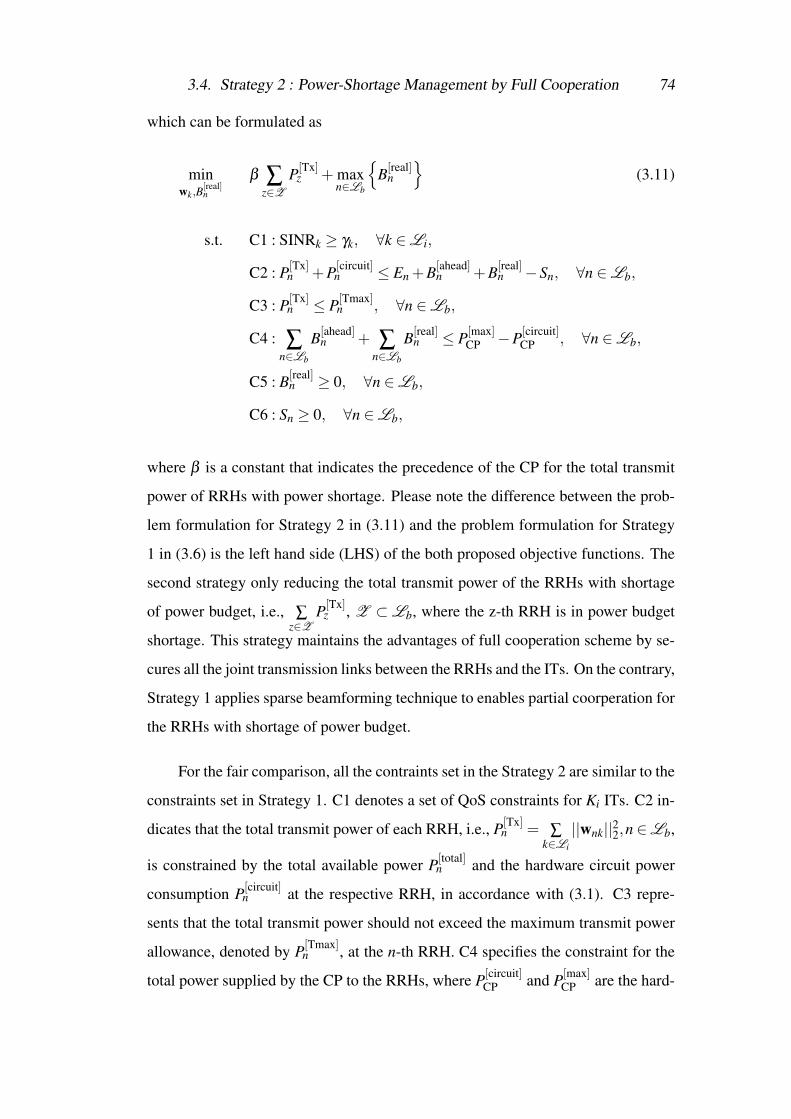
3.4. Strategy 2 : Power-Shortage Management by Full Cooperation 74
which can be formulated as
minwk,B
[real]n
β ∑z∈Z
P[Tx]z + max
n∈Lb
{B[real]
n
}(3.11)
s.t. C1 : SINRk ≥ γk, ∀k ∈Li,
C2 : P[Tx]n +P[circuit]
n ≤ En +B[ahead]n +B[real]
n −Sn, ∀n ∈Lb,
C3 : P[Tx]n ≤ P[Tmax]
n , ∀n ∈Lb,
C4 : ∑n∈Lb
B[ahead]n + ∑
n∈Lb
B[real]n ≤ P[max]
CP −P[circuit]CP , ∀n ∈Lb,
C5 : B[real]n ≥ 0, ∀n ∈Lb,
C6 : Sn ≥ 0, ∀n ∈Lb,
where β is a constant that indicates the precedence of the CP for the total transmit
power of RRHs with power shortage. Please note the difference between the prob-
lem formulation for Strategy 2 in (3.11) and the problem formulation for Strategy
1 in (3.6) is the left hand side (LHS) of the both proposed objective functions. The
second strategy only reducing the total transmit power of the RRHs with shortage
of power budget, i.e., ∑z∈Z
P[Tx]z , Z ⊂Lb, where the z-th RRH is in power budget
shortage. This strategy maintains the advantages of full cooperation scheme by se-
cures all the joint transmission links between the RRHs and the ITs. On the contrary,
Strategy 1 applies sparse beamforming technique to enables partial coorperation for
the RRHs with shortage of power budget.
For the fair comparison, all the contraints set in the Strategy 2 are similar to the
constraints set in Strategy 1. C1 denotes a set of QoS constraints for Ki ITs. C2 in-
dicates that the total transmit power of each RRH, i.e., P[Tx]n = ∑
k∈Li
||wnk||22,n ∈Lb,
is constrained by the total available power P[total]n and the hardware circuit power
consumption P[circuit]n at the respective RRH, in accordance with (3.1). C3 repre-
sents that the total transmit power should not exceed the maximum transmit power
allowance, denoted by P[Tmax]n , at the n-th RRH. C4 specifies the constraint for the
total power supplied by the CP to the RRHs, where P[circuit]CP and P[max]
CP are the hard-
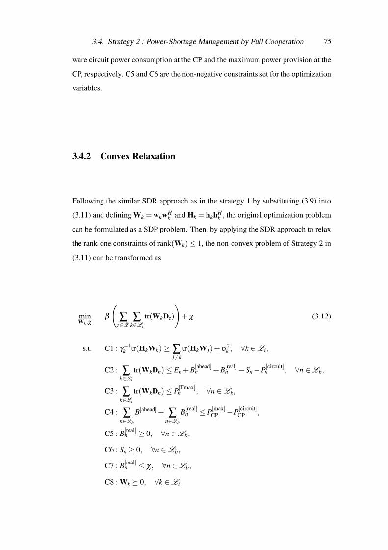
3.4. Strategy 2 : Power-Shortage Management by Full Cooperation 75
ware circuit power consumption at the CP and the maximum power provision at the
CP, respectively. C5 and C6 are the non-negative constraints set for the optimization
variables.
3.4.2 Convex Relaxation
Following the similar SDR approach as in the strategy 1 by substituting (3.9) into
(3.11) and defining Wk = wkwHk and Hk = hkhH
k , the original optimization problem
can be formulated as a SDP problem. Then, by applying the SDR approach to relax
the rank-one constraints of rank(Wk)≤ 1, the non-convex problem of Strategy 2 in
(3.11) can be transformed as
minWk,χ
β
(∑
z∈Z∑
k∈Li
tr(WkDz)
)+χ (3.12)
s.t. C1 : γ−1k tr(HkWk)≥ ∑
j 6=ktr(HkW j)+σ
2k , ∀k ∈Li,
C2 : ∑k∈Li
tr(WkDn)≤ En +B[ahead]n +B[real]
n −Sn−P[circuit]n , ∀n ∈Lb,
C3 : ∑k∈Li
tr(WkDn)≤ P[Tmax]n , ∀n ∈Lb,
C4 : ∑n∈Lb
B[ahead]+ ∑n∈Lb
B[real]n ≤ P[max]
CP −P[circuit]CP ,
C5 : B[real]n ≥ 0, ∀n ∈Lb,
C6 : Sn ≥ 0, ∀n ∈Lb,
C7 : B[real]n ≤ χ, ∀n ∈Lb,
C8 : Wk � 0, ∀k ∈Li.
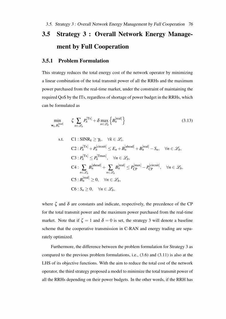
3.5. Strategy 3 : Overall Network Energy Management by Full Cooperation 76
3.5 Strategy 3 : Overall Network Energy Manage-
ment by Full Cooperation
3.5.1 Problem Formulation
This strategy reduces the total energy cost of the network operator by minimizing
a linear combination of the total transmit power of all the RRHs and the maximum
power purchased from the real-time market, under the constraint of maintaining the
required QoS by the ITs, regardless of shortage of power budget in the RRHs, which
can be formulated as
minwk,B
[real]n
ζ ∑n∈Lb
P[Tx]n +δ max
n∈Lb
{B[real]
n
}(3.13)
s.t. C1 : SINRk ≥ γk, ∀k ∈Li,
C2 : P[Tx]n +P[circuit]
n ≤ En +B[ahead]n +B[real]
n −Sn, ∀n ∈Lb,
C3 : P[Tx]n ≤ P[Tmax]
n , ∀n ∈Lb,
C4 : ∑n∈Lb
B[ahead]n + ∑
n∈Lb
B[real]n ≤ P[max]
CP −P[circuit]CP , ∀n ∈Lb,
C5 : B[real]n ≥ 0, ∀n ∈Lb,
C6 : Sn ≥ 0, ∀n ∈Lb,
where ζ and δ are constants and indicate, respectively, the precedence of the CP
for the total transmit power and the maximum power purchased from the real-time
market. Note that if ζ = 1 and δ = 0 is set, the strategy 3 will denote a baseline
scheme that the cooperative transmission in C-RAN and energy trading are sepa-
rately optimized.
Furthermore, the difference between the problem formulation for Strategy 3 as
compared to the previous problem formulations, i.e., (3.6) and (3.11) is also at the
LHS of its objective functions. With the aim to reduce the total cost of the network
operator, the third strategy proposed a model to minimize the total transmit power of
all the RRHs depending on their power budgets. In the other words, if the RRH has
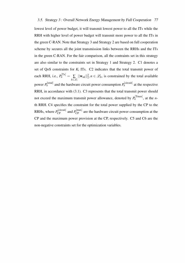
3.5. Strategy 3 : Overall Network Energy Management by Full Cooperation 77
lowest level of power budget, it will transmit lowest power to all the ITs while the
RRH with higher level of power budget will transmit more power to all the ITs in
the green C-RAN. Note that Strategy 3 and Strategy 2 are based on full cooperation
scheme by secures all the joint transmission links between the RRHs and the ITs
in the green C-RAN. For the fair comparison, all the contraints set in this strategy
are also similar to the constraints set in Strategy 1 and Strategy 2. C1 denotes a
set of QoS constraints for Ki ITs. C2 indicates that the total transmit power of
each RRH, i.e., P[Tx]n = ∑
k∈Li
||wnk||22,n ∈ Lb, is constrained by the total available
power P[total]n and the hardware circuit power consumption P[circuit]
n at the respective
RRH, in accordance with (3.1). C3 represents that the total transmit power should
not exceed the maximum transmit power allowance, denoted by P[Tmax]n , at the n-
th RRH. C4 specifies the constraint for the total power supplied by the CP to the
RRHs, where P[circuit]CP and P[max]
CP are the hardware circuit power consumption at the
CP and the maximum power provision at the CP, respectively. C5 and C6 are the
non-negative constraints set for the optimization variables.
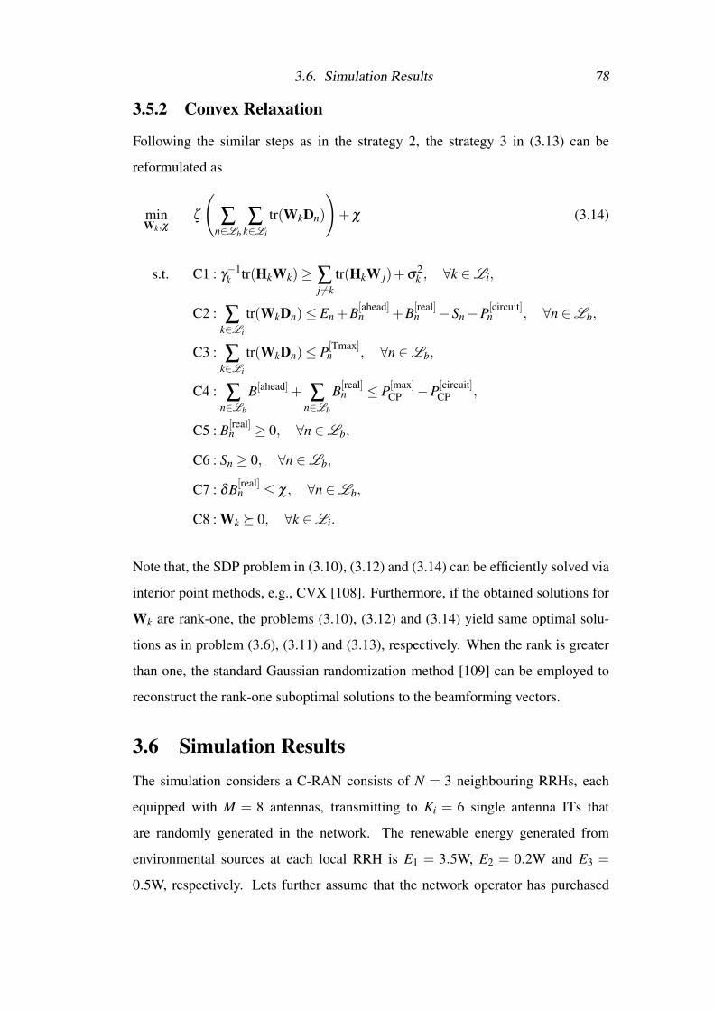
3.6. Simulation Results 78
3.5.2 Convex Relaxation
Following the similar steps as in the strategy 2, the strategy 3 in (3.13) can be
reformulated as
minWk,χ
ζ
(∑
n∈Lb
∑k∈Li
tr(WkDn)
)+χ (3.14)
s.t. C1 : γ−1k tr(HkWk)≥ ∑
j 6=ktr(HkW j)+σ
2k , ∀k ∈Li,
C2 : ∑k∈Li
tr(WkDn)≤ En +B[ahead]n +B[real]
n −Sn−P[circuit]n , ∀n ∈Lb,
C3 : ∑k∈Li
tr(WkDn)≤ P[Tmax]n , ∀n ∈Lb,
C4 : ∑n∈Lb
B[ahead]+ ∑n∈Lb
B[real]n ≤ P[max]
CP −P[circuit]CP ,
C5 : B[real]n ≥ 0, ∀n ∈Lb,
C6 : Sn ≥ 0, ∀n ∈Lb,
C7 : δB[real]n ≤ χ, ∀n ∈Lb,
C8 : Wk � 0, ∀k ∈Li.
Note that, the SDP problem in (3.10), (3.12) and (3.14) can be efficiently solved via
interior point methods, e.g., CVX [108]. Furthermore, if the obtained solutions for
Wk are rank-one, the problems (3.10), (3.12) and (3.14) yield same optimal solu-
tions as in problem (3.6), (3.11) and (3.13), respectively. When the rank is greater
than one, the standard Gaussian randomization method [109] can be employed to
reconstruct the rank-one suboptimal solutions to the beamforming vectors.
3.6 Simulation ResultsThe simulation considers a C-RAN consists of N = 3 neighbouring RRHs, each
equipped with M = 8 antennas, transmitting to Ki = 6 single antenna ITs that
are randomly generated in the network. The renewable energy generated from
environmental sources at each local RRH is E1 = 3.5W, E2 = 0.2W and E3 =
0.5W, respectively. Lets further assume that the network operator has purchased
3.6. Simulation Results 79
B[ahead]1 = B[ahead]
2 = B[ahead]3 = 1.5W amount of energy from the day-ahead mar-
ket at the price of π [ahead] = £0.07 per unit energy. If the energy is insufficient,
the network operator can purchase additional energy from the real-time market at
higher price of π [real] = £0.15 per unit energy while in the opposite case, the ex-
cessive energy can be sold back to the grid at a reduced price of π [sell] = £0.05
per unit energy. For simplicity, Let set P[circuit]n = 30dBm, P[circuit]
CP = 40dBm,
P[max]CP = 50dBm and P[Tmax]
n = 46dBm. Moreover, the distance between two ad-
jacent RRHs is D = 500m, and the channel bandwidth is chosen to be 20 MHz. A
correlated channel model is implemented, as suggested in [57], as hnk = R1/2nk hw,
where hw ∈ CM×1 are zero mean circularly symmetric complex Gaussian (ZMC-
SCG) random variables with unit variance, Rnk ∈ CM×M is the spatial covariance
matrix between the n-th RRH and the k-th IT, and the (m,n)-th element is given by
Rnk = GaLnkσ2Fe−0.5 (σs ln10)2
100 e j 2πδ
λ[(n−m)sinθnk]e−2[ πδσ
λ(n−m)cosθnk]
2
, where Ga = 15dBi
is the antenna gain, Lnk(dB)=125.2 +36.3log10(d) is the path loss between the n-th
RRH and the k-th IT, as suggested in 3GPP [63], σ2F is the variance of the complex
Gaussian fading coefficient, σs = 8dB is the standard deviation of the log-normal
fading (shadowing), δ = λ/2 is the spacing between two adjacent antenna elements,
λ is the wavelength of the carrier, σ = 2◦ is the angular offset standard deviation
and θnk is the estimated angle of departure between the n-th RRH and the k-th IT.
The list of parameters used in this simulation are summarized in Table 3.1. The
simulation results are averaged over 200 independent channel realizations.
Note that in Strategy 2, β is a constant that indicates the precedence of the CP
for the total transmit power of RRHs with power shortage. This strategy minimize a
linear combination of the total transmit power of the RRHs with shortage of power
budget and the maximum power purchased from the real-time market, under the
constraint of maintaining the required QoS by the ITs to reduce the total energy
cost of the network operator. Strategy 2(β = 1) and Strategy 2(β = 10) have been
chosen to study the impact of different weighting factor on the RRHs with shortage
of power budget. Figure 3.3 compares the performance of the proposed three joint
cooperative energy trading strategies with different parameter settings against the
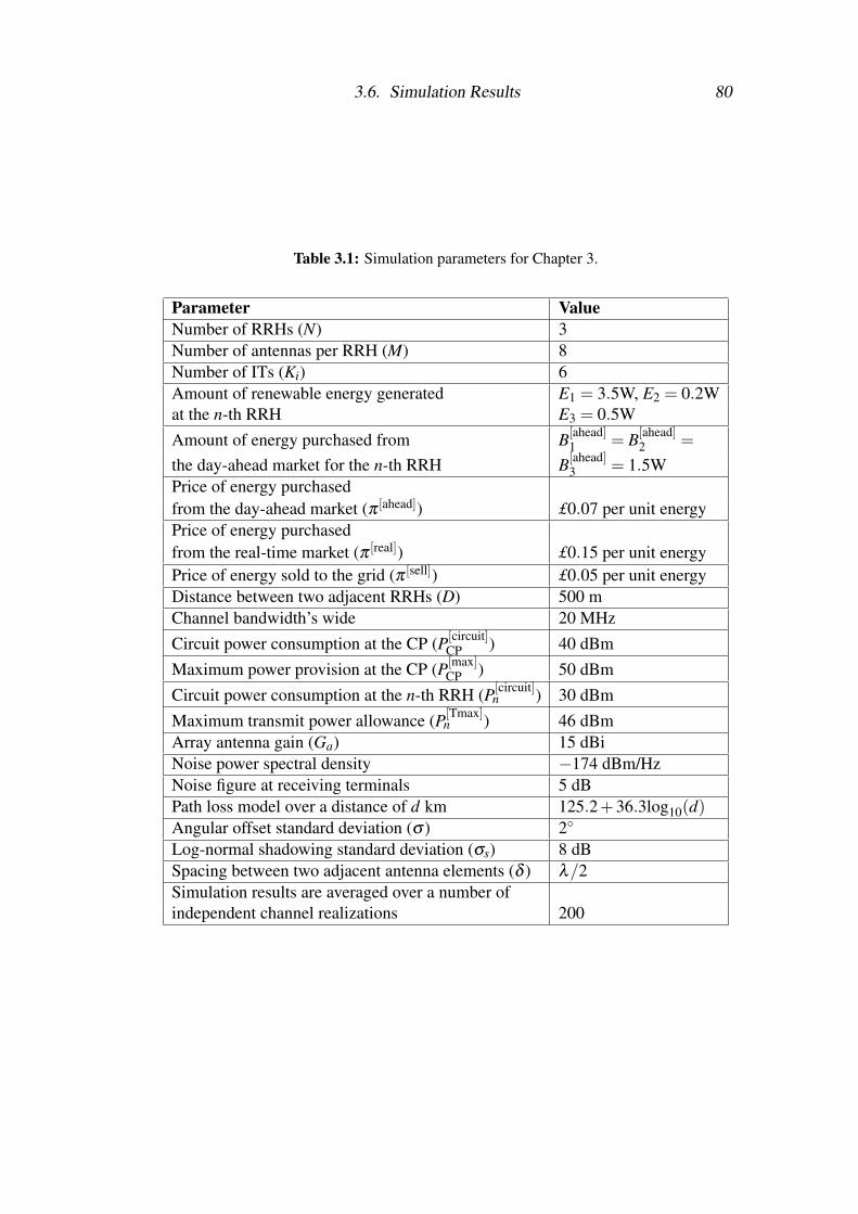
3.6. Simulation Results 80
Table 3.1: Simulation parameters for Chapter 3.
Parameter ValueNumber of RRHs (N) 3Number of antennas per RRH (M) 8Number of ITs (Ki) 6Amount of renewable energy generated E1 = 3.5W, E2 = 0.2Wat the n-th RRH E3 = 0.5WAmount of energy purchased from B[ahead]
1 = B[ahead]2 =
the day-ahead market for the n-th RRH B[ahead]3 = 1.5W
Price of energy purchasedfrom the day-ahead market (π [ahead]) £0.07 per unit energyPrice of energy purchasedfrom the real-time market (π [real]) £0.15 per unit energyPrice of energy sold to the grid (π [sell]) £0.05 per unit energyDistance between two adjacent RRHs (D) 500 mChannel bandwidth’s wide 20 MHzCircuit power consumption at the CP (P[circuit]
CP ) 40 dBmMaximum power provision at the CP (P[max]
CP ) 50 dBmCircuit power consumption at the n-th RRH (P[circuit]
n ) 30 dBmMaximum transmit power allowance (P[Tmax]
n ) 46 dBmArray antenna gain (Ga) 15 dBiNoise power spectral density −174 dBm/HzNoise figure at receiving terminals 5 dBPath loss model over a distance of d km 125.2+36.3log10(d)Angular offset standard deviation (σ ) 2◦
Log-normal shadowing standard deviation (σs) 8 dBSpacing between two adjacent antenna elements (δ ) λ/2Simulation results are averaged over a number ofindependent channel realizations 200
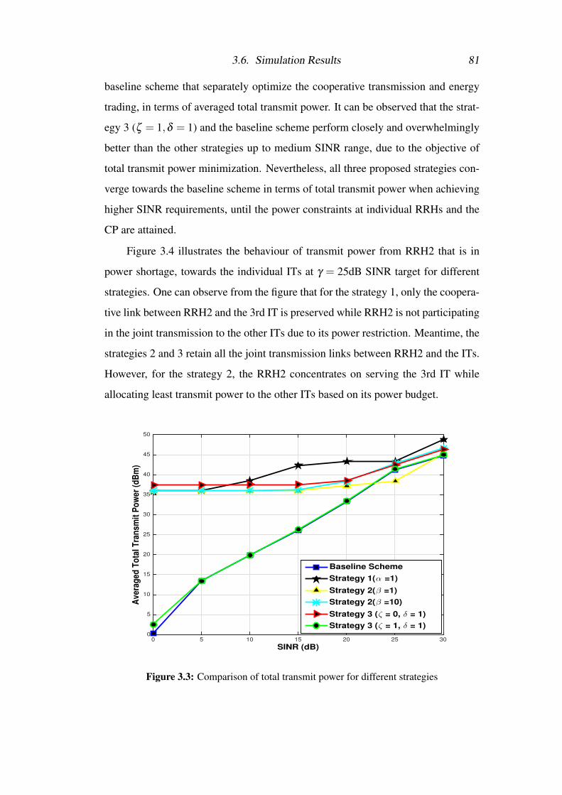
3.6. Simulation Results 81
baseline scheme that separately optimize the cooperative transmission and energy
trading, in terms of averaged total transmit power. It can be observed that the strat-
egy 3 (ζ = 1,δ = 1) and the baseline scheme perform closely and overwhelmingly
better than the other strategies up to medium SINR range, due to the objective of
total transmit power minimization. Nevertheless, all three proposed strategies con-
verge towards the baseline scheme in terms of total transmit power when achieving
higher SINR requirements, until the power constraints at individual RRHs and the
CP are attained.
Figure 3.4 illustrates the behaviour of transmit power from RRH2 that is in
power shortage, towards the individual ITs at γ = 25dB SINR target for different
strategies. One can observe from the figure that for the strategy 1, only the coopera-
tive link between RRH2 and the 3rd IT is preserved while RRH2 is not participating
in the joint transmission to the other ITs due to its power restriction. Meantime, the
strategies 2 and 3 retain all the joint transmission links between RRH2 and the ITs.
However, for the strategy 2, the RRH2 concentrates on serving the 3rd IT while
allocating least transmit power to the other ITs based on its power budget.
SINR (dB)0 5 10 15 20 25 30
Ave
rag
ed T
ota
l Tra
nsm
it P
ow
er (
dB
m)
0
5
10
15
20
25
30
35
40
45
50
Baseline Scheme
Strategy 1(α =1)
Strategy 2(β =1)
Strategy 2(β =10)
Strategy 3 (ζ = 0, δ = 1)
Strategy 3 (ζ = 1, δ = 1)
Figure 3.3: Comparison of total transmit power for different strategies
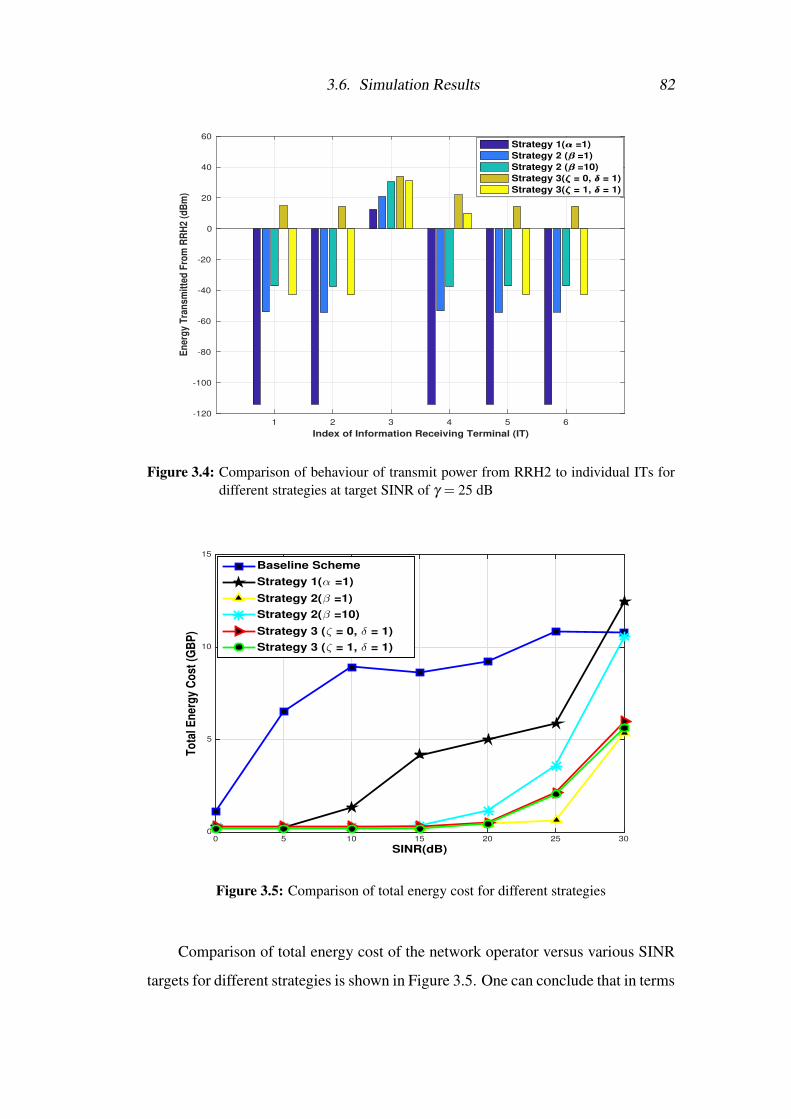
3.6. Simulation Results 82
1 2 3 4 5 6
Index of Information Receiving Terminal (IT)
-120
-100
-80
-60
-40
-20
0
20
40
60
En
erg
y T
ran
smit
ted
Fro
m R
RH
2 (d
Bm
)
Strategy 1( =1)
Strategy 2 ( =1)
Strategy 2 ( =10)
Strategy 3( = 0, = 1)
Strategy 3( = 1, = 1)
Figure 3.4: Comparison of behaviour of transmit power from RRH2 to individual ITs fordifferent strategies at target SINR of γ = 25 dB
SINR(dB)0 5 10 15 20 25 30
To
tal E
ner
gy
Co
st (
GB
P)
0
5
10
15
Baseline Scheme
Strategy 1(α =1)
Strategy 2(β =1)
Strategy 2(β =10)
Strategy 3 (ζ = 0, δ = 1)
Strategy 3 (ζ = 1, δ = 1)
Figure 3.5: Comparison of total energy cost for different strategies
Comparison of total energy cost of the network operator versus various SINR
targets for different strategies is shown in Figure 3.5. One can conclude that in terms
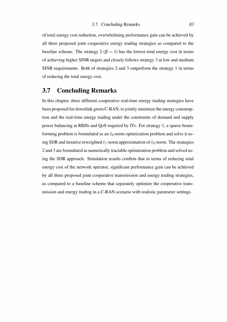
3.7. Concluding Remarks 83
of total energy cost reduction, overwhelming performance gain can be achieved by
all three proposed joint cooperative energy trading strategies as compared to the
baseline scheme. The strategy 2 (β = 1) has the lowest total energy cost in terms
of achieving higher SINR targets and closely follows strategy 3 at low and medium
SINR requirements. Both of strategies 2 and 3 outperform the strategy 1 in terms
of reducing the total energy cost.
3.7 Concluding RemarksIn this chapter, three different cooperative real-time energy trading strategies have
been proposed for downlink green C-RAN, to jointly minimize the energy consump-
tion and the real-time energy trading under the constraints of demand and supply
power balancing at RRHs and QoS required by ITs. For strategy 1, a sparse beam-
forming problem is formulated as an `0-norm optimization problem and solve it us-
ing SDR and iterative reweighted `1-norm approximation of `0-norm. The strategies
2 and 3 are formulated as numerically tractable optimization problem and solved us-
ing the SDR approach. Simulation results confirm that in terms of reducing total
energy cost of the network operator, significant performance gain can be achieved
by all three proposed joint cooperative transmission and energy trading strategies,
as compared to a baseline scheme that separately optimize the cooperative trans-
mission and energy trading in a C-RAN scenario with realistic parameter settings.
Chapter 4
Real-Time Energy Management in
Fronthaul Constrained Green
C-RAN
4.1 Introduction
In the practical downlink cloud radio access network (C-RAN), the tremendous in-
formation exchange between the centralized cloud computing processor (CP) and
the remote radio heads (RRHs) via capacity-constrained fronthaul links may result
in the infeasibility of full cooperation. Therefore, it is necessary to take into account
of the fronthaul capacity restrictions and employ sparse beamforming technique to
enable partial cooperation. However, the degree of partial cooperation among the
RRHs in serving the receiving terminals and the total transmit power minimiza-
tion conflict with each other. In particular, reducing the receiving terminal-RRH
cooperative links may be beneficial for fronthaul link capacity relaxation, it will,
nevertheless, result in an increase in the total transmit power. In the sequel, a joint
strategy of cooperative resource management and real-time energy trading is pro-
posed to strike an optimum balance between the total power consumption in the
fronthaul through adjusting the degree of partial cooperation among RRHs, RRHs’
total transmit power and their maximum or overall energy-purchase from real-time
market under the constraints of fronthaul link capacity restrictions. As shown in
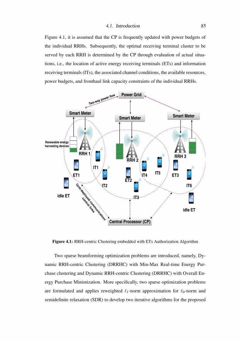
4.1. Introduction 85
Figure 4.1, it is assumed that the CP is frequently updated with power budgets of
the individual RRHs. Subsequently, the optimal receiving terminal cluster to be
served by each RRH is determined by the CP through evaluation of actual situa-
tions, i.e., the location of active energy receiving terminals (ETs) and information
receiving terminals (ITs), the associated channel conditions, the available resources,
power budgets, and fronthaul link capacity constraints of the individual RRHs.
Central Processor (CP)
Power Grid
Smart Meter Smart MeterSmart Meter
Two-way power flow
Grid-deployed communication/!
control links
Renewable energy !harvesting devices
IT1ET1
RRH 1RRH 2
RRH 3
IT2
IT5
IT3
IT4
idle ET
idle ET
IT6ET2
ET3
Figure 4.1: RRH-centric Clustering embedded with ETs Authorization Algorithm
Two sparse beamforming optimization problems are introduced, namely, Dy-
namic RRH-centric Clustering (DRRHC) with Min-Max Real-time Energy Pur-
chase clustering and Dynamic RRH-centric Clustering (DRRHC) with Overall En-
ergy Purchase Minimization. More specifically, two sparse optimization problems
are formulated and applies reweighted `1-norm approximation for `0-norm and
semidefinite relaxation (SDR) to develop two iterative algorithms for the proposed
4.1. Introduction 86
strategies.
In contrast to the energy management model proposed in the previous chapter
as well as in [18], this chapter integrates a real-time energy trading strategy with
simultaneous wireless information and power transfer (SWIPT) concept, where the
RRHs simultaneously transfer information beams to information receiving termi-
nals and energy beams to active energy receiving terminals. Since energy could
be highly attenuated over a long distance propagation and in order to maintain the
efficiency of SWIPT, an iterative ET authorization algorithm that allows only those
ETs situated close enough to the RRHs to receive wireless energy is introduced.
Instead of designing the sparse beamforming for individual RRHs with a short-
age of power proposed in Chapter 3, [18] and [21], the design strategies introduced
in this chapter account for all RRHs with or without a shortage of power. The pro-
posed strategies strike an optimum balance between the total power consumption
in the fronthaul through adjusting the degree of partial cooperation among RRHs,
RRHs’ total transmit power and their maximum or total energy-purchase from the
real-time market. More specifically, this chapter introduces two strategies for op-
timizing the RRHs’ real-time energy trading with the grid via: (1) minimizing the
RRHs’ maximum real-time energy-purchase requests; (2) minimizing the RRHs’
overall energy-purchase requests from the real-time market.
Unlike Chapter 3 and the latest papers for energy trading with grid, e.g.,
[7, 18, 21], that take no consideration of realistic constraints on fronthaul capac-
ity restrictions, this chapter formulates more realistic scenarios where RRHs are
constrained with limited fronthaul capacities. In practice, the fronthaul resources
are highly limited, especially, for joint transmission where all the users data are
circulated among all the RRHs. Hence, the designs that take no consideration of
fronthaul capacity constraints in problem formulation may lead to infeasible solu-
tions in practical scenarios.
The problem formulations naturally lead to computationally intractable opti-
mization problems which are dealt with in this chapter by reformulating the orig-
inal problems in their alternative tractable forms using rank relaxation technique,
4.2. System Model 87
i.e., SDR. The application of SDR adds a non-convex unit-rank constraints to the
alternative optimization problems, which are subsequently relaxed to find tractable
solutions. However, a randomization technique [60] which is a computationally
intensive search is required to pick only those feasible solutions that are unit-rank.
Attached in the Appendix A, this chapter analytically proves that the solutions to the
alternatively reformulated optimization problems using SDR are always unit-rank
and, hence, no subsequent search is required to find the unit-rank solutions.
4.1.1 Organization
The remainder of this chapter is organized as follows. Section 4.2 introduces the
system model and an iterative ET authorization algorithm. In section 4.3, the DR-
RHC with min-max energy purchase strategy is formulated, and then transformed
into numerically tractable form using reweighted `1-norm method and the SDR.
In section 4.4, the DRRHC with overall energy purchase minimization strategy is
proposed, and then transformed into numerically tractable form using reweighted
`1-norm method and the SDR. Numerical simulation results are analyzed in section
4.5. Finally, section 4.6 summarizes the chapter.
4.2 System ModelThis work considers a downlink C-RAN with SWIPT from N RRHs, equipped with
M antennas, towards Ki active single-antenna ITs and Ke active single-antenna ETs,
respectively, over the same frequency band. A CP is the core processing unit in the
network that coordinates all the cooperative strategies, e.g., cooperative energy trad-
ing, for the RRHs based on perfect knowledge of channel state information and real-
time supply and demand power balancing. Besides, the CP also has accessibility to
the data of all the ITs and distributes it along with beamformers, to the correspond-
ing RRHs via fronthaul links and collect the energy information, i.e., the energy
harvesting rates and energy buying/selling prices via the smart meters installed at
RRHs and the grid-deployed communication/control links connecting them. Let
Lb = {1, · · · ,N}, Le = {1, · · · ,Ke}, L [idle]e = {1, · · · ,K[idle]
e } and Li = {1, · · · ,Ki}indicate, respectively, the set of indexes of the RRHs, the active ETs, the idle ETs
4.2. System Model 88
and the active ITs. It is further assumed that the energy transmission between the
CP and the RRHs is accomplished via dedicated power lines.
4.2.1 Downlink Transmission Model
The aggregate beamforming vector from all the RRHs towards the i-th IT, i ∈Li,
as wi = [wH1i, · · · ,wH
Ni]H ∈CMN×1 is denoted, where wni ∈CM×1 is the beamformer
from the n-th RRH towards the i-th IT. ve = [vH1e, · · · ,vH
Ne]H ∈CMN×1 represents the
aggregate beamforming vector from all the RRHs to the e-th active ET. Similarly,
let hni ∈ CM×1 represent the channel vector between the n-th RRH and the i-th IT,
the aggregate channel vector between all the RRHs and the i-th IT is denoted by
hi = [hH1i, · · · ,hH
Ni]H ∈ CMN×1. The received signals at the i-th IT, i ∈ Li, is then
given by
yi = hHi wis
[IT]i + ∑
j 6=ij∈Li
hHi w js
[IT]j + ∑
e∈Le
hHi ves[ET]
e +ni, (4.1)
where the terms at the right hand side of (4.1), respectively, represent the intended
information-carrying signal for the i-th IT, the inter-user interference caused by
all other non-desired information beams, the interference caused by energy beams
for all active ETs and the additive white Gaussian noise, i.e., ni ∼ CN(0,σ2i ), at
the i-th IT. Since no information is carried by the energy-carrying signals, they
can be any arbitrary random signals. Without loss of generality, it is assumed that
E(s[IT]i ) = E(s[ET]
e ) = 1 and σ2i is identical at all receiving terminals. Then, the
signal-to-interference-plus-noise ratio (SINR) at the i-th IT, i ∈Li, is formulated as
SINR[IT]i =
|hHi wi|2
∑j∈Li, j 6=i
|hHi w j|2 + ∑
e∈Le
|hHi ve|2 +σ2
i. (4.2)
The fronthaul capacity consumption for the n-th RRH is given by
C[fronthaul]n = ∑
i∈Li
‖‖wni‖2‖0 Ri = ∑i∈Li
∥∥‖wni‖22∥∥
0 Ri, ∀n ∈Lb, (4.3)
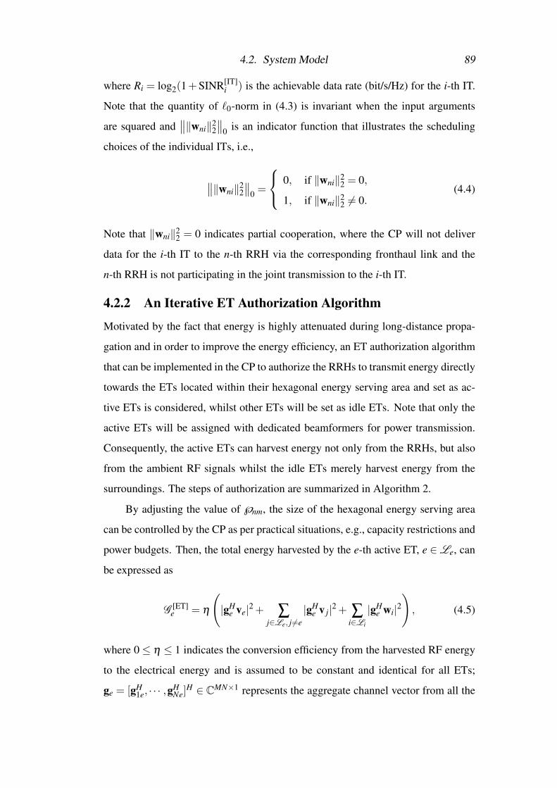
4.2. System Model 89
where Ri = log2(1+SINR[IT]i ) is the achievable data rate (bit/s/Hz) for the i-th IT.
Note that the quantity of `0-norm in (4.3) is invariant when the input arguments
are squared and∥∥‖wni‖2
2
∥∥0 is an indicator function that illustrates the scheduling
choices of the individual ITs, i.e.,
∥∥‖wni‖22∥∥
0 =
0, if ‖wni‖22 = 0,
1, if ‖wni‖22 6= 0.
(4.4)
Note that ‖wni‖22 = 0 indicates partial cooperation, where the CP will not deliver
data for the i-th IT to the n-th RRH via the corresponding fronthaul link and the
n-th RRH is not participating in the joint transmission to the i-th IT.
4.2.2 An Iterative ET Authorization Algorithm
Motivated by the fact that energy is highly attenuated during long-distance propa-
gation and in order to improve the energy efficiency, an ET authorization algorithm
that can be implemented in the CP to authorize the RRHs to transmit energy directly
towards the ETs located within their hexagonal energy serving area and set as ac-
tive ETs is considered, whilst other ETs will be set as idle ETs. Note that only the
active ETs will be assigned with dedicated beamformers for power transmission.
Consequently, the active ETs can harvest energy not only from the RRHs, but also
from the ambient RF signals whilst the idle ETs merely harvest energy from the
surroundings. The steps of authorization are summarized in Algorithm 2.
By adjusting the value of ℘nm, the size of the hexagonal energy serving area
can be controlled by the CP as per practical situations, e.g., capacity restrictions and
power budgets. Then, the total energy harvested by the e-th active ET, e ∈Le, can
be expressed as
G [ET]e = η
(|gH
e ve|2 + ∑j∈Le, j 6=e
|gHe v j|2 + ∑
i∈Li
|gHe wi|2
), (4.5)
where 0≤ η ≤ 1 indicates the conversion efficiency from the harvested RF energy
to the electrical energy and is assumed to be constant and identical for all ETs;
ge = [gH1e, · · · ,gH
Ne]H ∈ CMN×1 represents the aggregate channel vector from all the
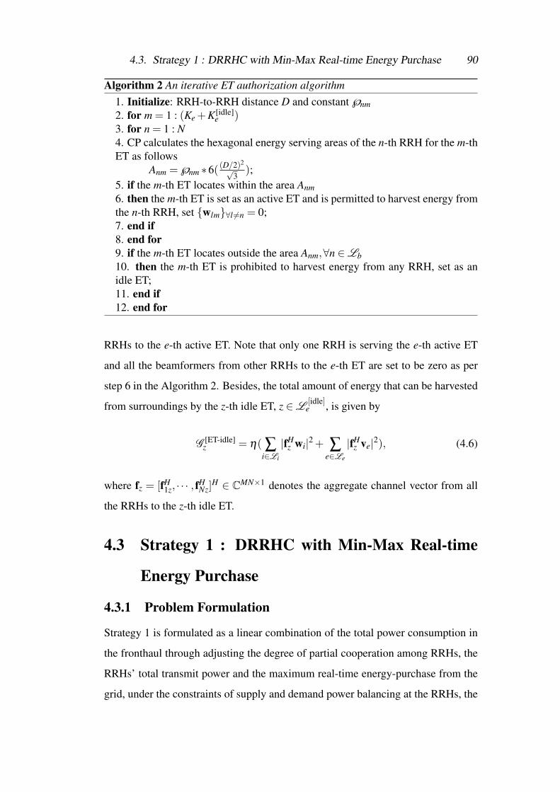
4.3. Strategy 1 : DRRHC with Min-Max Real-time Energy Purchase 90
Algorithm 2 An iterative ET authorization algorithm1. Initialize: RRH-to-RRH distance D and constant ℘nm2. for m = 1 : (Ke +K[idle]
e )3. for n = 1 : N4. CP calculates the hexagonal energy serving areas of the n-th RRH for the m-thET as follows
Anm =℘nm ∗6( (D/2)2√
3);
5. if the m-th ET locates within the area Anm6. then the m-th ET is set as an active ET and is permitted to harvest energy fromthe n-th RRH, set {wlm}∀l 6=n = 0;7. end if8. end for9. if the m-th ET locates outside the area Anm,∀n ∈Lb10. then the m-th ET is prohibited to harvest energy from any RRH, set as anidle ET;11. end if12. end for
RRHs to the e-th active ET. Note that only one RRH is serving the e-th active ET
and all the beamformers from other RRHs to the e-th ET are set to be zero as per
step 6 in the Algorithm 2. Besides, the total amount of energy that can be harvested
from surroundings by the z-th idle ET, z ∈L[idle]
e , is given by
G [ET-idle]z = η( ∑
i∈Li
|fHz wi|2 + ∑
e∈Le
|fHz ve|2), (4.6)
where fz = [fH1z, · · · , fH
Nz]H ∈ CMN×1 denotes the aggregate channel vector from all
the RRHs to the z-th idle ET.
4.3 Strategy 1 : DRRHC with Min-Max Real-time
Energy Purchase
4.3.1 Problem Formulation
Strategy 1 is formulated as a linear combination of the total power consumption in
the fronthaul through adjusting the degree of partial cooperation among RRHs, the
RRHs’ total transmit power and the maximum real-time energy-purchase from the
grid, under the constraints of supply and demand power balancing at the RRHs, the
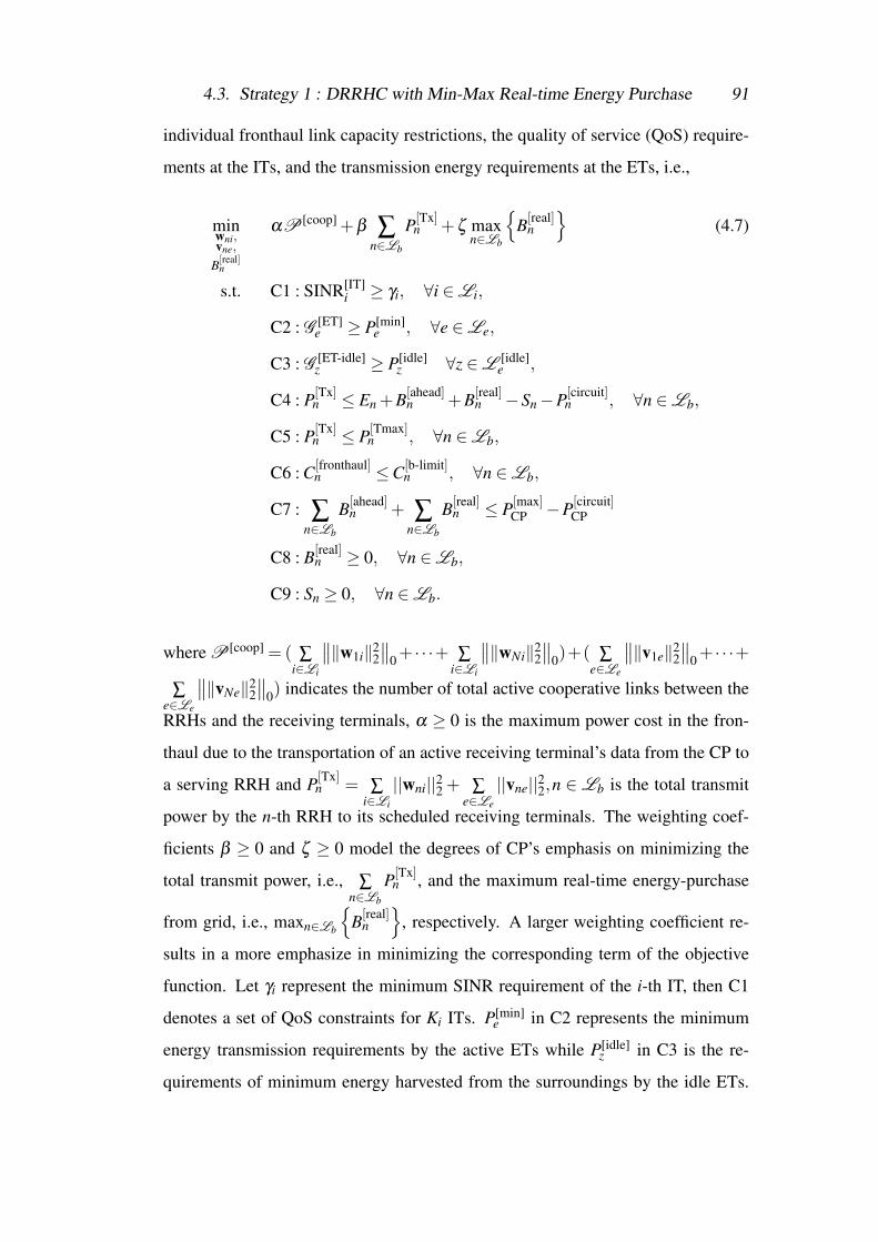
4.3. Strategy 1 : DRRHC with Min-Max Real-time Energy Purchase 91
individual fronthaul link capacity restrictions, the quality of service (QoS) require-
ments at the ITs, and the transmission energy requirements at the ETs, i.e.,
minwni,vne,
B[real]n
αP [coop] +β ∑n∈Lb
P[Tx]n +ζ max
n∈Lb
{B[real]
n
}(4.7)
s.t. C1 : SINR[IT]i ≥ γi, ∀i ∈Li,
C2 : G [ET]e ≥ P[min]
e , ∀e ∈Le,
C3 : G [ET-idle]z ≥ P[idle]
z ∀z ∈L [idle]e ,
C4 : P[Tx]n ≤ En +B[ahead]
n +B[real]n −Sn−P[circuit]
n , ∀n ∈Lb,
C5 : P[Tx]n ≤ P[Tmax]
n , ∀n ∈Lb,
C6 : C[fronthaul]n ≤C[b-limit]
n , ∀n ∈Lb,
C7 : ∑n∈Lb
B[ahead]n + ∑
n∈Lb
B[real]n ≤ P[max]
CP −P[circuit]CP
C8 : B[real]n ≥ 0, ∀n ∈Lb,
C9 : Sn ≥ 0, ∀n ∈Lb.
where P [coop] = ( ∑i∈Li
∥∥‖w1i‖22
∥∥0+ · · ·+ ∑
i∈Li
∥∥‖wNi‖22
∥∥0)+( ∑
e∈Le
∥∥‖v1e‖22
∥∥0+ · · ·+
∑e∈Le
∥∥‖vNe‖22
∥∥0) indicates the number of total active cooperative links between the
RRHs and the receiving terminals, α ≥ 0 is the maximum power cost in the fron-
thaul due to the transportation of an active receiving terminal’s data from the CP to
a serving RRH and P[Tx]n = ∑
i∈Li
||wni||22 + ∑e∈Le
||vne||22,n ∈Lb is the total transmit
power by the n-th RRH to its scheduled receiving terminals. The weighting coef-
ficients β ≥ 0 and ζ ≥ 0 model the degrees of CP’s emphasis on minimizing the
total transmit power, i.e., ∑n∈Lb
P[Tx]n , and the maximum real-time energy-purchase
from grid, i.e., maxn∈Lb
{B[real]
n
}, respectively. A larger weighting coefficient re-
sults in a more emphasize in minimizing the corresponding term of the objective
function. Let γi represent the minimum SINR requirement of the i-th IT, then C1
denotes a set of QoS constraints for Ki ITs. P[min]e in C2 represents the minimum
energy transmission requirements by the active ETs while P[idle]z in C3 is the re-
quirements of minimum energy harvested from the surroundings by the idle ETs.
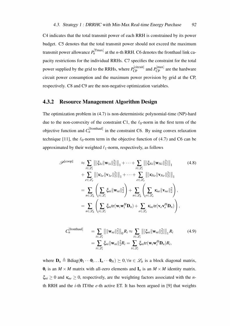
4.3. Strategy 1 : DRRHC with Min-Max Real-time Energy Purchase 92
C4 indicates that the total transmit power of each RRH is constrained by its power
budget. C5 denotes that the total transmit power should not exceed the maximum
transmit power allowance P[Tmax]n at the n-th RRH. C6 denotes the fronthaul link ca-
pacity restrictions for the individual RRHs. C7 specifies the constraint for the total
power supplied by the grid to the RRHs, where P[circuit]CP and P[max]
CP are the hardware
circuit power consumption and the maximum power provision by grid at the CP,
respectively. C8 and C9 are the non-negative optimization variables.
4.3.2 Resource Management Algorithm Design
The optimization problem in (4.7) is non-deterministic polynomial-time (NP)-hard
due to the non-convexity of the constraint C1, the `0-norm in the first term of the
objective function and C[fronthaul]n in the constraint C6. By using convex relaxation
technique [11], the `0-norm term in the objective function of (4.7) and C6 can be
approximated by their weighted `1-norm, respectively, as follows
P [coop] ≈ ∑i∈Li
∥∥[ξ1i‖w1i‖22]∥∥
1 + · · ·+ ∑i∈Li
∥∥[ξNi‖wNi‖22]∥∥
1 (4.8)
+ ∑e∈Le
∥∥[κ1e‖v1e‖22]∥∥
1 + · · ·+ ∑e∈Le
∥∥[κNe‖vNe‖22]∥∥
1
= ∑n∈Lb
(∑
i∈Li
ξni‖wni‖22
)+ ∑
n∈Lb
(∑
e∈Le
κne‖vne‖22
),
= ∑n∈Lb
(∑
i∈Li
ξnitr(wiwHi Dn)+ ∑
e∈Le
κnetr(vevHe Dn)
),
C[fronthaul]n = ∑
i∈Li
∥∥‖wni‖22∥∥
0 Ri ≈ ∑i∈Li
∥∥[ξni‖wni‖22]∥∥
1 Ri (4.9)
= ∑i∈Li
ξni‖wni‖22Ri = ∑
i∈Li
ξnitr(wiwHi Dn)Ri,
where Dn , Bdiag(01 · · ·0i . . .In · · ·0N) � 0,∀n ∈ Lb is a block diagonal matrix,
0i is an M×M matrix with all-zero elements and In is an M×M identity matrix.
ξni ≥ 0 and κne ≥ 0, respectively, are the weighting factors associated with the n-
th RRH and the i-th IT/the e-th active ET. It has been argued in [9] that weights
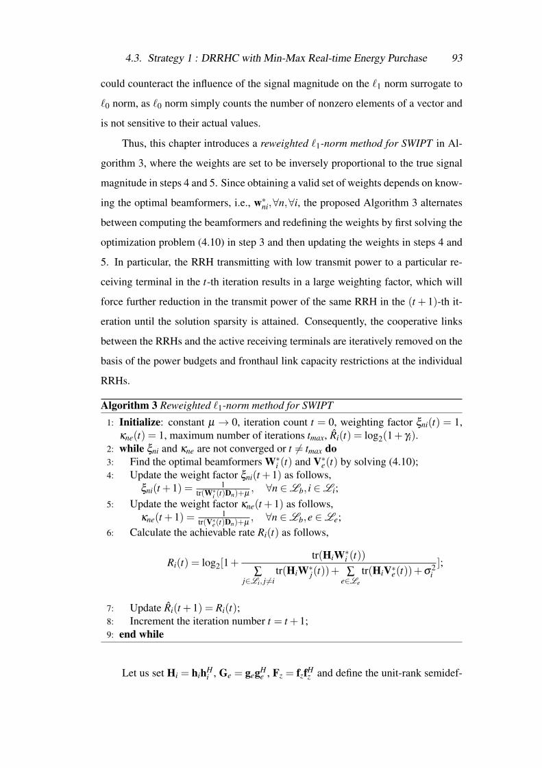
4.3. Strategy 1 : DRRHC with Min-Max Real-time Energy Purchase 93
could counteract the influence of the signal magnitude on the `1 norm surrogate to
`0 norm, as `0 norm simply counts the number of nonzero elements of a vector and
is not sensitive to their actual values.
Thus, this chapter introduces a reweighted `1-norm method for SWIPT in Al-
gorithm 3, where the weights are set to be inversely proportional to the true signal
magnitude in steps 4 and 5. Since obtaining a valid set of weights depends on know-
ing the optimal beamformers, i.e., w∗ni,∀n,∀i, the proposed Algorithm 3 alternates
between computing the beamformers and redefining the weights by first solving the
optimization problem (4.10) in step 3 and then updating the weights in steps 4 and
5. In particular, the RRH transmitting with low transmit power to a particular re-
ceiving terminal in the t-th iteration results in a large weighting factor, which will
force further reduction in the transmit power of the same RRH in the (t + 1)-th it-
eration until the solution sparsity is attained. Consequently, the cooperative links
between the RRHs and the active receiving terminals are iteratively removed on the
basis of the power budgets and fronthaul link capacity restrictions at the individual
RRHs.
Algorithm 3 Reweighted `1-norm method for SWIPT
1: Initialize: constant µ → 0, iteration count t = 0, weighting factor ξni(t) = 1,κne(t) = 1, maximum number of iterations tmax, Ri(t) = log2(1+ γi).
2: while ξni and κne are not converged or t 6= tmax do3: Find the optimal beamformers W∗i (t) and V∗e(t) by solving (4.10);4: Update the weight factor ξni(t +1) as follows,
ξni(t +1) = 1tr(W∗i (t)Dn)+µ
, ∀n ∈Lb, i ∈Li;5: Update the weight factor κne(t +1) as follows,
κne(t +1) = 1tr(V∗e(t)Dn)+µ
, ∀n ∈Lb,e ∈Le;6: Calculate the achievable rate Ri(t) as follows,
Ri(t) = log2[1+tr(HiW∗i (t))
∑j∈Li, j 6=i
tr(HiW∗j(t))+ ∑e∈Le
tr(HiV∗e(t))+σ2i];
7: Update Ri(t +1) = Ri(t);8: Increment the iteration number t = t +1;9: end while
Let us set Hi = hihHi , Ge = gegH
e , Fz = fzfHz and define the unit-rank semidef-
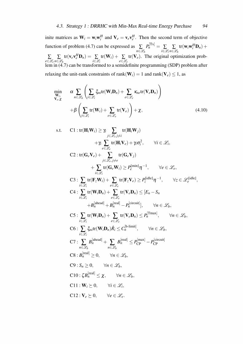
4.3. Strategy 1 : DRRHC with Min-Max Real-time Energy Purchase 94
inite matrices as Wi = wiwHi and Ve = vevH
e . Then the second term of objective
function of problem (4.7) can be expressed as ∑n∈Lb
P[Tx]n = ∑
i∈Li
∑n∈Lb
tr(wiwHi Dn)+
∑e∈Le
∑n∈Lb
tr(vevHe Dn) = ∑
i∈Li
tr(Wi)+ ∑e∈Le
tr(Ve). The original optimization prob-
lem in (4.7) can be transformed to a semidefinite programming (SDP) problem after
relaxing the unit-rank constraints of rank(Wi) = 1 and rank(Ve)≤ 1, as
minWi,
Ve,χ
α ∑n∈Lb
(∑
i∈Li
ξnitr(WiDn)+ ∑e∈Le
κnetr(VeDn)
)
+β
(∑
i∈Li
tr(Wi)+ ∑e∈Le
tr(Ve)
)+χ, (4.10)
s.t. C1 : tr(HiWi)≥ γi ∑j∈Li, j 6=i
tr(HiW j)
+γi ∑e∈Le
tr(HiVe)+ γiσ2i , ∀i ∈Li,
C2 : tr(GeVe)+ ∑j∈Le, j 6=e
tr(GeV j)
+ ∑i∈Li
tr(GeWi)≥ P[min]e η
−1, ∀e ∈Le,
C3 : ∑i∈Li
tr(FzWi)+ ∑e∈Le
tr(FzVe)≥ P[idle]z η
−1, ∀z ∈L [idle]e ,
C4 : ∑i∈Li
tr(WiDn)+ ∑e∈Le
tr(VeDn)≤ [En−Sn
+B[ahead]n +B[real]
n −P[circuit]n ], ∀n ∈Lb,
C5 : ∑i∈Li
tr(WiDn)+ ∑e∈Le
tr(VeDn)≤ P[Tmax]n , ∀n ∈Lb,
C6 : ∑i∈Li
ξnitr(WiDn)Ri ≤C[b-limit]n , ∀n ∈Lb,
C7 : ∑n∈Lb
B[ahead]n + ∑
n∈Lb
B[real]n ≤ P[max]
CP −P[circuit]CP
C8 : B[real]n ≥ 0, ∀n ∈Lb,
C9 : Sn ≥ 0, ∀n ∈Lb,
C10 : ζ B[real]n ≤ χ, ∀n ∈Lb,
C11 : Wi � 0, ∀i ∈Li,
C12 : Ve � 0, ∀e ∈Le.
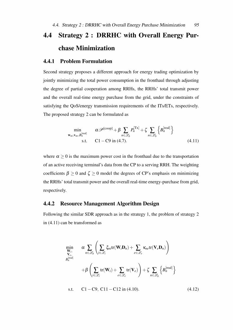
4.4. Strategy 2 : DRRHC with Overall Energy Purchase Minimization 95
4.4 Strategy 2 : DRRHC with Overall Energy Pur-
chase Minimization
4.4.1 Problem Formulation
Second strategy proposes a different approach for energy trading optimization by
jointly minimizing the total power consumption in the fronthaul through adjusting
the degree of partial cooperation among RRHs, the RRHs’ total transmit power
and the overall real-time energy purchase from the grid, under the constraints of
satisfying the QoS/energy transmission requirements of the ITs/ETs, respectively.
The proposed strategy 2 can be formulated as
minwni,vne,B
[real]n
αP [coop] +β ∑n∈Lb
P[Tx]n +ζ ∑
n∈Lb
{B[real]
n
}s.t. C1−C9 in (4.7). (4.11)
where α ≥ 0 is the maximum power cost in the fronthaul due to the transportation
of an active receiving terminal’s data from the CP to a serving RRH. The weighting
coefficients β ≥ 0 and ζ ≥ 0 model the degrees of CP’s emphasis on minimizing
the RRHs’ total transmit power and the overall real-time energy-purchase from grid,
respectively.
4.4.2 Resource Management Algorithm Design
Following the similar SDR approach as in the strategy 1, the problem of strategy 2
in (4.11) can be transformed as
minWi,Ve,
B[real]n
α ∑n∈Lb
(∑
i∈Li
ξnitr(WiDn)+ ∑e∈Le
κnetr(VeDn)
)
+β
(∑
i∈Li
tr(Wi)+ ∑e∈Le
tr(Ve)
)+ζ ∑
n∈Lb
{B[real]
n
}
s.t. C1−C9, C11−C12 in (4.10). (4.12)
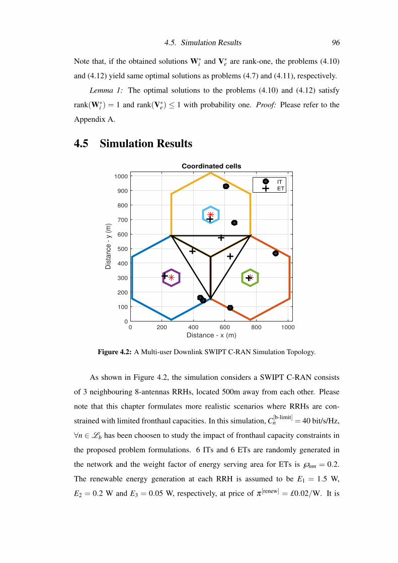
4.5. Simulation Results 96
Note that, if the obtained solutions W∗i and V∗e are rank-one, the problems (4.10)
and (4.12) yield same optimal solutions as problems (4.7) and (4.11), respectively.
Lemma 1: The optimal solutions to the problems (4.10) and (4.12) satisfy
rank(W∗i ) = 1 and rank(V∗e) ≤ 1 with probability one. Proof: Please refer to the
Appendix A.
4.5 Simulation Results
Distance - x (m)
0 200 400 600 800 1000
Dis
tan
ce -
y (
m)
0
100
200
300
400
500
600
700
800
900
1000
Coordinated cells
IT
ET
Figure 4.2: A Multi-user Downlink SWIPT C-RAN Simulation Topology.
As shown in Figure 4.2, the simulation considers a SWIPT C-RAN consists
of 3 neighbouring 8-antennas RRHs, located 500m away from each other. Please
note that this chapter formulates more realistic scenarios where RRHs are con-
strained with limited fronthaul capacities. In this simulation, C[b-limit]n = 40 bit/s/Hz,
∀n ∈Lb has been choosen to study the impact of fronthaul capacity constraints in
the proposed problem formulations. 6 ITs and 6 ETs are randomly generated in
the network and the weight factor of energy serving area for ETs is ℘nm = 0.2.
The renewable energy generation at each RRH is assumed to be E1 = 1.5 W,
E2 = 0.2 W and E3 = 0.05 W, respectively, at price of π [renew] = £0.02/W. It is
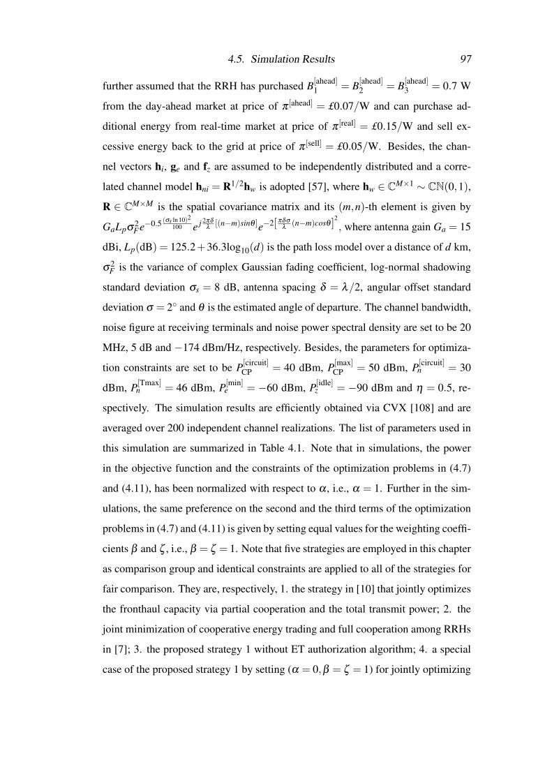
4.5. Simulation Results 97
further assumed that the RRH has purchased B[ahead]1 = B[ahead]
2 = B[ahead]3 = 0.7 W
from the day-ahead market at price of π [ahead] = £0.07/W and can purchase ad-
ditional energy from real-time market at price of π [real] = £0.15/W and sell ex-
cessive energy back to the grid at price of π [sell] = £0.05/W. Besides, the chan-
nel vectors hi, ge and fz are assumed to be independently distributed and a corre-
lated channel model hni = R1/2hw is adopted [57], where hw ∈ CM×1 ∼ CN(0,1),
R ∈ CM×M is the spatial covariance matrix and its (m,n)-th element is given by
GaLpσ2Fe−0.5 (σs ln10)2
100 e j 2πδ
λ[(n−m)sinθ ]e−2[ πδσ
λ(n−m)cosθ ]
2
, where antenna gain Ga = 15
dBi, Lp(dB) = 125.2+36.3log10(d) is the path loss model over a distance of d km,
σ2F is the variance of complex Gaussian fading coefficient, log-normal shadowing
standard deviation σs = 8 dB, antenna spacing δ = λ/2, angular offset standard
deviation σ = 2◦ and θ is the estimated angle of departure. The channel bandwidth,
noise figure at receiving terminals and noise power spectral density are set to be 20
MHz, 5 dB and −174 dBm/Hz, respectively. Besides, the parameters for optimiza-
tion constraints are set to be P[circuit]CP = 40 dBm, P[max]
CP = 50 dBm, P[circuit]n = 30
dBm, P[Tmax]n = 46 dBm, P[min]
e = −60 dBm, P[idle]z = −90 dBm and η = 0.5, re-
spectively. The simulation results are efficiently obtained via CVX [108] and are
averaged over 200 independent channel realizations. The list of parameters used in
this simulation are summarized in Table 4.1. Note that in simulations, the power
in the objective function and the constraints of the optimization problems in (4.7)
and (4.11), has been normalized with respect to α , i.e., α = 1. Further in the sim-
ulations, the same preference on the second and the third terms of the optimization
problems in (4.7) and (4.11) is given by setting equal values for the weighting coeffi-
cients β and ζ , i.e., β = ζ = 1. Note that five strategies are employed in this chapter
as comparison group and identical constraints are applied to all of the strategies for
fair comparison. They are, respectively, 1. the strategy in [10] that jointly optimizes
the fronthaul capacity via partial cooperation and the total transmit power; 2. the
joint minimization of cooperative energy trading and full cooperation among RRHs
in [7]; 3. the proposed strategy 1 without ET authorization algorithm; 4. a special
case of the proposed strategy 1 by setting (α = 0,β = ζ = 1) for jointly optimizing
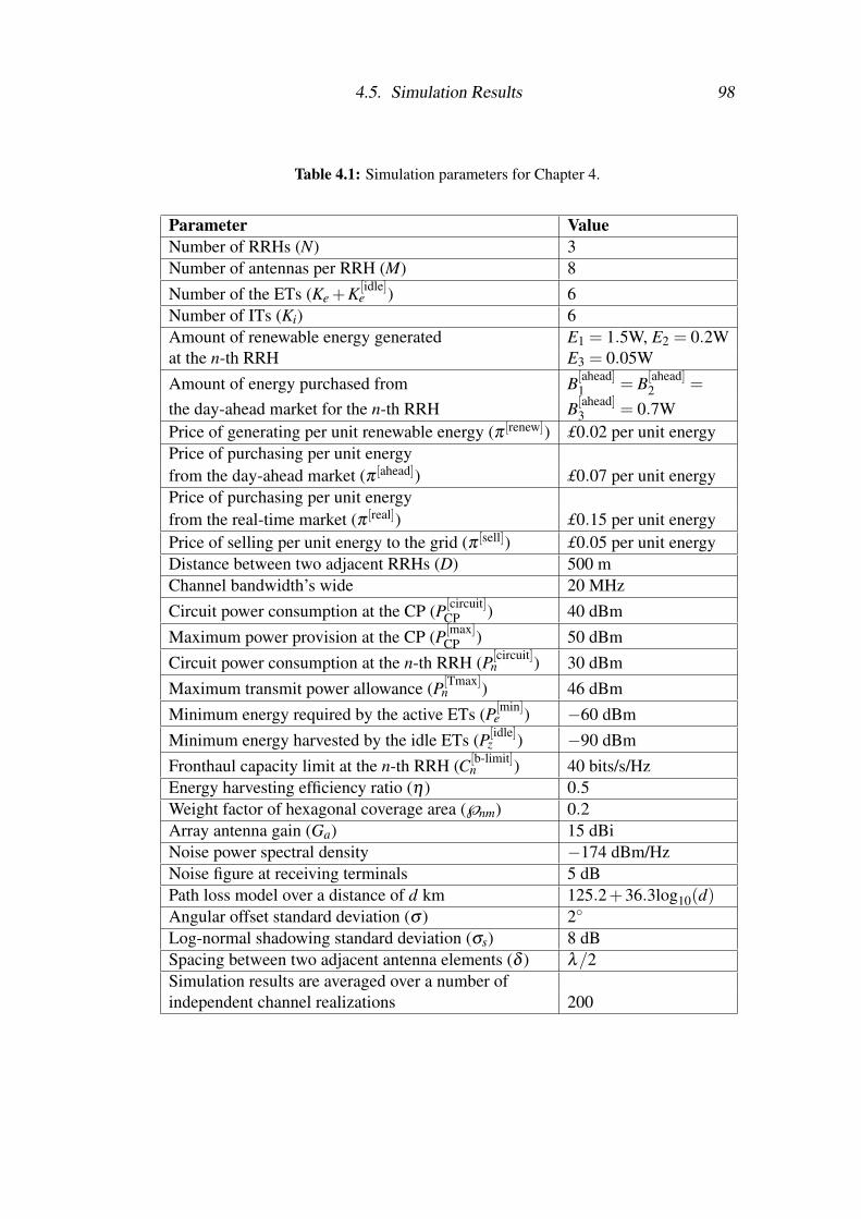
4.5. Simulation Results 98
Table 4.1: Simulation parameters for Chapter 4.
Parameter ValueNumber of RRHs (N) 3Number of antennas per RRH (M) 8Number of the ETs (Ke +K[idle]
e ) 6Number of ITs (Ki) 6Amount of renewable energy generated E1 = 1.5W, E2 = 0.2Wat the n-th RRH E3 = 0.05WAmount of energy purchased from B[ahead]
1 = B[ahead]2 =
the day-ahead market for the n-th RRH B[ahead]3 = 0.7W
Price of generating per unit renewable energy (π [renew]) £0.02 per unit energyPrice of purchasing per unit energyfrom the day-ahead market (π [ahead]) £0.07 per unit energyPrice of purchasing per unit energyfrom the real-time market (π [real]) £0.15 per unit energyPrice of selling per unit energy to the grid (π [sell]) £0.05 per unit energyDistance between two adjacent RRHs (D) 500 mChannel bandwidth’s wide 20 MHzCircuit power consumption at the CP (P[circuit]
CP ) 40 dBmMaximum power provision at the CP (P[max]
CP ) 50 dBmCircuit power consumption at the n-th RRH (P[circuit]
n ) 30 dBmMaximum transmit power allowance (P[Tmax]
n ) 46 dBmMinimum energy required by the active ETs (P[min]
e ) −60 dBmMinimum energy harvested by the idle ETs (P[idle]
z ) −90 dBmFronthaul capacity limit at the n-th RRH (C[b-limit]
n ) 40 bits/s/HzEnergy harvesting efficiency ratio (η) 0.5Weight factor of hexagonal coverage area (℘nm) 0.2Array antenna gain (Ga) 15 dBiNoise power spectral density −174 dBm/HzNoise figure at receiving terminals 5 dBPath loss model over a distance of d km 125.2+36.3log10(d)Angular offset standard deviation (σ ) 2◦
Log-normal shadowing standard deviation (σs) 8 dBSpacing between two adjacent antenna elements (δ ) λ/2Simulation results are averaged over a number ofindependent channel realizations 200
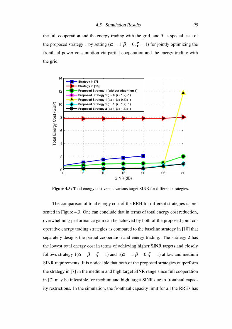
4.5. Simulation Results 99
the full cooperation and the energy trading with the grid, and 5. a special case of
the proposed strategy 1 by setting (α = 1,β = 0,ζ = 1) for jointly optimizing the
fronthaul power consumption via partial cooperation and the energy trading with
the grid.
0 5 10 15 20 25 300
2
4
6
8
10
12
14
SINR(dB)
Tota
l E
nerg
y C
ost (G
BP
)
Strategy in [7]
Strategy in [10]
Proposed Strategy 1 (without Algorithm 1)
Proposed Strategy 1 (α= 0, β = 1, ζ =1)
Proposed Strategy 1 (α= 1, β = 0, ζ =1)
Proposed Strategy 1 (α= 1, β = 1, ζ =1)
Proposed Strategy 2 (α= 1, β = 1, ζ =1)
Figure 4.3: Total energy cost versus various target SINR for different strategies.
The comparison of total energy cost of the RRH for different strategies is pre-
sented in Figure 4.3. One can conclude that in terms of total energy cost reduction,
overwhelming performance gain can be achieved by both of the proposed joint co-
operative energy trading strategies as compared to the baseline strategy in [10] that
separately designs the partial cooperation and energy trading. The strategy 2 has
the lowest total energy cost in terms of achieving higher SINR targets and closely
follows strategy 1(α = β = ζ = 1) and 1(α = 1,β = 0,ζ = 1) at low and medium
SINR requirements. It is noticeable that both of the proposed strategies outperform
the strategy in [7] in the medium and high target SINR range since full cooperation
in [7] may be infeasible for medium and high target SINR due to fronthaul capac-
ity restrictions. In the simulation, the fronthaul capacity limit for all the RRHs has
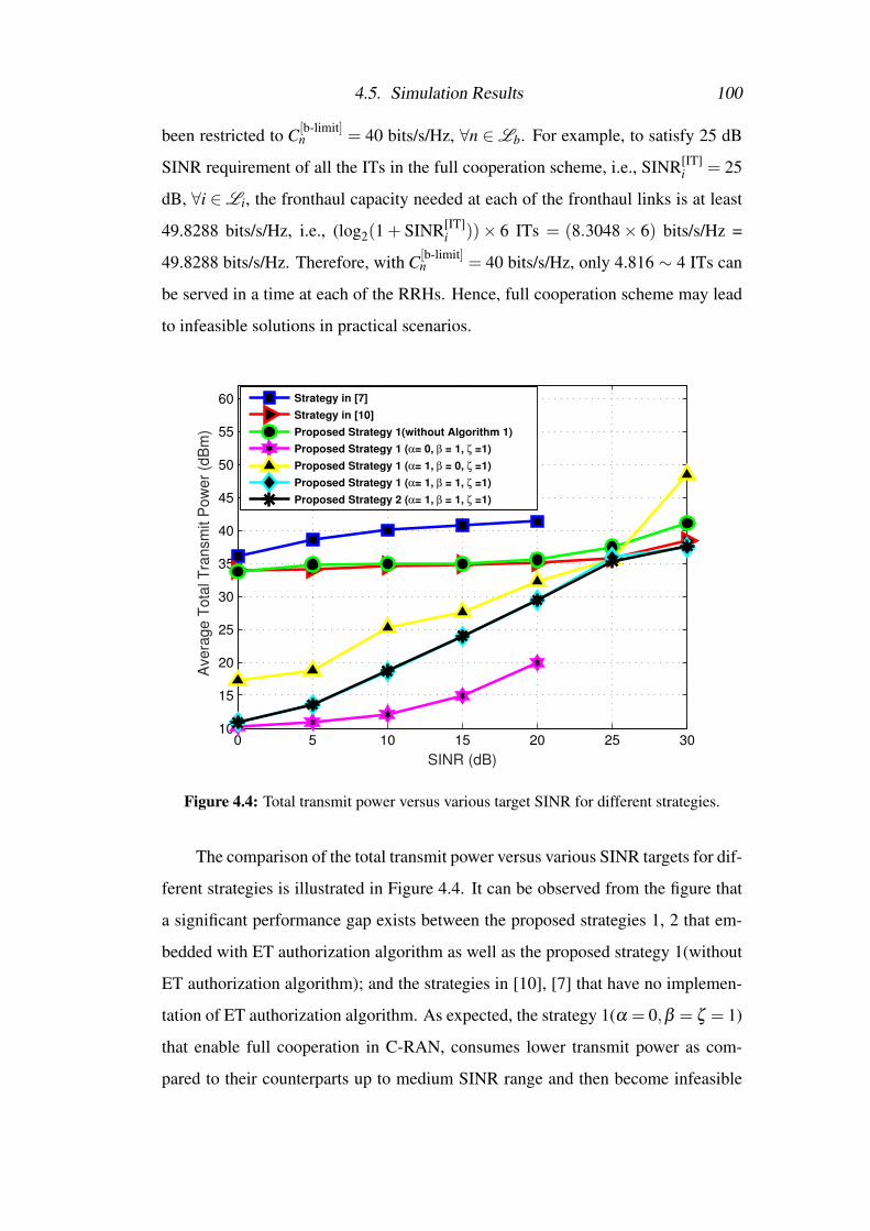
4.5. Simulation Results 100
been restricted to C[b-limit]n = 40 bits/s/Hz, ∀n ∈Lb. For example, to satisfy 25 dB
SINR requirement of all the ITs in the full cooperation scheme, i.e., SINR[IT]i = 25
dB, ∀i ∈Li, the fronthaul capacity needed at each of the fronthaul links is at least
49.8288 bits/s/Hz, i.e., (log2(1 + SINR[IT]i ))× 6 ITs = (8.3048× 6) bits/s/Hz =
49.8288 bits/s/Hz. Therefore, with C[b-limit]n = 40 bits/s/Hz, only 4.816 ∼ 4 ITs can
be served in a time at each of the RRHs. Hence, full cooperation scheme may lead
to infeasible solutions in practical scenarios.
0 5 10 15 20 25 3010
15
20
25
30
35
40
45
50
55
60
SINR (dB)
Avera
ge T
ota
l T
ransm
it P
ow
er
(dB
m)
Strategy in [7]
Strategy in [10]
Proposed Strategy 1(without Algorithm 1)
Proposed Strategy 1 (α= 0, β = 1, ζ =1)
Proposed Strategy 1 (α= 1, β = 0, ζ =1)
Proposed Strategy 1 (α= 1, β = 1, ζ =1)
Proposed Strategy 2 (α= 1, β = 1, ζ =1)
Figure 4.4: Total transmit power versus various target SINR for different strategies.
The comparison of the total transmit power versus various SINR targets for dif-
ferent strategies is illustrated in Figure 4.4. It can be observed from the figure that
a significant performance gap exists between the proposed strategies 1, 2 that em-
bedded with ET authorization algorithm as well as the proposed strategy 1(without
ET authorization algorithm); and the strategies in [10], [7] that have no implemen-
tation of ET authorization algorithm. As expected, the strategy 1(α = 0,β = ζ = 1)
that enable full cooperation in C-RAN, consumes lower transmit power as com-
pared to their counterparts up to medium SINR range and then become infeasible
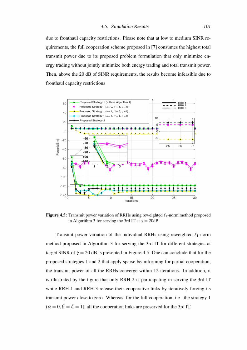
4.5. Simulation Results 101
due to fronthaul capacity restrictions. Please note that at low to medium SINR re-
quirements, the full cooperation scheme proposed in [7] consumes the highest total
transmit power due to its proposed problem formulation that only minimize en-
ergy trading without jointly minimize both energy trading and total transmit power.
Then, above the 20 dB of SINR requirements, the results become infeasible due to
fronthaul capacity restrictions
Iterations0 5 10 15 20 25 30
Pow
er(
dB
m)
-140
-120
-100
-80
-60
-40
-20
0
20
40
60Proposed Strategy 1 (without Algorithm 1)
Proposed Strategy 1 (α= 0, β = 1, ζ =1)
Proposed Strategy 1 (α= 1, β = 0, ζ =1)
Proposed Strategy 1 (α= 1, β = 1, ζ =1)
Proposed Strategy 2
25 26 27
-5
0
5
10
1 2 3
-110
-100
-90
-80
-70
-60
RRH 1RRH 2RRH 3
Figure 4.5: Transmit power variation of RRHs using reweighted `1-norm method proposedin Algorithm 3 for serving the 3rd IT at γ = 20dB.
Transmit power variation of the individual RRHs using reweighted `1-norm
method proposed in Algorithm 3 for serving the 3rd IT for different strategies at
target SINR of γ = 20 dB is presented in Figure 4.5. One can conclude that for the
proposed strategies 1 and 2 that apply sparse beamforming for partial cooperation,
the transmit power of all the RRHs converge within 12 iterations. In addition, it
is illustrated by the figure that only RRH 2 is participating in serving the 3rd IT
while RRH 1 and RRH 3 release their cooperative links by iteratively forcing its
transmit power close to zero. Whereas, for the full cooperation, i.e., the strategy 1
(α = 0,β = ζ = 1), all the cooperation links are preserved for the 3rd IT.
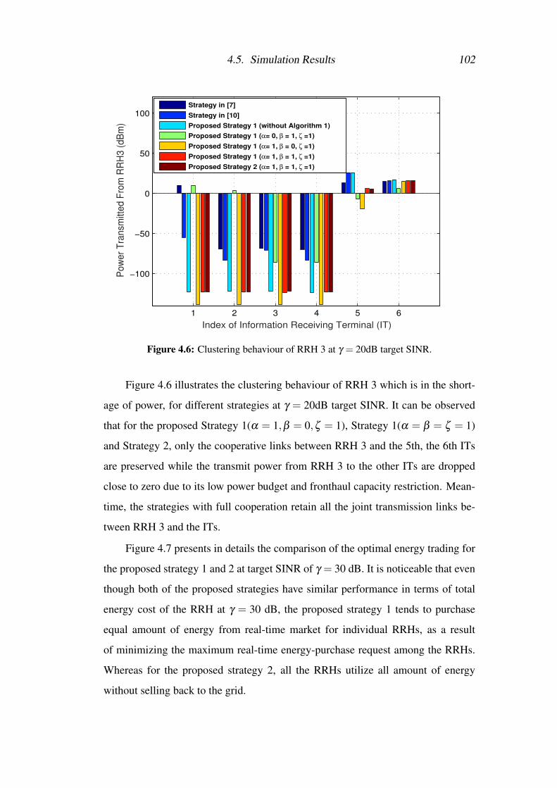
4.5. Simulation Results 102
1 2 3 4 5 6
−100
−50
0
50
100
Index of Information Receiving Terminal (IT)
Pow
er
Tra
nsm
itted F
rom
RR
H3 (
dB
m)
Strategy in [7]
Strategy in [10]
Proposed Strategy 1 (without Algorithm 1)
Proposed Strategy 1 (α= 0, β = 1, ζ =1)
Proposed Strategy 1 (α= 1, β = 0, ζ =1)
Proposed Strategy 1 (α= 1, β = 1, ζ =1)
Proposed Strategy 2 (α= 1, β = 1, ζ =1)
Figure 4.6: Clustering behaviour of RRH 3 at γ = 20dB target SINR.
Figure 4.6 illustrates the clustering behaviour of RRH 3 which is in the short-
age of power, for different strategies at γ = 20dB target SINR. It can be observed
that for the proposed Strategy 1(α = 1,β = 0,ζ = 1), Strategy 1(α = β = ζ = 1)
and Strategy 2, only the cooperative links between RRH 3 and the 5th, the 6th ITs
are preserved while the transmit power from RRH 3 to the other ITs are dropped
close to zero due to its low power budget and fronthaul capacity restriction. Mean-
time, the strategies with full cooperation retain all the joint transmission links be-
tween RRH 3 and the ITs.
Figure 4.7 presents in details the comparison of the optimal energy trading for
the proposed strategy 1 and 2 at target SINR of γ = 30 dB. It is noticeable that even
though both of the proposed strategies have similar performance in terms of total
energy cost of the RRH at γ = 30 dB, the proposed strategy 1 tends to purchase
equal amount of energy from real-time market for individual RRHs, as a result
of minimizing the maximum real-time energy-purchase request among the RRHs.
Whereas for the proposed strategy 2, all the RRHs utilize all amount of energy
without selling back to the grid.
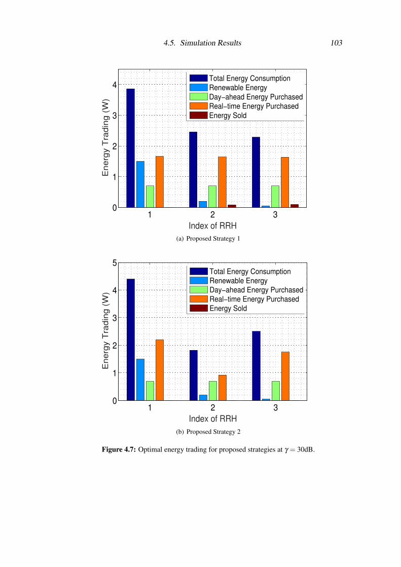
4.5. Simulation Results 103
1 2 30
1
2
3
4
Index of RRH
En
erg
y T
rad
ing
(W
)
Total Energy Consumption
Renewable Energy
Day−ahead Energy Purchased
Real−time Energy Purchased
Energy Sold
(a) Proposed Strategy 1
1 2 30
1
2
3
4
5
Index of RRH
En
erg
y T
rad
ing
(W
)
Total Energy Consumption
Renewable Energy
Day−ahead Energy Purchased
Real−time Energy Purchased
Energy Sold
(b) Proposed Strategy 2
Figure 4.7: Optimal energy trading for proposed strategies at γ = 30dB.
4.6. Concluding Remarks 104
4.6 Concluding RemarksThis chapter proposes two joint real-time resource management and energy trad-
ing strategies based on sparse beamforming technique in downlink green C-RAN
with SWIPT, taking into account the individual fronthaul capacity restrictions, to
strike an optimum balance between the total power consumption in the fronthaul
through adjusting the degree of partial cooperation among RRHs, RRHs’ total trans-
mit power and their maximum or overall energy purchased from the real-time mar-
ket. To further improve the energy efficiency, an iterative ET authorization algo-
rithm is proposed to design energy beamformers only for the ETs located within the
energy serving area of RRHs. By employing the reweighted `1-norm approximation
for `0-norm and SDR, the solution sparsity to the original non-convex optimization
problems in (4.7) and (4.11) can be obtained. Simulation results confirm that both
of the proposed strategies outperform two other recently proposed schemes in terms
of improving the energy efficiency and reducing total energy cost of the RRH in a
realistic C-RAN scenario.
Chapter 5
Combinatorial Multi-Armed Bandit
Approach for Proactive Energy
Management in Green C-RAN
5.1 IntroductionThis chapter further extends the previous works to a learning-based practical ap-
proach and assume that the centralized cloud computing processor (CP) has no ini-
tial knowledge of forthcoming power budget and energy consumption at the individ-
ual remote radio heads (RRHs). Two novel iterative algorithms based on combina-
torial multi-armed bandit (CMAB) approach, namely, Forward CMAB (ForCMAB)
energy trading and Reverse CMAB (RevCMAB) energy trading are introduced to
search for the optimal set of energy packages in ascending and descending order
of package sizes, respectively. The aim of the proposed strategies is to find the set
of optimal sizes of the energy packages to be purchased from the day-ahead mar-
ket by observing the instantaneous energy demand and learning from the behaviour
of cooperative energy trading, so that the total cost of the network operator can be
minimized.
5.1.1 Organization
This chapter follows the same system model and problem formulation that have
been proposed for Strategy 2 : Dynamic RRH-centric Clustering (DRRHC) with

5.2. DRRHC with Overall Energy Purchase Minimization 106
Overall Energy Purchase Minimization in section 4.4, Chapter 4. For the conve-
nience of reader, the reweighted `1-norm method for simultaneous wireless informa-
tion and power transfer (SWIPT) algorithm proposed in Algorithm 3 and the Strat-
egy 2 that has been transformed in numerically tractable form proposed in problem
(4.12), both from Chapter 4, are attached in section 5.2 in this chapter. Two CMAB
strategies: Forward Combinatorial Multi-Armed Bandit and Reverse Combinatorial
Multi-Armed Bandit are proposed in section 5.4 and 5.5, respectively. Numerical
simulation results are analyzed in section 5.6. Finally, section 5.7 summarizes this
chapter.
5.2 DRRHC with Overall Energy Purchase Mini-
mization
The reweighted `1-norm method for SWIPT for sparse beamforming technique that
has been developed in Algorithm 3 and the proposed Strategy 2 that has been trans-
formed in numerically tractable form in problem (4.12), Chapter 4, are represented
as follows, respectively,
Algorithm 4 Reweighted `1-norm method for SWIPT
1: Initialize: constant µ → 0, iteration count t = 0, weighting factor ξni(t) = 1,κne(t) = 1, maximum number of iterations tmax, Ri(t) = log2(1+ γi).
2: while ξni and κne are not converged or t 6= tmax do3: Find the optimal beamformers W∗i (t) and V∗e(t) by solving (5.1);4: Update the weight factor ξni(t +1) as follows,
ξni(t +1) = 1tr(W∗i (t)Dn)+µ
, ∀n ∈Lb, i ∈Li;5: Update the weight factor κne(t +1) as follows,
κne(t +1) = 1tr(V∗e(t)Dn)+µ
, ∀n ∈Lb,e ∈Le;6: Calculate the achievable rate Ri(t) as follows,
Ri(t) = log2[1+tr(HiW∗i (t))
∑j∈Li, j 6=i
tr(HiW∗j(t))+ ∑e∈Le
tr(HiV∗e(t))+σ2i];
7: Update Ri(t +1) = Ri(t);8: Increment the iteration number t = t +1;9: end while.
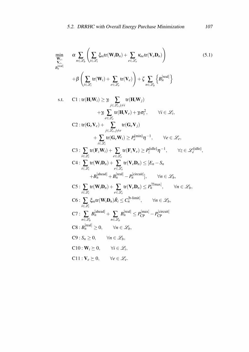
5.2. DRRHC with Overall Energy Purchase Minimization 107
minWi,Ve,
B[real]n
α ∑n∈Lb
(∑
i∈Li
ξnitr(WiDn)+ ∑e∈Le
κnetr(VeDn)
)(5.1)
+β
(∑
i∈Li
tr(Wi)+ ∑e∈Le
tr(Ve)
)+ζ ∑
n∈Lb
{B[real]
n
}
s.t. C1 : tr(HiWi)≥ γi ∑j∈Li, j 6=i
tr(HiW j)
+γi ∑e∈Le
tr(HiVe)+ γiσ2i , ∀i ∈Li,
C2 : tr(GeVe)+ ∑j∈Le, j 6=e
tr(GeV j)
+ ∑i∈Li
tr(GeWi)≥ P[min]e η
−1, ∀e ∈Le,
C3 : ∑i∈Li
tr(FzWi)+ ∑e∈Le
tr(FzVe)≥ P[idle]z η
−1, ∀z ∈L [idle]e ,
C4 : ∑i∈Li
tr(WiDn)+ ∑e∈Le
tr(VeDn)≤ [En−Sn
+B[ahead]n +B[real]
n −P[circuit]n ], ∀n ∈Lb,
C5 : ∑i∈Li
tr(WiDn)+ ∑e∈Le
tr(VeDn)≤ P[Tmax]n , ∀n ∈Lb,
C6 : ∑i∈Li
ξnitr(WiDn)Ri ≤C[b-limit]n , ∀n ∈Lb,
C7 : ∑n∈Lb
B[ahead]n + ∑
n∈Lb
B[real]n ≤ P[max]
CP −P[circuit]CP
C8 : B[real]n ≥ 0, ∀n ∈Lb,
C9 : Sn ≥ 0, ∀n ∈Lb,
C10 : Wi � 0, ∀i ∈Li,
C11 : Ve � 0, ∀e ∈Le.
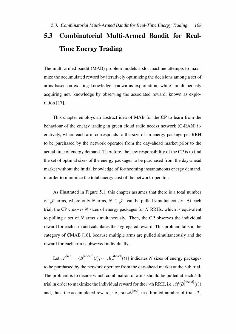
5.3. Combinatorial Multi-Armed Bandit for Real-Time Energy Trading 108
5.3 Combinatorial Multi-Armed Bandit for Real-
Time Energy Trading
The multi-armed bandit (MAB) problem models a slot machine attempts to maxi-
mize the accumulated reward by iteratively optimizing the decisions among a set of
arms based on existing knowledge, known as exploitation, while simultaneously
acquiring new knowledge by observing the associated reward, known as explo-
ration [17].
This chapter employs an abstract idea of MAB for the CP to learn from the
behaviour of the energy trading in green cloud radio access network (C-RAN) it-
eratively, where each arm corresponds to the size of an energy package per RRH
to be purchased by the network operator from the day-ahead market prior to the
actual time of energy demand. Therefore, the new responsibility of the CP is to find
the set of optimal sizes of the energy packages to be purchased from the day-ahead
market without the initial knowledge of forthcoming instantaneous energy demand,
in order to minimize the total energy cost of the network operator.
As illustrated in Figure 5.1, this chapter assumes that there is a total number
of J arms, where only N arms, N ⊂J , can be pulled simultaneously. At each
trial, the CP chooses N sizes of energy packages for N RRHs, which is equivalent
to pulling a set of N arms simultaneously. Then, the CP observes the individual
reward for each arm and calculates the aggregated reward. This problem falls in the
category of CMAB [16], because multiple arms are pulled simultaneously and the
reward for each arm is observed individually.
Let A[set]
t = {B[ahead]1 (t), · · · ,B[ahead]
N (t)} indicates N sizes of energy packages
to be purchased by the network operator from the day-ahead market at the t-th trial.
The problem is to decide which combination of arms should be pulled at each t-th
trial in order to maximize the individual reward for the n-th RRH, i.e., R(B[ahead]n (t))
and, thus, the accumulated reward, i.e., R(A[set]
t ) in a limited number of trials T ,
5.3. Combinatorial Multi-Armed Bandit for Real-Time Energy Trading 109
Central Processor (CP)
Smart Meter
Two-way power flow Grid-deployed communication/!control links
RRH_1
ET
IT
IT
ITIT
IT
ITET ET
idle ET idle ET
Renewable energy !harvesting devices
Smart Meter Smart Meter
Reward_1Reward_2 Reward_N
!N arms, N ⊂ J , can be pulled simultaneously
RRH_2 RRH_N
. . .
. . .
. . .arm_1 arm_2 arm_J
Figure 5.1: Combinatorial MAB problem for the proposed resource management and en-ergy trading in green C-RAN.
which can be calculated as
R(B[ahead]n (t)) = B[total]
n (0)−B[total]n (t), ∀n ∈Lb, (5.2)
R(A[set]
t ) = ∑n∈Lb
R(B[ahead]n (t)). (5.3)
B[total]n (0) and B[total]
n (t) in (5.2) are the total energy cost of the network operator con-
sumed by the n-th RRH at the initial trial, i.e., t = 0 and at the t-th trial respectively,
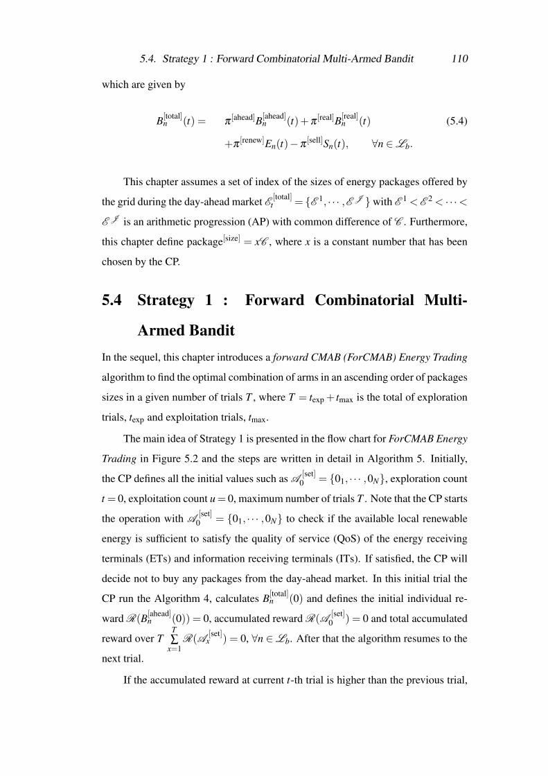
5.4. Strategy 1 : Forward Combinatorial Multi-Armed Bandit 110
which are given by
B[total]n (t) = π
[ahead]B[ahead]n (t)+π
[real]B[real]n (t) (5.4)
+π[renew]En(t)−π
[sell]Sn(t), ∀n ∈Lb.
This chapter assumes a set of index of the sizes of energy packages offered by
the grid during the day-ahead market E[total]
t = {E 1, · · · ,E J }with E 1 < E 2 < · · ·<E J is an arithmetic progression (AP) with common difference of C . Furthermore,
this chapter define package[size] = xC , where x is a constant number that has been
chosen by the CP.
5.4 Strategy 1 : Forward Combinatorial Multi-
Armed BanditIn the sequel, this chapter introduces a forward CMAB (ForCMAB) Energy Trading
algorithm to find the optimal combination of arms in an ascending order of packages
sizes in a given number of trials T , where T = texp + tmax is the total of exploration
trials, texp and exploitation trials, tmax.
The main idea of Strategy 1 is presented in the flow chart for ForCMAB Energy
Trading in Figure 5.2 and the steps are written in detail in Algorithm 5. Initially,
the CP defines all the initial values such as A[set]
0 = {01, · · · ,0N}, exploration count
t = 0, exploitation count u= 0, maximum number of trials T . Note that the CP starts
the operation with A[set]
0 = {01, · · · ,0N} to check if the available local renewable
energy is sufficient to satisfy the quality of service (QoS) of the energy receiving
terminals (ETs) and information receiving terminals (ITs). If satisfied, the CP will
decide not to buy any packages from the day-ahead market. In this initial trial the
CP run the Algorithm 4, calculates B[total]n (0) and defines the initial individual re-
ward R(B[ahead]n (0)) = 0, accumulated reward R(A
[set]0 ) = 0 and total accumulated
reward over TT∑
x=1R(A
[set]x ) = 0, ∀n ∈Lb. After that the algorithm resumes to the
next trial.
If the accumulated reward at current t-th trial is higher than the previous trial,
5.4. Strategy 1 : Forward Combinatorial Multi-Armed Bandit 111
i.e., R(A[set]
t ) ≥ R(A[set]
t−1 ), the algorithm proceeds to the exploration stage. In
the exploration stage, if the individual reward for the n-th RRH at the current trial is
also higher than the previous trial, i.e., R(B[ahead]n (t))≥R(B[ahead]
n (t−1)),∀n∈Lb,
then the algorithm explores a new combinatorial arms by purchasing higher sizes
of energy packages from the day-ahead market. Perhaps this new combinatorial
of arms can contribute to a higher accumulated reward than previous trial. On the
other hand, if the accumulated reward at the current t-th trial is lower than the
previous trial, i.e., R(A[set]
t )≤R(A[set]
t−1 ), the algorithm stops the exploration stage
and decides to purchase the optimal combination of arms in the exploitation stage
until the given number of T trials end. In other words, at each trial t, the CP decides
to purchase N combination of sizes of the energy packages from the day-ahead
market for N RRHs based on the individual reward obtained from the current trial t
and the previous trial (t−1) and the iterations of CMAB search are continued until
the aggregated reward is maximized.
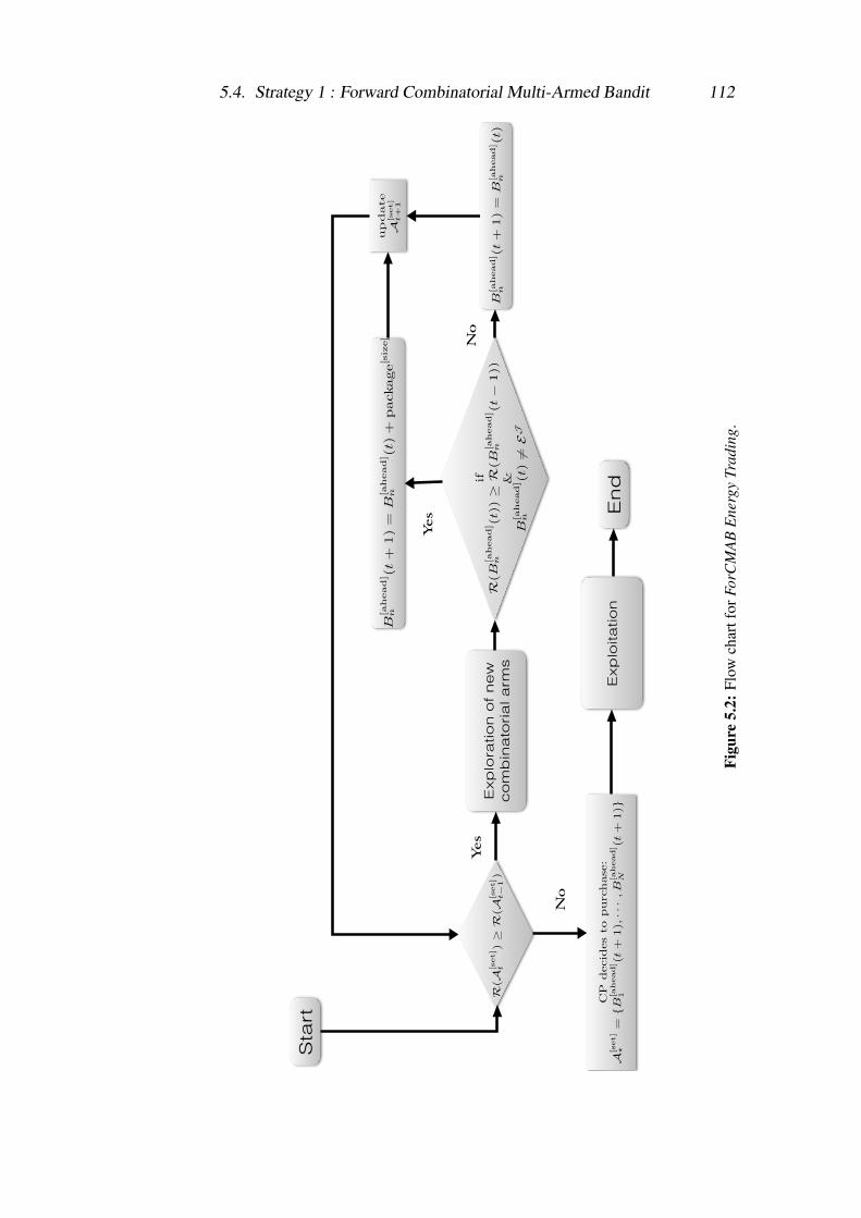
5.4. Strategy 1 : Forward Combinatorial Multi-Armed Bandit 112
R(A
[set]
t)�
R(A
[set]
t�
1)
Exp
lora
tion o
f new
com
bin
ato
rial a
rms
ifR
(B
[ahead]
n(t)
)�
R(B
[ahead]
n(t�
1))
&B
[ahead]
n(t)
6=E
J
B[a
head]
n(t+
1)
=B
[ahead]
n(t)
+package[s
ize],
B[a
head]
n(t+
1)
=B
[ahead]
n(t)
Yes
Yes
No
update
A[set]
t+
1
CP
decid
es
to
purchase:
A[s
et]
?=
{B[a
head]
1(t+
1),··
·,B
[ahead]
N(t+
1)}
Exp
loita
tion
No
Sta
rt
En
d
Figu
re5.
2:Fl
owch
artf
orFo
rCM
AB
Ene
rgy
Trad
ing.
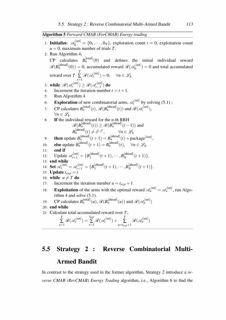
5.5. Strategy 2 : Reverse Combinatorial Multi-Armed Bandit 113
Algorithm 5 Forward CMAB (ForCMAB) Energy trading
1: Initialize: A[set]
0 = {01, · · · ,0N}, exploration count t = 0, exploitation countu = 0, maximum number of trials T .
2: Run Algorithm 4;CP calculates B[total]
n (0) and defines the initial individual rewardR(B[ahead]
n (0)) = 0, accumulated reward R(A[set]
0 ) = 0 and total accumulated
reward over TT∑
x=1R(A
[set]x ) = 0, ∀n ∈Lb
3: while R(A[set]
t )≥R(A[set]
t−1 ) do4: Increment the iteration number t = t +1.5: Run Algorithm 46: Exploration of new combinatorial arms, A
[set]t by solving (5.1) ;
7: CP calculates B[total]n (t), R(B[ahead]
n (t)) and R(A[set]
t ),∀n ∈Lb
8: If the individual reward for the n-th RRHR(B[ahead]
n (t))≥R(B[ahead]n (t−1)) and
B[ahead]n (t) 6= E J , ∀n ∈Lb
9: then update B[ahead]n (t +1) = B[ahead]
n (t)+package[size],10: else update B[ahead]
n (t +1) = B[ahead]n (t), ∀n ∈Lb.
11: end if12: Update A
[set]t+1 = {B[ahead]
1 (t +1), · · · ,B[ahead]N (t +1)}.
13: end while14: Set A
[set]? = A
[set]t+1 = {B[ahead]
1 (t +1), · · · ,B[ahead]N (t +1)}.
15: Update texp = t16: while u 6= T do17: Increment the iteration number u = texp +1.18: Exploitation of the arms with the optimal reward A
[set]u = A
[set]? , run Algo-
rithm 4 and solve (5.1).19: CP calculates B[total]
n (u), R(B[ahead]n (u)) and R(A
[set]u )
20: end while21: Calculate total accumulated reward over T ;
T∑
x=1R(A
[set]x ) =
texp
∑t=1
R(A[set]
t )+T∑
u=texp+1R(A
[set]u )
5.5 Strategy 2 : Reverse Combinatorial Multi-
Armed BanditIn contrast to the strategy used in the former algorithm, Strategy 2 introduce a re-
verse CMAB (RevCMAB) Energy Trading algorithm, i.e., Algorithm 6 to find the
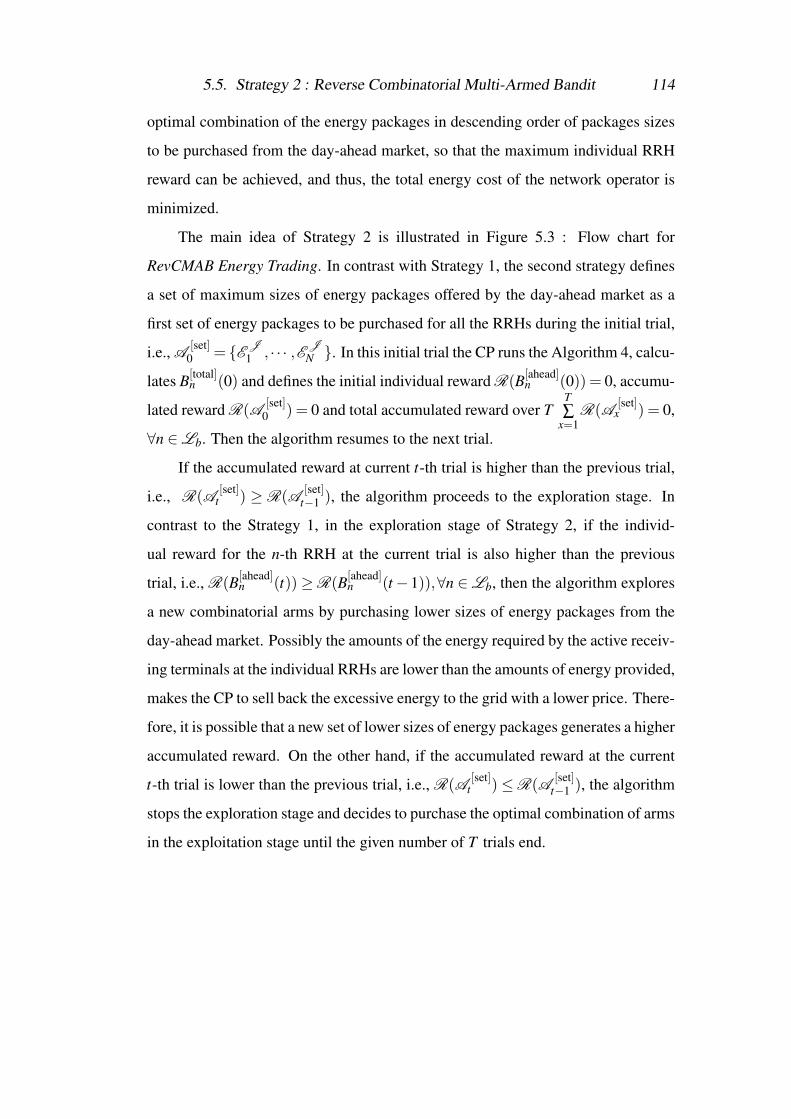
5.5. Strategy 2 : Reverse Combinatorial Multi-Armed Bandit 114
optimal combination of the energy packages in descending order of packages sizes
to be purchased from the day-ahead market, so that the maximum individual RRH
reward can be achieved, and thus, the total energy cost of the network operator is
minimized.
The main idea of Strategy 2 is illustrated in Figure 5.3 : Flow chart for
RevCMAB Energy Trading. In contrast with Strategy 1, the second strategy defines
a set of maximum sizes of energy packages offered by the day-ahead market as a
first set of energy packages to be purchased for all the RRHs during the initial trial,
i.e., A [set]0 = {E J
1 , · · · ,E JN }. In this initial trial the CP runs the Algorithm 4, calcu-
lates B[total]n (0) and defines the initial individual reward R(B[ahead]
n (0)) = 0, accumu-
lated reward R(A[set]
0 ) = 0 and total accumulated reward over TT∑
x=1R(A
[set]x ) = 0,
∀n ∈Lb. Then the algorithm resumes to the next trial.
If the accumulated reward at current t-th trial is higher than the previous trial,
i.e., R(A[set]
t ) ≥ R(A[set]
t−1 ), the algorithm proceeds to the exploration stage. In
contrast to the Strategy 1, in the exploration stage of Strategy 2, if the individ-
ual reward for the n-th RRH at the current trial is also higher than the previous
trial, i.e., R(B[ahead]n (t))≥R(B[ahead]
n (t−1)),∀n ∈Lb, then the algorithm explores
a new combinatorial arms by purchasing lower sizes of energy packages from the
day-ahead market. Possibly the amounts of the energy required by the active receiv-
ing terminals at the individual RRHs are lower than the amounts of energy provided,
makes the CP to sell back the excessive energy to the grid with a lower price. There-
fore, it is possible that a new set of lower sizes of energy packages generates a higher
accumulated reward. On the other hand, if the accumulated reward at the current
t-th trial is lower than the previous trial, i.e., R(A[set]
t )≤R(A[set]
t−1 ), the algorithm
stops the exploration stage and decides to purchase the optimal combination of arms
in the exploitation stage until the given number of T trials end.
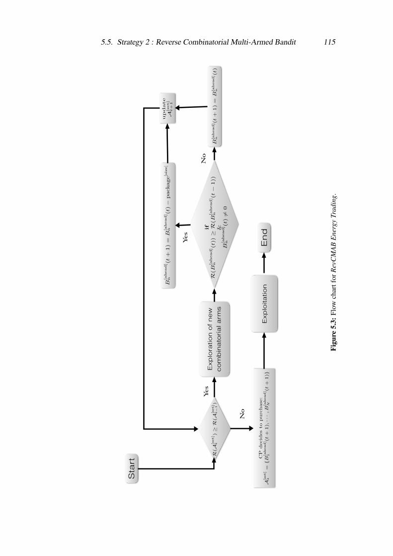
5.5. Strategy 2 : Reverse Combinatorial Multi-Armed Bandit 115
R(A
[set]
t)�
R(A
[set]
t�
1)
Exp
lora
tion o
f new
com
bin
ato
rial a
rms
B[a
head]
n(t
+1)
=B
[ahead]
n(t
)�
package[s
ize]
B[a
head]
n(t+
1)
=B
[ahead]
n(t)
Yes
Yes
No
update
A[set]
t+
1
CP
decid
es
to
purchase:
A[s
et]
?=
{B[a
head]
1(t+
1),··
·,B
[ahead]
N(t+
1)}
Exp
loita
tion
No
Sta
rt
En
difR
(B
[ahead]
n(t)
)�
R(B
[ahead]
n(t�
1))
&B
[ahead]
n(t)
6=0
Figu
re5.
3:Fl
owch
artf
orR
evC
MA
BE
nerg
yTr
adin
g.
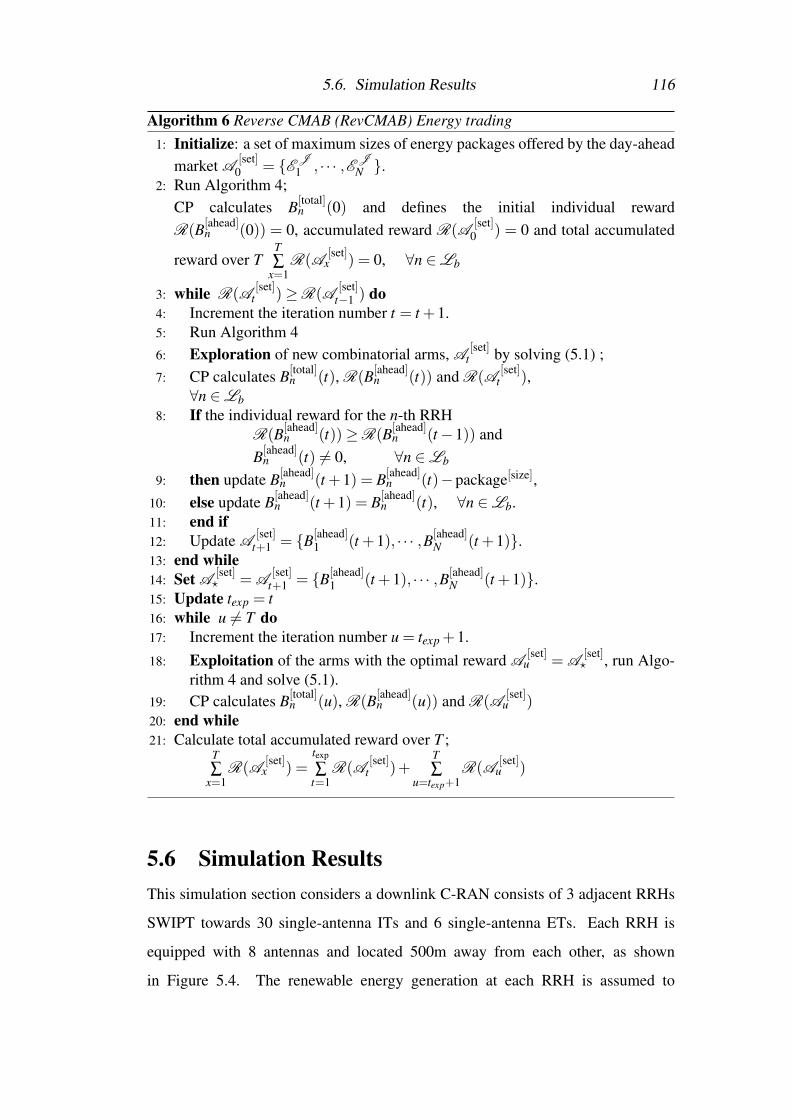
5.6. Simulation Results 116
Algorithm 6 Reverse CMAB (RevCMAB) Energy trading1: Initialize: a set of maximum sizes of energy packages offered by the day-ahead
market A[set]
0 = {E J1 , · · · ,E J
N }.2: Run Algorithm 4;
CP calculates B[total]n (0) and defines the initial individual reward
R(B[ahead]n (0)) = 0, accumulated reward R(A
[set]0 ) = 0 and total accumulated
reward over TT∑
x=1R(A
[set]x ) = 0, ∀n ∈Lb
3: while R(A[set]
t )≥R(A[set]
t−1 ) do4: Increment the iteration number t = t +1.5: Run Algorithm 46: Exploration of new combinatorial arms, A
[set]t by solving (5.1) ;
7: CP calculates B[total]n (t), R(B[ahead]
n (t)) and R(A[set]
t ),∀n ∈Lb
8: If the individual reward for the n-th RRHR(B[ahead]
n (t))≥R(B[ahead]n (t−1)) and
B[ahead]n (t) 6= 0, ∀n ∈Lb
9: then update B[ahead]n (t +1) = B[ahead]
n (t)−package[size],10: else update B[ahead]
n (t +1) = B[ahead]n (t), ∀n ∈Lb.
11: end if12: Update A
[set]t+1 = {B[ahead]
1 (t +1), · · · ,B[ahead]N (t +1)}.
13: end while14: Set A
[set]? = A
[set]t+1 = {B[ahead]
1 (t +1), · · · ,B[ahead]N (t +1)}.
15: Update texp = t16: while u 6= T do17: Increment the iteration number u = texp +1.18: Exploitation of the arms with the optimal reward A
[set]u = A
[set]? , run Algo-
rithm 4 and solve (5.1).19: CP calculates B[total]
n (u), R(B[ahead]n (u)) and R(A
[set]u )
20: end while21: Calculate total accumulated reward over T ;
T∑
x=1R(A
[set]x ) =
texp
∑t=1
R(A[set]
t )+T∑
u=texp+1R(A
[set]u )
5.6 Simulation ResultsThis simulation section considers a downlink C-RAN consists of 3 adjacent RRHs
SWIPT towards 30 single-antenna ITs and 6 single-antenna ETs. Each RRH is
equipped with 8 antennas and located 500m away from each other, as shown
in Figure 5.4. The renewable energy generation at each RRH is assumed to
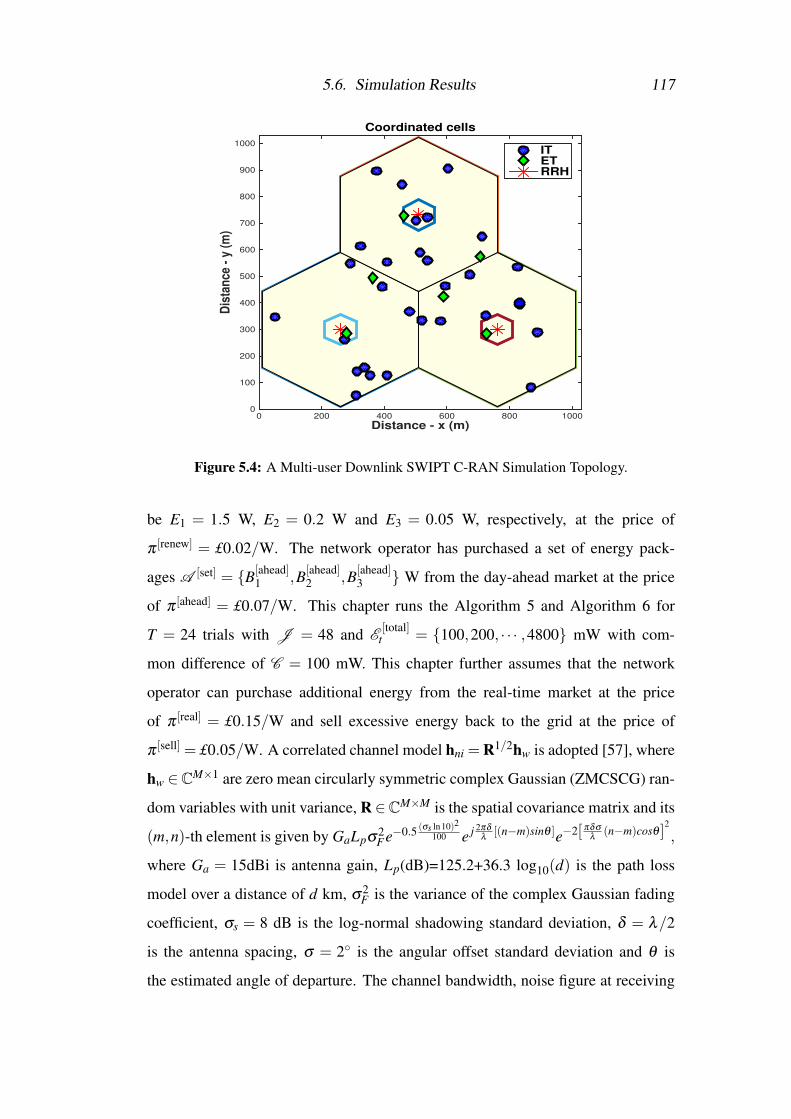
5.6. Simulation Results 117
Distance - x (m)0 200 400 600 800 1000
Dis
tan
ce -
y (
m)
0
100
200
300
400
500
600
700
800
900
1000
Coordinated cells
ITETRRH
Figure 5.4: A Multi-user Downlink SWIPT C-RAN Simulation Topology.
be E1 = 1.5 W, E2 = 0.2 W and E3 = 0.05 W, respectively, at the price of
π [renew] = £0.02/W. The network operator has purchased a set of energy pack-
ages A [set] = {B[ahead]1 ,B[ahead]
2 ,B[ahead]3 } W from the day-ahead market at the price
of π [ahead] = £0.07/W. This chapter runs the Algorithm 5 and Algorithm 6 for
T = 24 trials with J = 48 and E[total]
t = {100,200, · · · ,4800} mW with com-
mon difference of C = 100 mW. This chapter further assumes that the network
operator can purchase additional energy from the real-time market at the price
of π [real] = £0.15/W and sell excessive energy back to the grid at the price of
π [sell] = £0.05/W. A correlated channel model hni = R1/2hw is adopted [57], where
hw ∈CM×1 are zero mean circularly symmetric complex Gaussian (ZMCSCG) ran-
dom variables with unit variance, R∈CM×M is the spatial covariance matrix and its
(m,n)-th element is given by GaLpσ2Fe−0.5 (σs ln10)2
100 e j 2πδ
λ[(n−m)sinθ ]e−2[ πδσ
λ(n−m)cosθ ]
2
,
where Ga = 15dBi is antenna gain, Lp(dB)=125.2+36.3 log10(d) is the path loss
model over a distance of d km, σ2F is the variance of the complex Gaussian fading
coefficient, σs = 8 dB is the log-normal shadowing standard deviation, δ = λ/2
is the antenna spacing, σ = 2◦ is the angular offset standard deviation and θ is
the estimated angle of departure. The channel bandwidth, noise figure at receiving
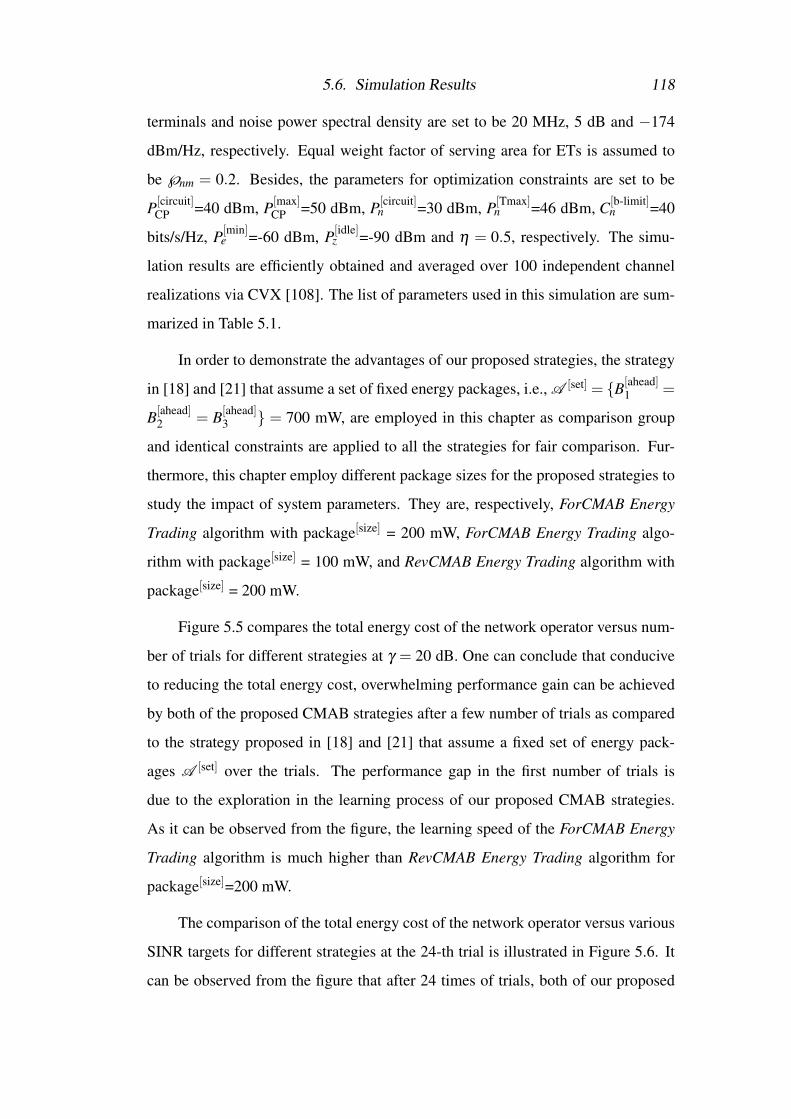
5.6. Simulation Results 118
terminals and noise power spectral density are set to be 20 MHz, 5 dB and −174
dBm/Hz, respectively. Equal weight factor of serving area for ETs is assumed to
be ℘nm = 0.2. Besides, the parameters for optimization constraints are set to be
P[circuit]CP =40 dBm, P[max]
CP =50 dBm, P[circuit]n =30 dBm, P[Tmax]
n =46 dBm, C[b-limit]n =40
bits/s/Hz, P[min]e =-60 dBm, P[idle]
z =-90 dBm and η = 0.5, respectively. The simu-
lation results are efficiently obtained and averaged over 100 independent channel
realizations via CVX [108]. The list of parameters used in this simulation are sum-
marized in Table 5.1.
In order to demonstrate the advantages of our proposed strategies, the strategy
in [18] and [21] that assume a set of fixed energy packages, i.e., A [set] = {B[ahead]1 =
B[ahead]2 = B[ahead]
3 } = 700 mW, are employed in this chapter as comparison group
and identical constraints are applied to all the strategies for fair comparison. Fur-
thermore, this chapter employ different package sizes for the proposed strategies to
study the impact of system parameters. They are, respectively, ForCMAB Energy
Trading algorithm with package[size] = 200 mW, ForCMAB Energy Trading algo-
rithm with package[size] = 100 mW, and RevCMAB Energy Trading algorithm with
package[size] = 200 mW.
Figure 5.5 compares the total energy cost of the network operator versus num-
ber of trials for different strategies at γ = 20 dB. One can conclude that conducive
to reducing the total energy cost, overwhelming performance gain can be achieved
by both of the proposed CMAB strategies after a few number of trials as compared
to the strategy proposed in [18] and [21] that assume a fixed set of energy pack-
ages A [set] over the trials. The performance gap in the first number of trials is
due to the exploration in the learning process of our proposed CMAB strategies.
As it can be observed from the figure, the learning speed of the ForCMAB Energy
Trading algorithm is much higher than RevCMAB Energy Trading algorithm for
package[size]=200 mW.
The comparison of the total energy cost of the network operator versus various
SINR targets for different strategies at the 24-th trial is illustrated in Figure 5.6. It
can be observed from the figure that after 24 times of trials, both of our proposed
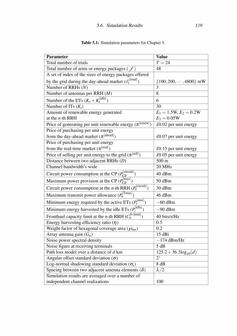
5.6. Simulation Results 119
Table 5.1: Simulation parameters for Chapter 5.
Parameter ValueTotal number of trials T = 24Total number of arms or energy packages (J ) 48A set of index of the sizes of energy packages offeredby the grid during the day-ahead market (E [total]
t ) {100,200, · · · ,4800} mWNumber of RRHs (N) 3Number of antennas per RRH (M) 8Number of the ETs (Ke +K[idle]
e ) 6Number of ITs (Ki) 30Amount of renewable energy generated E1 = 1.5W, E2 = 0.2Wat the n-th RRH E3 = 0.05WPrice of generating per unit renewable energy (π [renew]) £0.02 per unit energyPrice of purchasing per unit energyfrom the day-ahead market (π [ahead]) £0.07 per unit energyPrice of purchasing per unit energyfrom the real-time market (π [real]) £0.15 per unit energyPrice of selling per unit energy to the grid (π [sell]) £0.05 per unit energyDistance between two adjacent RRHs (D) 500 mChannel bandwidth’s wide 20 MHzCircuit power consumption at the CP (P[circuit]
CP ) 40 dBmMaximum power provision at the CP (P[max]
CP ) 50 dBmCircuit power consumption at the n-th RRH (P[circuit]
n ) 30 dBmMaximum transmit power allowance (P[Tmax]
n ) 46 dBmMinimum energy required by the active ETs (P[min]
e ) −60 dBmMinimum energy harvested by the idle ETs (P[idle]
z ) −90 dBmFronthaul capacity limit at the n-th RRH (C[b-limit]
n ) 40 bits/s/HzEnergy harvesting efficiency ratio (η) 0.5Weight factor of hexagonal coverage area (℘nm) 0.2Array antenna gain (Ga) 15 dBiNoise power spectral density −174 dBm/HzNoise figure at receiving terminals 5 dBPath loss model over a distance of d km 125.2+36.3log10(d)Angular offset standard deviation (σ ) 2◦
Log-normal shadowing standard deviation (σs) 8 dBSpacing between two adjacent antenna elements (δ ) λ/2Simulation results are averaged over a number ofindependent channel realizations 100
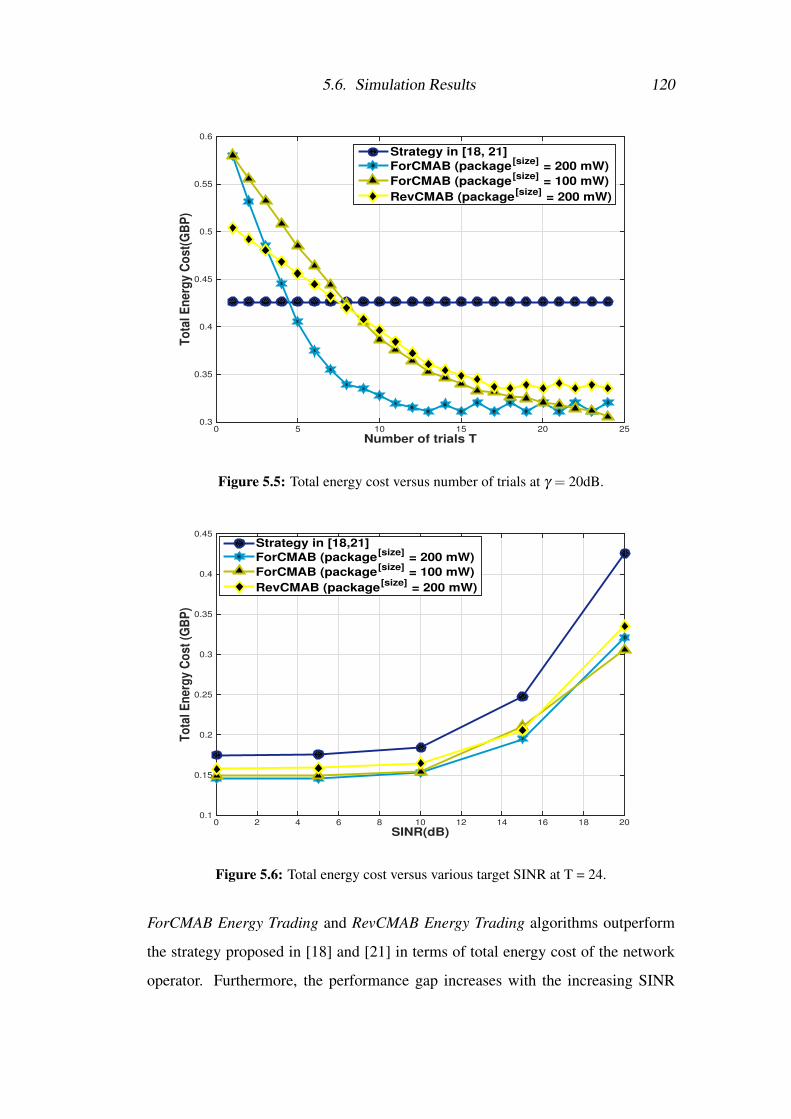
5.6. Simulation Results 120
Number of trials T0 5 10 15 20 25
To
tal E
nerg
y C
ost(
GB
P)
0.3
0.35
0.4
0.45
0.5
0.55
0.6
Strategy in [18, 21]
ForCMAB (package[size]
= 200 mW)
ForCMAB (package[size]
= 100 mW)
RevCMAB (package[size]
= 200 mW)
Figure 5.5: Total energy cost versus number of trials at γ = 20dB.
SINR(dB)0 2 4 6 8 10 12 14 16 18 20
To
tal E
nerg
y C
ost
(GB
P)
0.1
0.15
0.2
0.25
0.3
0.35
0.4
0.45
Strategy in [18,21]
ForCMAB (package[size]
= 200 mW)
ForCMAB (package[size]
= 100 mW)
RevCMAB (package[size]
= 200 mW)
Figure 5.6: Total energy cost versus various target SINR at T = 24.
ForCMAB Energy Trading and RevCMAB Energy Trading algorithms outperform
the strategy proposed in [18] and [21] in terms of total energy cost of the network
operator. Furthermore, the performance gap increases with the increasing SINR
5.7. Concluding Remarks 121
Index of RRH1 2 3
Se
t o
f o
pti
ma
l e
ne
rgy
pa
ck
ag
es
de
cid
ed
b
y C
P d
uri
ng
T t
ria
l (m
W)
0
200
400
600
800
1000
1200
1400
1600
Strategy in [18, 21]
ForCMAB (package[size]
= 200 mW)
ForCMAB (package[size]
= 100 mW)
RevCMAB (package[size]
= 200 mW)
Figure 5.7: Average set of optimal sizes of the energy packages to be purchased from theday-ahead market decided by the CP at T = 24 and γ = 20dB.
requirements.
Figure 5.7 presents in details a set of the optimal energy packages chosen by
the CP to be purchased from the day-ahead market at the 24th trial. It is noticeable
that instead of using a fixed set of energy packages, both of our proposed strategies
purchase a set of optimal energy packages from day-ahead market on the basis of
actual energy generation and the energy requirements at the individual RRHs.
In addition, even though both of the proposed strategies have similar perfor-
mance in terms of total energy cost of the network operator at γ = 20 dB, the pro-
posed RevCMAB Energy Trading algorithm tends to purchase higher amount of
energy packages from the day-ahead market for the individual RRHs.
5.7 Concluding RemarksThis chapter proposes two CMAB algorithms, namely, ForCMAB Energy Trading
and RevCMAB Energy Trading, to observe the instantaneous energy demand and
learn from the behaviour of cooperative energy trading in the green C-RAN with
5.7. Concluding Remarks 122
SWIPT. At each trial, the sparse beamforming technique is employed to find the
optimal trade-off between the cooperative transmission and the total energy cost of
the network operator. Assuming that the RRHs have no initial knowledge of forth-
coming energy consumption and renewable energy production in real-time energy
trading, the CMAB learning process is employed to search for the optimal set of
energy packages to be purchased from the day-ahead market in a limited number
of trials, to further reduce the total energy cost of the network operator. If some
initial knowledge of forthcoming energy consumption or renewable energy produc-
tion are available, then the optimal set of energy packages to be purchased from the
day-ahead market can be searched in a few trials and the accumulated reward can
be maximized. Simulation results confirm that in terms of reducing the total en-
ergy cost of the network operator, both proposed strategies outperform two recently
proposed strategies without CMAB approach in green C-RAN.
Chapter 6
An Online Learning Approach : A
Smart Energy Management
6.1 Introduction
In this chapter, a smart energy management strategy based on the combinato-
rial multi-armed bandit (CMAB) theory for cloud radio access network (C-RAN),
which is powered by a hybrid of grid and renewable energy sources is developed.
A combinatorial upper confidence bound (CUCB) algorithm is introduced to maxi-
mize the overall rewards, earned as a result of minimizing the cost of energy trading
at individual remote radio heads (RRHs) of the C-RAN. Adapting to the dynamic
wireless channel conditions, the proposed CUCB algorithm associates a set of op-
timal energy packages, to be purchased from the day-ahead markets, to a set of
RRHs to minimize the total cost of energy purchase from the main power grid by
dynamically forming super arms. A super arm is formed on the basis of calculat-
ing the instantaneous energy demands at the current time slot, learning from the
cooperative energy trading at the previous time slots and adjusting the mean re-
wards of the individual arms. This chapter further extends the work in chapter 5 as
well as [22] in a more general approach and proposes a CUCB strategy for com-
binatorial generalization of the multi-armed bandit (MAB) problem in the field of
joint management of real-time resource allocation and energy trading. Under the
assumption that prior knowledge of neither the forthcoming power budget nor the
6.2. An Online Learning Approach for A Smart Real-Time Energy Trading 124
amount of energy consumption at individual RRHs are available to the centralized
cloud computing processor (CP), the aim of the proposed strategy in this chapter
is to dynamically determine an optimal set of energy packages for the RRHs to be
purchased from the day-ahead market as per wireless channel conditions at the indi-
vidual time slots, so that the total energy cost of the network operator can be further
reduced. In contrast to the cooperative energy trading designs proposed in the pre-
vious chapter, this chapter proposes a CUCB-CMAB strategy that will estimate the
forthcoming energy demands and select an optimal set of energy packages to be
purchased from the day-ahead market for the next time slot based on the observa-
tion of instantaneous energy demands at the current time slot and learning from the
cooperative energy trading at previous time slots.
6.1.1 Organization
This chapter follows the same system model and problem formulation that have
been proposed for the Dynamic RRH-centric Clustering (DRRHC) with Overall
Energy Purchase Minimization strategy. Please refer to section 5.2, Chapter 5. The
rest of this chapter is organized as follows. In section 6.2, problem formulation
for online learning approach and CUCB-CMAB algorithms, namely CMAB for Su-
per Arm Exploration Algorithm and CUCB-CMAB Main Algorithm are proposed.
Numerical simulation results are analyzed in section 6.3. Finally, section 6.4 sum-
marizes this chapter.
6.2 An Online Learning Approach for A Smart Real-
Time Energy Trading
6.2.1 Problem Formulation for Online Learning Approach
The CP applies CMAB to adapt its energy trading strategies to the intermittent
environment in C-RAN by dynamically forming super arms to maximize the accu-
mulated rewards, which is equivalent to minimizing the total cost of the network
operator. A super arm is composed of a set of arms and each arm corresponds to the
size of an energy package to be purchased for an RRH from the day-ahead market
6.2. An Online Learning Approach for A Smart Real-Time Energy Trading 125
prior to the actual time of energy demand.
Let J = {1, · · · ,J} indicate a set of indexes for possible energy packages of-
fered in the day-ahead market by the grid. At each trial, the CP allocates a super arm
composed of N arms, i.e., N sizes of energies out of J possible energy packages, to
N RRHs. Since, this is equivalent to choosing simultaneously a set of N arms from
J possible arms, the involved MAB problem is categorized as the CMAB prob-
lem [16]. Let E [total] = {E 1, · · · ,E J} represent the set of sizes of energy packages
offered by the grid in the day-ahead market, where E 1 < E 2 < · · ·< E J is an arith-
metic progression with a common difference of ∆E , i.e., E p = E p−1+∆E , p ∈J .
Furthermore, let A[set]
k = {B[ahead]1 (k), · · · ,B[ahead]
N (k)} denote a set of N energy
sizes, i.e., a super arm, to be purchased for N RRHs by the network operator from
the day-ahead market at the k-th trial. Then, the total energy cost of the network
operator incurred by the n-th RRH at the k-th trial, i.e., B[total]n (k), can be calculated
as
B[total]n (k) = π
[ahead]B[ahead]n (k)+π
[real]B[real]n (k) (6.1)
+π[renew]En(k)−π
[sell]Sn(k), ∀n ∈Lb.
Let further define the individual reward for the n-th RRH and the overall reward
for the super arm at the k-th trial as R(B[ahead]n (k)) and R(A
[set]k ), respectively, as
follows
R(B[ahead]n (k)) = B[total]
n (1)−B[total]n (k),∀n ∈Lb, (6.2)
R(A[set]
k ) = ∑n∈Lb
R(B[ahead]n (k)), (6.3)
where B[total]n (1) and B[total]
n (k) in (6.2) are the total energy cost of the network oper-
ator incurred by the n-th RRH, respectively, at the initial trial and the k-th trial of a
frame. Let K = {1, · · · ,K}, F = {1, · · · ,F} and T = {1, · · · ,T} be respectively
associated to the set of indexes of the trials within a frame, the set of indexes of the
frames within a time slot and the set of indexes of the time slots.
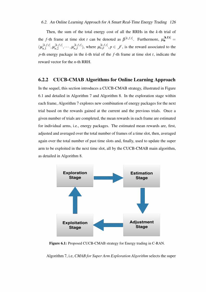
6.2. An Online Learning Approach for A Smart Real-Time Energy Trading 126
Then, the sum of the total energy cost of all the RRHs in the k-th trial of
the f -th frame at time slot t can be denoted as β [k, f ,t]. Furthermore, µ[k,f,t]n =
(µ[k, f ,t]n,1 ,µ
[k, f ,t]n,2 , · · · ,µ [k, f ,t]
n,J ), where µ[k, f ,t]n,p , p ∈J , is the reward associated to the
p-th energy package in the k-th trial of the f -th frame at time slot t, indicate the
reward vector for the n-th RRH.
6.2.2 CUCB-CMAB Algorithms for Online Learning Approach
In the sequel, this section introduces a CUCB-CMAB strategy, illustrated in Figure
6.1 and detailed in Algorithm 7 and Algorithm 8. In the exploration stage within
each frame, Algorithm 7 explores new combination of energy packages for the next
trial based on the rewards gained at the current and the previous trials. Once a
given number of trials are completed, the mean rewards in each frame are estimated
for individual arms, i.e., energy packages. The estimated mean rewards are, first,
adjusted and averaged over the total number of frames of a time slot, then, averaged
again over the total number of past time slots and, finally, used to update the super
arm to be exploited in the next time slot, all by the CUCB-CMAB main algorithm,
as detailed in Algorithm 8.
!
Exploration !Stage!
!
!!
Exploitation !Stage!
!
!
Estimation !Stage!
!
!
Adjustment!Stage!
!
Figure 6.1: Proposed CUCB-CMAB strategy for Energy trading in C-RAN.
Algorithm 7, i.e, CMAB for Super Arm Exploration Algorithm selects the super
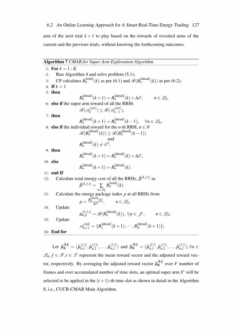
6.2. An Online Learning Approach for A Smart Real-Time Energy Trading 127
arm of the next trial k + 1 to play based on the rewards of revealed arms of the
current and the previous trials, without knowing the forthcoming outcomes.
Algorithm 7 CMAB for Super Arm Exploration Algorithm.1: For k = 1 : K2: Run Algorithm 4 and solve problem (5.1);3: CP calculates B[total]
n (k) as per (6.1) and R(B[ahead]n (k)) as per (6.2);
4: If k = 15: then
B[ahead]n (k+1) = B[ahead]
n (k)+∆E , n ∈Lb.6: else if the super arm reward of all the RRHs
R(A[set]
k )≤R(A[set]
k−1 ),7: then
B[ahead]n (k+1) = B[ahead]
n (k−1), ∀n ∈Lb,8: else if the individual reward for the n-th RRH, n ∈ N
R(B[ahead]n (k))≥R(B[ahead]
n (k−1))and
B[ahead]n (k) 6= E J ,
9: thenB[ahead]
n (k+1) = B[ahead]n (k)+∆E ,
10: elseB[ahead]
n (k+1) = B[ahead]n (k).
11: end If12: Calculate total energy cost of all the RRHs, β [k, f ,t] as
β [k, f ,t] = ∑n∈Lb
B[total]n (k).
13: Calculate the energy package index p at all RRHs from
p = B[ahead]n (k)
∆E , n ∈Lb.14: Update
µ[k, f ,t]n,p = R(B[ahead]
n (k)), ∀p ∈J , n ∈Lb;15: Update
A[set]
k+1 = {B[ahead]1 (k+1), · · · ,B[ahead]
N (k+1)};16: End for
Let µ[f,t]n = (µ
[ f ,t]n,1 , µ
[ f ,t]n,2 , . . . , µ
[ f ,t]n,J ) and µ
[f,t]n = (µ
[ f ,t]n,1 , µ
[ f ,t]n,2 , . . . , µ
[ f ,t]n,J ),∀n ∈
Lb, f ∈F , t ∈ T represent the mean reward vector and the adjusted reward vec-
tor, respectively. By averaging the adjusted reward vector µ[f,t]n over F number of
frames and over accumulated number of time slots, an optimal super arm S∗ will be
selected to be applied in the (t +1)-th time slot as shown in detail in the Algorithm
8, i.e., CUCB-CMAB Main Algorithm.
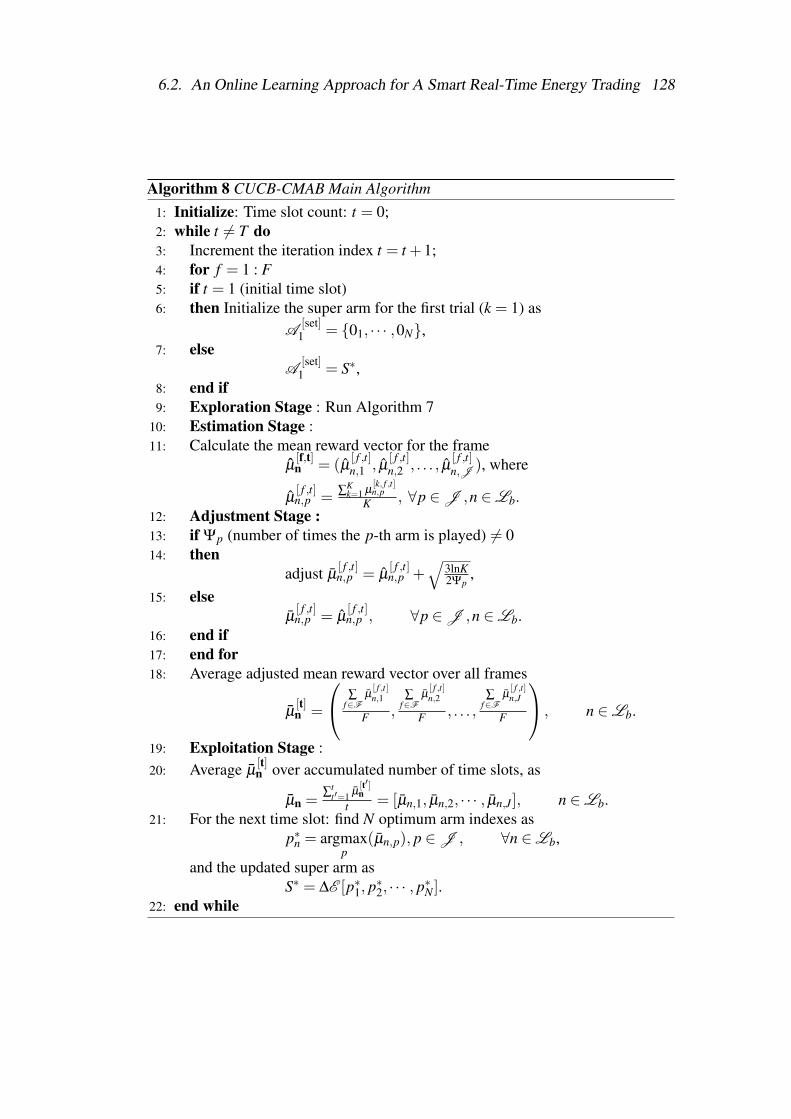
6.2. An Online Learning Approach for A Smart Real-Time Energy Trading 128
Algorithm 8 CUCB-CMAB Main Algorithm1: Initialize: Time slot count: t = 0;2: while t 6= T do3: Increment the iteration index t = t +1;4: for f = 1 : F5: if t = 1 (initial time slot)6: then Initialize the super arm for the first trial (k = 1) as
A[set]
1 = {01, · · · ,0N},7: else
A[set]
1 = S∗,8: end if9: Exploration Stage : Run Algorithm 7
10: Estimation Stage :11: Calculate the mean reward vector for the frame
µ[f,t]n = (µ
[ f ,t]n,1 , µ
[ f ,t]n,2 , . . . , µ
[ f ,t]n,J ), where
µ[ f ,t]n,p = ∑
Kk=1 µ
[k, f ,t]n,p
K , ∀p ∈J ,n ∈Lb.12: Adjustment Stage :13: if Ψp (number of times the p-th arm is played) 6= 014: then
adjust µ[ f ,t]n,p = µ
[ f ,t]n,p +
√3lnK2Ψp
,15: else
µ[ f ,t]n,p = µ
[ f ,t]n,p , ∀p ∈J ,n ∈Lb.
16: end if17: end for18: Average adjusted mean reward vector over all frames
µ[t]n =
∑f∈F
µ[ f ,t]n,1
F ,∑
f∈Fµ[ f ,t]n,2
F , . . . ,∑
f∈Fµ[ f ,t]n,J
F
, n ∈Lb.
19: Exploitation Stage :20: Average µ
[t]n over accumulated number of time slots, as
µn =∑
tt′=1 µ
[t′]n
t = [µn,1, µn,2, · · · , µn,J], n ∈Lb.21: For the next time slot: find N optimum arm indexes as
p∗n = argmaxp
(µn,p), p ∈J , ∀n ∈Lb,
and the updated super arm asS∗ = ∆E [p∗1, p∗2, · · · , p∗N ].
22: end while
6.3. Simulation Results 129
6.3 Simulation Results
The simulation considers a downlink C-RAN consists of 3 adjacent RRHs towards
6 single-antenna information receiving terminals (ITs) and 6 single-antenna energy
receiving terminals (ETs). Each RRH is equipped with 8 antennas and located 500m
away from each other. The performance of the proposed approach is evaluated with
K = 10 trials per frame, F = 10 frames per time slot, T = 60 time slots, J = 20
energy packages and ∆E = 100 mW, i.e., E[total]k = {100,200, · · · ,2000} mW. The
renewable energy generation at each RRH is assumed to be E1 = 1.5 W, E2 = 0.2
W and E3 = 0.05 W, respectively, at price of π [renew] = £0.02/W. The network op-
erator purchases a set of energy packages from the day-ahead market at a price of
π [ahead] = £0.07/W and from the real-time market at a price of π [real] = £0.15/W
and sell excessive energy back to the grid at a price of π [sell] = £0.05/W. A corre-
lated channel model hni = R1/2hw is adopted, where hw ∈ CM×1 are zero mean
circularly symmetric complex Gaussian (ZMCSCG) random variables with unit
variance, R ∈ CM×M is the spatial covariance matrix and its (m,n)-th element is
given by GaLpσ2Fe−0.5 (σs ln10)2
100 e j 2πδ
λ[(n−m)sinθ ]e−2[ πδσ
λ(n−m)cosθ ]
2
, where Ga = 15 dBi
is antenna gain, Lp(dB) = 125.2+ 36.3log10(d) is the path loss model over a dis-
tance of d km, σ2F is the variance of the complex Gaussian fading coefficient, σs = 8
dB is the log-normal shadowing standard deviation, δ = λ/2 is the antenna spac-
ing, σ = 2◦ is the angular offset standard deviation and θ is the estimated angle
of departure. The channel bandwidth, noise figure at receiving terminals and noise
power spectral density are set to be 20 MHz, 5 dB and −174 dBm/Hz, respectively.
Besides, the parameters for optimization constraints are assumed, unless otherwise
stated, to be P[circuit]CP = 40 dBm, P[max]
CP = 50 dBm, P[circuit]n = 30 dBm, P[Tmax]
n = 46
dBm, C[b-limit]n = 30 bits/s/Hz, γi = 20dB, P[min]
e = −60 dBm, P[idle]z = −90 dBm
and η = 0.5. The simulation results are efficiently obtained and averaged over 100
independent channel realizations via CVX [108]. The list of parameters used in this
simulation are summarized in Table 6.1.
The proposed learning-based approach is compared against the baseline strat-
egy, which does not consider purchasing energy packages from the day-ahead mar-
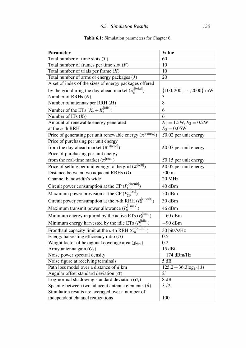
6.3. Simulation Results 130
Table 6.1: Simulation parameters for Chapter 6.
Parameter ValueTotal number of time slots (T ) 60Total number of frames per time slot (F) 10Total number of trials per frame (K) 10Total number of arms or energy packages (J) 20A set of index of the sizes of energy packages offeredby the grid during the day-ahead market (E [total]
k ) {100,200, · · · ,2000} mWNumber of RRHs (N) 3Number of antennas per RRH (M) 8Number of the ETs (Ke +K[idle]
e ) 6Number of ITs (Ki) 6Amount of renewable energy generated E1 = 1.5W, E2 = 0.2Wat the n-th RRH E3 = 0.05WPrice of generating per unit renewable energy (π [renew]) £0.02 per unit energyPrice of purchasing per unit energyfrom the day-ahead market (π [ahead]) £0.07 per unit energyPrice of purchasing per unit energyfrom the real-time market (π [real]) £0.15 per unit energyPrice of selling per unit energy to the grid (π [sell]) £0.05 per unit energyDistance between two adjacent RRHs (D) 500 mChannel bandwidth’s wide 20 MHzCircuit power consumption at the CP (P[circuit]
CP ) 40 dBmMaximum power provision at the CP (P[max]
CP ) 50 dBmCircuit power consumption at the n-th RRH (P[circuit]
n ) 30 dBmMaximum transmit power allowance (P[Tmax]
n ) 46 dBmMinimum energy required by the active ETs (P[min]
e ) −60 dBmMinimum energy harvested by the idle ETs (P[idle]
z ) −90 dBmFronthaul capacity limit at the n-th RRH (C[b-limit]
n ) 30 bits/s/HzEnergy harvesting efficiency ratio (η) 0.5Weight factor of hexagonal coverage area (℘nm) 0.2Array antenna gain (Ga) 15 dBiNoise power spectral density −174 dBm/HzNoise figure at receiving terminals 5 dBPath loss model over a distance of d km 125.2+36.3log10(d)Angular offset standard deviation (σ ) 2◦
Log-normal shadowing standard deviation (σs) 8 dBSpacing between two adjacent antenna elements (δ ) λ/2Simulation results are averaged over a number ofindependent channel realizations 100
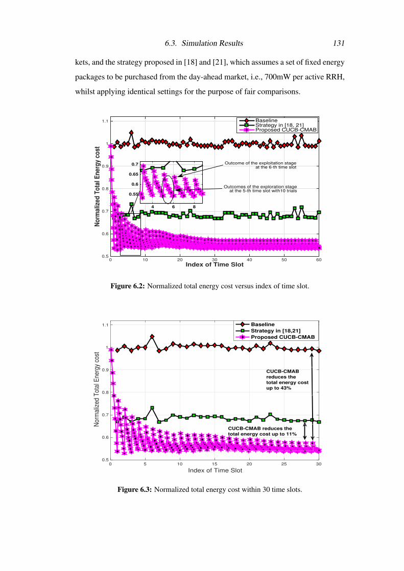
6.3. Simulation Results 131
kets, and the strategy proposed in [18] and [21], which assumes a set of fixed energy
packages to be purchased from the day-ahead market, i.e., 700mW per active RRH,
whilst applying identical settings for the purpose of fair comparisons.
Index of Time Slot0 10 20 30 40 50 60
No
rmal
ized
To
tal E
ner
gy
cost
0.5
0.6
0.7
0.8
0.9
1
1.1 BaselineStrategy in [18, 21]Proposed CUCB-CMAB
4 6 8
0.55
0.6
0.65
0.7 Outcome of the exploitation stageat the 6-th time slot
Outcomes of the exploration stageat the 5-th time slot with10 trials
Figure 6.2: Normalized total energy cost versus index of time slot.
0 5 10 15 20 25 30
Index of Time Slot
0.5
0.6
0.7
0.8
0.9
1
1.1
Nor
mal
ized
Tot
al E
nerg
y co
st
Baseline
Strategy in [18,21]
Proposed CUCB-CMAB
CUCB-CMAB
reduces the
total energy cost
up to 43%
CUCB-CMAB reduces the
total energy cost up to 11%
Figure 6.3: Normalized total energy cost within 30 time slots.
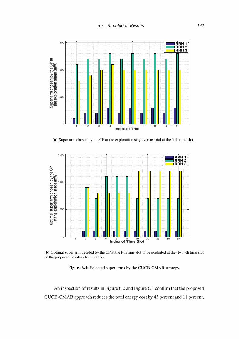
6.3. Simulation Results 132
Index of Trial1 2 3 4 5 6 7 8 9 10
Su
per
arm
ch
ose
n b
y th
e C
P a
t th
e ex
plo
rati
on
sta
ge
(mW
)
0
500
1000
1500 RRH 1RRH 2RRH 3
(a) Super arm chosen by the CP at the exploration stage versus trial at the 5-th time slot.
Index of Time Slot1 2 3 4 5 10 15 20 25 30 60
Op
tim
al s
up
er a
rm c
ho
sen
by
the
CP
at
th
e ex
plo
itat
ion
sta
ge
(mW
)
0
500
1000
1500
RRH 1RRH 2RRH 3
(b) Optimal super arm decided by the CP at the t-th time slot to be exploited at the (t+1)-th time slotof the proposed problem formulation.
Figure 6.4: Selected super arms by the CUCB-CMAB strategy.
An inspection of results in Figure 6.2 and Figure 6.3 confirm that the proposed
CUCB-CMAB approach reduces the total energy cost by 43 percent and 11 percent,
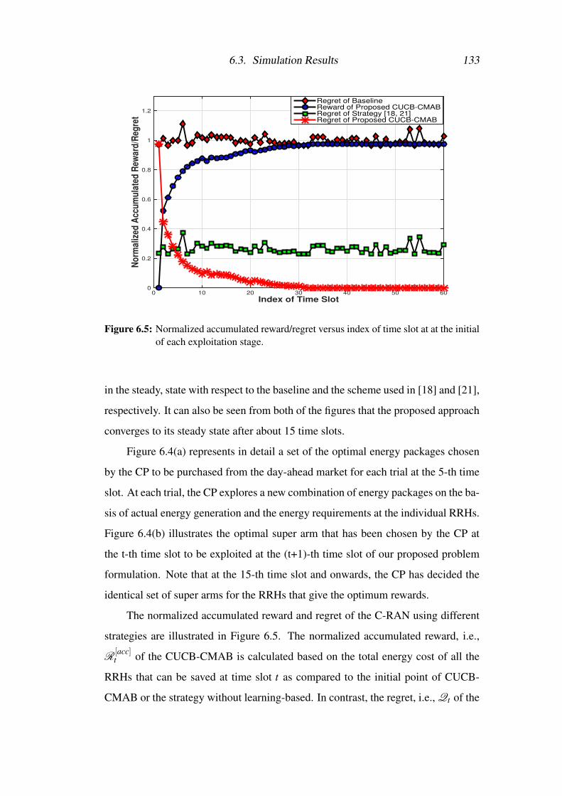
6.3. Simulation Results 133
Index of Time Slot0 10 20 30 40 50 60
No
rmal
ized
Acc
um
ula
ted
Rew
ard
/Reg
ret
0
0.2
0.4
0.6
0.8
1
1.2
Regret of BaselineReward of Proposed CUCB-CMABRegret of Strategy [18, 21]Regret of Proposed CUCB-CMAB
Figure 6.5: Normalized accumulated reward/regret versus index of time slot at at the initialof each exploitation stage.
in the steady, state with respect to the baseline and the scheme used in [18] and [21],
respectively. It can also be seen from both of the figures that the proposed approach
converges to its steady state after about 15 time slots.
Figure 6.4(a) represents in detail a set of the optimal energy packages chosen
by the CP to be purchased from the day-ahead market for each trial at the 5-th time
slot. At each trial, the CP explores a new combination of energy packages on the ba-
sis of actual energy generation and the energy requirements at the individual RRHs.
Figure 6.4(b) illustrates the optimal super arm that has been chosen by the CP at
the t-th time slot to be exploited at the (t+1)-th time slot of our proposed problem
formulation. Note that at the 15-th time slot and onwards, the CP has decided the
identical set of super arms for the RRHs that give the optimum rewards.
The normalized accumulated reward and regret of the C-RAN using different
strategies are illustrated in Figure 6.5. The normalized accumulated reward, i.e.,
R[acc]t of the CUCB-CMAB is calculated based on the total energy cost of all the
RRHs that can be saved at time slot t as compared to the initial point of CUCB-
CMAB or the strategy without learning-based. In contrast, the regret, i.e., Qt of the
6.4. Concluding Remarks 134
models can be defined as Qt = R[acc]opt −R
[acc]t , where R
[acc]opt is the optimum reward
that can be obtained using our learning based strategy. It can be observed from
Figure 6.5 that a significant performance gap exists between the proposed CUCB-
CMAB and the baseline scheme as well as the strategy in [18] and [21]. Even
though the regret of the CUCB-CMAB strategy is worst at the beginning of the
learning process, the regrets start to drop at a great rate with the increasing number
of time slots.
6.4 Concluding RemarksThis chapter proposes an online learning approach for a smart energy management
strategy based on the CMAB approach for green C-RAN with SWIPT. The CUCB-
CMAB algorithms are introduced to adapt to the dynamic wireless channel con-
ditions to further minimize the total energy cost of the network operator by maxi-
mizing the accumulated rewards obtained at each iteration. The CP calculates and
learns the instantaneous energy demand at the current and previous time slots and
decides the optimal set of energy packages to be purchased from the day-ahead mar-
ket for the forthcoming cooperative energy trading. Our simulation results confirm
that the total energy cost can be saved up to 43 percent as compared to the baseline
strategy and up to 11 percent as compared to the latest scheme in energy trading
without any learning-based approach.
Chapter 7
Conclusions and Future Research
7.1 Thesis Summary
Denser site deployment has been regarded as a key enabling technology to sup-
port gigantic increasing mobile data traffic and high data rate communications with
ubiquitously guaranteed quality of service (QoS) for next generation wireless com-
munication networks [1]. However, the significant inter-cell interference (ICI) may
limit the performance of the system. Cloud radio access network (C-RAN) has illus-
trated its considerable advantages in ICI mitigation as well as reducing both of the
capital expenditure (CAPEX) and the operating expense (OPEX) of the network op-
erator. In a C-RAN architecture, the conventional base stations (BSs) are physically
detached into two parts: baseband processing units (BBUs) that are grouped into a
BBU pool, i.e., a centralized cloud computing processor (CP), which is responsible
for all the coordination and energy trading strategies, and the remaining remote ra-
dio heads (RRHs), that are in charge of all radio frequency operations. The data of
information receiving terminals (ITs) is available at the CP and will be delivered to
the multiple collaborative RRHs via high-capacity low-latency fronthaul links, e.g.,
optical fibre links. On the other hand, the ever-increasing energy cost has become
a major OPEX as a result of striking rise of energy consumption induced by the
ultra-dense RRHs deployment, which may result in a revenue threshold of the net-
work operator. Consequently, equipping the RRHs with green energy technology
that can harvest energy from environmental sources at a lower price for powering

7.1. Thesis Summary 136
next generation mobile communication networks, has become the potential solu-
tion. The local renewable energy generation in practice is, nevertheless, unequal
since it highly depends on the efficiency of renewable energy harvesting devices
and the location of installation sites. With the advanced smart grid technology, the
implementation of two-way energy trading with the grid allows the RRHs to main-
tain their reliable operation in the case of insufficient local renewable energy via
purchasing the inadequate amount of energy from the grid. Therefore, the network
operator can maximally benefit from utilizing the local renewable energy and by
selling the excessive energy back to the grid on an agreed price. Nevertheless, the
aggregated power requirements by both receiving terminals may exceed the amount
of power budget at the RRHs. Hence, the network operator has to purchase addi-
tional energy from the real-time market from the smart grid with a higher price, and
may take a risk of losing the profit.
The introductory chapter consists of an outlined of the thesis statement that
defines the open issues regarding interference and operational costs managements
for next generation networks. Furthermore, the contributions of this thesis which
are organized based on each subsequent chapters and a list of publications that are
related to this thesis also have been highlighted.
Fundamental concepts of related topics were briefly reviewed in Chapter 2. A
common class of optimal transmit downlink beamforming for multiple receiving
terminals in a C-RAN powered by renewable energy technologies also has been
provided in order to calculate the total transmit power with the given constraints.
This non-convex optimization problem was transformed into a convex optimization
form and the rank1 constraint has been relaxed by using semidefinite programming
(SDP) and semidefinite relaxation (SDR) approaches, respectively. Furthermore,
a resource management and energy trading approach for energy cost saving in C-
RAN powered by two-way energy cooperation between the smart grid and the re-
newable energy technologies has been introduced to adjust the non-uniform energy
supplies and energy demands over the C-RAN. Related works comparable to the
raised issues in the thesis are also discussed in this chapter.
7.1. Thesis Summary 137
Three different cooperative real-time energy trading strategies for downlink
green C-RAN have been proposed in the first major contribution chapter, Chapter
3. The main objective was to jointly minimize the energy consumption and the real-
time energy trading under the constraints of demand and supply power balancing at
RRHs and QoS required by the information receiving terminals. For strategy 1, a
sparse beamforming problem was formulated as an `0-norm optimization problem
and solve it using SDR and iterative reweighted `1-norm approximation of `0-norm.
The strategies 2 and 3 were formulated as numerically tractable optimization prob-
lem and solved using the SDR approach. It has been proved that in terms of reduc-
ing total energy cost of the network operator, significant performance gain can be
achieved by all the three proposed joint cooperative transmission and energy trading
strategies, as compared to a baseline scheme that separately optimize the coopera-
tive transmission and energy trading in a C-RAN scenario with realistic parameter
settings.
A real-time energy trading strategy with simultaneous wireless information
and power transfer (SWIPT) concept has been integrated in Chapter 4. Instead of
designing the energy management for individual RRHs with a shortage of power
as proposed in the previous chapter, the design strategies in Chapter 4 account for
all RRHs with or without a shortage of power. The proposed strategies strike an
optimum balance between the total power consumption in the fronthaul through ad-
justing the degree of partial cooperation among RRHs, RRHs’ total transmit power
and their maximum or total energy-purchase from the real-time market. Two strate-
gies for optimizing the RRHs’ real-time energy trading with the smart grid have
been presented. The first strategy was for minimizing the RRHs’ maximum real-
time energy-purchase requests and the second strategy for minimizing the RRHs’
overall energy-purchase requests from the real-time market. Unlike Chapter 3 that
take no consideration of realistic constraints on fronthaul capacity restrictions, this
chapter was formulated with more realistic scenarios where RRHs was constrained
with limited fronthaul capacities. An iterative energy receiving terminal (ET) autho-
rization algorithm that allows only those ETs situated close enough to the RRHs to

7.1. Thesis Summary 138
receive wireless energy was introduced in order to maintain the efficiency of SWIPT
technology. By employing the reweighted `1-norm approximation for `0-norm and
SDR, the solution sparsity to the original non-convex optimization problems in (4.7)
and (4.11) can be obtained. Simulation results confirmed that both of the proposed
strategies outperform two other recently proposed schemes in terms of improving
the energy efficiency and reducing total energy cost of the RRH in a realistic C-RAN
scenario.
The works in previous chapters have been extended to a learning-based prac-
tical approach in Chapter 5. With various sizes of energy packages which were
offered in the day-ahead market, the new responsibility of the CP is to determine
the set of optimal sizes of the energy packages to be purchased for the RRHs on
the basis of actual energy supply and demand, to further minimize the total en-
ergy cost of the network operator. Assuming that the RRHs have no initial knowl-
edge of forthcoming energy consumption and renewable energy production in real-
time energy trading, two combinatorial multi-armed bandit (CMAB) learning algo-
rithms, namely, Forward CMAB (ForCMAB) Energy Trading and Reverse CMAB
(RevCMAB) Energy Trading, have been proposed to observe the instantaneous en-
ergy demand and learn from the behaviour of cooperative energy trading in the
green C-RAN with SWIPT. Simulation results confirmed that the two CMAB learn-
ing strategies outperform the strategies without learning approach, in terms of fur-
ther reducing the total energy cost of the network operator.
A smart energy management strategy based on the CMAB approach for green
C-RAN with SWIPT has been proposed in the last contribution chapter, Chapter 6.
The combinatorial upper confidence bound (CUCB)-CMAB algorithms were intro-
duced to adapt to the dynamic wireless channel conditions to further minimize the
total energy cost of the network operator by maximizing the accumulated rewards
obtained at each iteration. In contrast to the cooperative energy trading designs
proposed in chapter 5, the CUCB-CMAB strategy will estimate the forthcoming
energy demands and select an optimal set of energy packages to be purchased from
the day-ahead market for the next time slot based on the observation of instanta-
7.2. Avenues of Future Research 139
neous energy demands at the current time slot and learning from the cooperative
energy trading at previous time slots. Even though the regret of the CUCB-CMAB
strategy is worst at the beginning of the learning process, the regrets start to drop
at a great rate with the increasing number of time slots. It has been illustrated from
the simulation results that the total energy cost can be saved up to 43 percent as
compared to the baseline strategy and up to 11 percent as compared to the strategy
without any learning-based approach.
7.2 Avenues of Future ResearchContinuing from the aforementioned studies on energy and communication cooper-
ation presented in this thesis, the current section suggests interesting directions for
future research.
7.2.1 Self Energy Storage
In this thesis, no RRH in the green C-RAN is equipped with frequently rechargeable
storage devices due to the cost consideration. However, in future, it is not impos-
sible to install an energy storage at the master base station (MBS) in the C-RAN
or can be employed at the RRHs with the advancement of battery technologies.
The self energy storage management is expected to control unequal local renewable
energy generation to match the energy request by receiving terminals that always
change over time.
7.2.2 Neighbourhood Energy Sharing and Trading
Interestingly, self energy storages at the RRHs promote the neighbourhood energy
sharing and cooperation in the C-RAN. Yet, how to enable energy sharing and co-
operation between the RRHs requires communication compatibility and more co-
ordination at the CP. Moreover, this collaboration can be expanded to the multiple
self-interest systems that has been owned by different network operators. In this
configuration, the CP at each C-RAN needs to establish a genuine joint energy and
communication cooperation, since any present decisions made by the CPs would
affect their total energy request to be served in the future. Presume in the energy
sharing management, one selfish CP may request extra energy from the CP of the
7.2. Avenues of Future Research 140
other C-RAN and sell the energy to the grid to make a profit. Therefore, energy
trading inter-system also need to be considered.
7.2.3 Game Theoretical Approach
To further motivate the potential RRHs with extra energy to assist in neighbour-
hood energy sharing and trading, practical energy and communications cooperation
mechanisms need to be designed for RRHs by the game theoretical approach. For
example, the RRHs could be selfish and prefer to store the harvested energy rather
than to cooperate with the other RRHs. In this situation, that particular RRHs need
to be offered some extra incentive to encourage them to be good players in a game.
A good cooperation mechanism design is required to motivate all the players in a
huge network cooperation to support the inter-system joint cooperation to a win-win
situation for all systems involved.
7.2.4 Robust Sparse Beamforming
The sparse beamforming strategy used in this thesis works on the assumption that
the cooperative transmitters have very accurate channel state information (CSI)
about each others channel towards the receiver. In reality, however, the obtained
CSI is not always accurate, e.g., due to location estimation errors. In such a case,
sparse beamforming fails since the signals that arrive at the receiver are not syn-
chronized or because the beamforming weights are not properly distributed among
the cooperating nodes. Therefore, sparse beamforming should be made robust to
such errors.
7.2.5 Multiple Input Multiple Output (MIMO)
In addition, both type of receiving terminals, i.e., ITs and ETs, and RRHs in C-RAN
can be equipped with multiple antennas, i.e, multiple input multiple output (MIMO)
configuration. With MIMO configuration, there will be more degree of freedom to
effectively control interference. On the other hand, transmit and receive beamform-
ing should be jointly designed. A question arising here is whether global optimality
can be achieved by iteratively optimising transmit and receive beamforming. Com-
plexity and signaling overhead are expected to significantly increase. Therefore,

7.2. Avenues of Future Research 141
practical solutions to the optimal beamforming and tradeoff between optimality and
complexity are open problems for research.
Appendix A
Proof of Lemma 1
This section provides a proof for lemma 1 in the context of optimization problem
in (4.10), which can be similarly extended to the context of the optimization prob-
lem in (4.12). Since the optimization problem in (4.10) is convex and satisfies the
Slater’s condition, strong duality holds [68] and its Lagrangian is
L (Wi,Ve,χ,Yi,Ze,νi,ρe,πz,ϕn,φn,τn,ψ,εn,ρn,ςn)
= ∑i∈Li
tr(QiWi)− ∑i∈Li
tr(Wi(Yi +νiHi
γi))
+ ∑e∈Le
tr(QeVe)− ∑e∈Le
tr(Ve(Ze +ρeGe
P[min]e
))+Ξ, (A.1)
where
Qi = α ∑n∈Lb
ξniDn +β I+ ∑i∈Li, j 6=i
ν jH j− ∑e∈Le
ρeGe
P[min]e
− ∑z∈L [idle]
e
Fzπz + ∑n∈Lb
(ϕn +φn + τnξniRi)Dn, (A.2)
Qe = α ∑n∈Lb
κneDn +β I+ ∑i∈Li
νiHi− ∑e∈Le, j 6=e
ρeG j
P[min]e
− ∑z∈L [idle]
e
Fzπz + ∑n∈Lb
(ϕn +φn)Dn, (A.3)
143
Ξ = ∑n∈Lb
(ψ−ϕn)B[ahead]n + ∑
n∈Lb
(ψ−ϕn− εn)B[real]n
+ ∑i∈Li
νiσ2i + ∑
e∈Le
ρeη−1 + ∑
z∈L [idle]e
πzP[idle]z η
−1−ψP[max]CP
− ∑n∈Lb
[ϕn(En−Sn−P[circuit]n )+φnP[Tmax]
n ]+ψP[circuit]CP
− ∑n∈Lb
(τnC[b-limit]n +ρnSn− ςnχ− ςnζ B[real]
n )+χ. (A.4)
Ξ is the summation of the terms that does not involve any Wi and Ve. The matrices
Yi and Ze as well as the set Θ = {νi,ρe,πz,ϕn,φn,τn,ψ,εn,ρn,ςn} denote, respec-
tively, the matrix dual variable of C11 and C12 as well as the set of scalar Lagrange
multipliers of the primal constraints C1-C10. Then, the dual problem can be written
as
maxΘ≥0,Yi,Ze�0
minWi,Ve,χ
L (Wi,Ve,χ,Yi,Ze,Θ), (A.5)
where Θ ≥ 0 implies that all of the scalar dual variables within the set Θ are non-
negative, for the sake of notational simplicity. Let {W∗i ,V∗e ,χ∗} and {Y∗i ,Z∗e ,Θ∗}
be defined as the set of optimal primal and dual variables of (4.10), respectively.
The dual problem in (A.5) can be expressed as
minWi
L (Wi,V∗e ,χ∗,Y∗i ,Z
∗e ,Θ
∗), (A.6)
minVe
L (Ve,W∗i ,χ∗,Y∗i ,Z
∗e ,Θ
∗), (A.7)
and the Karush-Kuhn-Tucker (KKT) conditions are given by
Θ∗ ≥ 0, Y∗i � 0, Y∗i W∗i = 0, ∀i ∈Li, (A.8)
Z∗e � 0, Z∗eV∗e = 0, ∀e ∈Le, (A.9)
Q∗i − (Y∗i +ν∗i Hi
γi) = 0, ∀i ∈Li, (A.10)
Q∗e− (Z∗e +ρ∗e Ge
P[min]e
)) = 0, ∀e ∈Le, (A.11)
144
where Q∗i and Q∗e are obtained by substituting the optimal dual variables into the ex-
pressions in (A.2) and (A.3), respectively. In the sequel, it is shown by contradiction
that rank(V∗e)≤ 1 holds with probability one. It is first proved by contradiction that
Q∗e is a positive definite matrix with probability one. Assuming Q∗e is a non-positive
definite matrix, one of the optimal solutions of (A.7) can be chosen as Ve = hvevHe ,
where h > 0 is a scaling factor and ve is the eigenvector corresponding to one of the
non-positive eigenvalues of Q∗e . Substituting Ve = hvevHe into (A.7) gives
minVe
L (Ve,W∗i ,χ∗,Y∗i ,Z
∗e ,Θ
∗) (A.12)
= ∑e∈Le
tr(hQ∗evevHe )− h ∑
e∈Le
tr(vHe (Z
∗e +
ρ∗e Ge
P[min]e
)ve)
+
(∑
i∈Li
tr(Q∗i W∗i )− ∑i∈Li
tr(W∗i (Y
∗i +
ν∗i Hi
γi))+Θ
∗),
where ∑e∈Le
tr(hQ∗evevHe ) is non-positive and as h→∞,−h ∑
e∈Le
tr(vHe (Z∗e +
ρ∗e Ge
P[min]e
)ve)
may go to negative infinity, which results in an unbounded dual optimal value. How-
ever, the optimal value of the primal problem is non-negative, thus strong duality
does not hold which induces a contradiction. Therefore, Q∗e is a positive definite
matrix with probability one and rank(Q∗e) = MN, provided that channel vectors hi,
ge and fz are independently distributed. Then the following inequality holds as per
(A.11) and properties of rank of matrix:
rank(Q∗e) = MN = rank(Z∗e +ρ∗e Ge
P[min]e
)
≤ rank(Z∗e)+ rank(ρ∗e Ge
P[min]e
)
⇒ rank(Z∗e)≥MN−1. (A.13)
Furthermore, the KKT condition in (A.9), i.e., Z∗eV∗e = 0, implies
rank(Z∗e)≤MN− rank(V∗e). (A.14)
145
If the desired P[min]e is larger than the power that can be transferred to the ET by the
ambient interference, then V∗e 6= 0, otherwise V∗e = 0. On the other hand, an inspec-
tion of the results in (A.13) and (A.14) implies that for V∗e 6= 0, rank(Z∗e) = MN−1
must hold. Note also that according to the KKT condition in (A.9), the columns of
V∗e are in the null space of Z∗e . Therefore, when Ve 6= 0, rank(V∗e) = 1 holds with
probability one, whereas V∗e = 0 implies rank(V∗e) = 0. Hence, rank(V∗e)≤ 1 holds
with probability one.
By following the similar steps, it can be easily shown that in order to satisfy
the minimum SINR requirements in the constraint C1 of (4.12), rank(W∗i ) = 1 must
hold with probability one. This thus completes the proof of Lemma1 for problem
(4.10). Furthermore, Lemma1 also holds for the optimization problem in (4.12)
and can be proven straightforwardly by following the similar steps as stated for the
optimization problem in (4.10).
Bibliography
[1] M. Peng et al., Fronthaul-Constrained Cloud Radio Access Networks: In-
sights and Challenges, In IEEE Wireless Commun., vol. 22, no. 2, pp. 152 -
160, April 2015.
[2] M. Peng et al., Heterogeneous Cloud Radio Access Networks: A New Per-
spective for Enhancing Spectral and Energy Efficiencies, In IEEE Wireless
Commun., vol. 21, no. 6, pp. 126-135, Dec. 2014.
[3] P. Rost et al., Cloud technologies for flexible 5G radio access networks, IEEE
Communications Magazine, vol.52, no.5, pp.68-76, May 2014.
[4] China Mobile Research Institute, C-RAN: The Road Towards Green RAN,
White Paper, available online, Version 2.5, Oct. 2011.
[5] Y. Wang et al., A game-theoretic approach to energy trading in the smart
grid, in IEEE Trans. Smart Grid, vol.5, no.3, pp.1439-1450, May 2014.
[6] J. Leithon et al., Online energy management strategies for base stations pow-
ered by the smart grid, in Proc.IEEE Smart Grid Communications, pp.199-
204, Oct.2013.
[7] J. Xu and R. Zhang, Cooperative Energy Trading in CoMP Systems Pow-
ered by Smart Grids, in IEEE Global Communications Conference, pp. 2697-
2702, Dec. 2014.
[8] T. Le, S. Nasseri, A. Zarrebini-esfahani, M. R. Nakhai, A. Mills, Power-
efficient downlink transmission in multicell networks with limited wireless
Bibliography 147
backhaul, IEEE Wireless Communications, vol. 18, no. 5, pp: 82-88, Oct.
2011.
[9] E. Candes, M. Wakin and S. Boyd, Enhancing Sparsity by Reweighted `1
Minimization, in Journal of Fourier Analysis and Applications, vol.14, no.5,
pp. 877-905, 2008.
[10] D. W. K. Ng and R. Schober, Resources Allocation for Coordinated Mul-
tipoint Networks with Wireless Information and Power Transfer, in IEEE
Global Communications Conference, Dec. 2014.
[11] D.W.K.Ng, E.S.Lo, and R.Schober, Energy-Efficient Resource Allocation
in Multi-Cell OFDMA Systems with Limited Backhaul Capacity, in IEEE
Trans. Wireless Commun., vol.11, pp. 3618-3631, Oct.2012.
[12] J. Zhao, T. Quek, and Z. Lei, Coordinated Multipoint Transmission with Lim-
ited Backhaul Data Transfer, IEEE Trans. Wireless Commun., vol. 12, pp.
27622775, Jun. 2013.
[13] B. Dai et al., Sparse Beamforming and User-Centric Clustering for Downlink
Cloud Radio Access Network, in IEEE Access:Recent Advances in Cloud
RAN, vol. 2, pp. 1326-1339, Oct. 2014.
[14] M. Hong et al., Joint Base Station Clustering and Beamformer Design for
Partial Coordinated Transmission in Heterogenous Networks, in IEEE J. Sel.
Areas Commun., vol. 31, no. 2, pp. 226240, Feb. 2013.
[15] S. Maghsudi and E. Hossain, Multi-armed Bandits with Application to 5G
Small Cells, in IEEE Wireless Communications, June 2016.
[16] W. Chen, Y. Wang, and Y. Yuan, Combinatorial multi-armed bandit: General
framework, results and applications, in International Conference on Machine
Learning, Atlanta, GA, Jun. 2013
Bibliography 148
[17] P. Blasco and D. Gunduz, Learning-Based Optimization of Cache Content in
a Small Cell Base Station, in IEEE International Conference on Communi-
cations, June 2014.
[18] Wan Ariffin, W. N. S. F., Zhang, X., & Nakhai, M. R. (2015). Real-time
energy trading with grid in green cloud-RAN. In IEEE International Sym-
posium on Personal, Indoor, and Mobile Radio Communications (PIMRC).
IEEE.Vol. 2015-December, p. 748-752 7343397
[19] Wan Ariffin, W. N. S. F., Zhang, X., & Nakhai, M. R. (2016). Sparse Beam-
forming for Real-time Resource Management and Energy Trading in Green
C-RAN. IEEE Transactions on Smart Grid. 10.1109/TSG.2016.2601718
[20] Wan Ariffin, W. N. S. F., Zhang, X., & Nakhai, M. R. (2016). Sparse
Beamforming for Real-time Energy Trading in CoMP-SWIPT Networks. In
IEEE International Conference on Communications (IEEE ICC 2016). IEEE.
10.1109/ICC.2016.7510865
[21] Wan Ariffin, W. N. S. F., Zhang, X., & Nakhai, M. R. (2015). Real-time
power balancing in green CoMP network with wireless information and en-
ergy transfer. In IEEE International Symposium on Personal, Indoor, and
Mobile Radio Communications (PIMRC). IEEE.Vol. 2015-December, p.
1574 - 1578 7343549
[22] Wan Ariffin, W. N. S. F., Zhang, X., & Nakhai, M. R. (2016). Combinato-
rial Multi-armed Bandit Algorithms for Real-time Energy Trading in Green
C-RAN. In IEEE International Conference on Communications (IEEE ICC
2016). IEEE. 10.1109/ICC.2016.7511448
[23] Zhang, X., Nakhai, M. R., & Wan Ariffin, W. N. S. F. (2016). A Multi-
armed Bandit Approach to Distributed Robust Beamforming in Multicell
Networks. In IEEE Global Communications Conference (GLOBECOM) .
IEEE, 7841517.
Bibliography 149
[24] Wan Ariffin, W. N. S. F., Zhang, X., & Nakhai, M. R. (2017). An Online
Learning Approach to Real-Time Energy Trading in C-RAN. Submitted to
IEEE Transactions on Smart Grid.
[25] Zhang, X., Nakhai, M. R., & Wan Ariffin, W. N. S. F. (2017). A Bandit Ap-
proach to Price-Aware Energy Management in Cellular Networks. In IEEE
Communication Letters. DOI: 10.1109/LCOMM.2017.2687872.
[26] Zhang, X., Nakhai, M. R., & Wan Ariffin, W. N. S. F. (2017). Adaptive
Energy Storage Management in Green Wireless Networks. In IEEE Signal
Processing Letters. DOI: 10.1109/LSP.2017.2707059.
[27] R.Irmer et al., Coordinated Multipoint: Concepts, Performance and Field
Trial Results, in IEEE Communications Magazine, vol.49, pp.102-111, Feb.
2011.
[28] P. Rost et al., Cloud technologies for flexible 5G radio access networks, in
IEEE Commun. Mag., vol.52, no.5, pp.68-76, May 2014.
[29] G. P. Fettweis and E. Zimmermann, ICT Energy Consumption - Trends and
Challenges, in Proc. of the 11th International Symposium on Wireless Per-
sonal Multimedia Communications, Sep. 2008, pp. 15.
[30] C. Li, S. Song, J. Zhang, and K. Letaief, Maximizing Energy Efficiency in
Wireless Networks with a Minimum Average Throughput Requirement, in
Proc. IEEE Wireless Commun. and Networking Conf., Apr. 2012, pp. 1130
1134.
[31] G. Miao, N. Himayat, and G. Li, Energy-Efficient Link Adaptation in
Frequency-Selective Channels, IEEE Trans. Commun., vol. 58, pp. 545554,
Feb. 2010.
[32] G. Miao, N. Himayat, G. Li, and S. Talwar, Low-Complexity Energy-
Efficient Scheduling for Uplink OFDMA, IEEE Trans. Commun., vol. 60,
pp. 112 120, Jan. 2012.
Bibliography 150
[33] D. W. K. Ng, E. S. Lo, and R. Schober, Energy-Efficient Resource Alloca-
tion in Multi-Cell OFDMA Systems with Limited Backhaul Capacity, IEEE
Trans. Wireless Commun., vol. 11, pp. 3618 3631, Oct. 2012.
[34] R. Prabhu and B. Daneshrad, Energy-Efficient Power Loading for a MIMO-
SVD System and Its Performance in Flat Fading, in Proc. IEEE Global
Telecommun. Conf., Dec. 2010, pp. 15.
[35] C. He, B. Sheng, P. Zhu, and X. You, Energy Efficiency and Spectral Ef-
ficiency Tradeoff in Downlink Distributed Antenna Systems, IEEE Trans.
Wireless Commun. Lett., vol. 1, pp. 153 156, Jun. 2012.
[36] D. Ng, E. Lo, and R. Schober, Energy-Efficient Resource Allocation in
OFDMA Systems with Large Numbers of Base Station Antennas, IEEE
Trans. Wireless Commun., vol. 11, no. 9, pp. 32923304, Sep. 2012.
[37] J. Wu, S. Rangan, and H. Zhang, Green Communications: Theoretical Fun-
damentals, Algorithms, and Applications, CRC Press, Sep. 2012.
[38] T. Han and N. Ansari, Powering mobile networks with green energy, IEEE
Wireless Commun., vol. 21, no. 1, pp. 90-96, Feb. 2014.
[39] S. Bu, F. R. Yu, Y. Cai, and X. P. Liu, When the smart grid meets energy-
efficient communications: green wireless cellular networks powered by the
smart grid, IEEE Trans. Wireless Commun., vol. 11, no. 8, pp. 3014-3024,
Aug. 2012.
[40] CPRI, Common Public Radio Interface (CPRI), Interface Specification,
V6.0, 2013. Available: www.cpri.info.
[41] Gary Macknofsky, Understanding the Basics of CPRI Fronthaul Technology,
Application Note 310, EXFO. 2015. Available: www.EXFO.com.
[42] Z. Hasan, H. Boostanimehr, and V. K. Bhargava, Green Cellular Networks: A
Survey, Some Research Issues and Challenges, IEEE Communications Sur-
veys & Tutorials, Vol. 13, no.4, pp. 524-540, Nov. 2011.
Bibliography 151
[43] Green Power for Mobile, Available : http://www.gsmworld.com/our-
work/mobile planet/green power for mobile/
[44] Green Power for Mobile, The Global Telecom Tower Esco Mar-
ket, Overview of the Global Market for Energy to Telecom Tow-
ers in Off-grid and Bad-grid Areas, December 2014. Available :
www.gsma.com/mobilefordevelopment/.../140617-GSMA-report-draft-
vF-KR-v7.pdf
[45] C. I et al., Toward Green and Soft: A 5G Perspective, IEEE Commun. Mag.,
vol. 52, no. 2, Feb. 2014, pp. 6673.
[46] O. Frost, Worst-Case SINR Constrained Robust Coordinated Beamforming
for Multicell Wireless Systems, Proceedings of the IEEE, vol. 60, no. 8, pp.
926935, 1972.
[47] H. Cox, R. Zeskind, and M. Owen, Robust Adaptive Beamforming, IEEE
Trans. Acoustics, Speech and Signal Processing, vol. 35, no. 10, pp.
13651376, 1987.
[48] P. Zetterberg and B. Ottersten, The Spectrum Efficiency of a Base Station
Antenna Array System for Spatially Selective Transmission, IEEE Trans. on
Vehicular Technology, vol. 44, pp. 651660, August 1995.
[49] J. Goldberg and J. Fonollosa, Downlink Beamforming for Cellular Mobile
Communications, First IEEE Signal Processing Workshop on Signal Pro-
cessing Advances in Wireless Communications, pp. 197200, April 1997.
[50] M. Bengtsson and B. Ottersten, Optimal Downlink Beamforming Using
Semidefinite Optimization, Proc. of the 37th Annual Allerton Conference
on Communication, Control and Computing, pp. 987996, 1999.
[51] H. Dahrouj and W. Yu, Coordinated Beamforming for the Multicell eMulti-
Antenna Wireless System, IEEE Trans. on Wireless Communications, vol. 9,
no. 5, pp. 1748 1759, 2010.
Bibliography 152
[52] T. A. Le and M. R. Nakhai, Possible power-saving gains by dividing a
cell into tiers of smaller cells, IET Electronics Letters, vol. 46, no. 16, pp.
11631165, Aug. 2010.
[53] T. A. Le and M. R. Nakhai, Coordinated Beamforming using Semidefinite
Program- ming, IEEE International Conference on Communications, June
2012.
[54] T. A. Le and M. R. Nakhai, An Iterative Algorithm for Downlink Multi-
cell Beam- forming, Proc. IEEE Global Telecommunications Confer-
ence(GLOBECOM 2011), 2011.
[55] T. A. Le and M. R. Nakhai, Throughput analysis of network coding enabled
wireless backhauls, IET Communications, vol. 5, no. 10, pp. 13181327, Jul.
2011.
[56] T. A. Le and M. R. Nakhai, User position aware multi-cell beamforming for
a distributed antenna system, in Proc. IEEE 22nd International Symposium
on PIMRC, Sep. 2011, pp. 13981342.
[57] T. A. Le, M. R. Nakhai, A decentralized downlink beamforming algorithm
for multicell processing, IEEE GlobalCom., 3-7 Dec. 2012.
[58] C. Shen, T. Chang, K. Wang, Z. Qiu, and C. Chi, Distributed Robust Multicell
Coordinated Beamforming with Imperfect CSI: An ADMM Approach, IEEE
Trans. On Signal Processing, vol. 60, no. 6, pp. 29883003, 2012.
[59] C. Shen, K. Wang, T. Chang, Z. Qui, and C. Chi, Worst-Case SINR Con-
strained Robust Coordinated Beamforming for Multicell Wireless Systems,
IEEE International Conference on Communications (ICC), pp. 15, June
2011.
[60] A. Shaverdian and M. R. Nakhai, Robust distributed beamforming with in-
terference coordination in downlink cellular networks, in IEEE Trans. Com-
mun., vol. 62, no. 7, pp. 24112421, July 2014.
Bibliography 153
[61] T. Haynes, A Primer on Digital Beamforming, Spectrum Signal Process- ing,
March 1998.
[62] T. Rappaport and J. Liberti, Smart Antennas for Wireless Communications
IS-95 and Third Generation CDMA Applications. Prentice-Hall, 1999.
[63] 3GPP, Third Generation Partnership Project, Technical Report Group,
Radio Access Network, Spatial channel model for Multiple In-
put Multiple Output (MIMO) simula- tions, 25.996 (Release 10,
http://www.3gpp.org/ftp/Specs/html-info/25996.htm.
[64] F. Gross, Smart Antennas for Wireless Communications. McGraw-Hill,2005.
[65] J. D. Kraus and R. Marhefka, Antennas for All Applications. McGraw-Hill,
2002.
[66] C. A. Balanis, Antenna Theory: Analysis and Design. John Wiley & Sons,
2005.
[67] A. Paulraj, R. Nabar, and D. Gore, Introduction to Space-Time Wireless
Communications. Cambridge University Press, 2006.
[68] S. Boyd and L. Vandenberghe, Convex Optimization. Cambridge, UK: Cam-
bridge University Press, 2004.
[69] H. Hindi, A tutorial on convex optimization, in Proc. American Control
Conf., vol. 4, Jul. 2004, pp. 32523265.
[70] J. F. Sturm, Using SeDuMi 1.02, a MATLAB toolbox for optimization over
sym- metric cones. Optimization Methods and Software, 1999, software
availabe at http://sedumi.mcmaster.ca/.
[71] M. Grant and S. Boyd, cvx Users Guide for cvx version 1.2 (build 711), 2009,
software availabe at http://www.stanford.edu/boyd/cvx/download.html.
[72] J. Dattorro, Convex Optimization & Euclidean Distance Geometry. Meboo,
2005.
Bibliography 154
[73] Z. Luo and W. Yu, An Introduction to Convex Optimization for Communi-
cations and Signal Processing, IEEE Journal on Selected Areas in Commu-
nications, vol. 24, no. 8, pp. 14261438, 2006.
[74] L. Vandenberghe and S. Boyd, Semidefinite Programming, SIAM Review,
vol. 38, no. 1, pp. 4995, 1996.
[75] A. B. Gershman, N. D. Sidiropoulos, Shahhazpanahi, M. Bengtsson, and B.
Ot- tersten, Convex optimization-based beamforming, IEEE Signal Process.
Mag., vol. 27, no. 3, pp. 6275, May 2010.
[76] Z.-Q. Luo, W.-K. Ma, A. M.-C. So, Y. Ye, and S. Zhang, Semidefinite relax-
ation of quadratic optimization problems, IEEE Signal Process. Mag., vol.
27, no. 3, pp. 2034, May 2010.
[77] H. Dahrouj and W. Yu, Multicell interference mitigation with joint beam-
forming and common message decoding, IEEE Trans. Commun., vol. 59,
no. 8, pp. 2264 2273, Aug. 2011.
[78] E. Karipidis, N. D. Sidiropoulos, and Z.-Q. Luo, Quality of service and Max-
Min fair transmit beamforming to multiple cochannel multicast groups, IEEE
Trans. Signal Processing, vol. 56, no. 3, pp. 12681279, Mar. 2010.
[79] M. Bengtsson and B. Ottersten, Optimal downlink beamforming using
Semidef- inite optimization, in Proc. 37th Annu. Allerton Conf. Commun.,
Control, and Computing, 1999, pp. 987 996
[80] Z.Xiang and M.Tao, Robust beamforming for Wireless Information and
Power Transmission,IEEE Wireless Communications Letter, vol.1, no.4,
pp.372-375, Aug. 2012.
[81] J. Xu, L. Liu, and R. Zhang, Multiuser MISO beamforming for simultaneous
wireless information and power transfer, in IEEE International Conference
on Acoustics, Speech, and Signal Processing, 2013.
Bibliography 155
[82] H. Xing, L. Liu, and R. Zhang, Secrecy wireless information and power
transfer in fading wiretap channel, in IEEE International Conference on
Communications (ICC), pp. 5402-5407, Jun 2014.
[83] H. Xing, et al., To harvest and jam: a paradigm of self-sustaining friendly
jammers for secure AF relaying, in IEEE Transactions on Signal Processing,
vol. 63, no.24, pp. 6616-6631, Dec. 2015.
[84] Jie Xu and Rui Zhang, Cooperative Energy Trading in CoMP Systems Pow-
ered by Smart Grids, IEEE Global Communications Conference- Smart Grid
Communications, Austin, TX USA, December 2014.
[85] Y. Shi et al., Group Sparse Beamforming for Green Cloud-RAN, IEEE Trans.
Wireless Commun., vol. 13, no. 5, May 2014, pp. 280923.
[86] Binbin Dai and Wei Yu, Sparse Beamforming Design for Network MIMO
System with Per-Base-Station Backhaul Constraints, IEEE Int. Symp. on
Signal Process. Advances in Wireless Commun. (SPAWC), June 2014.
[87] Binbin Dai and Wei Yu, Sparse Beamforming for Limited-Backhaul Network
MIMO System via Reweighted Power Minimization, IEEE Global Commun.
Conf. (Globecom), Dec. 2013.
[88] J. Zhao and Z. Lei, Clustering methods for base station cooperation, in Proc.
IEEE Wireless Commun. and Networking Conf. (WCNC), 2012.
[89] S.-J. Kim et al., Backhaul-constrained multi-cell cooperation using compres-
sive sensing and spectral clustering, in IEEE Int. Workshop on Signal Proc.
Advances in Wireless Communication, 2012, pp.6569.
[90] Y. Zeng, E. Gunawan, Y. L. Guan, and J. Liu, Joint base station selection and
linear precoding for cellular networks with multi-cell processing, in IEEE
TENCON, 2010, pp. 19761981.
Bibliography 156
[91] S. Mehryar, A. Chowdhery, and W. Yu, Dynamic Cooperation Link Selection
for Network MIMO Systems with Limited Backhaul Capacity, in Proc. IEEE
Int. Conf. Commun. (ICC), 2012.
[92] Z. Zhao et al., Cluster Formation in Cloud Radio Access Networks: Perfor-
mance Analysis and Algorithms Design, Proc. ICC 2015, London, UK, Jun.
2015, pp. 16.
[93] X. Fang, S. Misra, G. Xue, and D. Yang, Smart grid - the new and improved
power grid: a survey, IEEE Commun. Surveys & Tutorials, vol. 14, no. 4, pp.
944-980, 2012.
[94] W. Saad, Z. Han, H. V. Poor, and T. Basar, Game-theoretic methods for the
smart grid: an overview of microgrid systems, demand-side management,
and smart grid communications, IEEE Sig. Process. Mag., vol. 29, no. 5, pp.
86-105, Sep. 2012.
[95] L. Gkatzikis, I. Koutsopoulos, and T. Salonidis, The role of aggregators in
smart grid demand response markets, IEEE J. Sel. Areas Commun., vol. 31,
no. 7, pp. 1247-1257, Jul. 2013.
[96] J. Leithon, T. J. Lim, and S. Sun, Energy exchange among base stations in a
cellular network through the smart grid, in Proc. IEEE ICC, pp. 4036-4041,
Jun. 2014.
[97] Y.Abbasi-Yadkori, D.Pa l,and C.Szepesva ri, Improved algorithms for linear
stochastic bandits, in Advances in Neural Information Processing Systems,
Granada, Spain, Dec. 2011.
[98] Gittins, J.C., Multi-armed bandit allocation indices, in Wiley-Interscience Se-
ries in System and Optimization, Chichester: John Wiley & Sons, Ltd., ISBN
0-471-92059-2, 1989.
[99] Berry, D. and Fristedt, B. Bandit problems. Chapman and Hall, 1985.
Bibliography 157
[100] Sutton, R. and Barto, A. Reinforcement learning, an introduction. MIT Press,
1998.
[101] Lai, T. L. and Robbins, H. Asymptotically efficient adaptive allocation rules.
Advances in Applied Mathematics, 6:422, 1985.
[102] Auer, P., Cesa-Bianchi, N., Freund, Y., and Schapire, R. E. The nonstochastic
multiarmed bandit problem. SIAM J. Comput., 32(1):4877, 2002.
[103] Auer, P., Cesa-Bianchi, N., and Fischer, P. Finite-time analysis of the multi-
armed bandit problem. Machine Learning, 47(2-3):235256, 2002.
[104] Anantharam, V., Varaiya, P., and Walrand, J. Asymptotically efficient allo-
cation rules for the multiarmed bandit problem with multiple plays Part I:
i.i.d. rewards; Part II: Markovian rewards. IEEE Trans- actions on Automatic
Control, AC-32(11):968982, 1987a.
[105] Caro, F. and Gallien, J. Dynamic assortment with demand learning for sea-
sonal consumer goods. Man- agement Science, 53:276292, 2007
[106] Liu, H., Liu, K., and Zhao, Q. Logarithmic weak regret of non-bayesian
restless multi-armed bandit. In ICASSP, 2011.
[107] Gai, Y., Krishnamachari, B., and Jain, R. Combinatorial network optimiza-
tion with unknown variables: Multi-armed bandits with linear rewards and
indi- vidual observations. IEEE/ACM Transactions on Networking, 20, 2012.
[108] M. Grant and S. Boyd, CVX: Matlab Software for Disciplined Convex Pro-
gramming, Version 2.0 (Beta), http://cvxr.com/cvx/, Mar 2013.
[109] N.D.Sidiropoulos et al.,Transmit Beamforming for Physical Layer Multicas-
ting, IEEE Trans. Signal Proc., vol.54, no.6, pp.2239-2251, Jun.2006.