7B59AA60d01

7/30/2019 7B59AA60d01

http://slidepdf.com/reader/full/7b59aa60d01 1/6

PID Controller Design for a Flexible-Link Manipulator

Ming-Tzu Ho and Yi-Wei Tu

Abstract— This paper investigates the application of the H ∞

proportional-integral-derivative (PID) control synthesis methodto tip position control of a flexible-link manipulator. To achievehigh performance of PID control, this particular control designproblem is cast into the H ∞ framework. Based on the recentlyproposed H ∞ PID control synthesis method, a set of admissiblecontrollers is then obtained to be robust against uncertaintyintroduced by neglecting the higher-order modes of the link andto achieve the desired time-response specifications. The mostimportant feature of the H ∞ PID control synthesis method isthe ability to provide the knowledge of the entire admissiblePID controller gain space which can facilitate controller finetuning. Finally, experimental results are given to demonstratethe effectiveness of H ∞ PID control.

I. INTRODUCTION

Due to distributed flexibility, the flexible-link manipu-

lator is an inherently infinite-dimensional system with a

large number of low-damped oscillatory modes. Moreover,

the system has the nonminimum-phase behavior arising

from the noncolocated actuator and sensor structure. The

nonminimum-phase zeros impose intrinsic limitations on

system performance and robustness. In general, to design a

feedback controller for such an infinite-dimensional system,

it is necessary to require a suitable reduced-order model

by neglecting high-frequency modes. A controller designed

on the basis of the reduced-order model could result in

spillover instability [1] caused by the high-frequency modesneglected at the controller design phase. Therefore, the

process of controller design must account for the high-

frequency unmodelled dynamics. It has been shown that

H ∞-based control [2], [3], [4] can systematically deal with

various formats of model uncertainty. In the past, H ∞-

based control has been extensively applied in the area of

flexible structure control [5]-[11] to design high performance

controllers such that the closed-loop systems are robust to

model uncertainty and disturbance. However, the order of

the resulting controller is at least as high as the model order

and often much higher in the case where the plant must

be augmented by dynamical scalings or weights in order to

achieve the desired robustness or performance requirements.The high-order controllers may not be feasible for real-

time implementation because of hardware and computational

limitations. Unfortunately, the fixed-order H ∞ controller

design is computationally intractable [12] using those H ∞-

based control synthesis methods. Although the high-order

controller can be approximated by a reduced-order controller,

Ming-Tzu Ho and Yi-Wei Tu are with the Department of Engineering Science, National Cheng Kung University, 1, UniversityRoad, Tainan 701, Taiwan [email protected],

[email protected]

it is usually at the cost of closed-loop robustness and

performance degradation.

Despite the advent of many sophisticated control theories

and techniques, proportional-integral-derivative (PID) control

is still one of the widely used control structures in industrial

applications. The popularity of PID control is mainly due to

its structural simplicity, demonstrated reliability, and broad

applicability. Since the 1940’s, many approaches, see [13]

and the references therein, have been proposed for tuning

PID controllers. Most of the existing PID tuning methods are

developed in an ad hoc fashion with little theoretical guaran-

tee on stability, robustness, and performance. With rigorous

theoretical justification, recently several PID control synthe-sis methods [14]-[23] have been proposed. These results are

applicable to a given but arbitrary single-input single-output

linear time-invariant plant. The PID stabilization problems

were solved in [14]-[19]. By converting the H ∞ design

problem into simultaneous complex polynomial stabilization

and using the complex PID stabilization results, [20]-[22]

provided a linear-programming-based characterization of all

admissible H ∞ PID controllers for a given plant. This char-

acterization besides being computationally efficient revealed

important structural properties of H ∞ PID controllers. It

was shown that for a fixed proportional gain, the set of

admissible integral and derivative gains lie in a union of

convex sets. Based on a frequency gridding approach, [23]provided an alternative H ∞ PID control synthesis technique.

The objective of this paper is to investigate the application

of the H ∞ PID control synthesis method proposed in [20]-

[22] to tip position control of a flexible-link manipulator. To

cast this control design problem into the H ∞ framework, a

finite-dimensional approximate model which presents only

the first two modes is obtained by carrying out system

identification. The neglected higher-frequency dynamics are

treated as the frequency-weighted additive uncertainty. The

H ∞ PID control synthesis method of [20]-[22] is then used

to provide a set of admissible controllers to be robust against

uncertainty introduced by neglecting the higher-order modes

and to meet the desired time-response specifications.The paper is organized as follows. In Section II, a brief

description of the experimental setup is given. The results

of system identification of the plant are given in Section

III. In Section IV, the H ∞ PID control synthesis procedure

is briefly stated and a set of admissible PID gain values is

obtained for the flexible-link system. The effectiveness of the

designed PID control is verified through the experimental

results given in Section V. The issues of controller fine-

tuning are also addressed. Finally, Section VI contains some

concluding remarks.

Proceedings of the44th IEEE Conference on Decision and Control, andthe European Control Conference 2005Seville, Spain, December 12-15, 2005

ThA16.6

0-7803-9568-9/05/$20.00 ©2005 IEEE 6841

7/30/2019 7B59AA60d01


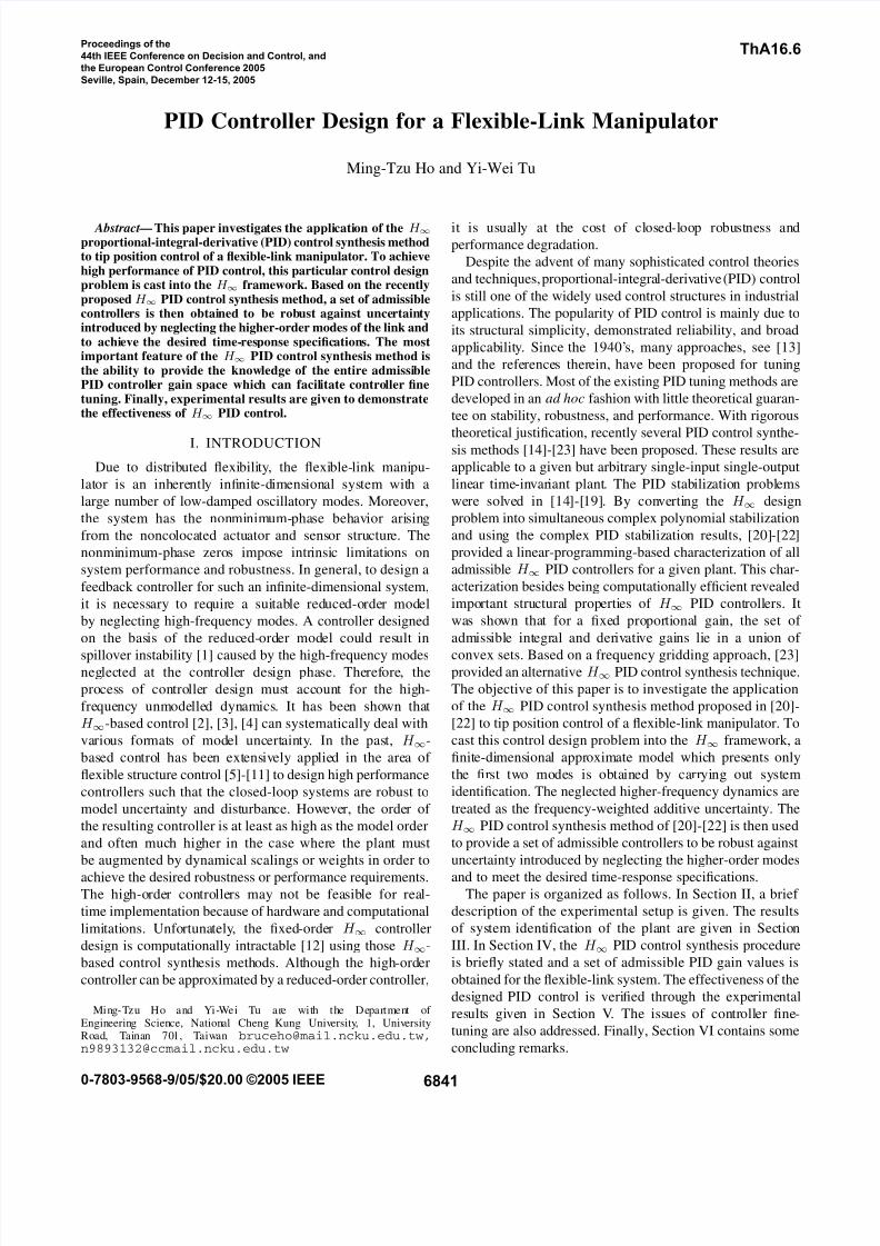
II. DESCRIPTION OF EXPERIMENTAL SETUP

An experimental single-link flexible manipulator has been

constructed as shown by the schematic diagram in Fig. 1.

The flexible link is a rectangular stainless-steel bar (304)

AmplifierUnit

MotorDriver

DCMotor

Encoder

A/D Converter

D/A Converter

Encoder

DSP Board

TMS320F240 EVM

Ultrasonic Sensor ReceiverUltrasonic Sensor Transmitter

Hub Flexible Link

Fig. 1. Schematic diagram of the experimental setup.

with 34.5-cm length, 3-cm width, and 0.045-cm thickness.

The link is coupled to a permanent magnet DC motor by a

hub. The transmitter of an ultrasonic sensor is mounted atthe free end tip of the link and its receiver is fixed on top

of the hub. This ultrasonic sensor is used to measure the tip

deflection of the link. The transmitter of the ultrasonic sensor

also acts as a payload. An optical encoder with resolution

1000 pulses/rev attached to the shaft of the DC motor is used

to measure the angular position of the shaft. The controller

is implemented on a DSP board, EVM320F240 Evaluation

Module manufactured by Spectrum Digital, Inc. This board is

based on the Texas Instruments TMS320F240 digital signal

processor (20 MHz/16-bit). A voltage signal is generated

according to the designed control law and is also supplied

to a motor driver which drives the DC motor. A voltage

amplifier is used to interface with the DSP board and theultrasonic sensor. The flexible link has a circular motion in

the horizontal plane. Due to flexibility of the link, the open-

loop response of the tip motion has significant oscillation.

The aim of this paper is to design a PID controller to position

the tip of the link to a set point as fast as possible with the

desired level of vibration suppression.

III. SYSTEM IDENTIFICATION AND UNCERTAINTY

DESCRIPTION

The flexible link is a distributed-parameter system that

can be described by an infinite-dimensional mathemati-

cal model. Control design methods often require excessive

computational time, if they are applied to such a high-complexity model. In practice, the reduced-order model is

used to conform to computational limitations. In this section,

system identification is exploited to construct a reduced-

order model of the system with an associated bound on the

model mismatch from the actual system by means of the

measurements of the response from the actual system. This

reduced-order model and its uncertainty bound can then be

used for controller synthesis.A theoretical model of the link has been first derived based

on the finite element method. Combining the derived model

of the link and the theoretical model of the DC motor, an

infinite-dimensional theoretical model of the voltage input

of the motor to the tip angular position of the link is

obtained. Although the theoretical model is impossible to

exactly characterize the dynamical behavior of the system, it

provides valuable a priori knowledge about this system. It is

shown that the energy of the vibration modes is essentially

dominated by the first two modes. Thus, for control purpose,

it is adequate to use a model covering the first two modes.

From the theoretical model, we know that the second vibra-

tion mode is located at 175.69013 rad/sec. A sampling rate

at 500 Hz is adequate for the identification experiments. The

input signal for system identification is a 0.1-200 Hz pseudo-

random noise. To avoid aliasing, an eighth-order low-pass

Butterworth filter is used with a cut-off frequency of 200

Hz. The time-domain input and output pairs are collected

and then transformed into the frequency domain by using the

fast Fourier transform. The leakage problem is minimized by

using the Hamming window. The parameters of the transfer

function model are obtained from least-squares estimation.

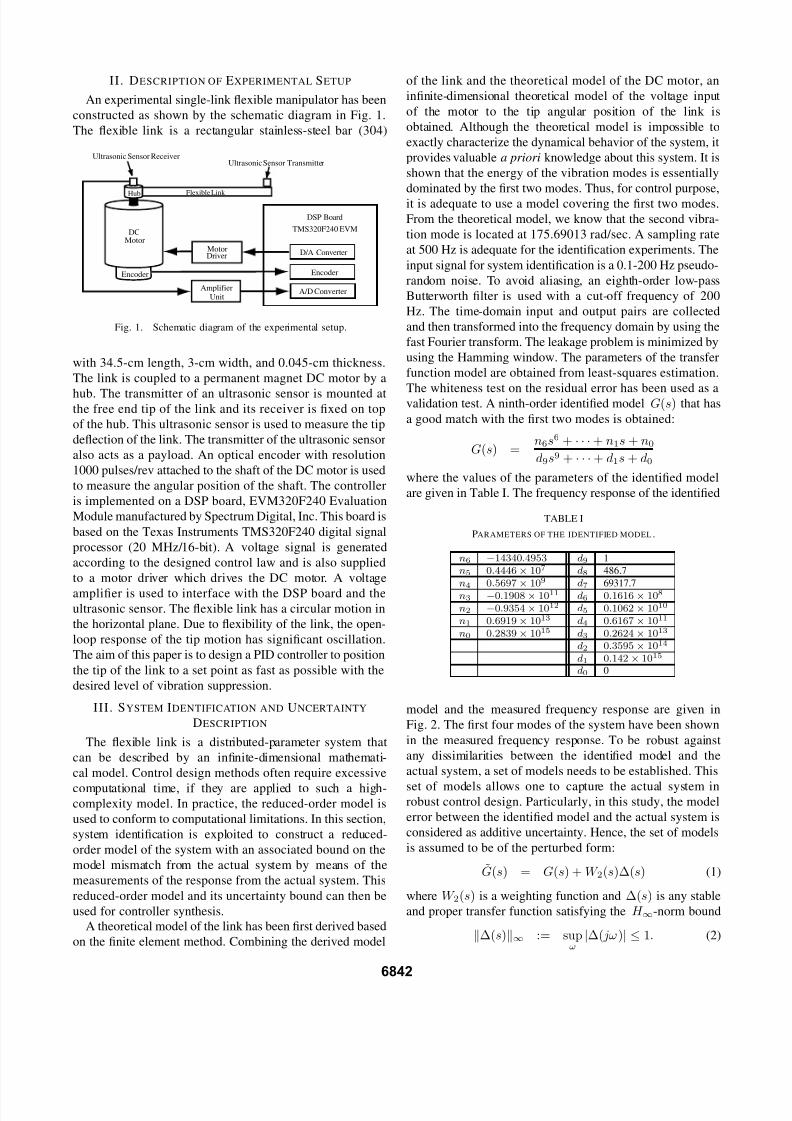
The whiteness test on the residual error has been used as avalidation test. A ninth-order identified model G(s) that has

a good match with the first two modes is obtained:

G(s) =n6s6 + · · · + n1s + n0

d9s9 + · · · + d1s + d0

where the values of the parameters of the identified model

are given in Table I. The frequency response of the identified

TABLE I

PARAMETERS OF THE IDENTIFIED MODEL .

n6 −14340.4953 d9 1

n5 0.4446 × 107 d8 486.7

n4 0.5697 × 109 d7 69317.7

n3 −0.1908 × 1011 d6 0.1616 × 108

n2 −0.9354 × 1012 d5 0.1062 × 1010

n1 0.6919 × 1013 d4 0.6167 × 1011

n0 0.2839 × 1015 d3 0.2624 × 1013

d2 0.3595 × 1014

d1 0.142 × 1015

d0 0

model and the measured frequency response are given in

Fig. 2. The first four modes of the system have been shown

in the measured frequency response. To be robust against

any dissimilarities between the identified model and the

actual system, a set of models needs to be established. This

set of models allows one to capture the actual system inrobust control design. Particularly, in this study, the model

error between the identified model and the actual system is

considered as additive uncertainty. Hence, the set of models

is assumed to be of the perturbed form:

G(s) = G(s) + W 2(s)∆(s) (1)

where W 2(s) is a weighting function and ∆(s) is any stable

and proper transfer function satisfying the H ∞-norm bound

∆(s)∞ := supω

|∆( jω )| ≤ 1. (2)

6842

7/30/2019 7B59AA60d01


100

101

102

103

−120

−100

−80

−60

−40

−20

0

20

Frequency (rad/sec)

M a g n i t u d e ( d B )

100

101

102

103

−1000

−800

−600

−400

−200

0

Frequency (rad/sec)

P h a s e ( d e g )

Fig. 2. Bode plots of the measured frequency domain data (−·) and G(s)(−).

The actual system is assumed to reside in˜

G(s). From (1)and (2), it gives that

|G( jω) − G( jω )| ≤ |W 2( jω )|.

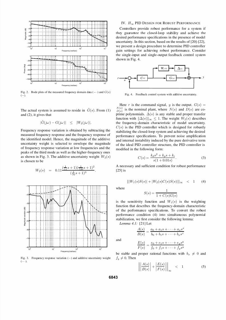
Frequency response variation is obtained by subtracting the

measured frequency response and the frequency response of

the identified model. Hence, the magnitude of the additive

uncertainty weight is selected to envelope the magnitude

of frequency response variation at low frequencies and the

peaks of the third mode as well as the higher-frequency ones

as shown in Fig. 3. The additive uncertainty weight W 2(s)is chosen to be

W 2(s) = 0.11 (111s + 1)(

1720s + 1)

2

( 170s + 1)3

.

100

101

102

103

−80

−70

−60

−50

−40

−30

−20

−10

Frequency (rad/sec)

M a

g n i t u d e v a r i a t i o n ( d B )

Fig. 3. Frequency response variation (−) and additive uncertainty weight(−·).

IV. H ∞ PID DESIGN FOR ROBUST PERFORMANCE

Controllers provide robust performance for a system if

they guarantee the closed-loop stability and achieve the

desired performance specifications in the presence of model

uncertainty. In this section, based on the results of [20]-[22],

we present a design procedure to determine PID controller

gain settings for achieving robust performance. Consider

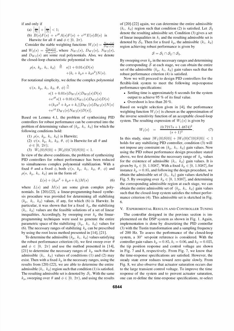
the single-input and single-output feedback control systemshown in Fig. 4.

_

C (s)

(s)W (s)2 ∆

G (s)+

r y

Fig. 4. Feedback control system with additive uncertainty.

Here r is the command signal, y is the output. G(s) =N (s)

D(s)

is the nominal plant, where N (s) and D(s) are co-

prime polynomials. ∆(s) is any stable and proper transfer

function with ∆(s)∞ ≤ 1. The weight W 2(s) describes

the frequency-domain characteristic of model uncertainty.

C (s) is the PID controller which is designed for robustly

stabilizing the closed-loop system and achieving the desired

performance specifications. To prevent noise amplification

and internal instability induced by the pure derivative term

of the ideal PID controller structure, the PID controller is

modified in the following form:

C (s) =kds2 + k ps + ki

s(1 + 0.01s). (3)

A necessary and sufficient condition for robust performance

[25] is

|W 1(s)S (s)| + |W 2(s)C (s)S (s)|∞ < 1 (4)

where

S (s) =1

1 + C (s)G(s)

is the sensitivity function and W 1(s) is the weighting

function that describes the frequency-domain characteristic

of the performance specifications. To convert the robust

performance condition (4) into simultaneous polynomial

stabilization, we first consider the following lemma:

Lemma 4.1: [21] LetA(s)

B(s)=

a0 + a1s + · · · + axsx

b0 + b1s + · · · + bxsx

andE (s)

F (s)=

e0 + e1s + · · · + eysy

f 0 + f 1s + · · · + f ysy

be stable and proper rational functions with bx = 0 and

f y = 0. Then

A(s)

B(s)

+

E (s)

F (s)

∞

< 1 (5)

6843

7/30/2019 7B59AA60d01


if and only if

(a)a0b0

+

e0f 0

< 1;

(b) B(s)F (s) + ejθA(s)F (s) + ejφE (s)B(s) is

Hurwitz for all θ and φ ∈ [0, 2π).

Consider the stable weighting functions W 1(s) =N W 1(s)DW 1(s)

and W 2(s) =N W 2(s)DW 2(s)

, where N W 1(s), DW 1(s), N W 2(s),

and DW 2(s) are some real polynomials. Also, we denote

the closed-loop characteristic polynomial to be

ρ(s, k p, ki, kd)∆= s(1 + 0.01s)D(s)

+(ki + k ps + kds2)N (s).

For notational simplicity, we define the complex polynomial

ψ(s, k p, ki, kd, θ, φ)∆=

s(1 + 0.01s)DW 1(s)DW 2(s)D(s)

+ejθs(1 + 0.01s)N W 1(s)DW 2(s)D(s)

+(kds2 + k ps + ki)[DW 1(s)DW 2(s)N (s)

+ejφDW 1(s)N W 2(s)D(s)].

Based on Lemma 4.1, the problem of synthesizing PIDcontrollers for robust performance can be converted into the

problem of determining values of (k p, ki, kd) for which the

following conditions hold:

(1) ρ(s, k p, ki, kd) is Hurwitz;

(2) ψ(s, k p, ki, kd, θ, φ) is Hurwitz for all θ and

φ ∈ [0, 2π);

(3) |W 1(0)S (0)| + |W 2(0)C (0)S (0)| < 1.

In view of the above conditions, the problem of synthesizing

PID controllers for robust performance has been reduced

to simultaneous complex polynomial stabilization. With a

fixed θ and a fixed φ, both ψ(s, k p, ki, kd, θ , φ) and

ρ(s, k p, ki, kd) are in the form of:

L(s) + (kds2 + k ps + ki)M (s) (6)

where L(s) and M (s) are some given complex poly-

nomials. In [20]-[22], a linear-programming-based synthe-

sis procedure was provided for determining all stabilizing

(k p, ki, kd) values, if any, for which (6) is Hurwitz. In

particular, it was shown that for a fixed k p, the stabilizing

(ki, kd) values are the feasible solutions of a set of linear

inequalities. Accordingly, by sweeping over k p the linear-

programming techniques were used to generate the entire

parametric space of the stabilizing (k p, ki, kd) values for

(6). The necessary ranges of stabilizing k p can be prescribed

by using the root locus method presented in [14], [21].To determine the admissible (k p, ki, kd) values satisfying

the robust performance criterion (4), we first sweep over θ

and φ ∈ [0, 2π) and use the method presented in [14],

[21] to determine the necessary ranges of k p such that the

admissible (ki, kd) values of conditions (1) and (2) may

exist. Then with a fixed k p in the necessary ranges, using the

results from [20]-[22], we are able to determine the entire

admissible (ki, kd) region such that condition (1) is satisfied.

The resulting admissible set is denoted by S 1. With the same

k p, sweeping over θ and φ ∈ [0, 2π), and using the results

of [20]-[22] again, we can determine the entire admissible

(ki, kd) region such that condition (2) is satisfied. Let S 2denote the resulting admissible set. Condition (3) gives a set

of linear inequalities in ki and the resulting admissible set is

denoted by S 3. Then for a fixed k p, the admissible (ki, kd)region achieving robust performance is given by

S = S 1 ∩ S 2 ∩ S 3.

By sweeping over k p in the necessary ranges and determining

the corresponding S at each stage, we can obtain the entire

set of the admissible (k p, ki, kd) gain values such that the

robust performance criterion (4) is satisfied.

Now we will proceed to design PID controllers for the

flexible-link system to meet the following step-response

performance specifications:

• Settling time is approximately 6 seconds for the system

output to achieve 95 % of its final value.

• Overshoot is less than 20 %.

Based on weight selection given in [4], the performance

weighting function W 1(s) is chosen as the approximation of

the inverse sensitivity function of an acceptable closed-loopsystem. The resulting expression of W 1(s) is given by

W 1(s) =(0.7217s + 1.4874)2

(s + 1)2. (7)

In this study, since |W 1(0)S (0)| + |W 2(0)C (0)S (0)| < 1holds for any stabilizing PID controller, condition (3) will

not impose any constraint on (k p, ki, kd) gain values. Now

using the PID robust performance design procedure stated

above, we first determine the necessary range of k p values

for the existence of admissible (ki, kd) gain values. It is

given by k p ∈ [0, 1.9387]. With a fixed k p ∈ [0, 1.9387], for

instance k p = 0.85, and following the design procedure, we

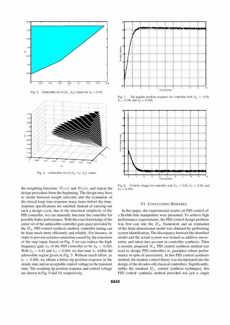
obtain the admissible set of (ki, kd) gain values sketched inFig. 5. By sweeping over k p ∈ [0, 1.9387], and determining

the corresponding admissible region at each stage, we can

obtain the entire admissible set of (k p, ki, kd) gain values

such that the closed-loop system satisfies the robust perfor-

mance criterion (4). This admissible set is sketched in Fig.

6.

V. EXPERIMENTAL RESULTS AND CONTROLLER TUNING

The controller designed in the previous section is im-

plemented on the DSP system as shown in Fig. 1. Again,

implementation is done by discretizing the PID controller

(3) with the Tustin transformation and a sampling frequency

of 200 Hz. To assess the performance of the closed-loopsystem, a 30◦ set-point reference is considered. With the

controller gain values k p = 0.85, ki = 0.06, and kd = 0.025,

the tip position response and control voltage are shown

in Fig. 7 and 8, respectively. From Fig. 7, we know that

the time-response specifications are satisfied. However, the

steady state error reduces toward zero quite slowly. From

Fig. 8, we also observe that actuator saturation occurs due

to the large transient control voltage. To improve the time

response of the system and to prevent actuator saturation,

one can re-define the time-response specifications, re-select

6844

7/30/2019 7B59AA60d01


0 0.02 0.04 0.06 0.08 0.1 0.12 0.14 0.160

0.005

0.01

0.015

0.02

0.025

0.03

0.035

ki

k d

Fig. 5. Admissible set of (ki, kd) values for kp = 0.85.

0

0.1

0.20 0.005 0.01 0.015 0.02 0.025 0.03 0.035

0.65

0.7

0.75

0.8

0.85

0.9

0.95

1

1.05

1.1

1.15

kd

ki

k p

Fig. 6. Admissible set of (kp, ki, kd) values.

the weighting functions W 1(s) and W 2(s), and repeat the

design procedure from the beginning. The design may have

to iterate between weight selection and the evaluation of

the closed-loop time response many times before the time-

response specifications are satisfied. Instead of carrying out

such a design cycle, due to the structural simplicity of the

PID controller, we can manually fine-tune the controller for

possibly better performance. With the exact knowledge of the

entire set of the admissible controller gain space provided by

the H ∞ PID control synthesis method, controller tuning canbe done much more efficiently and reliably. For instance, in

order to prevent actuator saturation caused by the transition

of the step input, based on Fig. 5 we can reduce the high

frequency gain kd of the PID controller to be kd = 0.008.

With k p = 0.85 and kd = 0.008, we fine-tune ki within the

admissible region given in Fig. 5. Without much effort, as

ki = 0.006, we obtain a better tip position response in the

steady state and an acceptable control voltage in the transient

state. The resulting tip position response and control voltage

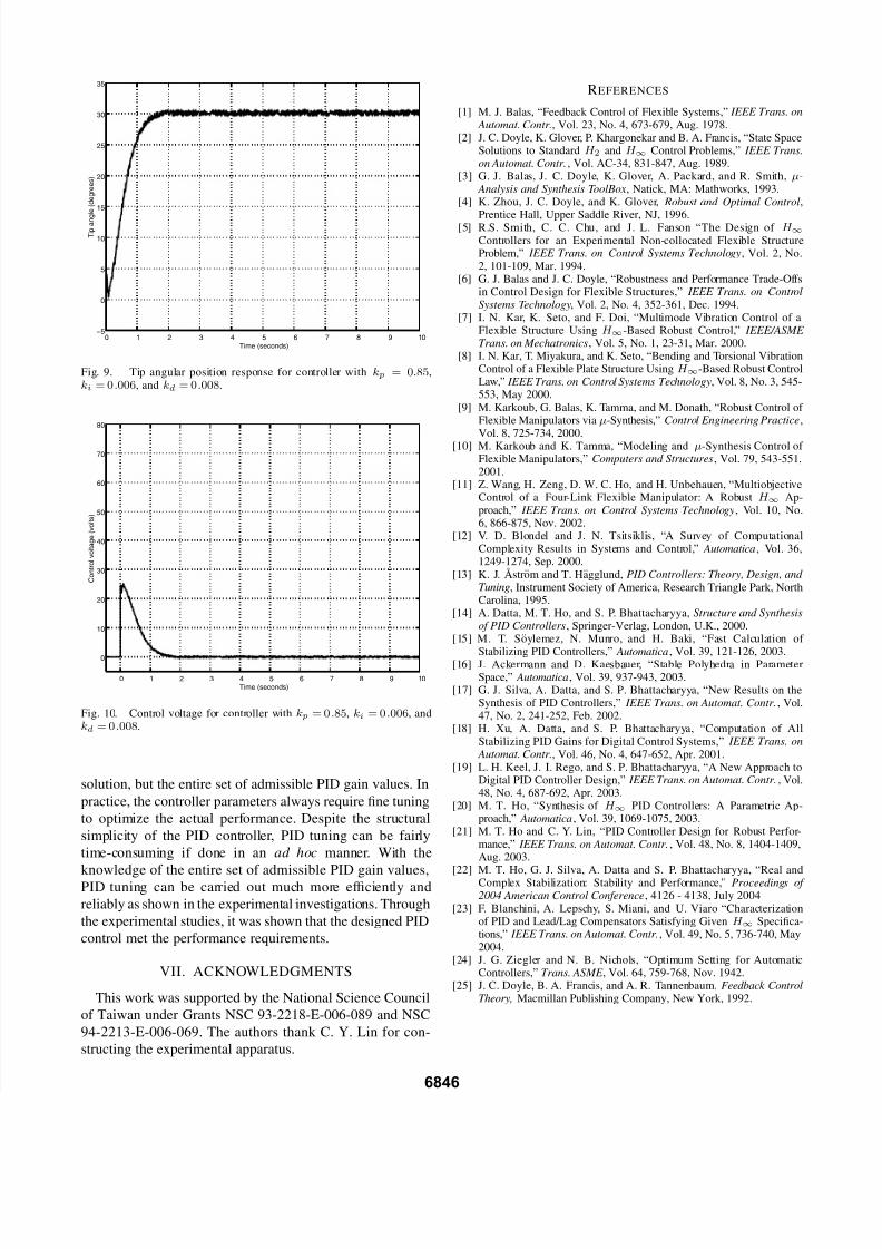
are shown in Fig. 9 and 10, respectively.

0 1 2 3 4 5 6 7 8 9 105

0

5

10

15

20

25

30

35

Time (seconds)

T i p

a n g l e

( d e g r e e s )

Fig. 7. Tip angular position response for controller with kp = 0.85,ki = 0.06, and kd = 0.025.

0 1 2 3 4 5 6 7 8 9 10

0

10

20

30

40

50

60

70

80

Time (seconds)

C o n t r o l v o l t a g e ( v o l t s )

Fig. 8. Control voltage for controller with kp = 0.85, ki = 0.06, andkd = 0.025.

VI. CONCLUDING REMARKS

In this paper, the experimental results on PID control of

a flexible-link manipulator were presented. To achieve high

performance requirements, the PID control design problem

was first cast into the H ∞ framework and an estimation

of the finite-dimensional model was obtained by performingsystem identification. The discrepancy between the identified

model and the actual system was treated as additive uncer-

tainty and taken into account in controller synthesis. Then

a recently proposed H ∞ PID control synthesis method was

used to design PID controllers to guarantee robust perfor-

mance in spite of uncertainty. In this PID control synthesis

method, the modern control theory was incorporated into the

design of the decades-old classical controllers. Significantly,

unlike the standard H ∞ control synthesis techniques, this

PID control synthesis method provided not just a single

6845

7/30/2019 7B59AA60d01


0 1 2 3 4 5 6 7 8 9 10−5

0

5

10

15

20

25

30

35

Time (seconds)

T i p a n g l e ( d e g r e e s )

Fig. 9. Tip angular position response for controller with kp = 0.85,ki = 0.006, and kd = 0.008.

0 1 2 3 4 5 6 7 8 9 10

0

10

20

30

40

50

60

70

80

Time (seconds)

C o n t r o l v o l t a g e ( v o l t s )

Fig. 10. Control voltage for controller with kp = 0 .85, ki = 0.006, andkd = 0.008.

solution, but the entire set of admissible PID gain values. In

practice, the controller parameters always require fine tuning

to optimize the actual performance. Despite the structural

simplicity of the PID controller, PID tuning can be fairly

time-consuming if done in an ad hoc manner. With the

knowledge of the entire set of admissible PID gain values,PID tuning can be carried out much more efficiently and

reliably as shown in the experimental investigations. Through

the experimental studies, it was shown that the designed PID

control met the performance requirements.

VII. ACKNOWLEDGMENTS

This work was supported by the National Science Council

of Taiwan under Grants NSC 93-2218-E-006-089 and NSC

94-2213-E-006-069. The authors thank C. Y. Lin for con-

structing the experimental apparatus.

REFERENCES

[1] M. J. Balas, “Feedback Control of Flexible Systems,” IEEE Trans. on

Automat. Contr., Vol. 23, No. 4, 673-679, Aug. 1978.[2] J. C. Doyle, K. Glover, P. Khargonekar and B. A. Francis, “State Space

Solutions to Standard H 2 and H ∞ Control Problems,” IEEE Trans.on Automat. Contr., Vol. AC-34, 831-847, Aug. 1989.

[3] G. J. Balas, J. C. Doyle, K. Glover, A. Packard, and R. Smith, µ- Analysis and Synthesis ToolBox , Natick, MA: Mathworks, 1993.

[4] K. Zhou, J. C. Doyle, and K. Glover, Robust and Optimal Control,

Prentice Hall, Upper Saddle River, NJ, 1996.[5] R.S. Smith, C. C. Chu, and J. L. Fanson “The Design of H ∞Controllers for an Experimental Non-collocated Flexible StructureProblem,” IEEE Trans. on Control Systems Technology, Vol. 2, No.2, 101-109, Mar. 1994.

[6] G. J. Balas and J. C. Doyle, “Robustness and Performance Trade-Offsin Control Design for Flexible Structures,” IEEE Trans. on Control

Systems Technology, Vol. 2, No. 4, 352-361, Dec. 1994.[7] I. N. Kar, K. Seto, and F. Doi, “Multimode Vibration Control of a

Flexible Structure Using H ∞-Based Robust Control,” IEEE/ASME Trans. on Mechatronics, Vol. 5, No. 1, 23-31, Mar. 2000.

[8] I. N. Kar, T. Miyakura, and K. Seto, “Bending and Torsional VibrationControl of a Flexible Plate Structure Using H ∞-Based Robust ControlLaw,” IEEE Trans. on Control Systems Technology, Vol. 8, No. 3, 545-553, May 2000.

[9] M. Karkoub, G. Balas, K. Tamma, and M. Donath, “Robust Control of Flexible Manipulators via µ-Synthesis,” Control Engineering Practice,

Vol. 8, 725-734, 2000.[10] M. Karkoub and K. Tamma, “Modeling and µ-Synthesis Control of Flexible Manipulators,” Computers and Structures, Vol. 79, 543-551,2001.

[11] Z. Wang, H. Zeng, D. W. C. Ho, and H. Unbehauen, “MultiobjectiveControl of a Four-Link Flexible Manipulator: A Robust H ∞ Ap-proach,” IEEE Trans. on Control Systems Technology, Vol. 10, No.6, 866-875, Nov. 2002.

[12] V. D. Blondel and J. N. Tsitsiklis, “A Survey of ComputationalComplexity Results in Systems and Control,” Automatica, Vol. 36,1249-1274, Sep. 2000.

[13] K. J. Astrom and T. Hagglund, PID Controllers: Theory, Design, and Tuning, Instrument Society of America, Research Triangle Park, NorthCarolina, 1995.

[14] A. Datta, M. T. Ho, and S. P. Bhattacharyya, Structure and Synthesisof PID Controllers, Springer-Verlag, London, U.K., 2000.

[15] M. T. Soylemez, N. Munro, and H. Baki, “Fast Calculation of

Stabilizing PID Controllers,” Automatica, Vol. 39, 121-126, 2003.[16] J. Ackermann and D. Kaesbauer, “Stable Polyhedra in ParameterSpace,” Automatica, Vol. 39, 937-943, 2003.

[17] G. J. Silva, A. Datta, and S. P. Bhattacharyya, “New Results on theSynthesis of PID Controllers,” IEEE Trans. on Automat. Contr., Vol.47, No. 2, 241-252, Feb. 2002.

[18] H. Xu, A. Datta, and S. P. Bhattacharyya, “Computation of AllStabilizing PID Gains for Digital Control Systems,” IEEE Trans. on

Automat. Contr., Vol. 46, No. 4, 647-652, Apr. 2001.[19] L. H. Keel, J. I. Rego, and S. P. Bhattacharyya, “A New Approach to

Digital PID Controller Design,” IEEE Trans. on Automat. Contr., Vol.48, No. 4, 687-692, Apr. 2003.

[20] M. T. Ho, “Synthesis of H ∞ PID Controllers: A Parametric Ap-proach,” Automatica, Vol. 39, 1069-1075, 2003.

[21] M. T. Ho and C. Y. Lin, “PID Controller Design for Robust Perfor-mance,” IEEE Trans. on Automat. Contr., Vol. 48, No. 8, 1404-1409,Aug. 2003.

[22] M. T. Ho, G. J. Silva, A. Datta and S. P. Bhattacharyya, “Real andComplex Stabilization: Stability and Performance,” Proceedings of 2004 American Control Conference, 4126 - 4138, July 2004

[23] F. Blanchini, A. Lepschy, S. Miani, and U. Viaro “Characterizationof PID and Lead/Lag Compensators Satisfying Given H ∞ Specifica-tions,” IEEE Trans. on Automat. Contr., Vol. 49, No. 5, 736-740, May2004.

[24] J. G. Ziegler and N. B. Nichols, “Optimum Setting for AutomaticControllers,” Trans. ASME , Vol. 64, 759-768, Nov. 1942.

[25] J. C. Doyle, B. A. Francis, and A. R. Tannenbaum, Feedback ControlTheory, Macmillan Publishing Company, New York, 1992.

6846

Documents

7B59AA60d01