3,350+OPEN ACCESS BOOKS

108,000+INTERNATIONAL

AUTHORS AND EDITORS115+ MILLION

DOWNLOADS

BOOKSDELIVERED TO

151 COUNTRIES

AUTHORS AMONG

TOP 1%MOST CITED SCIENTIST

12.2%AUTHORS AND EDITORS

FROM TOP 500 UNIVERSITIES

Selection of our books indexed in theBook Citation Index in Web of Science™

Core Collection (BKCI)

Chapter from the book Aerial VehiclesDownloaded from: http://www.intechopen.com/books/aerial_vehicles

PUBLISHED BY

World's largest Science,Technology & Medicine

Open Access book publisher

Interested in publishing with IntechOpen?Contact us at book.department@intechopen.com

29

An Evasive Maneuvering Algorithm for UAVs in Sense-and-Avoid Situations

David Hyunchul Shim KAIST

South Korea

1. Introduction

Highly autonomous unmanned aerial vehicles (UAVs) will need advanced flight management systems that will actively sense the surrounding environment and make a series of intelligent decisions to accomplish the given mission with minimum intervention from remotely located human operators. In near future, it is expected that UAVs will be found as a ubiquitous surrogate for manned vehicles in such fields as airborne sensing, payload delivery, and ultimately aerial combat. In that process, UAVs must be integrated into civilian or military airspaces along with other manned and unmanned aerial vehicles. However, such level of autonomy is yet to be fully developed. Reportedly, a German tactical UAV named LUNA had a close encounter with an Afghan Airline A300B4 in the sky over Kabul, Afghanistan on August 30, 2004. Attributed to a failure of the nearby air traffic control tower to follow standard procedures, two vehicles occupied the same airspace at the same time, no farther than 50 meters when closest. The UAV operator managed to command an evasive maneuver just a split second before impact. The strong wake of A300B4 blew the UAV into an unrecovered dive as seen by the onboard video system in Fig. 1. As exemplified in this rare but alarming event, the collision avoidance has to be incorporated into the flight management system especially when the vehicle is flying in a crowded airspace or at low altitudes where many obstacles such as terrain and buildings pose threat to safe flight.

Figure 1. A near-miss incident of a UAV and A300 airplane (August 2004)

There are also increasingly many occasions that UAVs have to fly at a lower altitude where they are not free from collisions from obstacles such as terrain, buildings or power lines. In order for a UAV to avoid any imminent collision with other vehicles or such obstacles, it should be capable of sensing and tracking of objects, collision prediction, dynamic path planning and tracking. When the trajectories of objects on potential collision courses are predicted, a collision-free trajectory should be computed in real-time. There are a number of

A300

www.intechopen.com

Aerial Vehicles

622

research results for real-time path planning (Bellingham et al, 2003; Dunbar et al, 2002; Milam et al, 2002). In the context of emergency evasive maneuver, however, one would expect that the vehicle may need to maneuver at its full dynamic capability, i.e., maximum turn rate, acceleration/deceleration, or climb/descent. In such cases, the inputs to control surfaces may saturate or the vehicle states, such as roll angle or cruise velocity, may reach the acceptable limits. In order to compute a plausible trajectory that the vehicle can actually fly along without exceeding its dynamic range, a proposed method should be capable of taking such limits into account when computing an evasion trajectory. In this article, we introduce a nonlinear model predictive control (NMPC) based approach, which can be applied to nonlinear dynamic systems with state constraints and input saturation, unlike most control theories available as now. One drawback of MPC is, as often pointed out, the heavy numerical load, which is now considered well within the reach of the latest CPU technology as demonstrated in (Shim & Sastry, 2006). In this article, we present an MPC-based collision avoidance algorithm for safe trajectory generation and control of constrained nonlinear dynamic system with input saturation in real-time. We also introduce an active sensing method using a laser scanner. We consider a number of scenarios with moving vehicles or obstacles in the surroundings. The proposed approach is validated by a series of realistic simulations and experiments including a head-on collision and a flight in an urban canyon.

2. Real-time evasive Maneuvering using Model Predictive Control

In this section, we present the formulation of an NMPC-based approach for real-time safe trajectory generation during an evasive maneuver for avoiding collision. We consider scenarios that, when a UAV flies to a given destination, a collision with nearby flying or stationary obstacles are anticipated. The position information of obstacles is assumed to be directly measured or available from other sources including active communication with cooperating agents or an eye-in- the-sky.

2.1 NMPC Formulation

Suppose we are given a nonlinear time-invariant dynamic system such that

( 1) ( ( ), ( ))x k f x k u k+ = (1)

( ) ( ( ))y k g x k= (2)

where ∈ ⊂ ∈ ⊂,x un nx X u U .{ { The optimal control input sequence over the finite receding

horizon N is obtained by solving the following nonlinear programming problem:

Find *( ), ,..., 1u k k i i N= + − such that (3)

*( ) arg min ( , , )u k V x k u=

where

1

( , , ) ( ( ), ( )) ( ( ))k N

i k

V x k u L x i u i F x k N+ −

=

= + +∑ (4)

www.intechopen.com

An Evasive Maneuvering Algorithm for UAVs in Sense-and-Avoid Situations

623

where ( , ),L x u is a positive definite cost function and F is the terminal cost. Herein, *( ),u k ,..., 1k i i N= + − is the optimal control sequence that minimizes ( , , )V x k u such that * *( , ) ( , , ( , )) ( , , )V x k V x k u x k V x k u= ≤ , ( )u k U∀ ∈ . The cost function term L is chosen as

( ) ( )1

1 1( , ) ( ) ( , )

2 2

onTr r T

ll

L x u x x Q x x u Ru S x P x η=

= − − + + +∑ (5)

The first term penalizes the deviation from the original course. The second term penalizes

the control input. ( )S x is the term that penalizes any states not in X as suggested in (Shim et

al, 2003). Finally, ( , )v lP x η is to implement the collision avoidance capability in this NMPC

framework: ( , )v lP x η is a function that monotonically increases as 2|| || 0η− →v lx , where

3

vx ∈{ is the position of the vehicle and ηl is the coordinates or l-th out of total on

obstacles being simultaneously tracked. The control input saturation can be facilitated by enforcing

max max

min min( )

⎧ >⎪= ⎨

<⎪⎩i i i

i

i i i

u if u uu k

u if u u (6)

during optimization. In this manner, one can find the control input sequence that will be always within the physical limit of the given dynamic system. We employ the optimization method based on indirect method of Lagrangian multiplier suggested in (Sutton & Bitmead, 2000).

Vehicle Dynamics

MPC supervisor

MPC Optimization Path planner

-

Navigation

Sensors

Figure 2. Flight control system architecture with MPC and explicit feedback loop

When an optimal control sequence is found at each epoch k, the control law is given as

( )* *( ) ( ) ( ) ( )u k u k K y k y k= + − (7)

where K is a explicit feedback control gain, which can be found by approaches such as in

(Shim, 2000). With *( ),u k ,..., 1k i i N= + − , one can find *( )y k by solving recursively the

given nonlinear dynamics with 0( ) ( )x i x i= as the initial condition. Ideally, if the dynamic

model used in the prediction in the optimization problem is identical to the actual dynamics and there is no disturbance, the plant would behave as predicted. In the real world, such assumptions cannot be justified due to the inevitable model mismatch, disturbance, and

www.intechopen.com

Aerial Vehicles

624

many other reality factors satisfied. Therefore, with a tracking feedback controller in the feedback loop, the system can track the given trajectory reliably in the presence of disturbance or modeling error. The architecture of the proposed flight control system is given in Fig. 2.

2.2 Obstacle Sensing

For effective collision avoidance, it is very important to detect the location of obstacles of concern in an accurate and timely manner. Such information can be supplied by a preloaded map or information sent by other cooperative neighboring vehicles. However, such information may not be accurate, up-to-date, or always available if communication is lost. A local sensing is favored since it can provide up-to-second information. Obstacle detection can be done using active or passive sensors such as radar, laser scanners, or mono or stereo cameras and the choice depends on many factors such as operating condition, accuracy, and detection range. The laser scanning computes the distance to an object by measuring the time of flight (TOF) of the laser beam to make a round trip from the source to the reflected point on an object. The operation is straightforward and the measurement is very accurate, so it is suitable for short-range detection. However, as the detection range depends on the intensity of the light that radiates from the laser source, the range is limited by the maximum allowable intensity of the beam. Active radar has similar attributes since it operates in a similar principle. The resolution of radar sensing depends on the wavelength of radio wave used. Recently gigahertz-range radars are often used for its more accurate imaging capability at the expense of shorter detection range. Active sensing may not be desired when a covert operation is required. Camera-based detection is attractive as it is a passive detection and the imaging device is usually much cheaper and smaller than comparable radar or laser sensors. However, cameras do not directly give the ranging information. A stereo camera system may be used to measure the distance by the parallax, but it is useful only when the objects are close enough. Optic flow can be also used for short-range detection (Rydergard, 2004; Hrabar, 2005). For long-range detection, the pixel area occupied by the obstacle can be the only visual cue to sense the existence and range. The resulted accuracy is usually much lower than the active sensing methods mentioned above. In this article, we choose to use a laser scanner for obstacle sensing. A laser ranging sensor consists of a laser source, a photo-receptor and a rotating mirror for planar scanning. An accurate timing device measures the time lapse from the moment the laser beam is emitted to the moment the laser beam reflected on an object returns to the receptor. A rotating mirror reflects the laser beam in a circular plane, allowing for two-dimensional scanning. At each scan, the sensor reports a set of measurements that supplies the following measurement set:

{ }( , ), 1,...,L n n measY d n Nβ= = (8)

where ,n nd β and measN represent the distance from an object, the angle in the scanning

plane, and the total number of measurements per scan, respectively. Each measurement, i.e., the relative distance from the laser scanner to a scanned point in the laser-scanner coordinate system, can be written into a vector form such that

( )/ | cos sinL L LD L n n n nd β β= +X i j (9)

www.intechopen.com

An Evasive Maneuvering Algorithm for UAVs in Sense-and-Avoid Situations

625

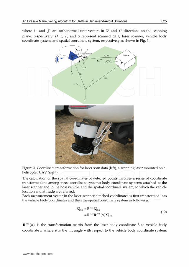
where Li and Lj are orthonormal unit vectors in XL and YL directions on the scanning

plane, respectively. D, L, B, and S represent scanned data, laser scanner, vehicle body coordinate system, and spatial coordinate system, respectively as shown in Fig. 3.

obstacle

SZ

SX

SY

/D LX1 1

( , )i id β+ +

( , )i id βlaser scanner

S

BX

BX

LX

LZ

BY

BZ

/L BX

LY

α

S

DX

Figure 3. Coordinate transformation for laser scan data (left), a scanning laser mounted on a helicopter UAV (right)

The calculation of the spatial coordinates of detected points involves a series of coordinate transformations among three coordinate systems: body coordinate systems attached to the laser scanner and to the host vehicle, and the spatial coordinate system, to which the vehicle location and attitude are referred. Each measurement vector in the laser scanner-attached coordinates is first transformed into the vehicle body coordinates and then the spatial coordinate system as following:

// /

/ //( )

S S L LD L D L

S B B L LD Lα

=

=

X R X

R R X (10)

/ ( )B L αR is the transformation matrix from the laser body coordinate L to vehicle body

coordinate B where α is the tilt angle with respect to the vehicle body coordinate system.

www.intechopen.com

Aerial Vehicles

626

/S BR denotes the transformation matrix from vehicle body coordinates to spatial coordinates. Finally, the spatial coordinate of the obstacle is found by:

/ /

/ / // /( )

S S S SD D L L B B

S B B L L S B B SD L L B Bα

= + +

= + +

X X X X

R R X R X X (11)

Using (11), one can find the spatial coordinate of sampled points on obstacles by combining the raw measurement vector with the position, heading, and attitude of the vehicle, which are available from the onboard navigation system of the UAV. It should be noted that the detection accuracy in the spatial coordinate system not only depends on the laser scanner’s accuracy itself, but also on the accuracy of the vehicle states. To ensure conflict-free navigation in an airspace filled with obstacles, the laser scanner should scan the surroundings wide enough to find conflict-free trajectory. For example, if the laser scanner is installed to scan the area horizontally, an actuation in the pitch axis is necessary so that the scanner can cover the frontal area sufficiently higher than the rotor disc plane and lower than the landing gear. Fig. 3 shows an actuated laser scanner mounted on a helicopter UAV (Shim et al, 2006). The scanner is mounted on a tilt actuator with an

encoder, which provides the tilt angle α in / ( )B L αR . Fig. 4 shows visualizations of laser scan

data, which is obtained by (11). As can be seen, the shapes of objects can be accurately detected and reconstructed.

Figure 4. Point cloud of obstacles sensed by a laser scanner shown in Fig. 3 (left: scanning of ground-based objects of area shown in the inset image; right: scanning of a UAV airborne)

2.3 Trajectory Generation

For collision avoidance, we choose ( , )v lP x η in (5) such that

1

( , )( ) ( )

v l Tv l v l

P xx G x

ηη η ε

=− − +

(11)

where G is positive definite and 0ε > is to prevent ill conditioning when 2

0.vx η− → One

can choose { , , },x y zG diag g g g= 0ig > for an orthogonal penalty function. The penalty

function (11) serves as a repelling field and has nonzero value for entire state space even

power lines

trees

Host UAVpower pole

www.intechopen.com

An Evasive Maneuvering Algorithm for UAVs in Sense-and-Avoid Situations

627

when the vehicle is far enough from obstacles. The crucial difference from the potential field approach here is that we optimize over a finite receding horizon, not only for the current time as in the potential field approach. For obstacle avoidance, we consider two types of scenarios: 1) a situation when the vehicle needs to stay as far as possible from the obstacles even if no direct collision is anticipated and 2) a situation when the vehicle can be arbitrarily close to the obstacle as long as no direct conflict is caused. For the second situation, (11) can

be enacted only when min2vx η σ− → , where minσ is the minimum safety distance from

other vehicles. Since MPC algorithms optimize over the receding finite horizon into future, the predicted

obstacles’ trajectory over ,..., 1k i i N= + − is needed in (11). It is anticipated that the inclusion

of predicted obstacle locations in the optimization will produce more efficient evasion trajectory if the prediction is reasonably accurate. If the obstacle detection system is capable of estimating the current velocity in addition to the position of an obstacle, one can

predict ( )l kη by extrapolating it over Np steps, namely prediction Horizon, using an equation

such that

( ) ( ) ( )( 1)l l lk i k tv k iη η+ = + Δ − (12)

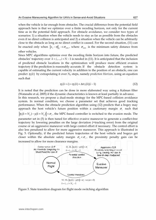
It is noted that the prediction can be done in more elaborated way using a Kalman filter (Watanabe et al, 2005) if the dynamic characteristics is known at least partially in advance. In this research, we propose a dual-mode strategy for the MPC-based collision avoidance system. In normal condition, we choose a parameter set that achieves good tracking performance. When the obstacle prediction algorithm using (12) predicts that a bogey may

approach the host vehicle’s future position within a cautionary margin cσ such that

( ) ( )l p p ck N y k Nη σ+ − + < , the MPC-based controller is switched to the evasion mode. The

parameter set in (5) is then tuned for effective evasive maneuver to generate a conflict-free trajectory by lowering penalties on the large deviation (=tracking error) from the original course or an aggressive maneuver with large control effort if necessary. The control effort is also less penalized to allow for more aggressive maneuver. This approach is illustrated in Fig. 5. Optionally, if the predicted future trajectories of the host vehicle and bogeys get

closer within the absolute safety margin a cσ σ< , the proximity penalty gain can be

increased to allow for more clearance margins.

, , ( ) ( )

,... 1

l c

p

l k k y k

k i i N

η σ∃ ∃ − <

= + −

, , ( ) ( ) ,( 0)

,... 1

l c

p

l k k y k

k i i N

η σ α α∀ ∀ − > + >

= + −

Figure 5. State transition diagram for flight mode switching algorithm

www.intechopen.com

Aerial Vehicles

628

In the following section, we apply the proposed MPC algorithm for (a) one vehicle versus a non-cooperating vehicle and (b) one vehicle in an environment with obstacles.

3. Simulation and experiment results

3.1 One on One Situation

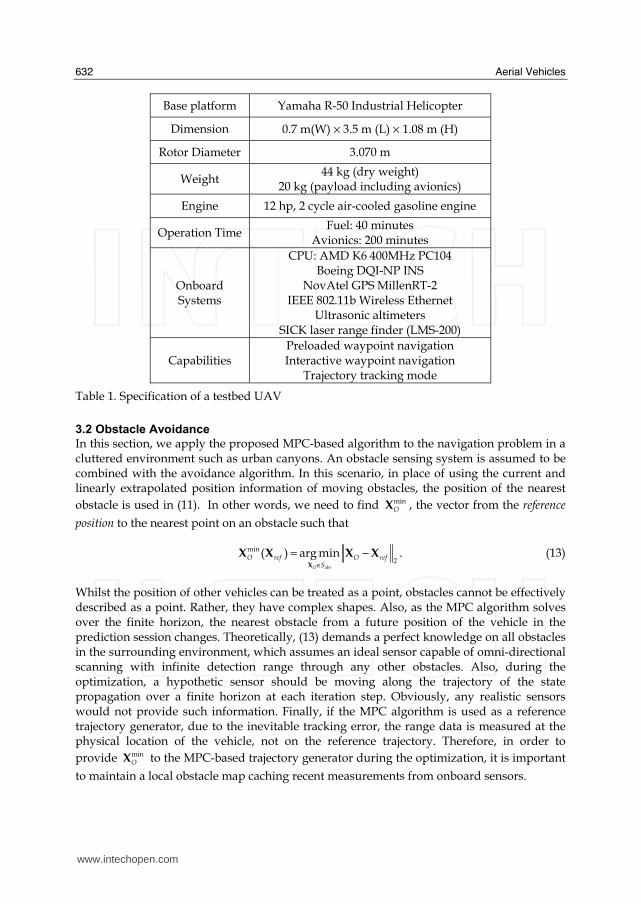
In this scenario, we consider a UAV cruising at 3m/s at 10 meters above the ground. Without loss of generality, we use a dynamic model for a rotorcraft UAV based on Yamaha R-50 industrial helicopter (Shim, 2000), whose specification is given in Table 1. The bogeys are staged to moves along a straight line at a constant altitude and speed at various incident angles. The detection range is simulated to be 50 meters based on a typical laser scanner and 100 meters for a hypothetic vision-based system. We investigate a fraction of these combinations of the factors mentioned above, which would highlight the performance of the proposed approach so that we may have the insight to the behavioral patterns and characteristics of the algorithm with a realistic detection. In this scenario, we consider the case when a UAV encounters a bogey at various speed and incident angle. The horizon N is set to 100 with 40 ms of sampling time, so the prediction horizon spans over 4 seconds. For fixed obstacles, stationary obstacles 12 meters away can be considered in the optimization when cruising at 3 m/s. As expected, the moving obstacles will impose more challenges in detection and finding a safe evasion trajectory in a short time. First, we consider the following cases: a bogey cruising towards the UAV at 2 m/s, 5 m/s,

15 m/s and 30m/s. The cautionary margin 50cσ = m and the absolute safety margin

10aσ = m. We judge the vehicles collide when the distance from each other is less than 5 m.

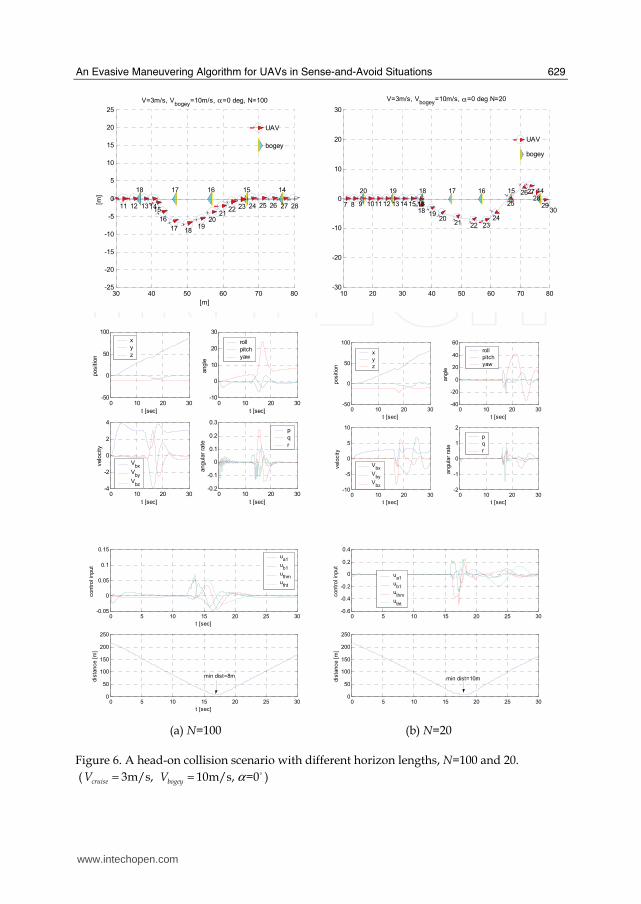
In Fig. 6, an example when a bogey closes in at 10 m/s, with 0° incident angle (head-on

collision). As can be seen in the figures, the host UAV maintains sufficient margin, which

decreases as low as 8 m/s, well above the minimal distance. For comparison, we consider

when the horizon N is much shorter to demonstrate the advantage of the receding horizon

approach. The simulation result when N is shortened to 20 (=0.8sec) and all other

parameters are fixed as before is given in Fig. 5 as well. The result shows that the UAV

manages to escape the collision, but the vehicle goes into a violent transient motion during

the close fly-by interval. It is attributed that the short horizon length does not allow a

sufficient time to predict the collision and then steer the vehicle away from the collision

course. We also note the heading of the vehicle is implicitly determined by the optimization.

In the following examples, we consider a set of different approach velocities and incident

angles.

In Fig. 7, a number of approach velocities are tested. In Fig. 7-(d), the vehicle passes the bogey with 7m distance, which is considered as a bare minimum. It is expected that a longer horizon length will help to avoid the obstacle with a more sufficient margin. In Fig. 8, the trajectory planner shows a reliable performance in computing safe trajectories when the bogey flies in at various incident angles. In overall, the MPC-based collision avoidance algorithm demonstrates a satisfactory performance in various scenarios.

www.intechopen.com

An Evasive Maneuvering Algorithm for UAVs in Sense-and-Avoid Situations

629

30 40 50 60 70 80-25

-20

-15

-10

-5

0

5

10

15

20

25

2827

14

26

bogey

UAV

2524

15

232221

20

16

[m]

V=3m/s, Vbogey

=10m/s, α=0 deg, N=100

1918

17

17

16

151413

18

1211

[m]

10 20 30 40 50 60 70 80-30

-20

-10

0

10

20

30

3029

1428

27

bogey

UAV

2615

25

2423

16

2221

17

V=3m/s, Vbogey

=10m/s, α=0 deg N=20

2019

18

181716151413

19

121110

20

987

0 10 20 30-50

0

50

100

t [sec]

positio

n

x

y

z

0 10 20 30-10

0

10

20

30

t [sec]

angle

roll

pitch

yaw

0 10 20 30-4

-2

0

2

4

t [sec]

velo

city

Vbx

Vby

Vbz

0 10 20 30-0.2

-0.1

0

0.1

0.2

0.3

t [sec]

angula

r ra

te

p

q

r

0 10 20 30-50

0

50

100

t [sec]

positio

n

x

y

z

0 10 20 30-40

-20

0

20

40

60

t [sec]

angle

roll

pitch

yaw

0 10 20 30-10

-5

0

5

10

t [sec]

velo

city

Vbx

Vby

Vbz

0 10 20 30-2

-1

0

1

2

t [sec]

angula

r ra

te

p

q

r

0 5 10 15 20 25 30-0.05

0

0.05

0.1

0.15

t [sec]

contr

ol in

put

ua1

ub1

uthm

utht

0 5 10 15 20 25 300

50

100

150

200

250

t [sec]

dis

tance [

m]

min dist=8m

0 5 10 15 20 25 30-0.6

-0.4

-0.2

0

0.2

0.4

contr

ol in

put

ua1

ub1

uthm

utht

0 5 10 15 20 25 300

50

100

150

200

250

dis

tance [

m]

min dist=10m

(a) N=100 (b) N=20 Figure 6. A head-on collision scenario with different horizon lengths, N=100 and 20.

( 3m/s,cruiseV = 10m/s, =0bogeyV α= c )

www.intechopen.com

Aerial Vehicles

630

10 20 30 40 50 60 70 80-20

-15

-10

-5

0

5

10

15

20

1

29

23

28

4

27

56

26

7

25

89

24

10

23

11

22

12

21

1314

20

1516

19

1718

18

19

17

20

16

21

1514

22

13

2324

12

25

11

2627

10

28

9

2930

87654

10 20 30 40 50 60 70 80-20

-15

-10

-5

0

5

10

15

20

28

11

27

12

2625

13

2423

14

2221

15

20

16

1918

17

17

18

16

1514

19

1312

20

1110

21

9

22

87

23

6

24

5

(a) 2 m/scruiseV = (b) 5m/scruiseV =

10 20 30 40 50 60 70 80-20

-15

-10

-5

0

5

10

15

20

3292827

15

262524232221

16

2019

1817

17

161514131211

18

109876

19

5432

(c) 15m/scruiseV = (d) 30m/scruiseV =

Figure 7. Various cruise velocity 2,5,15,30m/scruiseV = of host vehicle with 10m/sbogeyV =

10 20 30 40 50 60 70 80-20

-15

-10

-5

0

5

10

15

20

2827262524

19

2322

18

2120

1719

1817

16

1615

1413

15

1211

14

109

13

8765

10 20 30 40 50 60 70 80-20

-15

-10

-5

0

5

10

15

20

272625242322212019

18

17

16

15

18171615141312111098765

(a) =45α c (b) =90α c

10 20 30 40 50 60 70 80-20

-15

-10

-5

0

5

10

15

20

2827262524

19

2322

18

2120

17

191817

16

16

1514

13

15

12111098765

10 20 30 40 50 60 70 80-20

-15

-10

-5

0

5

10

15

20

30

20

292827

19

26252423

18

2221

2019

1817

17

1615

16

141312

15

11109

14

876

13

543

12

2

(c) =135α c (d) =180α c

Figure 8. Various incident angles =45 ,90 ,135 ,180 ,α c c c c 3m/scruiseV = with 10m/sbogeyV =

www.intechopen.com

An Evasive Maneuvering Algorithm for UAVs in Sense-and-Avoid Situations

631

In order to validate the proposed algorithm experimentally, two helicopter UAVs (Table 1) are deployed in a collision course (Fig. 9 and 10). Two vehicles are initially flown manually 30 meters apart and commanded to trade their position while flying at 1.2 m/s. Then the MPC algorithm running on a notebook computer with Pentium 1.8 GHz CPU computes safe trajectories for each vehicle in MATLAB/Simulink environment. At each sampling time of 100 ms, each vehicle communicates with the centralized trajectory planner but not directly each other over a wireless channel to report the current position and receive a new waypoint. The experiment was performed in four separate occasions and the vehicles could fly to their own destination while avoiding collision. An experiment result set is shown in Fig. 10. It can be seen that the separation in the middle was about 12 meters from center to center of the vehicles and less than 9 meters from tip-to-tip.

Figure 9. Mid-air collision avoidance between two rotorcraft UAVs using real-time MPC

Figure 10. Trajectories of two UAVs Experiment result of Trajectories of of dynamic path planning for collision avoidance

www.intechopen.com

Aerial Vehicles

632

Base platform Yamaha R-50 Industrial Helicopter

Dimension 0.7 m(W) × 3.5 m (L) × 1.08 m (H)

Rotor Diameter 3.070 m

Weight 44 kg (dry weight)

20 kg (payload including avionics)

Engine 12 hp, 2 cycle air-cooled gasoline engine

Operation TimeFuel: 40 minutes

Avionics: 200 minutes

Onboard Systems

CPU: AMD K6 400MHz PC104 Boeing DQI-NP INS

NovAtel GPS MillenRT-2 IEEE 802.11b Wireless Ethernet

Ultrasonic altimeters SICK laser range finder (LMS-200)

Capabilities Preloaded waypoint navigation Interactive waypoint navigation

Trajectory tracking mode

Table 1. Specification of a testbed UAV

3.2 Obstacle Avoidance

In this section, we apply the proposed MPC-based algorithm to the navigation problem in a cluttered environment such as urban canyons. An obstacle sensing system is assumed to be combined with the avoidance algorithm. In this scenario, in place of using the current and linearly extrapolated position information of moving obstacles, the position of the nearest

obstacle is used in (11). In other words, we need to find minOX , the vector from the reference

position to the nearest point on an obstacle such that

min

2( ) arg min .

O obs

O ref O refS∈

= −X

X X X X (13)

Whilst the position of other vehicles can be treated as a point, obstacles cannot be effectively described as a point. Rather, they have complex shapes. Also, as the MPC algorithm solves over the finite horizon, the nearest obstacle from a future position of the vehicle in the prediction session changes. Theoretically, (13) demands a perfect knowledge on all obstacles in the surrounding environment, which assumes an ideal sensor capable of omni-directional scanning with infinite detection range through any other obstacles. Also, during the optimization, a hypothetic sensor should be moving along the trajectory of the state propagation over a finite horizon at each iteration step. Obviously, any realistic sensors would not provide such information. Finally, if the MPC algorithm is used as a reference trajectory generator, due to the inevitable tracking error, the range data is measured at the physical location of the vehicle, not on the reference trajectory. Therefore, in order to

provide minOX to the MPC-based trajectory generator during the optimization, it is important

to maintain a local obstacle map caching recent measurements from onboard sensors.

www.intechopen.com

An Evasive Maneuvering Algorithm for UAVs in Sense-and-Avoid Situations

633

Vehicle position and attitude

from the BEAR avionics

Raw scan data

from laser

scanner

Filter out

inaccurate

measurements

Convert to

local Cartesian

coordinates

Find the nearest

obstacle point

over future

time horizon

Sort and filter

out small

obstacles/noises

Find NC points

closest to

the vehicle

Figure 11. Finding nearest points at each state propagation during prediction (left) and local map building method for the nearest-point approach avoidance (right)

At each scan, the sensor provides measN measurements of the scan points from the nearby

obstacles. Due to the imperfect coverage of the surroundings with possible measurement

errors, each measurement set iOX is first filtered, transformed into local Cartesian

coordinates, and cached in the local obstacle map repository. A first-in, first-out (FIFO) buffer is chosen as the data structure for the local map, whose buffer size is determined by the types of obstacles nearby. If the surrounding is known to be static, the buffer size can be as large as the memory and processing overheads permit. On the other hand, a more dynamic environment would require smaller buffer to reduce the chance to detect obstacles that may not exist anymore. In order to solve (13), the measurement set in the FIFO is sorted in ascending order of

2

iO ref−X X for all i

OX in the local obstacle map, where 1 Ci N≤ ≤ . Prior to be registered in the

database, any anomalies such as salt-and-pepper noise should be discarded. Also, the measurements are examined for any small debris, such as grass blades or leaves blown by the downwash of the rotor. Such small-size objects, not being serious threats for safety, are ignored. In order to eliminate these anomalies, we first discard measurements out of minimum and maximum detection range. Then we apply an algorithm that computes a bounding box that contains a series of subsequent points in the FIFO where the distance between the adjacent points in the sorted sequence is less than a predefined length. Then, if the volume of the bounding box is larger than a threshold of becoming a threat, the coordinates of the nearest point in the bounding box is found and used for computing (9). The procedure of the local obstacle map building method proposed above is illustrated in Fig. 11. The proposed obstacle avoidance algorithm was validated in an actual flight test using the same helicopter UAV used in Section 3.1. The experiment design is carefully scrutinized for the safety: it is performed in a field with portable canopies simulating buildings, not with

real ones. The canopies, measuring 3 × 3 × 3 meters each, are arranged as shown in Fig. 11. The distance between one side to the next adjacent side of canopies is set to 10 meters in the north-south direction and 12 meters in the east-west direction so that the UAV with 3.5 meter long fuselage can pass between the canopies with minimal safe clearance, about 3 meters from the rotor tip to the nearby canopy when staying on course. For validation, an MPC engine originally used for the collision avoidance experiment introduced above is modified for urban navigation problem. The MPC engine is augmented

minOX

www.intechopen.com

Aerial Vehicles

634

with the local map builder using the laser range finder’s data. The MPC with the local map building algorithm is implemented in C language for speed and portability. As shown in Fig. 12, the MPC path planner demonstrated its capability to generate a collision-free trajectory based on the original trajectory with intentional overlapping with buildings.

Figure 12. Aerial view of urban navigation experiment (dashed: given straight path, solid: actual flight path of UAV during experiment)

On-board System

Range

Measurements

Laser Range Finder

Ground Computer

Data Display

and Logging

Local

Map Builder

Nearest

Obstacle Info

Range

Measurements

Obstacle-free

Trajectory

Vehicle StatesBEAR

Flight Management

System

Computation

Results

MPC

Path Generator

Figure 13. Overall system structure used in the experiments (left) and a snapshot of three-dimensional rendering during an urban exploration experiment (right)

A number of experiments for urban flight were performed. For obstacle detection, the vehicle is equipped with an LMS-200 from Sick AG, a two-dimensional laser range finder. It has 80 meters of detection range with 10 mm resolution. The scanner’s measurement is sent to the flight computer via RS-232 and then relayed to the ground station running the MPC-based trajectory generator in Simulink. The trajectory generation module on MATLAB/ Simulink and the ground monitoring/commanding software were executed simultaneously on a computer with Pentium 4, 2.4 GHz with 512 MB RAM running Microsoft Windows XP. The laser scanner data is processed following the procedure described above. In Fig. 13, a three-dimensional rendering from the ground station software is presented. The display

shows the location of the UAV, the reference point marker, minOX to a point in the local

obstacle map at that moment, and laser-scanned points as dots. During the experiments, the laser scanner was able to detect the canopies in the line of sight with outstanding accuracy,

www.intechopen.com

An Evasive Maneuvering Algorithm for UAVs in Sense-and-Avoid Situations

635

as well as other natural and artificial objects including buildings, trees and power lines. The processed laser scanned data in a form of local obstacle map is used in the optimization (5). The trajectory is then sent via IEEE 802.11b to the onboard flight management system at 10Hz. The overall system structure used in the experiments is shown in Fig. 13. The tracking layer controls the host vehicle to follow the revised trajectory. In the repeated experiments, the vehicle was able to fly around the obstacles with sufficient accuracy for tracking the obstacle-free trajectory, as shown in Fig. 12(solid line).

4. Conclusion

In this article, we presented a collision avoidance algorithm for UAVs using nonlinear model predictive control. The preview mechanism of receding horizon control is found ideal for such cases when the obstacles are moving. The proposed algorithm was also applied to obstacle avoidance problems, where onboard sensors combined with updated local map was combined with the MPC solver to compute conflict-free trajectories. Both cases are validated first in simulation and then in realistic experiments using helicopter UAVs. In each set of experiments, the proposed NMPC-based algorithms were able to run in real-time for computing conflict-free trajectories. The proposed algorithm will be further extended to vision-based sensing as well as the avoidance problems of fixed-wing UAVs.

5. References

Bellingham, J.; Kuwata, Y., & How, J. (2003). Stable Receding Horizon Trajectory Control for Complex Environments, AIAA Conference on Guidance, Navigation, and Control, Austin, Texas, August 2003.

Dunbar, W. B.; Milam, M. B.; Franz, R. & Murray, R. M. (2002). Model Predictive Control of a Thrust-Vectored Flight Control Experiment, 15th IFAC World Congress on Automatic Control, Barcelona, Spain, July 2002.

Hrabar, S. E.; Corke, P. I.; Sukhatme, G. S.; Usher, K. & Roberts, J. M. (2005) Combined Optic-Flow and Stereo-Based Navigation of Urban Canyons for a UAV, IEEE/RSJ International Conference on Intelligent Robots and Systems, pp. 302-309, Edmonton, Alberta, Canada, August 2005.

Milam, M. B.; Franz, R. & Murray, R. M. (2002). Real-time Constrained Trajectory Generation Applied to a Flight Control Experiment, IFAC World Congress on Automatic Control, Barcelona, Spain, July 2002.

Polak, E. (1997). Optimization: Algorithms and Consistent Approximations, Springer-Verlag, ISBN 0-387-94971-2, New York, USA.

Rydergard, S. (2004), Obstacle Detection in a See-and-Avoid System for Unmanned Aerial Vehicles, Master’s Thesis, Royal Institute of Technology, Stockholm, Sweden.

Shim, D. H. (2000). Hierarchical Control System Synthesis for Rotorcraft- based Unmanned Aerial Vehicles, Ph. D. thesis, University of California, Berkeley, 2000.

Shim, D. H.; Kim, H. J. & Sastry, S. (2003). Decentralized Nonlinear Model Predictive Control of Multiple Flying Robots, IEEE Conference on Decision and Control, Maui, HI, December 2003.

Shim, D. H.; Chung, H. & Sastry, S. (2006). Autonomous Exploration in Unknown Urban Environments for Unmanned Aerial Vehicles, IEEE Robotics and Automation Magazine, vol. 13, September 2006 , pp. 27-33, ISSN1070-9932.

www.intechopen.com

Aerial Vehicles

636

Sutton, G. J. & Bitmead, R. R. (2000). Computational Implementation of NMPC to Nonlinear Submarine, In: Nonlinear Model Predictive Control, volume 26, pp. 461-471, Institution Electrical Engineers, ISBN 0852969848, London, UK.

Watanabe, Y.; Calise, A. J.; Johnson, E. N. & J. H. Evers (2005). Minimum-Effort Guidance for Vision-based Collision Avoidance, AIAA Guidance, Navigation, and Control Conference, San Francisco, California, 2005.

www.intechopen.com

Aerial VehiclesEdited by Thanh Mung Lam

ISBN 978-953-7619-41-1Hard cover, 320 pagesPublisher InTechPublished online 01, January, 2009Published in print edition January, 2009

InTech EuropeUniversity Campus STeP Ri Slavka Krautzeka 83/A 51000 Rijeka, Croatia Phone: +385 (51) 770 447 Fax: +385 (51) 686 166www.intechopen.com

InTech ChinaUnit 405, Office Block, Hotel Equatorial Shanghai No.65, Yan An Road (West), Shanghai, 200040, China

Phone: +86-21-62489820 Fax: +86-21-62489821

This book contains 35 chapters written by experts in developing techniques for making aerial vehicles moreintelligent, more reliable, more flexible in use, and safer in operation.It will also serve as an inspiration forfurther improvement of the design and application of aeral vehicles. The advanced techniques and researchdescribed here may also be applicable to other high-tech areas such as robotics, avionics, vetronics, andspace.

How to referenceIn order to correctly reference this scholarly work, feel free to copy and paste the following:

David Hyunchul Shim (2009). An Evasive Maneuvering Algorithm for UAVs in Sense-and-Avoid Situations,Aerial Vehicles, Thanh Mung Lam (Ed.), ISBN: 978-953-7619-41-1, InTech, Available from:http://www.intechopen.com/books/aerial_vehicles/an_evasive_maneuvering_algorithm_for_uavs_in_sense-and-avoid_situations