748 IEEE TRANSACTIONS ON MOBILE COMPUTING, …guanhua/paper/07084168.pdf · they leverage different time intervals between transmitted symbols to represent information. However, this

TiM: Fine-Grained Rate Adaptation in WLANsGuanhua Wang, Student Member, IEEE, Shanfeng Zhang, Kaishun Wu,Member, IEEE,

Qian Zhang, Fellow, IEEE, and Lionel M. Ni, Fellow, IEEE

Abstract—Channel condition varies frequently in wireless networks. To achieve good performance, devices need rate adaptation. In

rate adaptation, choosing proper modulation schemes based on channel conditions is vital to the transmission performance. However,

due to the natural character of discrete modulation types and continuous varied link conditions, we cannot make a one-to-one mapping

from modulation schemes to channel conditions. This matching gap causes either over-select or under-select modulation schemes

which limits throughput performance. To fill-in the gap, we propose time-line modulation (TiM), a novel three-Dimensional modulation

scheme by adding time dimension into current amplitude-phase domain schemes. With estimation of channel condition, TiM changes

base-band data transmission time by artificially interpolating values between original data points without changing amplitude-phase

domain modulation type. We implemented TiM on USRP2 and conducted comprehensive simulations. Results show that, compared

with rate adaptation choosing from traditional modulation schemes, TiM can improve channel utilization up to 200 percent.

Index Terms—Adapting interpolation rate, modulation scheme, rate adaptation

Ç

1 INTRODUCTION

WIRELESS communication suffers from continuouslyvaried link condition, which leads to packet loss or

bit errors. This time-varying problem is the main issue thatlimits wireless link’s performance. The movement of linknodes and background interference make this time-varyingissue even worse. To achieve good channel utilization insuch severe conditions, sender needs to select the highesttransmission rate that current channel can support, anddynamically adapt the rate to meet with the continuouslyvaried link condition. This procedure is called rate adapta-tion. Given its widely deployment in wireless local areanetworks (WLANs) and mesh networks, rate adaptationplays a vital role in wireless networks.

A large quantity of recent researches advance rateadaptation. Most of them focus on channel condition esti-mation, like signal-to-noise ratio (SNR) [1], [2], [3], biterror rate (BER) [4], [5]. Based on the channel conditionthey estimate, they pick up the corresponding modula-tion scheme for proper transmission rate. Recent litera-ture can estimate channel condition with high accuracyand to some extent, make relatively full use of existedmodulation schemes. However, none of them everfocuses on whether existed modulation schemes wechoose from are good enough. So here raises a naturalquestion, “can we push the limit of rate adaptation by

modifying modulation schemes we choose from and getmore throughput gain?”

Properly choosing modulation schemes is a crucial issuein rate adaptation. This choosing process can be regarded asa procedure of mapping different modulation schemes tovaried channel conditions. Since the value (e.g., SNR) repre-sents channel condition is continuous whereas modulationtypes are discrete, we cannot make a perfect one-to-onematching from modulation schemes to channel conditions.Because of this non-perfect matching, we may under-selector over-select a scheme that cannot use the bandwidth effi-ciently. We evaluate the residual between the scheme canutilize and the current channel condition can really support.This link margin is significantly large (details in Section2.3). Given this modulation gap, we can revise current mod-ulation schemes to move a step forward of rate adaptationand get better channel utilization.

In this paper, we propose a novel modulation schemeTime-line Modulation (TiM), to fix with the non-perfectmatching problem. The widely used modulation schemes inWLANs are designed mainly in amplitude-phase domain,such as binary phase shift keying (BPSK), quadrature phaseshift keying (QPSK), 16-QAM (Quadrature AmplitudeModulation) and 64-QAM. Based on this two dimension(2D) scheme, TiM adds time dimension to make it into 3D.As depicted in Fig. 1, in the traditional 16-QAMmodulationscheme, it only has shift in amplitude and phase. The greenline refers to the phase shift value whereas the blue linestands for amplitude value. TiM adds time domain as thetransmission time of one data symbol, namely Ts, which isshown in Fig. 1 as the red arrow. This 2D to 3D expansioncan allow us to insert modulation schemes between twoexisted adjacent schemes (e.g., QPSK and 16-QAM) on timedomain without changing anything on traditional ampli-tude-phase domain.

Some articles also propose to leverage time-domaindiversity in modulation [6], [7]. All of them are using timedomain diversity to convey information. More precisely,

� G. Wang and K. Wu are with Guangdong Province Key Laboratory ofPopular High Performance Computers, College of Computer Science andSoftware Engineering, Shenzhen University and Hong Kong University ofScience and Technology. E-mail: {gwangab, kwinson}@ust.hk.

� S. Zhang and Q. Zhang are with Department of Computer Science andEngineering, Hong Kong University of Science and Technology.E-mail: {szhangai, qianzh}@cse.ust.hk.

� L. Ni is with the Department of Computer and Information Science,University of Macau. E-mail: [email protected].

Manuscript received 8 Apr. 2014; revised 17 Mar. 2015; accepted 3 Apr. 2015.Date of publication 10 Apr. 2015; date of current version 2 Feb. 2016.For information on obtaining reprints of this article, please send e-mail to:[email protected], and reference the Digital Object Identifier below.Digital Object Identifier no. 10.1109/TMC.2015.2421938

748 IEEE TRANSACTIONS ON MOBILE COMPUTING, VOL. 15, NO. 3, MARCH 2016

1536-1233� 2015 IEEE. Personal use is permitted, but republication/redistribution requires IEEE permission.See http://www.ieee.org/publications_standards/publications/rights/index.html for more information.

they leverage different time intervals between transmittedsymbols to represent information. However, this kind oftime-domain leverage indeed cannot improve signal’s resis-tance to noise and interference. In TiM, the length value intime-domain (i.e., Ts) can be adjusted by adapting the quan-tity of interpolation values that are inserted between realdata points. And the interpolation values can enhance emit-ted signal to be more robust to interference and more likelyto be correctly recovered on the receiver side.

TiM can adjust fine-grained level by regulating the quan-tity of interpolating values between two adjacent samplingdata points. However, how to estimate the fine-grainedlevel is a critical issue. Since with higher fine-grained level,rate adaptation process may change modulation schemesmore frequently and the changing overhead will be higher.On the other hand, more fine-grained level means moreperfect matching of modulation schemes with channel con-ditions which leads to more throughput gain. Here wedesign a Grain Size Estimation scheme to make the trade-offbetween the overhead of changing rate and fine-grainedmodulation gain.

Since changing modulation schemes on TiM’s timedomain will have time delay, how to manage this modula-tion changing overhead is another problem. TiM allows ratechanging more efficiently by integrating a simple but usefullengthen coordinator (LC) module. It leverages processingdelay and rate changing delay to cancel each other andreduce the overhead.

One point needs to be claimed is that adding time-dimension doesn’t mean TiM can achieve real continuousrate adaptation. This is because of two reasons. First, wecannot use a fixed number of bits to represent continuousvalues which are infinite in system design. Second, there isno need to achieve this which has high overhead withoutgetting significant gain. TiM indeed is also a discrete modu-lation scheme.

Another point worth mentioning is that while TiMremains the same radio sampling rate, by interpolation, itchanges the transmission time of signal symbols, andthereby, causing the signal bandwidth changes accordingly.

We have implemented TiM scheme on USRP2 platform[8]. We also conduct extensive simulations on Matlab foranalysing TiM’s performance. The results show that, with-out changing current 2D modulation schemes, by addingtime domain, TiM can achieve up to 200 percent goodputcompared with traditional schemes. For real world wire-less traffic, TiM can achieve channel utilization efficiency

to nearly 160 percent on average. Furthermore, Grain SizeEstimation and lengthen coordinator’s assistance enhancesTiM’s performance. To sum up, this paper’s contributionsare mainly as follows.

� To the best of our knowledge, TiM is the first to pro-pose 3D modulation scheme that leverages timedomain diversity to fill-in the matching gap ofexisted 2D schemes. The primitive is to lengthen thetransmission time of base-band data.

� TiM incorporates lengthen coordinator to reduce ratechanging overhead.

� Grain Size Estimation module is designed for deter-mining TiM’s fine-grained level in wireless link toachieve better channel utilization.

� We implemented TiM on USRP2 and modified phys-ical layer (PHY) preamble to make a hand-shake ofTiM’s interpolation factor between transceivers. Fur-ther, we validate and evaluate TiM’s performance.

The rest of this paper is organized as follows. In section 2,we mainly depicts some related preliminaries, motivation ofTiM, and a general overview of TiM. Section 3 describesTiM’s detailed system architecture. We implement TiM andassistant modules on USRP2 platform in Section 4. We eval-uate TiM’s performance in Section 5. Section 6 reviews therelated work and Section 7 concludes the paper.

2 PRELIMINARIES AND OVERVIEW

This section depicts some related preliminaries, motivationof TiM, and a general overview of TiM. It first providessome background materials about existed modulationschemes and orthogonal frequency division multiplexing(OFDM) primer. Then it delivers the motivation of our TiMapproach. Finally it gives a brief introduction of the keyideas in TiM.

In PHY, the sender modulates a sequence of bits into aPHY symbol. There are three basic modulation types whichare amplitude shift keying (ASK), phase shift keying (PSK)and frequency shift keying (FSK). In commercial use,namely IEEE 802.11 a/g/n, what we use in current wirelesssystem are BPSK, QPSK, 16-QAM and 64-QAM, etc. Thesewidely-used modulation schemes represent the data bits ona 2D plane which is call constellation diagram.

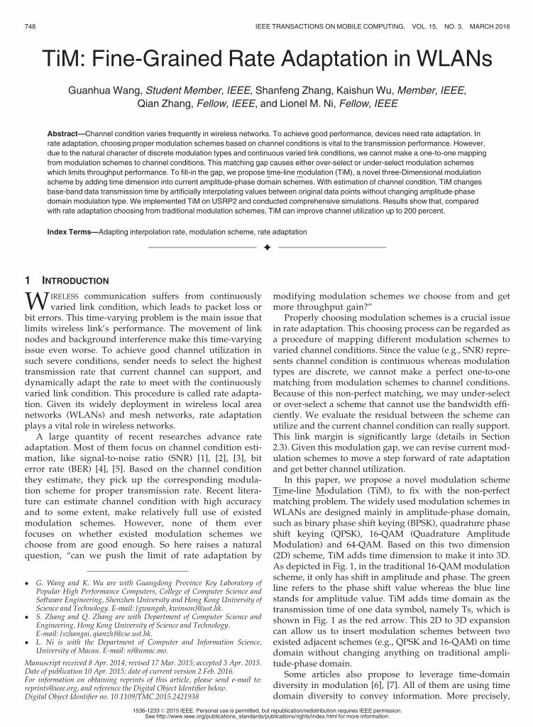
BPSK and QPSK are both leveraging signals’ shifting dif-ference in phase domain. As shown in Fig. 2, BPSK uses 180degree phase shift to define data bit 0 and 1 (e.g., whenphase shift value 0 degree represents bit 0, 180 degree repre-sents bit 1 or vice versa). It is only able to modulate 1 bit (i.e.,b0 in BPSK of Fig. 2) per symbol. However, it has the highestresistance level to noise or distortion. QPSK refers to thatthe signal shifts among the phases states are separated by90 degree, which is depicted in Fig. 2 as QPSK. And eachphase shift state conveys two bits data (i.e., b0b1 in QPSK ofFig. 2), namely 00, 01, 10, 11, respectively. Since two bits aresimultaneously modulated into one symbol, the data trans-mission bitrate of QPSK is twice as that of BPSK.

16-QAM and 64-QAM use both amplitude and phaseshifting to convey more information than either one methodalone. The constellation diagram of 16-QAM is shown inFig. 1 without our time-line dimension (i.e., Ts). In eachquadrant of this diagrams there are four state points with

Fig. 1. An example of modified 16-QAM modulation scheme with TiM’sadditional time dimension.

WANG ET AL.: TIM: FINE-GRAINED RATE ADAPTATION IN WLANS 749

difference in amplitude or phase to distinguish each of them.These 16 state points in the whole diagram convey the bitsinformation from 0000 to 1111. Thus 16-QAM is a 4 bits persymbol modulation scheme. 64-QAM is quite similar with16-QAM, it only dense the points in each quadrant from 4 to16, which can be seen in Fig. 2. And each state represents6 bits per symbol (i.e., b0b1b2b3b4b5 in 64-QAMof Fig. 2). Sincethe state points become denser, the signal’s resistance tointerference or noise is weaker. The data transmitted by thismodulation scheme should be in good channel conditions.

2.1 OFDM Primer

We present the design of TiM based on OFDM which is awidely used technique in WLANs (e.g., IEEE 802.11 a/g/n).OFDM is a multiple subcarriers modulation technique inwireless modulation. It divides the whole bandwidth intoseveral orthogonal subcarriers. Then it spreads data into thelow-speed subcarriers and transmits them in parallel. Incurrent Wi-Fi system, OFDM split a 20 MHz into 64 subcar-riers, and each divided subcarrier has 312.5 KHz [9].

In order to modulate base-band data onto OFDM subcar-rier, we need the modulation schemes to use constellationsymbol to represent data information. Commonly usedmod-ulation schemes are BPSK QPSK and so forth. These constel-lation symbol are transformed into time domain samplesthrough a inverse fast Fourier transform (IFFT) process.

To make fully utilization of frequently varied wirelesschannel condition, Wi-Fi sender employs the techniquecalled rate adaptation. Based on the estimation of channelcondition (e.g., SNR), it pick up the densest constellationscheme and highest coding rate to approaching the optimalthroughput that current link can support. And recentlythere are numerous quantity of paper discussing moresophisticated and near-optimal rate adaptation scheme,which may achieve more accuracy and better performance.

2.2 Motivation: 3D Modulation Scheme WithAdditional Time Dimension

For many years, in information theory, there are basicallythree digital modulation types, namely PSK, ASK and FSK.PSK leverages phase shifting value to convey data, whereas

ASK uses amplitude difference and FSK uses frequencyshifting value. However, in IEEE 802.11 standards [9], basi-cally, the modulation schemes (e.g., BPSK, 16-QAM) are alldesigned in the phase-amplitude two dimensions.

The reason why we do not leverage FSK or frequencydomain schems is because the usage of OFDM. OFDM iswidely deployed in current Wi-Fi communication systemowing to its high efficiency of channel utilization. How-ever, OFDM is not perfect. The shortage is that OFDM isstrict with subcarries’ orthogonality and time synchroniz-ing. If we implement FSK into OFDM, it will decrease thesynchronizing performance in OFDM. Further, Addingfrequency domain modulation types also needs the offsetestimation of doppler effect to be more precise. Because ofthese two main reasons, we cannot use FSK in currentmodulation schemes.

Even though each 2Dmodulation scheme (e.g., BPSK) hasfew coding rate (e.g., 1/2 3/4) options, it cannot achievedecent performance [10]. There aremainly two reasons. First,due to the limited number of pre-defined options, traditional2D scheme cannot achieve varied fine-grained level modula-tion whereas TiM can. Second, TiM indeed can be imple-mented with any coding rate and make each of these optionsbemore fine-grainedwhich enhance the performance.

Because the non-perfect matching between existed mod-ulation schemes and channel conditions, it causes through-put loss when changing modulation schemes. Nevertheless,conventional 2D modulation schemes have been studiedfor many years and have already been perfectly designed.So how can we fill-in the matching gap without modifyingthe well-defined amplitude-phase domain schemes? Addi-tionally, we cannot directly use the frequency domainschemes either.

Given all these concerns and analysis above, the onlyway we can modulate the signal besides amplitude-phase2D domain is to design modulation schemes that leveragethe time domain. This expansion from 2D to 3D is a waythat we can fill-in the matching gap between current 2Dmodulation schemes and channel conditions.

2.3 TiM Modulation Framework

The goal of TiM is to cover the matching gap betweenadjacent modulation schemes with negligible overhead.

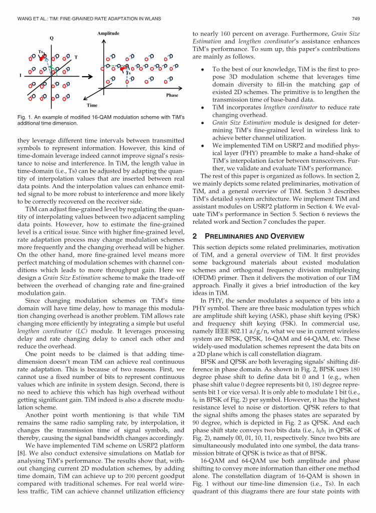
As shown in Table 1, we measured the correspondingSNR threshold on USRP2 [8] platform for different modula-tion schemes with varied coding rates. The SNR thresholdmeasurement is based on packet loss rate. More precisely,when the packet loss rate is above a threshold (empirically

TABLE 1Measurement on SNR Threshold for Different Modulations

Min Required SNR Bitrate Modulation Coding

3 dB 6 Mbps BPSK 1/24 dB 9 Mbps BPSK 3/45.5 dB 12 Mbps QPSK 1/29 dB 18 Mbps QPSK 3/412 dB 24 Mbps 16-QAM 1/217 dB 36 Mbps 16-QAM 3/422 dB 48 Mbps 64-QAM 2/323 dB 54 Mbps 64-QAM 3/4

Fig. 2. Basic 2D modulation schemes: BPSK, QPSK and 64-QAM’s con-stellation diagrams.


30 percent) in a specific transmission bitrate, the senderregards current SNR cannot support this particular trans-mission rate. This measurement is based on fact that rateadaptation algorithm tries its best to minimize the packetloss rate, thus can be conservative [7].

In addition, we do not use the well-designed rate adapta-tion schemes. It is because that using more sophisticatedschemes to measure the channel SNR will increase the mea-surement overhead. However, the measurement in [7] sim-ulates the state-of-the-art rate adaptation scheme, namelySoftRate [11]. Their observation results also support ourlink margin statements.

Based on our experimental results on USRP2 in Table 1,for example, when the estimated channel SNR is in theinterval of minimum SNR requirement of two adjacentmodulation schemes (e.g., 15 dB), choosing either of thesetwo schemes (i.e., 16-QAM with 1/2 coding rate or 16-QAMwith 3/4 coding rate) cannot fully utilize the channel. Andthe residual between selected scheme can utilize and thethroughput that channel can really support is a significantmargin that we want to utilize. By filling in this matchinggap, we can reduce throughput loss of rate changing pro-cess. To this end, we need to ensure that the newly designedmodulation scheme can be inserted exactly between the twotraditional adjacent schemes it based on.

TiM’s insight is to utilize the modulation’s timedomain without disturbing current 2D (amplitude andphase domain) scheme. To do so, trigged by [12], [13]which slowdown clock rate to reduce power consump-tion, we lengthen the data symbol transmission time byadding some interpolating points between adjacent origi-nal data symbols. This interpolation process is easy to beadded in current OFDM modulation procedure and canbe easily implemented on any coding schemes. We realizethis function by modifying the cascaded integrator-comb(CIC) circuits in transceivers.

3 TIM DESIGN

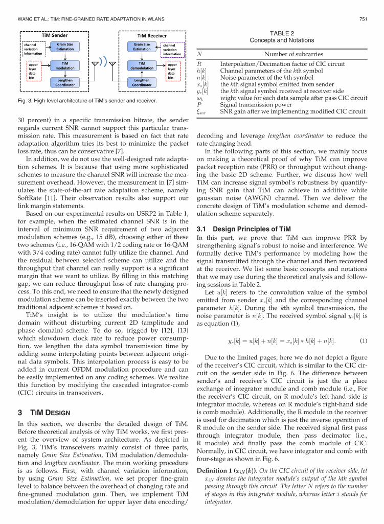
In this section, we describe the detailed design of TiM.Before theoretical analysis of why TiM works, we first pres-ent the overview of system architecture. As depicted inFig. 3, TiM’s transceivers mainly consist of three parts,namely Grain Size Estimation, TiM modulation/demodula-tion and lengthen coordinator. The main working procedureis as follows. First, with channel variation information,by using Grain Size Estimation, we set proper fine-grainlevel to balance between the overhead of changing rate andfine-grained modulation gain. Then, we implement TiMmodulation/demodulation for upper layer data encoding/

decoding and leverage lengthen coordinator to reduce therate changing head.

In the following parts of this section, we mainly focuson making a theoretical proof of why TiM can improvepacket reception rate (PRR) or throughput without chang-ing the basic 2D scheme. Further, we discuss how wellTiM can increase signal symbol’s robustness by quantify-ing SNR gain that TiM can achieve in additive whitegaussian noise (AWGN) channel. Then we deliver theconcrete design of TiM’s modulation scheme and demod-ulation scheme separately.

3.1 Design Principles of TiM

In this part, we prove that TiM can improve PRR bystrengthening signal’s robust to noise and interference. Weformally derive TiM’s performance by modeling how thesignal transmitted through the channel and then recoveredat the receiver. We list some basic concepts and notationsthat we may use during the theoretical analysis and follow-ing sessions in Table 2.

Let u½k� refers to the convolution value of the symbolemitted from sender xs½k� and the corresponding channelparameter h½k�. During the kth symbol transmission, thenoise parameter is n½k�. The received symbol signal yr½k� isas equation (1),

yr½k� ¼ u½k� þ n½k� ¼ xs½k� � h½k� þ n½k�: (1)

Due to the limited pages, here we do not depict a figureof the receiver’s CIC circuit, which is similar to the CIC cir-cuit on the sender side in Fig. 6. The difference betweensender’s and receiver’s CIC circuit is just the a placeexchange of integrator module and comb module (i.e., Forthe receiver’s CIC circuit, on R module’s left-hand side isintegrator module, whereas on R module’s right-hand sideis comb module). Additionally, the R module in the receiveris used for decimation which is just the inverse operation ofR module on the sender side. The received signal first passthrough integrator module, then pass decimator (i.e.,R module) and finally pass the comb module of CIC.Normally, in CIC circuit, we have integrator and comb withfour-stage as shown in Fig. 6.

Definition 1 (xiNðkÞxiNðkÞ). On the CIC circuit of the receiver side, letxiN denotes the integrator module’s output of the kth symbolpassing through this circuit. The letter N refers to the numberof stages in this integrator module, whereas letter i stands forintegrator.

Fig. 3. High-level architecture of TiM’s sender and receiver.

TABLE 2Concepts and Notations

N Number of subcarries

R Interpolation/Decimation factor of CIC circuith½k� Channel parameters of the kth symboln½k� Noise parameter of the kth symbolxs½k� the kth signal symbol emitted from senderyr½k� the kth signal symbol received at receiver sidevk wight value for each data sample after pass CIC circuitP Signal transmission power�snr SNR gain after we implementing modified CIC circuit


Definition 2 (xdðkÞxdðkÞ). Given the output of integrator xiN , the datasymbol need to pass through the decimator (i.e., R module).xdðkÞ denotes the decimator’s output of kth symbol, where drepresents the meaning of decimator.

Definition 3 (ycNðkÞycNðkÞ). Given xiNðkÞ’s definition, here ycNðkÞ isquiet the same. Let ycN denotes the signal output of comb mod-ule. The letterN share the same meaning as in xiNðkÞ, whereasletter c stands for comb. The letter k represents the meaningthat it is the kth symbol passing through this circuit.

Given these definitions above, we first illustrate a sim-ple model, which the receivers CIC filter only contain 1stage of integrator, then decimator and 1 stage of decima-tor. As we have mentioned before, u½k� denotes the emit-ted symbol that received at receiver side with a distortionof h½k�. So after passing the 1 stage integrator, we can getthe output of integrator as equation (2). In equation (2),we can see that the kth symbol also conveys the ðk� 1Þthsymbol’s information, thus make it robust for the receiverto recover the data symbols

xi1ðkÞ ¼ xi1ðk� 1Þ þ uðnÞ ¼Xnk¼0

uðkÞ: (2)

After this 1 stage integrating, the symbol need to passthrough the decimator (i.e., R module). Suppose the deci-mating factor is R, the output of decimator is as equation (3).

xdðmÞ ¼ xi1ðmRÞ ¼XmR

k¼0

uðkÞ: (3)

After that, the signal should pass through 1 stage comb,the output of comb circuit is as equation (4). Thus, after thisprocess, it can get the original data symbols’ information(i.e., uðkÞ) by doing a subtraction between two adjacent deci-mated symbols.

yc1ðmÞ ¼ xdðmÞ � xdðm� 1Þ

¼XmR

k¼0

uðkÞ �Xðm�1ÞR

k¼0

uðkÞ

¼XmR

k¼ðm�1ÞRþ1

uðkÞ:

(4)

The theoretical analysis of one-stage CIC circuit in timedomain is delivered as above. There are mainly three com-ponents in the real four-stage receiver’s CIC circuit. Basedon this simple model mentioned above, we show the realfour-stage CIC circuit’s output by deliver the results of allits three parts separately. The output of the fourth integratoris as equation (5),

xi4ðnÞ ¼Xnk1¼0

Xk1k2¼0

Xk2k3¼0

Xk3k4¼0

½uðk4Þ� (5)

we can get the output of decimator module as equation (6),

xdðmÞ ¼XmR

k1¼0

Xk1k2¼0

Xk2k3¼0

Xk3k4¼0

½uðk4Þ� where m 2 0;n

R

j kh i: (6)

After that, the signal should pass through four-stagecomb module. We can derive the final output of this wholefour-stage CIC circuit as equation (7),

yc4ðmÞ ¼Xðm�3ÞRþ3

k1¼ðm�4ÞRþ4

Xk1þR�1

k2¼k1

Xk2þR�1

k3¼k2

Xk3þR�1

k4¼k3

uðk4Þ: (7)

Given the noise parameter as nðkÞ, the output of noise ynpassing through CIC can be derived from the output of sig-nal passing through CIC as equation (8).

ynðmÞ ¼Xðm�3ÞRþ3

k1¼ðm�4ÞRþ4

Xk1þR�1

k2¼k1

Xk2þR�1

k3¼k2

Xk3þR�1

k4¼k3

nðk4Þ: (8)

Based on the output of CIC circuit (i.e., equation (7)), wecan get that the CIC output is the weighted (i.e., vk) sum ofthe last 4ðR� 1Þ input samples, which can be delivered asthe equation (9),

ysðmÞ ¼XmR

k¼ðm�4ÞRþ4

vkuðkÞ: (9)

Let’s first calculate the SNR of wireless system withoutthe CIC filter procedure. Suppose noise is modeled asAWGN, nðkÞ meets with the Gaussian distribution. Thuswe can derive that,

nðkÞ � Nð0; d2Þ:The SNR (i.e., �0snr) can be represented as equation (10),

where P is the signal transmission power,

�0snr ¼EðuðkÞ � EðuðkÞÞÞ2EðnðkÞ � EðnðkÞÞÞ2 ¼

P

d2: (10)

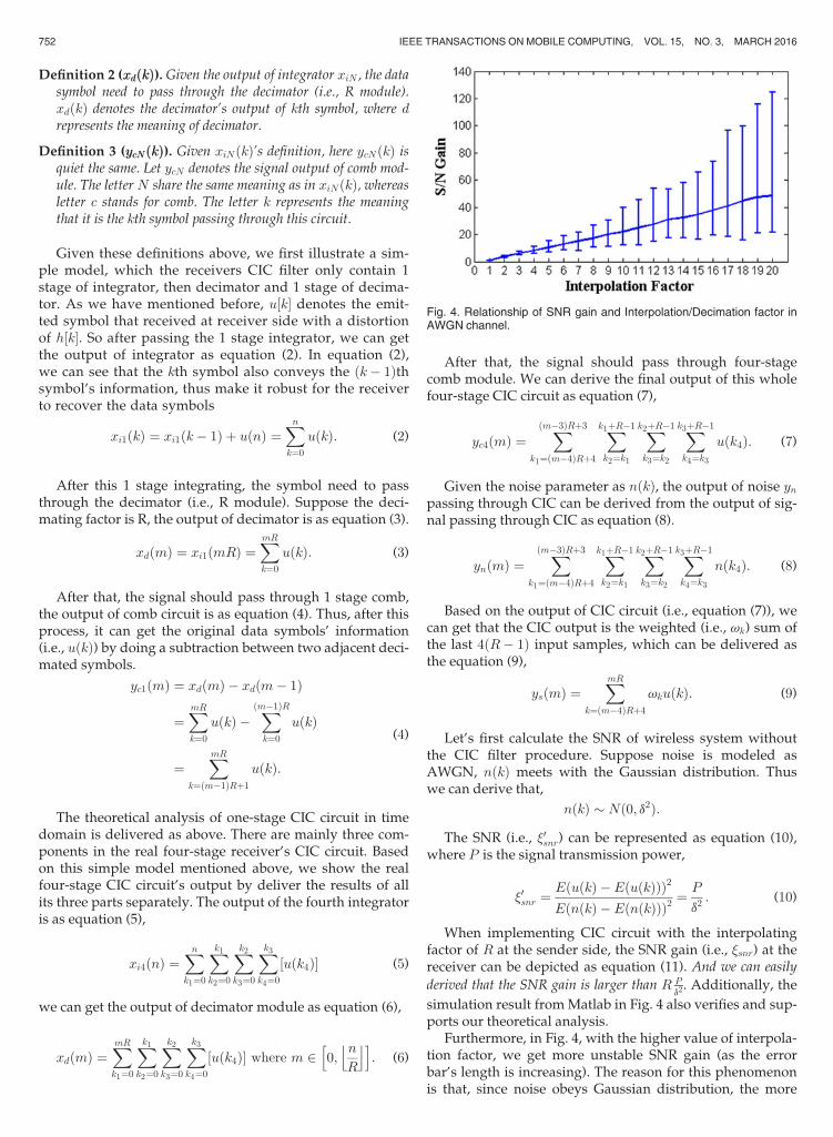
When implementing CIC circuit with the interpolatingfactor of R at the sender side, the SNR gain (i.e., �snr) at thereceiver can be depicted as equation (11). And we can easily

derived that the SNR gain is larger than R Pd2. Additionally, the

simulation result fromMatlab in Fig. 4 also verifies and sup-ports our theoretical analysis.

Furthermore, in Fig. 4, with the higher value of interpola-tion factor, we get more unstable SNR gain (as the errorbar’s length is increasing). The reason for this phenomenonis that, since noise obeys Gaussian distribution, the more

Fig. 4. Relationship of SNR gain and Interpolation/Decimation factor inAWGN channel.


points we collect, the more Gaussian distribution-like thatthe noise will be. However, noise that combined with inter-polation values and real data symbols is independent,whereas the interpolation values and real data symbols arecorrelated. After we leverage the interpolation points tohelp recover the real data points on the receiver side, wethrow them away. Due to noise’s independent attribute,noise information on the interpolation points indeed is lost.Thus it could be less likely of Gaussian distribution. Andthis is the reason for unstable SNR gain we get at high inter-polation/decimation rate.

�snr ¼ Eðy2sðmÞÞEðy2nðmÞÞ

� RPmR

k¼ðm�4ÞRþ4 v2kEðu2ðkÞÞ

d2PmR

k¼ðm�4ÞRþ4 v2k

¼ RP

d2:

(11)

Based on the proof above, we can derive that, TiM’s inter-polating system can help the data signal to be more robust to noiseand interference. The more interpolated values between adja-cent data points, the better recovery of data points at thereceiver side.

3.2 3D Modulation/Demodulation Schemes

To realize TiM, there are several challenges. First, at thesender side, the lengthen process of base band data mustovercome the following difficulties: (1) it must be configura-ble to set different lengthen value during the rate adaptationprocess. (2) how to determine the lengthen value with var-ied channel condition is an open problem. We deliver ourmethods to deal with these two problems from both theoret-ical analysis and Matlab simulation results.

On the receiver side, the design of demodulation schemecan be more challenging. The first issue is the delay ofchanging interpolation/decimation rate between senderand receiver. We present lengthen coordinator to solve thisproblem. Another difficulty is how to recover data pointswith less accurate coordination and synchronizationbetween the sender and the receiver. To handle this prob-lem, we leverage the interpolated points to help improvethe accuracy of data recovery.

3.2.1 Modulation Scheme Design

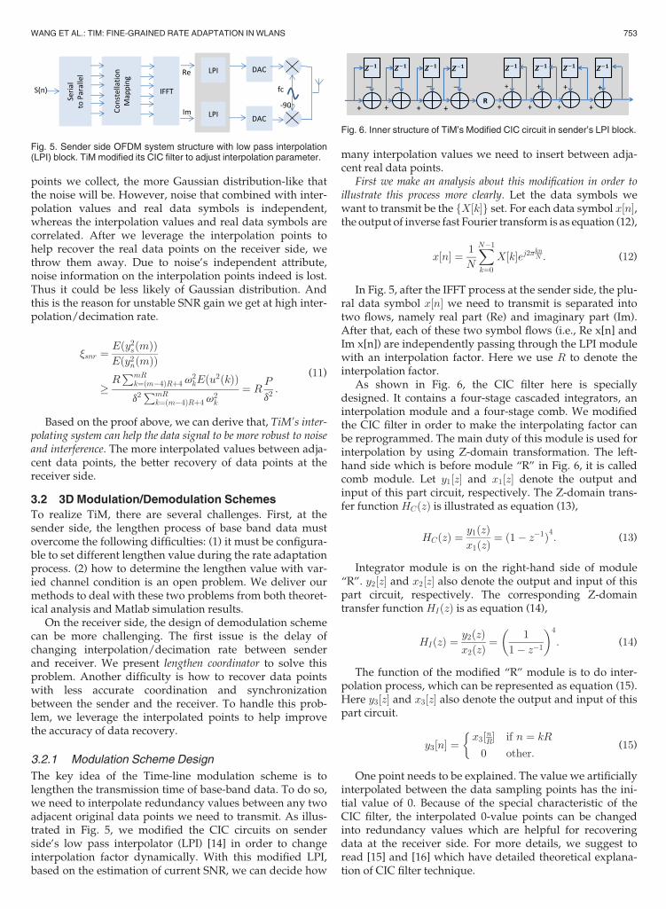
The key idea of the Time-line modulation scheme is tolengthen the transmission time of base-band data. To do so,we need to interpolate redundancy values between any twoadjacent original data points we need to transmit. As illus-trated in Fig. 5, we modified the CIC circuits on senderside’s low pass interpolator (LPI) [14] in order to changeinterpolation factor dynamically. With this modified LPI,based on the estimation of current SNR, we can decide how

many interpolation values we need to insert between adja-cent real data points.

First we make an analysis about this modification in order toillustrate this process more clearly. Let the data symbols wewant to transmit be the fX½k�g set. For each data symbol x½n�,the output of inverse fast Fourier transform is as equation (12),

x½n� ¼ 1

N

XN�1

k¼0

X½k�ej2pknN : (12)

In Fig. 5, after the IFFT process at the sender side, the plu-ral data symbol x½n� we need to transmit is separated intotwo flows, namely real part (Re) and imaginary part (Im).After that, each of these two symbol flows (i.e., Re x[n] andIm x[n]) are independently passing through the LPI modulewith an interpolation factor. Here we use R to denote theinterpolation factor.

As shown in Fig. 6, the CIC filter here is speciallydesigned. It contains a four-stage cascaded integrators, aninterpolation module and a four-stage comb. We modifiedthe CIC filter in order to make the interpolating factor canbe reprogrammed. The main duty of this module is used forinterpolation by using Z-domain transformation. The left-hand side which is before module “R” in Fig. 6, it is calledcomb module. Let y1½z� and x1½z� denote the output andinput of this part circuit, respectively. The Z-domain trans-fer functionHCðzÞ is illustrated as equation (13),

HCðzÞ ¼ y1ðzÞx1ðzÞ ¼ ð1� z�1Þ4: (13)

Integrator module is on the right-hand side of module“R”. y2½z� and x2½z� also denote the output and input of thispart circuit, respectively. The corresponding Z-domaintransfer functionHIðzÞ is as equation (14),

HIðzÞ ¼ y2ðzÞx2ðzÞ ¼

1

1� z�1

� �4

: (14)

The function of the modified “R” module is to do inter-polation process, which can be represented as equation (15).Here y3½z� and x3½z� also denote the output and input of thispart circuit.

y3½n� ¼x3½nR� if n ¼ kR

0 other:

�(15)

One point needs to be explained. The value we artificiallyinterpolated between the data sampling points has the ini-tial value of 0. Because of the special characteristic of theCIC filter, the interpolated 0-value points can be changedinto redundancy values which are helpful for recoveringdata at the receiver side. For more details, we suggest toread [15] and [16] which have detailed theoretical explana-tion of CIC filter technique.

Fig. 5. Sender side OFDM system structure with low pass interpolation(LPI) block. TiM modified its CIC filter to adjust interpolation parameter.

Fig. 6. Inner structure of TiM’s Modified CIC circuit in sender’s LPI block.


Based on these basic equations, We can derive the wholecircuit’s Z-domain transfer function as equation (16),

HðzÞ ¼ HcðzRÞ �HIðzÞ

¼ ð1� z�RÞ4 � 1

1� z�1

� �4

¼ 1� z�R

1� z�1

� �4

:

(16)

According to this Z-transfer function in equation (16), wetransfer it into time-domain and get the input x½n� and out-put y½n� of this whole modified LPI as equation (17),

y½n� ¼ 4y½n� 1� � 6y½n� 2� þ 4y½n� 3� � y½n� 4�þ x½n� � 4x½n�R� þ 6x½n� 2R� � 4x½n� 3R�þ x½n� 4R�:

(17)

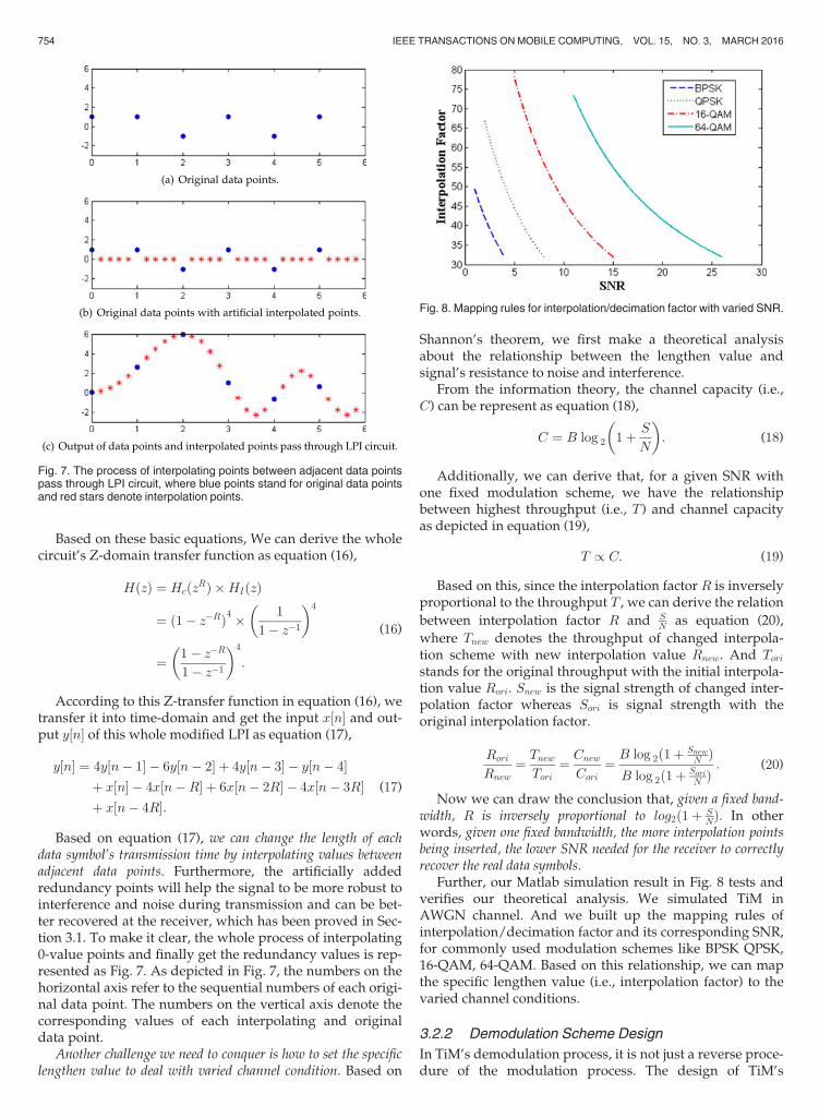
Based on equation (17), we can change the length of eachdata symbol’s transmission time by interpolating values betweenadjacent data points. Furthermore, the artificially addedredundancy points will help the signal to be more robust tointerference and noise during transmission and can be bet-ter recovered at the receiver, which has been proved in Sec-tion 3.1. To make it clear, the whole process of interpolating0-value points and finally get the redundancy values is rep-resented as Fig. 7. As depicted in Fig. 7, the numbers on thehorizontal axis refer to the sequential numbers of each origi-nal data point. The numbers on the vertical axis denote thecorresponding values of each interpolating and originaldata point.

Another challenge we need to conquer is how to set the specificlengthen value to deal with varied channel condition. Based on

Shannon’s theorem, we first make a theoretical analysisabout the relationship between the lengthen value andsignal’s resistance to noise and interference.

From the information theory, the channel capacity (i.e.,C) can be represent as equation (18),

C ¼ B log 2 1þ S

N

� �: (18)

Additionally, we can derive that, for a given SNR withone fixed modulation scheme, we have the relationshipbetween highest throughput (i.e., T ) and channel capacityas depicted in equation (19),

T / C: (19)

Based on this, since the interpolation factor R is inverselyproportional to the throughput T , we can derive the relation

between interpolation factor R and SN as equation (20),

where Tnew denotes the throughput of changed interpola-tion scheme with new interpolation value Rnew. And Tori

stands for the original throughput with the initial interpola-tion value Rori. Snew is the signal strength of changed inter-polation factor whereas Sori is signal strength with theoriginal interpolation factor.

Rori

Rnew¼ Tnew

Tori¼ Cnew

Cori¼ B log 2ð1þ Snew

N ÞB log 2ð1þ Sori

N Þ : (20)

Now we can draw the conclusion that, given a fixed band-width, R is inversely proportional to log2ð1þ S

NÞ. In otherwords, given one fixed bandwidth, the more interpolation pointsbeing inserted, the lower SNR needed for the receiver to correctlyrecover the real data symbols.

Further, our Matlab simulation result in Fig. 8 tests andverifies our theoretical analysis. We simulated TiM inAWGN channel. And we built up the mapping rules ofinterpolation/decimation factor and its corresponding SNR,for commonly used modulation schemes like BPSK QPSK,16-QAM, 64-QAM. Based on this relationship, we can mapthe specific lengthen value (i.e., interpolation factor) to thevaried channel conditions.

3.2.2 Demodulation Scheme Design

In TiM’s demodulation process, it is not just a reverse proce-dure of the modulation process. The design of TiM’s

Fig. 7. The process of interpolating points between adjacent data pointspass through LPI circuit, where blue points stand for original data pointsand red stars denote interpolation points.

Fig. 8. Mapping rules for interpolation/decimation factor with varied SNR.


demodulation scheme seems to be more challenging. Andthere are mainly two following difficulties.

First, when changing the interpolation rate, the coordi-nation between transceivers is a hard problem. How tomanage this procedure in order to minimize the overheadof rate changing delay? The module “lengthen coordinator”we proposed in Section 4 can solve this problem withnegligible overhead.

Second, when SNR varies frequently, our interpolationrate changing may also be frequent. Given this, thereceiver’s sampling rate may not be perfectly synchronizedand coordinated with the sender’s. There may exists differ-ence between the original data points and receiver’s sam-pled values. Own to our interpolation points, this distortioncan be recovered by TiM’s interpolated value. This recoveryprocedure can be regarded as another aspect of enhancingsignal’s robust attribute that TiM can achieve.

4 IMPLEMENTATION

In this section, we present a detailed implementation ofTiM. We use GNU radio [17] to implement TiM’s senderand receiver on USRP2 software radio platform [8].As depicted in Fig. 3, TiM consist of three parts, namelyGrain Size Estimation, TiM modulation/demodulation andlengthen coordinator. As mentioned in previous Section 3, themain working procedure can be illustrated as follows. First,with channel variation information, by using Grain SizeEstimation, we set proper fine-grain level to balance betweenthe overhead of changing rate and fine-grained modulationgain. Then, we implement TiM modulation/demodulationfor upper layer data encoding/decoding and leveragelengthen coordinator to reduce the rate changing head.

In following parts, We first deliver the implementationprocedure of the TiM’s modulation/demodulation designon the sender and the receiver. After that we discuss aboutlengthen coordinator and Grain Size Estimation design.

4.1 TiM’s Modulation/Demodulation SchemeImplementation

As described in Section 3.2, we need tomodifymodule “R” inthe CIC circuit of transceivers to enable that the interpola-tion/decimation factor can be reprogrammed. After thismodification, we artificially insert the interpolation points(with initial value of 0) before the interpolation process. Thenwe can change the interpolation factor based on the numberof interpolation points we insert between two adjacent realdata points. We let the data points and inserted interpolationpoints together pass through the CIC circuit and finally getthe combinedmodulated signal as the CIC’s output. Then wetransmits themodulated signal to the receiver.

On the receiver side, we demodulate the combined signalas an inverse process of the modulation procedure onthe sender side. After we decoded one specific data pointand its correlated interpolation values, we leverage theinterpolation values to make an estimation of this data pointto enhance the accuracy of data recovery. Since there arehuge amounts of value estimation algorithms (such as beliefpropagation in [18], confidence level in [19] and so on),here we use the K-means clustering algorithm [20] to dothis estimation.

4.2 PHY Preamble Modification

In order to coordinate the transceiver’s interpolation/deci-mation rate, we need to modify PHY preamble. In IEEE802.11 standard [9], modulation scheme information is con-tained in the RATE field of OFDM physical layer conver-gence protocol (PLCP) preamble.

The RATE field of OFDM PLCP preamble consists of4 bits, which can represent at most 16 modulation schemes.The current modulation schemes in use are BPSK QPSK16-QAMwith coding rate of 1/2 and 3/4, and 64-QAMwithcoding rate of 2/3 and 3/4. Therefore, there are 16� 8 ¼ 8empty positions can be used for representing additionalmodulation schemes provided by TiM. As for normal situa-tions, we believe that adding eight modulation schemes isfine-grained enough to get the near optimal goodput in awireless link. So here we leverage these 8 available positionsin RATE field to represents interpolation factor of eight addi-tional TiM’s modulation schemes. Furthermore, given morefine-grained scenarios, we can modify PHY preamble byadding additional bits on RATE field to represent a largernumber of more fine-grainedmodulation schemes in TiM.

4.3 Lengthen Coordinator

We now present the design of lengthen coordinator module,which is used for reducing the overhead of rate changing.Basically, there are two main changing overheads. One isthe delay in the rate (interpolation factor) changing process.Another is the delay of processing received data at thereceiver side. We first discuss these two delays respectively.Then we present lengthen coordinator’s scheduling algorithmto solve these two issues.

4.3.1 Delay in Changing Interpolation Rate

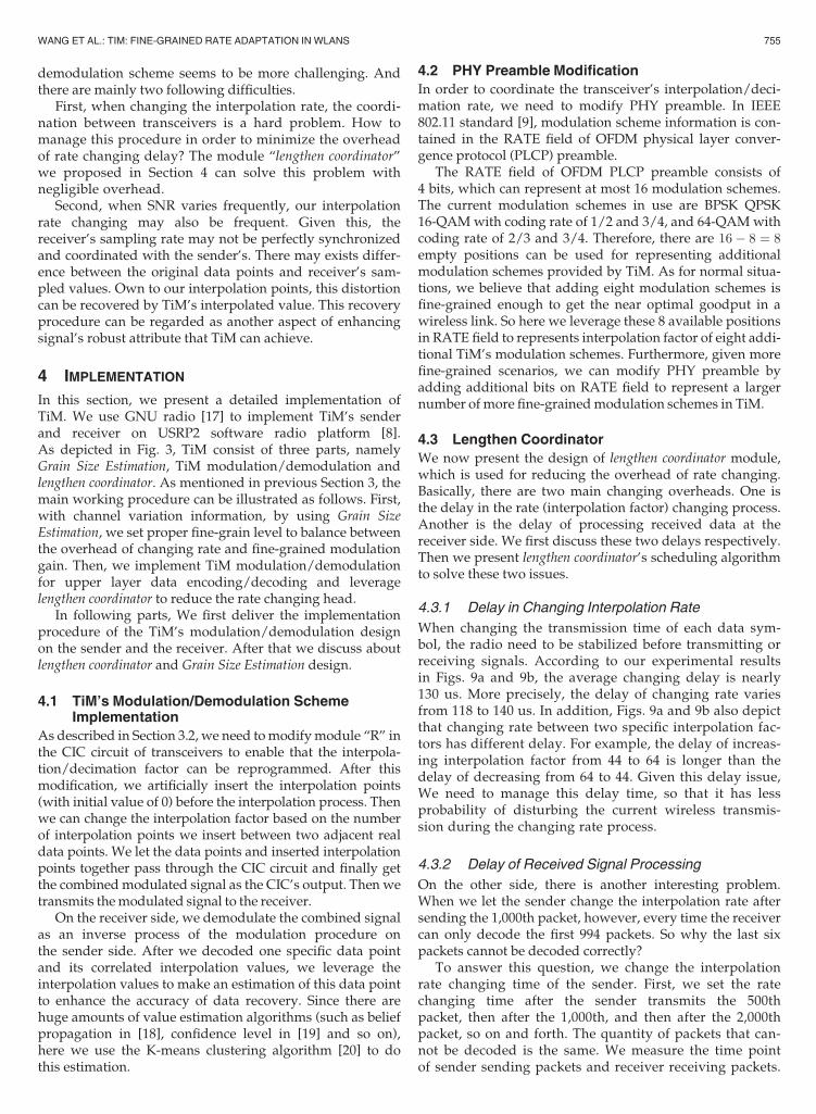
When changing the transmission time of each data sym-bol, the radio need to be stabilized before transmitting orreceiving signals. According to our experimental resultsin Figs. 9a and 9b, the average changing delay is nearly130 us. More precisely, the delay of changing rate variesfrom 118 to 140 us. In addition, Figs. 9a and 9b also depictthat changing rate between two specific interpolation fac-tors has different delay. For example, the delay of increas-ing interpolation factor from 44 to 64 is longer than thedelay of decreasing from 64 to 44. Given this delay issue,We need to manage this delay time, so that it has lessprobability of disturbing the current wireless transmis-sion during the changing rate process.

4.3.2 Delay of Received Signal Processing

On the other side, there is another interesting problem.When we let the sender change the interpolation rate aftersending the 1,000th packet, however, every time the receivercan only decode the first 994 packets. So why the last sixpackets cannot be decoded correctly?

To answer this question, we change the interpolationrate changing time of the sender. First, we set the ratechanging time after the sender transmits the 500thpacket, then after the 1,000th, and then after the 2,000thpacket, so on and forth. The quantity of packets that can-not be decoded is the same. We measure the time pointof sender sending packets and receiver receiving packets.


The data in Table 3 shows the time of emitting andreceiving packets where sender changes rate on the501th packet.

In Table 3, there is a time gap between the sender send-ing one packet and the receiver receiving that specificpacket. This is because processing delay on both sender andreceiver (e.g., packet 494, the delay between sender andreceiver is 28:43� 28:35 ¼ 0:08 ms). And this is the key rea-son why receiver cannot decode the last six packets withunchanged interpolation rate.

As in Table 3, when the receiver finish processing the494th packet, it is the same time that the sender sendsthe 501th packet. It means that the receiver’s buffer hasalready received the first 500 packets but not finishedprocessing them. And at the same time, it receives the501th packet. Since interpolation rate is not the same asthe first 500 packets, the receiver cannot decode the 501thpacket. Because of rate changing, receiver stops process-ing and empties the buffer that stores unprocessed pack-ets (i.e., 495-500). After that, the receiver received the502th packet and decoded it as normal.

4.3.3 Lengthen Coordinator Scheme Design

With the two main delays we discussed above, how toreduce the overhead is a big challenge. lengthen coordinator isa tricky scheme. Instead of directly avoiding these over-heads, it leverage these two delays to cancel with each other.

To illustrate this, we also use Table 3 as reference.After the sender emitted the 500th packet with originalinterpolation rate, it finished its rate changing process inaround 130 us. At this time, the receiver finished process-ing the 494th packet. Because the delay between senderand receiver is caused by both sides, it needs nearly halfof the total delay time (i.e., 0:08=2 ¼ 0:04 ms) for thereceiver to process one packet. Thus the receiver needs0:04 ms� 6 ¼ 240 us to finish processing the last six pack-ets in its buffer. Given this, the sender prepares the 501thpacket and doesn’t send it, this period costs 40us. At this

time the receiver has processed packet 495. The senderwaits for another 0:04 ms� 5 ¼ 200 us which is the timefor the receiver to finish processing from the 496th packetto the 500th packet. After this, the sender begins to sendthe 501th packet with changed rate. The receiver receivedthis packet and began to coordinate with the sender’s cur-rent interpolation rate. So there is only one packet (i.e.,the 501th packet) loss rather than seven (i.e., the 495th-500th packets with original rate and the 501th packetwith changed rate) loss. Additionally, at the receiver side,there is no noticeable delay because the receiver receivedthe following packet (i.e., the 501th packet) right after itprocessed the packets (i.e., the 495th-500th packet) inits buffer. In receiver’s view, it is as if the transmissionhas no delay since it always has packets received need tobe processed.

By leveraging processing delay and rate changing delayto cancel each other, we successfully reduce the overhead ofimplementing TiM into real-world systems.

4.4 Grain Size Estimation

Only based on the basic model of TiM, it cannot be imple-mented into real-world wireless networks. Before imple-menting TiM, we should first define how dense the fine-grained level we set. Grain Size Estimation can achieve thisby measuring channel variation range and frequency.

Before implementing TiM, we first make a training pro-cess of channel condition estimation. Based on the channelvariation information we collect, we analysis its variationrange and frequency. The basic principle is that the largervariation range and the higher variation frequency, we setless fine-grained levels (and vice versa) to meet with thetrade-off between rate changing overhead and fine-grainedthroughput gains. Additionally, after implementing TiM,we can further adapt fine-grained level dynamically if thechannel condition changes dramatically.

5 EVALUATION

We evaluate TiM’s performance in this section. Here wemainly focus on channel utilization, lengthen coordinatoreffect, fine-grain level effect, the transceivers’ movingeffect and energy consumption of TiM. The experimental

TABLE 3Packet Transmission Delay between Transmitter

and Receiver

Packet number Sender transmittedtime (ms)

Receiver receivedtime (ms)

491 26.52 26.6492 27.11 27.2493 27.73 27.81494 28.35 28.43495 29.09 N/A496 29.64 N/A497 30.18 N/A498 30.76 N/A499 31.37 N/A500 32.03 N/A501 32.61 N/A502 33.18 33.26

Fig. 9. Time delay in changing interpolation rate.


results demonstrate that TiM can achieve up to 200 per-cent channel utilization efficiency. Furthermore, withoutlengthen coordinator the overall goodput will decrease.Additionally, Gain Size Estimation have a significantimpact on the performance of TiM.

5.1 Channel Utilization

In this part, we evaluate TiM’s performance mainly fromthree aspects, namely the channel utilization, bit errorrate and how the nearly linear rate changing that TiM canachieve.

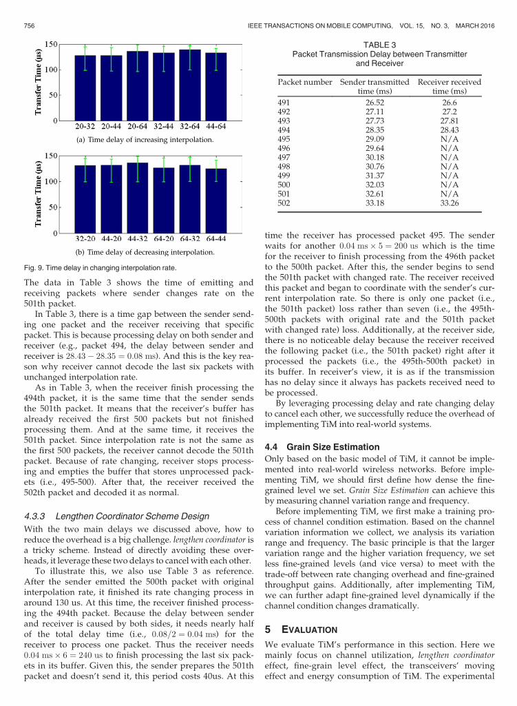
First, we compare the goodput (not throughput) of TiMwith conventional 2D modulation in three different scenar-ios, namely Low SNR (ranging from 0-10 dB), Medium SNR(10-20 dB), High SNR (20-30 dB). Note that each 2D scheme(e.g., BPSK) may have different coding rates (e.g., 1/2 3/4),here we pick up the coding rate that can achieve the highestgoodput as the coding rate for this specific 2D scheme.And we use the highest goodput to represent each scheme’sperformance. In addition, the performance of all the 2Dschemes in Figs. 10, 11, 14 and 15 follows the same rules.

As shown in Fig. 10, in low and medium SNR, TiM out-performs 2D schemes to nearly 60 percent on average.In high SNR, TiM can achieve up to 200 percent goodputcompared with 2D schemes.

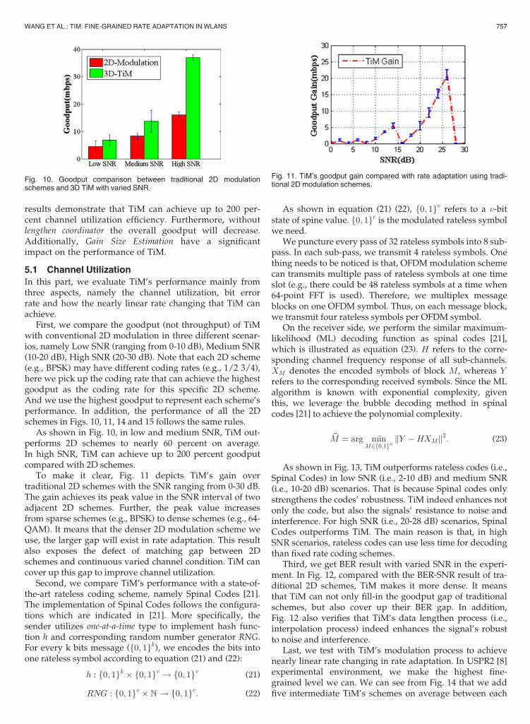
To make it clear, Fig. 11 depicts TiM’s gain overtraditional 2D schemes with the SNR ranging from 0-30 dB.The gain achieves its peak value in the SNR interval of twoadjacent 2D schemes. Further, the peak value increasesfrom sparse schemes (e.g., BPSK) to dense schemes (e.g., 64-QAM). It means that the denser 2D modulation scheme weuse, the larger gap will exist in rate adaptation. This resultalso exposes the defect of matching gap between 2Dschemes and continuous varied channel condition. TiM cancover up this gap to improve channel utilization.

Second, we compare TiM’s performance with a state-of-the-art rateless coding scheme, namely Spinal Codes [21].The implementation of Spinal Codes follows the configura-tions which are indicated in [21]. More specifically, thesender utilizes one-at-a-time type to implement hash func-tion h and corresponding random number generator RNG.For every k bits message (f0; 1gk), we encodes the bits intoone rateless symbol according to equation (21) and (22):

h : f0; 1gk � f0; 1gv ! f0; 1gv (21)

RNG : f0; 1gv �N ! f0; 1gc: (22)

As shown in equation (21) (22), f0; 1gv refers to a v-bitstate of spine value. f0; 1gc is the modulated rateless symbolwe need.

We puncture every pass of 32 rateless symbols into 8 sub-pass. In each sub-pass, we transmit 4 rateless symbols. Onething needs to be noticed is that, OFDMmodulation schemecan transmits multiple pass of rateless symbols at one timeslot (e.g., there could be 48 rateless symbols at a time when64-point FFT is used). Therefore, we multiplex messageblocks on one OFDM symbol. Thus, on each message block,we transmit four rateless symbols per OFDM symbol.

On the receiver side, we perform the similar maximum-likelihood (ML) decoding function as spinal codes [21],which is illustrated as equation (23). H refers to the corre-sponding channel frequency response of all sub-channels.XM denotes the encoded symbols of block M, whereas Yrefers to the corresponding received symbols. Since the MLalgorithm is known with exponential complexity, giventhis, we leverage the bubble decoding method in spinalcodes [21] to achieve the polynomial complexity.

bM ¼ arg minM2f0;1gn

kY �HXMk2: (23)

As shown in Fig. 13, TiM outperforms rateless codes (i.e.,Spinal Codes) in low SNR (i.e., 2-10 dB) and medium SNR(i.e., 10-20 dB) scenarios. That is because Spinal codes onlystrengthens the codes’ robustness. TiM indeed enhances notonly the code, but also the signals’ resistance to noise andinterference. For high SNR (i.e., 20-28 dB) scenarios, SpinalCodes outperforms TiM. The main reason is that, in highSNR scenarios, rateless codes can use less time for decodingthan fixed rate coding schemes.

Third, we get BER result with varied SNR in the experi-ment. In Fig. 12, compared with the BER-SNR result of tra-ditional 2D schemes, TiM makes it more dense. It meansthat TiM can not only fill-in the goodput gap of traditionalschemes, but also cover up their BER gap. In addition,Fig. 12 also verifies that TiM’s data lengthen process (i.e.,interpolation process) indeed enhances the signal’s robustto noise and interference.

Last, we test with TiM’s modulation process to achievenearly linear rate changing in rate adaptation. In USPR2 [8]experimental environment, we make the highest fine-grained level we can. We can see from Fig. 14 that we addfive intermediate TiM’s schemes on average between each

Fig. 10. Goodput comparison between traditional 2D modulationschemes and 3D TiM with varied SNR.

Fig. 11. TiM’s goodput gain compared with rate adaptation using tradi-tional 2D modulation schemes.


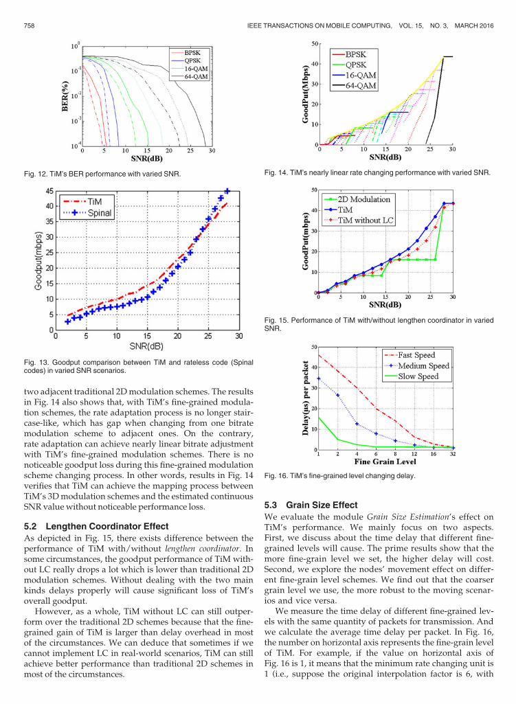
two adjacent traditional 2Dmodulation schemes. The resultsin Fig. 14 also shows that, with TiM’s fine-grained modula-tion schemes, the rate adaptation process is no longer stair-case-like, which has gap when changing from one bitratemodulation scheme to adjacent ones. On the contrary,rate adaptation can achieve nearly linear bitrate adjustmentwith TiM’s fine-grained modulation schemes. There is nonoticeable goodput loss during this fine-grained modulationscheme changing process. In other words, results in Fig. 14verifies that TiM can achieve the mapping process betweenTiM’s 3Dmodulation schemes and the estimated continuousSNR value without noticeable performance loss.

5.2 Lengthen Coordinator Effect

As depicted in Fig. 15, there exists difference between theperformance of TiM with/without lengthen coordinator. Insome circumstances, the goodput performance of TiM with-out LC really drops a lot which is lower than traditional 2Dmodulation schemes. Without dealing with the two mainkinds delays properly will cause significant loss of TiM’soverall goodput.

However, as a whole, TiM without LC can still outper-form over the traditional 2D schemes because that the fine-grained gain of TiM is larger than delay overhead in mostof the circumstances. We can deduce that sometimes if wecannot implement LC in real-world scenarios, TiM can stillachieve better performance than traditional 2D schemes inmost of the circumstances.

5.3 Grain Size Effect

We evaluate the module Grain Size Estimation’s effect onTiM’s performance. We mainly focus on two aspects.First, we discuss about the time delay that different fine-grained levels will cause. The prime results show that themore fine-grain level we set, the higher delay will cost.Second, we explore the nodes’ movement effect on differ-ent fine-grain level schemes. We find out that the coarsergrain level we use, the more robust to the moving scenar-ios and vice versa.

We measure the time delay of different fine-grained lev-els with the same quantity of packets for transmission. Andwe calculate the average time delay per packet. In Fig. 16,the number on horizontal axis represents the fine-grain levelof TiM. For example, if the value on horizontal axis ofFig. 16 is 1, it means that the minimum rate changing unit is1 (i.e., suppose the original interpolation factor is 6, with

Fig. 12. TiM’s BER performance with varied SNR.

Fig. 13. Goodput comparison between TiM and rateless code (Spinalcodes) in varied SNR scenarios.

Fig. 14. TiM’s nearly linear rate changing performance with varied SNR.

Fig. 15. Performance of TiM with/without lengthen coordinator in variedSNR.

Fig. 16. TiM’s fine-grained level changing delay.


fine-grain level of 1, the factor can be changed to 5,7 and soon). From Fig. 16, we can find out that the higher fine-grained level we set, the more delay overhead will causebecause of the frequently rate changing.

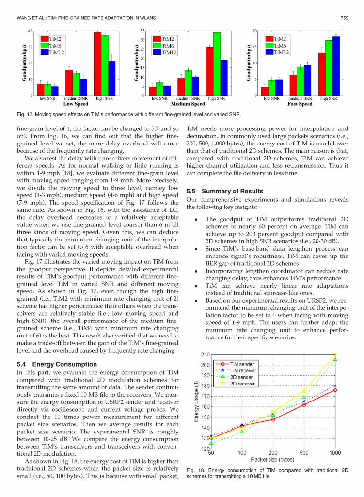
We also test the delay with transceivers movement of dif-ferent speeds. As for normal walking or little running iswithin 1-9 mph [18], we evaluate different fine-grain levelwith moving speed ranging from 1-9 mph. More precisely,we divide the moving speed to three level, namley lowspeed (1-3 mph), medium speed (4-6 mph) and high speed(7-9 mph). The speed specification of Fig. 17 follows thesame rule. As shown in Fig. 16, with the assistance of LC,the delay overhead decreases to a relatively acceptablevalue when we use fine-grained level coarser than 6 in allthree kinds of moving speed. Given this, we can deducethat typically the minimum changing unit of the interpola-tion factor can be set to 6 with acceptable overhead whenfacing with varied moving speeds.

Fig. 17 illustrates the varied moving impact on TiM fromthe goodput perspective. It depicts detailed experimentalresults of TiM’s goodput performance with different fine-grained level TiM in varied SNR and different movingspeed. As shown in Fig. 17, even though the high fine-grained (i.e., TiM2 with minimum rate changing unit of 2)scheme has higher performance than others when the trans-ceivers are relatively stable (i.e., low moving speed andhigh SNR), the overall performance of the medium fine-grained scheme (i.e., TiM6 with minimum rate changingunit of 6) is the best. This result also verified that we need tomake a trade-off between the gain of the TiM’s fine-grainedlevel and the overhead caused by frequently rate changing.

5.4 Energy Consumption

In this part, we evaluate the energy consumption of TiMcompared with traditional 2D modulation schemes fortransmitting the same amount of data. The sender continu-ously transmits a fixed 10 MB file to the receivers. We mea-sure the energy consumption of USRP2 sender and receiverdirectly via oscilloscope and current voltage probes. Weconduct the 10 times power measurement for differentpacket size scenarios. Then we average results for eachpacket size scenario. The experimental SNR is roughlybetween 10-25 dB. We compare the energy consumptionbetween TiM’s transceivers and transceivers with conven-tional 2D modulation.

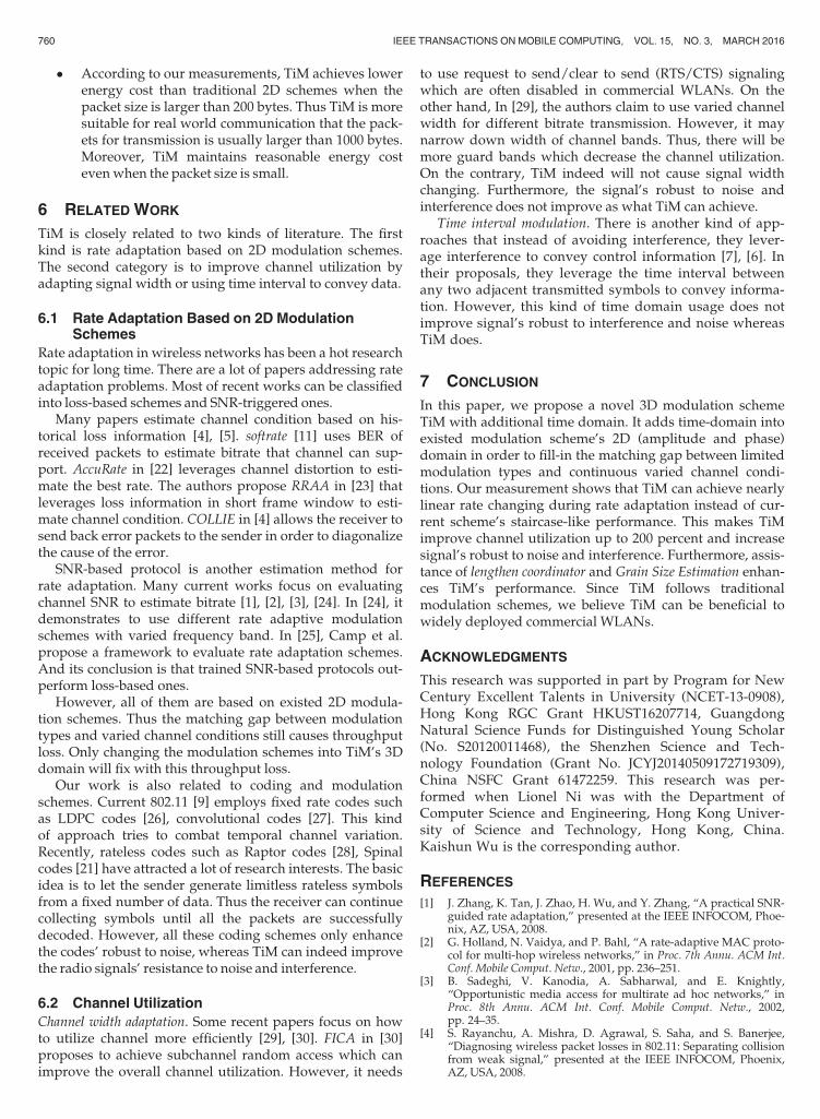
As shown in Fig. 18, the energy cost of TiM is higher thantraditional 2D schemes when the packet size is relativelysmall (i.e., 50, 100 bytes). This is because with small packet,

TiM needs more processing power for interpolation anddecimation. In commonly used large packets scenarios (i.e.,200, 500, 1,000 bytes), the energy cost of TiM is much lowerthan that of traditional 2D schemes. The main reason is that,compared with traditional 2D schemes, TiM can achievehigher channel utilization and less retransmission. Thus itcan complete the file delivery in less time.

5.5 Summary of Results

Our comprehensive experiments and simulations revealsthe following key insights:

� The goodput of TiM outperforms traditional 2Dschemes to nearly 60 percent on average. TiM canachieve up to 200 percent goodput compared with2D schemes in high SNR scenarios (i.e., 20-30 dB).

� Since TiM’s base-band data lengthen process canenhance signal’s robustness, TiM can cover up theBER gap of traditional 2D schemes.

� Incorporating lengthen coordinator can reduce ratechanging delay, thus enhances TiM’s performance.

� TiM can achieve nearly linear rate adaptationsinstead of traditional staircase-like ones.

� Based on our experimental results on URSP2, we rec-ommend the minimum changing unit of the interpo-lation factor to be set to 6 when facing with movingspeed of 1-9 mph. The users can further adapt theminimum rate changing unit to enhance perfor-mance for their specific scenarios.

Fig. 17. Moving speed effects on TiM’s performance with different fine-grained level and varied SNR.

Fig. 18. Energy consumption of TiM compared with traditional 2Dschemes for transmitting a 10 MB file.


� According to our measurements, TiM achieves lowerenergy cost than traditional 2D schemes when thepacket size is larger than 200 bytes. Thus TiM is moresuitable for real world communication that the pack-ets for transmission is usually larger than 1000 bytes.Moreover, TiM maintains reasonable energy costevenwhen the packet size is small.

6 RELATED WORK

TiM is closely related to two kinds of literature. The firstkind is rate adaptation based on 2D modulation schemes.The second category is to improve channel utilization byadapting signal width or using time interval to convey data.

6.1 Rate Adaptation Based on 2D ModulationSchemes

Rate adaptation in wireless networks has been a hot researchtopic for long time. There are a lot of papers addressing rateadaptation problems. Most of recent works can be classifiedinto loss-based schemes and SNR-triggered ones.

Many papers estimate channel condition based on his-torical loss information [4], [5]. softrate [11] uses BER ofreceived packets to estimate bitrate that channel can sup-port. AccuRate in [22] leverages channel distortion to esti-mate the best rate. The authors propose RRAA in [23] thatleverages loss information in short frame window to esti-mate channel condition. COLLIE in [4] allows the receiver tosend back error packets to the sender in order to diagonalizethe cause of the error.

SNR-based protocol is another estimation method forrate adaptation. Many current works focus on evaluatingchannel SNR to estimate bitrate [1], [2], [3], [24]. In [24], itdemonstrates to use different rate adaptive modulationschemes with varied frequency band. In [25], Camp et al.propose a framework to evaluate rate adaptation schemes.And its conclusion is that trained SNR-based protocols out-perform loss-based ones.

However, all of them are based on existed 2D modula-tion schemes. Thus the matching gap between modulationtypes and varied channel conditions still causes throughputloss. Only changing the modulation schemes into TiM’s 3Ddomain will fix with this throughput loss.

Our work is also related to coding and modulationschemes. Current 802.11 [9] employs fixed rate codes suchas LDPC codes [26], convolutional codes [27]. This kindof approach tries to combat temporal channel variation.Recently, rateless codes such as Raptor codes [28], Spinalcodes [21] have attracted a lot of research interests. The basicidea is to let the sender generate limitless rateless symbolsfrom a fixed number of data. Thus the receiver can continuecollecting symbols until all the packets are successfullydecoded. However, all these coding schemes only enhancethe codes’ robust to noise, whereas TiM can indeed improvethe radio signals’ resistance to noise and interference.

6.2 Channel Utilization

Channel width adaptation. Some recent papers focus on howto utilize channel more efficiently [29], [30]. FICA in [30]proposes to achieve subchannel random access which canimprove the overall channel utilization. However, it needs

to use request to send/clear to send (RTS/CTS) signalingwhich are often disabled in commercial WLANs. On theother hand, In [29], the authors claim to use varied channelwidth for different bitrate transmission. However, it maynarrow down width of channel bands. Thus, there will bemore guard bands which decrease the channel utilization.On the contrary, TiM indeed will not cause signal widthchanging. Furthermore, the signal’s robust to noise andinterference does not improve as what TiM can achieve.

Time interval modulation. There is another kind of app-roaches that instead of avoiding interference, they lever-age interference to convey control information [7], [6]. Intheir proposals, they leverage the time interval betweenany two adjacent transmitted symbols to convey informa-tion. However, this kind of time domain usage does notimprove signal’s robust to interference and noise whereasTiM does.

7 CONCLUSION

In this paper, we propose a novel 3D modulation schemeTiM with additional time domain. It adds time-domain intoexisted modulation scheme’s 2D (amplitude and phase)domain in order to fill-in the matching gap between limitedmodulation types and continuous varied channel condi-tions. Our measurement shows that TiM can achieve nearlylinear rate changing during rate adaptation instead of cur-rent scheme’s staircase-like performance. This makes TiMimprove channel utilization up to 200 percent and increasesignal’s robust to noise and interference. Furthermore, assis-tance of lengthen coordinator and Grain Size Estimation enhan-ces TiM’s performance. Since TiM follows traditionalmodulation schemes, we believe TiM can be beneficial towidely deployed commercial WLANs.

ACKNOWLEDGMENTS

This research was supported in part by Program for NewCentury Excellent Talents in University (NCET-13-0908),Hong Kong RGC Grant HKUST16207714, GuangdongNatural Science Funds for Distinguished Young Scholar(No. S20120011468), the Shenzhen Science and Tech-nology Foundation (Grant No. JCYJ20140509172719309),China NSFC Grant 61472259. This research was per-formed when Lionel Ni was with the Department ofComputer Science and Engineering, Hong Kong Univer-sity of Science and Technology, Hong Kong, China.Kaishun Wu is the corresponding author.

REFERENCES

[1] J. Zhang, K. Tan, J. Zhao, H. Wu, and Y. Zhang, “A practical SNR-guided rate adaptation,” presented at the IEEE INFOCOM, Phoe-nix, AZ, USA, 2008.

[2] G. Holland, N. Vaidya, and P. Bahl, “A rate-adaptive MAC proto-col for multi-hop wireless networks,” in Proc. 7th Annu. ACM Int.Conf. Mobile Comput. Netw., 2001, pp. 236–251.

[3] B. Sadeghi, V. Kanodia, A. Sabharwal, and E. Knightly,“Opportunistic media access for multirate ad hoc networks,” inProc. 8th Annu. ACM Int. Conf. Mobile Comput. Netw., 2002,pp. 24–35.

[4] S. Rayanchu, A. Mishra, D. Agrawal, S. Saha, and S. Banerjee,“Diagnosing wireless packet losses in 802.11: Separating collisionfrom weak signal,” presented at the IEEE INFOCOM, Phoenix,AZ, USA, 2008.


[5] J. Kim, S. Kim, S. Choi, and D. Qiao, “Cara: Collision-aware rateadaptation for ieee 802.11 WLANs,” in Proc. IEEE INFOCOM,2006, pp. 1–11.

[6] K. Wu, H. Tan, Y. Liu, J. Zhang, Q. Zhang, and L. M. Ni, “Sidechannel: Bits over interference,” in Proc. ACM 16th Annu. Int.Conf. Mobile Comput. Netw., 2010, pp. 13–24.

[7] A. Cidon, K. Nagaraj, S. Katti, and P. Viswanath, “Flashback:Decoupled lightweight wireless control,” in Proc. ACM SIGCOMMConf. Appl., Technol., Archit., Protocols Comput. Commun., 2012,pp. 223–234.

[8] E. R. LLC, Universal Software Radio Peripheral [Online]. Available:http://www.ettus.com

[9] E. Blossom, Wireless LAN Medium Access Control (MAC) and Physi-cal Layer (PHY) Specifications, IEEE Std 802.11, 2012.

[10] K. C.-J. Lin, N. Kushman, and D. Katabi, “Ziptx: Harnessing par-tial packets in 802.11 networks,” in Proc. ACM 14th Annu. Int.Conf. Mobile Comput. Netw., 2008, pp. 351–362.

[11] M. Vutukuru, H. Balakrishnan, and K. Jamieson, “Cross-layerwireless bit rate adaptation,” in Proc. ACM SIGCOMM Conf. DataCommun., 2009, pp. 3–14.

[12] F. Lu, G. M. Voelker, and A. C. Snoeren, “Slomo: Downclockingwifi communication,” in Proc. USENIX Conf. Netw. Syst. DesignImplementation, 2013, pp. 255–258.

[13] X. Zhang and K. G. Shin, “E-mili: Energy-minimizing idle listen-ing in wireless networks,” in Proc. ACM 17th Annu. Int. Conf.Mobile Comput. Netw., 2011, pp. 205–216.

[14] M. E. Frerking, Digital Signal Processing in Communication Systems.Norwell, MA, USA: Kluwer, 1993.

[15] R. G. Lyons,Understanding Digital Signal Processing, 2nd ed. UpperSaddle River, NJ, USA: Prentice Hall PTR, 2004.

[16] J. Y. Kwentus, Z. Jiang, and A. N. Willson, “Application of filtersharpening to cascaded integrator-comb decimation filters,” IEEETrans. Signal Process., vol. 45, no. 2, pp. 457–467, Feb. 1997.

[17] E. Blossom, Gnu Software Defined Radio [Online]. Available:http://www.gnu.org/software/gnuradio

[18] S. T. Aditya and S. Katti, “Flexcast: Graceful wireless videostreaming,” in Proc. ACM 17th Annu. Int. Conf. Mobile Comput.Netw., 2011, pp. 277–288.

[19] K. Jamieson and H. Balakrishnan, “PPR: Partial packet recoveryfor wireless networks,” in Proc. ACM Conf. Appl., Technol., Archit.,Protocols Comput. Commun., 2007, pp. 409–420.

[20] J. Han and M. Kamber, Data Mining: Concepts and Techniques, 2nded. San Francisco, CA, USA: Morgan Kaufmann, 2006.

[21] J. Perry, P. A. lannucci, K. Fleming, HariBalakrishnan, andD. Shah, “Spinal codes,” in Proc. ACM Conf. Appl., Technol., Archit.,Protocols Comput. Commun., 2012, pp. 49–60.

[22] S. Sen, N. Santhapuri, R. R. Choudhury, and S. Nelakuditi,“Accurate: Constellation based rate estimation in wirelessnetworks,” in Proc. 7th USENIX Conf. Netw. Syst. Design Implemen-tation, 2010, p. 12.

[23] S. H. Wong, H. Yang, S. Lu, and V. Bharghavan, “Robust rateadaptation for 802.11 wireless networks,” in Proc. ACM 12thAnnu. Int. Conf. Mobile Comput. Netw., 2006, pp. 146–157.

[24] H. Rahul, F. Edalat, D. Katabi, and C. Sodini, “Frequency-awarerate adaptation and MAC protocols,” in Proc. ACM 15th Annu. Int.Conf. Mobile Comput. Netw., 2009, pp. 193–204.

[25] J. Camp and E. Knightly, “Modulation rate adaptation in urbanand vehicular environments: Cross-layer implementation andexperimental evaluation,” in Proc. ACM 14th Annu. Int. Conf.Mobile Comput. Netw., 2008, pp. 315–326.

[26] R. Gallager, “Low-density parity-check codes,” IEEE Trans. Inf.Theory, vol. IT-8, no. 1, pp. 21–28, Jan. 1962.

[27] A. Viterbi, “Error bounds for convolutional codes and an asymp-totically optimum decoding algorithm,” IEEE Trans. Inf. Theory,vol. 13, no. 2, pp. 260–269, Apr. 1967.

[28] A. Shokrollahi, “Raptor codes,” IEEE Trans. Inf. Theory, vol. 52,no. 6, pp. 2551–2567, Jun. 2006.

[29] R. Chandra, R. Mahajan, T. Moscibroda, R. Raghhavendra, andP. Bahl, “A case for adapting channel width in wirelessnetworks,” in Proc. ACM Conf. Appl., Technol., Archit., ProtocolsComput. Commun., 2008, pp. 135–146.

[30] K. Tan, J. Fang, Y. Zhang, S. Chen, L. Shi, J. Zhang, and Y. Zhang,“Fine-grained channel access in wireless LAN,” in Proc. ACMConf. Appl., Technol., Archit., Protocols Comput. Commun., 2010,pp. 147–158.

Guanhua Wang received the BEng degree fromSoutheast University, Nanjing, China, in 2012,and is currently a master of philosophy student incomputer science and engineering, Hong KongUniversity of Science and Technology. He willstart working toward the PhD degree at AMPLabin Computer Science Division, UC Berkeley,in Fall 2015. His main research interests includeWi-Fi radar, wireless communications, andmobilecomputing. He is a student member of the IEEE.

Shanfeng Zhang received the BEng degreefrom Shanghai Jiao Tong University, Shanghai,China, in 2012, and is currently working towardthe PhD degree in computer science and engi-neering at the Hong Kong University of Scienceand Technology. His main research interestsinclude wireless communications, mobile sens-ing, and vehicular networks.

Kaishun Wu received the PhD degree in com-puter science and engineering from Hong KongUniversity of Science and Technology (HKUST)in 2011. He is currently a distinguished professorat Shenzhen University. He received the HongKong Young Scientist Award in 2012 and theIEEE ComSoc Asia-Pacific Outstanding YoungResearcher Award in 2014. His research inter-ests include wireless communication, mobilecomputing, wireless sensor networks, and wear-able computing. He is a member of the IEEE.

Qian Zhang received the PhD degree fromWuhan University, China, in 1999. She joined theHong Kong University of Science and Technol-ogy in September 2005, where she is a full pro-fessor in the Department of Computer Scienceand Engineering. Her current research interestsinclude wireless communications, IP networking,multimedia, P2P overlay, and wireless security.She is a fellow of the IEEE.

Lionel M. Ni received the PhD degree inelectrical and computer engineering from PurdueUniversity in 1980. He is a chair professor inthe Department of Computer and InformationScience and vice rector of Academic Affairs atthe University of Macau. Previously, he was achair professor of computer science and engi-neering at the Hong Kong University of Scienceand Technology. He has chaired more than 30professional conferences and has received eightawards for authoring outstanding papers. He is a

fellow of the IEEE and Hong Kong Academy of Engineering Science.

" For more information on this or any other computing topic,please visit our Digital Library at www.computer.org/publications/dlib.


Documents

748 IEEE TRANSACTIONS ON MOBILE COMPUTING, …guanhua/paper/07084168.pdf · they leverage different time intervals between transmitted symbols to represent information. However, this