Embed Size (px)
Citation preview
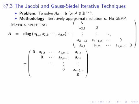
§7.3 The Jacobi and Gauss-Siedel Iterative TechniquesI Problem: To solve Ax = b for A ∈ Rn×n.I Methodology: Iteratively approximate solution x. No GEPP.
Matrix splitting
A = diag (a1,1, a2,2, · · · , an,n) +
0
a2,1 0...
.... . .
an−1,1 an−1,2 · · · 0an,1 an,2 · · · an,n−1 0
+
0 a1,2 · · · a1,n−1 a1,n
0 · · · a2,n−1 a2,n
. . ....
...0 an−1,n
0
def= D − L− U =
−
−
.
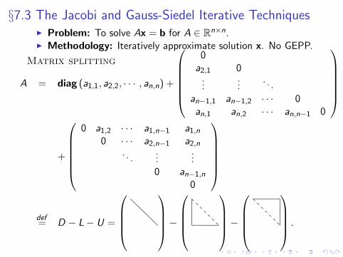
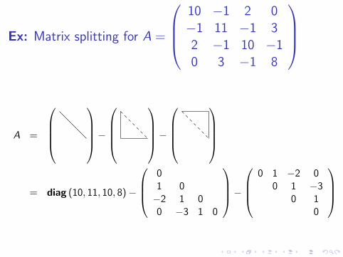
Ex: Matrix splitting for A =
10 −1 2 0−1 11 −1 32 −1 10 −10 3 −1 8
A =
−
−
= diag (10, 11, 10, 8)−
01 0−2 1 00 −3 1 0
−
0 1 −2 00 1 −3
0 10
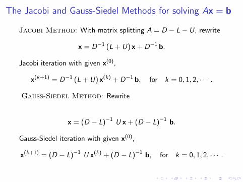
The Jacobi and Gauss-Siedel Methods for solving Ax = b
Jacobi Method: With matrix splitting A = D − L− U, rewrite
x = D−1 (L + U) x + D−1 b.
Jacobi iteration with given x(0),
x(k+1) = D−1 (L + U) x(k) + D−1 b, for k = 0, 1, 2, · · · .
Gauss-Siedel Method: Rewrite
x = (D − L)−1 U x + (D − L)−1 b.
Gauss-Siedel iteration with given x(0),
x(k+1) = (D − L)−1 U x(k) + (D − L)−1 b, for k = 0, 1, 2, · · · .
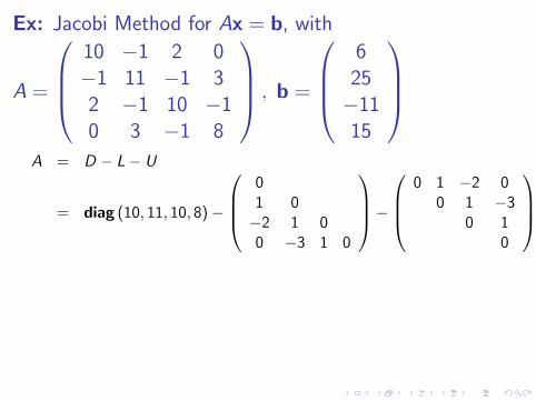
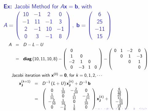
Ex: Jacobi Method for Ax = b, with
A =
10 −1 2 0−1 11 −1 32 −1 10 −10 3 −1 8
, b =
6
25−1115
A = D − L− U
= diag (10, 11, 10, 8)−
01 0−2 1 00 −3 1 0
−
0 1 −2 00 1 −3
0 10
.
Jacobi iteration with x(0) = 0, for k = 0, 1, 2, · · ·
x(k+1)J = D−1 (L + U) x
(k)J + D−1 b
=
0 1
10 − 210 0
111 0 1
11 − 311
− 210
110 0 1
100 −3
818 0
x(k)J +
6
102511−11
10158
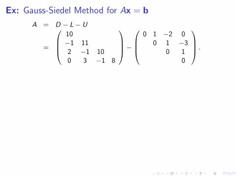
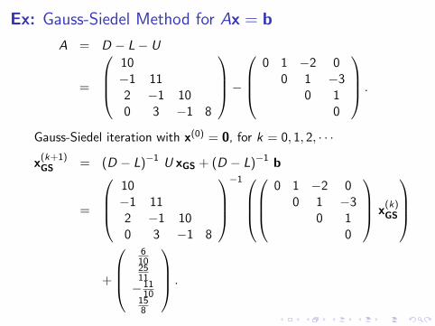
Ex: Gauss-Siedel Method for Ax = b
A = D − L− U
=
10−1 112 −1 100 3 −1 8
−
0 1 −2 00 1 −3
0 10
.
Gauss-Siedel iteration with x(0) = 0, for k = 0, 1, 2, · · ·
x(k+1)GS = (D − L)−1 U xGS + (D − L)−1 b
=
10−1 112 −1 100 3 −1 8
−1
0 1 −2 0
0 1 −30 1
0
x(k)GS
+
6
102511−11
10158
.
Ex: Gauss-Siedel Method for Ax = b
A = D − L− U
=
10−1 112 −1 100 3 −1 8
−
0 1 −2 00 1 −3
0 10
.
Gauss-Siedel iteration with x(0) = 0, for k = 0, 1, 2, · · ·
x(k+1)GS = (D − L)−1 U xGS + (D − L)−1 b
=
10−1 112 −1 100 3 −1 8
−1
0 1 −2 0
0 1 −30 1
0
x(k)GS
+
6
102511−11
10158
.
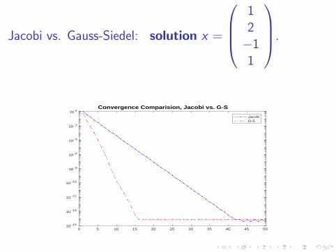
Jacobi vs. Gauss-Siedel: solution x =
12−11
.
0 5 10 15 20 25 30 35 40 45 5010 -16
10 -14
10 -12
10 -10
10 -8
10 -6
10 -4
10 -2
10 0Convergence Comparision, Jacobi vs. G-S
JacobiG-S
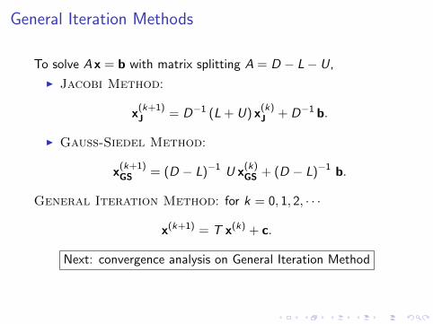
General Iteration Methods
To solve A x = b with matrix splitting A = D − L− U,
I Jacobi Method:
x(k+1)J = D−1 (L + U) x
(k)J + D−1 b.
I Gauss-Siedel Method:
x(k+1)GS = (D − L)−1 U x
(k)GS + (D − L)−1 b.
General Iteration Method: for k = 0, 1, 2, · · ·
x(k+1) = T x(k) + c.
Next: convergence analysis on General Iteration Method
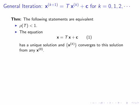
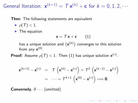
General Iteration: x(k+1) = T x(k) + c for k = 0, 1, 2, · · ·
Thm: The following statements are equivalent
I ρ(T ) < 1.
I The equationx = T x + c (1)
has a unique solution and {x(k)} converges to this solutionfrom any x(0).
Proof: Assume ρ(T ) < 1. Then (1) has unique solution x(∗).
x(k+1) − x(∗) = T(x(k) − x(∗)
)= T 2
(x(k−1) − x(∗)
)= · · · = T k+1
(x(0) − x(∗)
)=⇒ 0.
Conversely, if · · · (omitted)
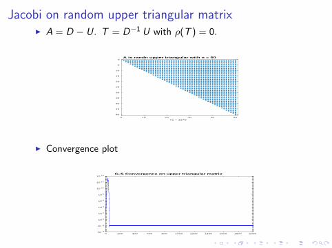
Jacobi on random upper triangular matrixI A = D − U. T = D−1 U with ρ(T ) = 0.
0 10 20 30 40 50
nz = 1275
0
5
10
15
20
25
30
35
40
45
50
A is randn upper triangular with n = 50
I Convergence plot
0 200 400 600 800 1000 1200 1400 1600 1800 200010 -4
10 -2
10 0
10 2
10 4
10 6
10 8
10 10
10 12
10 14G-S Convergence on upper triangular matrix
§7.4 Relaxation Techniques for Solving Linear SystemsTo solve A x = b with matrix splitting A = D − L− U, rewrite
D x = D x,
ω L x = ω (D − U) x− ω b, for any ω.
Taking difference of two equations,
(D − ω L) x = ((1− ω)D + ωU) x + ω b.
Successive Over-Relaxation (SOR), for k = 0, 1, 2, · · ·
x(k+1)SOR = (D − ω L)−1 ((1− ω)D + ωU) x
(k)SOR + ω (D − ω L)−1 b
def= TSOR x
(k)SOR + cSOR.
converges if ρ (TSOR) < 1.
Good choice of ω is tricky, but critical for accelerated convergence
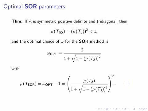
Optimal SOR parameters
Thm: If A is symmetric positive definite and tridiagonal, then
ρ (TGS) = (ρ (TJ))2 < 1,
and the optimal choice of ω for the SOR method is
ωOPT =2
1 +√
1− (ρ (TJ))2
with
ρ (TSOR) = ωOPT − 1 =
ρ (TJ)
1 +√
1− (ρ (TJ))2
2
.
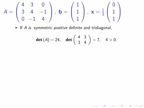
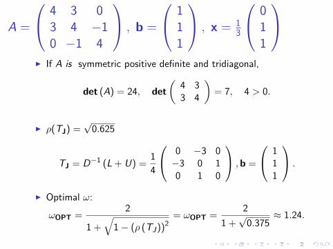
A =
4 3 03 4 −10 −1 4
, b =
111
, x = 13
011
I If A is symmetric positive definite and tridiagonal,
det (A) = 24, det
(4 33 4
)= 7, 4 > 0.
I ρ(TJ) =√
0.625
TJ = D−1 (L + U) =1
4
0 −3 0−3 0 10 1 0
,b =
111
.
I Optimal ω:
ωOPT =2
1 +√
1− (ρ (TJ))2= ωOPT =
2
1 +√
0.375≈ 1.24.
A =
4 3 03 4 −10 −1 4
, b =
111
, x = 13
011
I If A is symmetric positive definite and tridiagonal,
det (A) = 24, det
(4 33 4
)= 7, 4 > 0.
I ρ(TJ) =√
0.625
TJ = D−1 (L + U) =1
4
0 −3 0−3 0 10 1 0
,b =
111
.
I Optimal ω:
ωOPT =2
1 +√
1− (ρ (TJ))2= ωOPT =
2
1 +√
0.375≈ 1.24.
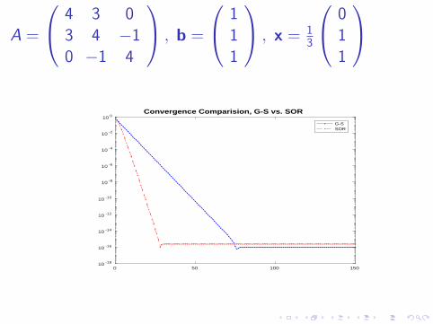
A =
4 3 03 4 −10 −1 4
, b =
111
, x = 13
011
I
0 50 100 15010 -18
10 -16
10 -14
10 -12
10 -10
10 -8
10 -6
10 -4
10 -2
10 0Convergence Comparision, G-S vs. SOR
G-SSOR
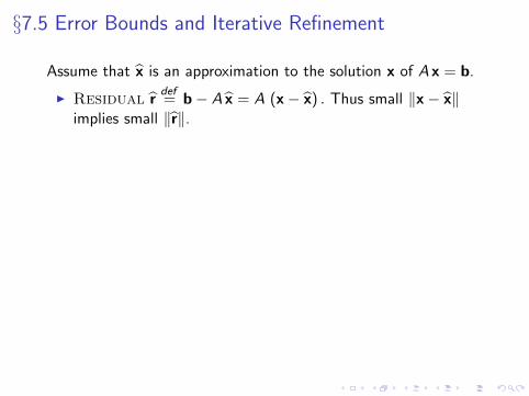
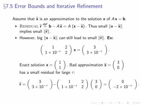
§7.5 Error Bounds and Iterative Refinement
Assume that x̂ is an approximation to the solution x of A x = b.
I Residual r̂def= b− A x̂ = A (x− x̂) . Thus small ‖x− x̂‖
implies small ‖̂r‖.
I However, big ‖x− x̂‖ can still lead to small ‖̂r‖. Ex:(1 2
1 + 10−τ 2
)x =
(3
3 + 10−τ
).
Exact solution x =
(11
). Bad approximation x̂ =
(30
)has a small residual for large τ :
r̂ =
(3
3 + 10−τ
)−(
1 21 + 10−τ 2
) (30
)=
(0
−2× 10−τ
).
§7.5 Error Bounds and Iterative Refinement
Assume that x̂ is an approximation to the solution x of A x = b.
I Residual r̂def= b− A x̂ = A (x− x̂) . Thus small ‖x− x̂‖
implies small ‖̂r‖.I However, big ‖x− x̂‖ can still lead to small ‖̂r‖. Ex:(
1 21 + 10−τ 2
)x =
(3
3 + 10−τ
).
Exact solution x =
(11
). Bad approximation x̂ =
(30
)has a small residual for large τ :
r̂ =
(3
3 + 10−τ
)−(
1 21 + 10−τ 2
) (30
)=
(0
−2× 10−τ
).
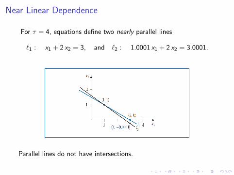
Near Linear Dependence
For τ = 4, equations define two nearly parallel lines
`1 : x1 + 2 x2 = 3, and `2 : 1.0001 x1 + 2 x2 = 3.0001.
Parallel lines do not have intersections.
Let A x = b with non-singular A and non-zero b
T¯
hm: Assume x̂ is an approximate solution with r̂ = b−A x̂. Thenfor any natural norm,
‖x̂− x‖ ≤∥∥A−1
∥∥ ‖̂r‖ ,‖x̂− x‖‖x‖
≤ κ (A)‖̂r‖‖b‖
,
where κ (A)def= ‖A‖
∥∥A−1∥∥ is the condition number of A
I A is well-conditioned if κ (A) = O(1):
small residual implies small solution error.
I A is ill-conditioned if κ (A)� 1:
small residual may still allow large solution error.
Ex: Condition Number for A =
(1 2
1 + 10−τ 2
)
Solution: For τ > 0, ‖A‖∞ = 3 + 10−τ . Since
A−1 = −10τ
2
(2 −2
− (1 + 10−τ ) 1
),
we have∥∥A−1
∥∥∞ = 2× 10τ . Thus
κ (A) = ‖A‖∞∥∥A−1
∥∥∞ = 6× 10τ + 2.
κ (A) grows exponentially in τ . A is ill-conditioned for large τ .
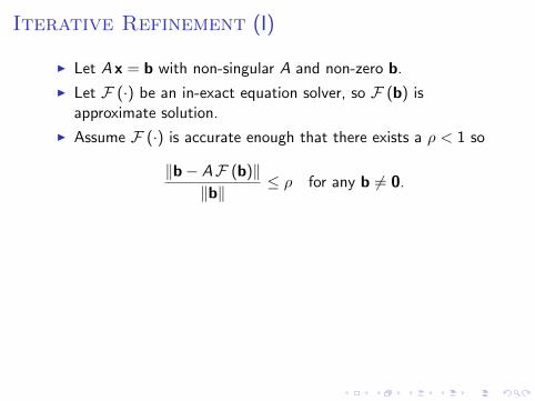
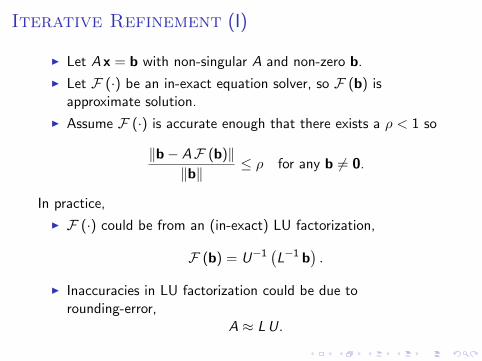
Iterative Refinement (I)
I Let A x = b with non-singular A and non-zero b.
I Let F (·) be an in-exact equation solver, so F (b) isapproximate solution.
I Assume F (·) is accurate enough that there exists a ρ < 1 so
‖b− AF (b)‖‖b‖
≤ ρ for any b 6= 0.
In practice,
I F (·) could be from an (in-exact) LU factorization,
F (b) = U−1(L−1 b
).
I Inaccuracies in LU factorization could be due torounding-error,
A ≈ LU.
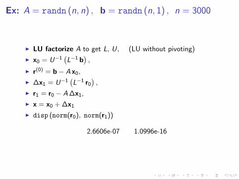
Ex: A = randn (n, n) , b = randn (n, 1) , n = 3000
I LU factorize A to get L, U, (LU without pivoting)
I x0 = U−1(L−1 b
),
I r(0) = b− A x0,
I ∆x1 = U−1(L−1 r0
),
I r1 = r0 − A∆x1,
I x = x0 + ∆x1
I disp (norm(r0), norm(r1))
2.6606e-07 1.0996e-16
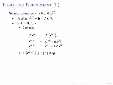
Iterative Refinement (II)
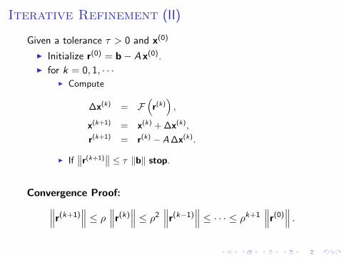
Given a tolerance τ > 0 and x(0)
I Initialize r(0) = b− A x(0).I for k = 0, 1, · · ·
I Compute
∆x(k) = F(r(k)),
x(k+1) = x(k) + ∆x(k),
r(k+1) = r(k) − A∆x(k).
I If∥∥r(k+1)
∥∥ ≤ τ ‖b‖ stop.
Convergence Proof:∥∥∥r(k+1)∥∥∥ ≤ ρ ∥∥∥r(k)
∥∥∥ ≤ ρ2∥∥∥r(k−1)
∥∥∥ ≤ · · · ≤ ρk+1∥∥∥r(0)
∥∥∥ .
Iterative Refinement (II)
Given a tolerance τ > 0 and x(0)
I Initialize r(0) = b− A x(0).I for k = 0, 1, · · ·
I Compute
∆x(k) = F(r(k)),
x(k+1) = x(k) + ∆x(k),
r(k+1) = r(k) − A∆x(k).
I If∥∥r(k+1)
∥∥ ≤ τ ‖b‖ stop.
Convergence Proof:∥∥∥r(k+1)∥∥∥ ≤ ρ ∥∥∥r(k)
∥∥∥ ≤ ρ2∥∥∥r(k−1)
∥∥∥ ≤ · · · ≤ ρk+1∥∥∥r(0)
∥∥∥ .
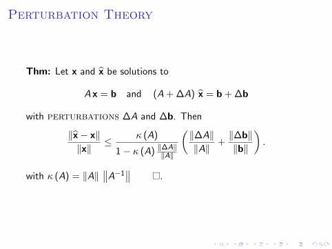
Perturbation Theory
Thm: Let x and x̂ be solutions to
A x = b and (A + ∆A) x̂ = b + ∆b
with perturbations ∆A and ∆b. Then
‖x̂− x‖‖x‖
≤ κ (A)
1− κ (A) ‖∆A‖‖A‖
(‖∆A‖‖A‖
+‖∆b‖‖b‖
).
with κ (A) = ‖A‖∥∥A−1
∥∥ .
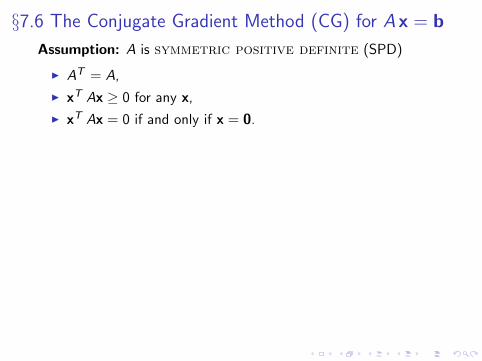
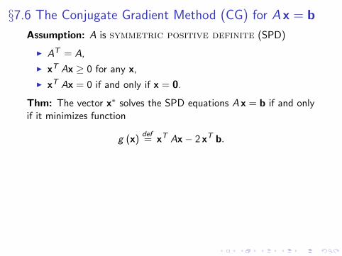
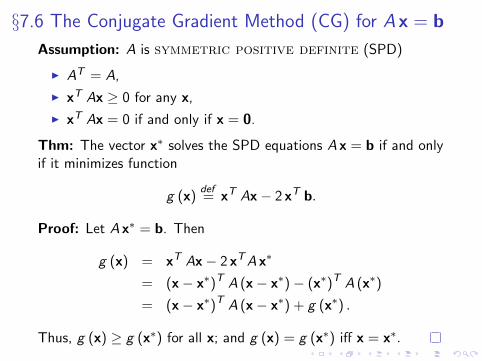
§7.6 The Conjugate Gradient Method (CG) for A x = b
Assumption: A is symmetric positive definite (SPD)
I AT = A,
I xT Ax ≥ 0 for any x,
I xT Ax = 0 if and only if x = 0.
Thm: The vector x∗ solves the SPD equations A x = b if and onlyif it minimizes function
g (x)def= xT Ax− 2 xT b.
Proof: Let A x∗ = b. Then
g (x) = xT Ax− 2 xTA x∗
= (x− x∗)T A (x− x∗)− (x∗)T A (x∗)
= (x− x∗)T A (x− x∗) + g (x∗) .
Thus, g (x) ≥ g (x∗) for all x; and g (x) = g (x∗) iff x = x∗.
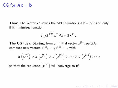
CG for A x = b
Thm: The vector x∗ solves the SPD equations A x = b if and onlyif it minimizes function
g (x)def= xT Ax− 2 xT b.
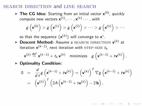
The CG Idea: Starting from an initial vector x(0), quicklycompute new vectors x(1), · · · , x(k) · · · , with
g(x(0))> g
(x(1))> g
(x(2))> · · · > g
(x(k)
)> · · ·
so that the sequence {x(k)} will converge to x∗.
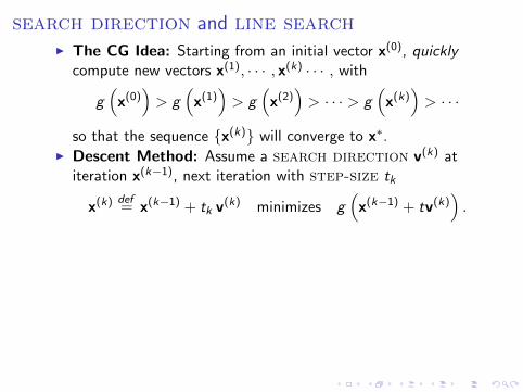
search direction and line searchI The CG Idea: Starting from an initial vector x(0), quickly
compute new vectors x(1), · · · , x(k) · · · , with
g(x(0))> g
(x(1))> g
(x(2))> · · · > g
(x(k)
)> · · ·
so that the sequence {x(k)} will converge to x∗.
I Descent Method: Assume a search direction v(k) atiteration x(k−1), next iteration with step-size tk
x(k) def= x(k−1) + tk v
(k) minimizes g(x(k−1) + tv(k)
).
I Optimality Condition:
0 =d
d tg(x(k−1) + tv(k)
)=(v(k)
)T∇g
(x(k−1) + tv(k)
)=
(v(k)
)T (2A(x(k−1) + tv(k)
)− 2b
),
tk =
(v(k)
)T (r(k−1)
)(v(k)
)T (A v(k)
) , r(k−1) def= b− A x(k−1) (residual).
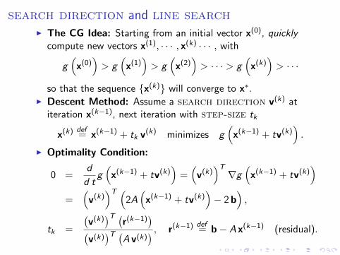
search direction and line searchI The CG Idea: Starting from an initial vector x(0), quickly
compute new vectors x(1), · · · , x(k) · · · , with
g(x(0))> g
(x(1))> g
(x(2))> · · · > g
(x(k)
)> · · ·
so that the sequence {x(k)} will converge to x∗.I Descent Method: Assume a search direction v(k) at
iteration x(k−1), next iteration with step-size tk
x(k) def= x(k−1) + tk v
(k) minimizes g(x(k−1) + tv(k)
).
I Optimality Condition:
0 =d
d tg(x(k−1) + tv(k)
)=(v(k)
)T∇g
(x(k−1) + tv(k)
)=
(v(k)
)T (2A(x(k−1) + tv(k)
)− 2b
),
tk =
(v(k)
)T (r(k−1)
)(v(k)
)T (A v(k)
) , r(k−1) def= b− A x(k−1) (residual).
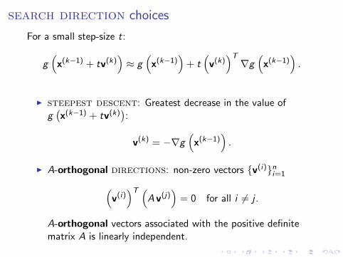
search direction choices
For a small step-size t:
g(x(k−1) + tv(k)
)≈ g
(x(k−1)
)+ t
(v(k)
)T∇g
(x(k−1)
).
I steepest descent: Greatest decrease in the value ofg(x(k−1) + tv(k)
):
v(k) = −∇g(x(k−1)
).
I A-orthogonal directions: non-zero vectors {v(i)}ni=1(v(i))T (
A v(j))
= 0 for all i 6= j .
A-orthogonal vectors associated with the positive definitematrix A is linearly independent.

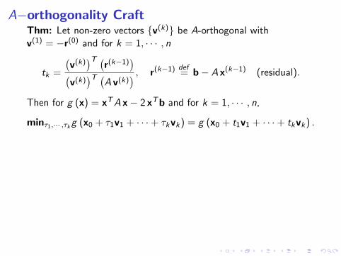
A−orthogonality Craft
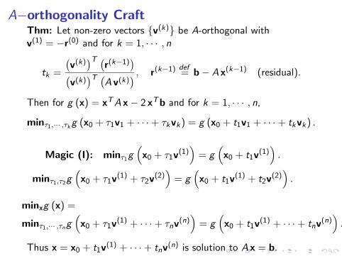
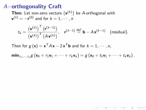
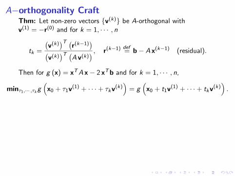
Thm: Let non-zero vectors {v(k)} be A-orthogonal withv(1) = −r(0) and for k = 1, · · · , n
tk =
(v(k)
)T (r(k−1)
)(v(k)
)T (A v(k)
) , r(k−1) def= b− A x(k−1) (residual).
Then for g (x) = xTA x− 2 xTb and for k = 1, · · · , n,
minτ1,··· ,τkg (x0 + τ1v1 + · · ·+ τkvk) = g (x0 + t1v1 + · · ·+ tkvk) .
Magic (I): minτ1g(x0 + τ1v
(1))
= g(x0 + t1v
(1)).
minτ1,τ2g(x0 + τ1v
(1) + τ2v(2))
= g(x0 + t1v
(1) + t2v(2)).
minxg (x) =
minτ1,··· ,τng(x0 + τ1v
(1) + · · ·+ τnv(n))
= g(x0 + t1v
(1) + · · ·+ tnv(n)).
Thus x = x0 + t1v(1) + · · ·+ tnv(n) is solution to A x = b.
A−orthogonality CraftThm: Let non-zero vectors {v(k)} be A-orthogonal withv(1) = −r(0) and for k = 1, · · · , n
tk =
(v(k)
)T (r(k−1)
)(v(k)
)T (A v(k)
) , r(k−1) def= b− A x(k−1) (residual).
Then for g (x) = xTA x− 2 xTb and for k = 1, · · · , n,
minτ1,··· ,τkg (x0 + τ1v1 + · · ·+ τkvk) = g (x0 + t1v1 + · · ·+ tkvk) .
Magic (I): minτ1g(x0 + τ1v
(1))
= g(x0 + t1v
(1)).
minτ1,τ2g(x0 + τ1v
(1) + τ2v(2))
= g(x0 + t1v
(1) + t2v(2)).
minxg (x) =
minτ1,··· ,τng(x0 + τ1v
(1) + · · ·+ τnv(n))
= g(x0 + t1v
(1) + · · ·+ tnv(n)).
Thus x = x0 + t1v(1) + · · ·+ tnv(n) is solution to A x = b.

A−orthogonality Craft
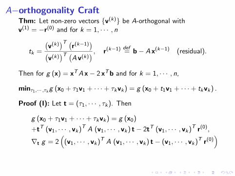
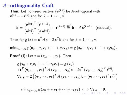
Thm: Let non-zero vectors {v(k)} be A-orthogonal withv(1) = −r(0) and for k = 1, · · · , n
tk =
(v(k)
)T (r(k−1)
)(v(k)
)T (A v(k)
) , r(k−1) def= b− A x(k−1) (residual).
Then for g (x) = xTA x− 2 xTb and for k = 1, · · · , n,
minτ1,··· ,τkg (x0 + τ1v1 + · · ·+ τkvk) = g (x0 + t1v1 + · · ·+ tkvk) .
Proof (I): Let t = (τ1, · · · , τk). Then
g (x0 + τ1v1 + · · ·+ τkvk) = g (x0)
+tT (v1, · · · , vk)T A (v1, · · · , vk) t− 2tT (v1, · · · , vk)T r(0),
∇t g = 2(
(v1, · · · , vk)T A (v1, · · · , vk) t− (v1, · · · , vk)T r(0))
minτ1,··· ,τkg (x0 + τ1v1 + · · ·+ τkvk) ⇐⇒ ∇t g = 0.
A−orthogonality CraftThm: Let non-zero vectors {v(k)} be A-orthogonal withv(1) = −r(0) and for k = 1, · · · , n
tk =
(v(k)
)T (r(k−1)
)(v(k)
)T (A v(k)
) , r(k−1) def= b− A x(k−1) (residual).
Then for g (x) = xTA x− 2 xTb and for k = 1, · · · , n,
minτ1,··· ,τkg (x0 + τ1v1 + · · ·+ τkvk) = g (x0 + t1v1 + · · ·+ tkvk) .
Proof (I): Let t = (τ1, · · · , τk). Then
g (x0 + τ1v1 + · · ·+ τkvk) = g (x0)
+tT (v1, · · · , vk)T A (v1, · · · , vk) t− 2tT (v1, · · · , vk)T r(0),
∇t g = 2(
(v1, · · · , vk)T A (v1, · · · , vk) t− (v1, · · · , vk)T r(0))
minτ1,··· ,τkg (x0 + τ1v1 + · · ·+ τkvk) ⇐⇒ ∇t g = 0.

A−orthogonality Craft
Thm: Let non-zero vectors {v(k)} be A-orthogonal withv(1) = −r(0) and for k = 1, · · · , n
tk =
(v(k)
)T (r(k−1)
)(v(k)
)T (A v(k)
) , r(k−1) def= b− A x(k−1) (residual).
Then for g (x) = xTA x− 2 xTb and for k = 1, · · · , n,
minτ1,··· ,τkg(x0 + τ1v
(1) + · · ·+ τkv(k))
= g(x0 + t1v
(1) + · · ·+ tkv(k)).
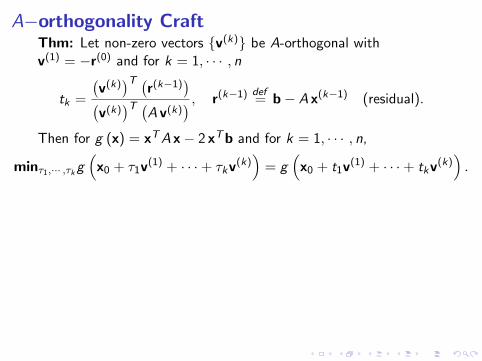
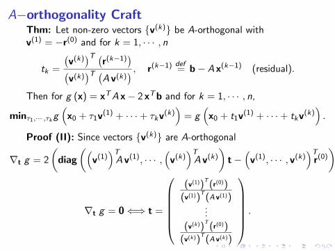
Proof (II): Since vectors {v(k)} are A-orthogonal
∇t g = 2
(diag
((v(1))TA v(1), · · · ,
(v(k)
)TA v(k)
)t−
(v(1), · · · , v(k)
)Tr(0)
).
∇t g = 0⇐⇒ t =
(v(1))
T(r(0))
(v(1))T
(A v(1))...
(v(k))T
(r(0))
(v(k))T
(A v(k))
.
A−orthogonality CraftThm: Let non-zero vectors {v(k)} be A-orthogonal withv(1) = −r(0) and for k = 1, · · · , n
tk =
(v(k)
)T (r(k−1)
)(v(k)
)T (A v(k)
) , r(k−1) def= b− A x(k−1) (residual).
Then for g (x) = xTA x− 2 xTb and for k = 1, · · · , n,
minτ1,··· ,τkg(x0 + τ1v
(1) + · · ·+ τkv(k))
= g(x0 + t1v
(1) + · · ·+ tkv(k)).
Proof (II): Since vectors {v(k)} are A-orthogonal
∇t g = 2
(diag
((v(1))TA v(1), · · · ,
(v(k)
)TA v(k)
)t−
(v(1), · · · , v(k)
)Tr(0)
).
∇t g = 0⇐⇒ t =
(v(1))
T(r(0))
(v(1))T
(A v(1))...
(v(k))T
(r(0))
(v(k))T
(A v(k))
.

A−orthogonality Craft
Thm: Let non-zero vectors {v(k)} be A-orthogonal withv(1) = −r(0) and for k = 1, · · · , n
tk =
(v(k)
)T (r(k−1)
)(v(k)
)T (A v(k)
) , r(k−1) def= b− A x(k−1) (residual).
Then for g (x) = xTA x− 2 xTb and for k = 1, · · · , n,
minτ1,··· ,τkg(x0 + τ1v
(1) + · · ·+ τkv(k))
= g(x0 + t1v
(1) + · · ·+ tkv(k)).
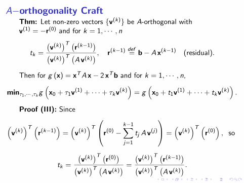
Proof (III): Since
(v(k)
)T (r(k−1)
)=(v(k)
)T r(0) −k−1∑j=1
tj A v(j)
=(v(k)
)T (r(0)), so
tk =
(v(k)
)T (r(0))(
v(k))T (
A v(k)) =
(v(k)
)T (r(k−1)
)(v(k)
)T (A v(k)
) .
A−orthogonality CraftThm: Let non-zero vectors {v(k)} be A-orthogonal withv(1) = −r(0) and for k = 1, · · · , n
tk =
(v(k)
)T (r(k−1)
)(v(k)
)T (A v(k)
) , r(k−1) def= b− A x(k−1) (residual).
Then for g (x) = xTA x− 2 xTb and for k = 1, · · · , n,
minτ1,··· ,τkg(x0 + τ1v
(1) + · · ·+ τkv(k))
= g(x0 + t1v
(1) + · · ·+ tkv(k)).
Proof (III): Since
(v(k)
)T (r(k−1)
)=(v(k)
)T r(0) −k−1∑j=1
tj A v(j)
=(v(k)
)T (r(0)), so
tk =
(v(k)
)T (r(0))(
v(k))T (
A v(k)) =
(v(k)
)T (r(k−1)
)(v(k)
)T (A v(k)
) .
A−orthogonality vectors (I)
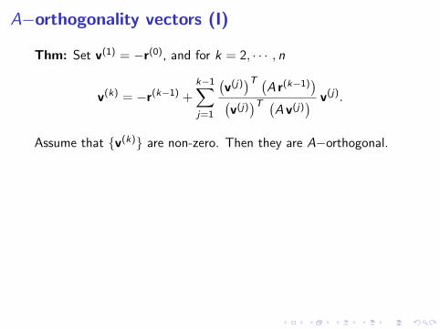
Thm: Set v(1) = −r(0), and for k = 2, · · · , n
v(k) = −r(k−1) +k−1∑j=1
(v(j))T (
A r(k−1))(
v(j))T (
A v(j)) v(j).
Assume that {v(k)} are non-zero. Then they are A−orthogonal.Induction Proof: For all 1 ≤ i < k,(
v(k))T (
A v(i))
= −(r(k−1)
)T (A v(i)
)+
k−1∑j=1
(v(j))T (
A r(k−1))(
v(j))T (
A v(j)) (v(j)
)T (A v(i)
)= −
(r(k−1)
)T (A v(i)
)+(v(i))T (
A r(k−1))
= 0.
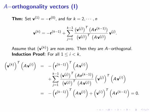
A−orthogonality vectors (I)
Thm: Set v(1) = −r(0), and for k = 2, · · · , n
v(k) = −r(k−1) +k−1∑j=1
(v(j))T (
A r(k−1))(
v(j))T (
A v(j)) v(j).
Assume that {v(k)} are non-zero. Then they are A−orthogonal.
Induction Proof: For all 1 ≤ i < k,(v(k)
)T (A v(i)
)= −
(r(k−1)
)T (A v(i)
)+
k−1∑j=1
(v(j))T (
A r(k−1))(
v(j))T (
A v(j)) (v(j)
)T (A v(i)
)= −
(r(k−1)
)T (A v(i)
)+(v(i))T (
A r(k−1))
= 0.
A−orthogonality vectors (I)
Thm: Set v(1) = −r(0), and for k = 2, · · · , n
v(k) = −r(k−1) +k−1∑j=1
(v(j))T (
A r(k−1))(
v(j))T (
A v(j)) v(j).
Assume that {v(k)} are non-zero. Then they are A−orthogonal.Induction Proof: For all 1 ≤ i < k,(
v(k))T (
A v(i))
= −(r(k−1)
)T (A v(i)
)+
k−1∑j=1
(v(j))T (
A r(k−1))(
v(j))T (
A v(j)) (v(j)
)T (A v(i)
)= −
(r(k−1)
)T (A v(i)
)+(v(i))T (
A r(k−1))
= 0.
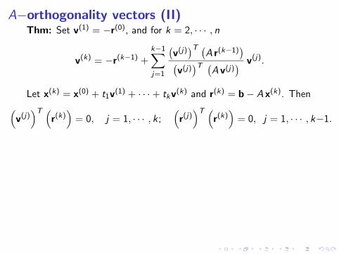
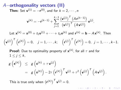
A−orthogonality vectors (II)
Thm: Set v(1) = −r(0), and for k = 2, · · · , n
v(k) = −r(k−1) +k−1∑j=1
(v(j))T (
A r(k−1))(
v(j))T (
A v(j)) v(j).
Let x(k) = x(0) + t1v(1) + · · ·+ tkv(k) and r(k) = b− A x(k). Then(
v(j))T (
r(k))
= 0, j = 1, · · · , k ;(r(j))T (
r(k))
= 0, j = 1, · · · , k−1.
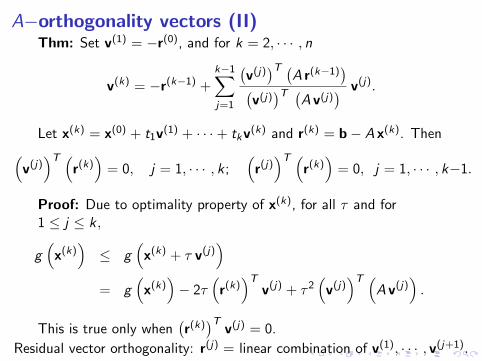
Proof: Due to optimality property of x(k), for all τ and for1 ≤ j ≤ k ,
g(x(k)
)≤ g
(x(k) + τ v(j)
)= g
(x(k)
)− 2τ
(r(k))T
v(j) + τ2(v(j))T (
A v(j)).
This is true only when(r(k))T
v(j) = 0.
Residual vector orthogonality: r(j) = linear combination of v(1), · · · , v(j+1).
A−orthogonality vectors (II)Thm: Set v(1) = −r(0), and for k = 2, · · · , n
v(k) = −r(k−1) +k−1∑j=1
(v(j))T (
A r(k−1))(
v(j))T (
A v(j)) v(j).
Let x(k) = x(0) + t1v(1) + · · ·+ tkv(k) and r(k) = b− A x(k). Then(
v(j))T (
r(k))
= 0, j = 1, · · · , k ;(r(j))T (
r(k))
= 0, j = 1, · · · , k−1.
Proof: Due to optimality property of x(k), for all τ and for1 ≤ j ≤ k ,
g(x(k)
)≤ g
(x(k) + τ v(j)
)= g
(x(k)
)− 2τ
(r(k))T
v(j) + τ2(v(j))T (
A v(j)).
This is true only when(r(k))T
v(j) = 0.
Residual vector orthogonality: r(j) = linear combination of v(1), · · · , v(j+1).

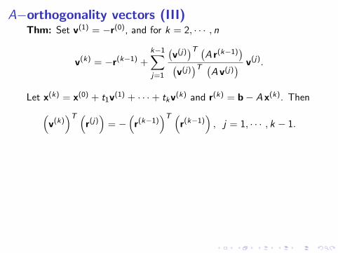
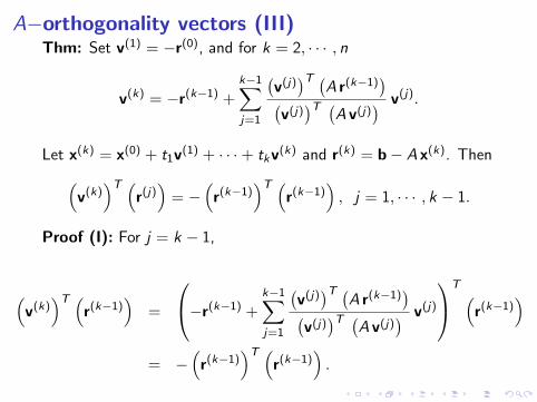
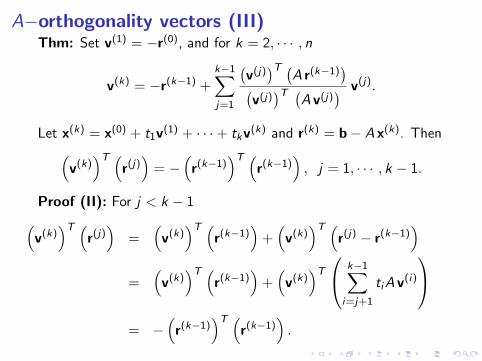
A−orthogonality vectors (III)
Thm: Set v(1) = −r(0), and for k = 2, · · · , n
v(k) = −r(k−1) +k−1∑j=1
(v(j))T (
A r(k−1))(
v(j))T (
A v(j)) v(j).
Let x(k) = x(0) + t1v(1) + · · ·+ tkv(k) and r(k) = b− A x(k). Then(
v(k))T (
r(j))
= −(r(k−1)
)T (r(k−1)
), j = 1, · · · , k − 1.
Proof (I): For j = k − 1,
(v(k)
)T (r(k−1)
)=
−r(k−1) +k−1∑j=1
(v(j))T (
A r(k−1))(
v(j))T (
A v(j)) v(j)
T (r(k−1)
)= −
(r(k−1)
)T (r(k−1)
).
A−orthogonality vectors (III)Thm: Set v(1) = −r(0), and for k = 2, · · · , n
v(k) = −r(k−1) +k−1∑j=1
(v(j))T (
A r(k−1))(
v(j))T (
A v(j)) v(j).
Let x(k) = x(0) + t1v(1) + · · ·+ tkv(k) and r(k) = b− A x(k). Then(
v(k))T (
r(j))
= −(r(k−1)
)T (r(k−1)
), j = 1, · · · , k − 1.
Proof (I): For j = k − 1,
(v(k)
)T (r(k−1)
)=
−r(k−1) +k−1∑j=1
(v(j))T (
A r(k−1))(
v(j))T (
A v(j)) v(j)
T (r(k−1)
)= −
(r(k−1)
)T (r(k−1)
).
A−orthogonality vectors (III)
Thm: Set v(1) = −r(0), and for k = 2, · · · , n
v(k) = −r(k−1) +k−1∑j=1
(v(j))T (
A r(k−1))(
v(j))T (
A v(j)) v(j).
Let x(k) = x(0) + t1v(1) + · · ·+ tkv(k) and r(k) = b− A x(k). Then(
v(k))T (
r(j))
= −(r(k−1)
)T (r(k−1)
), j = 1, · · · , k − 1.
Proof (II): For j < k − 1(v(k)
)T (r(j))
=(v(k)
)T (r(k−1)
)+(v(k)
)T (r(j) − r(k−1)
)=
(v(k)
)T (r(k−1)
)+(v(k)
)T k−1∑i=j+1
tiA v(i)
= −
(r(k−1)
)T (r(k−1)
).
A−orthogonality vectors (III)Thm: Set v(1) = −r(0), and for k = 2, · · · , n
v(k) = −r(k−1) +k−1∑j=1
(v(j))T (
A r(k−1))(
v(j))T (
A v(j)) v(j).
Let x(k) = x(0) + t1v(1) + · · ·+ tkv(k) and r(k) = b− A x(k). Then(
v(k))T (
r(j))
= −(r(k−1)
)T (r(k−1)
), j = 1, · · · , k − 1.
Proof (II): For j < k − 1(v(k)
)T (r(j))
=(v(k)
)T (r(k−1)
)+(v(k)
)T (r(j) − r(k−1)
)=
(v(k)
)T (r(k−1)
)+(v(k)
)T k−1∑i=j+1
tiA v(i)
= −
(r(k−1)
)T (r(k−1)
).

A−orthogonality: A Gift from Math God
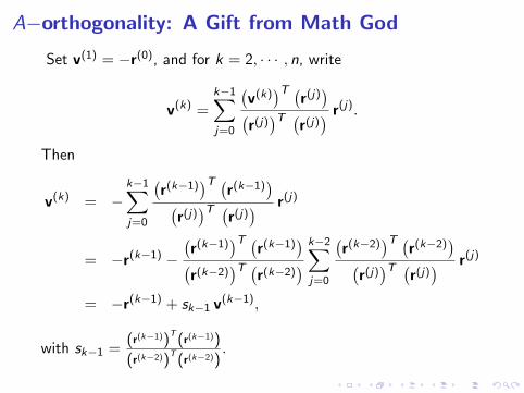
Set v(1) = −r(0), and for k = 2, · · · , n, write
v(k) =k−1∑j=0
(v(k)
)T (r(j))(
r(j))T (
r(j)) r(j).
Then
v(k) = −k−1∑j=0
(r(k−1)
)T (r(k−1)
)(r(j))T (
r(j)) r(j)
= −r(k−1) −(r(k−1)
)T (r(k−1)
)(r(k−2)
)T (r(k−2)
) k−2∑j=0
(r(k−2)
)T (r(k−2)
)(r(j))T (
r(j)) r(j)
= −r(k−1) + sk−1 v(k−1),
with sk−1 =(r(k−1))
T(r(k−1))
(r(k−2))T
(r(k−2)).
A−orthogonality: A Gift from Math God
Set v(1) = −r(0), and for k = 2, · · · , n, write
v(k) =k−1∑j=0
(v(k)
)T (r(j))(
r(j))T (
r(j)) r(j).
Then
v(k) = −k−1∑j=0
(r(k−1)
)T (r(k−1)
)(r(j))T (
r(j)) r(j)
= −r(k−1) −(r(k−1)
)T (r(k−1)
)(r(k−2)
)T (r(k−2)
) k−2∑j=0
(r(k−2)
)T (r(k−2)
)(r(j))T (
r(j)) r(j)
= −r(k−1) + sk−1 v(k−1),
with sk−1 =(r(k−1))
T(r(k−1))
(r(k−2))T
(r(k−2)).
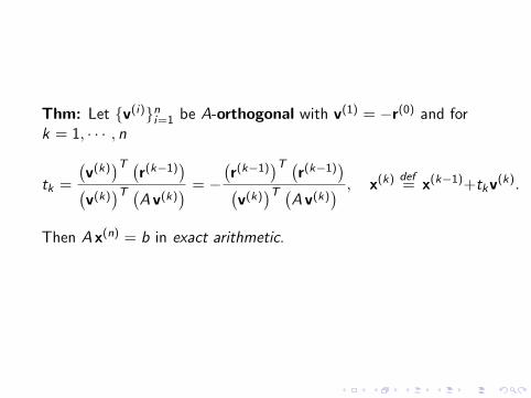
Thm: Let {v(i)}ni=1 be A-orthogonal with v(1) = −r(0) and fork = 1, · · · , n
tk =
(v(k)
)T (r(k−1)
)(v(k)
)T (A v(k)
) = −(r(k−1)
)T (r(k−1)
)(v(k)
)T (A v(k)
) , x(k) def= x(k−1)+tkv
(k).
Then A x(n) = b in exact arithmetic.
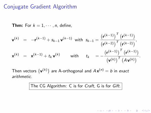
Conjugate Gradient Algorithm
Thm: For k = 1, · · · , n, define,
v(k) = −r(k−1) + sk−1 v(k−1) with sk−1 =
(r(k−1)
)T (r(k−1)
)(r(k−2)
)T (r(k−2)
) ,x(k) = x(k−1) + tk v
(k) with tk = −(r(k−1)
)T (r(k−1)
)(v(k)
)T (A v(k)
) .
Then vectors {v(k)} are A-orthogonal and A x(n) = b in exactarithmetic.
The CG Algorithm: C is for Craft, G is for Gift.
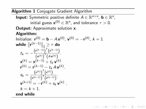
Algorithm 1 Conjugate Gradient Algorithm
Input: Symmetric positive definite A ∈ Rn×n, b ∈ Rn,initial guess x(0) ∈ Rn, and tolerance τ > 0.
Output: Approximate solution x.Algorithm:Initialize: r(0) = b− A x(0), v(0) = −r(0), k = 1while
∥∥r(k−1)∥∥
2≥ τ do
tk = −(r(k−1))T
(r(k−1))
(v(k))T
(A v(k)).
x(k) = x(k−1) + tk v(k)
r(k) = r(k−1) − tk A v(k).
sk =(r(k))
T(r(k))
(r(k−1))T
(r(k−1)).
v(k+1) = −r(k) + sk v(k) .
k = k + 1.end while


![FAST AND ACCURATE COMPUTATION OF GAUSS–LEGENDRE … · In this paper we are concerned with Gauss–Jacobi quadrature, associated with the canonical interval [ −1,1] and the Jacobi](https://img.pdfslide.us/doc/110x75/5ebe8413aab3fe1fe27876f4/fast-and-accurate-computation-of-gaussalegendre-in-this-paper-we-are-concerned.jpg)