04/19/23 330 Lecture 5 1

STATS 330: Lecture 5

04/19/23 330 Lecture 5 2

Tutorials These will cover computing details Held in basement floor tutorial lab,

Building 303 South (303S B75)• Tutorial 1: Wednesday 11-12• Tutorial 2: Friday 10-11 • Tutorial 2: Friday 2-3

Start this Thursday

04/19/23 330 Lecture 5 3

My office hours Tuesday 10:30 – 12:00

Thursday 10:30 – 12:00

Room 265, Building 303S• Come up to the second floor in the Computer

Science lifts, through the doors and turn right

Tutor office hours Tuesday 1-4 pm Thursday 12-2, 3-4 pm Friday 1-3 pm

All in Room 303.133 (First floor, Building 303)

04/19/23 330 Lecture 5 4

Next Week Monday, Thursday lectures by Arden

Miller

No lecture Tuesday

Don’t forget assignment due Aug 4

04/19/23 330 Lecture 5 5

04/19/23 330 Lecture 5 6

Today’s lecture: The multiple regression model

Aim of the lecture: To describe the type of data suitable for

multiple regression To review the multiple regression model To describe some plots that check the

suitability of the model

04/19/23 330 Lecture 5 7

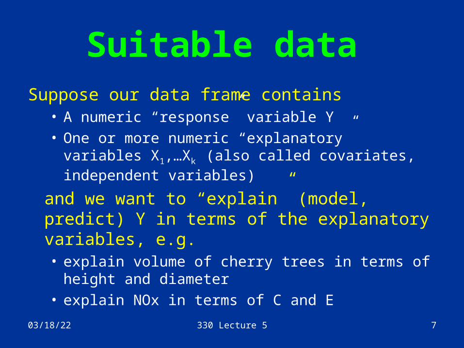
Suitable data Suppose our data frame contains

• A numeric “response” variable Y

• One or more numeric “explanatory” variables X1,…Xk

(also called covariates, independent variables)

and we want to “explain” (model, predict) Y in terms of the explanatory variables, e.g.• explain volume of cherry trees in terms of height and

diameter• explain NOx in terms of C and E

04/19/23 330 Lecture 5 8

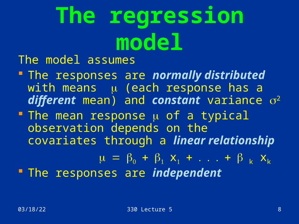
The regression model

The model assumes The responses are normally distributed with

means (each response has a different mean) and constant variance 2

The mean response of a typical observation depends on the covariates through a linear relationship

xk xk

The responses are independent

04/19/23 330 Lecture 5 9

The regression plane

The relationship

xk xk

can be visualized as a plane.

The plane is determined by the coefficients ,k

e.g. for k=2 (k=number of covariates)

04/19/23 330 Lecture 5 10

0

0.2

0.4

0.6

0.8 1

0

0.3

0.6

0.9

-1

-0.5

0

0.5

1

Y

X2

X1

Slope =

slope= 2

0

04/19/23 330 Lecture 5 11

The regression model (cont)

The data is scattered above and below the plane:

Size of “sticks” is random, controlled by 2, doesn’t depend on

x1, x2

aaa

Y

X1

O

X2

04/19/23 330 Lecture 5 12

Alternative form of model

Y

xk xk

where is normally distributed with mean zero and variance 2

04/19/23 330 Lecture 5 13

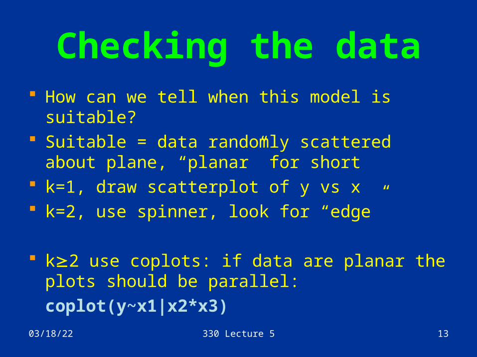
Checking the data How can we tell when this model is suitable? Suitable = data randomly scattered about plane,

“planar” for short k=1, draw scatterplot of y vs x k=2, use spinner, look for “edge”

k2 use coplots: if data are planar the plots should be parallel:

coplot(y~x1|x2*x3)

04/19/23 330 Lecture 5 14

040

80

4 8 12 4 8 12 4 8 12

040

80

040

80

040

80

040

80

4 8 12 4 8 12 4 8 12

040

80

x1

y

-5 0 5 10

Given : x2

12

34

5

Giv

en

: x3

04/19/23 330 Lecture 5 15

Interpretation of coefficients

The regression coefficient 0 gives the average response when all covariates are zero

The regression coefficient 1 • gives the slope of the plane in the x1 direction• measures the average increase in the response for a

unit increase in x1 when all other covariates are held constant

• Is the slope of plots of y versus x1 in a coplot• Is not necessarily the slope of y versus x in a scatter

plot

04/19/23 330 Lecture 5 16

ExampleConsider data from model

y = 5 - 1*x1 + 4*x2 + N(0,1)

x1 and x2 highly correlated, r = 0.95

Regression of y on x1 alone has slope 2.767:

04/19/23 330 Lecture 5 17

Scatter plot: y vs x1

0.0 0.2 0.4 0.6 0.8 1.0

56

78

Slope = 2.767

x1

y

Slope 2.767

04/19/23 330 Lecture 5 18

Coplot

56

78

0.0 0.2 0.4 0.6 0.8 1.0 0.0 0.2 0.4 0.6 0.8 1.0

56

78

0.0 0.2 0.4 0.6 0.8 1.0

56

78

0.0 0.2 0.4 0.6 0.8 1.0

x1

y

0.2 0.4 0.6 0.8 1.0

Given : x2

Slopes are all about - 1

Points to note The regression coefficients 1 and 2 refer to the

conditional mean of the response, given the covariates (in this case conditional on x1 and x2)

1 is the slope in the coplot, conditioning on x2

The coefficient in the plot of y versus x1 refers to a different conditional distribution (conditional on x1 only)

The same if and only if x1 and x2 uncorrelated

04/19/23 330 Lecture 5 19

04/19/23 330 Lecture 5 20

Estimation of the coefficients

We estimate the (unknown) regression plane by the “least squares plane” (best fitting plane)

Best fitting plane = plane that minimizes the sum of squared vertical deviations from the plane

That is, minimize the least squares criterion

2110

1

)...( ikki

n

ii xbxbby

04/19/23 330 Lecture 5 21

Estimation of the coefficients (2)

The R command lm calculates the coefficients of the best fitting plane

This function solves the normal equations, a set of linear equations derived by differentiating the least squares criterion with respect to the coefficients

04/19/23 330 Lecture 5 22

Math Stuff (only if you like it)

Arrange data on response and covariates into a vector y and a matrix X

nkn

k

n xx

xx

y

y

1

1111

1

1

, X y

04/19/23 330 Lecture 5 23

Math Stuff: Normal equations

Estimates are solutions of

yX'XbX'

04/19/23 330 Lecture 5 24

Calculation of best fitting plane

> lm(y~x1+x2)

Call:lm(formula = y ~ x1 + x2)

Coefficients:(Intercept) x1 x2 4.988 -1.055 4.060

x.x - y21

0604055.1988.4 is plane Fitted

04/19/23 330 Lecture 5 25

How well does the plane fit?

Judge this by examining the residuals and fitted values: Each observation has a fitted value:• Yi: response for observation i, xi1, xi2: values of explanatory

variables for observation i

• Fitted plane is

• Fitted value for observation i is

(the height of the fitted plane at (xi1,xi2)

22110ˆˆˆ xxy

22110ˆˆˆˆ iii xxy

04/19/23 330 Lecture 5 26

How well does the plane fit? (cont)

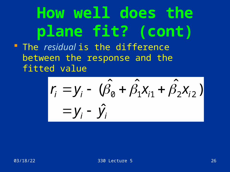
The residual is the difference between the response and the fitted value

ii

iiii

yy

xxyr

ˆ

)ˆˆˆ( 22110

04/19/23 330 Lecture 5 27

How well does the plane fit (cont)

For a good fit, residuals must be• Small relative to the y’s• Have no pattern (don’t depend on the fitted

values, x’s etc)

For the model to be useful, we should have a strong relationship between the response and the explanatory variables

04/19/23 330 Lecture 5 28

Measuring goodness of fit

How can we measure the relative size of residuals and the strength of the relationship between y and the x’s?

The “anova identity” is a way of explaining this

04/19/23 330 Lecture 5 29

Measuring goodness of fit (cont)

Consider the “residual sum of squares”

Provides an overall measure of the size of the residuals

04/19/23 330 Lecture 5 30

Measuring goodness of fit (cont)

Consider the “total sum of squares”

Provides an overall measure of the variability of the data

04/19/23 330 Lecture 5 31

Math stuff: ANOVA identity

Math result: Anova Identity

TSS = RegSS + RSS

Since RegSS is non-negative, RSS must be less than

TSS so RSS/TSS is between 0 and 1.

2

1

2

1

2

1

)ˆ()ˆ()( i

n

ii

n

ii

n

ii yyyyyy

RegSS: Regression sum of squares

04/19/23 330 Lecture 5 32

Interpretation The smaller RSS compared to TSS, the

better the fit. If RSS is 0, and TSS is positive, we have a

perfect fit If RegSS=0, RSS=TSS and the plane is

flat (all coefficients except the constant are zero) , so the x’s don’t help predict y

04/19/23 330 Lecture 5 33

R2

Another way to express this is the coefficient of determination R2

This is defined as 1-RSS/TSS = RegSS/TSS

R2 is always between 0 and 1• 1 means a perfect fit• 0 means a flat plane

R2 is the square of the correlation between the observations and the fitted values

04/19/23 330 Lecture 5 34

Estimate of

Recall that controls the scatter of the observations about the regression plane:• the bigger , the more scatter• the bigger , the smaller R2

estimated by

s2=RSS/(n-k-1)

04/19/23 330 Lecture 5 35

Calculationscherry.lm <- lm(volume~diameter+height,

data=cherry.df))

summary(cherry.lm)

The lm function produces an “lm object” that contains all the information from fitting the regression

lm = “linear model”

“ell” not I !!!!

04/19/23 330 Lecture 5 36

Call:lm(formula = volume ~ diameter + height, data = cherry.df)

Residuals: Min 1Q Median 3Q Max -6.4065 -2.6493 -0.2876 2.2003 8.4847

Coefficients: Estimate Std. Error t value Pr(>|t|) (Intercept) -57.9877 8.6382 -6.713 2.75e-07 ***diameter 4.7082 0.2643 17.816 < 2e-16 ***height 0.3393 0.1302 2.607 0.0145 * ---Signif. codes: 0 `***' 0.001 `**' 0.01 `*' 0.05 `.' 0.1 ` ' 1

Residual standard error: 3.882 on 28 degrees of freedomMultiple R-Squared: 0.948, Adjusted R-squared: 0.9442 F-statistic: 255 on 2 and 28 DF, p-value: < 2.2e-16

Info on residuals

coefficients

R2

Estimate of

Cherries