Appendix

A.1 Further Monographs

In the following, monographs are listed, which are recommended for a furtherstudy. The selection is limited to micrometeorological and measurement techniquetextbooks.

Further Micrometeorological Literature

Arya, SP (1999) Air pollution meteorology and dispersion. Oxford University Press, New York,Oxford, 310 pp.

Arya, SP (2001) Introduction to micrometeorology. Academic Press, San Diego, 415 pp.Bailey, WG, Oke, TR, Rouse, WR (eds) (1997) The surface climate of Canada. Mc Gill-Queen's

University Press, Montreal, Kingston, 369 pp.Barry R and Blanken P (2016) Microclimate and local climate. Cambridge University Press,

Cambridge, 379 pp.Bendix, J (2004) Geländeklimatologie. Borntraeger, Berlin, Stuttgart, 282 pp.Bird RB, Stewart WE and Lightfoot EN (2007) Transport phenomena. John Wiley & Sons, Inc.,

New York, 905 pp.Blackadar, AK (1997) Turbulence and diffusion in the atmosphere. Springer, Berlin, Heidelberg,

185 pp.Campbell GS and Norman JM (2013) Introduction to environmental biophysics. Springer, New

York, 312 pp.Garratt, JR (1992) The atmospheric boundary layer. Cambridge University Press, Cambridge,

316 pp.Geiger R, Aron RH and Todhunter P (2009) The Climate near the ground. Rowman & Littlefield,

Lanham, XVIII, 623 pp.Hari P, Heliövaara K and Kulmala L (eds) (2013) Physical and physiological forest ecology.

Springer, Dordrecht, Heidelberg, New York, London, 534 pp.Hatfield JL and Baker JM (eds) (2005) Micrometeorology in agricultural systems. American

Society of Agronomy, Madison, 584 pp.Jones HG (2013) Plants and microclimate. Cambridge Univ. Press, Cambridge, 423 pp.Kaimal, JC, Finnigan, JJ (1994) Atmospheric boundary layer flows: Their structure and

measurement. Oxford University Press, New York, NY, 289 pp.

© Springer-Verlag Berlin Heidelberg 2017T. Foken, Micrometeorology, DOI 10.1007/978-3-642-25440-6

327

Kantha, LH, Clayson, CA (2000) Small scale processes in geophysical fluid flows. AcademicPress, San Diego, 883 pp.

Kraus H (2008) Grundlagen der Grenzschichtmeteorologie. Springer, Berlin, Heidelberg, 211 pp.Leclerc MY and Foken T (2014) Footprints in micrometeorology and ecology. Springer,

Heidelberg, New York, Dordrecht, London, 239 pp.Lee, X, Massman, WJ, Law, B (Editors) (2004) Handbook of micrometeorology: A guide for

surface flux measurement and analysis. Kluwer, Dordrecht, 250 pp.Moene AF and van Dam JC (2014) Transport in the atmosphere-vegetation-soil continuum.

Cambridge University Press, Cambridge, 436 pp.Mölders N (2012) Land-use and land-cover changes, Impact on climate and air quality. Springer,

Dordrecht, Heidelberg, London, New York, 189 pp.Mölders N and Kramm G (2014) Lectures in meteorology. Springer, Cham Heidelberg New York

Dordrecht London 591 pp.Monson R and Baldocchi D (2014) Terrestrial biosphere-atmosphere fluxes. Cambridge University

Press, New York, 487 pp.Monteith JL and Unsworth MH (2008) Principles of environmental physics, 3rd edition. Elsevier,

Academic Press, Amsterdam, Boston, 418 pp.Oke, TR (1987) Boundary layer climates. Methuen, New York, 435 pp.Salby ML (2012) Physics of the atmosphere and climate. Cambridge University Press, Cambridge,

666 pp.Stull, RB (1988) An Introduction to boundary layer meteorology. Kluwer Acad. Publ., Dordrecht,

Boston, London, 666 pp.Stull R (2015) Practical meteorology: An algebra-based survey of atmospheric science. © Author,

CC Attribution 4.0 License, ISBN 978-0-88865-176-1, Vancouver, 924 pp.Venditti JG, Best JL, Church M and Hardy RJ (2013) Coherent flow structures at Earth’s surface.

John Wiley & Sons, Ltd., Chichester, 387 pp.Vilà-Guerau de Arellano J, Van Heerwaarden CC, van Stratum BJH and van den Dries K (2015)

Atmospheric boundary layer. Cambridge University Press, Cambridge, 265 pp.Wyngaard JC (2010) Turbulence in the atmosphere. Cambridge University Press, Cambridge,

393 pp.

Further Measurement Technique LiteratureAubinet M, Vesala T u. Papale D (eds.) (2012) Eddy covariance: A practical guide to measurement

and Data Analysis. Springer, Dordrecht, Heidelberg, London, New York, 438 pp.Bentley, JP (2005) Principles of measurement systems. Pearson Prentice Hall, Harlow, 528 pp.Brock, FV, Richardson, SJ (2001) Meteorological measurement systems. Oxford University Press,

New York, 290 pp.DeFelice, TP (1998) An introduction to meteorological Instrumentation and measurement. Prentice

Hall, Upper Saddle River, 229 pp.Dobson, F, Hasse, L, Davis, R (Editors) (1980) Air-sea interaction, Instruments and methods.

Plenum Press, New York, 679 pp.Emeis S (2010) Measurement methods in atmospheric sciences. Borntraeger Science Publishers,

Stuttgart, 257 pp.Hebra AJ (2010) The physics of metrology. Springer, Wien, New York 383 pp.Harrison GR (2015) Meteorological measurements and instrumentations. John Wiley and Sons,

Chichester, 257 pp.Kaimal, JC, Finnigan, JJ (1994) Atmospheric boundary layer flows: Their structure and

measurement. Oxford University Press, New York, NY, 289 pp.Strangeways I (2003) Measuring the natural environment. 2nd ed. Cambridge University Press,

Cambridge, 534 pp.

328 Further Micrometeorological Literature

A.2 Use of SI-Units

The following table includes important SI-units used in the book. The basic unitsare bold highlighted.

Name SI-unit Unit Calculation

Length Meter mTime Second sVelocity m s−1 1 km h−1 = (1/3.6) m s−1

Acceleration m s−2

Mass Kilogram kgDensity kg m−3

Impulse kg m s−1 1 kg m s−1 = 1 N s

Force Newton N 1 N = 1 kg m s−2

Pressure, friction Pascal Pa 1 Pa = 1 N m−2

1 Pa = 1 kg m−1 s−2

Air pressure Hektopascal hPa 1 hPa = 100 Pa

Work, energy Joule J 1 J = 1 N m = 1 W s1 J = 1 kg m2 s−2

Power Watt W 1 W = 1 J s−1 = 1 N m s−1

1 W = 1 kg m2 s−3

Energy flux density W m−2 1 W m−2 = 1 kg s−3

Temperature Kelvin KCelsius-temperature °C 0 °C = 273.15 K

Temperature difference K

A.3 Constants and Important Parameters

Even though the accuracy of meteorological measurements is at most only 3–5significant digits, the following physical constants are given with errors expressedin ppm, because sometimes in the literature different values are reported.

The values listed are taken from the 1986 calculations of Cohen and Taylor(1986) and the international temperature scale ITS-90 as given by Sonntag (1990).

Constant Symbol Value Error

Standard values

Standard air pressure p0 1013.25 hPa

Standard temperature T0 273.15 K = 0 °C

Temperature of the triple point of water 273.16 K

g 9.80665 m s−2

(continued)

Appendix 329

(continued)

Constant Symbol Value Error

Standard acceleration due to gravity atlatitude 45°

General constants

Velocity of the light in vacuum c 299 792 458 m s−1 Exact

Planck’s constant h 6.626 0755(40) 10−34 J s 0.60

Physical-chemical constants

Avogadro number NA 6.022 1367(36) 1023

mol−10.59

Atom mass 12C/12 mu 1.660 5402(10) 10−27 kg 0.59

Universal gas constant R 8.314 510(70) J mol−1

K−18.4

Boltzmann constant R/NA k 1.380 658(12) J K−1 8.4

Molar volume (ideal gas) RT0/p0 22.414 10(19) l mol−1 8.4

Stefan-Boltzmann constant rSB 5.670 51(19) 10−8 W m−2

K−434

Wien’s constant kmaxT 2.897 756(24) 10−3 m K 8.4

Thermo-dynamical constants

Molar mass of dry air ML 0.028 9645(5) kg mol−1 17

Molar mass of water vapor MW 0.018 01528(50)kg mol−1

27

Ratio MW/ML c 0.62198(2) 33

Gas constant of dry air RL 287.058 6(55) J kg−1 K−1 19

Gas constant of water vapor RW 461.525 (13) J kg−1 K−1 29

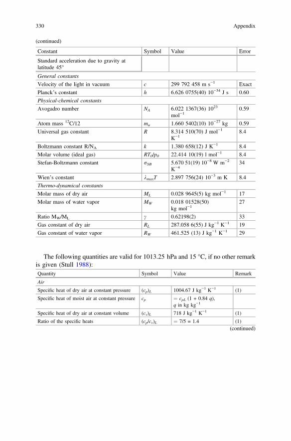
The following quantities are valid for 1013.25 hPa and 15 °C, if no other remarkis given (Stull 1988):Quantity Symbol Value Remark

Air

Specific heat of dry air at constant pressure (cp)L 1004.67 J kg−1 K−1 (1)

Specific heat of moist air at constant pressure cp ¼ cpL (1 + 0.84 q),q in kg kg−1

Specific heat of dry air at constant volume (cv)L 718 J kg−1 K−1 (1)

Ratio of the specific heats (cp/cv)L ¼ 7/5 = 1.4 (1)(continued)

330 Appendix

(continued)

Quantity Symbol Value Remark

Ratio of the gas constant and the specific heatfor dry air

(RL/cp)L ¼ 2/7 = 0.286 (1)

Density qLqL0

1.225 kg m−3

1.2923 kg m−3 � 0 °C(1)

Kinematic molecular viscosity t 1.461 10−5 m2 s−1

Molecular thermal conductivity tT 2.06 10−5 m2 s−1

Molecular Prandtl number Pr 0.7092

Dynamic molecular viscosity µ = qL/t 1.789 10−5 kg m−1 s

Molecular thermal diffusivity aT =tT � qL � cpL

2.53 10−2 W m−1 K−1

Psychrometric constant (water) 6.53 10−4 (1 +0.000944 t‘) p K−1

(2)

Psychrometric constant (ice) 5,75 10−4p K−1 (2)

Water and water vapor

Specific heat of water vapor at constantpressure

(cp)W 1846 J kg−1 K−1

Specific heat of water vapor at constantvolume

(cv)W 1389 J kg−1 K−1

Ratio of the specific heats (cp/cv)W ¼ 4/3 = 1.333

Ratio of the gas constant and the specific heat (RL/cp)W ¼ 1/4 = 0.25

Density of water qW 999.84 kg m−3 (0 °C,1000 hPa)

(3)

Latent heat of vaporization k (2.501 − 0.00237 t) 106

J kg−1

Other quantities

Coriolis parameter f 1.458 10−4 sin u s−1 (1)

Solar constant S energy units:−1361 W m−2

kinematic units:−1.119 K m s−1

(4)

Constant gravity acceleration g0 9.81 m s−2 (5)

(1) identical data in Landolt-Börnstein (Fischer 1988) according to WMO recommendations(2) Sonntag (1990)(3) Wagner and Pruß (2002)(4) Kopp and Lean (2011)(5) Hantel (2013)

Temperature dependent quantities (Fischer 1988)

Temperature Specific heatcapacity in 103

J kg−1 K−1

Latent heat in 106 J kg−1

Ice Water Vaporization Fusion Sublimation

−20 1.959 4.35 2.5494 0.2889 2.8387(continued)

Appendix 331

(continued)

Temperature Specific heatcapacity in 103

J kg−1 K−1

Latent heat in 106 J kg−1

Ice Water Vaporization Fusion Sublimation

−10 2.031 4.27 2.5247 0.3119 2.8366

0 2.106 4.2178 2.50084 0.3337 2.8345

5 4.2023 2.4891

10 4.1923 2.4774

15 4.1680 2.4656

20 4.1818 2.4535

25 4.1797 2.4418

30 4.1785 2.4300

35 4.1780 2.4183

40 4.1785 2.4062

A.4 Further Equations

Calculation of Astronomical Quantities

In some applications, it is often necessary to determine the solar inclination angle asa function of time. The following approximations for some of these calculationsmust be applied in several steps:

To determine the declination of the sun,d, the latitude of the sun, us, must first becalculated (Sonntag 1989; VDI 2015)

uS ¼ x� 77:51� þ 1:92� � sin xx ¼ 0:9856� � DOY � 2:72�

ðA:1Þ

where DOY is the day of the year where the 1st of January has the number 1.The declination is given by:

sin d ¼ 0:3978 sinuS ðA:2Þ

To determine the position of the sun, the hour angle x

x ¼ LTST � 12hð Þ � 15� in � ðA:3Þ

must be calculated which gives the angular difference between d and the zenith ofthe sun (Liou 1992), thereby LTST is the local true solar time. It is necessary to

332 Appendix

apply the equation of time Z (Hughes et al. 1989), which gives the differencebetween the local true and the mean solar time (x see Eq. A.1).

Z ¼ �7:66 sin x� 9:87 sinð2xþ 24:99� þ 3:83� sin xÞ in min ðA:4Þ

The time distance to culmination of the sun, tH, for Central European Time(k = 15°) is given by

tH ¼ t � 12þ Z þ 15� kð Þ460

� �� �3600; ðA:5Þ

where t: time in hours, and k is longitude.With the latitude u in radians of a location, the angle of inclination of the sun

can be determined for any time:

sin c ¼ sin d � sin uþ cos d � cos u � cos x ðA:6Þ

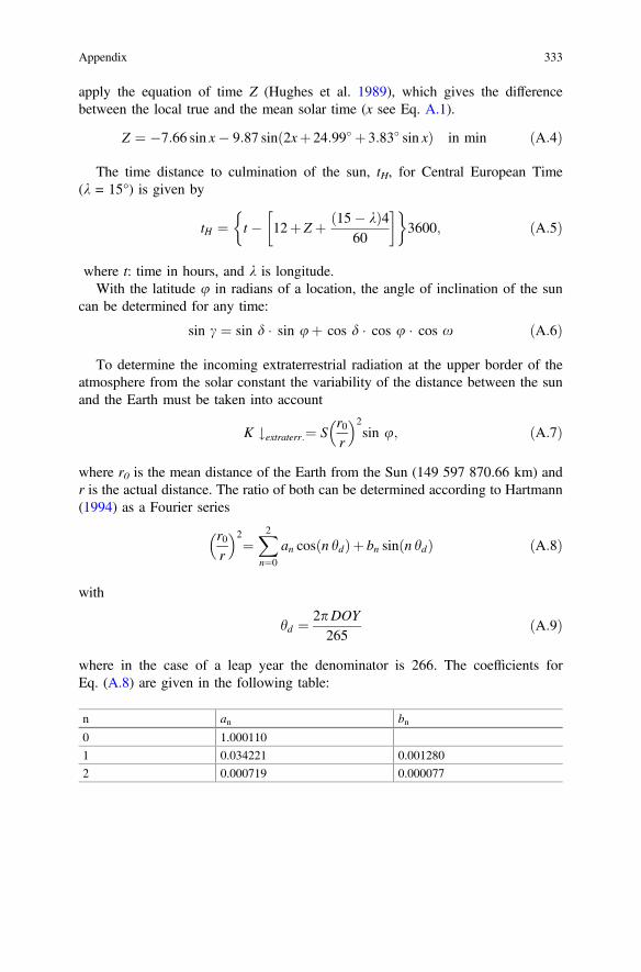
To determine the incoming extraterrestrial radiation at the upper border of theatmosphere from the solar constant the variability of the distance between the sunand the Earth must be taken into account

K #extraterr:¼ Sr0r

� �2sin u; ðA:7Þ

where r0 is the mean distance of the Earth from the Sun (149 597 870.66 km) andr is the actual distance. The ratio of both can be determined according to Hartmann(1994) as a Fourier series

r0r

� �2¼

X2n¼0

an cos n hdð Þþ bn sin n hdð Þ ðA:8Þ

with

hd ¼ 2pDOY265

ðA:9Þ

where in the case of a leap year the denominator is 266. The coefficients forEq. (A.8) are given in the following table:

n an bn0 1.000110

1 0.034221 0.001280

2 0.000719 0.000077

Appendix 333

Universal Functions

Even though the universal function formulated by Businger et al. (1971) and latermodified by Högström (1988) are widely used, knowledge of other universalfunctions may be quite useful for different research activities. The following table isbased on works of Dyer (1974), Yaglom (1977), Foken (1990), and Andreas(2002). The values the von-Kármán constant, j, used in the formulations are given.The notation, 0.40*, indicates that the original function was re-calculated byHögström (1988) using j = 0.40.

Reference j Universal function for momentum exchange

Swinbank (1964) – zL 1� ez=L� �1

z=L\0

Swinbank (1968) 0.40 0:613 �z=Lð Þ�0:2 �0:1� z=L� � 2

Tschalikov (1968) 0.40 1þ 7:74z=L z=L[ 0:04

Zilitinkevich and Tschalikov(1968)

0.434 1þ 1:45z=L � 0:15\z=L\0

0:41 �z=Lð Þ�1=3 �1:2\z=L\� 0:15

1þ 9:9 z=L 0\z=L

0.40* 1þ 1:38z=L � 0:15\z=L\0

0:42 �z=Lð Þ�1=3 �1:2\z=L\� 0:15

1þ 9:4 z=L 0\z=L

Webb (1970) – 1þ 4:5 z=L z=L\� 0:03

Dyer and Hicks (1970) 0.41 1� 16 z=Lð Þ�1=4 �1\z=L\0

Businger et al. (1971) 0.35 1� 15 z=Lð Þ�1=4 �2\z=L\0

1þ 4:7 z=L 0\z=L\1

0.40* 1� 19; 3 z=Lð Þ�1=4 �2\z=L\0

1þ 6 z=L 0\z=L\1

Dyer (1974) 0.41 1� 16 z=Lð Þ�1=4 �1\z=L\0

1þ 5 z=L 0\z=L

0.40* 1� 15:2 z=Lð Þ�1=4 �1\z=L\0

1þ 4:8 z=L 0\z=L

Skeib (1980), see also: Fokenand Skeib (1983) and Foken(1990)

0.400.40*

1 � 0:0625\z=L\0:125

z=L�0:0625

��1=4

�2\z=L\� 0:0625

z=L0:125

0:125\z=L\2

Gavrilov and Petrov (1981) 0.40 1� 8 z=Lð Þ�1=3 z=L\0

1þ 5 z=L 0\z=L

Dyer and Bradley (1982) 0.400.40*

1� 28 z=Lð Þ�1=4 z=L\0

(continued)

334 Appendix

(continued)

Reference j Universal function for momentum exchange

Beljaars and Holtslag (1991) 0.40 1þ z=Lþ 23z=L 6� 0:35z=Lð Þ � e�0:35z=L 0\z=L

King et al. (1996) 0.40 1þ 5:7 z=L� 12 0\z=L

Handorf et al. (1999) 0.40 1þ 5 z=L 0\z=L\0:64 0:6\z=L

Reference j Universal function for the exchange of sensible heat,Prt = 1

Swinbank (1968) 0.40 0:227 �z=Lð Þ�0:44 �0:1� z=L� � 2

Tschalikov (1968) 0.40 1þ 5:17 z=L z=L[ 0:04

Zilitinkevich and Tschalikov(1968)

0.434 1þ 1:45 z=L � 0:15\z=L\0

0:41 �z=Lð Þ�1=3 �1:2\z=L\� 0:15

1þ 9:9 z=L 0\z=L

0.40* 0:95þ 1:31 z=L � 0:15\z=L\0

0:40 �z=Lð Þ�1=3 �1:2\z=L\� 0:15

0:95þ 8:9 z=L 0\z=L

Webb (1970) – 1þ 4:5 z=L z=L\� 0:03

Dyer and Hicks (1970) 0.41 1� 16 z=Lð Þ�1=2 �1\z=L\0

Businger et al. (1971) 0.35 0:74 1� 9 z=Lð Þ�1=2 �2\z=L\0

0:74þ 4:7 z=L 0\z=L\1

0.40* 0:95 1� 11:6 z=Lð Þ�1=2 �2\z=L\0

0:95þ 7:8 z=L 0\z=L\1

Dyer (1974) 0.41 1� 16 z=Lð Þ�1=2 �1\z=L\0

1þ 5 z=L 0\z=L

0.40* 0:95 1� 15:2 z=Lð Þ�1=2 �1\z=L\00:95þ 4:5 z=L 0\z=L

Skeib (1980), see also: Foken andSkeib (1983) and Foken (1990)

0.40 1 �0:0625\z=L\0:125z=L

�0:0625

� ��1=2�2\z=L\� 0:0625

z=L0:125

� �20:125\z=L\2

0.40* 0:95 �0:0625\z=L\0:125

0:95 z=L�0:0625

� ��1=2�2\z=L\� 0:0625

0:95 z=L0:125

� �20:125\z=L\2

Gavrilov and Petrov (1981) 0.400:65 1� 35 z=Lð Þ�1=2 þ 0:25

1þ 8 z=Lð Þ2" #

z=L\0

0:9þ 6 z=L 0\z=L

(continued)

Appendix 335

(continued)

Reference j Universal function for the exchange of sensible heat,Prt = 1

Dyer and Bradley (1982) 0.400.40*

1� 14 z=Lð Þ�1=2 z=L\0

Beljaars and Holtslag (1991) 0.401þ z=L 1þ 2

3z=L

� �1=2þ 2

3z=L 6� 0:35z=Lð Þ e�0:35z=L

0\z=L

King et al. (1996) 0.40 0:95þ 4:99 z=L� 12 0\z=L

Handorf et al. (1999) 0.40 1þ 5 z=L 0\z=L\0:64 0:6\z=L

Reference j Universal function for the energy dissipation

Wyngaard and Coté (1971) 0.351þ 0:5 z=Lj j2=3h i3=2

z=L\0

1þ 2:5 z=Lð Þ3=5h i3=2

z=L[ 0

Högström (1990) 1:24 1� 19 z=Lð Þ�1=4� zL

h iz=L\0

1:24þ 4:7z=L z=L[ 0

Thiermann and Graßl(1992)

1� 3z=Lð Þ�1�z=L z=L\0

1þ 4z=Lþ 16 z=Lð Þ2h i�1=2

z=L[ 0

Kaimal and Finnigan(1994) 1þ 0:5 z=Lj j2=3

h i3=2z=L\0

1þ 5z=L z=L[ 0

Frenzen and Vogel (2001) 0:85 1� 16z=Lð Þ�2=3�z=Lh i

z=L\0

0:85þ 4:26z=Lþ 2:58 � z=Lð Þ2 z=L[ 0

Hartogensis and DeBruin(2005)

0:8þ 2:5 � z=L z=L[ 0

Reference j Universal function for the temperature structurefunction parameter

Wyngaard et al. (1971),Wyngaard (1973)

0.35 4:9 1� 7z=Lð Þ�2=3 z=L\0

4:9 1þ 2:4 z=Lð Þ2=3h i

z=L[ 0

0.40** 4:9 1� 6:1z=Lð Þ�2=3 z=L\0

4:9 1þ 2:2 z=Lð Þ2=3h i

z=L[ 0

Foken and Kretschmer (1990) 0.40 ð0:95=jÞ2 1� 11:6 z=Lð Þ�1=2 �2\z=L\00:95=j2 0:95þ 7:8 z=Lð Þ 0\z=L\1

(continued)

336 Appendix

(continued)

Reference j Universal function for the temperature structurefunction parameter

Thiermann and Graßl (1992)6:34 1� 7z=Lþ 75 z=Lð Þ2

h i�1=3z=L\0

6:34 1� 7z=Lþ 20 z=Lð Þ2h i1=3

z=L[ 0

Kaimal and Finnigan (1994) 5 1þ 6:4 z=Lj jð Þ�2=3 z=L\04 1þ 3z=Lð Þ z=L\0

Hartogensis and DeBruin(2005)

4:7 1þ 1:6 z=Lð Þ2=3h i

z=L[ 0

Li et al. (2012) 6:7 1� 14:9z=Lð Þ�2=3 z=L\0

4:5 1þ 1:3 z=Lð Þ2=3h i

z=L[ 0

Maronga (2013) 6:1 1� 7:6z=Lð Þ�2=3 z=L\0

Braam et al. (2014) 4:4 1� 10:2z=Lð Þ�2=3 �76\z=L\� 0:0075

Integral Turbulence Characteristics in the Surface Layer

Reference ru=u� rv=u� Stratification

Lumley and Panofsky (1964),Panofsky and Dutton (1984)

2.45 1.9 Neutral, unstable

McBean (1971) 2.2 1.9 Unstable

Beljaars et al. (1983) 2.0 1.75 Unstable

Sorbjan (1986) 2.3 Stable

Sorbjan (1987) 2.6

Foken et al. (1991) 2:7

4:15 z=Lð Þ1=8� 0:032\z=L\0

z=L\� 0:032

Thomas and Foken (2002) 0:44 ln 1m fu�

� �þ 3:1 �0:2\z=L\0:4

Reference rw=u� rT=T� Stratification

Lumley and Panofsky (1964),Panofsky and Dutton ((1984)

1.45 Neutral, unstable

McBean (1971) 1.4 1.6 Unstable

Panofsky et al. (1977) 1:3 1� 2z=Lð Þ1=3 Unstable

Caughey u. Readings (1975) z=Lð Þ�1=3 Unstable

Hicks (1981) 1:25 1� 2z=Lð Þ1=3 0:95 z=Lð Þ�1=3 Unstable

(continued)

Appendix 337

(continued)

Reference rw=u� rT=T� Stratification

Caughey and Readings (1975) z=Lð Þ�1=3 Unstable

Beljaars et al. (1983) 0:95 z=Lð Þ�1=3 Unstable

Sorbjan (1986) 1.6 2.4 Stable

Sorbjan (1987) 1.5 3.5 Stable

Foken et al. (1991) 1:3

2:0 z=Lð Þ1=8� 0:032\z=L\0

z=L\� 0:032

Foken et al. (1991; 1997) 1:4 z=Lð Þ�1=4

0:5 z=Lð Þ�1=2

z=Lð Þ�1=4

z=Lð Þ�1=3

0:02\z=L\1

� 0:062\z=L\0:02

� 1\z=L\� 0:062

z=L\� 1

Thomas and Foken (2002) 0:21 ln 1m�fu�

� �þ 6:3 �0:2\z=L\0:4

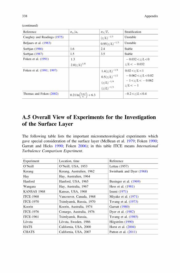
A.5 Overall View of Experiments for the Investigationof the Surface Layer

The following table lists the important micrometeorological experiments whichgave special consideration of the surface layer (McBean et al. 1979; Foken 1990;Garratt and Hicks 1990; Foken 2006); in this table ITCE means InternationalTurbulence Comparison Experiment.

Experiment Location, time Reference

O’Neill O’Neill, USA, 1953 Lettau (1957)

Kerang Kerang, Australien, 1962 Swinbank and Dyer (1968)

Hay Hay, Australien, 1964

Hanford Hanford, USA, 1965 Businger et al. (1969)

Wangara Hay, Australia, 1967 Hess et al. (1981)

KANSAS 1968 Kansas, USA, 1968 Izumi (1971)

ITCE-1968 Vancouver, Canada, 1968 Miyake et al. (1971)

ITCE-1970 Tsimlyansk, Russia, 1970 Tsvang et al. (1973)

Koorin Koorin, Australia, 1974 Garratt (1980)

ITCE-1976 Conargo, Australia, 1976 Dyer et al. (1982)

ITCE-1961 Tsimlyansk, Russia, Tsvang et al. (1985)

Lövsta Lövsta, Sweden, 1986 Högström (1990)

HATS California, USA, 2000 Horst et al. (2004)

CHATS California, USA, 2007 Patton et al. (2011)

338 Appendix

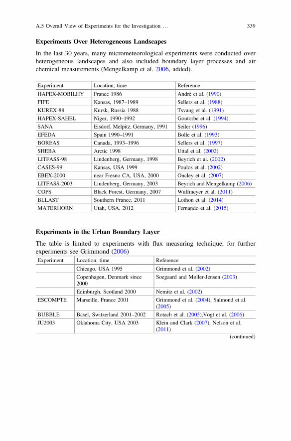
Experiments Over Heterogeneous Landscapes

In the last 30 years, many micrometeorological experiments were conducted overheterogeneous landscapes and also included boundary layer processes and airchemical measurements (Mengelkamp et al. 2006, added).

Experiment Location, time Reference

HAPEX-MOBILHY France 1986 André et al. (1990)

FIFE Kansas, 1987–1989 Sellers et al. (1988)

KUREX-88 Kursk, Russia 1988 Tsvang et al. (1991)

HAPEX-SAHEL Niger, 1990–1992 Goutorbe et al. (1994)

SANA Eisdorf, Melpitz, Germany, 1991 Seiler (1996)

EFEDA Spain 1990–1991 Bolle et al. (1993)

BOREAS Canada, 1993–1996 Sellers et al. (1997)

SHEBA Arctic 1998 Uttal et al. (2002)

LITFASS-98 Lindenberg, Germany, 1998 Beyrich et al. (2002)

CASES-99 Kansas, USA 1999 Poulos et al. (2002)

EBEX-2000 near Fresno CA, USA, 2000 Oncley et al. (2007)

LITFASS-2003 Lindenberg, Germany, 2003 Beyrich and Mengelkamp (2006)

COPS Black Forest, Germany, 2007 Wulfmeyer et al. (2011)

BLLAST Southern France, 2011 Lothon et al. (2014)

MATERHORN Utah, USA, 2012 Fernando et al. (2015)

Experiments in the Urban Boundary Layer

The table is limited to experiments with flux measuring technique, for furtherexperiments see Grimmond (2006)Experiment Location, time Reference

Chicago, USA 1995 Grimmond et al. (2002)

Copenhagen, Denmark since2000

Soegaard and Møller-Jensen (2003)

Edinburgh, Scotland 2000 Nemitz et al. (2002)

ESCOMPTE Marseille, France 2001 Grimmond et al. (2004), Salmond et al.(2005)

BUBBLE Basel, Switzerland 2001–2002 Rotach et al. (2005),Vogt et al. (2006)

JU2003 Oklahoma City, USA 2003 Klein and Clark (2007), Nelson et al.(2011)

(continued)

A.5 Overall View of Experiments for the Investigation … 339

(continued)

Experiment Location, time Reference

Helsinki, Finland 2005–2006 Vesala et al. (2008)

London, England 2008–2011 Kotthaus and Grimmond (2012)

Oberhausen, Germany2010–2011

Goldbach and Kuttler (2013)

Other Experiments Referred to in the Text

The following table gives some information about further experiments mentioned inthis book.

Experiment Location, time Reference

Greenland Greenland, summer 1991 Ohmura (1992)

FINTUREX Neumayer station, Antarktica, Jan.–Febr. 1994

Foken (1996), Handorf et al.(1999)

LINEX-96/2 Lindenberg, Germany, June 1996 Foken et al. (1997)

LINEX-97/1 Lindenberg, Germany, June 1997 Foken (1998)

WALDATEM-2003 Waldstein, Germany, May–July 2003 Thomas and Foken (2007)

EGER Waldstein, Germany 2007, 2008,2011

Foken et al. (2012b)

A.6 Meteorological Measurements Stations

In Sect. 6.2, different types of meteorological measurements stations were defined(Table 6.1). The measured parameters of these stations (VDI 2006) are given in thefollowing table, where X indicates necessary parameters and o indicates desirableadditional parameters. The measured parameters include air temperature (ta), airmoisture (fa), wind velocity (u), wind direction (dd), precipitation (RN), globalradiation (G), net radiation (Qs*), air pressure (p), state of the weather (ww), surfacetemperature (tIR), photosynthetic active radiation (PAR), soil temperature (tb), soilmoisture (fb), soil heat flux (QG), sensible heat flux (QH), latent heat flux (QE),deposition (Qc), shear stress (s).

The most important parameters are:Type of the station ta fa u dd RN G QS* p ww

Agrometeorological X X X X X X o o

Micrometeorological X X X X X o o o

Micrometeorological withturbulence measurements

X X X X X o X o

(continued)

340 A.5 Overall View of Experiments for the Investigation …

(continued)

Type of the station ta fa u dd RN G QS* p ww

Air pollution o o X X X o o o

Pollutant concentrations X X X X X X

Disposal site X X X X X o X

Noise measurements X X X

Traffic measurements X X X o

Hydrological o o o X o

Forest climate X X X X X X o

Nowcasting X X X X X o o X

Hobby X X o o o

Additional parameters measured at selected stations are:Type of station tIR PAR tb fb QG QH QE Qc s

Agrometeorological o X X o

Micrometeorological

Micrometeorological withturbulence measurements

o X X o X

Air pollution o

Pollutant concentration

Disposal site

Noise measurements

Traffic measurements o o

Hydrological

Forest climate o o o

Nowcasting

Hobby

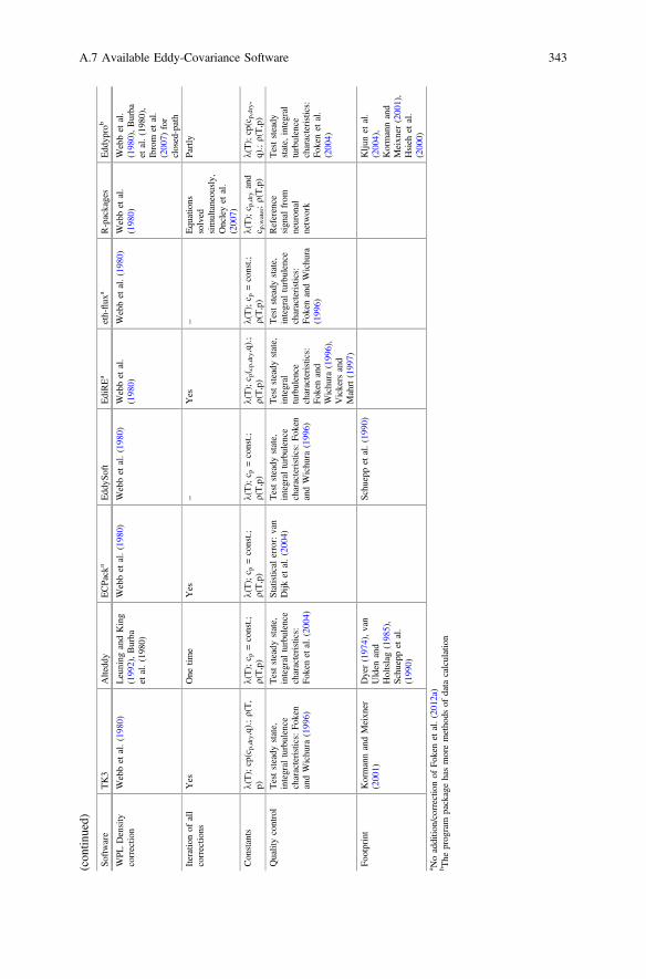
A.7 Available Eddy-Covariance Software

Overview of software packages used for eddy-covariance measurements (Mauderet al. 2008; Foken et al. 2012a, updated).

A.6 Meteorological Measurements Stations 341

Software

TK3

Alteddy

ECPack

aEddyS

oft

EdiREa

eth-flu

xaR-packages

Eddypro

b

University

ofBayreuth,

KIT

Garmisch-Partenkirchen

Alterra.

Wageningen

University

ofWageningen

Max-Planck-Institu

teJena

University

ofEdinburgh

SwissFederal

Institu

teof

TechnologyZurich

NCAR/EOL

LiCor

(Univ.

Tuscia)

Devices

CSA

T3,

USA

-1,HS,

R2,R3,ATI-K,NUW,

Young;6262,7000,

7200,7500,7700,

KH20,EC150,

EC

155,

ADCOP-2,

Aerodyn,Los

Gatos

R2,R3,WMPro,

HS,

CSA

T3,

USA

-1,Young,

ATI-K;

6262,7500,

7000,7200,

KH20,

TGA100A

,Los

Gatos

DLT100

R2,R3,CSA

T3

KDTR90/TR617500,

KH20,Lym

an-a

CSA

T3,USA

-1,R2,

R3,HS,Windm

aster,

Young;6262,7000,

7200,7500,ADC

OP-2

many

CSA

T3,R2,R3,HS;

6262,7000,7500,

FM-100,

Monito

rLabs,

Scintrex

LMA3,

Los

Gatos

FMA

andFG

GA,

AerodyneQCL

CSA

T3,

KH20,7000,

7500,EC

150

standard,other

sensorspossible

R2,R3,

WMPro;

CSA

T3,

USA

-1,

6262,7500,700s

7550

(7200/7700)

Datapreparation

Testp

lausibility,spikes;

blockaverage;

timelag

(const/auto)

Testplausibility,

spikes;block

average;

timelag

(const/auto)

Testplausibility,

spikes;detrending

(linear);tim

elag

(const.)

Testplausibility,

spikes;block

average,

optio

nal

detrending;tim

elag

(const/auto)

Testplausibility,

spikes;optio

nal

detrending

(linear/filter);

blockaverage;

Tim

elag

(const/auto)

Testplausibility,

spikes;block

average,

optio

nal

detrending;tim

elag

(const/auto)

Spikes;block

average;

time

lag

Test

plausibility,

spikes;block

average;

optio

nal

detrending

time

lag(const/auto,

moisture

dependent)

Coordinate

rotatio

nPlanar

fit/2

Drotatio

n;head-correction

2Drotatio

n/planar

fit

Planar

fit/2

D/3D

rotatio

nPlanar

fit/2

D/3D

rotatio

nPlanar

fit/2

D/3D

rotatio

n2D

/3D

rotatio

nPlanar

fit,2D

rotatio

nPlanar

fit/2

D/3D

rotatio

n,van

Dijk

etal.

( 2004);Nakai

etal.(2006);

Nakai

and

Shim

oyam

a(2012)

Buoyancy

flux!

sensible

heat

flux

Schotanuset

al.(1983),

Liu

etal.(2001)

Schotanuset

al.

(1983),Liu

etal.

(2001)

Schotanuset

al.

(1983)

Schotanuset

al.

(1983),Liu

etal.

(2001)

Schotanuset

al.

(1983),Liu

etal.

(2001)

–Schotanuset

al.

(1983)

vanDijk

etal.

(2004)

Oxygen

correctio

nfor

KH20

Tanneret

al.(1993)

Tanneret

al.

(1993),vanDijk

etal.(2003)

Tanneret

al.

(1993),van

Dijk

etal.

(2003)

––

–vanDijk

etal.

(2003)

–

Highfrequency

loss

correctio

nMoore

(1986)

Moore

(1986),

Leuning

andKing

(1992)

Moore

(1986)

Eugster

andSenn

(1995)

Moore

(1986),

Eugster

andSenn

(1995)

Eugster

andSenn

(1995)

Horstand

Lenschow

(2009))

Moncrieffet

al.,

(1997) (con

tinued)

342 A.7 Available Eddy-Covariance Software

(con

tinued)

Software

TK3

Alteddy

ECPack

aEddyS

oft

EdiREa

eth-flu

xaR-packages

Eddypro

b

WPL

Density

correctio

nWebbet

al.(1980)

Leuning

andKing

(1992),Burba

etal.(1980)

Webbet

al.(1980)

Webbet

al.(1980)

Webbet

al.

(1980)

Webbet

al.(1980)

Webbet

al.

(1980)

Webbet

al.

(1980),Burba

etal.(1980),

Ibrom

etal.

(2007)

for

closed-path

Iterationof

all

correctio

nsYes

One

time

Yes

–Yes

–Equations

solved

simultaneously,

Oncleyet

al.

(2007)

Partly

Constants

k(T);cp(c

p,dry,q).;q(T,

p)k(T);c p

=const.;

q(T,p)

k(T);c p

=const.;

q(T,p)

k(T);c p

=const.;

q(T,p)

k(T);c p( cp,dry,q).;

q(T,p)

k(T);c p

=const.;

q(T,p)

k(T);c p

,dryand

c p,water;q(T,p)

k(T);cp(c

p,dry,

q).;q(T,p)

Qualitycontrol

Teststeady

state,

integral

turbulence

characteristics:Fo

ken

andWichura

(1996)

Teststeady

state,

integral

turbulence

characteristics:

Fokenetal.(2004)

Statistical

error:van

Dijk

etal.(2004)

Teststeady

state,

integral

turbulence

characteristics:Fo

ken

andWichura

(1996)

Teststeady

state,

integral

turbulence

characteristics:

Fokenand

Wichura

(1996),

Vickers

and

Mahrt(1997)

Teststeady

state,

integral

turbulence

characteristics:

FokenandWichura

(1996)

Reference

signal

from

neuronal

network

Teststeady

state,

integral

turbulence

characteristics:

Fokenet

al.

(2004)

Footprint

KormannandMeixner

(2001)

Dyer(1974),van

Ulden

and

Holtslag(1985),

Schueppet

al.

(1990)

Schueppet

al.(1990)

Klju

net

al.

(2004),

Kormannand

Meixner

(2001),

Hsieh

etal.

(2000)

a Noadditio

n/correctio

nof

Fokenet

al.(2012a)

b The

program

packagehasmoremethods

ofdata

calculation

A.7 Available Eddy-Covariance Software 343

A.8 Glossary

Advection: Transport of properties of the air (momentum, temperature, water vapor,etc.) by the wind. As a rule, horizontal transport is understood. Because ofadvection, air properties change in both horizontal coordinates, and the conditionsare no longer homogeneous. Vertical advection is the vertical movement air due tomass continuity rather than buoyancy, i.e. convection.

Atmospheric window: Frequency range of electromagnetic waves, which passthrough the atmosphere down to the ground with little absorption. Within thisfrequency range, remote sensing methods of the surface properties can be applied.The most important atmospheric windows are in the visible range from 0.3 to 0.9lm, in the IR-range from 8 to 13 lm, and in the microwave range for wave lengthsgreater than 1 mm for surface wetness.

Bolometer: A device for measuring radiant energy by using thermally-sensitiveelectric sensors (thermocouple, thermistor, platinum wire).

Calm: State of the atmosphere with no discernible air motion. Thecalm-threshold is the threshold speed of cup anemometers, which is about 0.3 ms−1.A wind direction cannot be determined under these circumstances.

CET: Abbreviation of Central European Time. It is the mean local time at 15°longitudes, and differs from UTC by 1 hour.

Clausius-Clapeyron equation: Clapeyron 1834 established and Clausius 1850gave the reasons for the equations for the temperature dependence of equilibriumwater-vapour pressure at saturation. Because of the equation’s strong exponentialdependence on temperature, the amount of water vapour in the atmosphereincreases significantly with temperatures, and the atmosphere can therefore storemore latent heat at higher temperatures.

Climate element: Meteorological and other parameters that characterize (indi-vidually or in combinations) different climate types. These are state variables andfluxes.

Coherence: In generally, coherence is a constant phase relation between twowaves. Coherent structures in atmospheric turbulence research are velocity, tem-perature, and other structures, which are significantly larger and longer-lived thanthe smallest local eddies (e.g. squall lines, convective cells).

Coriolis force: Fictitious force in a rotating coordinate system, and named afterthe mathematician Coriolis (1792–1843). It is a force normal to the velocity vectorcausing a deflection to the right in the Northern hemisphere and to the left in theSouthern hemisphere.

Coriolis parameter: Twice the value of the angular velocity of the Earth for acertain location of the latitude u: f=2 X sin u. At the equator f = 0, on the Northernhemisphere positive and on the Southern hemisphere negative.

Dissipation: Conversion of kinetic energy by work against the viscous stresses.Under turbulent conditions, it is the conversion of the kinetic energy of the smallesteddies into heat.

344 A.8 Glossary

Element, meteorological: see climate elementEntrainment: Exchange process at the top of the atmospheric boundary layer,

and is due to the actions of eddies that are smaller than those in the mixed layer.Fetch: Windward distance from a measurements point to a change of the surface

properties or an obstacle; extent of a measurements field for micrometeorologicalresearch.

Froude number: Dimensionless ratio of the inertia force to the gravity forceFr=V2L−1g−1 where V is a characteristic velocity and L is a characteristic length.For flow over hills, L is the characteristic distance between hills or obstacles. Inthese cases, the external Froude number with the Brunt-Väisälä frequency N isused, see Eq. (3.35): Fr= V N−1L−1.

Gas constant: Proportionality factor of the equation of state for ideal gases, andis expressed in mol. In meteorology, the gas constant is expressed in mass units,and a special gas constant for dry air is used. In moist air, the temperature in theequation of state must be replaced by the virtual temperature (see below).

Gravity waves: Gravity waves are generated at the interface of two atmosphericlayers under stable stratification caused by buoyancy and gravity forces.

Hysteresis: The change between two states that depends on the way the changeoccurs, for example, the characteristics of a moisture sensor are different for wettingand drying.

Inversion: An air layer where the temperature increases with the altitude insteadof the usual decrease. Inversions are of two types; surface inversion due to long-wave radiation from the ground, and elevated or free inversions e.g. at the top of theatmospheric boundary layer.

Kelvin-Helmholtz instability: A dynamic instability caused by strong windshear resulting in breaking waves or billow clouds (Sc, Ac lent). Typically, theseoccur at inversions or above hills. They also can occur over obstacles and forests.

Leaf area density: The vertical probability density function of the leaf area.Leaf area index: Ratio of the leaf area (upper side) within a vertical cylinder to

the bottom area of the cylinder.Low-level jet: Vertical band of strong winds in the lower part of the atmospheric

boundary layer. For stable stratification, the low-level jet develops at the upperborder of the nocturnal surface inversion. Typical heights are 100–300 m, andsometimes lower.

LTST: Abbreviation for Local True Solar Time. It is the time related to themeridian of all points on the same longitude. The local true solar time is the solartime measured from the daily lower culmination of the sun and changes with thetime equation, which is the difference between the real and the mean solar time. Thetime equation is positive if the local true solar time earlier culminates than the meansolar time (sun day). It changes between –14 min 24 s (approx. middle of February)and +16 min 21 s (approx. beginning of November). For an approximation relationsee A4.

Matrix potential: A measure of the absorption and capillary forces of the solidsoil matrix on the soil water. Its absolute value is called tension.

A.8 Glossary 345

Mixed layer: A layer of strong vertical mixing due to convection resulting invertically-uniform values of potential temperature and wind speed but decreasingvalues of moisture. It is often capped by an inversion layer (see above).

MST: Abbreviation for Mean Solar Time. Time related to the meridian of thelocation and for all locations of the same longitude. The mean solar time is the solartime measured from the lower culmination of the sun. It is calculated by addition of 4minutes to the universal time (UT) for each degree of longitude in eastward direction.

Parameterization: Representation of complicated relations in models by moresimple combinations of parameters, which are often only valid under certaincircumstances.

Rossby similarity: In the free atmosphere, the Rossby number is the ratio of theinertial force to the Coriolis force. In the atmospheric boundary layer, the roughnessRossby number is the ratio of the friction velocity to the Coriolis parameter, Ro=u*/(f z0). The friction Rossby number is an assessment of the ageostrophic componentof the wind.

Stability of the stratification: The static stability separates turbulent and lam-inar flow conditions depending on the gradient of the potential temperature (seebelow). If the potential temperature decreases with height, then the stratification isunstable, but if it increases with height, then the stratification is stable. Due to theeffects of vertical wind sheer, the statically-stable range is turbulent up to the criticalRichardson number.

Temperature, potential: The temperature of a dry air parcel that is movedadiabatically to a pressure of 1000 hPa, see Eq. (2.22).

Temperature, virtual: The temperature of a dry air parcel if it had the samedensity as a moist air parcel. The virtual temperature is slightly higher than thetemperature of moist air, see Eq. (2.14).

Transmission: Permeability of the atmosphere for radiation. The radiation canbe reduced e.g. by gases, aerosols, particles, and water droplets.

UTC: Abbreviation for Universal Time Coordinated, a time scale based on theinternational atomic time by setting the zero point to the zero meridian (GreenwichMeridian), with the mean solar day as a basic unit. It is the basis for political andscientific time.

Wind, geostrophic: Wind above the atmospheric boundary layer where pressuregradient force and Coriolis force (see above) are in equilibrium.

A.9 Micrometeorological Standards Used in Germany

In Germany, Austria, and Switzerland meteorological measurements techniques andsome applied meteorological methods are standardized. Some of these standardswere incorporated in the international ISO standards. Because these standards areavailable in English, only the most important standards are given. The relevantstandards appear in volume 1B of the “VDI/DIN Handbook on Keeping the AirClean” (Queitsch 2002, update 2017):

346 A.8 Glossary

VDI/DIN Sheet Content

3781 2, 4 Atmospheric diffusion of pollutants

3782 1, 3, 5–7 Environmental meteorology—Atmospheric dispersionmodels

3783 1, 2, 4–6, 8–10, 12–14, 16, 18–21

Dispersion of pollutants in the atmosphere; dispersion ofemissions by accidental releases

3784 1, 2 Environmental meteorology; cooling towers

3785 1, 2 Urban climate, Mobile measurements systems

3786 1–9, 11–14, 16–18,20

Environmental meteorology—Meteorologicalmeasurements

3787 1, 2, 5, 9,10 Environmental meteorology—Climate and air pollution

3788 1 Environmental meteorology—Dispersion of odorants

3789 Environmental meteorology—Interactions betweenatmosphere and surfaces

3790 1–3 Environmental meteorology—Emissions of gases

3945 1, 3, 5 Environmental meteorology—Atmospheric dispersionmodels

4320 1–3 Measurement of atmospheric depositions

Because of a lack in the literature on meteorological measurements systems, theVDI/DIN 3786 (Sheets 1–20) and the relevant ISO standards may be of interest to awide readership:

VDI/DIN,ISO

Issued Title

ISO 16622 09/2002 Meteorology—Sonic anemometers/thermometers—Acceptance test methods for mean wind measurements

ISO17713-1

05/2007 Meteorology—Wind measurements—Part 1: Wind tunnel testmethods for rotating anemometer performance

ISO/DIS17714

07/2007 Meteorology—Air temperature measurements—Test methodsfor comparing the performance of thermometer shields/screensand defining important characteristics

ISO28902-1

01/2012 Air quality—Environmental meteorology—Part 1:Ground-based remote sensing of visual range by lidar

ISO/DIS28902-2

11/2016 Air quality—Environmental meteorology—Part 2:Ground-based remote sensing of wind by heterodyne pulsedDoppler lidar

VDI 3786Sheet 1

03/2013 Environmental meteorology—Meteorological measurementsFundamentals

VDI 3786Sheet 2

12/2000new: 2017

Environmental meteorology—Meteorological measurementsconcerning questions of air pollution—Wind

(continued)

A.9 Micrometeorological Standards Used in Germany 347

(continued)

VDI/DIN,ISO

Issued Title

VDI 3786Sheet 3

10/2012 Environmental meteorology—Meteorological measurements—Air temperature

VDI 3786Sheet 4

06/2013 Environmental meteorology—Meteorological measurements—Air humidity

VDI 3786Sheet 5

10/2015 Environmental meteorology—Meteorological measurements—Radiation

VDI 3786Sheet 6

10/1983new: 2017

Meteorological measurements of air pollution—turbidity ofground—level atmosphere standard visibility

VDI 3786Sheet 7

10/2012 Environmental meteorology—Meteorological measurements—Precipitation

VDI 3786Sheet 8

09/2015 Environmental meteorology—Meteorological measurements—Aerological measurements

VDI 3786Sheet 9

10/2007 Environmental Meteorology—Meteorological measurements—Visual weather observations

VDI 3786Sheet 10

Retracted

VDI 3786Sheet 11

07/2015 Environmental meteorology—Ground-based remote sensingof the wind vector and the vertical structure of the boundarylayer—Doppler sodar

VDI 3786Sheet 12

10/2008new: 2017

Environmental meteorology—Meteorological measurements—Turbulence measurements with sonic anemometers

VDI 3786Sheet 13

08/2006new: 2018

Environmental meteorology—Meteorological measurements—Measuring station

VDI 3786Sheet 14

12/2001 Environmental meteorology—Ground-based remote sensingof the wind vector—Doppler wind LIDAR

VDI 3786Sheet 15

Replaced by ISO 28902-1

VDI 3786Sheet 16

07/2010 Environmental meteorology—Meteorological measurements—Atmospheric pressure

VDI 3786Sheet 17

02/2007 Environmental meteorology—Ground-based remote sensingof the wind vector—Wind profiler radar

VDI 3786Sheet 18

05/2010 Environmental meteorology—Ground-based remote sensingof temperature—Radio-acoustic sounding systems (RASS)

VDI 3786Sheet 19

10/2016(draft)

Environmental meteorology - Ground-based remote sensing ofmeteorological parameters - Particle backscatter lidar

VDI 3786Sheet 20

09/2014 Environmental meteorology—Ground-based remote sensingof precipitation—Weather radar

348 A.9 Micrometeorological Standards Used in Germany

References

André J-C, Bougeault P and Goutorbe J-P (1990) Regional estimates of heat and evaporationfluxes over non-homogeneous terrain, Examples from the HAPEX-MOBILHY programme.Boundary-Layer Meteorol. 50:77–108.

Andreas EL (2002) Parametrizing scalar transfer over snow and ice: A review. J Hydrometeorol.3:417–432.

Beljaars ACM, Schotanus P and Nieuwstadt FTM (1983) Surface layer similarity undernonuniform fetch conditions. J Climate Appl Meteorol. 22:1800–1810.

Beljaars ACM and Holtslag AAM (1991) Flux parametrization over land surfaces for atmosphericmodels. J Appl Meteorol. 30:327–341.

Beyrich F, Herzog H-J and Neisser J (2002) The LITFASS project of DWD and the LITFASS-98Experiment: The project strategy and the experimental setup. Theor Appl Climat. 73:3–18.

Beyrich F and Mengelkamp H-T (2006) Evaporation over a heterogeneous land surface:EVA_GRIPS and the LITFASS-2003 experiment - an overview. Boundary-Layer Meteorol.121:5–32.

Bolle H-J, André J-C, Arrie JL, Barth HK, Bessemoulin P, A. B, DeBruin HAR, Cruces J,Dugdale G, Engman ET, Evans DL, Fantechi R, Fiedler F, Van de Griend A, Imeson AC,Jochum A, Kabat P, Kratsch P, Lagouarde J-P, Langer I, Llamas R, Lopes-Baeza E, MeliaMuralles J, Muniosguren LS, Nerry F, Noilhan J, Oliver HR, Roth R, Saatchi SS, SanchezDiaz J, De Santa Olalla M, Shutleworth WJ, Sogaard H, Stricker H, Thornes J, Vauclin M andWickland D (1993) EFEDA: European field experiment in a desertification-threatened area.Ann Geophys. 11:173–189.

Braam M, Moene A, Beyrich F and Holtslag AM (2014) Similarity relations for CT2 in the unstable

atmospheric surface layer: Dependence on regression approach, observation height andstability range. Boundary-Layer Meteorol. 153:63–87.

Businger JA, Miyake M, Inoue E, Mitsuta Y and Hanafusa T (1969) Sonic anemometercomparison and measurements in the atmospheric surface layer. J Meteor Soc Japan. 47:1–12.

Businger JA, Wyngaard JC, Izumi Y and Bradley EF (1971) Flux-profile relationships in theatmospheric surface layer. J Atmos Sci. 28:181–189.

Caughey SL and Readings CJ (1975) Turbulent fluctuations in convective conditions. Quart J RoyMeteorol Soc. 101:537–542.

Cohen ER and Taylor BN (1986) The 1986 adjustment of the fundamental physical constants.International Council of Scientific Unions (ICSU), Committee on Data for Science andTechnology (CODATA). CODATA-Bull. No. 63:36 pp.

Dyer AJ and Hicks BB (1970) Flux-gradient relationships in the constant flux layer. Quart J RoyMeteorol Soc. 96:715–721.

Dyer AJ (1974) A review of flux-profile-relationships. Boundary-Layer Meteorol. 7:363–372.

© Springer-Verlag Berlin Heidelberg 2017T. Foken, Micrometeorology, DOI 10.1007/978-3-642-25440-6

349

Dyer AJ, Garratt JR, Francey RJ, McIlroy IC, Bacon NE, Hyson P, Bradley EF, Denmead DT,Tsvang LR, Volkov JA, Kaprov BM, Elagina LG, Sahashi K, Monji N, Hanafusa T,Tsukamoto O, Frenzen P, Hicks BB, Wesely M, Miyake M and Shaw WJ (1982) Aninternational turbulence comparison experiment (ITCE 1976). Boundary-Layer Meteorol.24:181–209.

Dyer AJ and Bradley EF (1982) An alternative analysis of flux-gradient relationships at the 1976ITCE. Boundary-Layer Meteorol. 22:3–19.

Eugster W and Senn W (1995) A cospectral correction for measurement of turbulent NO2 flux.Boundary-Layer Meteorol. 74:321–340.

Fernando HJS, Pardyjak ER, Di Sabatino S, Chow FK, De Wekker SFJ, Hoch SW, Hacker J,Pace JC, Pratt T, Pu Z, Steenburgh WJ, Whiteman CD, Wang Y, Zajic D, Balsley B,Dimitrova R, Emmitt GD, Higgins CW, Hunt JCR, Knievel JC, Lawrence D, Liu Y,Nadeau DF, Kit E, Blomquist BW, Conry P, Coppersmith RS, Creegan E, Felton M,Grachev A, Gunawardena N, Hang C, Hocut CM, Huynh G, Jeglum ME, Jensen D,Kulandaivelu V, Lehner M, Leo LS, Liberzon D, Massey JD, McEnerney K, Pal S, Price T,Sghiatti M, Silver Z, Thompson M, Zhang H and Zsedrovits T (2015) The MATERHORN:Unraveling the intricacies of mountain weather. Bull Amer Meteorol Soc. 96:1945–1967.

Fischer G (ed) (1988) Landolt-Börnstein: Numerical Data and Functional Relationships in Scienceand Technology,Group V: Geophysics and space research, Volume 4: Meteorology,Subvolume b: Physical and chemical properties of the air. Springer, Berlin, Heidelberg,570 pp.

Foken T and Skeib G (1983) Profile measurements in the atmospheric near-surface layer and theuse of suitable universal functions for the determination of the turbulent energy exchange.Boundary-Layer Meteorol. 25:55–62.

Foken T and Kretschmer D (1990) Stability dependence of the temperature structure parameter.Boundary-Layer Meteorol. 53:185–189.

Foken T (1990) Turbulenter Energieaustausch zwischen Atmosphäre und Unterlage - Methoden,meßtechnische Realisierung sowie ihre Grenzen und Anwendungsmöglichkeiten. Ber DtWetterdienstes. 180:287 pp.

Foken T, Skeib G and Richter SH (1991) Dependence of the integral turbulence characteristics onthe stability of stratification and their use for Doppler-Sodar measurements. Z Meteorol.41:311–315.

Foken T (1996) Turbulenzexperiment zur Untersuchung stabiler Schichtungen. BerPolarforschung. 188:74–78.

Foken T and Wichura B (1996) Tools for quality assessment of surface-based flux measurements.Agrical Forest Meteorol. 78:83–105.

Foken T, Jegede OO, Weisensee U, Richter SH, Handorf D, Görsdorf U, Vogel G, Schubert U,Kirzel H-J and Thiermann V (1997) Results of the LINEX-96/2 Experiment. Dt Wetterdienst,Forsch. Entwicklung, Arbeitsergebnisse. 48:75 pp.

Foken T (1998) Ergebnisse des LINEX-97/1 Experimentes. Dt Wetterdienst, Forsch. Entwicklung,Arbeitsergebnisse. 53:38 pp.

Foken T, Göckede M, Mauder M, Mahrt L, Amiro BD and Munger JW (2004) Post-field dataquality control. In: Lee Xet al (eds.), Handbook of Micrometeorology: A Guide for SurfaceFlux Measurement and Analysis. Kluwer, Dordrecht, 181–208.

Foken T (2006) 50 years of the Monin-Obukhov similarity theory. Boundary-Layer Meteorol.119:431–447.

Foken T, Leuning R, Oncley SP, Mauder M and Aubinet M (2012a) Corrections and data qualityIn: Aubinet Met al (eds.), Eddy Covariance: A Practical Guide to Measurement and DataAnalysis. Springer, Dordrecht, Heidelberg, London, New York, 85–131.

Foken T, Meixner FX, Falge E, Zetzsch C, Serafimovich A, Bargsten A, Behrendt T, Biermann T,Breuninger C, Dix S, Gerken T, Hunner M, Lehmann-Pape L, Hens K, Jocher G,Kesselmeier J, Lüers J, Mayer JC, Moravek A, Plake D, Riederer M, Rütz F, Scheibe M,

350 References

Siebicke L, Sörgel M, Staudt K, Trebs I, Tsokankunku A, Welling M, Wolff V and Zhu Z(2012b) Coupling processes and exchange of energy and reactive and non-reactive trace gasesat a forest site – results of the EGER experiment. Atmos Chem Phys. 12:1923–1950.

Frenzen P and Vogel CA (2001) Further studies of atmospheric turbulence in layers near thesurface: Scaling the TKE budget above the roughness sublayer. Boundary-Layer Meteorol.99:173–458.

Garratt JR (1980) Surface influence upon vertical profiles in the atmospheric near surface layer.Quart J Roy Meteorol Soc. 106:803–819.

Garratt JR and Hicks BB (1990) Micrometeorological and PBL experiments in Australia.Boundary-Layer Meteorol. 50:11–32.

Gavrilov AS and Petrov JS (1981) Ocenka totschnosti opredelenija turbulentnych potokov postandartnym gidrometeorologitscheskim izmerenijam nad morem. Meteorol Gidrol:52–59.

Goldbach A and Kuttler W (2013) Quantification of turbulent heat fluxes for adaptation strategieswithin urban planning. Int J Climatol. 33:143–159.

Goutorbe JP, Lebel T, Tinga A, Bessemoulin P, Brouwer J, Dolman H, Engman ET, Gash JGC,Hoepffner M, Kabat P, Kerr YH, Monteny B, Prince SD, Said F, Sellers P and Wallace J(1994) HAPEX-SAHEL: A large scale study of land atmosphere interactions in the semi-aridtropics. Ann Geophys. 12:53–64.

Grimmond CSB, King TS, Cropley FD, Nowak DJ and Souch C (2002) Local-scale fluxes ofcarbon dioxide in urban environments: methodological challenges and results from Chicago.Environm Pollution. 116, Supplement 1:S243-S254.

Grimmond CSB, Salmond JA, Oke TR, Offerle B and Lemonsu A (2004) Flux and turbulencemeasurements at a densely built-up site in Marseille: Heat, mass (water and carbon dioxide),and momentum. J Geophys Res: Atmosph. 109:D24101.

Grimmond CSB (2006) Progress in measuring and observing the urban atmosphere. Theor ApplClimat. 84:3–22.

Handorf D, Foken T and Kottmeier C (1999) The stable atmospheric boundary layer over anAntarctic ice sheet. Boundary-Layer Meteorol. 91:165–186.

Hantel M (2013) Einführung Theoretische Meteorologie. Springer Spektrum, Berlin,Heidelberg,430 pp.

Hartmann DL (1994) Global Physical Climatology. Academic Press, San Diego, New York,408 pp.

Hartogensis OK and DeBruin HAR (2005) Monin-Obukhov similarity functions of the structureparameter of temperature and turbulent kinetic energy dissipation in the stable boundary layer.Boundary-Layer Meteorol. 116:253–276.

Hess GD, Hicks BB and Yamada T (1981) The impact of the Wangara experiment.Boundary-Layer Meteorol. 20:135–174.

Hicks BB (1981) An examination of the turbulence statistics in the surface boundary layer.Boundary-Layer Meteorol. 21:389–402.

Högström U (1988) Non-dimensional wind and temperature profiles in the atmospheric surfacelayer: A re-evaluation. Boundary-Layer Meteorol. 42:55–78.

Högström U (1990) Analysis of turbulence structure in the surface layer with a modified similarityformulation for near neutral conditions. J Atmos Sci. 47:1949–1972.

Horst TW, Kleissl J, Lenschow DH, Meneveau C, Moeng CH, Parlange MB, Sullivan PP andWeil JC (2004) HATS: Field observations to obtain spatially filtered turbulence fields fromcrosswind arrays of sonic anemometers in the atmospheric surface layer. J Atmos Sci.61:1566–1581.

Horst TW and Lenschow DH (2009) Attenuation of scalar fluxes measured withspatially-displaced sensors. Boundary-Layer Meteorol. 130:275–300.

Hsieh C-I, Katul G and Chi T-W (2000) An approximate analytical model for footprint estimationof scalar fluxes in thermally stratified atmospheric flows. Adv Water Res. 23:765–772.

Hughes DW, Yallop BD and Hohenkerk CY (1989) The equation of time. Monthly Notice RoyAstron Soc. 238:1529–1535.

References 351

Ibrom A, Dellwik E, Larsen SE and Pilegaard K (2007) On the use of the Webb–Pearman–Leuning theory for closed-path eddy correlation measurements. Tellus. B 59:937–946.

Izumi Y (1971) Kansas 1968 field program data report. Air Force Cambridge ResearchLaboratory, Bedford, MA, 79 pp.

Kaimal JC and Finnigan JJ (1994) Atmospheric Boundary Layer Flows: Their Structure andMeasurement. Oxford University Press, New York, NY, 289 pp.

King JC, Anderson PS, Smith MC and Mobbs SD (1996) The surface energy and mass balance atHalley, Antarctica during winter. J Geophys Res. 101(D14):19119–19128.

Klein P and Clark JV (2007) Flow variability in a North American downtown street canyon.J Appl Meteorol Climatol. 46:851–877.

Kljun N, Calanca P, Rotach M and Schmid HP (2004) A simple parameterization for flux footprintpredictions. Boundary-Layer Meteorol. 112:503–523.

Kopp G and Lean JL (2011) A new, lower value of total solar irradiance: Evidence and climatesignificance. Geophys Res Letters. 38:L01706.

Kormann R and Meixner FX (2001) An analytical footprint model for non-neutral stratification.Boundary-Layer Meteorol. 99:207–224.

Kotthaus S and Grimmond CSB (2012) Identification of micro-scale anthropogenic CO2, heat andmoisture sources – Processing eddy covariance fluxes for a dense urban environment. AtmosEnvironm. 57:301–316.

Lettau HH and Davidson B (eds) (1957) Exploring the Atmosphere's First Mile. Pergamon Press,London, New York, 376 pp.

Leuning R and King KM (1992) Comparison of eddy-covariance measurements of CO2 fluxes byopen- and closed-path CO2 analysers. Boundary-Layer Meteorol. 59:297–311.

Li D, Bou-Zeid E and De Bruin HR (2012) Monin–Obukhov similarity functions for the structureparameters of temperature and humidity. Boundary-Layer Meteorol. 145:45–67.

Liou KN (1992) Radiation and Cloud Processes in the Atmosphere. Oxford University Press,Oxford, 487 pp.

Liu H, Peters G and Foken T (2001) New equations for sonic temperature variance and buoyancyheat flux with an omnidirectional sonic anemometer. Boundary-Layer Meteorol. 100:459–468.

Lothon M, Lohou F, Pino D, Couvreux F, Pardyjak ER, Reuder J, Vilà-Guerau de Arellano J,Durand P, Hartogensis O, Legain D, Augustin P, Gioli B, Lenschow DH, Faloona I, Yagüe C,Alexander DC, Angevine WM, Bargain E, Barrié J, Bazile E, Bezombes Y, Blay-Carreras E,van de Boer A, Boichard JL, Bourdon A, Butet A, Campistron B, de Coster O, Cuxart J,Dabas A, Darbieu C, Deboudt K, Delbarre H, Derrien S, Flament P, Fourmentin M, Garai A,Gibert F, Graf A, Groebner J, Guichard F, Jiménez MA, Jonassen M, van den Kroonenberg A,Magliulo V, Martin S, Martinez D, Mastrorillo L, Moene AF, Molinos F, Moulin E,Pietersen HP, Piguet B, Pique E, Román-Cascón C, Rufin-Soler C, Saïd F, Sastre-Marugán M,Seity Y, Steeneveld GJ, Toscano P, Traullé O, Tzanos D, Wacker S, Wildmann N and Zaldei A(2014) The BLLAST field experiment: Boundary-Layer Late Afternoon and SunsetTurbulence. Atmos Chem Phys. 14:10931–10960.

Lumley JL and Panofsky HA (1964) The structure of atmospheric turbulence. IntersciencePublishers, New Yotk, 239 pp.

Maronga B (2013) Monin–Obukhov similarity functions for the structure parameters oftemperature and humidity in the unstable surface layer: Results from high-resolutionlarge-eddy simulations. J Atmos Sci. 71:716–733.

Mauder M, Foken T, Clement R, Elbers J, Eugster W, Grünwald T, Heusinkveld B and Kolle O(2008) Quality control of CarboEurope flux data - Part 2: Inter-comparison of eddy-covariancesoftware. Biogeoscience. 5:451–462.

McBean GA (1971) The variation of the statistics of wind, temperature and humidity fluctuationswith stability. Boundary-Layer Meteorol. 1:438–457.

McBean GA, Bernhardt K, Bodin S, Litynska Z, van Ulden AP and Wyngaard JC (1979) Theplanetary boundary layer. WMO, Note. 530:201 pp.

352 References

Mengelkamp H-T, Beyrich F, Heinemann G, Ament F, Bange J, Berger FH, Bösenberg J,Foken T, Hennemuth B, Heret C, Huneke S, Johnsen K-P, Kerschgens M, Kohsiek W, LepsJ-P, Liebethal C, Lohse H, Mauder M, Meijninger WML, Raasch S, Simmer C, Spieß T,Tittebrand A, Uhlenbrook S and Zittel P (2006) Evaporation over a heterogeneous landsurface: The EVA_GRIPS project. Bull Amer Meteorol Soc. 87:775–786.

Miyake M, Stewart RW, Burling RW, Tsvang LR, Kaprov BM and Kuznecov OA (1971)Comparison of acoustic instruments in an atmospheric flow over water. Boundary-LayerMeteorol. 2:228–245.

Moncrieff JB, Massheder JM, DeBruin H, Elbers J, Friborg T, Heusinkveld B, Kabat P, Scott S,Søgaard H and Verhoef A (1997) A system to measure surface fluxes of momentum, sensibleheat, water vapor and carbon dioxide. J Hydrol. 188–189:589–611.

Moore CJ (1986) Frequency response corrections for eddy correlation systems. Boundary-LayerMeteorol. 37:17–35.

Nakai T, van der Molen MK, Gash JHC and Kodama Y (2006) Correction of sonic anemometerangle of attack errors. Agrical Forest Meteorol. 136:19–30.

Nakai T and Shimoyama K (2012) Ultrasonic anemometer angle of attack errors under turbulentconditions. Agrical Forest Meteorol. 162–163:14–26.

Nelson MA, Pardyjak ER and Klein P (2011) Momentum and Turbulent Kinetic Energy BudgetsWithin the Park Avenue Street Canyon During the Joint Urban 2003 Field Campaign.Boundary-Layer Meteorol. 140:143–162.

Nemitz E, Hargreaves KJ, McDonald AG, Dorsey JR and Fowler D (2002) Micrometeorologicalmeasurements of the urban heat budget and CO2 emissions on a city scale. Environm SciTechn. 36:3139–3146.

Ohmura A, Steffen K, Blatter H, Greuell W, Rotach M, Stober M, Konzelmann T, Forrer J,Abe-Ouchi A, Steiger D and Neiderbäumer G (1992) Greenland Expedition, Progress ReportNo. 2, April 1991 to Oktober 1992. Swiss Federal Institute of Techology, Zürich, 94 pp.

Oncley SP, Foken T, Vogt R, Kohsiek W, DeBruin HAR, Bernhofer C, Christen A, van Gorsel E,Grantz D, Feigenwinter C, Lehner I, Liebethal C, Liu H, Mauder M, Pitacco A, Ribeiro L andWeidinger T (2007) The energy balance experiment EBEX-2000, Part I: Overview and energybalance. Boundary-Layer Meteorol. 123:1–28.

Panofsky HA, Tennekes H, Lenschow DH and Wyngaard JC (1977) The characteristics ofturbulent velocity components in the surface layer under convective conditions.Boundary-Layer Meteorol. 11:355–361.

Panofsky HA and Dutton JA (1984) Atmospheric Turbulence - Models and Methods forEngineering Applications. John Wiley and Sons, New York, 397 pp.

Patton EG,Horst TW, Sullivan PP, LenschowDH,Oncley SP, BrownWOJ,Burns SP,Guenther AB,HeldA,Karl T,Mayor SD, Rizzo LV, Spuler SM, Sun J, TurnipseedAA,Allwine EJ, Edburg SL,Lamb BK, Avissar R, Calhoun RJ, Kleissl J, Massman WJ, Paw U KT and Weil JC (2011) Thecanopy horizontal array turbulence study. Bull Amer Meteorol Soc. 92:593–611.

Poulos GS, Blumen W, Fritts DC, Lundquist JK, Sun J, Burns SP, Nappo C, Banta R, Newsom R,Cuxart J, Terradellas E, Balsley B and Jensen M (2002) CASES-99: A comprehensiveinvestigation of the stable nocturnal boundary layer. Bull Amer Meteorol Soc. 83:55–581.

Queitsch P (2002) TA Luft, Technische Anleitung zur Reinhaltung der Luft; SystematischeEinführung mit Text der TA Luft 2002. Bundesanzeiger-Verl.-Ges., Bonn, 180 pp.

Rotach M, Vogt R, Bernhofer C, Batchvarova E, Christen A, Clappier A, Feddersen B,Gryning SE, Martucci G, Mayer H, Mitev V, Oke TR, Parlow E, Richner H, Roth M, RouletY-A, Ruffieux D, Salmond JA, Schatzmann M and Voogt JA (2005) BUBBLE - an urbanboundary layer meteorology project. Theor Appl Climat. 81:231–261.

Salmond JA, Oke TR, Grimmond CSB, Roberts S and Offerle B (2005) Venting of heat andcarbon dioxide from urban canyons at night. J Appl Meteorol. 44:1180–1194.

Schotanus P, Nieuwstadt FTM and DeBruin HAR (1983) Temperature measurement with a sonicanemometer and its application to heat and moisture fluctuations. Boundary-Layer Meteorol.26:81–93.

References 353

Schuepp PH, Leclerc MY, MacPherson JI and Desjardins RL (1990) Footprint prediction of scalarfluxes from analytical solutions of the diffusion equation. Boundary-Layer Meteorol. 50:355–373.

Seiler W (1996) Results from the integrated research programme SANA, Phase I. Meteorol Z.5:179–278.

Sellers PJ, Hall FG, Asrar G, Strebel DE and Murphy RE (1988) The first ISLSCP fieldexperiment (FIFE). Bull Amer Meteorol Soc. 69:22–27.

Sellers PJ, Hall FG, Kelly RD, Black A, Baldocchi D, Berry J, Ryan M, Ranson KJ, Crill PM,Lettenmaier DP, Margolis H, Cihlar J, Newcomer J, Fitzjarrald D, Jarvis PG, Gower ST,Halliwell D, Williams D, Goodison B, Wickland DE and Guertin FE (1997) BOREAS in 1997:Experiment overview, scientific results, and future directions. J Geophys Res. 102:28 731–28769.

Skeib G (1980) Zur Definition universeller Funktionen für die Gradienten vonWindgeschwindigkeitund Temperatur in der bodennahen Luftschicht. Z Meteorol. 30:23–32.

SoegaardH andMøller-Jensen L (2003) Towards a spatial CO2 budget of ametropolitan region basedon textural image classification and flux measurements. Rem Sens Environm. 87:283–294.

Sonntag D (1989) Formeln verschiedenen Genauigkeitsgrades zur Berechnung der Sonnenkoordinaten.Abh Meteorol Dienstes DDR. 143:104 pp.

Sonntag D (1990) Important new values of the physical constants of 1986, vapour pressureformulations based on the ITC-90, and psychrometer formulae. Z Meteorol. 40:340–344.

Sorbjan Z (1986) Characteristics in the stable-continuous boundary layer. Boundary-LayerMeteorol. 35:257–275.

Sorbjan Z (1987) An examination of local similarity theory in the stably stratified boundary layer.Boundary-Layer Meteorol. 38:63–71.

Stull RB (1988) An Introduction to Boundary Layer Meteorology. Kluwer Acad. Publ., Dordrecht,Boston, London, 666 pp.

Swinbank WC (1964) The exponential wind profile. Quart J Roy Meteorol Soc. 90:119–135.Swinbank WC and Dyer AJ (1968) An experimental study on mircrometeorology. Quart J Roy

Meteorol Soc. 93:494–500.Swinbank WC (1968) A comparison between prediction of the dimensional analysis for the

constant-flux layer and observations in unstable conditions. Quart J Roy Meteorol Soc.94:460–467.

Tanner BD, Swiatek E and Greene JP (1993) Density fluctuations and use of the kryptonhygrometer in surface flux measurements. In: Allen RG (ed.), Management of Irrigation andDrainage Systems: Integrated Perspectives. American Society of Civil Engineers, New York,NY, 945–952.

Thiermann V and Grassl H (1992) The measurement of turbulent surface layer fluxes by use ofbichromatic scintillation. Boundary-Layer Meteorol. 58:367–391.

Thomas C and Foken T (2002) Re-evaluation of integral turbulence characteristics and theirparameterisations. 15th Conference on Turbulence and Boundary Layers, Wageningen, NL,15–19 July 2002 2002. Am. Meteorol. Soc., pp. 129–132.

Thomas C and Foken T (2007) Organised motion in a tall spruce canopy: Temporal scales,structure spacing and terrain effects. Boundary-Layer Meteorol. 122:123–147.

Tschalikov DV (1968) O profilja vetra i temperatury v prizemnom sloe atmosfery pri ustojtschivojstratifikacii (About the wind and temperature profile in the surface layer for stablestratification). Trudy GGO. 207:170–173.

Tsvang LR, Kaprov BM, Zubkovskij SL, Dyer AJ, Hicks BB, Miyake M, Stewart RW andMcDonald JW (1973) Comparison of turbulence measurements by different instuments;Tsimlyansk field experiment 1970. Boundary-Layer Meteorol. 3:499–521.

354 References

Tsvang LR, Zubkovskij SL, Kader BA, Kallistratova MA, Foken T, Gerstmann W, Przandka Z,Pretel J, Zelený J and Keder J (1985) International turbulence comparison experiment(ITCE-81). Boundary-Layer Meteorol. 31:325–348.

Tsvang LR, Fedorov MM, Kader BA, Zubkovskii SL, Foken T, Richter SH and Zelený J (1991)Turbulent exchange over a surface with chessboard-type inhomogeneities. Boundary-LayerMeteorol. 55:141–160.

Uttal T, Curry JA, Mcphee MG, Perovich DK, Moritz RE, Maslanik JA, Guest PS, Stern HL,Moore JA, Turenne R, Heiberg A, Serreze MC, Wylie DP, Persson OG, Paulson CA, Halle C,Morison JH, Wheeler PA, Makshtas A, Welch H, Shupe MD, Intrieri JM, Stamnes K,Lindsey RW, Pinkel R, Pegau WS, Stanton TP and Grenfeld TC (2002) Surface heat budget ofthe Arctic ocean. Bull Amer Meteorol Soc. 83:255–275.

van Dijk A, Kohsiek W and DeBruin HAR (2003) Oxygen sensitivity of krypton and Lyman-alphahygrometers. J Atm Oceanic Techn. 20:143–151.

van Dijk A, Kohsiek W and DeBruin HAR (2004) The principles of surface flux physics: theory,practice and description of the ECPACK library. University of Wageningen, Wageningen, 98pp.

van Ulden AP and Holtslag AAM (1985) Estimation of atmospheric boundary layer parameters fordiffusion applications. J Climate Appl Meteorol. 24:1196–1207.

VDI (2006) Umweltmeteorologie - Meteorologische Messungen - Messstation, VDI 3786, Blatt13. Beuth-Verlag, Berlin, 44 pp.

VDI (2015) Umweltmeteorologie: Wechselwirkungen zwischen Atmosphäre und Oberflächen,Berechnung der spektralen kurz- und der langwelligen Strahlung, VDI 3789 (Draft).Beuth-Verlag, Berlin, 95 pp.

Vesala T, Järvi L, Launiainen S, Sogachev A, Rannik Ü, Mammarella I, Siivola E, Keronen P,Rinne J, Riikonen ANU and Nikinmaa E (2008) Surface–atmosphere interactions overcomplex urban terrain in Helsinki, Finland. Tellus B. 60:188–199.

Vickers D and Mahrt L (1997) Quality control and flux sampling problems for tower and aircraftdata. J Atm Oceanic Techn. 14:512–526.

Vogt R, Christen A, Rotach MW, Roth M and Satyanarayana ANV (2006) Temporal dynamics ofCO2 fluxes and profiles over a Central European city. Theor Appl Climat. 84:117–126.

Wagner W and Pruß A (2002) The IAPWS Formulation 1995 for the Thermodynamic Propertiesof Ordinary Water Substance for General and Scientific Use. Journal of Physical and ChemicalReference Data. 31:387–535.

Webb EK (1970) Profile relationships: the log-linear range, and extension to strong stability.Quart J Roy Meteorol Soc. 96:67–90.

Webb EK, Pearman GI and Leuning R (1980) Correction of the flux measurements for densityeffects due to heat and water vapour transfer. Quart J Roy Meteorol Soc. 106:85–100.

Wulfmeyer V, Behrendt A, Kottmeier C, Corsmeier U, Barthlott C, Craig G, Hagen M,Althausen D, Aoshima F, Arpagaus M, Bauer HS, Bennett L, Blyth A, Brandau C,Champollion C, Crewell S, Dick G, Di Girolamo P, Dorninger M, Dufournet Y, Eigenmann R,Engelmann R, Flamant C, Foken T, Gorgas T, Grzeschik M, Handwerker J, Hauck C, HöllerH, Junkermann W, Kalthoff N, Kiemle C, Klink S, König M, Krauß L, Long CN, Madonna F,Mobbs S, Neininger B, Pal S, Peters G, Pigeon G, Richard E, Rotach M, Russchenberg H,Schwitalla T, Smith V, Steinacker R, Trentmann J, Turner DD, van Baelen J, Vogt S,Volkert H, T. W, Wernli H, Wieser A and Wirth M (2011) The convective and orographicallyinduced precipitation study (COPS): The scientific strategy, the field phase, and researchhighlights. Quart J Roy Meteorol Soc. 137:3–30.

Wyngaard JC, Izumi Y and Collins SA (1971) Behavior of the refractive-index-structure parameternear the ground. J Opt Soc Am. 61:1646–1650.

Wyngaard JC and Coté OR (1971) The budgets of turbulent kinetic energy and temperaturevariance in the atmospheric surface layer. J Atmos Sci. 28:190–201.

References 355

Wyngaard JC (1973) On surface layer turbulence. In: Haugen DH (ed.), Workshop onMicrometeorology. Am. Meteorol. Soc., Boston, 101–149.

Yaglom AM (1977) Comments on wind and temperature flux-profile relationships.Boundary-Layer Meteorol. 11:89–102.

Zilitinkevich SS and Tschalikov DV (1968) Opredelenie universalnych profilej skorosti vetra itemperatury v prizemnom sloe atmosfery (Determination of universal profiles of wind velocityand temperature in the surface layer of the atmosphere). Izv AN SSSR, Fiz Atm Okeana.4:294–302.

356 References

Index

AAbsorption coefficient, 273Advection, 122, 174, 344Ageostrophic method, 36Air pollution, 315Aktinometer, 257Albedo, 13Albedometer, 257Analogue to digital converter, 246Anemometer

cup, 260hot wire, 260laser, 260propeller, 260sonic, 260, 266

Ångström’s equation, 17Area averaging, 231Assmann’s aspiration psychrometer, 268Astronomical quantities, 332Austausch coefficient, 25

BBasic Surface Radiation Network, 258Bias, 291Biometeorology

human, 322Blending height, 99, 233Bolometer, 344Boundary layer

atmospheric, 7, 73internal, 91laminar, 8, 217molecular, 8, 217planetary, 7stable, 7thermal internal, 98

Boussinesq-approximation, 35Bowen ratio, 62Bowen-ratio method, 146

modified, 149Bowen-ratio similarity, 62, 120Bragg condition, 278Brunt-Väisälä frequency, 126, 230Buckingham’s P-theorem, 54Bulk approach, 40, 144Buoyancy, 38Buoyancy flux, 170Burba correction, 174Burst, 111

CCalm, 344Ceilometer, 279Change of the surface roughness, 309Changes of the albedo, 310Charnock approach, 50, 229Class-A-pan, 285Clausius-Clapeyron‘s equation, 209, 344Climate

local, 299Climate of hollow, 302Closure techniques, 40Cloud

genera, 16Coefficient

drag, 75Coherence, 344Cold-air flow, 306Comparability, 291Concentration distribution, 318Conditional sampling, 182Conductivity

thermal molecular, 18Constant flux layer, 8Constants, 330Convection

free, 76, 100Coordinate rotation, 165

© Springer-Verlag Berlin Heidelberg 2017T. Foken, Micrometeorology, DOI 10.1007/978-3-642-25440-6

357

Coriolis force, 37, 344Coriolis parameter, 64, 344Correction

angle of attack, 173buoyancy flux, 170density, 171flow distortion, 172precipitation, 275SND-, 170specific heat, 174spectral, 168transducer, 172WPL-, 171WPL-,modification, 173

Cosine response, 262Counter gradient, 111Coupling

atmosphere and plant canopies, 120model, 236

DDalton approach, 208Dalton number, 144Damköhler number

Kolmogorov-, 193turbulent, 193

Data collection, 245Deardorff velocity, 44, 76, 229Decibel, 247Declination, 333Decoupling, 99, 111, 118, 121Degradation, 311Deposition

dry, 189moist, 189wet, 189

Dewfall, 25Dew point, 49Diffusion coefficient

turbulent, 24, 40, 46, 211Diffusivity

molecular thermal, 18Displacement height. See zero-plane

displacementDissipation, 23, 344Distance constant, 252DNS. See simulation

direct numericalDrag coefficient, 144Dyer-Businger-Pandolfo-relationship, 57

EEcoclimate, 299

Eddyturbulent. See turbulence element

Eddy-accumulation method, 182hyperbolic relaxed, 185modified relaxed, 184relaxed, 184

Eddy-correlation method, 159, 181Eddy-covariance method, 4, 35, 39, 125, 159

basics, 161disjunct, 187generalized, 160

Eddy-covariance software, 341Einstein’s summation notation, 34Ejection, 111Ekman layer, 8Element

climate, 301, 344meteorological, 254, 344

Energyturbulent kinetic, 43

Energy balanceclosure, 127

Energy dissipation, 21, 45, 65, 72, 230dimensionless, 69

Energy spectrum, 68Enhanced vegetation index (EVI), 285Enhancement factor, 119Entrainment, 7, 345Entrainment parameter, 225Equation

barometric, 48turbulent energy, 43

Equation of motion, 33turbulent, 34

Errordynamic, 253radiation, 270wind, 275

Etalon, 258Eulerian length scale, 66Euler number, 37European wind atlas, 319Evaporation, 10, 26

actual, 212FAO reference, 214potential, 208

Evaporation equivalent, 48Evaporation measurements, 285Evaporimeter, 285Evapotranspiration, 26, 310Exchange

turbulent, 21Experiment, 338

358 Index

FF-correction, 259Fetch, 345Fick’s diffusion law, 318Flux

aggregation, 232density, 11turbulent, 46, 128

Flux-gradient similarity, 46Flux-variance relation, 181Flux-variance similarity, 63Footprint, 103, 159

climatology, 107dimension, 104model, 318

Force-restore method, 20Forest, 114Forest climate, 302Fourier transformation, 68Frequency

normalized, 24Friction velocity, 46Frost risk, 306Froude number, 229, 345Function

autocorrelation, 71universal, 56, 334

GGap

ecological, 5technical sensing, 7

Gap filling, 178Garden climate, 302Gas constant, 345Ground heat flux, 10, 18Ground heat storage, 18Ground water, 26Gust, 111Gustiness component, 229

HHaar wavelet, 176Heat capacity

volumetric, 18, 282Heat flux

latent, 10, 46sensible, 10, 46

Heightmixed-layer, 73

Holtslag-van Ulden approach, 215Humidity

absolute, 49measurements, 267

relative, 49scale, 53specific, 49units, 49

Hydrometeorology, 26Hygrometer

capacity, 267dew point, 267IR-, 163, 267UV-, 163, 267

Hysteresis, 345

IICOS, 191Inertia force

molecular, 37Inflection point, 111Interception, 26Intercomparison, 290Intermittency, 125Inversion, 345

capping, 7IR-thermometer, 257Isotropy

local, 66

KK-approach, 40Kelvin-Helmholtz instability, 120, 345Klimamichel, 322Kolmogorov constant, 67Kolmogorov’s microscale, 23, 65, 230

LLake climate, 302Lambert-Beer’s law, 273Land-sea wind circulation, 304Land use change, 307Laplace equation, 320Laplace transformation, 251Large-eddy simulation, 230Layer

mixed, 7, 9, 73, 118new equilibrium, 92

Leaf-area index, 87, 91, 213, 284, 345Length scale

turbulent, 65Lidar, 278Lloyd-Taylor function, 178Logger, 246Louis approach, 228Low-level-jet, 345Low pass filter, 246, 248Lupolen dome, 257

Index 359

Lysimeter, 285

MMacro-turbulence, 5MAD, 164, 178Magnus’s equation, 49Matrix potential, 345Measurement

microclimatological, 311Measurement planning, 287Measuring station

meteorological, 255, 340Meso-turbulence, 5Meteorology, 1

applied, 2environmental, 2

Michaelis-Menton function, 178Micro-front, 124Micrometeorology, 2

history, 2Mixed layer, 346Mixing length, 42Mixing ratio, 49Model, 207

big leaf, 219large scale, 227LES, 230multilayer, 216spectra, 70SVAT, 219

Momentum flux, 46Monin-Obukhov’s similarity theory, 54Mosaic approach, 234Mountain-valley-circulation, 304Multiplexer, 246

NNavier-Stokes equation, 33, 230, 306NDVI, 284NEON, 191Net radiometer, 257Noise, 247Nusselt number, 269Nyquist frequency, 248

OOasis effect, 25Obstacle, 101, 319Obukhov-Corrsin constant, 72Obukhov length, 55, 60Obukhov number, 55Ogive, 169O’KEYPS function, 57

Oversampling, 246Overspeeding, 261

PParameter

stability, 75aggregation, 232

Parametrization, 346Parameterization method, 151Penman approach, 210Penman-Monteith approach, 212Philip correction, 281Planar-fit method, 167Poisson equation, 38Power- law, 157Power spectrum, 68Prandtl layer, 8Prandtl number, 46, 222

turbulent, 46, 72Precipitation, 26Precipitation measurements, 275Precision, 291Predicted mean vote, 322Priestley-Tayler approach, 209Profile

in plant canopies, 89Profile equation, 221

neutral stratification, 46Profile method, 143, 154Propagation

sound, 320Psychrometer, 268Pyranometer, 257Pyrgeometer, 257Pyrheliometer, 257

QQuality assurance, 286

Eddy-covariance method, 174profile method, 152

Quality control, 288

RRadar, 278Radiation, 10

climate, 301direct sun, 257extraterrestrial, 333global, 13heat, 13longwave, 10, 13, 257measurements, 256PAR, 257, 284

360 Index

shield, 268shortwave, 10, 13, 257sun, 13

Radiometer, 257Radiosonde, 73Radix layer, 158Rain gauge, 275RASS, 278Regression

orthogonal, 291Residual layer, 7Resistance

approach, 219canopy, 220law, 75

Reynolds’s decomposition, 35Reynolds number, 37

roughness, 85, 224Reynolds’s postulate, 35Richardson number, 38, 59

bulk, 59, 74, 228critical, 60flux, 59gradient, 59

Rossby number, 37, 75Rossby similarity, 64, 75, 346Roughness, 83Roughness height. See roughness lengthRoughness length, 50

effective, 84for humidity, 51for scalars, 52for temperature, 51

Roughness parameter. See roughness lengthRoughness sublayer, 118Runoff, 26

SSample and hold circuit, 246Sampling

frequency, 248theorem, 247

Sand roughnessequivalent, 85

Scaleaerodynamic, 53atmospheric, 5climatological, 299geometric, 53

Schmidt number, 47turbulent, 47

Scintillometer, 279Sea smoke, 307

Shear stress, 46Similarity

scalar, 116Simulation

direct numerical, 231SI-units, 329Smagorinsky-Lilly parametrization, 231Sodar, 277Soil chamber measurements, 283Soil heat flux plate, 281Soil-vegetation-atmosphere-transfer model,

219Sound speed, 264Source-weight function, 104Spikes, 164Sprung’s psychrometric equation, 273Standards

German, 346Stanton number, 144Stefan-Boltzmann law, 15Stomata resistance, 213Stratification, 58, 346

stable, 125Stratification class

Klug-Manier, 316Pasquill, 316

Structurecoherent, 111constant, 71function, 71organized turbulent, 129ramp, 114

Structure function parameter, 72refraction, 72, 279temperature, 72, 279

Sublayerdynamical, 9roughness, 9

Sublayer-Stanton number, 222Sub-range

inertial, 23, 67Sunshine autograph according to

Campbell-Stokes, 17Surface

heterogeneous, 91Surface layer

atmospheric, 2Surface renewal method, 188Sweep, 111

TTDR-method, 281Temperature

Index 361

dimensionless, 217friction, 53measurements, 267physiological equivalent, 322potential, 346scale, 53sonic, 170, 265virtual, 170, 265, 346

Tensiometer, 280Tetens’ equation, 49Thermistor, 272Thermometer

bimetal, 267mercury, 267

Thethersonde, 253Tile approach, 234Tilt

correction, 165Time

Central European, 344mean local, 346real local, 345universal coordinated, 346

Time constant, 252, 268TKE-equation, 43

dimensionless, 68Topoclimate, 299Transfer function, 249, 260Transilient theory, 42Transmission, 346Transpiration, 26Turbulence

atmospheric, 22element, 3, 21frozen, 23spectrum, 22, 65

Turbulence characteristicintegral, 63, 76, 337

Turc approach, 208

Uu*-criterion, 179Universal Thermal Climate Index, 323Upper layer, 8Urban climate, 303Urban heat island, 303

VVegetation

high, 109index, 284

Velocityconvective, 44deposition, 191dimensionless, 217threshold, 261transfer, 192

Ventilation term, 213Von-Kármán constant, 58, 59

WWater balance equation, 26Water cycle, 26Wavelet analysis, 115Wind

energy use, 318geostrophic, 7, 36, 74, 346katabatic, 304measurements, 260power, 101

Windowatmospheric, 344

Wireresistance, 270thin platinum, 270

WPL correction, 171

ZZero-plane displacement, 53, 88Z-less scaling, 57, 125

362 Index