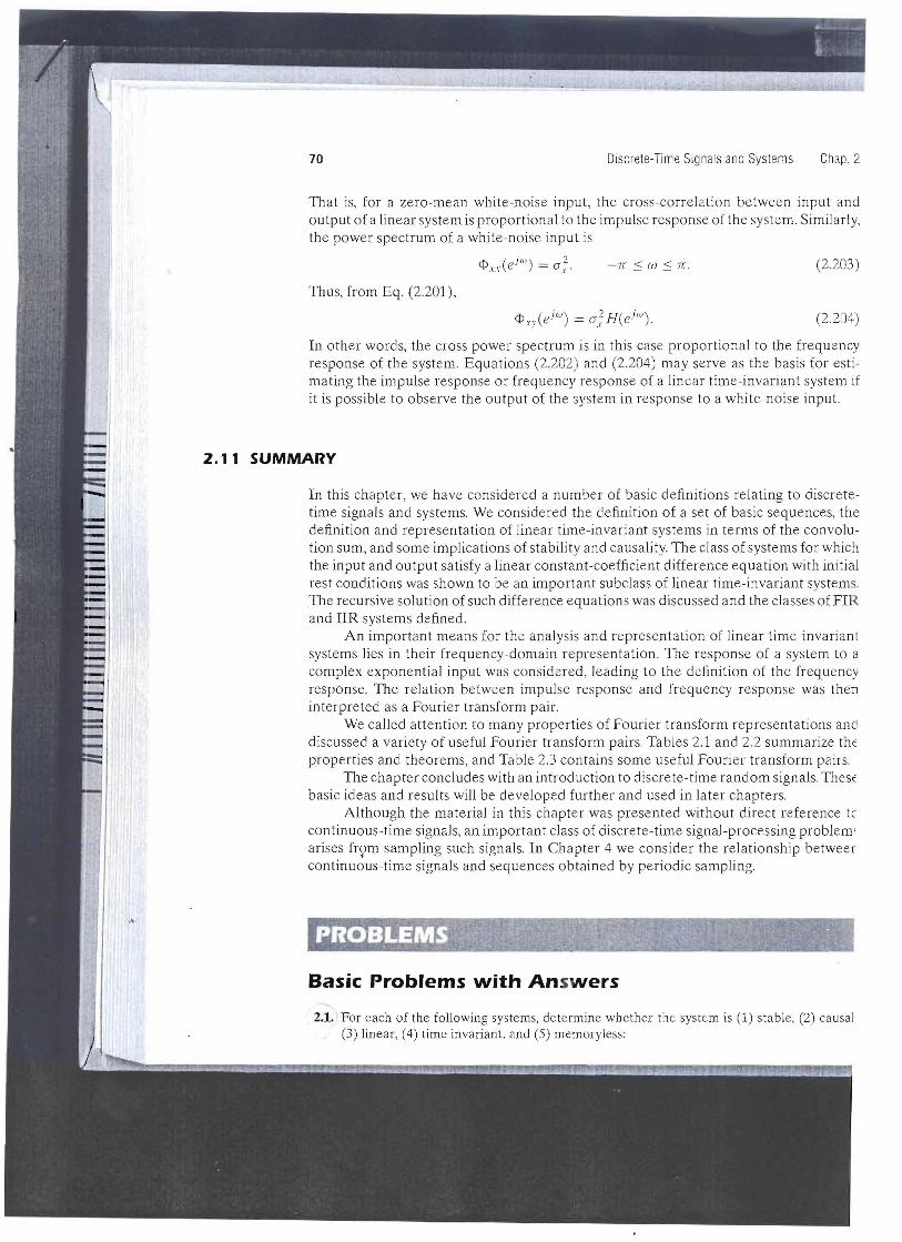
Discrete-Time Signals and Systems Chap. 270

That is, for a zero-mean white-noise input, the cross-correlation between input and output of a linear system is proportional to the impulse response of the system. Similarly, the power spectrum of a whi te-noise input is

'" ( iw) 2"'xx e = cJx ' -Jr .:::: W .:::: Jr. (2.203)

Thus, from Eq. (2.201),

(2.204)

In other words, the cross power spectrum is in this case proportional to the frequency response of the system. Equations (2.202) and (2.204) may serve as the bas is for esti­mating the impulse response or frequency response of a linear time-invariant system if it is possible to observe the output of the system in response to a white-noise input.

2.11 SUMMARY

In this chapter, we have considered a number of basic definitions re la ting to di screte­time signals and systems. We considered the definition of a set of basic sequences, the definition and representation of linear time-invariant systems in te rms of the convolu­tion sum, and some implica tions of stability and causality. The class of systems for which the input and output satisfy a linear constant-coefficient difference equation with initial rest conditions was shown to be an important subclass of linear time-invariant system. The recursive solution of such difference equations was discussed and the cla sses of FIR and IIR systems defined .

An importan t means for the analysis and representa tion of linear time-invariant systems lies in their frequency-domain representation. The response of a system to a complex exponential input was considered , leading to the definition of the frequ ency response. The relation betwee n impulse response and frequency response was then interpreted as a Fourier transform pair.

We called attention to many properties of Fourier transform representations and discussed a variety of useful Fourier transform pairs. Tables 2.1 and 2.2 summarize the properties and theorems, and Table 2.3 contains some useful Fourier transform pairs.

The chapter concludes with an introduction to discrete- time random signals. TheSe basic ideas and results will be developed further and used in later chapters.

Although the material in this chapter was presented without direc t reference tc continuous-time signals, an important class of discrete-time signal-processing problem~ arises fr9m sampling such signals. In Chapter 4 we consider the relationship betweer continuous-time signals and sequences obtained by periodic sampling.

Basic Problems with Answers

2.1. For each of the following systems, dete rmine whether the system is (1) stable, (2) causa l (3) linear, (4) time invariant. and (5) memoryless:

paz

Chap. 2 Problems 7 1

It and lilarly.

2.203)

2.204)

:juency Jr esti­stem if put.

liscrete­,Ices, the .onvolu­)r which th initial systems. :s ofFlR 1

nvariant tem to a 'equency was then

tions and la rize the m pairs. also These

:erence to problems

) between

~, (2) causal,

(a) T(x[nJ) =

(b) T(x [nJ) =

(c) T(x[nJ) =

(d) T(x[nl) =

(e) T(x[n]) = (f) T(x[n]) = (g) T(x[nJ) = (h) T(x[nJ) =

g[n]x[n] with g[n] given

,£Z=I1() x[k]

'£~:~~I1() x[k] x[n - no] exl111

ax[n] + b x[-n] x[n] + 3u[n + 1]

2.2. (a) The impulse response l1[n] of a linear time-invariant system is known to be zero, exce pt in the interva l No S n S N j • The input x[n] is known to be zero, except in the interval N2 S n S N3. As a result , the output is co nstrained to be zero, except in some interval N4 S n S Ns· Determine N4 and Ns in terms of No, Nt, N2, and N3·

(b) Ifx[n] is zero, except for N consecutive points, and h[n] is zero, except for M co nsecutive poin ts, what is the maximum number of consecutive points for which Y[I'l] can be nonzero?

2.3. By di rect evaluation of the convolution su m, de.te rmine the step response of a linear time­invariant system whose impulse response is

O<a<1.

2.4. Consider the linear co nstant-coefficie nt di ffere nce equation

y[n]- ~y [n - 1] + ~y[n - 2] = 2x[n - 1].

Determin e y[n] for n ::: 0 when x[l1] = o[n] and y[n] = 0, n < O.

2.5. A causal linear time-invariant system is described by the difference equation

Y[I1] - 5y[n - 1] + 6y [n - 2] = 2x [n - 1].

(a) D etermine the homogeneous response of the system, i. e., the possible outputs if x[n] = ofor all n. .

(b) Determine the impulse response of the system. (c) Determine th e step response of the syste m.

2.6. (a) Find the frequency response H(e iw ) of the linear time-invariant system whose inpu t a nd output satisfy the difference equa tion

y[n]- ~y[n - 1] = x[n] + 2x[n - 1] + x[n - 2].

(b) Write a di fference equation that characterizes a system whose frequency response is

. 1- Ie-ii" + e- i3(v

H(e l '") = 2 . 1 + le- iw + 2e- i2w

2 4

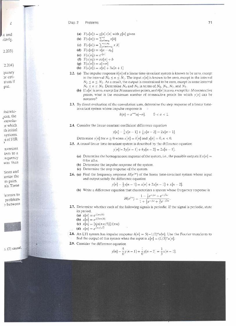
2.7. Determine whether each of the following signals is per iodic. If the signal is periodic, state its period. (a) x[n] = ei (lfl1 /6 )

(b) x[nJ = ei(3rr l1 / 4)

(c) x[nJ = [sin(7rn/5)] / (7rn) (d) x[n] = e/1r I1

/ h

2.8. An LTI sys tem has impulse response h[n] = 5(-1 / 2)" u ln J. Use the Fourier transform to find the output of this syste m when the input is x[n] = (1/3)"u[n].

2.9. Consider the difference equation

5 1 1 y[n] - 6y[n -1] + 6y[n - 2] = 3'x[n - 1].

75 Chap. 2 Problem s

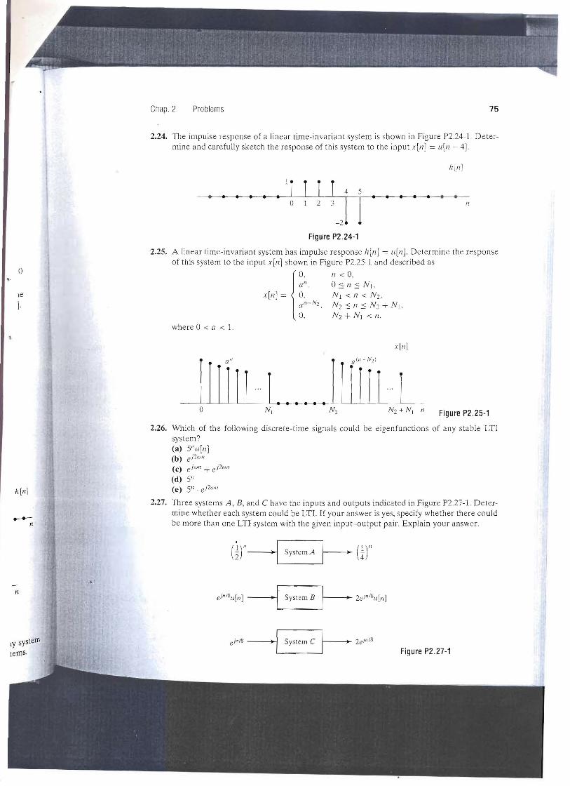
2.24. The impulse response of a li near time-invariant system is shown in Figure P2 .24-1. De ter­mine and carefully sketch the response of thi s system to the input x[n] = u[n - 4] .

h [n)

•1I I I I 4• • • • 5 • • • • • • o n

Figure P2 .24-1

2.25. A linear time-invariant system has impulse response h[n] = urn]. Determine the response of this system to the input x[nl shown in Figure P2.25 J an d described as

o 0, n < 0, an 0::: n::: N "

x[n] = 0, N) < n < N2. { a"- N2 . N 2::: n ::: N2 + N l ,\.

O. N2 + N J < n. where 0 < a < 1.

x[tI)

111lI l l • • • • • • 11 nTI 1 o Figure P2.25-1

2.26. Which of the following discrete-time signals could be eigenfunctio ns of any stable LTI system? (a) 5"I/[n1

ei2wI1(b) iwn + ei2w"(c) e

(d) 5" ei2wII(e) 5" ·h[nJ

2.27. Three systems A, E, and C ha ve the inputs and o utputs indicated in Figure P2.27-1. D eter­

--­ mine whether each system could be LTL If your answer is yes, specify whether the re could n be more than one LTI system with the gi ven input-o utput pair. Explain your answer.

. ·1 System A(~)"--+-I I

.,. n

·1' System B f-----'.~ 2eJnJ~u [nJ

ly systeJ1l eillJ8 ---+1 System C

terns. ·1 Figure P2.27-1

r 80 Discrete-Time Signals and Systems Chap 2

(c) Assume that the difference equation (property 1) remains the same, but the value y[o] is specified to be zero. Does this change your answer to either Part (a) or Part (b) ?

2.40. Consider the linear time-invariant sys tem with impulse response

h[n] = U)" urn]. where j = J=!.

Determine the steady-state response, i.e. , the response for large n , to the excitation

x[n] = cos(nn)u[nJ.

2.41. A linear time-invariant system has frequency response

2n (3)Iwl < 16 :2 '

2n (3)- - < Iwl < n.16 2 - ­

The input to the system is a periodic unit-impulse train with period N = 16; i.e ..

x[n] = L00

8[n + 16k]. k = - 'X)

Find the output of the system.

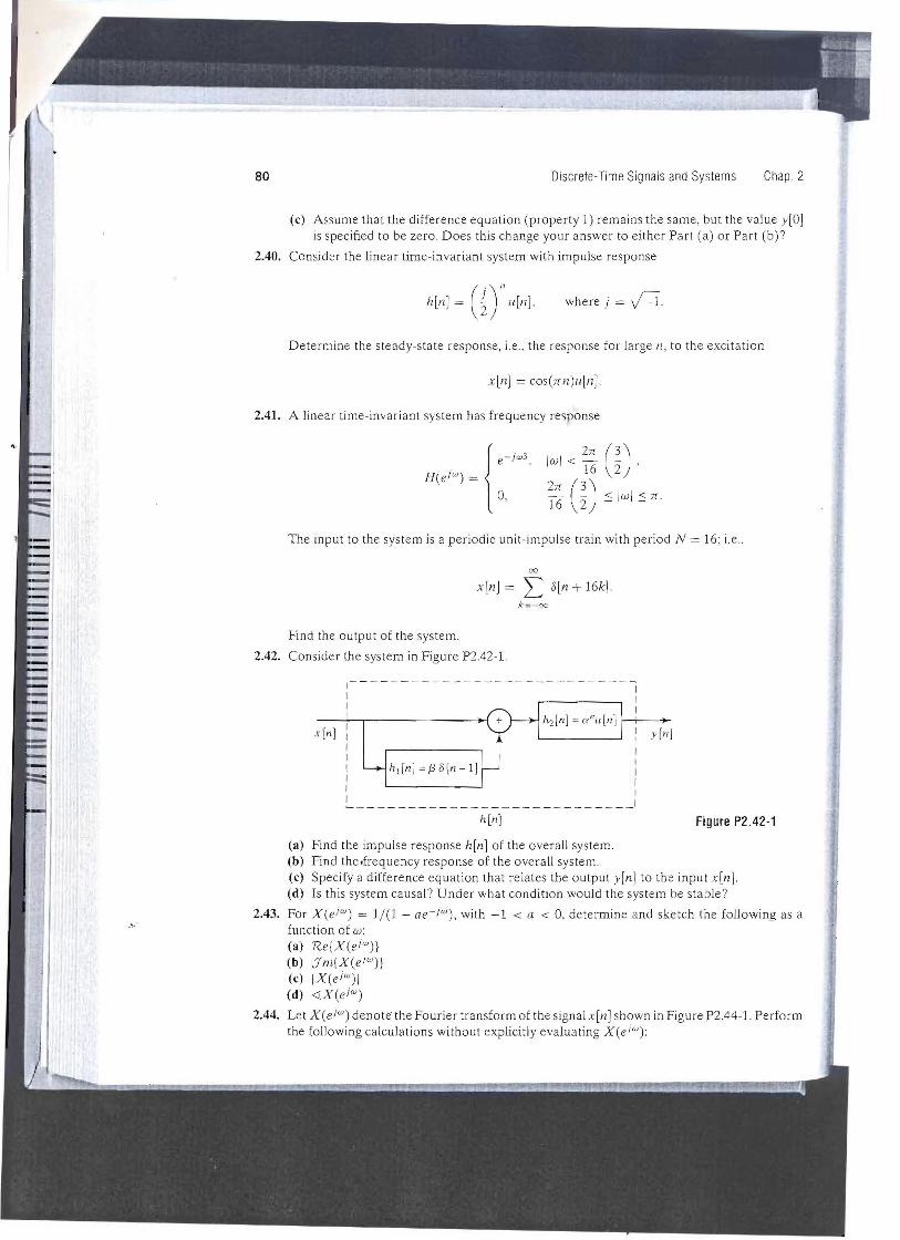
2.42. Consider the system in Figure P2.42-1.

1-------- - ------------------ ­1 1 1 1

1

h"2 [n] = Cl'nu[nll-t-~ x[n] 1

1 y[n] 1 1

1 ht [n]=/38[n-l] 1 I 1 I

~--------------------------~ h[n] Figure P2.42-1

(a) Find the impulse response h[nJ of the overall system. (b) Find the.frequency response of the overall sys tem . (c) Specify a difference equation that relates the output yin] to the input x[nJ. (d) Is this system causal? Under what condition would the system be stable?

2.43. For X(e io») = 1/ (1 - ae-/W ), with -1 < a < 0, determine and sketch the following as a

function of w: (a) Re(X(e/W

))

(b) Jm{X(eiw)} (c) IX(e/W)1 (d) «X(e j ''' )

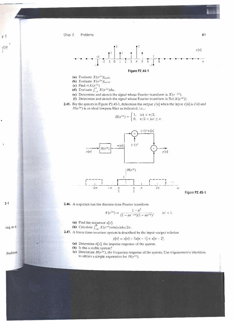
. 2.44. Let X(e io») denote the Fourier transform of the signal x[n] shown in Figure P2.44-1. Perform the following calcula tions without explicitly evaluating X(e i '''):

• • • • • • • • • • • • •

2-1

Chap. 2 Problems 81 p. 2

y[O] x[nJ

r l' r I 1'1 -2 -1 0 2 3 4 5 8 ----11-J

-3

6-J 7

Figure P2 .44-1

(a) Evaluate X(e iW )lw=o. (b) Evaluate X(e iW )lw=rr. (c) Find <f.X(eiw ) (d) Evaluate Drr X(e iw )dw.

(e) Determine and sketch the signal whose Fourier transform is X(e- iw). (1) Determine and sketch the signal whose Fourier transform is Re{X(e iw)}.

2.45. For the system in Figure P2AS-l , determine the output y[nJ when the input x[nJ is 3[n1 and H(eiw) is an ideallowpass filter as indicated , i.e.,

H(e iw) = {1 ' [Col < Jr /2, 0, Jr/2 < Iwl ::; Jr.

(-l)"w[I1J

W[I1J (_I)"

X [I1J

,-----, ,-----, , I ' , I '

-1T 1T !!. 1T (v

2 2 Figure P2.45-1

2.46. A sequence has the discrete-time Fourier transform

X( iw) _ 1 - a2

lal < 1.e - (1 _ ae- iw)(1 _ aeiw)'

(a) Find the seiuence x[n). ling as a (b) Calculate L" X(eI V» cos(w)dw/2Jr.

2.47. A linear time-invariant system is described by the input-output relation

y[n) = x[nJ + 2x[n - 1] + x[n - 2]. ..... (a) Determine h[n), the impulse response of the system .

(b) Is this a stable system? (c) Determine H(e iw ), the frequency response of the system. Use trigonometric identities

to obtain a simple expression for H(e iw ).

83

-. . .... ,

• ;r.. •

Chap. 2 Problems

2.52. The frequency response of an LTI system is

. De- H(e iw ) = e- iw/4 , -rr < w ::: rr .

Determine the output of the system, y[nJ, when the input is x[nJ = cos (Srrn j 2). Express fs tem your an swer in as simple a form as you ca n.

2.53. Consider the cascade of LTl discrete-time sys tems shown in Figure P2.S3-1.

y in] Figure P2 .53-1

The first system is described by the equation. trans-

Iwl < O.Srr ,Hl (eJOJ) = { 1,S(eiw) 0, O.Srr :::: Iwl < rr ,

yln] + and the second system is described by the equationunction

y[n] = w[n]- w[n -1]. anda > The input to this system is

~.imation x[nJ = cos(0.6rrn) + 38[n - S] + 2.

Determine th e output y[nJ. With careful thought , yo u will be able to use the properties ofponding LTI systems to write down the answer by inspection.

2.54. Consider an LTI system with frequ e ncy response

H(e JW ) = e-J[( w/2)+(rr / 4)1, -rr < w::: rr .

Determine y[n], the output of this system , if the input is

duration. x[n] = cos Cs;n -~)

for all n.

2.55. For the system shown in Figure P2.SS-I , System 1 is a memoryless nonlinear system. System 2 determines the value of A according to the rel a tion

:rmine the 100

;e hln]. A= L y [n].

11 = 0

x[n]

x[n] A Figure P2. 55-1

2.56.

Specifica lly. consider the class of inputs of the form x[nJ = cos(wn). with w a re al finite numbe r. Varyin g the value of w at the input will change A; i.e. , A will be a function of w . In general, will A be periodic in w? Justify your answer.

Consider a system S with input x[n] and output y[n] related according to the block diagram in Figure P2~S6-1.

system to the ..,. . X [/7] ----- ­ X y[n]

ulnJ. Figure P2. 56-1