Embed Size (px)
DESCRIPTION
Norme de reprezentare surse de poluare
Citation preview

7. Spatial mapping of emissions
EMEP/EEA emission inventory guidebook 2013 1
Category Title
General guidance Spatial mapping of emissions
Version Guidebook 2013
Lead authors
Nele Veldeman, Wim van der Maas
Contributing authors (including to earlier versions of this chapter)
John Van Aardenne, Justin Goodwin, Katarina Mareckova, Martin Adams, Paul Ruyssenaars,
Robert Wankmüller, Stephen Pye

7. Spatial mapping of emissions
EMEP/EEA emission inventory guidebook 2013 2
Contents
1 Introduction ............................................................................................................................... 3
2 Terminology .............................................................................................................................. 4
2.1 General terms ................................................................................................................... 4
2.2 Geographic features ......................................................................................................... 5
3 Methods for compiling a spatial inventory ............................................................................... 7
3.1 Compiling point source data ............................................................................................ 9
3.2 Computing diffuse emissions ......................................................................................... 11
3.3 Distributing diffuse emissions ....................................................................................... 12
3.4 Combining different spatial features .............................................................................. 34
4 Finding key spatial data sources ............................................................................................. 36
4.1 General ........................................................................................................................... 36
4.2 National datasets ............................................................................................................ 36
4.3 International datasets...................................................................................................... 38
5 Overview of available spatial emissions data.......................................................................... 42
6 References ............................................................................................................................... 44
7 Point of enquiry ....................................................................................................................... 45
7. Spatial mapping of emissions
EMEP/EEA emission inventory guidebook 2013 3
1 Introduction
The aim of this ‘Spatial emission mapping’ chapter is to further elaborate on the gridding of
emissions as to:
Support the link between emission data and air quality models that need emissions
information at a proper spatial, temporal and sectoral resolution;
Facilitate countries in (improving) the gridding of their emission inventories of air
pollutants under the United Nations Economic Commission for Europe (UNECE)
Convention on Long-range Transboundary Air Pollution (CLRTAP).
Sub-national spatial emissions are increasingly important because:
reported spatial emissions data are an input for models used to assess atmospheric
concentrations and deposition, as the spatial location of emissions determines to a great extent
their atmospheric dispersion patterns and impact area. The results of model assessments
inform national and international policies used to improve the environment and human health;
regular reporting of spatial emissions is required under the Emissions Reporting Guidelines
for Parties to the LRTAP Convention.
This chapter, developed by the European Environment Agency’s European Topic Centre on Air
Pollution and Climate Change Mitigation (EEA’s ETC/ACM), provides guidance on compiling
spatial emissions datasets. It focuses on methods suitable for generating and reporting spatial data
required under the LRTAP Convention that are consistent with nationally-reported inventories
under CLRTAP.
This chapter starts with the definition of terms used when dealing with spatial datasets (Section 2).
In Section 3 a generic set of methodologies for deriving spatial datasets from national emissions
inventories is established. A sector-specific tiered approach for estimating spatial emissions is
discussed, moreover, some sector-specific issues are dealt with. Furthermore, approaches to
combining spatial datasets are presented to enable the inventory compiler to derive an aggregated
spatial dataset combining sectoral emissions into a unified gridded dataset like that needed for
European Monitoring and Evaluation Programme (EMEP) reporting. All methods rely on the
identification and use of important spatial datasets. Therefore, generic data sources for this type of
data are outlined in Section 4. In Section 5 an overview of available spatially disaggregated
emission inventories, which could be used as an example, is given.
When preparing spatial data for reporting under EMEP, this chapter should be used in conjunction
with the EMEP Reporting Guidelines (1). These guidelines define the reporting requirements for
spatially resolved data.
The Reporting Guidelines give requirements concerning:
the EMEP grid (0.1° x 0.1° longitude/latitude);
the sectoral definitions for gridded and large point sources;
additional large point source information requirements, e.g. height class;
the required pollutants (main pollutants, PM, Pb, Cd, Hg, PAHs, HCB, dioxins/furans and
PCBs);
years for which reporting of gridded data is required.
(1) The Reporting Guidelines are available on the CEIP website (http://www.ceip.at)

7. Spatial mapping of emissions
EMEP/EEA emission inventory guidebook 2013 4
2 Terminology
2.1 General terms
CEIP - EMEP Centre on Emission Inventories and Projection (http://www.ceip.at).
CLRTAP - Convention on Long-range Transboundary Air Pollution.
Diffuse sources - Diffuse sources of a sector are defined as the national total of a sector minus the
reported point sources. This definition is in agreement with the definition used in E-PRTR (see
below) and implies that diffuse sources may contain (non reported) point sources, line sources,
and area sources.
EMEP - the Cooperative Program for Monitoring and Evaluation of the Long Range
Transmission of Air Pollutants in Europe.
EMEP grid - the EMEP grid is the geographical extent covering the EMEP area at a resolution of
0.1° × 0.1° longitude-latitude in the WGS84 geographic coordinate system. The domain covers the
geographic area between 30°N-82°N latitude and 30°W-90°E longitude.
E-PRTR - E-PRTR is the European Pollutant Release and Transfer Register, established under
EU Regulation (EC) No 166/2006 of the European Parliament and of the Council of 18 January
2006, and is intended to fully implement the obligations of the UNECE PRTR Protocol.
GIS - Geographical Information Systems.
HDV - Heavy Duty Vehicles, vehicles with a gross vehicle weight of > 3 500 kg.
IPPC - Integrated Pollution Prevention and Control. This EU Directive (the ‘IPPC Directive’)
imposes a requirement for industrial and agricultural activities with a high pollution potential to
have a permit which can only be issued if certain environmental conditions are met, so that the
companies themselves bear responsibility for preventing and reducing any pollution they may
cause. More recently, the Directive on Industrial Emissions 2010/75/EU (IED) was adopted by the
European Union. The IED replaces the IPPC Directive and a number of other sectoral directives as
of 7 January 2014, with the exception of the LCP Directive, which will be repealed with effect
from 1 January 2016.
LCPD - Large Combustion Plant Directive: Directive 2001/80/EC of the European Parliament and
of the Council of 23 October 2001 on the limitation of emissions of certain pollutants into the air
from large combustion plants.
LDV - Light Duty Vehicles, vehicles with a gross vehicle weight of ≤ 3 500 kg.
NACE - Classification of Economic Activities in the European Union.
NFR - Nomenclature For Reporting.
NUTS - Nomenclature of Units for Territorial Statistics, which is a hierarchical classification of
administrative boundaries developed by Eurostat. The idea behind NUTS is to provide a common
designation for different levels of administrative geographic boundaries across the EU regardless
of local language and naming conventions.
SNAP - Selected Nomenclature for sources of Air Pollution — developed as part of the
CORINAIR project for distinguishing emission source sectors, sub-sectors and activities.
7. Spatial mapping of emissions
EMEP/EEA emission inventory guidebook 2013 5
Surrogate spatial dataset - a geographically resolved dataset of statistics by grid, link, point or
boundary such as land use coverage percentage by grid, vehicle flow by road link, employers
number by industrial point, population by administrative boundary. Applied as alternative data
source to spatially allocate emissions, when direct spatial information on the emission source is
not available.
2.2 Geographic features
Geographical features will be used to represent emission sources. These features will define the
geographical structure of the spatial dataset.
Point sources: A point source is an emission source at a known location, represented by x and y
coordinates that indicate the main point of emission. Examples of point sources are industrial
plants or power stations.
Emissions from point sources represent sectors of a national inventory either fully (e.g. often for
power stations where the sector is made up of only large sites for which emissions reporting is
mandatory) or in part (e.g. such as combustion in industry, for which only the large sites within
the sector are typically required to report emissions). In the latter case, the remainder of the
emissions for the sector are mapped as an area source.
Large point sources (LPS): LPS are defined in the UNECE reporting guidelines (1) as
facilities whose combined emissions, within the limited identifiable area of the site
premises, exceed certain pollutant emission thresholds. Note: although stack height is an
important parameter for modelling emissions, it is not a criterion used for selecting LPS.
Area sources: An area source is an emission source that exhibits diffuse characteristics. For
example, sources that are too numerous or small to be individually identified as point sources or
from which emissions arise over a large area. This could include forests, residential areas and
administrative/commercial activities within urban areas.
Area sources as polygons: area polygons are often used to represent data attributed to
administrative or other types of boundaries (data collection boundaries, site boundaries
and other non-linear or regular geographical features).
Residential fuel combustion is an example of a sector that can be represented in this way,
using population census data mapped using the polygons defining the data collection
boundaries.

7. Spatial mapping of emissions
EMEP/EEA emission inventory guidebook 2013 6
Polygons are vector- (line-) based features and are characterised by multiple x, y
coordinates for each line defining an area. Examples of areas defined by polygons are the
regions as defined by the NUTS classification (Nomenclature of Units for Territorial
Statistics). According to this classification, the economic territory of the EU is divided in
several zones, presented by polygons:
NUTS 1: major socio-economic regions
NUTS 2: basic regions for the application of regional policies
NUTS 3: small regions for specific diagnoses
Area sources as grids: area sources can be represented in a regular grid of
identically-sized cells (either as polygons or in a raster dataset). The spatial aspects of
grids are usually characterised by geographical coordinates for the centre or corner of the
grid and a definition of the size of each cell.
Agricultural and natural emissions sectors can be represented using land use data derived
from satellite images in raster format.
Grids are often used to harmonise datasets: point, line and polygon features can be
converted to grids and then several different layers of information (emission sources) can
easily be aggregated together (see section 3.4).
Line sources: A line source is an emission source that exhibits a line type of geography, e.g. a
road, railway, pipeline or shipping lane. Line sources are represented by vectors with a starting
node and an end node specifying an x, y location for each. Line source features can also contain
vertices that define curves between the start and end reference points.
7. Spatial mapping of emissions
EMEP/EEA emission inventory guidebook 2013 7
3 Methods for compiling a spatial inventory
This section provides general guidance on the approaches to deriving spatially resolved (e.g.
sub-national) datasets. First, an introduction on general good practice is given. Consequently, a
concrete approach is outlined. Hereto, a schematic overview of consecutive steps is provided (see
Figure 3-1). The different steps as outlined in the scheme are then discussed in more detail in
separate paragraphs.
It is good practice to consider the elements below when defining an efficient spatial distribution
project.
1. Use key category analysis (see Chapter 2, Key category analysis and methodological choice)
to identify the most important sources and give the most time to these.
2. Make use of GIS tools and skills to improve the usefulness of available data. This will mean
understanding the general types of spatial features and possibly bringing in skills from outside
the existing inventory team for the production/manipulation of spatial datasets.
3. Make use of existing spatial datasets and carefully consider the merits versus costs of
extensive new surveying or data processing to derive new spatial datasets. It is often more
important to generate a timely dataset based on less accurate data than a perfect dataset that
means reporting deadlines are missed or all resources are consumed.
4. Select the surrogate data that is judged to most closely represent the spatial emissions patterns
and intensity, e.g. for combustion sources, surrogate spatial datasets that most closely match
the spatial patterns of fuel consumed by type should be chosen.
5. Surrogate spatial datasets that are complete (cover the whole national area) should be
preferred.
6. Use, when possible and when no other more accurate data is available, the spatial surrogate
that was used for spatial mapping in previous years. This is to guarantee consistency.
7. Issues relating to non-disclosure may be encountered (at a sectoral or spatial level) that may
impose barriers to acquiring data (e.g. population, agriculture, employment data). As only
highly aggregated output data is needed for reporting, signing of non-disclosure or
confidentiality agreements or asking the data supplier to derive aggregated datasets may
improve the accessibility of this data. It is important that issues relating to this are identified
and dealt with in consultation with the national statistical authority.
8. It is advisable to consider the resolution (spatial detail) required in order to meet any wider
national or international uses. Aggregation to the present EMEP 0.1 x 0.1 degree
longitude/latitude grid could be done, for example, from more detailed spatial resolutions that
might be more useful in a national context. Most nationally reported emissions datasets are
based on national statistics and are not resolved spatially in a manner that could be readily
disaggregated to the required 0.1 x 0.1 degree EMEP grid. Possible exceptions in some
countries are detailed road transport networks and reported point source emissions data..
9. When updating a spatial inventory it is often not possible to update all the spatial datasets
every year (for economical reasons). A yearly data acquisition plan (DAP) can describe
which surrogate data is updated with which frequency, depending on its importance, costs and
variation in time.
10. When the budget is very limited the available datasets in section 5 can act as a starting point
when they are used as a surrogate data for the spatial allocation of the national total for some
sectors. The limited resources can then be used for the most relevant sectors.

7. Spatial mapping of emissions
EMEP/EEA emission inventory guidebook 2013 8
Different methods for compiling spatially resolved estimates can be used depending on the
availability of data. However, the general approach always contains the same basic steps.
Therefore, a general scheme can be followed. The schematic overview is presented in Figure 3-1.
Figure 3-1 General approach for compiling a spatial emission inventory
First, an emissions inventory for point sources should be compiled. Hereto, a number of different
data sources are available. In general, for many European countries, the best starting point is the
European Pollutant Release and Transfer Register (E‐PRTR) database, which has been established
by Regulation 166/266/EC from 18 January 2006. It should be noted that E-PRTR is based on data
officially submitted by national competent authorities, and so internal national contact points will
be able to provide point source data. In other countries, many industrial point sources and their
emission reports are similarly available through the relevant national or regional competent
authorities, especially for those countries that are Parties to the UNECE Aarhus Convention PRTR
protocol. In order to obtain a comprehensive point source emissions inventory, the E-PRTR or
other point source emissions should however be combined with emissions stemming from point
sources that are regulated but for which there are no annual emissions reporting requirements and
from point sources for sites or pollutants not reported or regulated. In section 3.1 a specific
method for compiling point source data is described.
In a second step, the shares of releases from diffuse sources should be determined. The point
source emissions compiled in the first step should not exceed national total emissions reported
under LRTAP Convention, which include all anthropogenic emissions occurring in the
geographical area of the country (large point sources, linear and area sources). However, due to
inconsistent reporting under different reporting obligations and due to different sector
National reported emissions dataset
(NFR 09 categories)
1. Compile emissions for point sources
See § 3.1
2. Compute diffuse emissions
by subtracking the emissions from the
facilities from the national totals
See § 3.2
Spatially resolved emission map
of point sources
Consistency check:
diffuse emissions > 0?No Yes
All emissions can be
allocated to point
locations
3. Spatially disaggregate the diffuse emissions
See § 3.3
Spatially resolved emission
map of line sources
Spatially resolved emission
map of area sources
4. Combine different spatial features
See § 3.4
Spatially disaggregated
emissions map
National reported point source emissions
(E-PRTR Annex I activities)

7. Spatial mapping of emissions
EMEP/EEA emission inventory guidebook 2013 9
classification systems, point source emissions might exceed the national totals. Therefore, linking
national point source data and national total emissions turns out to be a challenging task:
computation of diffuse emissions is not as straightforward as a simple subtraction per sector. In
section 3.2 some guidance to develop a subtraction methodology for diffuse emissions to air is
outlined.
Once the national diffuse emission totals are determined per source category, a gridding
methodology for each category should be developed. National emission estimates will need to be
distributed across the national spatial area using a surrogate spatial dataset, according to a
common basic principle which can be presented in a straightforward formula that is referring to
the specific surrogate spatial dataset. The methods used can range in quality from Tier 3 to Tier 1
depending on the appropriateness of the spatial activity data being used. An extensive description
of the basic principle and the different methodologies is provided in section 3.3. Furthermore
sectoral guidance is given and some examples are listed.
Finally, different spatial features need to be combined, in order to obtain a spatially disaggregated
emissions map. Information on how this could be done is provided in section 3.4.
3.1 Compiling point source data
Emissions for point sources can be compiled using a number of different data sources and
techniques. For convenience, the point source data can be divided into three groups.
1. Regulated point sources such as those regulated under the Integrated Pollution Prevention
and Control (IPPC) Directive regulatory regime and/or where there is a requirement for
centralised annual emissions reporting (e.g. for E-PRTR/the Large Combustion Plant
(LCP) Directive);
2. Point sources that are regulated but for which there are no annual emissions reporting
requirements (e.g. E-PRTR does not cover all point source emissions as it uses emission
thresholds, emissions below the specified threshold are not included);
3. Point sources for sites or pollutants not reported or regulated.
To obtain a detailed point source emission data set, point source emissions of all three groups
should be combined.
First the regulated point sources with requirement for reporting should be considered. As
outlined in the introduction, the best starting point is the E‐PRTR or equivalent national database.
Such data can be used directly: emission data are known at exact locations, represented by x and
y coordinates indicating the main point of emission on the site. As such there is no need to further
spatially disaggregate the data to obtain spatially resolved emission maps of point sources per
specific sector.
The E-PRTR or equivalent national data represent the total annual emission releases during
normal operations and accidents. For E-PRTR, releases and transfers must however be reported
only if the emissions of a facility are above the activity and pollutant thresholds set out in the
E-PRTR Regulation. Therefore, sources may not need to report emissions if these are below a
specified reporting threshold or reporting is not required for the specific activity undertaken at a
facility. Consequently point source emissions from smaller plants or from specific activities might
not be included in the E-PRTR database.

7. Spatial mapping of emissions
EMEP/EEA emission inventory guidebook 2013 10
Emissions from regulated point sources without annual emissions reporting requirements can
however often be estimated based on centralised data on process type and/or registered capacities
and initialisation reports associated with the original application for emission permits. Estimating
point source emissions for non E-PRTR sources and representing them with x and y coordinates
according to their exact location, results in spatially resolved maps of the smaller point sources.
In some cases, data sets are not complete. Furthermore, some point sources are not regulated.
Emissions from not reported or non-regulated sources can be modelled by distributing national
emission estimates over the known sources on the basis of capacity, pollutant correlations with
reported data (e.g. particulate to PM10/PM2.5) or some other 'surrogate' statistic, such as
employment. The following box (Example 1) provides some examples of approaches used to
derive emissions for point sources in the absence of reported data.
EXAMPLE 1: ESTIMATING POINT SOURCE EMISSIONS FOR SOURCES/POLLUTANTS THAT ARE NOT REPORTED
In some cases, datasets are not complete. Furthermore, some point sources are not regulated. In these
cases, point source data is generated using national emission factors and some ‘surrogate’ activity
statistic. Examples of approaches used are given below.
Estimates of plant capacity can be used to allocate the national emission estimate. This approach
can be used, for example, for bread bakeries where estimates of the capacity of large mechanised
bakeries can be made or gathered from national statistics or trade associations.
Emission estimates for one (reported) pollutant can be used to provide a weighted estimate of the
national emission estimate of another pollutant. For example, emissions of PM10 from certain
coating processes can be estimated by allocating the national total to sites based on their share of
the national VOC emission.
Deriving point source estimates based on pollutant ratios can be used to fill gaps in reported
emissions data. In some cases known PM10/PM2.5 ratios can be established to estimate emissions
for PM10 and PM2.5 for similar processes. Where no other data is available, other pollutants, such
as NOx and SO2, can be used to distribute other pollutant emissions.
Assuming that all plants in a given sector have equal emissions: in a few cases where there are
relatively few plants in a sector but no activity data can be derived, emissions can be assumed to
be equal at all of the sites.
With the possible exception of using plant capacity, many of the approaches listed above will yield
emission estimates that are subject to significant uncertainty. However, most of the emission estimates
generated using these methods are, individually, relatively small and the generation of point source
data by these means is judged better than mapping the emissions as area sources.
Finally, the obtained point source inventories and maps of the three different groups should be
combined. It is therefore recommended to compile the different data sets based on the same sector
classification. In principle any classification can be chosen initially, however, it is advisable to
consider the categories required under different reporting obligations when compiling the point
source emission data. The derived point source datasets should be structured such that it is
possible to differentiate point source emissions into the relevant reporting sectors.
According to E-PRTR regulations, point source emissions have to be reported in categories
covering 65 economic activities within 9 different industrial sectors. In order to allow computation
of diffuse emissions, the E-PRTR or equivalent national LPS emission data will however need to
be reconciled with the national totals and sectoral definitions in the inventory as reported under
CLRTAP. Hereto, the data will need to be classified into process or Nomenclature For Reporting
(NFR) categories (see section 3.2). Therefore it might be advisable to model and/or estimate non

7. Spatial mapping of emissions
EMEP/EEA emission inventory guidebook 2013 11
reported emissions (group 2 and 3) using the E-PRTR and/or NFR categories as well. Also, it
might be worth to consider any other national or international uses, before deciding on the sector
classification. The following link maps different classifications from the various reporting
obligations:
http://www.ceip.at/fileadmin/inhalte/emep/xls/Spreadsheet_for_reporting_formats.xls.
As outlined in the introduction, the purpose of spatial emission mapping is twofold. On one hand,
countries are obliged to report gridded emissions under the LRTAP Convention. On the other
hand, spatial emission maps are crucial input to air quality models. With respect to the latter, an
important note should be made. For modelling purposes, source characteristics such as stack
height, source diameter and source heat capacity are important parameters. Nevertheless these
characteristics are not required under most reporting obligations, it is highly recommended to
include them when compiling the national point source emission inventory for modelling
purposes.
3.2 Computing diffuse emissions
Point source emissions, as compiled in the first step, represent sectors of a national inventory
either fully or partly. In the latter case the remaining emissions are to be considered as diffuse
emissions. Therefore a methodology to distinguish the point-source releases and diffuse releases
needs to be developed.
Review of different datasets (e.g. E-PRTR inventory versus CLRTAP inventory) can reveal that
the total or sector specific E‐PRTR emissions of some countries exceed the emissions officially
reported by the same countries to CLRTAP (e.g. CEIP, 2010). If this occurs, a straightforward
subtraction could not be used. Instead of developing potentially complicated procedures to
overcome this problem, it is strongly advised to first solve the issue before moving further in the
process of spatial disaggregation of emissions. As the problem might occur due to different
reasons and as it is impossible to provide a check list covering all causes, only some general
guidance can be given in this section.
In most cases, exceedances of national totals by point emissions are caused by:
inconsistent reporting under different reporting obligations;
different sector classification systems;
missing data (e.g. not all point sources included in national total);
inconsistent data updates.
It is therefore suggested to first compare the different reporting obligations, making sure the same
activities are taken into account. Furthermore, it should be checked whether the sector
classifications are applied in a consistent manner (e.g. quite often total E-PRTR emissions do not
exceed the national total whereas sector specific totals do, and this can be a consequence of
inconsistent sector conversions). Moreover, it is advised to check whether the point source
contribution in the national total equals the totals that are effectively reported to E-PRTR. It might
be that the point source data were revised after reporting to E-PRTR, and that the update is only
taken into account in the national totals.
Different methodologies to identify the diffuse shares of the national emissions (CLRTAP) which
are not covered by the reporting to E-PRTR have been developed in the past. In all approaches,
firstly the different categorizations (NFR for CLRTAP and Annex I E-PRTR) used for reporting
requirements, have been analysed. Based on this correlation of activities (link NFR – E-PRTR)

7. Spatial mapping of emissions
EMEP/EEA emission inventory guidebook 2013 12
several subtraction approaches have been applied. An overview of different procedures can be
found in Theloke et al., 2009.
Some European countries (e.g. BE, NL or UK) already apply methods to identify sector specific
shares of diffuse emissions. Additional information can be obtained via contacting emission
experts in these countries.
3.3 Distributing diffuse emissions
There will be many cases where emissions cannot be calculated at a suitably small spatial scale or
estimates are inconsistent with national estimates and statistics. Hence, national emission
estimates will need to be distributed across the national spatial area using a surrogate spatial
dataset. The methods used can range in quality from Tier 3 to Tier 1 depending on the
appropriateness of the spatial activity data being used, the basic principle behind the different
methods is however the same for all cases. In this section, both, the basic principles as some
derived methodologies are outlined.
3.3.1 Basic principles
The basic principle of distributing emissions is presented in the formula below using a
surrogate spatial dataset x:
ix
jx
ix
tix
value
valueemissionemission
Where:
i : is a specific geographic feature;
emissionix : is the emissions attributed to a specific geographical feature (e.g. a
grid, line, point or administrative boundary) within the spatial
surrogate dataset x;
emissiont : is the total national emission for a sector to be distributed across
the national area using the (x) surrogate spatial dataset;
valueix – jx : are the surrogate data values of each of the specific geographical
features within the spatial surrogate dataset x.
The following steps should be followed:
1. determine the emission total to be distributed (emissiont) (either national total for sector
or where a sector is represented by some large point sources: national total — sum of
point sources, as outlined in sections 3.1 and 3.2);
2. distribute that emission using the basic principals above using a suitable surrogate statistic
(according to the detailed guidance by sector given below).
7. Spatial mapping of emissions
EMEP/EEA emission inventory guidebook 2013 13
3. Keep the surrogate spatial data in its original shape as long as possible in the calculation.
This makes it easy to correct for mistakes or add new information without a big effort
later on.
This approach effectively shares out the national emissions according to the intensity of a
chosen or derived spatially resolved statistic.
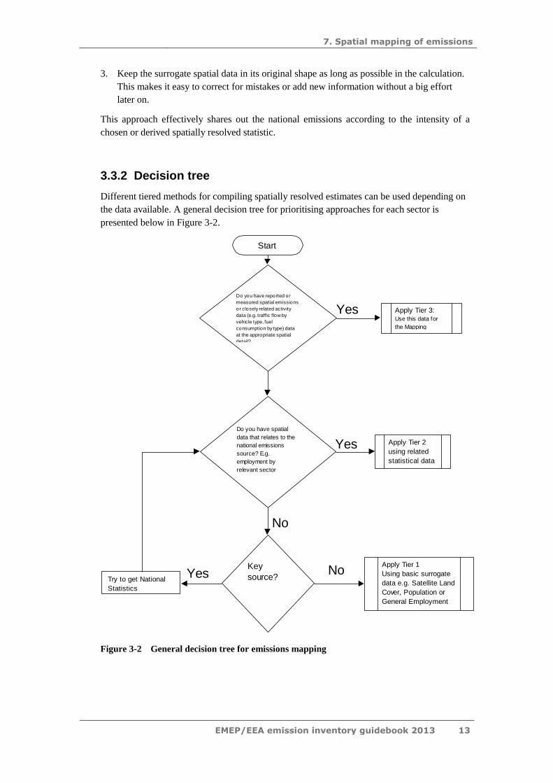
3.3.2 Decision tree
Different tiered methods for compiling spatially resolved estimates can be used depending on
the data available. A general decision tree for prioritising approaches for each sector is
presented below in Figure 3-2.
Figure 3-2 General decision tree for emissions mapping
Start
Do you have reported or
measured spatial emissions
or closely related activity
data (e.g. traffic flow by
vehicle type, fuel
consumption by type) data
at the appropriate spatial
detail?
Apply Tier 3:Use this data for
the Mapping
Do you have spatial
data that relates to the
national emissions
source? E.g.
employment by
relevant sector
Apply Tier 2
using related
statistical data
Key
source?Try to get National
Statistics
Apply Tier 1
Using basic surrogate
data e.g. Satellite Land
Cover, Population or
General Employment
Yes
Yes
Yes
No
No

7. Spatial mapping of emissions
EMEP/EEA emission inventory guidebook 2013 14
Tier 3 methods will include estimates that are based on closely related spatial activity
statistics, e.g. road traffic flows by vehicle type, spatial fuel consumption data by sector (e.g.
boiler use data).
Tier 2 methods will be based on the use of surrogate statistics. However, for Tier 2, these
statistics need to relate to the sector and could include detailed sector specific employment,
population or household size and number (for domestic emissions).
Tier 1 methods will include the use of loosely related surrogate statistics such as urban rural
land cover data, population (for non domestic sources).
These principals apply to the general methods for estimating spatial emissions. Detailed
methods are provided for each sector in section 3.3.3. The following box (Example 2)
provides some general examples of distributing national emissions.
EXAMPLE 2: DISTRIBUTION OF NATIONAL EMISSIONS
SO2 emissions from residential combustion may be allocated based on a gridded or administrative
boundary (e.g. NUTS) spatial dataset of population density. However, emissions of SO2 may not
correlate very well to population density in countries where a variety of different fuels are burned
(e.g. city centres may burn predominantly gas and therefore produce very low SO2 emissions per
head of population). Additional survey information and or energy supply data (e.g. metered gas
supply) could be used to enhance the population-based surrogate for residential emissions and
achieve a better spatial correlation to ‘real’ emissions.
National transport emissions may be allocated to road links (road line maps) based on measured or
modelled traffic flow, road type or road width information for each of the road links. Again, the
closer the distribution attributes for each road link correlate to the actual emissions, the better. For
example, road width and road type only loosely relate to traffic emissions and provide a poor
distribution method. Being able to distinguish between the numbers of heavy goods vehicles and
cars using different road links each year, and the average speeds of traffic on these links, will
improve the compiler’s ability to accurately allocate emissions.
In many cases the combination of more than one spatial dataset will provide the best results
for distributing emissions. For example, where traffic count/density information is not
available, basic road link information can be combined with population data to derive
appropriate emission distribution datasets to provide a Tier 1 methodology.

7. Spatial mapping of emissions
EMEP/EEA emission inventory guidebook 2013 15
3.3.3 Sectoral guidance
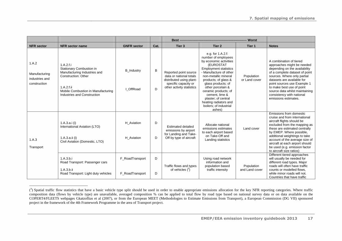
Table 1 gives general guidance for the tiered mapping of emissions for different sectors. The
first two columns list and describe the NFR sector codes. The third column reveals the
corresponding GNFR sector (2). The fourth column gives an indication on whether the sector
is fully, partly, or not covered by E-PRTR point sources, by assigning a category (A-D) to
each NFR sector. All NFR categories are represented with the following corresponding
categories:
A – E-PRTR point source relevant: covered by E-PRTR sources
B – E-PRTR point source relevant: covered by E-PRTR sources but also including
diffuse sources (below E-PRTR reporting threshold)
C – E-PRTR relevant like industrial facilities (B), but only agricultural installations
D – Diffuse sources, which are not covered by E-PRTR
This gives a clear indication on whether diffuse emissions that need spatial disaggregation are
to be expected.
Moreover, Table 1 contains a sector specific overview of different spatial mapping approaches
ranging from Tier 3 to Tier 1.
(
2) http://www.ceip.at/reporting-instructions/ - table for mapping between GNFR and NFR

7. Spatial mapping of emissions
EMEP/EEA emission inventory guidebook 2013 16
Table 1: General tiered guidance for the spatial distribution of emissions by sector
Best -------------------------------------------------------------- Worst
NFR sector NFR sector name GNFR sector Cat. Tier 3 Tier 2 Tier 1 Notes
1.A.1
Energy industries
1.A.1.a Public Electricity and Heat Production
A_PublicPower A
Reported point source data or national totals distributed using plant-
specific capacity or other activity statistics
Employment data
e.g. for 1.A.1.c: number of employees by economic activities
(EUROSTAT Employment statistics - Manufacture of coke
oven products)
See also section 3.3.4.2 for an
example
Land cover
A combination of tiered approaches might be needed depending on the availability of a complete dataset of point sources. Where only partial datasets are available for point sources use Example 1 to make best use of point source data whilst maintaining consistency with national emissions estimates.
1.A.1.b Petroleum Refining
B_Industry A
1.A.1.c Manufacture of Solid Fuels and Other Energy Industries
B_Industry B
1.A.2
Manufacturing
industries and
construction
1.A.2.a Stationary Combustion in Manufacturing Industries and Construction: Iron and Steel
B_Industry B
Reported point source data or national totals distributed using plant-
specific capacity or other activity statistics
Employment data
e.g. for 1.A.2.a: number of employees by economic activities
(EUROSTAT Employment statistics - Manufacture of basic iron and steel and of
ferroalloys)
Population or Land cover
A combination of tiered approaches might be needed depending on the availability of a complete dataset of point sources. Where only partial datasets are available for point sources use Example 1 to make best use of point source data whilst maintaining consistency with national emissions estimates.
1.A.2.b Stationary Combustion in Manufacturing Industries and Construction: Non-ferrous Metals
B_Industry B
1.A.2.c Stationary Combustion in Manufacturing Industries and Construction: Chemicals
B_Industry B
1.A.2.d Stationary Combustion in Manufacturing Industries and Construction: Pulp, Paper and Print
B_Industry B
1.A.2.e Stationary Combustion in Manufacturing Industry and Construction: Food Processing, Beverages and Tobacco
B_Industry B
7. Spatial mapping of emissions
EMEP/EEA emission inventory guidebook 2013 17
Best -------------------------------------------------------------- Worst
NFR sector NFR sector name GNFR sector Cat. Tier 3 Tier 2 Tier 1 Notes
1.A.2
Manufacturing
industries and
construction
1.A.2.f.i Stationary Combustion in Manufacturing Industries and Construction: Other 1.A.2.f.ii Mobile Combustion in Manufacturing Industries and Construction
B_Industry
I_OffRoad
B
D
Reported point source data or national totals distributed using plant-
specific capacity or other activity statistics
e.g. for 1.A.2.f:
number of employees by economic activities
(EUROSTAT Employment statistics - Manufacture of other non-metallic mineral products; of glass & glass products; of other porcelain &
ceramic products; of cement, lime &
plaster; of central heating radiators and boilers; of industrial
ashes)
Population or Land cover
A combination of tiered approaches might be needed depending on the availability of a complete dataset of point sources. Where only partial datasets are available for point sources use Example 1 to make best use of point source data whilst maintaining consistency with national emissions estimates.
1.A.3 Transport
1.A.3.a.i (i) International Aviation (LTO) 1.A.3.a.ii (i) Civil Aviation (Domestic, LTO)
H_Aviation
H_Aviation
D
D
Estimated detailed emissions by airport
for Landing and Take-Off by type of aircraft
Allocate national emissions estimates to each airport based
on Take-Off and Landing statistics
Land cover
Emissions from domestic cruise and from international aircraft flights should be excluded from the mapping as these are estimated centrally by EMEP. Where possible, additional weightings to take account of the average size of aircraft at each airport should be used (e.g. emission factor to aircraft size ratios)
1.A.3.b.i Road Transport: Passenger cars 1.A.3.b.ii Road Transport: Light duty vehicles
F_RoadTransport
F_RoadTransport
D
D
Traffic flows and types of vehicles (
3)
Using road network
information and population based
traffic intensity
Population and Land cover
Different tiered approaches will usually be needed for different road types. Major roads will often have traffic counts or modelled flows, while minor roads will not. Countries that have traffic
(3) Spatial traffic flow statistics that have a basic vehicle type split should be used in order to enable appropriate emissions allocation for the key NFR reporting categories. Where traffic
composition data (flows by vehicle type) are unavailable, averaged composition % can be applied to total flow by road type based on national survey data or on data available on the
COPERT4/FLEETS webpages Gkatzoflias et al (2007), or from the European MEET (Methodologies to Estimate Emissions from Transport), a European Commission (DG VII) sponsored
project in the framework of the 4th Framework Programme in the area of Transport project.

7. Spatial mapping of emissions
EMEP/EEA emission inventory guidebook 2013 18
Best -------------------------------------------------------------- Worst
NFR sector NFR sector name GNFR sector Cat. Tier 3 Tier 2 Tier 1 Notes
1.A.3 Transport
1.A.3.b.iii Road Transport: Heavy duty vehicles 1.A.3.b.iv Road Transport: Mopeds & Motorcycles 1.A.3.b.v Road Transport: Gasoline evaporation 1.A.3.b.vi Road Transport: Automobile tyre and brake wear 1.A.3.b.vii Road Transport: Automobile road abrasion
F_RoadTransport
F_RoadTransport
F_RoadTransport
F_RoadTransport
F_RoadTransport l
D
D
D
D
D
Traffic flows and types of vehicles
Using road network information and
population based traffic intensity
Population and Land cover
count/flow information will usually need to apply a Tier 2 method for minor roads Different tiered approaches will usually be needed for different road types. Major roads will often have traffic counts or modelled flows, while minor roads will not. Countries that have traffic count/flow information will usually need to apply a Tier 2 method for minor roads
1.A.3.c Railways
I_Offroad
D
Diesel rail traffic on the rail network reconciled with national mobile
locomotive consumption data
Rail network and population-based traffic weightings
Population-weighted
distributions of land cover class
for rail
Rail networks that have been electrified should be excluded from the distributions where possible. This may only be important if large areas are all electrified (e.g. cities)
1.A.3.d.i (i) International maritime Navigation 1.A.3.d.i (ii) International inland waterways 1.A.3.d.ii National Navigation (Shipping)
z_Memo
G_Shipping
G_Shipping
D
D
D
Route-specific ship movement data and details of fuel quality
by region, consumption and
emission factors by type of ship & fuel
Port arrival & destination statistics used to weight port
and coastal shipping areas
Assign national emissions to Land cover classes for ports and coastal shipping areas
Tier 1 & 2 methods will need to make assumptions about the weighting of in-port vs. In-transit emissions. Tier 3 methods will need to use ship movement data from centralised databases and account for in port emissions for loading and unloading of ships. Harbourmaster or coast guard data can sometimes provide details of ship time in ports and operations. Emissions will need to be broken down into national and
7. Spatial mapping of emissions
EMEP/EEA emission inventory guidebook 2013 19
Best -------------------------------------------------------------- Worst
NFR sector NFR sector name GNFR sector Cat. Tier 3 Tier 2 Tier 1 Notes
1.A.3 Transport
international data. Useful information for the mapping of shipping data can be obtained from Entec UK (2005).
1.A.3.e Pipeline compressors
B_Industry D Reported/collected
data Land cover Land cover
1.A.4
Other sectors
1.A.4.a.i Commercial / Institutional: Stationary 1.A.4.a.ii Commercial / Institutional: Mobile
C_OtherStationary Comb
I_OffRoad
D
D
Reported/collected point source data, boiler census or
surveys
Employment for public and commercial
services
Land cover
Large point source data is likely to be minimal unless there are large district heating or commercial/institutional heating plant included in the national inventory under sectoral 1A4a
1.A.4.b.i Residential: Stationary plants 1.A.4.b.ii Residential: Household and gardening (mobile)
C_OtherStationary
Comb
I_OffRoad
D
D
Detailed fuel deliveries for key fuels (e.g.gas)
and modelled estimates for other fuels using data on population density and/or household
numbers and types.
Population or household density combined with land cover data if smoke control areas exist in
cities.
Land cover
Tier 1 & 2 methods assume that a linear relationship between emissions and population density or land cover exists. This assumption will be most realistic if a country has a uniform distribution of fuel use by type. Where there is a broad variation of fuel type use in different areas, the accuracy of the simple method will be much lower
1.A.4.c.i Agriculture/Forestry/Fishing: Stationary 1.A.4.c.ii Agriculture/Forestry/Fishing: Off-road Vehicles & Other Machinery
C_OtherStationary Comb
I_OffRoad
D
D
For 1.A.4.c.i and 1.A.4.c.ii:
Detailed fuel deliveries for key fuels (e.g. gas)
and modelled estimates for other
fuels using employment data
For 1.A.4.c.i and 1.A.4.c.ii:
Employment data for the agricultural and
forestry sectors
Land cover
Where land cover is used, emissions for agriculture and forestry should be split and distributed according to the relevant classes. Where this is not possible, emissions should be distributed according to a combined land cover class for agriculture and forests or allocated to the dominant class e.g. ‘arable land’ for countries where emissions from agricultural combustion dominate.

7. Spatial mapping of emissions
EMEP/EEA emission inventory guidebook 2013 20
Best -------------------------------------------------------------- Worst
NFR sector NFR sector name GNFR sector Cat. Tier 3 Tier 2 Tier 1 Notes
1.A.4.c.iii Agriculture/Forestry/Fishing: National Fishing
G_Shipping
D
For 1.A.4.c.iii: Allocation of
emissions to ports on fish landings and to geographic areas of
fishing grounds
For 1.A.4.c.iii: Allocation of
emissions to ports on fish landings
For 1.A.4.c.iii: Assign national
emissions to Land cover classes for
ports.
Where employment data is used, care should be taken to ensure that the employment classes are representative of the national sector for Agriculture and Forestry. Employment statistics will often include the financial and administrative head offices (often located in cities) while energy statistics based national emissions from these ‘head offices’ may be included under 1.A.4.a.i Commercial / Institutional: Stationary. Care should be taken to ensure that the emissions are located where they occur. The use of employment data will locate emissions at registered places or regions of work and may tend to focus emissions inappropriately to urbanised areas Emissions from fishing are likely to be associated with fishing grounds rather than port activities. Tier 3 methods will need to allocate emissions to ports and fishing grounds
1.A.5
Other
1.A.5.a Other, Stationary (including Military)
C_OtherStationary Comb
D
Population and Land cover
Population and Land cover
Population
and Land cover
1.A.5.b Other mobile (Incl. military, land based & recreational boats).
I_OffRoad D

7. Spatial mapping of emissions
EMEP/EEA emission inventory guidebook 2013 21
Best -------------------------------------------------------------- Worst
NFR sector NFR sector name GNFR sector Cat. Tier 3 Tier 2 Tier 1 Notes
1.B.1
Fugitive
emissions from
solid fuels
1.B.1.a Fugitive emission from Solid Fuels: Coal Mining and Handling 1.B.1.b Fugitive emission from Solid Fuels: Solid Fuel Transformation 1.B.1.c Other fugitive emissions from solid fuels
D_Fugitive
D_Fugitive
D_Fugitive
B
B
B
Reported point source data or using plant-specific capacity or
other activity statistics
Locate point sources and use employment
data for specific sectors to allocate
emissions
e.g. for 1.B.1.b: number of employees by economic activities
(EUROSTAT Employment statistics
- Electric power generation, transmis-sion and distribution; Manufacture of coke
oven products)
Total employment for the mining and
transformation industry as a
whole
Mines, fuel transformation plant, depots and distribution centres are likely to be regulated and significant national industrial sites. In these cases site-specific information can be collected and used to distribute national emission estimates over a number of point sources or grids
1.B.2
Fugitive
emissions oil and
natural gas
1.B.3
Other fugitive
emissions
1.B.2.a.i Exploration Production, Transport 1.B.2.a.ii Refining / Storage 1.B.2.a.iii Distribution of oil products 1.B.2.b Natural gas 1.B.2.c Venting and flaring
D_Fugitive
D_Fugitive
D_Fugitive
D_Fugitive
D_Fugitive
B
B
D
B
B
Exploration and production distribution
centres should be identified and
emissions estimated allocated to the point
locations using production activity
data.
Distribution emissions should be mapped
using details of distribution network and leakage rates or
losses along the systems
Location of off shore extraction installations
and allocation of emissions using proxies such as employment or
capacity. Distribution to be allocated evenly over the distribution
network
e.g. for 1.B.2.a.i: number of employees by economic activities
(EUROSTAT Employment statistics - Manufacture of gas;
distribution of gaseous fuels through mains; Manufacture of
refined petroleum products)
Identification of large point
sources and distributed evenly
over locations. Use population or employment data
for distribution
Many of the exploration, refining and storage facilities will be regulated and data available from energy ministries or regulators. Operators or regulators for distribution of fuels will often be able to provide network maps

7. Spatial mapping of emissions
EMEP/EEA emission inventory guidebook 2013 22
Best -------------------------------------------------------------- Worst
NFR sector NFR sector name GNFR sector Cat. Tier 3 Tier 2 Tier 1 Notes
2.A
Mineral Products
2.A.1 Cement production 2.A.2 Lime production 2.A.3 Glass production 2.A.4.a Quarrying and mining of minerals other than coal 2.A.4.b Construction and demolition 2.A.4.c Storage, handling and transport of mineral products 2.A.4.d Other mineral products
B_Industry
B_Industry
B_Industry
B_Industry
B_Industry
B_Industry
B_Industry
B
B
B
B
D
D
B
Integrate reported point source data or
derive emissions using plant specific, activity, throughput,
production, capacity or other activity statistics
Employment data
e.g. for 2.A.1 and 2.A.2: number of
employees by economic activities
(EUROSTAT Employment statistics
- Manufacture of paper and paper
products; Manufacture of
cement, lime and plaster; Manufacture of abrasive products
and non-metallic mineral products;
Manu-facture of basic iron and steel and of
ferro-alloys)
Population or Land cover
Where possible, try to use point source data as the basis for estimating process emissions. The methodology for Tier 2 relies heavily on detailed sectoral employment data for surrogate spatial distributions. However, in many cases these are not specific to the processes producing emissions, as emissions are likely to be highly specific to particular plants and processes. Employment data will also distribute emissions to locations that may have administrative or head office activities only where process emissions do not occur
7. Spatial mapping of emissions
EMEP/EEA emission inventory guidebook 2013 23
Best -------------------------------------------------------------- Worst
NFR sector NFR sector name GNFR sector Cat. Tier 3 Tier 2 Tier 1 Notes
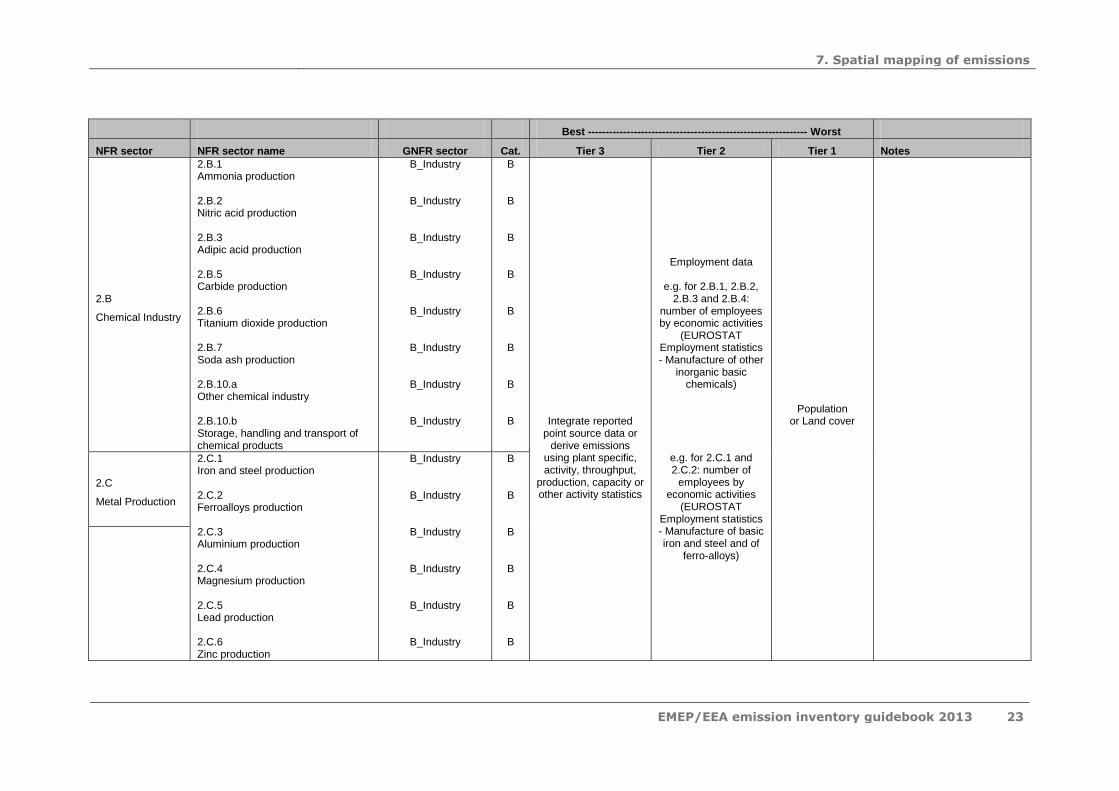
2.B
Chemical Industry
2.B.1 Ammonia production 2.B.2 Nitric acid production 2.B.3 Adipic acid production 2.B.5 Carbide production 2.B.6 Titanium dioxide production 2.B.7 Soda ash production 2.B.10.a Other chemical industry 2.B.10.b Storage, handling and transport of chemical products
B_Industry
B_Industry
B_Industry
B_Industry
B_Industry
B_Industry
B_Industry
B_Industry
B
B
B
B
B
B
B
B
Integrate reported point source data or
derive emissions using plant specific, activity, throughput,
production, capacity or other activity statistics
Employment data
e.g. for 2.B.1, 2.B.2, 2.B.3 and 2.B.4:
number of employees by economic activities
(EUROSTAT Employment statistics - Manufacture of other
inorganic basic chemicals)
e.g. for 2.C.1 and 2.C.2: number of
employees by economic activities
(EUROSTAT Employment statistics - Manufacture of basic iron and steel and of
ferro-alloys)
Population or Land cover
2.C
Metal Production
2.C.1 Iron and steel production 2.C.2 Ferroalloys production 2.C.3 Aluminium production 2.C.4 Magnesium production 2.C.5 Lead production 2.C.6 Zinc production
B_Industry
B_Industry
B_Industry
B_Industry
B_Industry
B_Industry
B
B
B
B
B
B

7. Spatial mapping of emissions
EMEP/EEA emission inventory guidebook 2013 24
Best -------------------------------------------------------------- Worst
NFR sector NFR sector name GNFR sector Cat. Tier 3 Tier 2 Tier 1 Notes
2.C.7.a Copper production 2.C.7.b Nickel production 2.C.7.c Other metal production 2.C.7.d Storage, handling and transport of metal products
B_Industry
B_Industry
B_Industry
B_Industry
B
B
B
B
Integrate reported point source data or
derive emissions using plant specific, activity, throughput,
production, capacity or other activity statistics
Employment data
e.g.: number of employees by
economic activities (EUROSTAT
Population or Land cover
2.D – 2.L
Solvent use and
Other production
2D3a Decorative coating application 2D3b Industrial coating application 2D3c Other coating application 2D3d Asphalt roofing 2D3e Road paving with asphalt
E_Solvents
E_Solvents
E_Solvents
B_Industry
B_Industry
D
B
B
D
D
Integrate reported point source data or
derive emissions using plant-specific, activity, throughput,
production, capacity or other activity statistics
Employment or
appropriate population data
e.g. for number of
employees by economic activities (Employment for coating industries including metal
packaging, vehicle refinishing, rolling
mills, vehicle repair, wood coating, ... )
Land cover
For Tier 2 where processes are industrial and there is a good employment dataset, use this. For emissions that result from consumption of products in the home, use population

7. Spatial mapping of emissions
EMEP/EEA emission inventory guidebook 2013 25
Best -------------------------------------------------------------- Worst
NFR sector NFR sector name GNFR sector Cat. Tier 3 Tier 2 Tier 1 Notes
2.D – 2.L
Solvent use and
Other industrial
production
2D3f Degreasing 2D3g Dry cleaning 2D3h Domestic solvent use including fungicides 2D3i Chemical products 2D3j Printing 2D3k Other solvent use 2G Other product use 2H1 Pulp and paper industry 2H2 Food and beverages industry 2H3 Other industrial processes 2I Wood processing 2J Production of POPs 2K Consumption of POPs and heavy metals (e.g. electrical and scientific equipment) 2L Other production, consumption, storage, transportation or handling of bulk products
E_Solvents
E_Solvents
E_Solvents
E_Solvents
E_Solvents
E_Solvents
E_Solvents
B_Industry
B_Industry
B_Industry
B_Industry
B_Industry
B_Industry
B_Industry
B
D
D
B
B
D
B
B
B
B
B
B
D
D
Integrate reported point source data or
derive emissions using plant-specific, activity, throughput,
production, capacity or other activity statistics
Employment or appropriate
population data
e.g. for number of employees by
economic activities (Employment in newspaper and
magazine industry)
e.g. for 3.D.2 and 3.D.3: population
density
Land cover
For Tier 2 where processes are industrial and there is a good employment dataset, use this. For emissions that result from consumption of products in the home, use population

7. Spatial mapping of emissions
EMEP/EEA emission inventory guidebook 2013 26
Best -------------------------------------------------------------- Worst
NFR sector NFR sector name GNFR sector Cat. Tier 3 Tier 2 Tier 1 Notes
3.B.1.a Manure management - Dairy cattle 3.B.1.b Manure management - Non-dairy cattle 3.B.2 Manure management – Sheep 3.B.3 Manure management - Swine 3.B.4.a Manure management – Buffalo 3.B.4.f Manure management – Goats 3.B.4.g Manure management – Horses 3.B.4.i Manure management - Mules and asses 3.B.4.j Manure management – Poultry 3.B.4.n Manure management - Other animals
K_AgriLivestock
K_AgriLivestock
K_AgriLivestock
K_AgriLivestock
K_AgriLivestock
K_AgriLivestock
K_AgriLivestock
K_AgriLivestock
K_AgriLivestock
K_AgriLivestock
D
D
D
C
D
D
D
D
C
D
Reported emissions from regulated farms
or detailed spatial farm livestock survey
statistics
Reported emissions from regulated farms
or detailed spatial farm livestock survey
statistics
Employment statistics or land cover and
agricultural production statistics
or land cover and livestock statistics
Employment statistics or land cover and
agricultural production statistics
or land cover and livestock statistics
Land cover for arable land
Land cover for arable land
When using these statistics care should be taken to account for possible over allocations to head/offices or market employment in urban areas that will distort the pattern of emissions and allocate too many emissions to urban areas When using these statistics care should be taken to account for possible over allocations to head/offices or market employment in urban areas that will distort the pattern of emissions and allocate too many emissions to urban areas
3.D – 3.I
Other agriculture
3.D.a.1 Inorganic N-fertilizers (includes also urea application) 3.D.a.2.a Animal manure applied to soils 3.D.a.2.b Sewage sludge applied to soils
L_AgriOther
L_AgriOther
L_AgriOther
D
D
D
Reported emissions from regulated farms
Employment statistics or land cover and
Land cover for arable land
For Tier 3 survey statistics for crop production can be

7. Spatial mapping of emissions
EMEP/EEA emission inventory guidebook 2013 27
Best -------------------------------------------------------------- Worst
NFR sector NFR sector name GNFR sector Cat. Tier 3 Tier 2 Tier 1 Notes
3.D.a.2.c Other organic fertilisers applied to soils (including compost) 3.D.a.3 Urine and dung deposited by grazing animals 3.D.a.4 Crop residues applied to soils 3.D.b Indirect emissions from managed soils 3.D.c Farm-level agricultural operations including storage, handling and transport of agricultural products 3.D.d Off-farm storage, handling and transport of bulk agricultural products 3.D.e Cultivated crops 3.D.f Use of pesticides 3.F Field burning of agricultural residues 3.I Agriculture other
L_AgriOther
L_AgriOther
L_AgriOther
L_AgriOther
L_AgriOther
L_AgriOther
L_AgriOther
L_AgriOther
L_AgriOther
L_AgriOther
D
D
D
D
D
D
D
D
D
D
or detailed spatial farm crop/fertilizer use
survey statistics
Reported emissions from regulated farms
or detailed spatial farm crop/fertilizer use
survey statistics
agricultural production statistics
or land cover and livestock statistics
Employment statistics or land cover and
agricultural production statistics
or land cover and livestock statistics
Land cover for arable land
combined with fertilizer use/stubble burning rates to estimate weightings by crop type. Farm level data is often commercially sensitive and may need to be aggregated For Tier 3 survey statistics for crop production can be combined with fertilizer use/stubble burning rates to estimate weightings by crop type. Farm level data is often commercially sensitive and may need to be aggregated
5.A – 5B
Biological
treatment of
waste
5.A Biological treatment of waste - Solid waste disposal on land 5.B.1 Biological treatment of waste – Composting
J_Waste
J_Waste
D
D
Waste disposal to land statistics and landfill disposal records by
site
Composting records
Evenly distributed emissions over landfill
site locations
Population statistics weighted with discontinuous urban fabric land
cover
Most countries with regulated land disposal will have records of landfill sites in use. It may be more difficult to identify disused sites or sites that are not regulated

7. Spatial mapping of emissions
EMEP/EEA emission inventory guidebook 2013 28
Best -------------------------------------------------------------- Worst
NFR sector NFR sector name GNFR sector Cat. Tier 3 Tier 2 Tier 1 Notes
5.B.2 Biological treatment of waste - Anaerobic digestion at biogas facilities
J_Waste
D
5.C
Waste
incineration
5.C.1.a Municipal waste incineration 5.C.1.b Industrial waste incineration 5.C.1.c Clinical waste incineration 5.C.1.d Sewage sludge incineration 5.C.1.e Cremation 5.C.1.f Other waste incineration 5.C.2 Open burning of waste
J_Waste
J_Waste
J_Waste
J_Waste
J_Waste
J_Waste
J_Waste
A
A
D
D
D
D
D
Regulated process emissions by site
Emissions distributed over known sites
based on capacity or population
Employment data for the specific
industry or population/ farm
statistics for small scale burning
Incineration 6Ca–d is generally regulated or controlled. Regulators or trade associations will hold site location details and often records of activity. Small scale waste burning (6Ce) should be distributed using population or farm statistics depending on the dominant small scale burning sector
5.D
Waste-water
handling
5.D.1 Domestic wastewater handling 5.D.2 Industrial wastewater handling 5.D.3 Other wastewater handling
J_Waste
J_Waste
J_Waste
D
D
D
Regulated process information and data
on wastewater treatment plant
Employment statistics for wastewater
treatment location of plant and capacity or
some surrogate of capacity-based on population density
Population statistics
Many countries now regulate wastewater treatment plant. Locations should be well known and activity data/emissions available by site
6 Other
6.A Other (included in National Total for Entire Territory)
R_Other D
11 Biogenic emissions and forest fires
Detailed surveys of land use types and
burned area combined with (Ing 2007) factors
for emissions
National emissions distributed using land
cover data and burned area data from
NatAir
Basic land cover data

7. Spatial mapping of emissions
EMEP/EEA emission inventory guidebook 2013 29
3.3.4 Example
3.3.4.1 Gridding methodology of the emissions from road transport (NFR sector
1.A.3.b)
Several European countries (e.g. BE, NL or UK) apply country specific methods to grid
emissions from road transport. In this section, the methodology developed by Theloke et al.
(2009) is described, as it is general and widely applicable over the whole of Europe. However,
note that some information sources quoted in this section are only available commercially.
Sector description
The emissions from road transport arise from the combustion of fuels such as gasoline, diesel,
liquefied petroleum gas (LPG), and natural gas in internal combustion engines (EMEP/EEA,
2013). The sector road transport considers all on road transportations of passengers as well as
good from all vehicle classes driven by fuel combustion. This sector is considered as diffuse
(see Table 1, NFR sector 1.A.3.b), therefore, according to the scheme presented in Figure 3-1,
compilation of point source emissions is not relevant and consequently the national reported
emissions can be considered as diffuse emissions.
Exhaust emissions from road transport (non exhaust emissions are not considered here) are
reported according to the following NFR sector codes:
1.A.3.b.i Road Transport: Passenger cars;
1.A.3.b.ii Road Transport: Light duty vehicles;
1.A.3.b.iii Road Transport: Heavy duty vehicles;
1.A.3.b.iv Road Transport: Mopeds & Motorcycles.
The allocation of emissions distinguishes on-road activities on the following street types:
highways;
rural roads;
urban roads.
Furthermore, the vehicle types are distinguished by fuel type for each relevant NFR code:
passengers cars (LPG, diesel and gasoline)
light duty vehicles (diesel and gasoline)
heavy duty vehicles (diesel)
motor cycles (two and four-strokes, gasoline)
Emission input data
Emission data used for the gridding procedure are reported sectoral totals from the CLRTAP
NFR sectors 1.A.3.b.i, Passenger cars; 1.A.3.b.ii, Light duty vehicles; 1.A.3.b.iii, Heavy duty
vehicles; 1.A.3.b.iv, Mopeds & Motorcycles.
Additional preparation of the emission data sets is necessary to distinguish between different
road and vehicle types. The first intermediate calculation is the allocation of the emissions
reported to CLRTAP into different road classes (highway, rural and urban) based on the
TREMOVE model (TREMOVE, 2010). The results are road and vehicle class specific shares
for each pollutant and country.
The next step is to harmonize the road and vehicle classes with the road network from the
TRANSTOOLS model (TRANSTOOLS, 2010). The road classes (highway, rural and urban)
7. Spatial mapping of emissions
EMEP/EEA emission inventory guidebook 2013 30
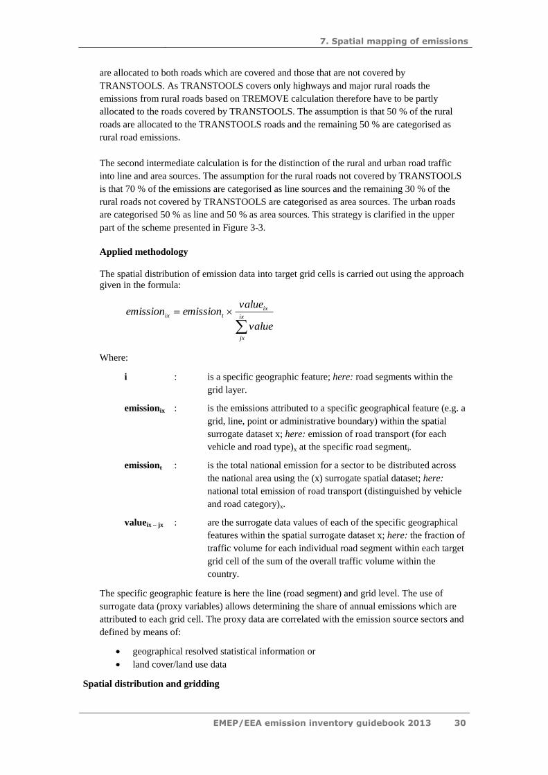
are allocated to both roads which are covered and those that are not covered by
TRANSTOOLS. As TRANSTOOLS covers only highways and major rural roads the
emissions from rural roads based on TREMOVE calculation therefore have to be partly
allocated to the roads covered by TRANSTOOLS. The assumption is that 50 % of the rural
roads are allocated to the TRANSTOOLS roads and the remaining 50 % are categorised as
rural road emissions.
The second intermediate calculation is for the distinction of the rural and urban road traffic
into line and area sources. The assumption for the rural roads not covered by TRANSTOOLS
is that 70 % of the emissions are categorised as line sources and the remaining 30 % of the
rural roads not covered by TRANSTOOLS are categorised as area sources. The urban roads
are categorised 50 % as line and 50 % as area sources. This strategy is clarified in the upper
part of the scheme presented in Figure 3-3.
Applied methodology
The spatial distribution of emission data into target grid cells is carried out using the approach
given in the formula:
ix
jx
ix
tix
value
valueemissionemission
Where:
i : is a specific geographic feature; here: road segments within the
grid layer.
emissionix : is the emissions attributed to a specific geographical feature (e.g. a
grid, line, point or administrative boundary) within the spatial
surrogate dataset x; here: emission of road transport (for each
vehicle and road type)x at the specific road segmenti.
emissiont : is the total national emission for a sector to be distributed across
the national area using the (x) surrogate spatial dataset; here:
national total emission of road transport (distinguished by vehicle
and road category)x.
valueix – jx : are the surrogate data values of each of the specific geographical
features within the spatial surrogate dataset x; here: the fraction of
traffic volume for each individual road segment within each target
grid cell of the sum of the overall traffic volume within the
country.
The specific geographic feature is here the line (road segment) and grid level. The use of
surrogate data (proxy variables) allows determining the share of annual emissions which are
attributed to each grid cell. The proxy data are correlated with the emission source sectors and
defined by means of:
geographical resolved statistical information or
land cover/land use data
Spatial distribution and gridding

7. Spatial mapping of emissions
EMEP/EEA emission inventory guidebook 2013 31
The methodology of the spatial distribution of the road transport can be summarised into the
following main steps:
1. Regionalisation of national emission releases: allocation of the emission values based
on traffic volume data for each road segment and also population density related to roads
not covered by TRANSTOOLS. This allocates the share of the national totals of each
specific pollutant to each road segment in the TRANSTOOLS model and to NUTS level
3 regions for the urban and rural traffic not covered by TRANSTOOLS.
2. Gridding: spatial distribution of the regionalised emission values on grid cell level is
based on TRANSTOOLS, GISCO (ROAD) (GISCO, 2010) road network and gridded
population density from JRC (Gallego, 2010). The result are gridded emissions for each
road segment and regional unit to each grid cell, using the following underlying
parameters:
Traffic volume and road network from TRANSTOOLS for highways and partly
for rural roads;
Road network divided by road type from GISCO (ROAD) for the roads not
covered in TRANSTOOLS (secondary and local roads);
Gridded population density as weighting factor for line sources in relation to
rural and urban roads not covered by TRANSTOOLS. Additionally as
distribution parameter for rural and urban area sources.
Degree of urbanisation (GISCO, 2010) for the categorization of the roads from
GISCO and the gridded population from JRC (Gallego, 2010) into urban and
rural.
The methodology for the spatial distribution of national total emissions from road transport
activities to a grid for each vehicle and road type is shown in Figure 3-3.
Figure 3-3 Overview of the applied methodology for the spatial distribution of the road
transport, Theloke et al. (2009).

7. Spatial mapping of emissions
EMEP/EEA emission inventory guidebook 2013 32
3.3.4.2 Gridding methodology for the diffuse emissions from Stationary
Combustion in Manufacturing Industries and Construction: Iron and Steel
(NFR sector 1.A.2.a)
Several European countries (e.g. BE, NL and UK) apply country specific methods to grid
diffuse emissions from industrial releases. In this paragraph, a general methodology based on
employment data is described. NFR sector 1.A.2.a is chosen as an example, but the
methodology can be applied for several sectors (see Table 1) and moreover is widely
applicable over the whole of Europe.
Sector description
The NFR sector 1.A.2.a, ‘Stationary Combustion in Manufacturing Industries and
Construction: Iron and Steel’, is dominated by E-PRTR related point sources, but is also
containing diffuse emissions (see Table 1). This comprises industrial releases from industrial
facilities not covered by the E-PRTR Regulation and its Annexes..
In this section, a methodology to spatially allocate the diffuse emissions from stationary
combustion in iron and steel industry is described.
Emission input data
As input emission data for the spatial distribution of diffuse industrial releases, national data
reported to the LRTAP Convention can be taken. To obtain the diffuse part of the country
specific emissions, not covered by the E-PRTR regulation, a subtraction methodology, as
described in 3.2, first needs to be applied.
Applied methodology
Diffuse industrial releases can be spatially distributed according to different proxy data. The
basic principle of distributing emissions is presented in the formula below using a surrogate
spatial dataset:
ix
jx
ix
tix
value
valueemissionemission
Where
i : is a specific geographic feature; here: a high resolution (e.g. 3 km
x 3 km) grid cell.
emissionix : is the emissions attributed to a specific geographical feature (e.g. a
grid, line, point or administrative boundary) within the spatial
surrogate dataset x; here: emission value attributed to each grid
cell.
emissiont : is the total national emission for a sector to be distributed across
the national area using the (x) surrogate spatial dataset; here:
when starting from the CLRTAP data, the diffuse industrial
emissions within a member state (subtraction methodology
required).

7. Spatial mapping of emissions
EMEP/EEA emission inventory guidebook 2013 33
valueix – jx : are the surrogate data values of each of the specific geographical
features within the spatial surrogate dataset x; here: a spatial
surrogate based on
number of employees according to the activity (e.g.
EUROSTAT Employment statistics - Manufacture of basic
iron and steel and of ferroalloys) and
"Industrial or Commercial units" from CORINE land cover
class (CLC2000/2006, 2010).
Thus, a combination of land use and employment statistics: the
share of employees in each ‘Industrial or Commercial’ CORINE
land cover unit, related to the national total of the employees.
The use of surrogate data (proxy variables) allows determining the share of annual emissions
that have to be attributed to each cell. The crucial part in the methodology described above, is
the construction of the spatial surrogate. It basically consists of the following steps:
Select the appropriate land cover types in the CORINE land cover map. Here:
"Industrial or commercial units" (CLC2000/2006, 2010);
Calculate the share of employees in each polygon of the selected units;
Use the employee weighted industrial zones as spatial surrogate in the above formula.
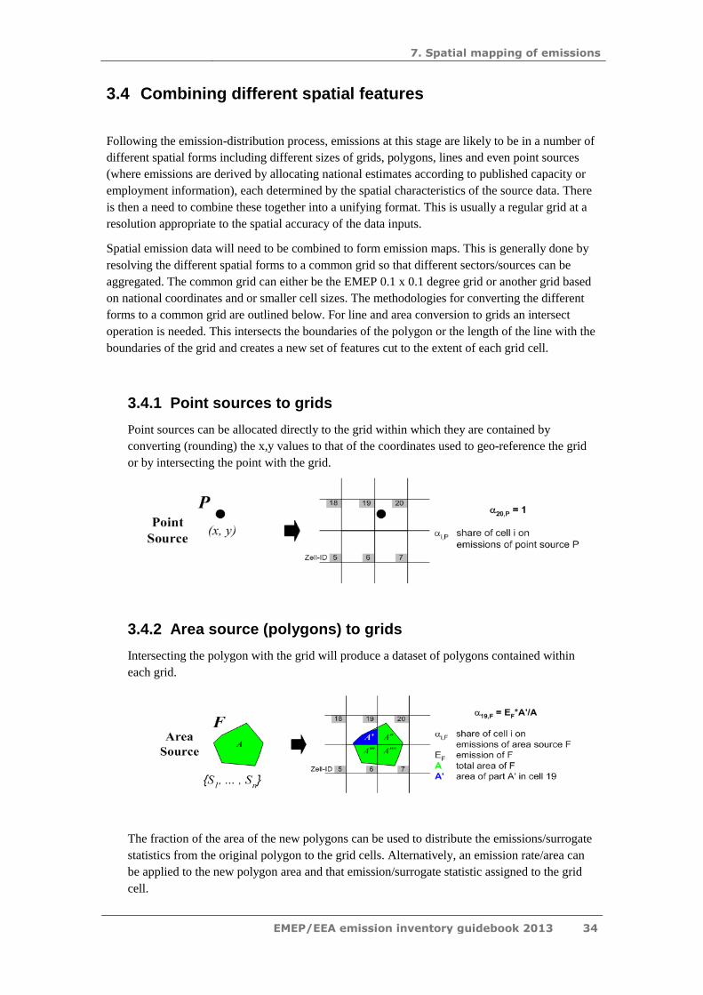
7. Spatial mapping of emissions
EMEP/EEA emission inventory guidebook 2013 34
3.4 Combining different spatial features
Following the emission-distribution process, emissions at this stage are likely to be in a number of
different spatial forms including different sizes of grids, polygons, lines and even point sources
(where emissions are derived by allocating national estimates according to published capacity or
employment information), each determined by the spatial characteristics of the source data. There
is then a need to combine these together into a unifying format. This is usually a regular grid at a
resolution appropriate to the spatial accuracy of the data inputs.
Spatial emission data will need to be combined to form emission maps. This is generally done by
resolving the different spatial forms to a common grid so that different sectors/sources can be
aggregated. The common grid can either be the EMEP 0.1 x 0.1 degree grid or another grid based
on national coordinates and or smaller cell sizes. The methodologies for converting the different
forms to a common grid are outlined below. For line and area conversion to grids an intersect
operation is needed. This intersects the boundaries of the polygon or the length of the line with the
boundaries of the grid and creates a new set of features cut to the extent of each grid cell.
3.4.1 Point sources to grids
Point sources can be allocated directly to the grid within which they are contained by
converting (rounding) the x,y values to that of the coordinates used to geo-reference the grid
or by intersecting the point with the grid.
3.4.2 Area source (polygons) to grids
Intersecting the polygon with the grid will produce a dataset of polygons contained within
each grid.
The fraction of the area of the new polygons can be used to distribute the emissions/surrogate
statistics from the original polygon to the grid cells. Alternatively, an emission rate/area can
be applied to the new polygon area and that emission/surrogate statistic assigned to the grid
cell.

7. Spatial mapping of emissions
EMEP/EEA emission inventory guidebook 2013 35
3.4.3 Line sources to grids
Intersecting the line features with the grid will produce a dataset of shorter line lengths
contained within each grid.
The fraction of the original line length of the new line can be used to distribute the
emissions/surrogate statistics from the original line to the grid cells. Alternatively, an
emission rate/unit of length can be applied to the new line length and that emission/surrogate
statistic assigned to the grid cell.
3.4.4 Converting between different spatial projections (e.g. GIS to EMEP)
In a number of cases, an inventory compiler may need to combine data from different spatial
datasets and extents to eventually derive the 0.1 x 0.1 degree EMEP grid.
The Open Geospatial Consortium Inc. provides guidance and standards for coordinate
transformation (see www.opengeospatial.org/standards/ct).
3.4.5 Aggregating to the UNECE GNFR
The aggregated sectors ‘gridded NFR’ (GNFR) for reporting are defined in Annex I to the
Guidelines for reporting emission data under the Convention on Long-range Transboundary
Air Pollution (1). These aggregations can be achieved through the aggregation of the spatially
resolved (mapped) detailed NFR sectors (or sector groups). Aggregation of NFR to GNFR
prior to mapping is not recommended as it may result in reduced accuracy in the placement of
emissions.

7. Spatial mapping of emissions
EMEP/EEA emission inventory guidebook 2013 36
4 Finding key spatial data sources
There are a number of different sources of spatial data. The first place to look should be national
statistical centres such as demographic, economic, transport, regulatory, energy, regulating bodies
and trade associations, as these data are likely to be most up-to-date.
4.1 General
4.1.1 Administrative boundaries
Statistics may be collected and stored with reference to regional or local government names
while the information that defines the spatial boundaries of these areas (geographies) could be
maintained in separate mapping datasets. Often a national mapping body is responsible for the
boundary datasets while specific statistics attributable to these boundaries can be available
from elsewhere. In these cases the statistics will need to be joined to the boundary dataset
using lookups between the statistical dataset and the spatial structure dataset (e.g. area IDs or
names). A number of common national datasets are listed below and give a starting point for
data collection activities.
4.1.2 Geo-referenced data
Some data will be available with grid reference attributes, whereas other data may have postal
address details. A grid reference lookup will be required to place the latter on a map.
Where national data is unavailable or too time consuming to collect, a number of international
datasets can be used (see section 4.3 of the present chapter).
4.2 National datasets
4.2.1 Population and employment
Most countries will have spatial population and employment datasets based on administrative
boundaries that can be used/combined to derive specific distributions or used as general
default distributions where other methods are not feasible. This is a good basic dataset that
can be used in many ways for distributing emissions from different sources.
4.2.2 Gas distribution networks
Information on gas supply by region or on a GIS basis is often available from energy
departments, from gas suppliers or from national statistical centres. Even national information
on the number of households with/without gas supply can be useful when combined with
population to estimate a distribution network.
4.2.3 Agricultural data
Most countries have agricultural census or survey data collected (e.g. livestock numbers, crop
production, fertilizer use) at a detailed spatial scale at administrative boundary level.

7. Spatial mapping of emissions
EMEP/EEA emission inventory guidebook 2013 37
4.2.4 Road network information
It is likely that many countries will hold national or commercial road network datasets that
includes the road geography. These can be used to help distribute road traffic emissions in
combination with traffic intensity statistics for administrative boundaries or specific count
points.
4.2.5 Rail
Rail networks can be relatively easy to identify and datasets of the network are usually held
by national mapping departments or organisations. Rail activity data is more difficult to obtain
but can be part of national statistics or generated from detailed timetable information.
4.2.6 Airport activity data
Many countries have detailed aircraft movement datasets as part of their national statistics.
These can be used to distribute emissions from Landing and Take-Off (LTO) and from airside
support vehicles to airport areas.
4.2.7 Aviation
National aviation authorities will have detailed databases of aircraft movements, the aircraft
type, origin and destination by airport. These data can be used to distribute the nationally
estimated emissions for Landing and Take-Off for domestic and international aviation and
allocate these emissions to the appropriate grid square.
4.2.8 National shipping
National shipping data is usually in the form of port arrival and departure statistics and
available from the national statistical authority. These will need to separate national and
international shipping but can be used to provide an indication of port activity for attributing
national emissions.
4.2.9 Point source information
Regulation of large point sources is common in most countries and public reporting of
regulated emissions occurs under the requirements of the Aarhus Convention PRTR Protocol,
LCPD and E-PRTR, all of which have established a requirement for regular point source
emissions reporting. Regulators within countries that are parties to these protocols and
directives will have publicly available records of reported emissions data. Alternative large
point source information sources can include:
trade associations
operators
statistical energy and productivity publications (capacity).
4.2.10 Local inventory data
In some cases local inventory data can be used to improve the spatial distribution of emissions
for transport and stationary sources by providing smaller process emissions by point source
and traffic information. However, integration of this data with the nationally reported data and
resolving emissions allocated to other areas can be time consuming and difficult to document.

7. Spatial mapping of emissions
EMEP/EEA emission inventory guidebook 2013 38
4.3 International datasets
There are a number of different international datasets that can be used to help derive the spatial
emissions of a country. In this section both publically and commercially available spatial data sets
are listed. It is mentioned if a data access fee is required.
Note that existing spatial emission inventories at international or European level can be used as
proxy data (or as such) to derive spatial emissions of a country. Existing spatial inventories are
however not listed here, an overview of spatial inventories is provided in section 5.
4.3.1 INSPIRE
In the future the EU intends to provide access to spatial datasets through the INSPIRE
programme http://inspire.jrc.ec.europa.eu/. A number of different geographical datasets will
be available under this European initiative.
4.3.2 CORINE land cover
If relevant national spatial statistics are not available then a simpler and less accurate method
using land cover data can be used to derive emissions.
The CORINE dataset provides processed satellite images showing different land cover
classes. This data can be accessed from: http://www.eea.europa.eu/data-and-maps/data/corine-
land-cover-2006-raster-2. Among the 43 different land covers provided, CORINE provides
the following datasets of relevance to emissions mapping:
continuous urban fabric
discontinuous urban fabric
industrial or commercial units
road and rail networks and associated land
port areas
airports
mineral extraction sites
dump sites
construction sites
green urban areas
arable land
sport and leisure facilities.
A number of these CORINE datasets can be used individually or in combination to generate
spatial distributions for sectoral emissions.
The IMPRESAREO project (Dore et al., 2001, 2004) derived weightings to apply to elements
of the CORINE land cover map to represent NFR sectors. These weightings are listed in the
table below.

7. Spatial mapping of emissions
EMEP/EEA emission inventory guidebook 2013 39
NFR Sector Land cover class Weighting
1.A.1, 1.A.2, 2 and 3 Industry 76 %
Continuous urban fabric 15 %
Discontinuous urban fabric 1 %
Ports 4 %
Airports 4 %
1.A.3.d.ii Ports 100 %
1.A.3.a.ii.(i) Airports 100 %
1.A.4.a Continuous urban fabric 50 %
Discontinuous urban fabric 50 %
4 Arable land 100 %
6.A Discontinuous urban fabric 100 %
Where CORINE or similar data is not available, satellite-based land cover data can often be
derived from raw images using the CORINE methodology.
4.3.3 ESA GlobCover
GlobCover is an ESA initiative which began in 2005 in partnership with JRC, EEA, FAO,
UNEP, GOFC-GOLD and IGBP. The aim of the project was to develop a service capable of
delivering global composites and land cover maps using as input observations from the 300m
MERIS sensor on board the ENVISAT satellite mission.
ESA makes available the land cover maps, which cover 2 periods: December 2004 - June
2006 and January - December 2009.
See: http://due.esrin.esa.int/globcover/
4.3.4 CORINE population
If relevant national spatial statistics are not available then for some sectors (see Table 1) a
simpler and less accurate method using population density data can be used to derive
emissions.
The CORINE population density dataset provides population density derived from the
CORINE 2000 land cover data set.
This data can be accessed from: http://www.eea.europa.eu/data-and-maps/data/population-
density-disaggregated-with-corine-land-cover-2000-2
4.3.5 SEDAC population
Where CORINE or similar data is not available, global population density data can be used.
The Socioeconomic Data and Applications Center (SEDAC) of NASA provides Gridded
Population of the World (GPW). GPWv3 depicts the distribution of human population across
7. Spatial mapping of emissions
EMEP/EEA emission inventory guidebook 2013 40
the globe. GPWv3 provides globally consistent and spatially explicit human population
information and data for use in research, policy making, and communications.
Population data estimates are provided for 1990, 1995, and 2000, and projected (in 2004,
when GPWv3 was released) to 2005, 2010, and 2015. The projected grids were produced in
collaboration with the United Nations Food and Agriculture Programme (FAO) as Population
Count and Density Grid Future Estimates. There is also an extensive map collection that
includes population density and sub-national administrative boundary maps (depicting the
input units) at country, continental, and global levels.
This data can be accessed from: http://sedac.ciesin.columbia.edu/data/collection/gpw-v3
4.3.6 Eurostat
Eurostat is a Directorate-General of the European Commission located in Luxembourg. Its
main responsibilities are to provide statistical information to the institutions of the European
Union (EU) and to promote the harmonisation of statistical methods across its member states
and candidates for accession as well as EFTA countries.
Employment data is available from Eurostat at NUTS 3 level, split into three categories:
services, industry and agriculture. Employment statistics are reported using the NACE
classification system.
Eurostat also has several useful datasets on ‘Industry, trade and services’, ‘Agriculture and
Fisheries’, and ‘Transport’.
This data can be accessed from:
http://epp.eurostat.ec.europa.eu/portal/page/portal/eurostat/home
4.3.7 ESRI data
ESRI provides a full spectrum of ready-to-use, high-quality geospatial data for your GIS
visualization and analysis projects. Some data sets are publically available and can be used for
spatial distribution of emissions. Interesting examples are locations of airports at global scale
(World Airports), World Roads, World Railroads, World Urban Areas, Europe Population
Density, ...
Data can be accessed from:
http://www.arcgis.com/home/group.html?owner=esri&title=ESRI%20Data%20%26%20Maps
&content=all
Some data sets are only commercially available, e.g. through ArcGIS licence. An example:
European rail network (included in ArcGIS version 9 installation CD-rom, (Railroads, ESRI
Data and Maps, ArcGIS 9).
4.3.8 Open Street Maps
OpenStreetMap (OSM) is a collaborative project to create a free editable map of the world.
Rather than the map itself, the data generated by the OpenStreetMap project is considered its
primary output. Examples of data made available through OSM are locations of airports, road
network, railroad network, …

7. Spatial mapping of emissions
EMEP/EEA emission inventory guidebook 2013 41
Geofabrik is a consulting and software development firm based in Karlsruhe, Germany
specializing in OSM services. The OSM data can easily be accessed through the Geofabrik
website: http://download.geofabrik.de/osm/europe/.
4.3.9 MapCruzin
Examples of data made available through MapCruzin are locations of airports, road network,
railroad network, waterways, …
This data can be accessed from: http://www.mapcruzin.com/free-europe-arcgis-maps-
shapefiles.htm
4.3.10 ICAO and EUROCONTROL
Airport statistics for major airports can be obtained from the International Civil Aviation
Organisation (ICAO) website if country-specific data are not available. See
www.icaodata.com/Trial/WhatIsICAO.aspx. Another interesting point of contact with respect
to airport statistics is EUROCONTROL (http://www.eurocontrol.int/).
Airport statistics can be used to distribute nationally calculated emissions to different airports
to estimate LTO emissions for each.
4.3.11 Shipping: Lloyds Register
The Lloyds Register contains detailed ship movements data that can be used to distribute
emissions from shipping. A fee is required to access the data.
See: http://www.lr.org/
4.3.12 COPERNICUS
COPERNICUS, the European Earth Observation programme, (previously called GMES) will
provide, accurate, timely and easily accessible information to improve the management of the
environment, understand and mitigate the effects of climate change and ensure civil security.
See http://copernicus.eu/

7. Spatial mapping of emissions
EMEP/EEA emission inventory guidebook 2013 42
5 Overview of available spatial emissions data
Table 2: Overview of available spatial emissions data. For each emission inventory the following information is provided: (i) Last and foreseen update, (ii) Sectoral,
spatial, and temporal resolution, (iii) Spatial and temporal coverage, (iv) Underlying emission and proxy data, (v) Developer. The gridding methodology is
discussed in a separate paragraph per inventory
Inventory Last
update
Foreseen
update
Sectoral
resolution
Spatial
resolution
Temporal
resolution
Spatial
coverage
Temporal
coverage
Underlying
emission data Reference Developer Data access
EDGAR 4.2 2011 Every 5 yrs IPCC sectors - 0.1 x 0.1 °
- per country Annual Global 1970-2008
calculation of
emissions using a
technology based
emission factor
approach
http://edgar.jrc.ec.europa.eu/in
dex.php
JRC
Publicly
available
Link to data
download
TNO-
MACC 2007 2012
SNAP01
sectors
0.125°
x 0.0625° Annual
Europe
(EU+ non-
EU)
2003-2007
(update to
incl. 2008-
2009)
Emissions reported
by European
Member States +
gapfilling using
IIASA and TNO
data
Kuenen et al. (2011) TNO
Available
on request
–
fee may be
required
E-PRTR
diffuse
emissions
2011 Not known
yet
NFR_09 and
CRF sector
5 x 5 km²
1 x 1 km² on
request
(EEA)
Annual
Europe
(EU27 and
EFTA
countries)
2008
Emissions reported
by European
Member States
Theloke et al. (2009) University
of Stuttgart
Publicly
available
Link to data
download
E-MAP 2012 Both spatial
distribution SNAP sectors
1 x 1 km²
Belgium; 5 x Annual Europe 1990-2009
Emissions reported
by European Maes et al. (2004)
Available
on request

7. Spatial mapping of emissions
EMEP/EEA emission inventory guidebook 2013 43
and national
totals:
yearly
5 km² Central
Europe; 60 x
60 km²
Europe
Member States –
fee may be
required
Other ???

7. Spatial mapping of emissions
EMEP/EEA emission inventory guidebook 2013 44
6 References
CEIP, 2010 – Technical Report CEIP 1/2010, Inventory Review 2010, Review of emission data reported under the LRTAP Convention and NEC Directive, Stage 1 and 2 review -
Status of gridded data and LPS data.
CLC2000, 2010 – EEA: CORINE Land Cover 2000 100 m (CLC2000)
CLC2006, 2010 – EEA: CORINE Land Cover 2006 100 m (CLC2006)
Dore et al., 2001 – IMPRESAREO - Improving the Spatial Resolution of Air Emission Inventories Using Earth Observation Data, WP 5000: Development of the Method for More
General Application to Urban Air Quality Issues; WP6000: Evaluation, Validation and
Refinement of Spatially Resolved Inventories for a Range of Urban Pollutants.
AEAT/ENV/R/0462, Culham.
Dore et al., 2004 – APMOSHERE, Air Pollution Modelling for Support to Policy on Health and
Environmental Risk in Europe (EVK2-2002-00577)). Emission Mapping Methodology Progress
Report (January 2004). AEA Technology, Netcen, UK
EMEP/EEA 2013, ‘1.A.3.b Exhaust emissions from road transport’ in ‘EMEP/EEA Air Pollutant
Emission Inventory Guidebook, 2013’, European Environment Agency,
(www.eea.europa.eu/emep-eea-guidebook)
Entec UK, 2005 – European Commission Directorate General Environment Service Contract on
Ship Emissions: Assignment, Abatement and Market-based Instruments. Contract No:
070501/2004/383959/MAR/C1, Task 1 - Preliminary Assignment of Ship Emissions to European
Countries. Final Report August 2005. Entec UK Limited. p.19.
Gallego et al., 2010 – A population density grid of the European Union, Population and
Environment (2010), 31: 460-473.
GISCO, 2010 – Geographic Information System of the European Commission (EUROSTAT),
http://epp.eurostat.ec.europa.eu/portal/page/portal/gisco_Geographical_information_maps/introdu
ction, 2010.
Gkatzoflias et al., 2007 – COPERT 4 model (http://www.eea.europa.eu/publications/copert-4-
2014-estimating-emissions), European Topic Centre on Air and Climate Change (ETC-ACC).
Kuenen et al., 2011 – TNO report, TNO-060-UT-2011-00588, MACC European Emission
Inventory for the years 2003-2007.
Maes et al., 2009 – Atmospheric Environment 43 (2009) 1246-1254, Spatial surrogates for the
disaggregation of CORINAIR emission inventories.
Theloke et al., 2009 – Final Report Diffuse Air Emissions in E-PRTR, Methodology development
for the spatial distribution of the diffuse emissions in Europe.
TRANSTOOLS, 2010 – URL: http://energy.jrc.ec.europa.eu/transtools/index.html, 02.04.2013.
TREMOVE, 2010 – URL: http://www.tremove.org/documentation/index.htm, 02.04.2013.

7. Spatial mapping of emissions
EMEP/EEA emission inventory guidebook 2013 45
7 Point of enquiry Enquiries concerning this chapter should be directed to the co-chairs of the Task Force on
Emission Inventories and Projections (TFEIP). Please refer to the TFEIP website
(www.tfeip-secretariat.org/) for the contact details of the current co-chairs.