384

7 New Statistical Features

7.1 System Files

PRELIS and LISREL generate several system files through which they can communicate with each other. These system files are binary files. Some of these system files can be used directly by users. Here we present these system files and their uses.

7.1.1 The PRELIS System File

The majority of software packages make use of a data file format that is unique to that package. These files are usually stored in a binary format so that reading and writing data to the hard drive is as fast as possible. Examples of file formats are

• Microsoft Excel (*.xls) • SPSS for Windows (*.sav) • Minitab (*.mtw) • SAS for Windows 6.12 (*.sd2) • STATA (*.dta) • STATISTICA (*.sta) • SYSTAT (*.sys)

These data system files usually contain all the known information about a specific data set. LISREL for Windows can import any of the above and many more file formats and convert them to a *.psf file. The *.psf file is analogous to, for example, a *.sav file in the sense that one can retrieve 3 types of information from a PRELIS system file:

• General information:

This part of the *.psf file contains the number of cases in the data set, the number of variables, global missing value codes and the position (number) of the weight variable.

• Variable information:

The variable name (8 characters maximum), and variable type (for example, continuous or ordinal), and the variable missing value code. For an ordinal variable the following information is also stored: the number of categories, and

385

category labels (presently 4 characters maximum) or numeric values assigned to each category.

• Data information:

Data values are stored in the form of a rectangular matrix, where the columns denote the variables and the rows the cases. Data are stored in double precision to ensure accuracy of all numerical calculations. By opening a *.psf file, the main menu bar expands to include the Data, Transformation, Statistics, Graphs and Multilevel menus. Selecting any of the options from these menus will activate the corresponding dialog box. The File and View menus are also expanded. See Chapter 2 for more details. An important feature of LISREL 8.50 is the use of *.psf files as part of the LISREL or SIMPLIS syntax. In doing so, one does not have to specify variable names, missing value codes, or the number of cases. The folders msemex and missingex contain many examples to illustrate this new feature. When building LISREL or SIMPLIS syntax from a path diagram, it is sufficient to select an appropriate *.psf file from the Add/Read option in the Setup, Variables dialog box. For more information and examples, see Chapter 4.

7.1.2 The Data System File

A data system file, or a *.dsf for short, is created each time PRELIS is run. Its name is the same as the PRELIS syntax file but with the suffix *.dsf. The *.dsf contains all the information about the variables that LISREL needs in order to analyze the data, i.e., variable labels, sample size, means, standard deviations, covariance or correlation matrix, and the location of the asymptotic covariance matrix, if any. The *.dsf file can be read by LISREL directly instead of specifying variable names, sample size, means, standard deviations, covariance or correlation matrix, and the location of the asymptotic covariance matrix using separate commands in a LISREL or SIMPLIS syntax file. To specify a *.dsf in the SIMPLIS command language, write:

System file from File filename.DSF

This line replaces the following typical lines in a SIMPLIS syntax file (other variations are possible):

386

Observed Variables: A B C D E F Means from File filename Covariance Matrix from File filename Asymptotic Covariance Matrix from File filename Sample Size: 678

To specify a *.dsf in the LISREL command language, write: SY=filename.DSF

This replaces the following typical lines in a LISREL syntax file (other variations are possible): DA NI=k NO=n ME=filename CM=filename AC=filename

As the *.dsf is a binary file, it can be read much faster than the syntax file. To make optimal use of this, consider the following strategy, assuming the data consists of many variables, possibly several hundreds, and a very large sample. Use PRELIS to deal with all problems in the data, i.e., missing data, variable transformation, recoding, definition of new variables, etc., and compute means and the covariance matrix or correlation matrix, say, and the asymptotic covariance matrix, if needed. Specify the *.dsf file, select the variables for analysis and specify the model in a LISREL or SIMPLIS syntax file. Several different sets of variables may be analyzed in this way, each one being based on a small subset of the variables in the *.dsf. The point is that there is no need to go back to PRELIS to compute new summary statistics of each LISREL model. With the SIMPLIS command language, selection of variables is automatic in the sense that only the variables included in the model will be used. The use of the *.dsf is especially important in simulations, as these will go much faster. The *.dsf also facilitates the building of SIMPLIS or LISREL syntax by drawing a path diagram.

7.1.3 The Model System File

A model system file, or *.msf for short, is created each time a LISREL syntax file containing a path diagram request is run. Its name is the same as the LISREL syntax file but with the suffix *.msf. The *.msf contains all the information about the model that LISREL needs to produce a path diagram, i.e., type and form of each parameter,

387

parameter estimates, standard errors, t-values, modification indices, fit statistics, etc. Usually, users do not have a direct need for the *.msf. For a complete discussion of this topic, please see the LISREL 8: New Statistical Features Guide.

7.2 Multiple Imputation

Multivariate data sets, where missing values occur on more than one variable, are often encountered in practice. Listwise deletion may result in discarding a large proportion of the data, which in turn, tends to introduce bias. Researchers frequently use ad hoc methods of imputation to obtain a complete data set. The multiple imputation procedure implemented in LISREL 8.50 is described in detail in Schafer (1997) and uses the EM algorithm and the method of generating random draws from probability distributions via Markov chains. In what follows, it is assumed that data are missing at random and that the observed data have an underlying multivariate normal distribution.

7.2.1 Technical Details

EM algorithm: Suppose '

1 2( , ,..., )py y y=y is a vector of random variables with mean µ and covariance

matrix Σ and that 1 2, ,..., ny y y is a sample from y.

Step 1: (M-Step)

Start with an estimate of µ and Σ , for example the sample means and covariances _

y and S based on a subset of the data, which have no missing values. If each row of the data set contains a missing value, start with µ = 0 and Σ = I.

Step 2: (E-Step)

Calculate ( | ; , )imiss iobsE∧ ∧

y y µ Σ and ( | ; , )imiss iobsCov∧ ∧

y y µ Σ , i = 1, 2, …, N.

388

Use these values to obtain an update of µ and Σ (M-step) and repeat steps 1 and 2 until

11( , )kk

∧ ∧++µ Σ are essentially the same as ( , )kk

∧ ∧µ Σ .

Markov chain Monte Carlo (MCMC): In LISREL 8.50, the estimates of µ and Σ obtained from the EM-algorithm are used as initial parameters of the distributions used in Step 1 of the MCMC procedure.

Step 1: (P-Step) Simulate an estimate kµ of µ and an estimate kΣ of Σ from a multivariate normal and

an inverted Wishart distribution respectively.

Step 2: (I-Step) Simulate | , 1, 2,...,imiss iobs i N=y y from conditional normal distributions with parameters

based on kµ and kΣ .

Replace the missing values with simulated values and calculate _

1k+ =µ y and 1k+ =Σ S

where _

y and S are the sample means and covariances of the completed data set respectively. Repeat Steps 1 and 2 m times. In LISREL, missing values in row i are replaced by the average of the simulated values over the m draws, after an initial burn-in period. See Chapter 3 for a numerical example.

7.3 Full Information Maximum Likelihood (FIML) for Continuous Variables

Suppose that 1 2( , , , ) 'py y y=y � has a multivariate normal distribution with mean µ and

covariance matrix Σ and that 1 2, ,..., ny y y is a random sample of the vector y .

Specific elements of the vectors , 1, 2, ,k k n=y … may be unobserved so that the data set

comprising of n rows (the different cases) and p columns (variables 1, 2, . . . , p ) have missing values.

389

Let ky denote a vector with incomplete observations, then this vector can be replaced by *k k k=y X y where kX is a selection matrix, and ky has typical elements

1 2( , , , )k k kpy y y… with one or more of the skjy missing, 1, 2, , .j p= …

Example: Suppose 3p = , and that variable 2 is unobserved, then

11*

23

3

1 0 0.

0 0 1

kk

k kk

k

yy

yy

y

= =

y

From the above example it can easily be seen that kX is based on an identity matrix with

rows deleted according to missing elements of ky .

If an observed vector ky contains no unobserved values, then kX is equal to the identity

matrix and hence *k k=y y .

Without loss in generality, 1 2( , , )ny y y… can be replaced with * * *

1 2( , , )ny y y… where *ky ,

1, 2, ,k n= … has a normal distribution with mean kX µ and covariance matrix 'k kX ΣX .

The log-likelihood for the non-missing data is *

1

log ( , , )n

k k kk

f=

∑ y µ Σ , where *( , , )k k kf y µ Σ

is the pdf of k kX y given the parameters k k=µ X µ and 'k k k=Σ X ΣX .

In practice, when data are missing at random, there are usually M patterns of missingness, where M n< . When this is the case, the computational burden of evaluating n likelihood functions is considerably decreased. It is customary to define the chi-square statistic as 2

0 1F Fχ = − , where 0 02 lnF L= − ,

1 12 lnF L= − , and where 1ln L denotes the log-likelihood (at convergence) when no

restrictions are imposed on the parameters (µ and Σ ). The quantity 0ln L denotes the log-

likelihood value (at convergence) when parameters are restricted according to a postulated model. The degrees of freedom equals ν , where ( 1) / 2p p p kν = + + − and k is the number of parameters in the model. See the examples in Section 4.8. Additional examples are given in the missingex folder.

390

7.4 Multilevel Structural equation Modeling

7.4.1 Multilevel Structural equation Models

Social science research often entails the analysis of data with a hierarchical structure. A frequently cited example of multilevel data is a dataset containing measurements on children nested within schools, with schools nested within education departments. The need for statistical models that take account of the sampling scheme is well recognized and it has been shown that the analysis of survey data under the assumption of a simple random sampling scheme may give rise to misleading results. Iterative numerical procedures for the estimation of variance and covariance components for unbalanced designs were developed in the 1980s and were implemented in software packages such as MLWIN, SAS PROC MIXED and HLM. At the same time, interest in latent variables, that is, variables that cannot be directly observed or can only imperfectly be observed, led to the theory providing for the definition, fitting and testing of general models for linear structural relations for data from simple random samples. A more general model for multilevel structural relations, accommodating latent variables and the possibility of missing data at any level of the hierarchy and providing the combination of developments in these two fields, was a logical next step. In papers by Goldstein and MacDonald (1988), MacDonald and Goldstein (1989) and McDonald (1993), such a model was proposed. Muthén (1990, 1991) proposed a partial maximum likelihood solution as simplification in the case of an unbalanced design. An overview of the latter can be found in Hox (1993). General two-level structural equation modeling is available in LISREL 8.50. Full information maximum likelihood estimation is used, and a test for goodness of fit is given. An example, illustrating the implementation of the results for unbalanced designs with missing data at both levels of the hierarchy, is also given.

7.4.2 A General Two-level Structural equation Model

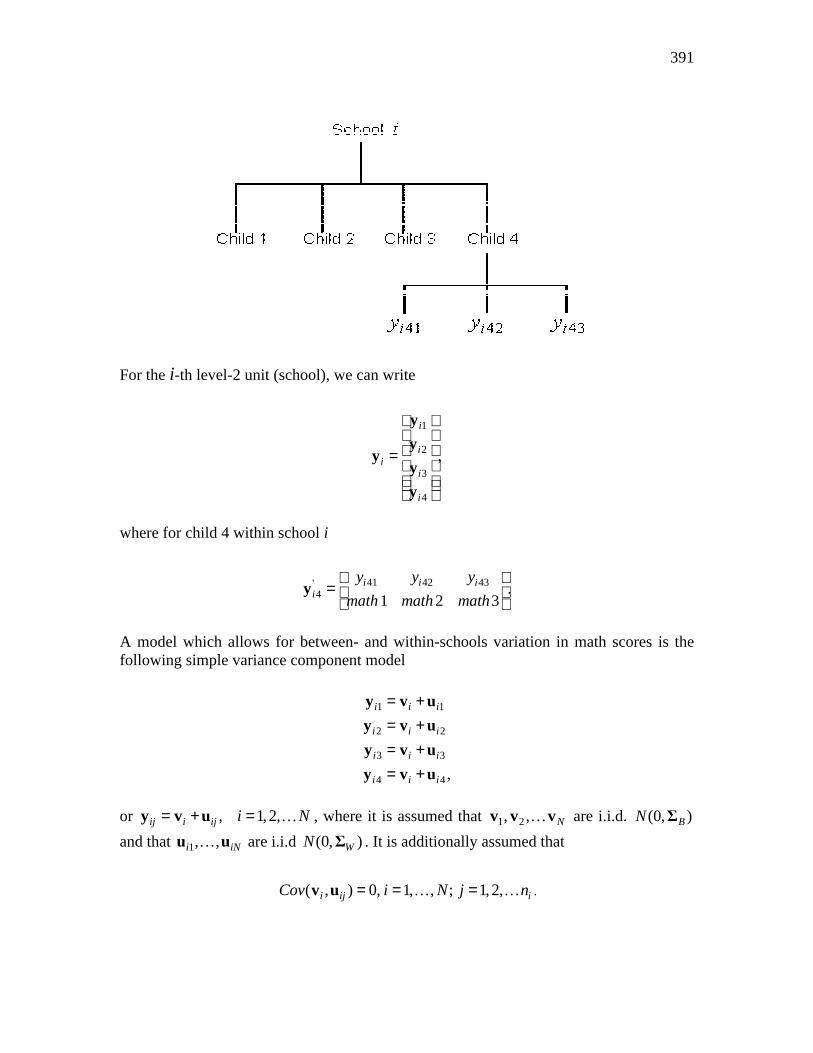
Consider a data set consisting of 3 measurements, math 1, math 2, and math 3, made on each of 1000 children who are nested within N = 100 schools. This data set can be schematically represented for school i as follows

391

For the i-th level-2 unit (school), we can write

1

2

3

4

,

i

ii

i

i

=

y

yy

y

y

where for child 4 within school i

41 42 43'

4 .1 2 3

i i ii

y y y

math math math

=

y

A model which allows for between- and within-schools variation in math scores is the following simple variance component model

1 1

2 2

3 3

4 4 ,

i i i

i i i

i i i

i i i

= += += += +

y v u

y v u

y v u

y v u

or , 1,2,ij i ij i N= + =y v u … , where it is assumed that 1 2, , Nv v v… are i.i.d. (0, )BN Σ

and that 1, ,i iNu u… are i.i.d (0, )WN Σ . It is additionally assumed that

( , ) 0, 1, , ; 1,2,i ij iCov i N j n= = =v u … … .

392

From the distributional assumptions it follows that

'( , )

B W B B B

B B W B Bi i

B B B W B

B B B B W

Cov

+ + = + +

Σ Σ Σ Σ Σ

Σ Σ Σ Σ Σy y

Σ Σ Σ Σ Σ

Σ Σ Σ Σ Σ

or ' '( , )i i B WCov = ⊗ + ⊗y y 11 Σ I Σ . It also follows that

( )iE =y 0 .

In practice, the latter assumption ( )iE =y 0 is seldom realistic, since measurements such

as math scores do not have zero means. One approach to this problem is to use grand mean centering. Alternatively, one can add a fixed component to the model ,ij i ij= +y v u

so that

,ij ij i ij= + +y X β v u (7.1)

where ijX denotes a design matrix and β a vector of regression coefficients.

Suppose that for the example above, the only measurements available for child 1 are math 1 and math 3 and for child 2 math 2 and math 3. Let 1iS and 2iS be selection matrices defined as follows

1

1 0 0,

0 0 1i

=

S therefore 11

3

ii i

i

v

v

=

S v

and

2

0 1 0,

0 0 1i

=

S therefore 22

3

.ii i

i

v

v

=

S v

In general, if p measurements were made, ijS (see, for example, du Toit, 1995) consists

of a subset of the rows of the p p× identity matrix pI , where the rows of ijS correspond

to the response measurements available for the (i, j)-th unit.

393

The above model can be generalized to accommodate incomplete data by the inclusion of these selection matrices. Hence

( )ij y ij ij i ij ij= + +y X β S v S u (7.2)

where ( )yX is a design matrix of the appropriate dimensions.

If we further suppose that we have a 1q× vector of variables ix characterizing the level-

2 units (schools), then we can write the observed data for the i-th level-2 unit as

' ' ' ' '1 2[ , ,..., , ],

ii i i in i=y y y y x

where

'1 2[ , ,..., ]ij ij ij ijpy y y=y

and

'

1 2[ , ,..., ].i i i iqx x x=x (7.3)

We assume that ijy and ix can be written as

( ) , 1,2,ij y ij y ij i ij ij ij n= + + =y X β S v S u … (7.4)

( ) , 1, 2,i x i x i i i Nβ= + =x X R w … (7.5)

where ( )yX and ( )xX are design matrices for fixed effects, and ijS and iR are selection

matrices for random effects of order ijp p× and iq q× respectively. Note that (7.4)

defines two types of random effects, where iv is common to level-3 units and iju is

common to level-1 units nested within a specific level-2 unit. Additional distributional assumptions are

( ) , 1, 2, ,

( , ) , 1, 2, , ; 1, 2, ,

( , ) .

i xx

ij i xy i

ij i

Cov i N

Cov i N j n

Cov

= == = =

=

w Σ

y w Σ

u w 0

�

� … (7.6)

394

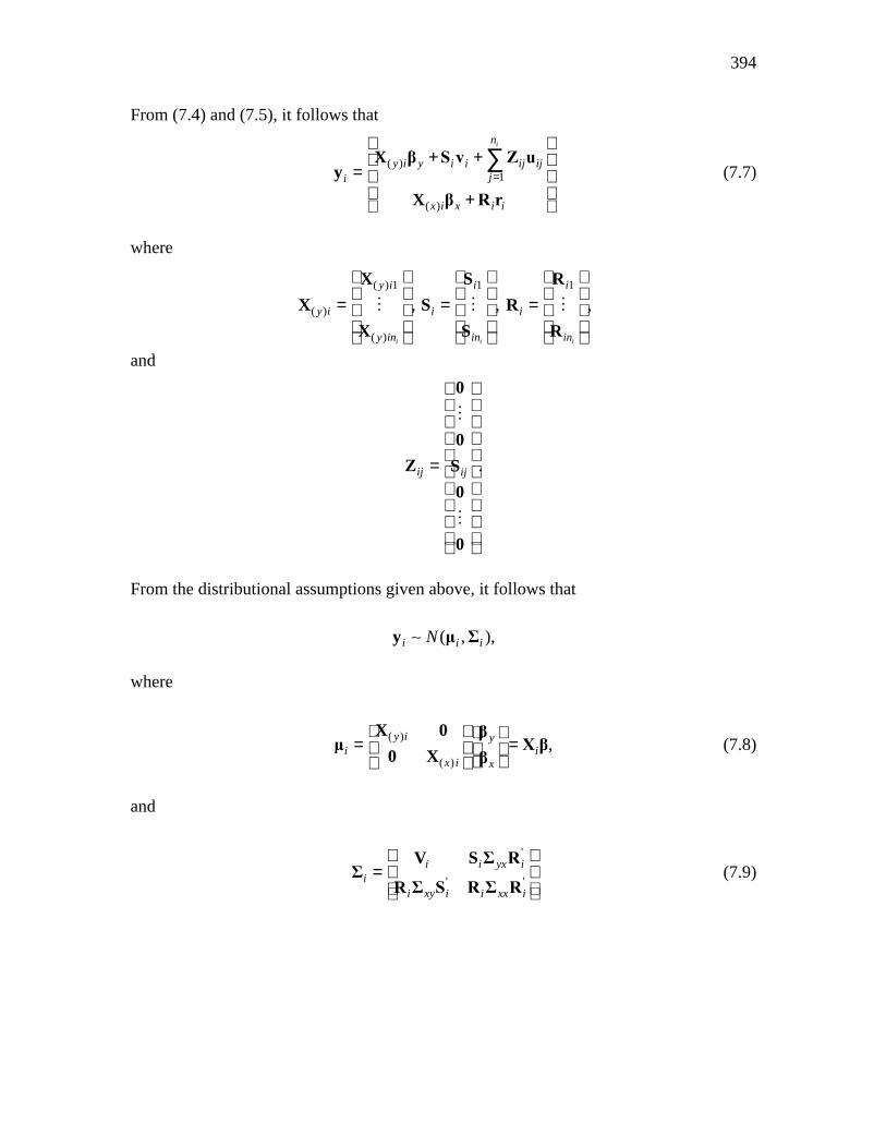
From (7.4) and (7.5), it follows that

( )

1

( )

in

y i y i i ij ijji

x i x i i

=

+ +

= +

∑X β S v Z uy

X β R r

(7.7)

where

( ) 1

( )

( ) i

y i

y i

y in

=

X

X

X

� ,1

i

i

i

in

=

S

S

S

� , 1

i

i

i

in

=

R

R

R

� ,

and

.ij ij

=

0

0

Z S

0

0

�

�

From the distributional assumptions given above, it follows that

( , ),i i iNy µ Σ∼

where

( )

( )

,y i y

i ix i x

= =

X 0 βµ X β

0 X β (7.8)

and

'

' '

i i yx ii

i xy i i xx i

=

V S Σ RΣ

R Σ S R Σ R (7.9)

395

where

1' '

1

.i

i

i n

i i B i ij W ijj

in

Cov=

= = +

∑y

V S Σ S Z Σ Z

y

�

Remark If i q=R I and ij p=S I , corresponding to the case of no missing y or x variables, then

'i yx i yx= ⊗S Σ R 1 Σ where '1 is a 1in × row vector (1,1, …,1).

Furthermore, for , 1, 2, ,ij p ij n= =S I …

'

ii n W B= ⊗ + ⊗V I Σ 11 Σ

(see, for example, MacDonald and Goldstein, 1989). The unknown parameters in (7.8) and (7.9) are β , BvecsΣ , WvecsΣ , xyvecsΣ and .xxvecsΣ

Structural models for the type of data described above may be defined by restricting the elements of β , BΣ , WΣ , xyΣ , and xxΣ to be some basic set of parameters

'1 2( , , , )kγ γ γ=γ … .

For example, assume the following pattern for the matrices WΣ and BΣ , where WΣ

refers to the within (level-1) covariance matrix and BΣ to the between (level-2) covariance matrix:

'

' .

W W W W W

B B B B B

= +

= +

Σ Λ Ψ Λ D

Σ Λ Ψ Λ D (7.10)

Factor analysis models typically have the covariance structures defined by (7.10). Consider a confirmatory factor analysis model with 2 factors and assume 6p = .

11

21

31

42

52

62

0

0

0

0

0

0

W

λλλ

λλλ

=

Λ , 11 12

21 22W

ψ ψψ ψ

=

Ψ ,

396

and

11

66

.WD

θ

θ

=

�

If we restrict all the parameters across the level-1 and level-2 units to be equal, then

'

11 21 44 11 21 22 11 66[ , , , , , , , , , ]λ λ λ ψ ψ ψ θ θ=γ … …

is the vector of unknown parameters.

7.4.3 Maximum Likelihood for General Means and Covariance Structures

In this section, we give a general framework for normal maximum likelihood estimation of the unknown parameters. In practice, the number of variables (p + q) and the number of level-1 units within a specific level-2 unit may be quite large, which leads to iΣ

matrices of very high order. It is therefore apparent that further simplification of the likelihood function derivatives and Hessian is required if the goal is to implement the theoretical results in a computer program. These aspects are addressed in du Toit and du Toit (forthcoming). Denote the expected value and covariance matrix of iy by iµ and iΣ respectively (see

(7.8) and (7.9)). The log-likelihood function of 1 2, , , Ny y y… may then be expressed as

1 '

1

1ln { ln 2 ln | | ( )( ) }

2

N

i i i i i ii

L n trπ −

== − + + − −∑ Σ Σ y µ y µ (7.11)

Instead of maximizing ln L , maximum likelihood estimates of the unknown parameters are obtained by minimizing ln L− with the constant term omitted, i.e., by minimizing the following function

1

1

1( ) {ln | | },

2 i

N

i i yi

F tr −

== +∑γ Σ Σ G (7.12)

where

'( )( ) .

iy i i i i= − −G y µ y µ (7.13)

397

Its minimum ( )F∂ =

∂γ

0γ

yields the normal maximum likelihood estimator ∧γ of the

unknown vector of parameters γ . Unless the model yields maximum likelihood estimators in closed form, it will be necessary to make use of an iterative procedure to minimize the discrepancy function. The optimization procedure (Browne and du Toit, 1992) is based on the so-called Fisher scoring algorithm, which in the case of structured means and covariances may be regarded as a sequence of Gauss-Newton steps with quantities to be fitted as well as the weight matrix changing at each step. Fisher scoring algorithms require the gradient vector and an approximation to the Hessian matrix.

7.4.4 Fit Statistics and Hypothesis Testing

The multilevel structural equation model, ( )M γ , and its assumptions imply a covariance

structure ( )BΣ γ , ( )WΣ γ , ( )xyΣ γ , ( )xxΣ γ and mean structure ( )µ γ for the observable

random variables where γ is a 1k × vector of parameters in the statistical model. It is

assumed that the empirical data are a random sample of N level-2 units and 1

Nii

n=∑

level-1 units, where in denotes the number of level-1 units within the i-th level-2 unit.

From this data, we can compute estimates of µ , BΣ , …, xxΣ if no restrictions are

imposed on their elements. The number of parameters for the unrestricted model is

* 1 1

2 ( 1) ( 1)2 2

k m p p pq q q = + + + + +

and is summarized in the * 1k × vector π . The unrestricted model ( )M π can be regarded as the “baseline” model. To test the model ( )M γ , we use the likelihood ratio test statistic

2ln ( ) 2 ln ( )c L L∧ ∧

= − −γ π (7.14)

If the model ( )M γ holds, c has a 2χ -distribution with *d k k= − degrees of freedom. If

the model does not hold, c has a non-central 2χ -distribution with d degrees of freedom and non-centrality parameter λ that may be estimated as (see Browne and Cudeck, 1993):

max{( ),0}c dλ∧

= − (7.15) These authors also show how to set up a confidence interval for λ .

398

It is possible that the researcher has specified a number of competing models

1 1 2 2( ), ( ), , ( ).k kM M Mγ γ γ… If the models are nested in the sense that : 1j jk ×γ is a

subset of : 1i ik ×γ , then one may use the likelihood ratio test with degrees of freedom

i jk k− to test ( )jM γ against ( )iM γ .

Another approach is to compare models on the basis of some criteria that take parsimony as well as fit into account. This approach can be used regardless of whether or not the models can be ordered in a nested sequence. Two strongly related criteria are the AIC measure of Akaike (1987) and the CAIC of Bozdogan (1987).

AIC 2c d= + (7.16)

1

CAIC (1 ln )N

ii

c n d=

= + + ∑ (7.17)

The use of c as a central 2χ -statistic is based on the assumption that the model holds exactly in the population. A consequence of this assumption is that models that hold approximately in the population will be rejected in large samples. Steiger (1990) proposed the root mean square error of approximation (RMSEA) statistic that takes particular account of the error of approximation in the population

0

,F

RMSEAd

∧

= (7.18)

where 0F∧

is a function of the sample size, degrees of freedom and the fit function. To use the RMSEA as a fit measure in multilevel SEM, we propose

0 max ,0c d

FN

∧ − = (7.19)

Browne and Cudeck (1993) suggest that an RMSEA value of 0.05 indicates a close fit and that values of up to 0.08 represent reasonable errors of approximation in the population.

7.4.5 Starting Values and Convergence Issues

In fitting a structural equation model to a hierarchical data set, one may encounter convergence problems unless good starting values are provided. A procedure that appears to work well in practice is to start the estimation procedure by fitting the unrestricted

399

model to the data. The first step is therefore to obtain estimates of the fixed components ( )β and the variance components ( , , and ).B xy xx WΣ Σ Σ Σ Our experience with the Gauss-

Newton algorithm (see, for example, Browne and du Toit, 1992) is that convergence is usually obtained within less than 15 iterations, using initial estimates

, , ,B p xy xx q= = = =β 0 Σ I Σ 0 Σ I and W p=Σ I . At convergence, the value of 2 ln L− is

computed.

Next, we treat

B yx

B

xy xx

∧ ∧

∧ ∧

=

Σ ΣS

Σ Σ

and WW

∧ Σ =

0S0 0

as sample covariance matrices and fit a two-group structural equation model to the between- and within-groups. Parameter estimates obtained in this manner are used as the elements of the initial parameter vector 0γ .

In the third step, the iterative procedure is restarted and kγ updated from 1k−γ , k = 1,2,…

until convergence is reached. The following example illustrates the steps outlined above. The data set used in this section forms part of the data library of the Multilevel Project at the University of London, and comes from the Junior School Project (Mortimore et al, 1988). Mathematics and language tests were administered in three consecutive years to more than 1000 students from 49 primary schools, which were randomly selected from primary schools maintained by the Inner London Education Authority.

The following variables were selected from the data file:

• School School code (1 to 49) • Math1 Score on mathematics test in year 1 (score 1 - 40) • Math2 Score on mathematics test in year 2 (score 1 - 40) • Math3 Score on mathematics test in year 3 (score 1 - 40)

The school number (School) is used as the level-2 identification.

400

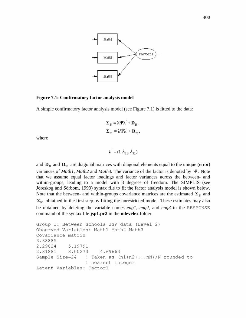
Figure 7.1: Confirmatory factor analysis model

A simple confirmatory factor analysis model (see Figure 7.1) is fitted to the data:

'

'

,

,

B B

W W

= +

= +

Σ λΨλ D

Σ λΨλ D

where

'

21 31(1, , )λ λ=λ

and BD and WD are diagonal matrices with diagonal elements equal to the unique (error)

variances of Math1, Math2 and Math3. The variance of the factor is denoted by Ψ . Note that we assume equal factor loadings and factor variances across the between- and within-groups, leading to a model with 3 degrees of freedom. The SIMPLIS (see Jöreskog and Sörbom, 1993) syntax file to fit the factor analysis model is shown below. Note that the between- and within-groups covariance matrices are the estimated BΣ and

WΣ obtained in the first step by fitting the unrestricted model. These estimates may also

be obtained by deleting the variable names eng1, eng2, and eng3 in the RESPONSE command of the syntax file jsp1.pr2 in the mlevelex folder. Group 1: Between Schools JSP data (Level 2) Observed Variables: Math1 Math2 Math3 Covariance matrix 3.38885 2.29824 5.19791 2.31881 3.00273 4.69663 Sample Size=24 ! Taken as (n1+n2+...nN)/N rounded to ! nearest integer Latent Variables: Factor1

401

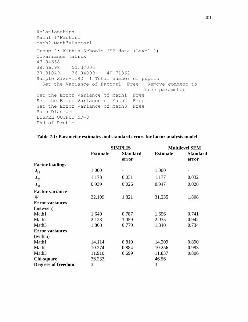
Relationships Math1=1*Factor1 Math2-Math3=Factor1

Group 2: Within Schools JSP data (Level 1) Covariance matrix 47.04658 38.56798 55.37006 30.81049 36.04099 40.71862 Sample Size=1192 ! Total number of pupils ! Set the Variance of Factor1 Free ! Remove comment to !free parameter Set the Error Variance of Math1 Free Set the Error Variance of Math2 Free Set the Error Variance of Math3 Free Path Diagram LISREL OUTPUT ND=3 End of Problem

Table 7.1: Parameter estimates and standard errors for factor analysis model

SIMPLIS Multilevel SEM Estimate Standard

error Estimate Standard

error Factor loadings

11λ 1.000 - 1.000 -

21λ 1.173 0.031 1.177 0.032

31λ 0.939 0.026 0.947 0.028

Factor variance Ψ 32.109 1.821 31.235 1.808 Error variances (between)

Math1 1.640 0.787 1.656 0.741 Math2 2.123 1.059 2.035 0.942 Math3 1.868 0.779 1.840 0.734 Error variances (within)

Math1 14.114 0.810 14.209 0.890 Math2 10.274 0.884 10.256 0.993 Math3 11.910 0.699 11.837 0.806 Chi-square 36.233 46.56 Degrees of freedom 3 3

402

Table 7.1 shows the parameter estimates, estimated standard errors and 2χ -statistic values obtained from the SIMPLIS output and from the multilevel SEM output respectively. Remarks:

1. The between-groups sample size of 26 used in the SIMPLIS syntax file was

computed as 1

1 Nii

nN =∑ , where N is the number of schools and in the number of

children within school i. Since this value is only used to obtain starting values, it is not really crucial how the between-group sample size is computed. See, for example, Muthén (1990,1991) for an alternative formula.

2. The within-group sample size of 1192 used in the SIMPLIS file syntax is equal to the total number of school children.

3. The number of missing values per variable is as follows: Math1: 38 Math2: 63 Math3: 239 The large percentage missing for the Math3 variable may partially explain the relatively large difference in 2χ -values from the SIMPLIS and multilevel SEM outputs.

4. If one allows for the factor variance parameter to be free over groups, the 2χ fit statistic becomes 1.087 at 2 degrees of freedom. The total number of multilevel SEM iterations required to obtain convergence equals eight.

In conclusion, a small number of variables and a single factor SEM model were used to illustrate the starting values procedure that we adopted. The next section contains additional examples, also based on a schools data set. Another example can be found in du Toit and du Toit (forthcoming). Also see the msemex folder for additional examples.

7.4.6 Practical Applications

The example discussed in this section is based on school data that were collected during a 1994 survey in South Africa. A brief description of the SA_Schools.psf data set in the msemex folder is as follows: N = 136 schools were selected and the total number of children within schools

16047

Nii

n=

=∑ , where in varies from 20 to 60. A description of the variables is given in

Table 7.2.

403

Table 7.2: Description of variables in SA_School.psf

Name Description Number missing

Pupil Level-1 identification 0 School Level-2 identification 0 Intcept All values equal to 1 0 Grade 0 = Grade 2

1 = Grade 3 2 = Grade 4

0

Language 0 = Black 1 = White

0

Gender 1 = Male 2 = Female

1

Mothedu Mother’s level of education on a scale from 1 to 7 783 Fathedu Father’s level of education on a scale from 1 to 7 851 Read Speech Write Arithm

Teacher’s evaluation on a scale from 1 to 5: 1 = Poor 5 = Excellent

482 470 467 451

Socio Socio-economic status indicator, scale 0 to 5 on school level

0

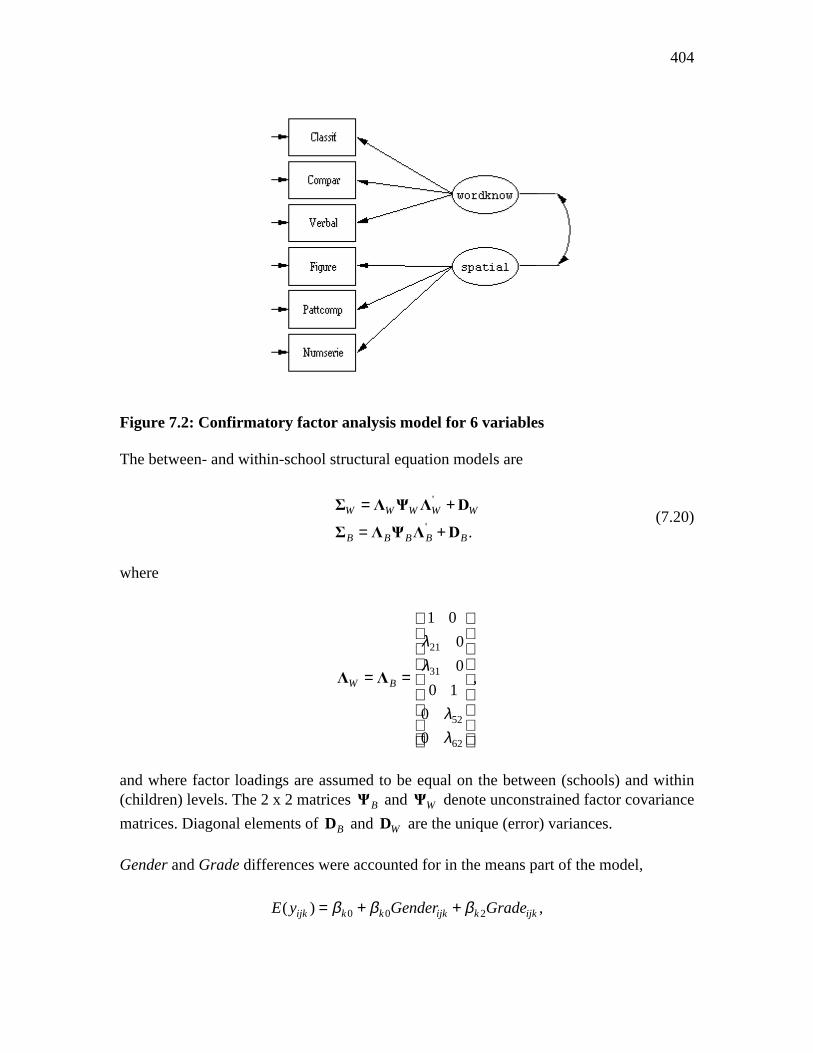
Classif Classification: total correct out of 30 items 23 Compar Comparison: total correct out of 23 items 27 Verbal Verbal Instructions: total correct out of 50 items 20 Figure Figure Series: total correct out of 24 items 118 Pattcomp Pattern Completion: total correct out of 24 items 109 Knowled Knowledge: total correct out of 32 items 112 Numserie Number Series: total correct out of 15 items 2305 The variables Language and Socio are school-level variables and their values do not vary within schools. Listwise deletion of missing cases results in a data set containing only 2691 of the original 6047 cases. For this example, we use the variables Classif, Compar, Verbal, Figure, Pattcomp and Numserie from the schools data set discussed in the previous section. Two common factors are hypothesized: word knowledge and spatial ability. The first three variables are assumed to measure wordknow and the last three to measure spatial. A path diagram of the hypothesized factor model is shown in Figure 7.2.

404

Figure 7.2: Confirmatory factor analysis model for 6 variables The between- and within-school structural equation models are

'

' .

W W W W W

B B B B B

= +

= +

Σ Λ Ψ Λ D

Σ Λ Ψ Λ D (7.20)

where

21

31

52

62

1 0

0

0,

0 1

0

0

W B

λλ

λλ

= =

Λ Λ

and where factor loadings are assumed to be equal on the between (schools) and within (children) levels. The 2 x 2 matrices BΨ and WΨ denote unconstrained factor covariance

matrices. Diagonal elements of BD and WD are the unique (error) variances.

Gender and Grade differences were accounted for in the means part of the model,

0 0 2( ) ,ijk k k ijk k ijkE y Gender Gradeβ β β= + +

405

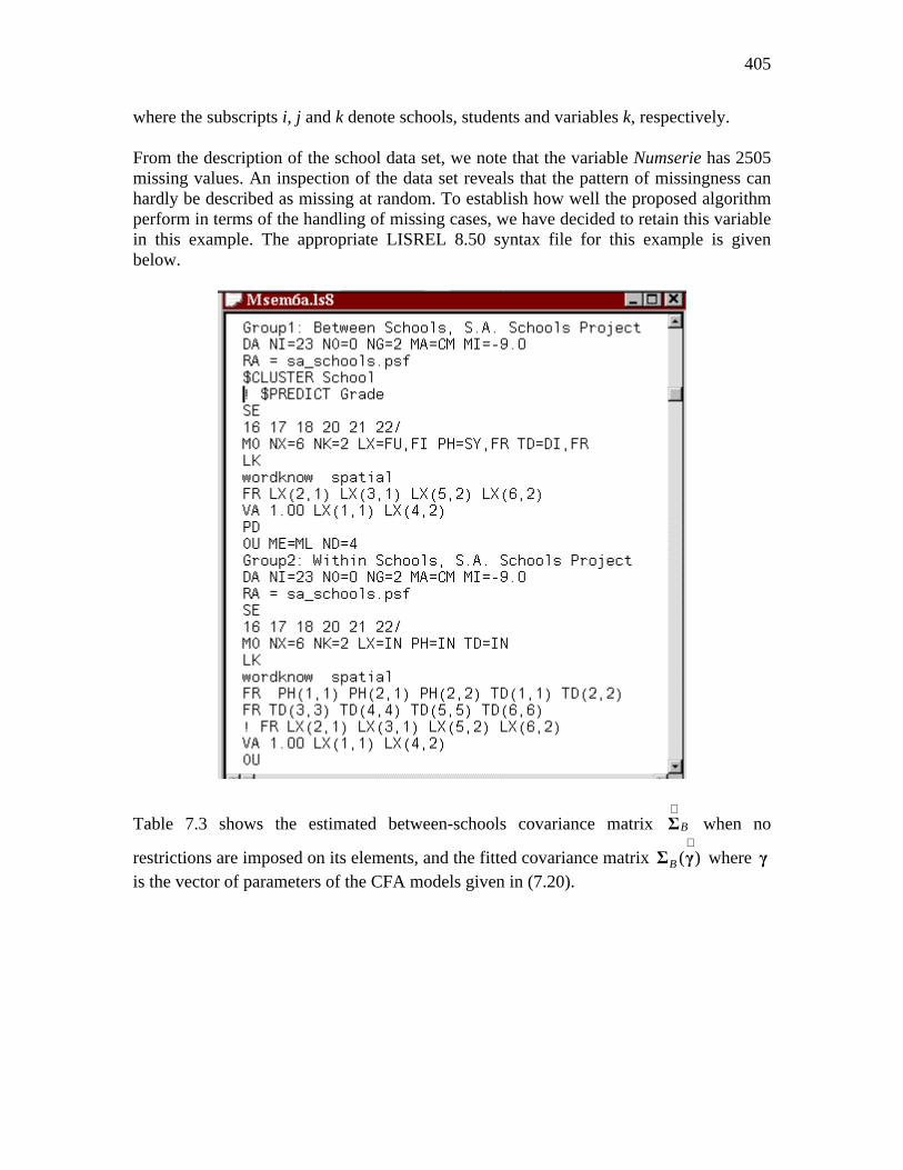
where the subscripts i, j and k denote schools, students and variables k, respectively. From the description of the school data set, we note that the variable Numserie has 2505 missing values. An inspection of the data set reveals that the pattern of missingness can hardly be described as missing at random. To establish how well the proposed algorithm perform in terms of the handling of missing cases, we have decided to retain this variable in this example. The appropriate LISREL 8.50 syntax file for this example is given below.

Table 7.3 shows the estimated between-schools covariance matrix B

∧Σ when no

restrictions are imposed on its elements, and the fitted covariance matrix ( )B

∧Σ γ where γ

is the vector of parameters of the CFA models given in (7.20).

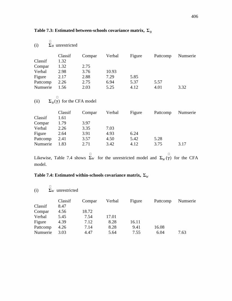
406

Table 7.3: Estimated between-schools covariance matrix, BΣ

(i) B

∧Σ unrestricted

Classif Compar Verbal Figure Pattcomp Numserie Classif 1.32 Compar 1.32 2.75 Verbal 2.98 3.76 10.93 Figure 2.17 2.88 7.29 5.85 Pattcomp 2.26 2.75 6.94 5.37 5.57 Numserie 1.56 2.03 5.25 4.12 4.01 3.32

(ii) ( )B

∧Σ γ for the CFA model

Classif Compar Verbal Figure Pattcomp Numserie Classif 1.61 Compar 1.79 3.97 Verbal 2.26 3.35 7.03 Figure 2.64 3.91 4.93 6.24 Pattcomp 2.41 3.57 4.50 5.42 5.28 Numserie 1.83 2.71 3.42 4.12 3.75 3.17

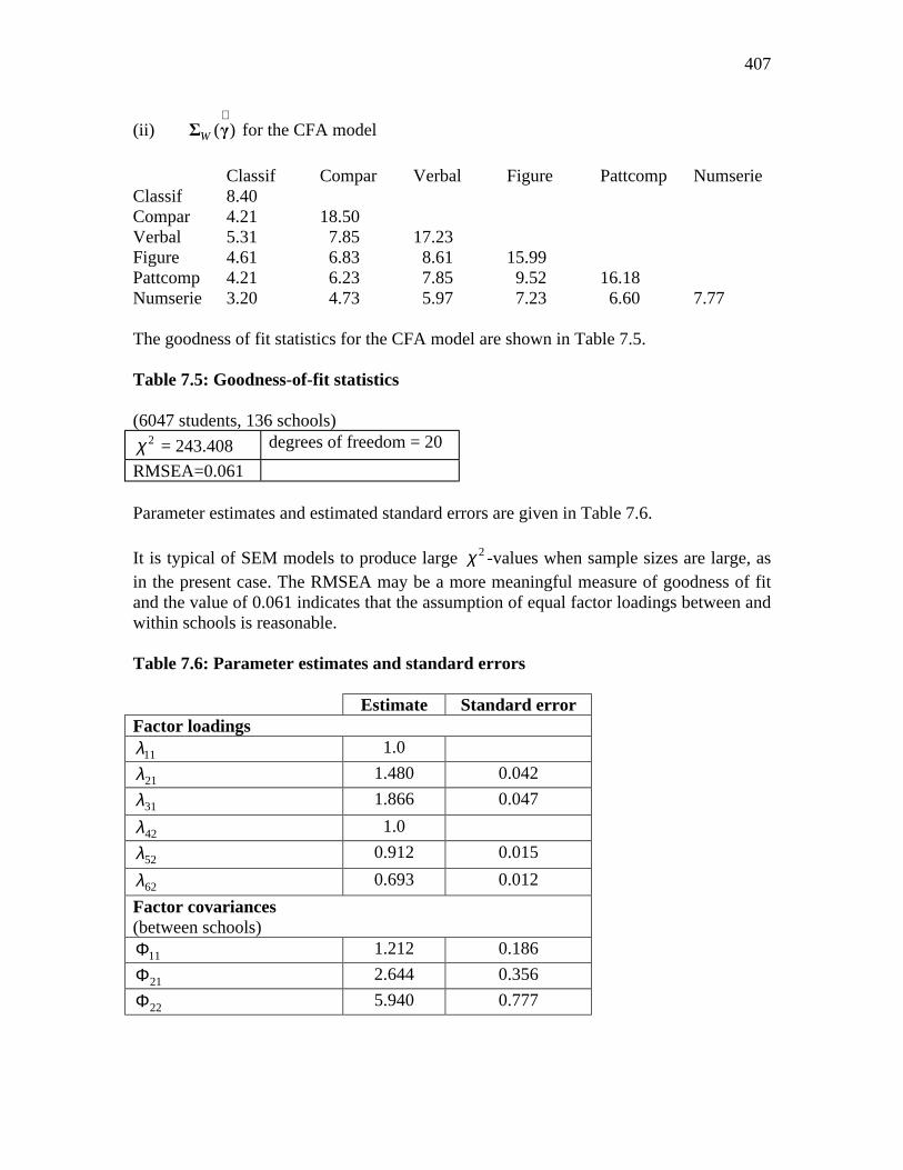
Likewise, Table 7.4 shows W

∧Σ for the unrestricted model and ( )W

∧Σ γ for the CFA

model. Table 7.4: Estimated within-schools covariance matrix, WΣ

(i) W

∧Σ unrestricted

Classif Compar Verbal Figure Pattcomp Numserie Classif 8.47 Compar 4.56 18.72 Verbal 5.45 7.54 17.01 Figure 4.39 7.12 8.28 16.11 Pattcomp 4.26 7.14 8.28 9.41 16.08 Numserie 3.03 4.47 5.64 7.55 6.04 7.63

407

(ii) ( )W

∧Σ γ for the CFA model

Classif Compar Verbal Figure Pattcomp Numserie Classif 8.40 Compar 4.21 18.50 Verbal 5.31 7.85 17.23 Figure 4.61 6.83 8.61 15.99 Pattcomp 4.21 6.23 7.85 9.52 16.18 Numserie 3.20 4.73 5.97 7.23 6.60 7.77 The goodness of fit statistics for the CFA model are shown in Table 7.5. Table 7.5: Goodness-of-fit statistics (6047 students, 136 schools)

2χ = 243.408 degrees of freedom = 20

RMSEA=0.061 Parameter estimates and estimated standard errors are given in Table 7.6. It is typical of SEM models to produce large 2χ -values when sample sizes are large, as in the present case. The RMSEA may be a more meaningful measure of goodness of fit and the value of 0.061 indicates that the assumption of equal factor loadings between and within schools is reasonable. Table 7.6: Parameter estimates and standard errors Estimate Standard error Factor loadings

11λ 1.0

21λ 1.480 0.042

31λ 1.866 0.047

42λ 1.0

52λ 0.912 0.015

62λ 0.693 0.012

Factor covariances (between schools)

11Φ 1.212 0.186

21Φ 2.644 0.356

22Φ 5.940 0.777

408

Table 7.6: Parameter estimates and standard errors (continued) Estimate Standard error Error variances (between schools) Classif 0.399 0.078 Compar 1.321 0.221 Verbal 2.811 0.400 Figure 0.304 0.091 Pattcomp 0.333 0.089 Numserie 0.314 0.068 Factor covariances (within schools)

11Φ 2.844 0.127

21Φ 4.615 0.146

22Φ 10.437 0.298

Error variances (within schools) Classif 5.554 0.119 Compar 12.276 0.263 Verbal 7.328 0.225 Figure 5.553 0.168 Pattcomp 7.496 0.183 Numserie 2.760 0.098

7.5 Multilevel Non-Linear Models

7.5.1 Introduction to Multilevel Modeling

The analysis of data with a hierarchical structure has been described in the literature under various names. It is known as hierarchical modeling, random coefficient modeling, latent curve modeling, growth curve modeling or multilevel modeling. The basic underlying structure of measurements nested within units at a higher level of the hierarchy is, however, common to all. In a repeated measurements growth model, for example, the measurements or outcomes are nested within the experimental units (second level units) of the hierarchy. Ignoring the hierarchical structure of data can have serious implications, as the use of alternatives such as aggregation and disaggregation of information to another level can induce high collinearity among predictors and large or biased standard errors for the estimates. Standard fixed parameter regression models do not allow for the exploration of variation between groups, which may be of interest in its own right. For a discussion of

409

the effects of these alternatives, see Bryk and Raudenbush (1992), Longford (1987) and Rasbash (1993). Multilevel or hierarchical modeling provides the opportunity to study variation at different levels of the hierarchy. Such a model can also include separate regression coefficients at different levels of the hierarchy that have no meaning without recognition of the hierarchical structure of the population. The dependence of repeated measurements belonging to one experimental unit in a typical growth curve analysis, for example, is taken into account with this approach. In addition, the data to be analyzed need not be balanced in nature. This has the advantage that estimates can also be units for which a very limited amount of information is available.

7.5.2 Multilevel Non-Linear Regression Models

It was pointed out by Pinheiro and Bates (2000) that one would want to use nonlinear latent coefficient models for reasons of interpretability, parsimony, and more importantly, validity beyond the observed range of the data. By increasing the order of a polynomial model, one can get increasingly accurate approximations to the true, usually nonlinear, regression function, within the range of the observed data. High order polynomial models often result in multicollinearity problems and provide no theoretical considerations about the underlying mechanism producing the data.

There are many possible nonlinear regression models to select from. Examples are given by Gallant (1987) and Pinheiro and Bates (2000). The Richards function (Richards, 1959) is a generalization of a family of non-linear functions and is used to describe growth curves (Koops, 1988). Three special cases of the Richards function are the logistic, Gompertz and Monomolecular functions, respectively. Presently, one can select curves of the form

1 2( ) ( )y f x f x e= + +

where the first component, 1( )f x may have the form:

• logistic: 1

2 3(1 exp( )

b

s b b x+ −

• Gompertz: 1 2 3exp( exp( ))b b b x− −

• Monomolecular: 1 2 3(1 exp( ))b s b b x+ −

• power: 21

bb x

• exponential: 1 2exp( )b b x−

410

The second component, 2 ( )f x , may have the form:

• logistic: 1

2 3(1 exp( )

c

s c c x+ −

• Gompertz: 1 2 3exp( exp( ))c c c x− −

• Monomolecular: 1 2 3(1 exp( ))c s c c x+ −

• power: 21

cc x

• exponential: 1 2exp( )c c x− In the curves above s denotes the sign of the term 2 3exp( )b b x− and is equal to 1 or -1.

Since the parameters in the first three functions above have definite physical meanings, a curve from this family is preferred to a polynomial curve, which may often be fitted to a set of responses with the same degree of accuracy. The parameter 1b represents the time

asymptotic value of the characteristic that has been measured, the parameter 2b represents the potential increase (or decrease) in the value of the function during the course of time 1t to pt , and the parameter 3b characterizes the rate of growth.

The coefficients 1 2 3, , ,b b c… are assumed to be random, and, as in linear hierarchical

models, can be written as level-2 outcome variables where

1 1 1

2 2 2

3 3 3

1 4 4

2 5 5

3 6 6.

b u

b u

b u

c u

c u

c u

ββββββ

= += += += += += +

It is assumed that the level-2 residuals 1 2 6, , ,u u u… have a normal distribution with zero

means and covariance matrix Φ . In LISREL, it may further be assumed that the values of any of the random coefficients are affected by some level-2 covariate so that, in general,

1 1 1 1 1

2 2 2 2 2

3 3 3 3 3

1 4 4 4 4

2 5 5 5 5

3 6 6 6 6.

b z u

b z u

b z u

c z u

c z u

c z u

β γβ γβ γβ γβ γβ γ

= + += + += + += + += + += + +

411

where iz denotes the value of a covariate and iγ the corresponding coefficient.

It is usually sufficient to select a single component 1( ( ))f x to describe a large number of monotone increasing (or decreasing) growth patterns. To describe more complex patterns, use can be made of two-component regression models. LISREL allows the user to select any of the 5 curve types as component 1 and to combine it with any one of the 5 curve types for the second component. Valid choices are, for example,

• Monomolecular + Gompertz • logistic • exponential + logistic • logistic + logistic

The unknown model parameters are the vector of fixed coefficients ( )β , the vector of covariate coefficients ( )γ , the covariance matrix ( )Φ of the level-2 residuals and the

variance 2( )σ of the level-1 measurement errors. See Chapter 5 for an example of fitting of a multilevel nonlinear model. Additional examples are given in the nonlinex folder.

7.5.3 Estimation Procedure for Multilevel Non-Linear Regression Models

In linear multilevel models, y has a normal distribution, since y is a linear combination of the random coefficients. For example, the intercept-and-slopes-as-outcomes model is

1 2y b b x e= + + where 1 1 2 2,b u b u= = and 1 2( , )u u is assumed to be normally distributed. A multilevel nonlinear model is a regression model which cannot be expressed as a linear combination of its coefficients and therefore y is no longer normally distributed. The probability density function of y can be evaluated as the multiple integral

1 3

1 3 1 3( ) ( , , , )b c

f y f y b c db dc= ∫ ∫… … …

that, in general, cannot be solved in closed form.

412

To evaluate the likelihood function

1

( )n

ii

L f y=

=∏ ,

one has to use a numerical integration technique. We assume that e has a 2(0, )N σ

distribution and that 1 2 3 1 2 3( , , , , , )b b b c c c has a 2( , )N 0 Φ distribution.

In the multilevels procedure, use is made of a Gauss quadrature procedure to evaluate the integrals numerically. The ML method requires good starting values for the unknown parameters. The estimation procedure is described by Cudeck and du Toit (in press).

Starting values Once a model is selected to describe the nonlinear pattern in the data, for example as revealed by a plot of y on x, a curve is fitted to each individual using ordinary non-linear least squares. In step 1 of the fitting procedure, these OLS parameter estimates are written to a file and estimates of β and Φ are obtained by using the sample means and covariances of the set of fitted parameters. Since observed values from some individual cases may not be adequately described by the selected model, these cases can have excessively large residuals, and it may not be advisable to include them in the calculation of the β and Φ estimates. In step 2 of the model fitting procedure, use is made of the MAP (Maximum Aposterior) estimator of the unknown parameters. Suppose that a single component 1( , )f b x is fitted to the data. Since

( | ) ( ) ( | ) / ( ),f b y f b f y b f y=

where ( | )f b y is the conditional probability density function of the random coefficients b given the observations, it follows that

ln ( | ) ln ( ) ln ( | ) ,f b y f b f y b k= + +

where ln ( )k f y= − .

413

The MAP procedure can briefly be described as follows:

Step a:

Given starting values of β , Φ and 2σ , obtain estimates of the random coefficients ib∧

from

ln ( | ) 0, 1,2, , .i ii

f b y i nb

∂ = =∂

…

Step b:

Use the estimates 1 2, , , nb b b∧ ∧ ∧

… and 1( ), , ( )nCov b Cov b∧ ∧… to obtain new estimates of β ,

Φ and 2σ (see Herbst, A. (1993) for a detailed discussion). Repeat steps a and b until convergence is attained. For many practical purposes, results obtained from the MAP procedure may be sufficient. However, if covariates are included in the model, parameter estimates are only available via the ML option, which uses the MAP estimates of β , Φ and 2σ as starting values.

7.6 FIRM: Formal Inference-based Recursive Modeling

7.6.1 Overview

Recursive modeling is an attractive data-analytic tool for studying the relationship between a dependent variable and a collection of predictor variables. In this, it complements methods such as multiple regression, analysis of variance, neural nets, generalized additive models, discriminant analysis and log linear modeling. It is particularly helpful when simple models like regression do not work, as happens when the relationship connecting the variables is not straightforward—for example if there are synergies between the predictors. It is attractive when there is missing information in the data. It can also be valuable when used in conjunction with a more traditional statistical data analysis, as it may provide evidence that the model assumptions underlying the traditional analysis are valid, something that is otherwise not easy to do.

414

The output of a recursive model analysis is a “dendrogram”, or “tree diagram”. This shows how the predictors can be used to partition the data into successively smaller and more homogeneous subgroups. This dendrogram can be used as an immediate pictorial way of making predictions for future cases, or “interpreted” in terms of the effects on the dependent variable of changes in the predictor. The maximum problem size the codes distributed in this package can handle is 1000 predictors; the number of cases is limited only by the available disk space. Recursive partitioning (RP) is not attractive for all data sets. Going down a tree leads to rapidly diminishing sample sizes and the analysis comes to an end quite quickly if the initial sample size was small. As a rough guide, the sample size needs to be in three digits before recursive partitioning is likely to be worth trying. Like all feature selection methods, it is also highly non-robust in the sense that small changes in the data can lead to large changes in the output. The results of a RP analysis therefore always need to be thought of as a model for the data, rather than as the model for the data. Within these limitations though, the recursive partitioning analysis gives an easy, quick way of getting a picture of the relationship that may be quite different than that given by traditional methods, and that is very informative when it is different. FIRM is made available through LISREL by the kind permission of the author, Professor Douglas M. Hawkins, Department of Applied Statistics, University of Minnesota. Copyright of the FIRM documentation: Douglas M. Hawkins, Department of Applied Statistics, University of Minnesota, 352 COB, 1994 Buford Ave, St. Paul, MN 55108 1990, 1992, 1995, 1997, 1999

7.6.2 Recursive Partitioning Concepts

The most common methods of investigating the relationship between a dependent variable Y and a set of predictors 1 2, , , pX X X… are the linear model (multiple

regression, analysis of variance and analysis of covariance) for a continuous dependent variable, and the log linear model for a categorical dependent. Both methods involve strong model assumptions. For example, multiple regression assumes that the relationship between Y and the iX is linear, that there are no interaction terms other than those

explicitly included in the model; and that the residuals satisfy strong statistical assumptions of a normal distribution and constant variance. The log linear model for categorical data assumes that any interaction terms not explicitly included are not needed; while it provides an overall 2χ test-of-fit of the model, when this test fails it does not help to identify what interaction terms are needed. Discriminant analysis is widely used to find rules to classify observations into the different populations from which they came.

415

It is another example of a methodology with strong model assumptions that are not easy to check. A different and in some ways diametrically opposite approach to all these problems is modeling by recursive partitioning. In this approach, the calibration data set is successively split into ever-smaller subsets based on the values of the predictor variables. Each split is designed to separate the cases in the node being split into a set of successor groups, which are in some sense maximally internally homogeneous.

An example of a data set in which FIRM is a potential method of analysis is the “head injuries” data set of Titterington et al (1981) (data kindly supplied by Professor Titterington). As we will be using this data set to illustrate the operation of the FIRM codes, and since the data set is included in the FIRM distribution for testing purposes, it may be appropriate to say something about it. The data set was gathered in an attempt to predict the final outcome of 500 hospital patients who had suffered head injuries. The outcome for each patient was that he or she was: • Dead or vegetative (52% of the cases); • had severe disabilities (10% of the cases); • or had a moderate or good recovery (38% of the cases). This outcome is to be predicted on the basis of 6 predictors assessed on the patients’ admission to the hospital: • Age : The age of the patient. This was grouped into decades in the original data, and

is grouped the same way here. It has eight classes. • EMV : This is a composite score of three measures—of eye-opening in response to

stimulation; motor response of best limb; and verbal response. This has seven classes, but is not measured in all cases, so that there are eight possible codes for this score, these being the seven measurements and an eighth “missing” category.

• MRP : This is a composite score of motor responses in all four limbs. This also has seven measurement classes with an eighth class for missing information.

• Change : The change in neurological function over the first 24 hours. This was graded 1, 2 or 3, with a fourth class for missing information.

• Eye indicator : A summary of diagnostics on the eyes. This too had three measurement classes, with a fourth for missing information.

• Pupils : Eye pupil reaction to light, namely present, absent, or missing.

7.6.3 CATFIRM

Figure 7.3 is a dendrogram showing the end result of analyzing the data set using the CATFIRM syntax, which is used for a categorical dependent variable like this one. Syntax can be found in the file headicat.pr2.

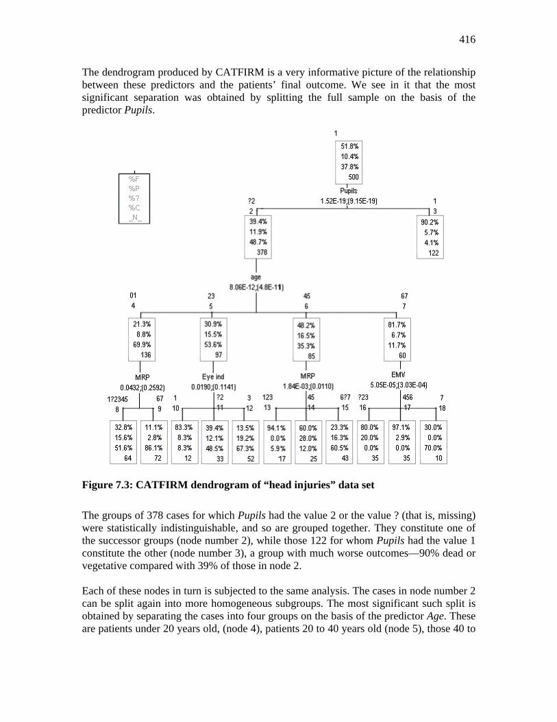
416

The dendrogram produced by CATFIRM is a very informative picture of the relationship between these predictors and the patients’ final outcome. We see in it that the most significant separation was obtained by splitting the full sample on the basis of the predictor Pupils.

Figure 7.3: CATFIRM dendrogram of “head injuries” data set

The groups of 378 cases for which Pupils had the value 2 or the value ? (that is, missing) were statistically indistinguishable, and so are grouped together. They constitute one of the successor groups (node number 2), while those 122 for whom Pupils had the value 1 constitute the other (node number 3), a group with much worse outcomes—90% dead or vegetative compared with 39% of those in node 2. Each of these nodes in turn is subjected to the same analysis. The cases in node number 2 can be split again into more homogeneous subgroups. The most significant such split is obtained by separating the cases into four groups on the basis of the predictor Age. These are patients under 20 years old, (node 4), patients 20 to 40 years old (node 5), those 40 to

417

60 years old (node 6) and those over 60 (node 7). The prognosis of these patients deteriorates with increasing age; 70% of those under 20 ended with moderate or good recoveries, while only 12% of those over 60 did. Node 3 is terminal. Its cases cannot (at the significance levels selected) be split further. Node 4 can be split using MRP. Cases with MRP = 6 or 7 constitute a group with a favorable prognosis (86% with moderate to good recovery); and the other MRP levels constitute a less-favorable group but still better than average. These groups, and their descendants, are analyzed in turn in the same way. Ultimately no further splits can be made and the analysis stops. Altogether 18 nodes are formed, of which 12 are terminal and the remaining 6 intermediate. Each split in the dendrogram shows the variable used to make the split and the values of the splitting variable that define each descendant node. It also lists the statistical significance (p-value) of the split. Two p-values are given: that on the left is FIRM’s conservative p-value for the split. The p-value on the right is a Bonferroni-corrected value, reflecting the fact that the split actually made had the smallest p-value of all the predictors available to split that node. So for example, on the first split, the actual split made has a p-value of 191.52 10−× . But when we recognize that this was selected because it was the most significant of the 6 possible splits, we may want to scale up its p-value by the factor 6 to allow for the fact that it was the smallest of 6 p-values available (one for each predictor). This gives its conservative Bonferroni-adjusted p-value as 199.15 10−× . The dendrogram and the analysis giving rise to it can be used in two obvious ways: for making predictions, and to gain understanding of the importance of and interrelationships between the different predictors. Taking the prediction use first, the dendrogram provides a quick and convenient way of predicting the outcome for a patient. Following patients down the tree to see into which terminal node they fall yields 12 typical patient profiles ranging from 96% dead/vegetative to 100% with moderate to good recoveries. The dendrogram is often used in exactly this way to make predictions for individual cases. Unlike, say, predictions made using multiple regression or discriminant analysis, the prediction requires no arithmetic—merely the ability to take a future case “down the tree”. This allows for quick predictions with limited potential for arithmetic errors. A hospital could, for example, use Figure 7.3 to give an immediate estimate of a head-injured patient’s prognosis. The second use of the FIRM analysis is to gain some understanding of the predictive power of the different variables used and how they interrelate. There are many aspects to this analysis. An obvious one is to look at the dendrogram, seeing which predictors are used at the different levels. A rather deeper analysis is to look also at the predictors that were not used to make the split in each node, and see whether they could have discriminated between different subsets of cases. This analysis is done using the “summary” file part of the output, which can be requested by adding the keyword sum on the first line of the syntax file. In this head injuries data set, the summary file shows that all 6 predictors are very discriminating in the full data set, but are much less so as soon as

418

the initial split has been performed. This means that there is a lot of overlap in their predictive information: that different predictors are tapping into the same or related basic physiological indicators of the patient’s state. Another feature often seen is an interaction in which one predictor is predictive in one node, and a different one is predictive in another. This may be seen in this data set, where Age is used to split Node 4, but Eye ind is used to split Node 5. Using different predictors at different nodes at the same level of the dendrogram is one example of the interactions that motivated the ancestor of current recursive partitioning codes—the Automatic Interaction Detector (AID). Examples of diagnosing interactions from the dendrogram are given in Hawkins and Kass (1982).

7.6.4 CONFIRM

Figure 7.3 illustrates the use of CATFIRM, which is appropriate for a categorical dependent variable. The other analysis covered by the FIRM package is CONFIRM, which is used to study a dependent variable on the interval scale of measurement. Figure 7.4 shows an analysis of the same data using CONFIRM. The dependent variable was on a three-point ordinal scale, and for the CONFIRM analysis we treated it as being on the interval scale of measurement with values 1, 2 and 3 scoring 1 for the outcome “dead or vegetative”; 2 for the outcome “severe disability” and 3 for the outcome “moderate to good recovery”. As the outcome is on the ordinal scale, this equal-spaced scale is not necessarily statistically appropriate in this data set and is used as a matter of convenience rather than with the implication that it may be the best way to proceed. The full data set of 500 cases has a mean outcome score of 1.8600. The first split is made on the basis of the predictor Pupils. Cases for which Pupils is 1 or ? constitute the first descendant group (Node 2), while those for which it is 2 give Node 3. Note that this is the same predictor that CATFIRM elected to use, but the patients with missing values of Pupils are grouped with Pupils = 1 by the CONFIRM analysis, and with Pupils = 2 by CATFIRM. Going to the descendant groups, Node 2 is then split on MRP (unlike in CATFIRM, where the corresponding node was terminal), while Node 3 is again split four ways on Age. The overall tree is bigger than that produced by CATFIRM—13 terminal and 8 interior nodes—and produces groups with prognostic scores ranging from a grim 1.0734 up to 2.8095 on the 1 to 3 scale. As with CATFIRM, the means in these terminal nodes could be used for prediction of future cases, giving estimates of the score that patients in the terminal nodes would have. The statistical model used in CONFIRM can be described as a piecewise constant regression model. For example, among the patients in Node 3, the outcome is predicted to be 2.48 for patients aged under 20, 2.25 for those aged 20 to 40, 1.88 for those aged 40 to 60, and 1.32 for those aged over 60. This approach contrasts sharply with, say, a linear regression in which the outcome would be predicted to rise by some constant amount

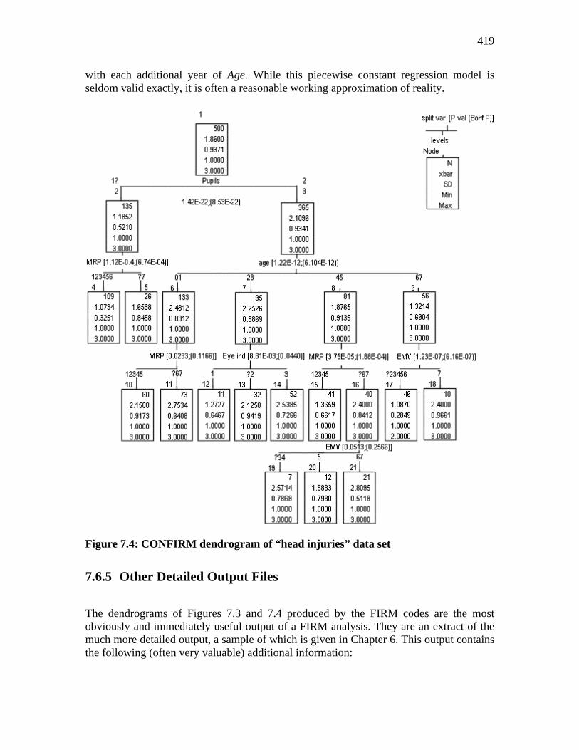
419

with each additional year of Age. While this piecewise constant regression model is seldom valid exactly, it is often a reasonable working approximation of reality.

Figure 7.4: CONFIRM dendrogram of “head injuries” data set

7.6.5 Other Detailed Output Files

The dendrograms of Figures 7.3 and 7.4 produced by the FIRM codes are the most obviously and immediately useful output of a FIRM analysis. They are an extract of the much more detailed output, a sample of which is given in Chapter 6. This output contains the following (often very valuable) additional information:

420

• An analysis of each predictor in each node, showing which categories of the predictor FIRM finds it best to group together, and what the conservative statistical significance level of the split by each predictor is;

• The number of cases owing into each of the descendant groups; • Summary statistics of the cases in the descendant nodes. In the case of CATFIRM,

the summary statistics are a frequency breakdown of the cases between the different classes of the dependent variable. With CONFIRM, the summary statistics given are the arithmetic mean and standard deviation of the cases in the node. This summary information is echoed in the dendrogram.

7.6.6 FIRM Building Blocks

There are three elements to analysis by a recursive partitioning method such as FIRM: • deciding which predictor to use to define the split; • deciding which categories of the predictor should be grouped together so that the data

set is not split more ways than are really necessary (for example, is a binary, three-way, four-way etc. split on this variable required); and

• deciding when to stop growing the tree. Different implementations of recursive partitioning handle these issues in different ways. The theoretical basis for the procedures implemented in FIRM and used to produce these dendrograms is set out in detail in Hawkins and Kass (1982) and Kass (1980). Readers interested in the details of the methodology should refer to these two sources and to the papers they reference. The Ph.D. thesis by Kass (1972) included a PL/1 program for CHAID (“chi-squared automatic interaction detector”)—CATFIRM is based on a translation of this code into FORTRAN. The methodology (but no code) is set out in a perhaps more widely accessible medium in the paper by Kass (1975). The 1981 technical report by Heymann discusses a code XAID (“extended automatic interaction detector”) which extended the framework underlying CHAID to an interval-scale dependent variable. CONFIRM is a development of this program. The FIRM methodology has been applied to a wide variety of problems—for example, Hooton et al (1981) was an early application in medicine, and Hawkins, Young and Rusinko (1997) illustrates an application to drug discovery. After this brief illustration of two FIRM runs, we will now go into some of the underlying ideas of the methodology. Readers who have not come across recursive partitioning before would be well advised to experiment with the CONFIRM and CATFIRM before going too far into this detail. See Chapter 6 for FIRM examples and also the firmex folder.

421

7.6.7 Predictor and Dependent Variable Types

Writings on measurement types often distinguish four scales of measurement: • Nominal, in which the measurement divides the individuals studied into different

classes. Eye color is an example of a nominal measure on a person. • Ordinal, in which the different categories have some natural ordering. Social class is

an example of an ordinal measure. So is a rating by the adjectives “Excellent”, “Very good”, “Good”, “Fair”, “Poor”.

• Interval, in which a given difference between two values has the same meaning wherever these values are in the scale. Temperature is an example of a measurement on the interval scale—the temperature difference between 10 and 15 degrees is the same as that between 25 and 30 degrees.

• Ratio, which goes beyond the interval scale in having a natural zero point. Each of these measurement scales adds something to the one above it, so an interval measure is also ordinal, but an ordinal measure is generally not interval. FIRM can handle two types of dependent variable: those on the nominal scale (analyzed by CATFIRM), and those on the interval scale (analyzed by CONFIRM). There is no explicit provision for a dependent variable on the ordinal scale such as, for example, a qualitative rating “Excellent”, “Good”, “Fair” or “Poor”. Dependents like this have to be handled either by ignoring the ordering information and treating them using CATFIRM, or by trying to find an appropriate score for the different categories. These scores could range from the naive (for example the 1-2-3 scoring we used to analyze the head injuries data with CONFIRM) to conceptually sounder scorings obtained by scaling methods. Both FIRM approaches use the same predictor types and share a common underlying philosophy. While FIRM recognizes five predictor types, two going back to its Automatic Interaction Detection roots are fundamental: • Nominal predictors (which are called “free” predictors in the AID terminology), • Ordinal predictors (which AID labels “monotonic” predictors). In practical use, some ordinal predictors are just categorical predictors with ordering among their scales, while others are interval-scaled. Suppose for example that you are studying automobile repair costs, and think the following predictors may be relevant: • make: The make of the car. Let’s suppose that in the study it is sensible to break this

down into 5 groupings: GM, Ford, Chrysler, Japanese and European. • cyl: The number of cylinders in the engine: 4, 6, 8 or 12. • price: The manufacturer’s suggested retail purchase price when new. • year: The year of manufacture.

422

make is clearly nominal, and so would be used as a free predictor. In a linear model analysis, you would probably use analysis of variance, with make a factor. Looking at these predictors, cyl seems to be on the interval scale, and so might be used as an ordered (monotonic) predictor. If we were to use cyl in a linear regression study, we would be making a strong assumption that the repair costs difference between a 4- and an 8-cylinder car is the same as that between an 8- and a 12-cylinder car. FIRM’s monotonic predictor type involves no such global assumption. price is a ratio-scale predictor that would be specified as monotonic—it seems generally accepted that cars that are more expensive to buy are also more expensive to maintain. In fact, though, even if this were false, so long as the relationship between price and repair costs was reasonably smooth (and not necessarily even monotonic) FIRM’s piecewise constant model fitting would be able to handle it.

Finally, year is an example of a predictor that looks to be on an interval scale (since a one-year gap is a one-year gap whether it is the gap between 1968 and 1969 or that between 1998 and 1999), but appearances may be deceptive. While some years’ cars do certainly seem to be more expensive to maintain than other years’ cars, it is not obvious that this relationship is a smooth one. A “lemon” year can be preceded and followed by years in which a manufacturer makes good, reliable cars. For this reason it would be preferable to make year a free predictor rather than monotonic. This will allow the cost to have any type of response to year, including one in which certain isolated years are bad while their neighbors are good. If the repair cost should turn out to vary smoothly with year then little would have been lost and that little could be recovered by repeating the run, respecifying year as monotonic.

7.6.8 Internal Grouping to get Starting Groups

Internally, the FIRM code requires all predictors to be reduced to a modest number (no more than 16 or 20) of distinct categories, and from this starting set it will then merge categories until it gets to the final grouping. Thus in the car repair cost example, make, cyl and possibly year are ready to run. The predictor price is continuous—it likely takes on many different values. For FIRM analysis it would therefore have to be categorized into a set of price ranges. There are two ways of doing this: you may decide ahead of time what sensible price ranges are and use some other software to replace the dollar value of the price by a category number. This option is illustrated by the predictor Age in the “head injuries” data. A person’s age is continuous, but in the original data set it had already been coded into decades before we got the data, and this coded value was used in the FIRM.

You can also have FIRM do the grouping for you. It will attempt to find nine initial working cutpoints, breaking the data range into 10 initial classes. The downside of this is that you may not like its selection of cutpoints: if we had had the subjects’ actual ages in

423

the head injuries data set, FIRM might have chosen strange-looking cutpoints like 14, 21, 27, 33, 43, 51, 59, 62, 68 and 81. These are not as neat or explainable as the ages by decades used by Titterington, et al.

Either way of breaking a continuous variable down into classes introduces some approximation. Breaking age into decades implies that only multiples of 10 years can be used as split points in the FIRM analysis. This leaves the possibility that, when age was used to split node 3 in CATFIRM with cut points at ages 20, 40 and 60, better fits might have been obtained had ages between the decade anniversaries been allowed as possible cut points: perhaps it would have been better to split at say age 18 rather than 20, 42 rather than 40 and 61 rather than 60. Maybe a completely different set of cut points could have been chosen. All this, whether likely or not, is certainly possible, and should be borne in mind when using continuous predictors in FIRM analysis.

Internally, all predictors in a FIRM analysis will have values that are consecutive integers, either because they started out that way or because you allowed FIRM to translate them to consecutive integers. This is illustrated by the “head injuries” data set. All the predictors had integer values like 1,2,3. Coding the missing information as 0 then gave a data set with predictors that were integer valued.

7.6.9 Grouping the Categories

The basic operation in modeling the effect of some predictor is the reduction of its values to different groups of categories. FIRM does this by testing whether the data corresponding to different categories of the dependent variable differ significantly, and if not, it puts these categories together. It does this differently for different types of predictors: • free predictors are on the nominal scale. When categories are tested for possibly being

together, any classes of a free predictor may be grouped. Thus in the car repairs, we could legitimately group any of the categories GM, Ford, Chrysler, Japanese and European together.

• monotonic predictors are on the ordinal scale. One example might be a rating with options “Poor”, “Fair”, “Good”, “Very good” and “Excellent”. Internally, these values need to be coded as consecutive integers. Thus in the “head injuries” data the different age groups were coded as 1, 2, 3, 4, 5, 6, 7 and 8. When the classes of a predictor are considered for grouping, only groupings of contiguous classes are allowed. For example, it would be permissible to pool by age into the groupings {1,2}, {3}, {4,5,6,7,8}, but not into {1,2}, {5,6}, {3,4,7,8}, which groups ages 3 and 4 with 7 and 8 while excluding the intermediate ages 4 and 5.

The term “monotonic” may be misleading as it suggests that the dependent variable has to either increase or decrease monotonically as the predictor increases. Though this is

424

usual when you specify a predictor as monotonic, it is not necessarily so. FIRM fits “step functions”, so it could be sensible to specify a predictor as monotonic if the dependent variable first increased with the predictor and then decreased, so long as the response was fairly smooth.

Consider, for example, using a person’s age to predict physical strength. If all subjects were aged under, say, 18, then strength would be monotonically increasing with age. If all subjects were aged over 25, then strength would be monotonically decreasing with age. If the subjects span both age ranges, then the relationship would be initially increasing, then decreasing. Using age as a monotonic predictor will still work correctly in that only adjacent age ranges will be grouped together. The fitted means, though, would show that there were groups of matching average strength at opposite ends of the age spectrum.

If you have a predictor that is on the ordinal scale, but suspect that the response may not be smooth, then it would be better, at least initially, to specify it as free and then see if the grouping that came back looked reasonably monotonic. This would likely be done in the car repair costs example with the predictor year.

7.6.10 Additional Predictor Types

These are the two basic predictor types inherited from FIRM’s roots in AID. In addition to these, FIRM has another three predictor types: 1. The floating predictor is a variant of the monotonic predictor. A floating predictor is

one whose scale is monotonic except for a single “floating” class whose position in the monotonic scale is unknown. This type is commonly used to handle a predictor which is monotonic but which has missing values on some cases. The rules of grouping are that the monotonic portion of the scale can be grouped only monotonically, but that the floating class may be grouped with any other class or classes on the scale. Like the free and monotonic predictors, this predictor type must also be coded in the data set as consecutive integers, and in these implementations of FIRM, the missing class is required to be the first one. So for example you might code a math grade of A, B, C, D, F or missing as 0 for missing, with A, B, C, D and F coded as 1, 2, 3, 4 and 5, for a total of 6 categories.

2. A real predictor is continuous: for example, the purchase price of the automobile; a patient’s serum cholesterol level; a student’s score in a pretest. FIRM handles real predictors by finding 9 cutpoints that will divide the range of values of the predictor into 10 classes of approximately equal frequency. Putting the predictor into one of these classes then gives a monotonic predictor. The real predictor may contain missing values. FIRM interprets any value in the data set that is not a valid number to be missing. For example, if a real predictor is being read from a data set and the value recorded is ? or . or M, then the predictor is taken to be missing on that case. Any real

425

predictor that has missing values will be handled as a floating predictor—the missing category will be isolated as one category and the non-missing values will be broken down into the 10 approximately equal-frequency classes.

3. A character predictor is a free predictor that has not been coded into successive digits. For example, if gender is a predictor, it may be represented by M, F and ? in the original data base. To use it in FIRM, you could use some other software to recode the data base into, say, 1 for M, 2 for F, and 0 for ?, and treat it as a free predictor. Or you could just leave the values as is, and specify to FIRM that the predictor is of type character. FIRM will then find the distinct gender codes automatically. The character predictor type can also sometimes be useful when the predictor is integer- valued, but not as successive integers. For example, the number of cylinders of our hypothetical car, 4, 6, 8 or 12, would best be recoded as 1, 2, 3 and 4, but we could declare it character and let FIRM find out for itself what different values are present in the data. Releases of FIRM prior to 2.0 supported only free, monotonic and floating predictors. FIRM 2.0 and up implement the real and character types by internally recoding real predictors as either monotonic or floating predictors, and character as free predictors. Having a variable as type character does not remove the restriction on the maximum number of distinct values it can have—this remains at 16 for CATFIRM and (in the current release) 20 for CONFIRM. As of FIRM 2.0, the dependent variable in CATFIRM may also be of type character. With this option, CATFIRM can find out for itself what are the different values taken on by the dependent variable.

7.6.11 Missing Information and Floating Predictors

The monotonic and free predictor types date right back to the early 1960s implementation of AID; the real and character predictor types are essentially just an extra code layer on top of the basic types to make them more accessible. As the floating predictor type is newer, and also is not supported by all recursive modeling procedures, some comments on its potential uses may be helpful. The floating predictor type is mainly used for handling missing information in an otherwise ordinal predictor. Most procedures for handling missing information have at some level an underlying “missing at random” assumption. This assumption is not always realistic: there are occasions in which the fact that a predictor is missing in a case may itself convey strong information about the likely value of the dependent variable. There are many examples of potentially informative missingness; we mention two. In the “head injuries” data, observations on the patient’s eye function could not be made if the eye had been destroyed in the head injury. This fact may itself be an indicator of the severity of the injury. Thus, it does not seem reasonable to assume that the eye measurements are in any sense missing at random; rather it is a distinct possibility that missingness could predict a poor outcome. More generally in clinical contexts, clinicians

426

tend to call for only tests that they think are needed. Thus, patients who are missing a particular diagnostic test do not have a random outcome on the missing test, but are biased towards those in whom the test would have indicated normal function. Another example we have seen is in educational data, where Kass and Hawkins attempted to predict college statistics grades on the basis of high school scores. In their student pool, high school math was not required for college entry, and students who had not studied math in high school therefore had missing values for their high school math grade. But it was often the academically weaker students who chose not to study math in high school, and so students missing this grade had below average success rates in college. For the math grade to be missing was therefore in and of itself predictive of below-average performance. FIRM’s floating predictors provide a way to accommodate this predictive missingness. If a predictor really is missing at random, then the floating category will tend to be grouped with other categories near the middle of the ordinal part of the scale. But if the missingness is predictive, then the floating category will be either segregated out on its own or grouped with categories near one end of the ordinal part of the scale. In other words, predictors may be missing at random or in an informative way; FIRM can handle both situations, and the grouping of the floating category will provide a diagnosis of whether the missing information is random or informative. Inspection of the groupings produced by FIRM for the “head injuries” data does indeed suggest informative missingness on several predictors. For example EMV and MRP, with their 7-class monotonic plus floating class show this by the missing class being grouped with classes 6 and 7 on the scale.

No special predictor type is needed for missing information on a free predictor; all that is necessary is to have an extra class for the missing values. For example, if in a survey of adolescents you measured family type in four classes: • 1: living with both birth parents; • 2: with single parent; • 3: with blended family; • 4: with adoptive family; • then respondents for whom the family type was not observed would define a fifth

class, and the five classes would define a free (nominal) scale. In the “head injuries” data set, age was always observed, and is clearly monotonic. EMV, MRP, Change and Eye indicator all have a monotonic scale but with missing information. Therefore, they are used as floating predictors. With Pupils, we have a choice. The outcome was binary, with missing information making a third category. Some thought shows that this case of three categories may be handled by making the predictor either free or floating—with either specification any of the categories may be grouped together and so we will get the same analysis.

427

We already mentioned that it is informative to see where the “missing information” category ends up in the grouping. Apart from the use mentioned of diagnosing whether missingness is predictive, this grouping may provide a useful fill-in for missing information on a predictor. For example, suppose the FIRM analysis groups the missing information category with categories 4, 5 and 6 of some floating predictor. If you are planning to do some other analyses, for example multiple regression, that cannot handle missing information, then it might be sensible to replace missing values on this predictor with one of the values 4, 5 or 6 for purposes of this other analysis. The justification for this substitution would be that, at least insofar as the dependent variable is concerned, cases missing this predictor behave like those with the predictor having values 4-6. The middle of this range, 5, is then a plausible fill-in value.

A second data set included in the firmex folder illustrates the use of character and real predictors. This data set (called mixed.dat) was randomly extracted from a much larger file supplied by Gordon V. Kass. It contains information on the high school records of students—their final scores in several subjects; when each wrote the University entrance examination and which of several possible examinations was taken; and the outcome of their first year at the university. This outcome is measured in two ways: the promotion code is a categorical measure of the student’s overall achievement in relation to the requirements for going on to the second-year curriculum and can be analyzed using CATFIRM. The aggregate score is the average score received for all courses taken in the first University year, and is suitable for analysis using CONFIRM. Apart from having real and character predictors, this file also contains much missing information—for example, the high school Latin scores are missing for the large number of students who did not study Latin in high school. Some of this missing information could be predictively missing. Figure 7.5 shows the results of analyzing the promotion code using CATFIRM, while Figure 7.6 shows the results of analyzing the University aggregate score using CONFIRM. Both dendrograms are smaller than those of the “head injuries” data set, reflecting the fact that there is much more random variability in the student’s outcomes than there is in the head injuries data. The FIRM models can isolate a number of significantly different groups, but there is substantial overlap in the range of performance of the different subgroups.

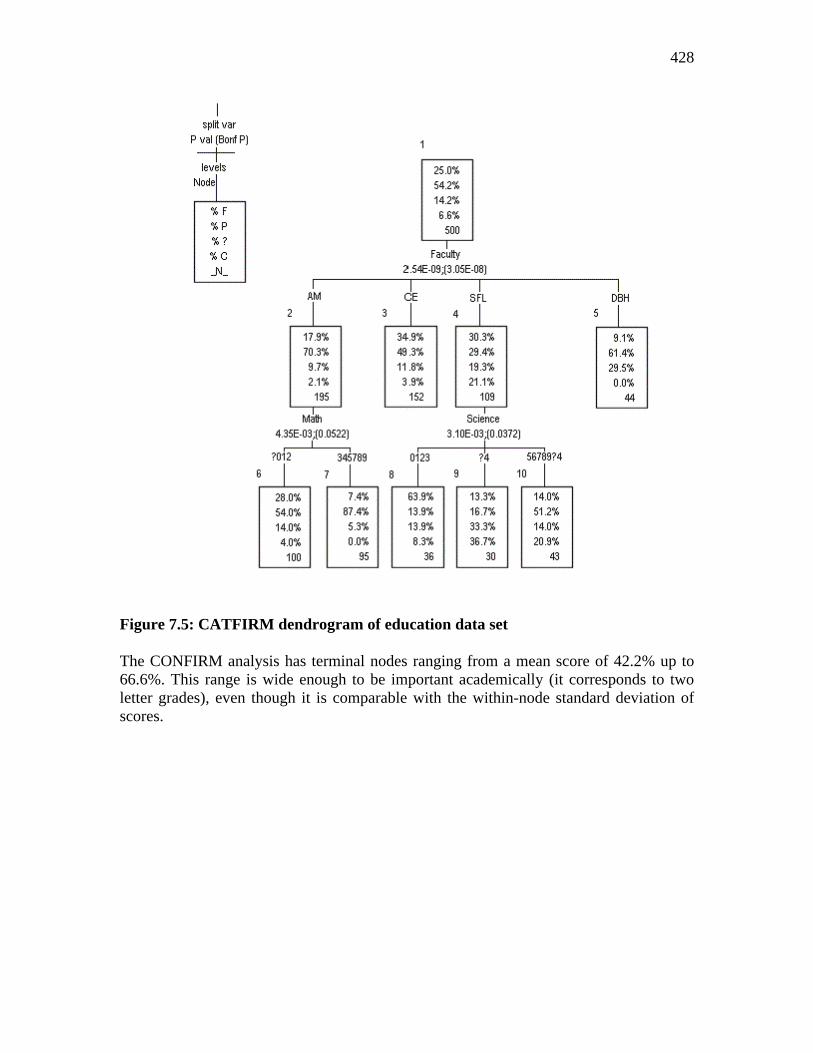
428

Figure 7.5: CATFIRM dendrogram of education data set The CONFIRM analysis has terminal nodes ranging from a mean score of 42.2% up to 66.6%. This range is wide enough to be important academically (it corresponds to two letter grades), even though it is comparable with the within-node standard deviation of scores.

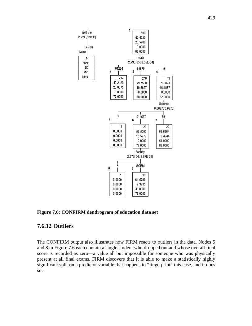
429

Figure 7.6: CONFIRM dendrogram of education data set

7.6.12 Outliers

The CONFIRM output also illustrates how FIRM reacts to outliers in the data. Nodes 5 and 8 in Figure 7.6 each contain a single student who dropped out and whose overall final score is recorded as zero—a value all but impossible for someone who was physically present at all final exams. FIRM discovers that it is able to make a statistically highly significant split on a predictor variable that happens to “fingerprint” this case, and it does so.

430

7.6.13 Overall Method of Operation

CONFIRM with a categorical (free) predictor is like a one-way analysis of variance on that predictor, except that CONFIRM groups together different predictor classes that seem not to differ significantly. CONFIRM for an ordinal predictor is a possible alternative to linear regression, with the difference that while linear regression assumes a constant rate of increase as you go from one level of the ordinal predictor to another, CONFIRM uses a “staircase” model where the dependent variable either remains constant as you go from one level to the next, or jumps by some (not necessarily constant) amount.

Most other recursive partitioning procedures fix the number of ways a node splits, commonly considering only binary splits. FIRM’s method of reducing the classes of the predictors differs from these approaches. A c-category predictor may group into any of 1 through c categories, the software deciding what level of grouping the data appear to require. Both CONFIRM and CATFIRM follow the same overall approach. If a predictor has c classes, the cases are first split into c separate groups corresponding to these classes. Then tests are carried out to see whether these classes can be reduced to fewer classes by pooling classes pairwise. This is done by finding two-sample test statistics (Student’s t for CONFIRM, chi-squared for CATFIRM) between each pair of classes that could legally be grouped together. The groups that can “legally” be joined depend on the predictor type: • For a free predictor and a character predictor, any two groups can be joined. • For a monotonic predictor, only adjacent groups may be joined. • For a float predictor, any pair of adjacent groups can be joined. In addition, the

floating category can join any other group. • A real predictor works like a monotonic predictor if it has no missing information. If

it is missing on some cases, then it works like a float predictor. If the most similar pair fails to be significantly different at the user-selected significance level, then the two classes are merged into one composite class, reducing the number of groups by 1. The pairwise tests are then repeated for the reduced set of c - 1 classes. This process continues until no legally poolable pair of simple or composite classes is separated by a non-significant test statistic, ending the “merge” phase of the analysis. Let’s illustrate this process with CONFIRM’s handling of the floating predictor EMV in the “head injuries” data. The process starts with the following overall summary statistics for the grouping of the cases by EMV:

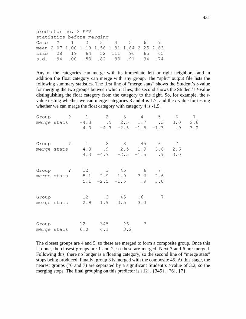
431

predictor no. 2 EMV statistics before merging Cate ? 1 2 3 4 5 6 7 mean 2.07 1.00 1.19 1.58 1.81 1.84 2.25 2.63 size 28 19 64 52 111 96 65 65 s.d. .94 .00 .53 .82 .93 .91 .94 .74

Any of the categories can merge with its immediate left or right neighbors, and in addition the float category can merge with any group. The “split” output file lists the following summary statistics. The first line of “merge stats” shows the Student’s t-value for merging the two groups between which it lies; the second shows the Student’s t-value distinguishing the float category from the category to the right. So, for example, the t-value testing whether we can merge categories 3 and 4 is 1.7; and the t-value for testing whether we can merge the float category with category 4 is -1.5. Group ? 1 2 3 4 5 6 7 merge stats -4.3 .9 2.5 1.7 .3 3.0 2.6 4.3 -4.7 -2.5 -1.5 -1.3 .9 3.0

Group ? 1 2 3 45 6 7 merge stats -4.3 .9 2.5 1.9 3.6 2.6 4.3 -4.7 -2.5 -1.5 .9 3.0

Group ? 12 3 45 6 7 merge stats -5.1 2.9 1.9 3.6 2.6 5.1 -2.5 -1.5 .9 3.0

Group 12 3 45 ?6 7 merge stats 2.9 1.9 3.5 3.3

Group 12 345 ?6 7 merge stats 6.0 4.1 3.2

The closest groups are 4 and 5, so these are merged to form a composite group. Once this is done, the closest groups are 1 and 2, so these are merged. Next ? and 6 are merged. Following this, there no longer is a floating category, so the second line of “merge stats” stops being produced. Finally, group 3 is merged with the composite 45. At this stage, the nearest groups (?6 and 7) are separated by a significant Student’s t-value of 3.2, so the merging stops. The final grouping on this predictor is {12}, {345}, {?6}, {7}.

432

To protect against occasional bad groupings formed by this incremental approach, FIRM can test each composite class of three or more categories to see whether it can be resplit into two that are significantly different at the split significance level set for the run. If this occurs, then the composite group is split and FIRM repeats the merging tests for the new set of classes. This split test is not needed very often, and can be switched off to save execution time by specifying a split significance level that is smaller than the merge significance level.

The end result of this repeated testing is a grouping of cases by the predictor. All classes may be pooled into one, indicating that that predictor has no descriptive power in that node. Otherwise, the analysis ends with from 2 to c composite groups of classes, with no further merging or splitting possible without violating the significance levels set.

The last part of the FIRM analysis of a particular predictor is to find a formal significance level for it. In doing this, it is essential to use significance levels that reflect the grouping of categories that has occurred between the original c-way split and the final (say k-way) split. Hawkins and Kass (1982) mention two ways of measuring the overall significance of a predictor conservatively—the “Bonferroni” approach, and the “Multiple comparison” approach. Both compute an overall test statistic of the k-way classification: for CATFIRM a Pearson 2χ -statistic, and for CONFIRM a one-way analysis of variance F-ratio. The Bonferroni approach takes the p-value of the resulting test statistic and multiplies it by the number of implicit tests in the grouping from c categories to k. There are two possible multiple comparison p-values. The default in (versions of FIRM through FIRM 2.0) computes the p-value of the final grouping as if its test statistic had been based on a c-way classification of the cases. The default introduced in FIRM 2.1 is the p-value of the original c-way classification, but the earlier multiple comparison test can be selected if desired. Since both the Bonferroni and multiple comparison approaches yield conservative bounds on the p-value, the smaller of the two values is taken to be the overall significance of the predictor.

The final stage is the decision of whether to split the node further and, if so, on which predictor. FIRM does this by finding the most significant predictor on the conservative test, and making the split if its conservative significance level multiplied by the number of active predictors in the node is below the user-selected cutoff. The FIRM analysis stops when none of the nodes has a significant split.

Some users prefer not to split further any nodes that contain only a few, or very homogeneous, cases. Some wish to limit the analysis to a set maximum number of nodes. The codes contain options for these preferences, allowing the user to specify threshold sizes (both codes) and a threshold total sum of squares (CONFIRM) that a node must

433

have to be considered for further splitting, and to set a maximum number of nodes to be analyzed.

7.6.14 Comparison with Other Codes

Before discussing the details of using the codes, we mention some historical development and other related approaches. The original source on recursive partitioning was the work of Morgan and Sonquist (1963) and their “Automatic Interaction Detector” (AID). This covered monotonic and free predictors, and made only binary splits. At each node, the split was made where the explained sum of squares was greatest, and the analysis terminated when all remaining nodes had sums of squared deviations below some user-set threshold. It was soon found that the lack of a formal basis for stopping made the procedure prone to overfitting. In addition, the use of explained sum of squares without any modification for the number of starting classes or the freedom to pool them also made AID tend to prefer predictors with many categories to those with fewer, and to prefer free predictors to monotonic. Breiman et al (1984) built on the AID foundation with their Classification and Regression Trees approach. This has two classes of predictors—categorical (corresponding to AID’s “free” predictors) and continuous; unlike FIRM, their method does not first reduce continuous (in FIRM terminology “real”) predictors down to a smaller number of classes, nor does it draw any distinction between these and monotonic predictors with just a few values. The Breiman et al methodology does not have an equivalent to our “floating” category. Instead, missing values of predictors are handled by “surrogate splits”, by which when a predictor is missing on some case, other predictors are used in its stead. This approach depends on the predictive power of the missingness being captured in other non-missing predictors. Breiman et al use only binary splits. Where FIRM chooses between different predictors on the basis of a formal test statistic for identity, they use a measure of “node purity”, with the predictor giving the purest descendant nodes being the one considered for use in splitting. This leads to a tendency to prefer categorical predictors to continuous, and to prefer predictors with many distinct values to predictors with few. FIRM’s use of conservative testing tends to lead to the opposite biases, since having more categories, or being free rather than monotonic, increases the Bonferroni multipliers applied to the predictor’s raw significance level. With a continuous dependent variable, their measure of node purity comes down to essentially a two-sample t (which FIRM would also use for a binary split), but their purity measure for a categorical dependent variable is very different than FIRM’s. FIRM looks for statistically significant differences between groups while they look for splits that will classify to different classes. So the Breiman et al approach seeks two-column cross

434

classifications with different modal classes—that is, in which one category of the dependent variable has the largest frequency in one class while a different category has the largest frequency in the other class. FIRM looks instead for groupings that give large chi-squared values, which will not necessarily have different modal classes. This important difference has implications for the use of the two procedures in minimal-model classification problems. As it is looking for strong relationships rather than good classification rules, a FIRM analysis may produce a highly significant split, but into a set of nodes all of which are modal for the same class of the dependent variable. An example of this is the split of Node 4 of the head injuries data set (Figure 7.3). This creates two descendant nodes with 52% and 86% moderate to good recoveries. If all you care about is predicting whether a patient will make a moderate to good recovery, this split is pointless—in both descendant nodes you would predict a moderate to good recovery. But if you want to explore the relationship between the indicator and the outcome, this split would be valuable, as the proportions of favorable outcomes are substantially different. It might also be that a clinician might treat two patients differently if it is known one of them has a 86% chance of recovery while the other has a 52% chance, even though both are expected to recover. In this case, too, the FIRM split of the node could provide useful information.

Two major differences between FIRM and the Classification and Regression Trees method relate to the rules that are used to decide on the final size of tree. FIRM creates its trees by “forward selection”. This means that as soon as the algorithm is unable to find a node that can be split in a statistically significant way, the analysis stops. Since it is possible for a non-explanatory split to be needed before a highly explanatory one can be found at a lower level, it is possible for the FIRM analysis to stop too soon and fail to find all the explanatory power in the predictors. It is easy to construct artificial data sets in which this happens. You can protect yourself against this eventuality by initially running FIRM with a lax splitting criterion to see if any highly significant splits are hidden below non-significant ones; if not, then just prune away the unwanted non-significant branches of the dendrogram. Particularly when using the printed dendrogram, this is a very easy operation as all the splits are labeled with their conservative significance level. We do not therefore see this theoretical possibility of stopping too soon as a major practical weakness of FIRM’s forward testing approach. Breiman et al use the opposite strategy of “backward elimination”. First, a deliberately very oversized tree is created by continuing to split nodes, whether the splits produce some immediate benefit or not. Then the oversized tree is pruned from the bottom, undoing splits that appear not to correspond to distinct patterns in the data.

435

The second, more profound difference is in the procedure used to decide whether a particular split is real, or simply a result of random sampling fluctuations giving the appearance of an explanatory split. FIRM addresses this issue using the Neyman Pearson approach to hypothesis testing. At each node, there is a null hypothesis that the node is homogeneous, and this is tested using a controlled, conservative significance level. In the most widely-used option, Breiman et al decide on the value of a split using cross validation. We will do no more than sketch the implications, as the method is complicated (see for example Breiman, et al, 1984 or McLachlan, 1992). An original very oversized tree is formed. The sample is then repeatedly (typically 10 times) split into a “calibration” subsample and a “holdback” sample. The same tree analysis is repeated on the calibration subsample as was applied to the full data and this tree is then applied to the holdback sample, to get an “honest” measure of its error rate. The picture obtained from these 10 measures is then used to decide how much of the detail of the original tree was real and how much due just to random sampling effects. This leads to a pruning of the original tree, cutting away all detail that fails to survive the cross-validation test. As this sketch should make clear, an analysis using the Breiman et al methodology generally involves far more computing than a FIRM analysis of the same data set. As regards stopping rules, practical experience with the two approaches used for a continuous dependent variable seems to be that in data sets with strong relationships, they tend to produce trees of similar size and form. In data sets with weak, albeit highly significant relationships, FIRM’s trees appear to be generally larger and more detailed. See Hawkins and McKenzie (1995) for some further examples and discussion of relative tree sizes of the two methods. In view of the very different objectives of the two approaches to analysis of categorical data (getting classification rules and uncovering relationships respectively), there are probably few useful general truths about the relative performance of the two approaches for a categorical dependent variable. Another recursive partitioning method is the Fast Algorithm for Classification Trees (FACT), of Loh and Vanichsetakul (1988). This method was designed for a categorical dependent variable, and treats the splitting by using a discriminant analysis paradigm. The KnowledgeSEEKER procedure is also based on the CHAID algorithm and produces results similar to those of CATFIRM. The main technical difference from FIRM (other than the more user-friendly interface) lies in the conservative bounds used to assess a predictor, where KnowledgeSEEKER uses a smaller Bonferroni multiplier than does FIRM. The public domain SAS procedure TREEDISC (available on request by Warren Sarle of SAS Institute) also implements an inference-based approach to recursive partitioning. The SAS Data Mining module also contains a variety of RP approaches including all three widely-used approaches.

436

This list is far from exhaustive—there are many other RP approaches in the artificial intelligence arena—but perhaps covers some of the major distinct approaches.

7.7 Graphical Display of Data

Graphics are often a useful data-exploring technique through which the researcher may familiarize her or himself with the data. Relationships and trends may be conveyed in an informal and simplified visual form via graphical displays. In addition to the display of a bar chart, histogram, 3-D bar chart, line and bivariate scatter plot, LISREL 8.50 for Windows now includes options to display a pie chart, box-and-whisker plot and a scatter plot matrix. By opening a PRELIS system file (see Section 7.1 and Chapter 2), the PSF toolbar appears and one may select either of the Univariate, Bivariate or Multivariate options from the Graphs menu.

7.7.1 Pie Chart

A pie chart display of the percentage distribution of a variable is obtained provided that

• The variable is defined as ordinal. Variables types are defined via the Data, Define Variables option.

• The variable does not have more than 15 distinct values. Pie charts may be customized by using the graph editing dialog boxes discussed in Chapter 2. The pie chart below is obtained by opening the dataset income.psf from the mlevelex folder. Select the Graphs, Univariate option to go to the Univariate Plots dialog box. Select the variable group and click the Pie Chart radio button.

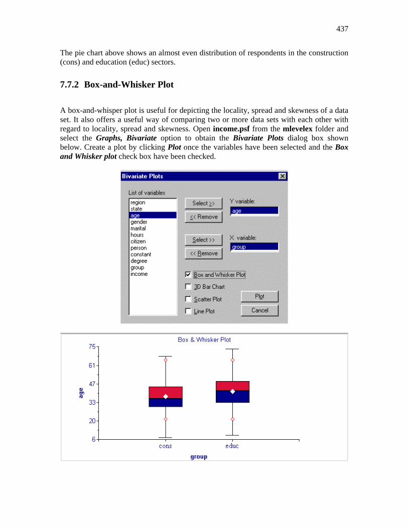
437

The pie chart above shows an almost even distribution of respondents in the construction (cons) and education (educ) sectors.

7.7.2 Box-and-Whisker Plot

A box-and-whisper plot is useful for depicting the locality, spread and skewness of a data set. It also offers a useful way of comparing two or more data sets with each other with regard to locality, spread and skewness. Open income.psf from the mlevelex folder and select the Graphs, Bivariate option to obtain the Bivariate Plots dialog box shown below. Create a plot by clicking Plot once the variables have been selected and the Box and Whisker plot check box have been checked.

438

The bottom line of a box represents the first quartile ( 1q ), the top line the third quartile

( 3q ), and the in-between line the median (me). The arithmetic mean is represented by a

diamond. The whiskers of these boxes extend to 3 11.5( )q q− on both sides of the median. The

length of the whiskers is based on a criterion of Tukey (1977) for determining whether outliers are present. Any data point beyond the end of the whiskers is then considered an outlier. Two red circles are used to indicate the minimum and maximum values. Graph parameters that may be changed include the axes and description thereof, the symbols used and the colors assigned to the symbols/text. To change any of these, simply double-click on the symbol/text to be changed to activate a dialog box in which changes can be requested. For symmetric distributions the mean equals the median and the in-between line divides the box in two equal parts. From the graphics display above we conclude

• The age distribution of respondents from the construction sector are positively skewed while the opposite holds for the education sector.

• The mean age of respondents from the education sector is greater than those from the construction sector.

For a large sample from a normal distribution, the plotted minimum and maximum values should be close to the whiskers of the plot. This is not the case for either of the groups and we conclude that the distribution of age values in this data is not bell-shaped. This observation may be further confirmed by making histogram displays of Age using the datasets cons.psf and educ.psf, these being subsets of the income.psf dataset.

7.7.3 Scatter Plot Matrix

The scatter plot matrix, as implemented in LISREL, provides an organized way of simultaneously looking at bivariate plots of up to ten variables. Except for the diagonal, each frame contains a scatter plot. The diagonals contain the variable names and the minimum and maximum values of the corresponding variables. Each scatterplot is a visual summary of linearity, nonlinearity, and separated points (see, for example, Cook and Weisberg (1994)). Select Open from the File menu and select the PRELIS system file fitchol.psf from the tutorial folder.

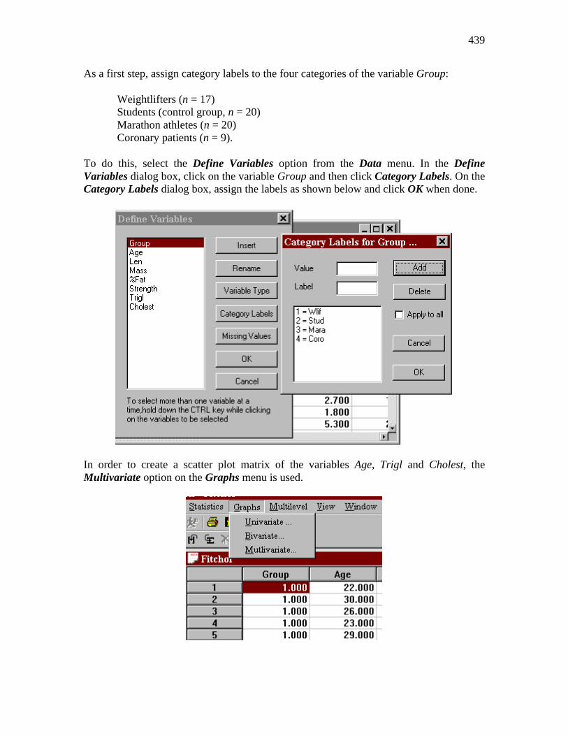
439

As a first step, assign category labels to the four categories of the variable Group:

Weightlifters (n = 17) Students (control group, n = 20) Marathon athletes (n = 20) Coronary patients (n = 9).

To do this, select the Define Variables option from the Data menu. In the Define Variables dialog box, click on the variable Group and then click Category Labels. On the Category Labels dialog box, assign the labels as shown below and click OK when done.

In order to create a scatter plot matrix of the variables Age, Trigl and Cholest, the Multivariate option on the Graphs menu is used.

440

As a result, the Scatter Plot Matrix dialog box appears. The variables Age, Trigl and Cholest are selected and added to the Selected window. The variable Group, representing the four groups to which we have just assigned category labels, is added to the Mark by window. Click Plot to create the 3 x 3 scatter plot matrix.

The scatter plot matrix is shown below. In the first row of plots at the top of the matrix, Cholest is plotted against Age and Trigl respectively. The third plot in this row contains the variable name and the observed minimum and maximum values of Cholest. The first plot in the second row shows the scatter plot of Trigl against Age. The other scatter plots are essentially mirror images of the three discussed this far and are the plots for (Cholest, Trigl), (Trigl, Age) and (Cholest, Age) respectively. The diagonal elements of the matrix contain the names, minimum and maximum values of each variable. From the display, it is apparent that the (Age, Trigl) and (Age, Cholest) scatter plots of coronary patients, denoted by a “+” symbol, are clustered together, away from the main cluster of points formed by the other three groups. In the (Age, Age) segment the minimum and maximum values of the Age variable are given.

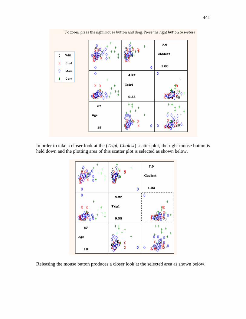
441

In order to take a closer look at the (Trigl, Cholest) scatter plot, the right mouse button is held down and the plotting area of this scatter plot is selected as shown below.

Releasing the mouse button produces a closer look at the selected area as shown below.

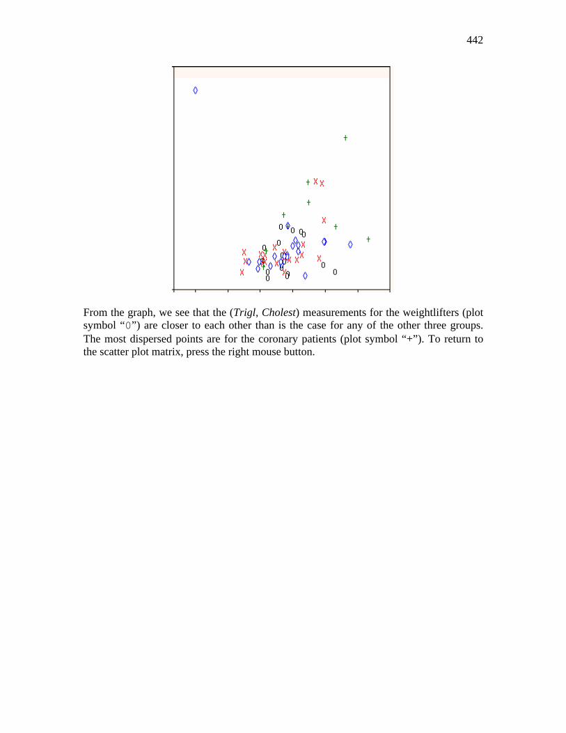
442

From the graph, we see that the (Trigl, Cholest) measurements for the weightlifters (plot symbol “0”) are closer to each other than is the case for any of the other three groups. The most dispersed points are for the coronary patients (plot symbol “+”). To return to the scatter plot matrix, press the right mouse button.