Embed Size (px)
Citation preview

Lecture slides by Kevin WayneCopyright © 2005 Pearson-Addison Wesley
http://www.cs.princeton.edu/~wayne/kleinberg-tardos
Last updated on 4/17/18 9:07 AM
7. NETWORK FLOW I
‣ Ford–Fulkerson demo
‣ exponential-time example
‣ pathological example

7. NETWORK FLOW I
‣ Ford–Fulkerson demo
‣ exponential-time example
‣ pathological example
SECTION 7.1

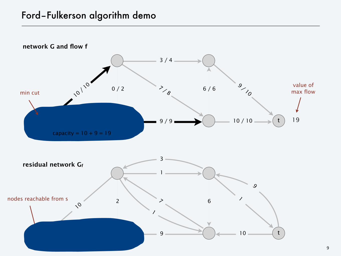
Ford–Fulkerson algorithm demo
3
s t
0 / 20 /
10 0 / 6
0 / 10
0 / 4
0 / 8
0 / 9
network G and flow f
0 / 10 0
value of flow
0 / 10
flow capacity
s t
2 6
10
4
9
residual network Gf
10
residual capacity
10 10 8

Ford–Fulkerson algorithm demo
4
2 6
4
9
residual network Gf
10
10
s t
0 / 20 /
10 0 / 6
0 / 10
0 / 4
0 / 8
0 / 9
network G and flow f
0 / 10 0
0 / 10
s t
10
10
8
8—
8—
8—
+ 8 = 8

Ford–Fulkerson algorithm demo
5
4residual network Gf
10
s t
0 / 28 /
10 0 / 6
8 / 10
0 / 4
8 / 8
0 / 9
network G and flow f
0 / 10 8
0 / 10
8
8
8
9s
22
—10 2 —
2— + 2 = 10
10 6
10—
2 t

Ford–Fulkerson algorithm demo
6
4residual network Gf
s t
2 / 210 /
100 / 6
10 / 10
0 / 4
8 / 8
2 / 9
network G and flow f
0 / 10 10
0 / 10
8
2
2
10
10
10 7s
10 6
t
6 —
8—
6— + 6 = 16
6—

Ford–Fulkerson algorithm demo
7
residual network Gf
s t
2 / 210 /
106 / 6
10 / 10
0 / 4
8 / 8
8 / 9
network G and flow f
6 / 10 16
6 / 10
8
8
10
10
1
6
6
6
4
4s
4
t
2
8—
0 —
2—
8—
+ 2 = 18
fixes mistake from second augmenting path

Ford–Fulkerson algorithm demo
8
residual network Gf
s t
0 / 210 /
106 / 6
10 / 10
2 / 4
8 / 8
8 / 9
network G and flow f
8 / 10 18
8 / 10
8
10
10 6
8
2
2
8
1
2
s
2
t2
8
9—
9—
7—
3—
9—
+ 1 = 19
Ford–Fulkerson algorithm demo
9
residual network Gf
s t
0 / 210 /
106 / 6
10 / 10
3 / 4
7 / 8
9 / 9
network G and flow f
9 / 10 19
9 / 10
10
10 6
9
2
3
9
9
1
s
1
t1
7
1
nodes reachable from s
min cutvalue of max flow
capacity = 10 + 9 = 19

7. NETWORK FLOW I
‣ Ford–Fulkerson demo
‣ exponential-time example
‣ pathological example
SECTION 7.1

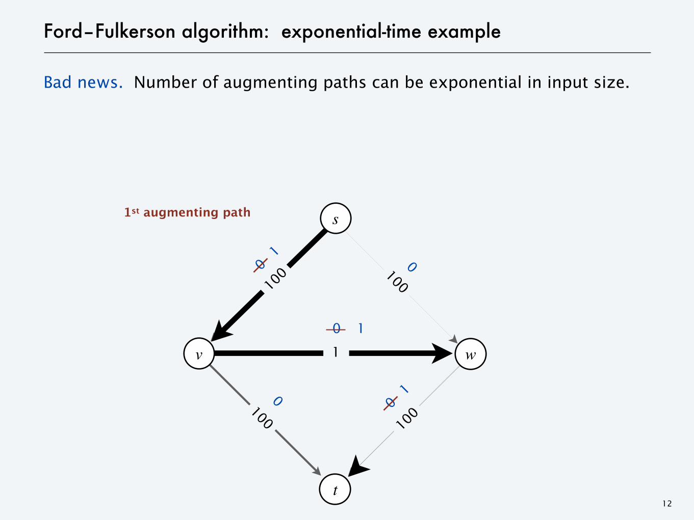
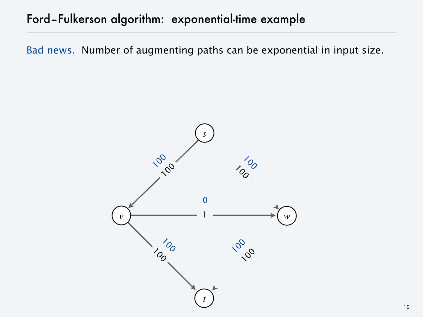
Ford–Fulkerson algorithm: exponential-time example
Bad news. Number of augmenting paths can be exponential in input size.
11
v w
t
s
0
1
00
0capacity
flow
100
100
100
100
0
initialize with 0 flow
Ford–Fulkerson algorithm: exponential-time example
Bad news. Number of augmenting paths can be exponential in input size.
12
0
00
1
0
0
1st augmenting path
1
1
1
100
100
100
100
t
s
v w

Ford–Fulkerson algorithm: exponential-time example
Bad news. Number of augmenting paths can be exponential in input size.
13
1
1
1
2nd augmenting path
0
0
1
1
1
0
100
100
100
100
t
s
v w

Ford–Fulkerson algorithm: exponential-time example
Bad news. Number of augmenting paths can be exponential in input size.
14
1
11
1
1
0
3rd augmenting path
2
2
1
100
100
100
100
t
s
v w

Ford–Fulkerson algorithm: exponential-time example
Bad news. Number of augmenting paths can be exponential in input size.
15
2
2
1
4th augmenting path
1
1
1
2
2
0
100
100
100
100
t
s
v w
Ford–Fulkerson algorithm: exponential-time example
Bad news. Number of augmenting paths can be exponential in input size.
16
. . .

Ford–Fulkerson algorithm: exponential-time example
Bad news. Number of augmenting paths can be exponential in input size.
17
99
1
99
0
199th augmenting path
100
100
1
99
99
100
100
100
100
t
s
v w

Ford–Fulkerson algorithm: exponential-time example
Bad news. Number of augmenting paths can be exponential in input size.
18
100
100
1
200th augmenting path
99
99
1
100
100
0
100
100
100
100
t
s
v w
Ford–Fulkerson algorithm: exponential-time example
Bad news. Number of augmenting paths can be exponential in input size.
19
0
100
100
1
100
100
100
10010
0
100
t
s
v w
7. NETWORK FLOW I
‣ Ford–Fulkerson demo
‣ exponential-time example
‣ pathological example
SECTION 7.1

Ford–Fulkerson algorithm: pathological example
Intuition. Let r > 0 satisfy r2 = 1 – r.
・Initially, some residual capacities are 1 and r.
・After two augmenting paths, some residual capacities are r and r2.
・After two more augmenting paths, some residual capacities are r2 and r3.
・After two more, some residual capacities are r3 and r4.
・By carefully choreographing the augmenting paths,infinitely many residual capacities arise!
21
1 – r
r – r2
r2 – r3
r =
�5 � 1
2=� r2 = 1 � r
r � 0.618 =� r4 < r3 < r2 < r < 1

Ford–Fulkerson algorithm: pathological example
22
v
u
w
xs 0 / C
0 / C 0 / r
0 / 1
0 / 1
t
0 / C
0 / C
0 / C
0 / Cw
x
v
us
t
C sufficiently large that it won’t ever be a bottleneck (we'll suppress)
flow network G
r =
�5 � 1
2=� r2 = 1 � r

Ford–Fulkerson algorithm: pathological example
23
v
u
w
xs
0 / r
augmenting path 1: s→w→v→t (bottleneck capacity = 1)
0 / 1
t
w
x
v
us
t
0 / 1—
1
r =
�5 � 1
2=� r2 = 1 � r

Ford–Fulkerson algorithm: pathological example
24
v
u
w
xs
augmenting path 2: s→u→v→w→x→t (bottleneck capacity = r)
t
w
x
v
us
t
0 / r
0 / 1
1 / 1—
1 – r
—r = 1
– r2
—r
r =
�5 � 1
2=� r2 = 1 � r

Ford–Fulkerson algorithm: pathological example
25
v
u
w
xs
augmenting path 3: s→w→v→u→t (bottleneck capacity = r)
t
w
x
v
us
t
r / r
1 – r
2 / 1
1 – r / 1
1
—
0
r =
�5 � 1
2=� r2 = 1 � r

Ford–Fulkerson algorithm: pathological example
26
v
u
w
xs
augmenting path 4: s→u→v→w→x→t (bottleneck capacity = r2)
t
w
x
v
us
t
0 / r
1 / 1—
1 – r2
—r2 =
r – r3
1 – r
2 / 1
1
r =
�5 � 1
2=� r2 = 1 � r
Ford–Fulkerson algorithm: pathological example
27
v
u
w
xs
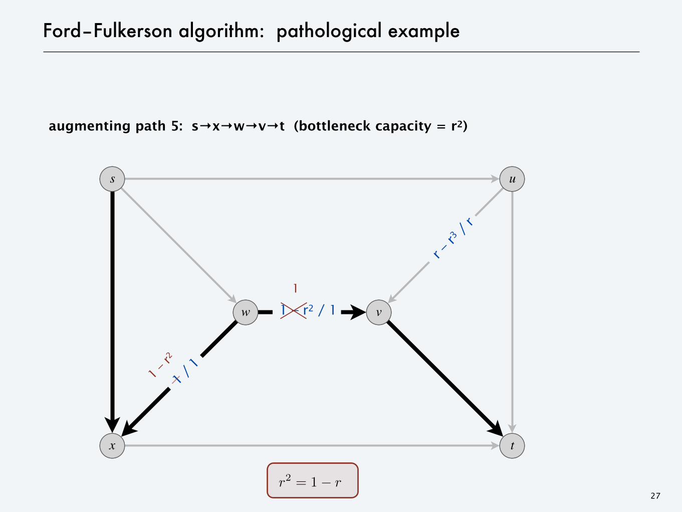
augmenting path 5: s→x→w→v→t (bottleneck capacity = r2)
t
w
x
v
us
t
1 / 1
1 – r2 / 1
—1 – r
2
1
r – r3 /
r
r =
�5 � 1
2=� r2 = 1 � r

Ford–Fulkerson algorithm: pathological example
28
v
u
w
xs
augmenting path 6: s→u→v→w→x→t (bottleneck capacity = r3)
t
w
x
v
us
t
1 – r
2 / 1
1 / 1—
1 – r3
1 – r
2 + r3 =
1 –
r4
r – r3 /
rr
r =
�5 � 1
2=� r2 = 1 � r

Ford–Fulkerson algorithm: pathological example
29
v
u
w
xs
augmenting path 7: s→w→v→u→t (bottleneck capacity = r3)
t
w
x
v
us
t
r / r
1 – r3 / 1
1
—r –
r3
1 – r
4 / 1
r =
�5 � 1
2=� r2 = 1 � r
Ford–Fulkerson algorithm: pathological example
30
v
u
w
xs
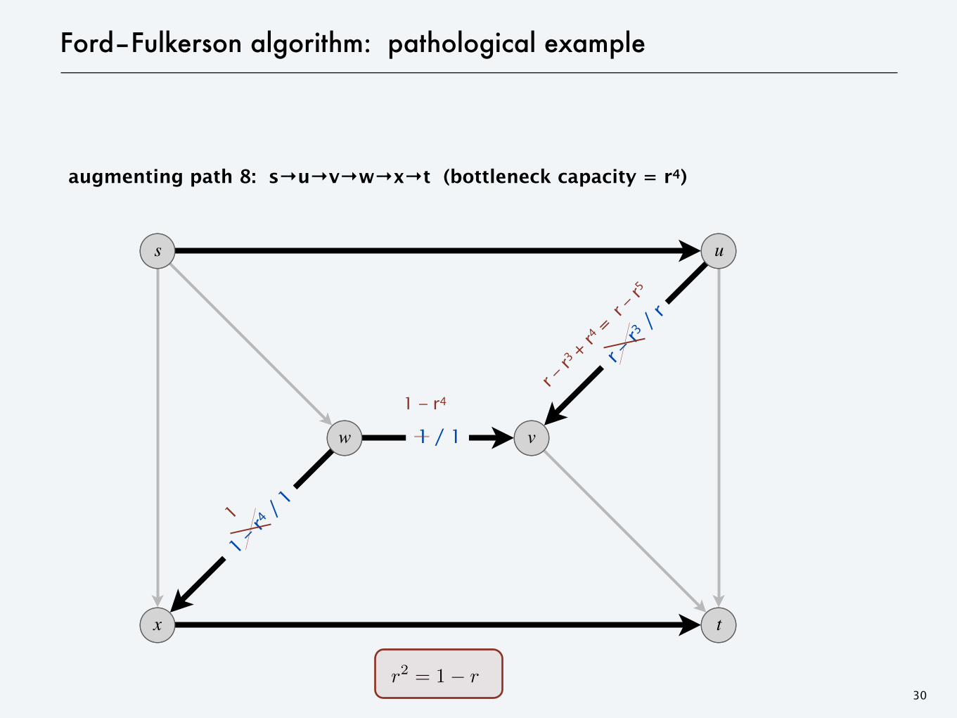
augmenting path 8: s→u→v→w→x→t (bottleneck capacity = r4)
t
w
x
v
us
t
r – r3 /
r
1 / 1—
1 – r4
1
1 – r
4 / 1
r – r3 +
r4 =
r –
r5
r =
�5 � 1
2=� r2 = 1 � r

Ford–Fulkerson algorithm: pathological example
31
v
u
w
xs
augmenting path 9: s→x→w→v→t (bottleneck capacity = r4)
t
w
x
v
us
t
1 / 1
—1
– r4
1
1 – r4 / 1
r – r5 /
r
r =
�5 � 1
2=� r2 = 1 � r

Ford–Fulkerson algorithm: pathological example
32
v
u
w
xs
flow after augmenting path 5: { r - r3, 1, 1 - r2 } (value of flow = 1 + 2r + 2r2)
t
w
x
v
us
t
1 / 1
flow after augmenting path 1: { r - r1, 1, 1 - r0 } (value of flow = 1)
1 – r
4 / 1
r – r5 /
r
flow after augmenting path 9: { r - r5, 1, 1 - r4 } (value of flow = 1 + 2r + 2r2 + 2r3 + 2r4)
r =
�5 � 1
2=� r2 = 1 � r

Ford–Fulkerson algorithm: pathological example
Theorem. The Ford–Fulkerson algorithm may not terminate; moreover, it
may converge to a value not equal to the value of the maximum flow.
Pf.
・After (1 + 4k) augmenting paths of the form just described,the value of the flow
・Value of maximum flow = 2C + 1. ▪
33
= 1 + 22k�i=1
ri
� 1 + 2��
i=1ri
= 3 + 2r
< 5
= 1 + 22k�i=1
ri
� 1 + 2��
i=1ri
= 3 + 2r
< 5
= 1 + 22k�i=1
ri
� 1 + 2��
i=1ri
= 3 + 2r
< 5
r =
�5 � 1
2=� r2 = 1 � r
= 1 + 22k�i=1
ri
� 1 + 2��
i=1ri
= 1 +2r
1 � r
= 3 + 2r
< 5<latexit sha1_base64="jYbj/lj4jSjHk8u6NuvwVdAASIE=">AAAC+nicbVFNb9QwEHXCVwkf3ZYjF4sVCAmxihdKe6BSJS4ci8S2ldbpynEmW2ttJ7Id1Cjkz3BDXPkhXPk3OGmEutuONNbTm3kz9nNaSmFdHP8Nwjt3791/sPUwevT4ydPt0c7uiS0qw2HGC1mYs5RZkELDzAkn4aw0wFQq4TRdferqp9/AWFHor64uIVFsqUUuOHOeWoz+0BSWQjfMGFa3jeSyjfArfOiT4Dd4iqmtFJVCCWcXjTgk7XkzXbXYnAtK52SyByrpBFSCP2/V+GGdigqdu7pX4jXp/2U0yw3jzdS0DXlr2r7res+7brjp6Mn+wH/0uRdR0NnwgmgxGseTuA98E5ABjNEQx4udYJdmBa8UaMcls3ZO4tIlfp4TXEIb0cpCyfiKLWHuoWYKbNL01rf4pWcynBfGp3a4Z68rGqasrVXqOxVzF3az1pG31eaVyw+SRuiycqD51aK8ktgVuPtHnAkD3MnaA8aN8HfF/IJ5/5z/7bUt/ewS+NpLmstKC15ksMFKd+kMa72LZNOzm+BkOiHxhHx5Pz46GPzcQs/RC/QaEbSPjtBndIxmiAcfAhpAkIffwx/hz/DXVWsYDJpnaC3C3/8A/wXkvg==</latexit><latexit sha1_base64="jYbj/lj4jSjHk8u6NuvwVdAASIE=">AAAC+nicbVFNb9QwEHXCVwkf3ZYjF4sVCAmxihdKe6BSJS4ci8S2ldbpynEmW2ttJ7Id1Cjkz3BDXPkhXPk3OGmEutuONNbTm3kz9nNaSmFdHP8Nwjt3791/sPUwevT4ydPt0c7uiS0qw2HGC1mYs5RZkELDzAkn4aw0wFQq4TRdferqp9/AWFHor64uIVFsqUUuOHOeWoz+0BSWQjfMGFa3jeSyjfArfOiT4Dd4iqmtFJVCCWcXjTgk7XkzXbXYnAtK52SyByrpBFSCP2/V+GGdigqdu7pX4jXp/2U0yw3jzdS0DXlr2r7res+7brjp6Mn+wH/0uRdR0NnwgmgxGseTuA98E5ABjNEQx4udYJdmBa8UaMcls3ZO4tIlfp4TXEIb0cpCyfiKLWHuoWYKbNL01rf4pWcynBfGp3a4Z68rGqasrVXqOxVzF3az1pG31eaVyw+SRuiycqD51aK8ktgVuPtHnAkD3MnaA8aN8HfF/IJ5/5z/7bUt/ewS+NpLmstKC15ksMFKd+kMa72LZNOzm+BkOiHxhHx5Pz46GPzcQs/RC/QaEbSPjtBndIxmiAcfAhpAkIffwx/hz/DXVWsYDJpnaC3C3/8A/wXkvg==</latexit><latexit sha1_base64="jYbj/lj4jSjHk8u6NuvwVdAASIE=">AAAC+nicbVFNb9QwEHXCVwkf3ZYjF4sVCAmxihdKe6BSJS4ci8S2ldbpynEmW2ttJ7Id1Cjkz3BDXPkhXPk3OGmEutuONNbTm3kz9nNaSmFdHP8Nwjt3791/sPUwevT4ydPt0c7uiS0qw2HGC1mYs5RZkELDzAkn4aw0wFQq4TRdferqp9/AWFHor64uIVFsqUUuOHOeWoz+0BSWQjfMGFa3jeSyjfArfOiT4Dd4iqmtFJVCCWcXjTgk7XkzXbXYnAtK52SyByrpBFSCP2/V+GGdigqdu7pX4jXp/2U0yw3jzdS0DXlr2r7res+7brjp6Mn+wH/0uRdR0NnwgmgxGseTuA98E5ABjNEQx4udYJdmBa8UaMcls3ZO4tIlfp4TXEIb0cpCyfiKLWHuoWYKbNL01rf4pWcynBfGp3a4Z68rGqasrVXqOxVzF3az1pG31eaVyw+SRuiycqD51aK8ktgVuPtHnAkD3MnaA8aN8HfF/IJ5/5z/7bUt/ewS+NpLmstKC15ksMFKd+kMa72LZNOzm+BkOiHxhHx5Pz46GPzcQs/RC/QaEbSPjtBndIxmiAcfAhpAkIffwx/hz/DXVWsYDJpnaC3C3/8A/wXkvg==</latexit><latexit sha1_base64="jYbj/lj4jSjHk8u6NuvwVdAASIE=">AAAC+nicbVFNb9QwEHXCVwkf3ZYjF4sVCAmxihdKe6BSJS4ci8S2ldbpynEmW2ttJ7Id1Cjkz3BDXPkhXPk3OGmEutuONNbTm3kz9nNaSmFdHP8Nwjt3791/sPUwevT4ydPt0c7uiS0qw2HGC1mYs5RZkELDzAkn4aw0wFQq4TRdferqp9/AWFHor64uIVFsqUUuOHOeWoz+0BSWQjfMGFa3jeSyjfArfOiT4Dd4iqmtFJVCCWcXjTgk7XkzXbXYnAtK52SyByrpBFSCP2/V+GGdigqdu7pX4jXp/2U0yw3jzdS0DXlr2r7res+7brjp6Mn+wH/0uRdR0NnwgmgxGseTuA98E5ABjNEQx4udYJdmBa8UaMcls3ZO4tIlfp4TXEIb0cpCyfiKLWHuoWYKbNL01rf4pWcynBfGp3a4Z68rGqasrVXqOxVzF3az1pG31eaVyw+SRuiycqD51aK8ktgVuPtHnAkD3MnaA8aN8HfF/IJ5/5z/7bUt/ewS+NpLmstKC15ksMFKd+kMa72LZNOzm+BkOiHxhHx5Pz46GPzcQs/RC/QaEbSPjtBndIxmiAcfAhpAkIffwx/hz/DXVWsYDJpnaC3C3/8A/wXkvg==</latexit>

Reference
34
ELSEVIER Theoretical Computer Science 148 ( 1995) 165-I 70
Theoretical Computer Science
Note The smallest networks on which the Ford-Fulkerson
maximum flow procedure may fail to terminate
Uri Zwick’ Department of Computer Science. Tel Aviv University, Rnmat Ah. 69978 Tel Aviv, Israel
Received November I993 Communicated by M. Nivat
Abstract
It is widely known that the Ford-Fulkerson procedure for finding the maximum flow in a network need not terminate if some of the capacities of the network are irrational. Ford and Fulkerson gave as an example a network with 10 vertices and 48 edges on which their procedure may fail to halt. We construct much smaller and simpler networks on which the same may happen. Our smallest network has only 6 vertices and 8 edges. We show that it is the smallest example possible.
1. Introduction
The maximal flow problem is one of the most fundamental combinatorial optimiza- tion problems. The Ford-Fulkerson augmenting paths procedure is perhaps the most basic method devised for solving it and many more advanced algorithms are based on it.
Ford and Fulkerson themselves point out that their procedure need not terminate if the network it is applied on has some irrational capacities. In their book [3], they describe a network with 10 vertices and 48 edges on which this may happen. Their network is quite complicated and most textbooks (see, e.g., [ 1,2,4-6,8]) that describe their procedure do not present it. A variant of their example appears in [7], it has 14 vertices and 28 edges. We are not aware of any simpler example that had appeared in the literature.
In this note we describe three much smaller and simpler networks, on which the Ford-Fulkerson procedure may fail to terminate. The first two networks contain only 6 vertices and 9 edges each. The third network is yet smaller containing only 6 vertices and 8 edges. All three networks are acyclic and planar. The first two are planar and
* Email: [email protected].
0304-3975/95/$09.50 @ 1995 -EElsevier Science B V. All rights reserved SSDI 0304-3975(95)00022-4