Economics 314 Coursebook, 2019 Jeffrey Parker

7 MONEY, INFLATION, GROWTH, AND

CYCLES

Chapter 7 Contents

A. Topics and Tools ............................................................................ 2

B. Money .......................................................................................... 3

What is money? ........................................................................................................... 3

Money supply and money demand ................................................................................. 4

Money as a social institution ......................................................................................... 5

Why don’t the Ramsey and Diamond economies need money? ......................................... 5

Why do real economies need money? .............................................................................. 7

C. Highlights in the History of Money ..................................................... 9

D. Defining Money in Modern Economies ............................................... 11

E. Monetary Policy and the Supply of Money ........................................... 14

Assets and liabilities in a simple monetary system .......................................................... 14

Money, the monetary base, and the money multiplier .................................................... 16

Monetary policy and interest rates ................................................................................ 19

F. Theories of the Demand for Money .................................................... 21

Quantity theory: Money in the classical macro model .................................................... 21

The evolution of money-demand theory ........................................................................ 23

Keynes’s three motives for money demand ..................................................................... 24

The money-demand decision ....................................................................................... 25

Baumol and Tobin’s transactions-demand model .......................................................... 25

Modeling precautionary demand ................................................................................. 28

Is there a speculative demand for money? ...................................................................... 30

An integrated model of money demand ......................................................................... 32

New Keynesian LM curve ........................................................................................... 33

G. Money in Economic Growth Models .................................................. 34

Simple macroeconomics of money and growth ............................................................... 34

Building money into the microfoundations of growth models .......................................... 35

H. The Financial Crisis of 2008–09 ......................................................... 36

Major elements of the crisis .......................................................................................... 36

Downturn .................................................................................................................. 38

Policy alternatives ...................................................................................................... 40

I. Suggestions for Further Reading ........................................................ 41

7 – 2

The nature and history of money ................................................................................. 41

J. Works Cited in Text ....................................................................... 42

A. Topics and Tools

We have now completed half a semester of analysis of macroeconomic models

and we have yet to introduce one of the principal variables of macroeconomics:

money. How did the Ramseys and Diamonds of these worlds buy and sell things with-

out money? What, if not money, did they borrow and lend in order to execute their

precisely calibrated lifetime consumption plans, maintaining their knife-edge balance

on the saddle path?

We answer that question below by demonstrating how the highly artificial assump-

tions of these models freed their occupants from needing money. In doing so we will

explore the reasons why money is needed when we abandon these assumptions. This

leads us to discuss money’s role in modern economies and what physical and virtual

commodities fulfill that role.

The basic definition of money and its role in the economy is standard content in

both introductory and intermediate macroeconomics courses, which means that the

typical reader of Romer’s textbook will have studied this material twice and need no

review. Because you are using Romer at a much earlier stage of your macroeconomics

education, this chapter will provide material that would normally appear in an under-

graduate course textbook.

To summarize the basic theory of money in stark brevity: Money is demanded by

households and firms as the medium with which to accomplish transactions in the

markets for goods, labor, and credit. The supply of money comes from the banking

system. The ability of the private banking system to create monetary assets depends in

part on the amount of “base money” provided by the central bank, which is often un-

der the direct control or indirect influence of the national government. In the short run,

imbalances between the demand for money and its supply are likely to be resolved by

changes in interest rates, but in the long run changes in the general price level most

likely supplant these interest-rate effects. Changes in interest rates affect investment,

consumption, and saving, so monetary conditions may have a substantial impact on

aggregate demand in the short run.

7 – 3

B. Money

As noted above, the basic story of how the monetary system works is one of the

glaring omissions—for our purposes—from Romer’s text. Given his intended audi-

ence of economics graduate students, there is probably no need to cover these basics.

However, since we are using it in an undergraduate context, we cannot take for granted

that everyone is fully up to speed on what money is and the various theories of why

people demand it. This coursebook chapter fills in some basic information about the

monetary system.

We can introduce monetary issues only briefly here. Students who would like to

learn more details about the monetary system and monetary policy should consider

enrolling in Economics 341: Monetary and Fiscal Policy.

What is money?

Everyone “knows” what money is, but putting a precise definition on it can be

tricky. Economists usually define money functionally—by what it does rather than as

a specific commodity or set of commodities. The two most common (and very closely

related) functions of money are means of payment and medium of exchange. An asset is

a means of payment if receiving it from the buyer in a transaction extinguishes all of

the buyer’s obligations to pay for the commodity being purchased. If you handed the

Reed Bookstore $81.75 in bills and coins as payment for brand new copy of Romer’s

text, you owe nothing further and thus the $81.75 was accepted as a means of payment.

While means of payment and medium of exchange are often used interchangeably,

Goodhart (1989) makes a subtle distinction between the two. Suppose that the

bookstore allows you to “buy” the book using your Reed student account. In this case,

the availability of the Reed account functioned as a medium of exchange because it

allowed the transaction to proceed and facilitated the transfer of the book. However,

it did not extinguish your liability for payment because you still owe Reed $81.75, thus

it did not function as a means of payment. When you bring $81.75 to the Reed cashier

window (or transfer money from your bank account to Reed’s) to retire your debt, the

transaction will be complete.

In many, perhaps most, cases the medium of exchange can also be thought of as a

means of payment. However, in cases such as credit purchases it is clear that there is

a distinction and that money would be defined differently depending on whether we

consider it to be only the asset that provides the means of payment function or all assets

that functioned in the less restrictive capacity of medium of exchange.

Money also provides several other functions. The use of money as a means of pay-

ment makes it convenient to quote prices in terms of money—to use money as a unit

7 – 4

of account. Thus the dollar in the United States is not only a physical commodity such

as a bill or coin, but also an abstract unit in which value is measured. The unit of

account and the means of payment need not always be the same. For example, in some

tourist locations or border communities outside the United States prices are quoted in

the local currency but dollars are also accepted as means of payment. Other examples

include international “moneys.” The euro existed as a unit of account for international

transactions among would-be adopters for several years before coins and notes were

issued.

Money also usually serves as a standard of deferred payment, meaning that future

payments are contracted in terms of dollars. Rapid and (particularly) variable inflation

reduces money’s effectives in this role.

Finally, like nearly all other durable assets, money is a store of value. The effective-

ness of an asset as a store of value depends on the degree and certainty with which the

asset maintains its value over time. Money retains its value well as long as inflation is

predictably low and the likelihood of replacement of the current monetary asset

(through political revolution or monetary reform) is remote. When money’s role as a

store of value is compromised (usually through hyperinflation), people will not want

to hold it, hence it will tend to be replaced as a means of payment as well through

currency substitution.

Money supply and money demand

The role of money in the macroeconomy is usually examined in a supply/demand

framework. The supply of money in modern economies is determined by the interac-

tions of the monetary policy authority (central bank) and the financial system (espe-

cially commercial banks). The demand for money depends on the behavior of the house-

holds and firms that hold monetary assets.

Macroeconomists agree on simple models of the money-supply process. The cen-

tral bank conducts monetary policy by controlling the creation of “high-powered

money” (or the monetary base), which can be used in transactions or held in reserve

by depository financial institutions (banks) to back their customers’ deposits. These

deposits at banks perform at least some of the key functions of money, hence are usu-

ally included in the money supply. However, as long as banks hold reserves against

their deposits, the amount of deposit money that banks can create is limited by the

availability of high-powered central-bank money, thus providing the central bank with

a mechanism to control the overall money supply. The process of money creation and

monetary control by the central bank is detailed in Section E below.

In contrast to the simple and effective models of the supply of money, the modeling

of money demand has been a source of great frustration for macroeconomists since

about 1970. Rapid technological progress and regulatory changes have revolutionized

how people use various liquid “money” assets. This has made it difficult to find a stable

7 – 5

sample period over which to test even the most basic propositions about money de-

mand.

Money as a social institution

Most of us have grown up under a stable regime of government-issued “fiat”

money.1

This can make the nature of money seem static and even immutable, but it is

important to remember that money is whatever people accept as means of payment,

so the character of an economy’s money ultimately depends on the behavior of those

people.

At most times in the recent history of most countries, a government has defined a

specific monetary commodity such as dollars, pounds, yen, or euros. These govern-

ment currencies are usually legislated to be “legal tender,” which means that they serve

by law as means of payment, in particular for payments involving government such as

taxes or government purchases.

However, in extreme times such legislated mandates may not be enforced or en-

forceable. In a country whose currency is undergoing extreme inflation—hyperinfla-

tion—people may refuse to hold or accept the country’s currency and instead insist on

payment with either physical commodities (such as gold) or stable foreign currency

(such as U.S. dollars). Hyperinflation in Zimbabwe from 2007 to 2009 led the govern-

ment to abandon printing Zim dollars and admit that the U.S. dollar was the de facto

Zimbabwean currency. Another example is Ecuador, which abandoned the sucre in

2000 during high inflation and a financial crisis.

Ultimately, it is the members of society who, by their willingness to accept it in

exchange, determine what commodity or commodities will serve the role of money.

As long as currency is in common use for exchange the money supply should include

people’s holdings of currency. If personal checks are widely accepted as means of pay-

ment, then checking account balances should be included in one’s holdings of money.

Thus, money is a social construction; money is whatever the members of society rou-

tinely accept as a means of payment. Governments can influence societies’ choice of

monetary assets by providing a stable currency and mandating it as legal tender, but

money is ultimately a social rather than a government institution.

Why don’t the Ramsey and Diamond economies need money?

Exchange is the mechanism through which households and firms buy and sell the

goods, services, and productive resources that give the former utility and income and

the latter revenue and profit. Until now, we have devoted no attention at all to the

1

Fiat money is money that has no intrinsic worth and for which there is no promise of redemp-

tion for something such as gold that has intrinsic worth.

7 – 6

process of exchange. It is rather remarkable that we could reach the midpoint of a mac-

roeconomics course without having discussed money, prices, or inflation. Thinking

about why that has been possible will help us understand the essential role of money

in modern economies.

First, consider the economy of the Ramsey growth model. At moment t each

household produces an amount

A t L t

f k tH

of the generic output good (output per effective labor unit multiplied times the number

of effective labor units in the household). Of these units produced, some are consumed

and some are invested in new capital.

Does this household need to undertake any transactions whatsoever with others?

No. There is only one generic good, so there is no need to trade one’s own apples for

apples produced by others. All households are identical, so there are no households

that are saving while others are dissaving, so there is no need for a credit market,

though we maintain the possibility of one to motivate the idea of saving and dissaving.

This model works in exactly the same way if the economy is one gigantic household

or if it comprises millions of small ones.2

There is no need for exchange, so there is no

need to model the mechanism or technology of exchange and thus no need for money.

The Diamond overlapping-generations model is a bit closer to needing money be-

cause it involves, in any period, distinct groups: the young and the old. To clarify the

transaction process in the Diamond model, we can distinguish between two alternative

assumptions. First, think about a case in which capital investment is freely reversible.

This means that a unit of the generic good that has been used as capital can later be

transformed back into a consumption good.3

The alternative assumption is that capital

investment is irreversible: once a unit of the good is capital, it cannot be transformed

back into consumption. An example might be a seed that could be eaten or planted

but, once planted, cannot be dug up and eaten.

The dynamics of the Diamond model involve individuals saving while they are

young by accumulating capital. They dissave when they are old, consuming the prin-

2

Indeed, this is the essence of the proof of Pareto optimality: a benevolent planner who max-

imized the utility of the entire economy as though it were a single household would end up

with the same outcome as the maximization of utility by many individual households. 3

The generic good is always assumed to be, at least initially, homogeneous—it can be used

either for capital or consumption. If investment is reversible then this free convertibility persists

even after its initial use as capital.

7 – 7

cipal and the earnings of their capital. Does this require exchange? Not if capital in-

vestment is reversible: the old can simply consume the capital that they accumulated

when young, ignoring the actions of the younger generation.

If investment is irreversible, then the Diamond model does require exchange. The

old must sell their installed capital to the young in exchange for consumable units of

the good. However, these are just one-for-one exchanges of the same generic good

(albeit in capital form vs. consumption form) therefore the exchange is so simple that

there is no real need for money. The old folks simply show up and trade their units of

capital goods one-for-one for units of the consumption good belonging to the young.

This is the only transaction that will ever occur, so it seems like money would not be

essential to facilitate exchange even with irreversible investment.

Why do real economies need money?

If we move out of the highly abstract world of the Ramseys and Diamonds, ex-

changes between households are inevitable. Once we abandon the convenient abstrac-

tion of the single generic good and introduce specialization in production, every agent

needs to trade some of the surplus of the good she produces for quantities of other

goods she wants to consume.

Those of us who have grown up in modern economic systems tend to take for

granted the idea that exchange involves passing items of equal value reciprocally be-

tween two individuals. We are also accustomed to the idea that in the vast majority of

these exchanges, a sum of money is one of the two items exchanged. But in order to

have a satisfactory motivation for the use of money in the economy, we need to answer

two questions:

Why does exchange occur in bilateral, equal-value transactions?

Why do we use money for these transactions?

The latter question is a relatively familiar one and we will recite the usual argu-

ments about money’s suitability for exchange in due course. First, however, we should

consider the first, more basic, question: Why does the movement of goods and services

in the economy take the form of exchanges of items of equal value?

We begin by considering the task that equal-value exchanges perform in our eco-

nomic models. By forcing each person to relinquish purchasing power (money, other

goods, or a promise of future payment of one of these) in order to obtain goods, the

equal-value-exchange mechanism assures that no one consumes more goods than the

amount to which her production (or wealth or income) entitles her. In other words,

the process of equal-value exchange assures that each agent remains on her budget

constraint.

In the models we have studied up to this point, as well as in the standard Walrasian

general-equilibrium model of microeconomics, we assume that each agent is on her

7 – 8

budget constraint, but we have not considered how this restriction is enforced in prac-

tice. One can imagine situations in which mechanisms other than equal-value (and

particularly monetary) exchange could serve this purpose. For example, in a company

enclave where workers do all of their spending at the company store, no physical

money need ever change hands. The store could maintain an accounting system that

would add in workers’ wages and deduct their purchases in order to keep them on their

budget constraints. There would still need to be a unit of account, but there would be

no need for a physical currency. (In such enclaves, trade sometimes occurs using a

local money generically called “scrip” rather than the national currency.)

In a more general setting, equal-value exchanges would be unnecessary if everyone

could be absolutely trusted to stay on her budget constraint. Each person would take

only as much of various consumption goods as she could afford; no one would actually

have to be paid. This may be feasible in some small-scale societies such as families,

communes, etc. However, in our less-than-Utopian world, we often transact with in-

dividuals about whom we know little. When uncertainty limits our mutual trust, we

typically require assurance that the individual to whom we are transferring valuable

goods or services actually has the purchasing power to afford them and insist on re-

ceiving in exchange something that will demonstrate to others that we have gained the

corresponding amount of purchasing power. Hence, we need to obtain something of

equal value in exchange.4

Given that we are going to transfer equal values of goods and services in exchange,

we can now proceed to ask how money facilitates these exchanges. By having a univer-

sally agreed-upon commodity serve as money, we avoid the need for a double coinci-

dence of wants. If we didn’t have such a medium of exchange, not only would I need

to find a seller of the particular commodity I want to buy, but also to find one such

person who wants to buy exactly what I have to sell. (Imagine the impracticality of me

hunting the streets for two professional soccer teams who want to hear an economics

lecture!) It is practically impossible to imagine this happening in specialized societies,

so we collectively agree on a particular commodity (or small set of commodities) to be

the standard medium of exchange, or money.

As noted above, governments usually, but need not always, play a role in deter-

mining the commodity to be used as money. As long as government money works well

(is in sufficient supply, does not lose its value too quickly through inflation, and is

generally accepted by others), it usually functions as the unique medium of exchange.

However, during times of rapid inflation people may abandon the government cur-

rency if they are able to obtain sufficient quantities of a stable alternative. In recent

4

The idea that uncertainty lies at the root of the need for money is emphasized by Goodhart (1989).

See especially his Chapter II.

7 – 9

times, the U.S. dollar has played this role in many high-inflation countries, most re-

cently in Zimbabwe as mentioned earlier.

C. Highlights in the History of Money

What are the characteristics of an ideal medium of exchange? Durability is clearly

important: a good medium should not lose a substantial amount of its value between

when it is received and when it is used.5

A good medium of exchange should also be

difficult to counterfeit and easy to recognize as genuine (for obvious reasons). Divisibility

is important since transactions may require either very small or very large quantities

of the medium. Portability is also crucial since people will need to carry the medium

around in order to transact.

Precious metals, or specie, are durable, divisible, and, because they have high value

per unit of weight, portable. Many societies have used gold or silver as money. How-

ever, some refinements of the gold and silver monetary system were important to its

effectiveness. Before coinage, banks and stores had to have scales and assay equipment

to determine the weight and purity of any given hunk of metal they were to accept it

as a medium of exchange. Under early coinage systems, the sovereign’s mint bought

metals from citizens, refined the metals to a fixed and known standard of purity, and

minted coins of precise weight and quality, stamping the coin’s worth (in terms of

some established unit of account) and the sovereign’s seal or other insignia on the coin

to make it recognizable. This guaranteed the metal content of the coin to someone

accepting it. The final step in the development of coin money was the introduction of

milling—the engraving of little marks into the edges, as in today’s quarters and dimes.

Unmilled coins are subject to shaving or “clipping.” That is, an individual can slice a

little metal off the edge of the coin and still pass the coin off as having full value. After

doing this to enough coins, the individual has a sizable pile of gold or silver shavings

that can be melted together and sold to the mint. Milling prevents clipping by making

it more noticeable. After a coin is clipped a few times, the milling marks will begin to

disappear, advertising the coin’s debasement.

Paper money came about in the late Middle Ages through the work of goldsmiths

and moneylenders, who were the predecessors of modern bankers. Individuals owning

5

Note that inflation can be thought of as reducing the durability of money. We shall study this issue

in detail in Chapter 17.

7 – 10

substantial amounts of precious coins were naturally concerned about theft. Gold-

smiths and moneylenders needed secure vaults in which to keep their own supplies of

gold, and soon discovered that they could rent out vault space to others, issuing claim

receipts to those who deposited their specie. Someone with gold stored at the gold-

smith who wanted to make a purchase would take his claim receipt to the goldsmith,

redeem it for gold, take the gold to the seller and make the transaction. The seller

would often then take the gold right back to the goldsmith for storage and receive an-

other deposit receipt. People soon figured out that they could simply exchange the

deposit receipts and save themselves two trips to the goldsmith.

When deposit receipts began to circulate directly, it became unnecessary to make

frequent transactions with gold itself. Goldsmiths discovered that most of their collec-

tive customers’ gold was just sitting around in the vault; very little “reserve” was

needed on any given day to satisfy those wanting to redeem their receipts for specie.

They began to lend some of the accumulated specie in order to earn interest. As long

as the loans were repaid, all of their customers’ deposit receipts were fully backed by

assets—partially in the form of loans and partially in specie. These early bankers kept

sufficient reserves of specie to satisfy (with an acceptable margin of safety) day-to-day

redemptions; they lent the rest. This was the beginning of fractional-reserve banking.

Until the late 19th century, banks operated in much the same way as the medieval

goldsmiths. They accepted deposits of specie and issued bank notes in return, which

then circulated as currency in the economy. Bank notes were backed by a combination

of a fractional reserve of specie and the remainder in securities and bank loans. The

bank-note system provided a serviceable currency as long as bank notes were easily

recognizable and convertible into specie.

Problems arose when the convertibility of notes issued by particular banks was

called into question. This often led to runs on these banks, where everyone tried to

redeem their notes at once, before the bank ran out of specie reserves. With only frac-

tional reserves, banks could never pay out all of their notes at short notice, although a

solvent bank should eventually be able to pay all depositors once securities are sold and

loans repaid.

A bank run would usually force a temporary suspension of note convertibility.

What happened next depended on whether the value of the bank’s overall assets was

sufficient to repay the outstanding notes—whether the bank was solvent. If the bank

was able to demonstrate its solvency, then it could usually recover its credibility and

stop the run. Even if the run continued for a time, a solvent bank could sell enough

assets (or borrow from other banks that recognized its good health) to build reserves

and redeem the notes being presented. If the bank was insolvent, it would close down,

liquidate its assets, and pay off as many of the outstanding notes as it could.

In the last hundred years, note issue in most countries has been monopolized by

the government’s central bank. Rather than issuing notes, commercial banks hold their

7 – 11

customers’ money in the form of deposits. Checking deposits work very much like

notes, except that checks are usually retired after being “cashed” or deposited by the

recipient, rather than continuing to circulate as notes.

Until the Great Depression, the central banks of most major countries maintained

currencies that were directly convertible into gold or silver.6

Since World War II, how-

ever, very few countries back their currencies with specie. The acceptability of modern

government-issued fiat money is based not on the legal promise to convert it into some-

thing of intrinsic value but rather solely on confidence that others will accept it in ex-

change.

From the end of World War II until 1971, the major economies of the world op-

erated under the Bretton Woods System, in which the U.S. dollar was legally convertible

into gold, and all other currencies were convertible into dollars. However, the gold-

convertibility commitment of the U.S. dollar applied only to other central banks, not

to the general public. In fact, the holding of gold bullion by U.S. citizens and compa-

nies was illegal. Because foreign central banks did not regularly attempt to redeem

dollars for gold, the Federal Reserve (the U.S. central bank) did not worry very much

about maintaining convertibility. At times, the Fed issued many more dollars than

could plausibly be backed by the U.S. gold stock, even at conventional fractional re-

serve ratios. Such an expansion of the U.S. money stock in the late 1970s led to steady

inflation and eventually to the abandonment in 1971 of gold convertibility when

France forced the hand of the Nixon Administration by attempting to redeem large

amounts of dollars for gold.

Since 1971, most central banks have allowed their currencies’ values to float

against one another. However, many of Europe’s currencies have been linked together

first by the European Monetary System of the late 1970s, then by the Exchange Rate

Mechanism in the 1980s and 1990s, and finally through currency union in which the

euro has replaced long-established national currencies such as the Deutsche mark and

the French franc.

D. Defining Money in Modern Economies

The “functional” definition of money says that money is whatever set of assets is

regularly used as a means of payment. Modern economies use currency, coins, checks,

6

The major exception was during wars and times of financial crisis, when central banks (like note-

issuing commercial banks) would often suspend convertibility.

7 – 12

and electronic drafts on checkable deposits (perhaps using a debit card or an online

transfer or bill-paying service) as the predominant means of making payments, so these

assets are surely to be included as money. However, if individuals treat “near-monies”

such as savings accounts as very close substitutes for these means-of-payment assets,

then the near-monies may in effect be part of the money supply as well. The Federal

Reserve System and other central banks now publish statistics for a family of monetary

aggregates that range from “narrow money,” which includes only assets actually used

in transactions, to broader aggregates that include all highly liquid financial assets.

The evolution of financial technology in modern economies has required that the

definitions of the monetary aggregates undergo regular revisions. Several new catego-

ries of bank accounts emerged in the 1970s and the changing structure and regulations

of the banking industry have changed the characteristics of some kinds of deposits in

important ways. As a result, the definitions of the U.S. monetary aggregates have been

revised several times since World War II.

The Federal Reserve reports three major money-supply measures, M1, M2, and

M3. M1 is the narrowest definition of the money supply and is limited to those assets

commonly used for transactions. The first component of M1 is the stock of currency

and coin, excluding that held by the U. S. Treasury, Federal Reserve Banks, and de-

pository financial institutions such as commercial banks, savings-and-loan institutions,

and credit unions. Travelers’ checks are the second (and smallest) component of M1.7

The final (and largest) category of assets in M1 is balances held in demand deposits and

other checkable deposits. This category includes accounts (except those owned by other

financial institutions or governments) from which withdrawals can be made by writing

checks to a third party.

The broader monetary aggregate M2 includes all the assets in M1, plus additional

bank deposits that are easily transferred by households into M1. Savings deposits (in-

cluding money-market deposits) at banks and other financial institutions are included in

M2, as are small-denomination (less than $100,000) time deposits, which are commonly

called certificates of deposit, and retail (small initial investment) money-market mutual

fund shares. All of these assets share the property that they can be converted into de-

mand deposits or currency quickly at low cost and with very little day-to-day risk of

7

Travelers’ checks are not very widely used now. They are checks issues in a fixed denomina-

tion by a bank and sold to a purchaser. The buyer signs the check at the time of purchase, then

can spend the travelers’ check later, signing again to assure authenticity (because the signatures

match). These instruments used to be very common for travel because personal checks were

not widely accepted in distant places. Nowadays, instant electronic networks allow credit and

debit cards to do this job much more efficiently and travelers’ checks have largely disappeared:

the stock reported by the Federal Reserve as part of M1 has declined from over $9 billion in

1995 to about $1.7 billion in early 2019.

7 – 13

variability in value. If households treat their balances of these non-transaction assets

as interchangeable with demand deposits, then M2 is a more appropriate definition of

money than M1. Empirically, the relationship of M2 to other macroeconomic varia-

bles has been somewhat more stable than that of M1 in recent decades.

The broadest aggregate—M3—includes all of the M2 assets plus large-denomina-

tion time deposits, large-investment money-market mutual funds, repurchase agreement

liabilities of U.S. financial institutions and Eurodollars held by U. S. residents at banks

in the United Kingdom and Canada and at all foreign branches of U.S. banks. Repur-

chase agreements (RPs) are contracts under which a financial institution buys an asset

(for example, a government bond), usually from a large corporation, with the agree-

ment that it will be repurchased by the corporation some time later at a fixed price.

RPs are essentially similar to certificates of deposit in that the corporation “deposits”

a government bond with an agreement about when and how much “interest” it will

get in return. However, because the bond appears differently on the bank’s balance

sheet, RPs have different legal and regulatory standing than ordinary certificates of

deposit. A Eurodollar deposit is a deposit in dollars at a bank outside the United States.

The Eurocurrency market developed rapidly when inflation pushed market interest

rates upward in the 1960s and 1970s. Onshore banks were subject to low ceilings on

deposit interest rates, so these unregulated “offshore” transactions were a way for

banks to pay high interest to (large) customers, avoiding the restrictions on interest

rates that applied to domestic transactions.

Details vary from country to country, but most countries publish statistics for a

range of monetary aggregates from narrow to broad. Roughly comparable monetary

statistics for a large collection of countries are published by the International Monetary

Fund in International Financial Statistics, which is available online through the Reed

Library. The IMF publishes a series for “money,” which is basically M1 and a series

for “money plus quasi money,” which is much like M2.

Having grown up in the 2000s, you are probably wondering where the ubiquitous

credit card fits into this monetary scheme. After all, credit cards facilitate many trans-

actions in our economy. There are several reasons why credit-card accounts are not

included in the money-supply aggregates. First and foremost, unlike the consumer as-

sets in M1, credit-card accounts (distinct from debit cards that draw directly from one’s

checking account) are not assets. Instead they are pre-approved lines of credit that al-

low individuals to incur debt at a moment’s notice.

Second, “payment” by credit card does not really constitute final payment for the

good or service being purchased. If you buy a good by credit card, you replace a debt

to the seller with a debt to the card-issuer; there is still a debt. Recall the subtle distinc-

tion between a medium of exchange that allows exchange to proceed and a means of

payment, which completes the transaction and leaves no debtor-creditor relationship

7 – 14

among the parties. Credit cards may be a medium of exchange, but are not means of

payment. 8

Finally, it is difficult to know what number we should count for credit cards if we

were to add them into a transactions-money aggregate. To treat them symmetrically

with bank deposits, we would have to add in the entire credit limit to which individuals

have access. But this almost certainly overstates the relevant balance. Keeping a large

checking-account balance incurs the opportunity cost of using the money in another

way, so people have a strong incentive to monitor and control their account balance.

A large credit limit has no additional cost associated with it; many credit-card holders

are probably unaware of what their credit limits are. Using outstanding credit balances

or the volume of actual transactions instead of the credit limit would be more reason-

able, but is disturbingly asymmetric to the treatment of bank deposits and other assets.

E. Monetary Policy and the Supply of Money

Assets and liabilities in a simple monetary system

We now build a simple, textbook model of a monetary system involving a central

bank, a commercial banking industry, and the general public. For purposes of our

analysis we will consider money to be currency in the hands of the public plus deposits

at banks, being ambiguous about exactly which kinds of deposits we include. Banks

back their deposits with some reserves, which are held either as cash in their vaults or

as deposits at the central bank, but lend the majority of the proceeds from their deposits

either through bank loans or through the purchase of securities such as government

bonds.

The model is most easily expressed through a series of simple financial accounts.

These accounts, called balance sheets, summarize the assets, liabilities, and net worth

of three groups in the economy. Assets, which are items of value owned by the group,

are listed on the left side of the accounts. Liabilities—what is owed to members of other

groups—are listed on the right. The numerical difference between assets and liabilities

is the net worth of the group and is shown below the dashed dividing line on the right-

hand side in Table 1.

8

Note that pre-paid Visa cards and merchant gift cards are both assets and means of final pay-

ment. They could be included in the money supply; perhaps someday they will, if their volume

becomes quantitatively significant.

7 – 15

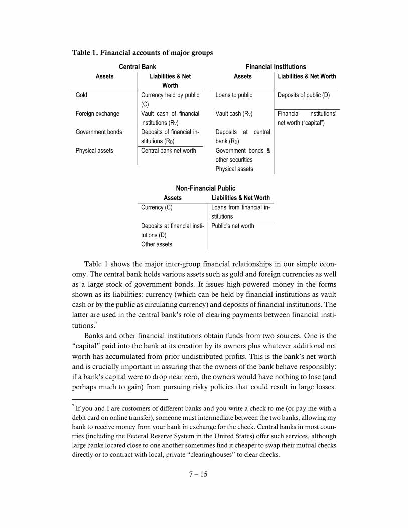
Table 1. Financial accounts of major groups

Central Bank Financial Institutions

Assets Liabilities & Net

Worth

Assets Liabilities & Net Worth

Gold

Currency held by public

(C)

Loans to public Deposits of public (D)

Foreign exchange Vault cash of financial

institutions (RV)

Vault cash (RV) Financial institutions’

net worth (“capital”)

Government bonds Deposits of financial in-

stitutions (RD)

Deposits at central

bank (RD)

Physical assets

Central bank net worth Government bonds &

other securities

Physical assets

Non-Financial Public

Assets Liabilities & Net Worth

Currency (C)

Loans from financial in-

stitutions

Deposits at financial insti-

tutions (D)

Public’s net worth

Other assets

Table 1 shows the major inter-group financial relationships in our simple econ-

omy. The central bank holds various assets such as gold and foreign currencies as well

as a large stock of government bonds. It issues high-powered money in the forms

shown as its liabilities: currency (which can be held by financial institutions as vault

cash or by the public as circulating currency) and deposits of financial institutions. The

latter are used in the central bank’s role of clearing payments between financial insti-

tutions.9

Banks and other financial institutions obtain funds from two sources. One is the

“capital” paid into the bank at its creation by its owners plus whatever additional net

worth has accumulated from prior undistributed profits. This is the bank’s net worth

and is crucially important in assuring that the owners of the bank behave responsibly:

if a bank’s capital were to drop near zero, the owners would have nothing to lose (and

perhaps much to gain) from pursuing risky policies that could result in large losses.

9

If you and I are customers of different banks and you write a check to me (or pay me with a

debit card on online transfer), someone must intermediate between the two banks, allowing my

bank to receive money from your bank in exchange for the check. Central banks in most coun-

tries (including the Federal Reserve System in the United States) offer such services, although

large banks located close to one another sometimes find it cheaper to swap their mutual checks

directly or to contract with local, private “clearinghouses” to clear checks.

7 – 16

Because of this important role in mitigating banks’ incentives to take on excessive risk,

modern financial systems require minimum levels of capital as a percentage of the

bank’s assets.10

The other source of banks’ funds is the deposits of their customers. While capital

is the bank’s net worth, deposits are liabilities that it owes to its depositors.

The major financial assets are the bank’s reserves (held either as vault cash or as

deposits at the central bank), loans to the public, and financial assets such as govern-

ment bonds. Financial institutions have traditionally earned no interest on their re-

serves so they have a profit incentive to hold interest-bearing assets (loans and bonds)

instead.11

However, banks must maintain some reserves both because the central bank

usually requires them to and because they must have sufficient reserves to cover day-

to-day transactions: both withdrawals of cash by customers and transfers out of their

central-bank account that result from the clearing of checks that their customers have

written.

The public holds a variety of assets, but the ones that are important for the financial

system are currency and deposits at banks—money. Their major financial liability is

loans that they have taken out from financial institutions.

Money, the monetary base, and the money multiplier

In the simple economy whose financial accounts are depicted in Table 1, we define

money to include currency and deposits held by the public, M = C + D. The stock of

money includes deposits held at banks, accounts to which the central bank is not a

10

Even with zero or negative capital, banks may continue operations unless forced to close by

regulators or by a flood of deposit redemptions (a bank run). Under modern deposit-insurance

systems, depositors have no incentive to instigate runs, so the burden of closing down insolvent

banks falls to government regulators. If they fail to do so promptly, negative-capital “zombie”

banks have incentives to pursue risky investment strategies in an attempt to get back above

water. (For example, betting 10 percent of bank assets on the Super Bowl might offer a 50/50

chance of making the bank solvent again. Any losses would be borne by the deposit insurer.)

Unscrupulous bank owners and managers may also have incentive to “loot” the bank by en-

gaging in transactions that inflate immediate profits (which can then be withdrawn in bonuses

to executives and dividends to owners) but that incur large losses in the future (when the cost

will be borne by the deposit insurer who has to clean up the debris of the failed bank). See

Akerlof and Romer (1993) for a discussion of looting and Kane (1989) and Curry and Shibut

(2000) for analysis of the impact on taxpayers of not closing down zombie financial institutions

in the 1980s. 11

In the current financial crisis, the Fed began paying interest on banks’ deposits. The interest

rate on reserves is tied to the Fed’s target for the federal funds interest rate, which was lowered

to 0.25% in late 2008 and has begun rising only slowly since 2015. Thus, even under this new

policy the interest available on reserves is small compared with the rate on bank loans.

7 – 17

party. Hence the central bank has only limited ability to “control” the quantity of

money in circulation. It influences the money stock directly or indirectly by manipu-

lating its financial liabilities, which we call the monetary base or the stock of high-pow-

ered money.

The monetary base B consists of the three central-bank liabilities listed in Table 1:

currency held by the public, currency in the vaults of financial institutions, and depos-

its of financial institutions at the central bank. The latter two comprise financial insti-

tutions’ reserves, so we can write the monetary base as B = C + R, where R = RV + RD

consists of vault cash and financial-institution deposits.

The central bank exerts complete control over B. Transaction between other enti-

ties of the economy, such as a decision by a person to deposit currency into a bank

account, can change the composition of B among its components, but cannot influence

the aggregate monetary base. Only when the central bank buys or sells something will

the monetary base change.

In practice, central banks control the monetary base through open-market opera-

tions, buying and selling government bonds to individuals, firms, or financial institu-

tions.12

If the central bank buys a $10,000 Treasury bill, it pays for the open-market

purchase (usually) by crediting the seller’s account (or the seller’s bank’s account) or

(rarely) by giving the seller newly issued currency. These funds always end up in one

or another part of the monetary base, so the open-market purchase increases the mon-

etary base by $10,000 regardless of who sells the Treasury bill to the central bank and

what the seller does with the proceeds.

What remains is to link B, which the central bank controls, to M, which is a varia-

ble through which it affects the economy. We do this by examining the ratio M/B,

which we call the money multiplier. Using the definitions of M and B above,

1,

CM C D D

C RB C RD D

where the final step is achieved by dividing all terms in the numerator and denomina-

tor by D.

Let u = C/D and v = R/D. We can then rewrite the money multiplier as

12

In the recent financial crisis, the Fed expanded its open-market purchases to include a variety

of private assets in addition to government bonds. These transactions served not only to provide

general liquidity to banks by expanding reserves but also to increase liquidity in selected finan-

cial markets that were paralyzed by illiquidity and concerns about counterparty risk.

7 – 18

1.

M u

B u v

(1)

We consider u and v to be behavioral parameters of the economy. The households and

firms in the economy decide on the value of u when they determine how much of their

money to hold as currency vis à vis deposits. For example, if the public holds 90% of

its money as deposits and 10% as currency, then u will be 10%/90% = 0.111. The ratio

v is a decision parameter of financial institutions: the amount of reserves they hold out

of each dollar of deposits. As noted above, financial institutions are usually required

to hold some reserves, so v is bounded from below by official reserve requirements.

However, it is important to note that banks would choose to hold some volume of

reserves voluntarily even if they were not required to do so. In some times and places,

banks have held significant quantities of excess reserves above and beyond reserve re-

quirements.13

The money multiplier therefore depends on two decision parameters, one made by

the public and one by the financial institutions. To the extent that these decisions are

stable and predictable, the central bank can effectively control the money supply by

anticipating what the multiplier will be and manipulating the monetary base to provide

just the desired amount of money. In normal times, u and v do tend to be quite pre-

dictable (and central banks devote a lot of energy to predicting them), so central banks

can usually control M quite effectively.

We call this ratio a “multiplier” because it reflects the degree to which the private

sector “multiplies” the monetary base into a larger stock of monetary assets. If banks

held 100% of their deposits in reserve, then v = 1 and the numerator and denominator

are equal, so the money supply equals the monetary base and the multiplier is one.

However, as we noted in our brief history of money, fractional-reserve banking has for

centuries been the universal norm. If banks hold less than full reserves v < 1 and the

money multiplier exceeds one.

The intuition of multiple expansion of the money supply is easiest to grasp in an

even simpler setting where the public holds no currency (u = 0). In that case, the mul-

tiplier is 1/v. Suppose that an open-market purchase increases the monetary base by

$10,000. Since households hold no currency, this all ends up getting deposited in the

banking system, which increases reserves by $10,000. If banks want to hold a ratio v,

say 0.10, of their deposits in reserves, then this additional $10,000 of reserves will sup-

port 1/v × $10,000 = $100,000 of additional deposits. Thus, the increase in the money

supply is 1/v = 10 times as large as the increase in the base.

13

Excess reserves in the United States exploded after 2008 as the Federal Reserve bought mas-

sive amounts of assets under its “quantitative easing” program. This led to a dramatic decline

in the money multiplier.

7 – 19

It is easy to see both intuitively and in terms of equation (1) that currency holding

by the public (u > 0) will reduce the size of the multiplier. Each dollar that gets held in

currency supports only itself; it does not get deposited into the banking system to be a

dollar of reserves supporting multiple dollars of deposits. The money multiplier de-

pends inversely on both the currency-deposit ratio and the reserve-deposit ratio.

Monetary policy and interest rates

A detailed examination of monetary policy is far beyond the scope of this chapter.

Selected topics of monetary policy are discussed in Romer’s Chapter 12. A detailed

treatment is available in the Reed curriculum in Economics 341: Monetary and Fiscal

Policy.

However, it is very important to attempt to reconcile the monetary control mech-

anism examined above with the contemporary practices of central banks. In their at-

tempts to influence their economies through monetary policy, central banks face a

choice of instruments that they can use. The model we examined above suggests that

central banks would effect their monetary policy by establishing target growth rates for

the money supply, the monetary base, or bank reserves, and central banks have often

used such reserve or monetary-aggregate targets. The West German Bundesbank (be-

fore it became integrated into the European Central Bank after currency union) fa-

mously targeted monetary aggregates. In the United States, the Federal Reserve under

Paul Volcker switched to a strict reserves target in 1979, when inflation was at unprec-

edented levels and public confidence in the dollar was wavering.

Most central banks now use an interest-rate target rather than a monetary target.

If you follow the financial news at all, you undoubtedly hear about the latest Federal

Reserve decision to raise or lower “interest rates.” While interest-rate targeting is con-

ceptually somewhat different than targeting a monetary aggregate, the mechanism

through which monetary policy operates is similar.

The interest rate that the Federal Reserve targets is the federal-funds rate. This is

the interest rate on overnight loans or reserves between banks. Banks that on any par-

ticular day find themselves with reserves in excess of their desired holdings may try to

lend their excess reserves overnight to other banks that are short. 14

The supply of and

demand for federal funds is very sensitive to the reserve position of banks. If reserves

are scarce then there will be more borrowers than lenders and the federal-funds rate

14

Reserve requirements are calculated over a two-week period. The average volume of reserves

over a two-week reserve holding-period must be at least the required fraction of the average

volume of deposits over a corresponding deposit period. The reserve-holding period is lagged

relative to the deposit period so that banks can calculate the average value of their deposits at

the end of the deposit period (and thus know the amount of reserves required) and still have a

few days to make up any deficits in their reserves relative to the requirement.

7 – 20

will tend to rise. If reserves are abundant, then there will be many lenders and the rate

will fall.

Thus, the federal-funds rate acts as a “thermometer” for the scarcity of reserves in

the banking system. When it targets the federal-funds rate, the Federal Reserve in-

creases or decreases the monetary base (and thus bank reserves) in such a way as to

keep the rate—the “temperature” of the reserve market—at the target level. If the Fed’s

target is 3% and the funds rate starts to creep upward to, say, 3.05%, the trading desk

at the Federal Reserve Bank of New York will buy Treasury bills, releasing additional

high-powered money into the economy to act as additional bank reserves. This releases

the upward pressure on the funds rate and pushes it back down toward the 3% target.

Similarly, if the funds rate slips below the target the Fed sells Treasury bills and absorbs

reserves out of the banking system.

In the financial crisis of 2007–08, the federal-funds-rate target essentially reached

zero. Nominal interest rates cannot be negative unless lenders are coerced, so there is

no further possibility of stimulating aggregate demand by lowering this interest rate.

In this case, there are still several stimulative options open to a central bank. It can still

pursue “quantitative easing” by expanding the monetary base rapidly. Although they

cannot drive the federal-funds rate down, they can increase banks’ reserves, which may

encourage them to lend. The central bank can also target its open-market purchases

on particular parts of the credit market that need liquidity or support. For example, the

Fed began purchasing longer-term government bonds, commercial paper, and new

high-quality asset-backed securities in late 2008 to support these markets.

The Fed also began paying interest on banks’ reserve deposits in 2008. This has

caused banks to hold large quantities of excess reserves in place of other interest-earn-

ing assets that were sold to the Fed as part of the latter’s quantitative easing purchases.

If has also changed the nature of the federal-funds market (since banks no longer need

to worry much about meeting reserve requirements) and introduced a new instrument

of monetary policy: the interest rate on these reserve deposits. Since 2008, the reserve

interest rate has been kept aligned with the federal-funds-rate target.15

15

The monetary aspects of the 2008 financial crisis are discussed in more detail in Section H of

this chapter.

7 – 21

F. Theories of the Demand for Money

Quantity theory: Money in the classical macro model

Money is a stock. At every moment there is a stock quantity of monetary assets

available to satisfy the needs of consumers and firms. In contrast, the principal use of

money—spending—is a flow. Thus, theories of the demand for money have a tem-

poral dimensionality that relates the stock of dollars held to the flow of dollars spent

per year. In the quantity theory of money, our simplest theory of money demand, that

temporal dimensionality takes the form of the velocity of money: how many times per

year the average dollar is spent.

The quantity theory is how the classical economists completed their general-equi-

librium system by explaining the role of money and the determination of the level of

prices.16

Classical economists took a narrow view of the role of money in the economy.

They believed that money was held as an asset solely for its liquidity—its ability to be

used in transactions—so the quantity of money demanded would be locked tightly to

the volume of transactions individuals undertook. The connection between the stock

of money held and the flow of transactions is called the transactions velocity of money,

defined as

,T

PQV

M (2)

where PQ is the total nominal quantity of transactions in the economy and M is the

stock of money. Because it is the ratio of a flow to a stock, transactions velocity has

the temporal dimension of “number per period.” Since we are assuming that all trans-

actions are made with money, transactions velocity measures how many times per

year the average dollar is spent. For example, if there are $500 billion dollars in the

economy and total transactions are worth $10 trillion, then transactions velocity would

be $10 trillion/$500 billion = 20 times per period.

Because it is difficult to measure the total value of all transactions (including those

for intermediate goods) in the economy, we usually work with income velocity, which

is the number of times per year the average dollar is spent on final goods and services.

Income velocity V can be computed as

16

Although there were several variants of the quantity theory, they led to largely similar conclusions.

A typical classical exposition can be found in Irving Fisher (1913). A more modern version is Milton

Friedman’s famous article “The Quantity Theory of Money: A Restatement,” which is reprinted as

Chapter 2 of Friedman (1969).

7 – 22

,PY

VM

(3)

where Y is real GDP and thus PY is nominal GDP, equal to the GDP deflator P times

real GDP.

The classical quantity theory stems from assumptions about the behavior of the

variables in equation (3).

First, microeconomic factors such as those in the real-business-cycle model are

assumed to determine real GDP in a way that is independent of monetary fac-

tors.17

Second, the income velocity of money was thought to depend on such charac-

teristics of the monetary system as whether people used cash or checks and the

general desire of people to hold money.

Finally, the supply of money was viewed as exogenously determined by the

central bank, backed in classical times by its reserves of gold under the gold

standard.

With Y and V determined by nonmonetary factors, equation (3) implies a lock-step

connection between exogenous changes in the money supply and the general price

level,

.V

P MY

(4)

Equation (4) shows that changes in the money supply lead to exactly proportional

changes in the general price level (and in all nominal prices in the economy, including

wages and foreign-exchange rates), but to no changes in real variables. This classical

result is known as monetary neutrality. It holds in the quantity-theory framework as

long as V and Y are not influenced by changes in the money supply.

Quantity theorists varied in the rigidity with which they held these assumptions.

The so-called “Cambridge school” of English classical economists recognized that

changes in interest rates could affect the desire to hold money vis-à-vis other assets and

17

The classical dichotomy refers to the segregation of the economy into two separable parts: the real

side and the monetary sector. Under classical postulates, the real side of the economy is assumed to

be completely independent of any monetary factors. All of our growth and RBC models, because

they have assumed that the real side of the economy could be determined without reference to

money or prices, have followed the classical dichotomy.

7 – 23

therefore could affect velocity.18

Higher interest rates make interest-bearing assets more

attractive relative to money and may therefore reduce desired money holding and in-

crease velocity. If monetary changes cause interest rates to change, velocity might be

affected and the relationship between money and prices would not be strictly propor-

tional.

Irving Fisher and other American theorists were more faithful to the assumption

that monetary changes would not affect velocity and pushed a stricter version of the

quantity theory. Fisher was also convinced that changes in the money supply could

not affect interest rates in a sustained or substantial way.

More recent quantity theorists such as the late Milton Friedman adopted a much

more flexible approach to equation (4). Friedman recognized that money might affect

interest rates—and therefore velocity and even real output—in the short run. But he

argued that interest rates, velocity, and real output should be independent of monetary

influences in the long run, so that equation (4) would still hold over longer periods of

time. Many important models of modern macroeconomics lead to this same general

conclusion: money is neutral in the long run but has real effects in the short run.

The evolution of money-demand theory

The demand function for money is one of three major behavioral relationships of

early Keynesian macroeconomic models. (The other two are the consumption and in-

vestment functions.) The “standard” formulation of money demand makes the real

money holdings a function of real income and the nominal interest rate. This formula

fit the data very well for the first three decades after World War II, leading macroe-

conomists to place considerable confidence in the stability of the money-demand rela-

tionship.

However, like other empirical macroeconomic relationships, the performance of

the money-demand function deteriorated rapidly with the arrival of ongoing inflation

in the 1970s. The first indication that something was amiss was documented in a study

by Stephen Goldfeld creatively called “The Case of the Missing Money.” Goldfeld

(1976) noted that empirical money demand functions started veering off course in the

1970s, predicting that people should have been holding much larger real money bal-

ances than they actually were, hence the “missing money” in his title. In terms of the

quantity theory, the velocity of money was unexpectedly high in the 1970s relative to

the prediction of the earlier model.

As usually happens with empirical conundrums, the case of the missing money

spawned a large empirical literature seeking to explain the decline in money holdings.

18

The Cambridge school cast its theory in terms of the reciprocal of velocity, the Cambridge k, which

is the ratio of money holdings to nominal income.

7 – 24

Some argued that the rise of credit-card use was an important factor; others stressed

that high inflation caused firms and financial intermediaries to devise new methods to

economize on non-interest-bearing deposits. The introduction of new kinds of finan-

cial assets—money-market mutual funds, certificates of deposit, and money-market

deposit accounts, to name three—changed the definition of the money supply and

complicated the already-difficult task of finding a stable empirical relationship.

Since the 1970s, money demand has behaved erratically. Predictions from esti-

mated models have sometimes missed on the high side and sometimes missed on the

low side. Many macroeconomists have lost confidence in the ability to predict the re-

lationship between money demand and its presumed determinants, interest rates and

income. This has been a particular problem for policymakers at the Federal Reserve,

who rely on the money-demand function as a crucial lever in the connection between

their monetary-policy instruments and the real economy.

The empirical instability of money demand mirrors the unsatisfactory state of our

theoretical understanding of the demand for money. As noted above, the Walrasian

general-equilibrium model includes no role for money. We need money in the real-life

economy because of uncertainty and transaction costs, which the standard microeco-

nomic setup ignores. Economists have made only limited progress in modeling these

imperfections, so money-demand theory is often based on a somewhat shaky frame-

work.

Keynes’s three motives for money demand

In the General Theory, Keynes identified three motives for holding money. Individ-

uals have a transactions motive to hold money for use in transactions that they plan to

undertake. This category of money demand is consistent with the thinking of the quan-

tity theory.

The precautionary motive causes people to hold extra money to deal with uncer-

tainty about the flow of expenditures. Since you never know when you will need

money for cab fare on a rainy night or when you will encounter an unexpected bargain,

it is always useful to have a little extra money available for unexpected purchases.

Finally, under certain special conditions an individual might expect to earn a higher

rate of return on money than on other assets, which would result in a speculative motive

for holding some monetary assets.

Keynes argued that the transactions and precautionary demand for money would

depend largely on the volume of transactions undertaken in the economy, while the

speculative demand would depend on the interest rate. Thus, Keynes ended up with a

money-demand function that featured the two variables that have been central to

money-demand theory ever since: aggregate income and the interest rate. Modern the-

ories have shown that transactions and precautionary demand should also depend on

7 – 25

interest rates, which has reduced the importance of speculative demand in providing

an explanation for the interest elasticity of money demand.

In the following sections, we will consider simple models of each of these motives

for holding money. What complicates the analysis is that money balances held for one

purpose may be available for other purposes as well, so one cannot just add up demand

arising from the three motives separately to get a total demand. Since the models are

difficult to combine in a single integrated framework, standard textbook treatments of

money demand usually present one or more models each of which is focused on a

single motivation for holding money. They then assert that one can (magically) com-

bine these models to yield a general demand function.

The money-demand decision

To someone who has not studied economics, it may seem silly to be talking about

the “demand for money.” Doesn’t everyone always want more money? Of course the

answer is yes if there is no opportunity cost to holding money. However, in thinking

about the demand for money, it is crucially important not to confuse “money” with

“wealth.” Individuals always want more wealth, other factors held constant, but they

may not always want to hold more money. The demand for money is not a decision

about how much wealth an individual would like to command (where more is always

better). It is a decision about how much of one’s given stock of wealth should be held

in the form of money rather than as other assets such as bonds.

Thus, when we model the demand for money, we put agents in a situation where

they have a fixed stock of wealth that they must allocate among two or more assets,

one of which is money. The simplest (and most common) modeling framework has

two assets, money and bonds. These assets differ in two basic ways.

First, money is liquid in that it can be used in making transactions in the

goods market; bonds cannot.

Second, money is assumed to bear a zero nominal interest rate while bonds

bear interest at nominal rate i.

Thus, holding money yields liquidity services to the agent, but incurs a forgone-interest

cost. Optimal money holding balances the marginal (liquidity) benefit of money hold-

ing with the marginal (interest) cost.

Baumol and Tobin’s transactions-demand model

Perhaps the most famous treatment of transactions demand is the inventory-theo-

retic model developed by William Baumol (1952) and (independently) James Tobin

(1956). In this model, households receive their income in lump sums at the beginning

of each period, but make expenditures smoothly through time. They hold inventories

7 – 26

of money to enable the flow of expenditures and the flow of income to be asynchro-

nous.19

The motivation for holding money in this model is that money must be used in all

goods-market transactions. However, as noted above, there is an opportunity cost of

holding money: the interest forgone on an interest-bearing asset such as a bond. In

order to maximize interest earnings, the agent would like to hold as much of her wealth

as possible in the form of bonds, while still being able to finance her flow of monetary

expenditures.

If there is no cost to transferring wealth between bonds and money, she could keep

all of her wealth in the form of the “bond” and transfer an appropriate amount into

money an instant before she wanted to spend it, allowing her to earn interest on the

bond until the last moment. This money-holding strategy would drive average money

holdings to zero, since positive money holdings would only occur for a vanishingly

short instant. However, if her flow of expenditures were smooth through the period,

she would need to make many transfers from bonds to money in order to implement

this strategy. Making these transfers generally incurs some kind of cost, either explic-

itly through a transaction fee or implicitly through the time and inconvenience of mak-

ing the transfer. This cost may easily outweigh the interest that is earned from a few

hours or minutes of additional bond-holding.20

The Baumol-Tobin model derives the optimal frequency of bond-money transfers

that minimizes the sum of the two components of cost: the forgone interest cost (which

rises as average money balances increase) and the bond-to-money transaction cost

(which falls as fewer money-bond transfers are made and more money is held). The

strategy that minimizes total cost makes real money demand equal to

,2

M YF

P i (5)

where Y is real income, F is the real cost of making a transfer from bonds to money,

and i is the nominal interest rate. Note that equation (5) expresses the demand for

money in real terms. Changes in the price level P increase the nominal demand for

money exactly in proportion, leaving the real amount demanded unchanged.

19

One can derive a similar result from a model in which expenditures are lumpy and income arrives

smoothly. The key features of the model are that income and expenditures are not synchronized and

that at least one flow is fairly smooth. Any model having these features will lead to a demand for

money result that is similar to the one in the Baumol-Tobin model.

20

Moreover, interest-bearing accounts at financial institutions, which are the most liquid inter-

est-bearing assets, only calculate interest daily, so one could not gain any additional interest by

making more than one bond-to-money transfer per day.

7 – 27

Equation (5) shows that increases in real income lead to greater money demand;

more transactions require additional money holdings. A higher cost of money/bond

transactions also raises money demand, since it becomes more costly to replenish

money balances frequently. A higher interest rate lowers money demand because more

bond interest is forgone for each dollar held as money.

It is interesting to consider what happens to equation (5) in various limiting cases.

As i goes to zero, the demand for money becomes infinite, which means that agents

want to hold all of their wealth in the form of money rather than interest-bearing assets.

This makes sense because as the nominal interest rate approaches zero, the interest

benefit of holding bonds vanishes. Since money still provides superior liquidity ser-

vices, there is no reason to hold bonds. We shall encounter this situation in later chap-

ters; Keynes called it a liquidity trap.

A second interesting limiting case occurs when the transaction cost F approaches

zero. If there is no transaction cost, we are in the ideal world we considered earlier,

where an individual can costlessly transfer bonds to money an instant before making

each transaction and the demand for money would approach zero. While we do not

yet live in this perfect world, modern innovations in banking technology have made

such transactions much less costly in time and inconvenience. This has probably low-

ered the demand for non-interest-bearing money as more households find it beneficial

to keep wealth in an interest-bearing form for a larger portion of the pay period.

While the Baumol-Tobin approach to money demand yields insights on certain

aspects of money-holding behavior, it is subject to important criticisms. First, it takes

the timing of income receipts and expenditures to be exogenous. As a society, these

institutional factors can and do vary in response to economic conditions and incen-

tives. For example, during the German hyperinflation of the 1920s, workers were re-

portedly paid twice daily so they could spend their morning earnings during the lunch

hour, before inflation depreciated their value in the afternoon. Closer synchronization

of income and expenditures reduced the demand for money without agents having to

make more money-bond transfers. As another example, many kinds of expenditures

in modern economies occur in a lumpy pattern. We pay rent, utility bills, car pay-

ments, and credit-card bills once per month. If we can synchronize the due dates of

these bills with our pay date(s), we can substantially reduce the average amount of

money we need to hold in our checking accounts.

A second criticism relates to the empirical evidence on the money demand func-

tion. The Baumol-Tobin model asserts that the elasticity of real money balances with

respect to income should be ½ and that the elasticity with respect to the interest rate

should be –½. As discussed in Case Study 18–3 in Mankiw (2010), the empirical evi-

dence suggests that the interest elasticity is smaller and the income elasticity larger

than these predicted values. Evidence also suggests that elasticities are greater in the

long run than in the short run (contrary to the theory).

7 – 28

Finally, the tradeoff analyzed in the Baumol-Tobin model is one that is relevant

for only a small subset of the population. Suppose that the interest rate is 6% per year,

or ½% per month. A person who earns and spends $48,000 per year (or $4,000 per

month) holds $2,000 in average money balances if she buys no bonds and holds all

unspent income in the form of money ($4,000 on payday, decreasing to zero just before

the next paycheck). By making one extra bond-money transfer, she can reduce average

money holdings to $1,000 and hold an average of $1,000 in bonds. The interest earned

on this $1,000 of average bond holdings is $1,000 0.005 = $5.00. When all explicit

and implicit costs of making the transfer are taken into account, it seems unlikely that

very many people would find this worthwhile. It is even less likely if, as is usually the

case, a substantial fraction of monthly income is paid in a lumpy manner through bills

or large shopping trips. Suppose that $2,000 per month is spent immediately on rent,

utilities, and other beginning-of-month expenses. Then the amount of smooth monthly

expenditures is only $2,000 (half as much as before) and the interest earned by making

the extra transfer is only $2.50.

Modeling precautionary demand

Our model of the precautionary demand is based on the exposition of David

Laidler (1993). It uses a simple representation of the stochastic, or random, behavior

of expenditures. The stochastic approach departs from the Baumol-Tobin model, in

which the agent knows the amount and timing of both income and expenditures with

certainty. Under certainty, she is able to replenish her money holdings at the exact

time they are exhausted. A more realistic model of expenditures should include unpre-

dictable variability in the flow of expenditures (and perhaps in income as well).

In our model, the agent will undertake an amount of expenditures that varies from

expected spending by a random variable S that has mean zero and standard deviation

S. If the agent holds enough extra money (beyond the amount used for expected trans-

actions) to cover whatever unexpected expenditures occur, then she is able to make

the expenditures without incurring any additional cost. However, if her precautionary

money holdings are insufficient to cover expenditures, she incurs a “brokerage cost”

(which might include time, inconvenience, and other implicit components) equal to b.

The agent’s objective in deciding how much “precautionary money balances” to hold

is to minimize the sum of two components of cost: the expected brokerage cost and

the forgone interest cost. Both are a function of the amount of precautionary money

held: an increase in money balances lowers the expected brokerage cost because the

agent is less likely to run short, but increases the forgone interest cost.

Suppose that the volume of unexpected expenditures S follows a probability distri-

bution with density function f (S), so that the probability that S is less than or equal to

some specific value s is

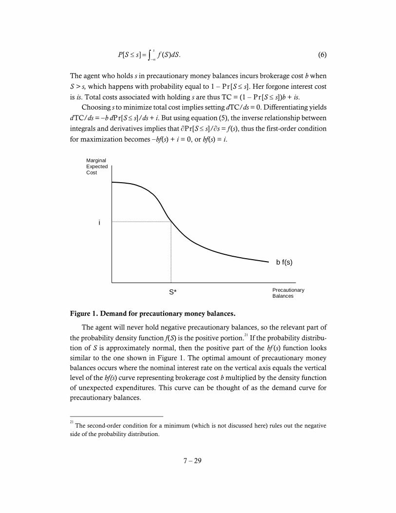
7 – 29

[ ] ( ) .s

P S s f S dS

(6)

The agent who holds s in precautionary money balances incurs brokerage cost b when

S > s, which happens with probability equal to 1 Pr[S s]. Her forgone interest cost

is is. Total costs associated with holding s are thus TC = (1 Pr[S s])b + is.

Choosing s to minimize total cost implies setting dTC/ds = 0. Differentiating yields

dTC/ds = b dPr[S s]/ds + i. But using equation (5), the inverse relationship between

integrals and derivatives implies that Pr[S s]/s = f (s), thus the first-order condition

for maximization becomes bf(s) + i = 0, or bf(s) = i.

Marginal

Expected

Cost

Precautionary Balances

b f(s)

i

S*

Figure 1. Demand for precautionary money balances.

The agent will never hold negative precautionary balances, so the relevant part of

the probability density function f(S) is the positive portion.21

If the probability distribu-

tion of S is approximately normal, then the positive part of the bf (s) function looks

similar to the one shown in Figure 1. The optimal amount of precautionary money

balances occurs where the nominal interest rate on the vertical axis equals the vertical

level of the bf(s) curve representing brokerage cost b multiplied by the density function

of unexpected expenditures. This curve can be thought of as the demand curve for

precautionary balances.

21

The second-order condition for a minimum (which is not discussed here) rules out the negative

side of the probability distribution.

7 – 30

It is easy to examine the effects of exogenous changes on precautionary balances

using Figure 1. An increase in the nominal interest rate raises the opportunity cost of

holding precautionary balances and reduces optimal holdings along the demand curve.

If brokerage cost increases, that raises the cost of being caught short and shifts the

demand curve outward, leading to higher precautionary balances at any given interest

rate. Finally, if expenditure patterns become less predictable due to an increase in S,

the standard deviation of unexpected expenditures, then the probability density func-

tion f (s) will spread toward the right, shifting the demand curve outward and leading

to higher precautionary balances.

How does this theory relate to contemporary trends in the banking industry? It is

likely that new technologies in banking have affected both b and S in ways that have

lowered the precautionary demand for money. The wide availability of automatic

teller machines and increasing acceptability of credit cards have likely made the bro-

kerage cost of being caught short of M1 (especially currency) much lower than it was

before. This lowers b and shifts the demand curve down proportionally. This effect has

likely lowered the precautionary demand for the currency component of M1 greatly.

You still need money in the bank to use your ATM card, so the effect on the demand

for total M1 and on M2 are probably smaller than the effect on currency demand.

Since most unexpected expenditures can be “smoothed out” by using a credit card

for the original transaction, variation in actual payments has probably fallen in recent

decades. This too would lower the demand for precautionary balances by shifting the

demand curve to the left.

Is there a speculative demand for money?

The conventional interpretation of the speculative demand for money in the post-

war Keynesian literature was the model developed by James Tobin (1958) in his fa-

mous paper “Liquidity Preference as Behavior Towards Risk.” This model looked at

the optimal allocation of a wealth-holder’s portfolio between a risky interest-bearing

asset and a safe asset—money. Tobin showed that risk-averse wealth-holders would

hold some positive amount of money in order to reduce the risk of their overall port-

folios.

This approach has a couple of major flaws as an explanation for the speculative

demand for money in modern economies. First, money is not necessarily a safe asset.

If inflation is subject to uncertainty then although the nominal rate of return on money

is known to be zero, the real return (which is the nominal return minus the inflation

rate) will vary unpredictably. Second, there are assets such as short-term Treasury bills

that pay positive nominal interest and that also have negligible nominal risk. Tobin’s

model may explain the demand for these assets as agents attempt to reduce risk in their

portfolios, but it is unclear why an agent would use currency or demand deposits for

this purpose.

7 – 31

Despite the problems with Tobin’s formulation, it is possible to develop another

motivation for speculative balances based on Keynes’s original argument. Keynes mo-

tivated the speculative demand for money by considering the behavior of someone

who believes market interest rates are likely to rise in the near future. Such an individ-

ual will expect that the secondary-market price of existing bonds will fall when interest

rates rise, so that he expects to suffer a capital loss if he holds bonds.22

If the average investor in the market believes that the interest rate is likely to rise,

then there will be a general sell-off of bonds, which will raise interest rates immediately

and extinguish the expectation of an increase and with it the average agent’s specula-

tive demand for money. Thus, the average market participant cannot have a positive

speculative demand for money for more than an instant. However, if expectations vary

across participants in the market, then those few individuals with expectations about the

immediate course of interest rates that are much higher than average could find that

they would earn a higher expected rate of return by holding money than by holding

bonds. Thus, the fringe of market participants with the most extremely “bearish” view

of future prices of bonds (or other non-money assets) might hold extra money balances

above and beyond those necessary for transaction and/or precautionary purposes.

Some of the criticisms of the transactions-demand model apply here as well. Some

bank deposits (such as savings accounts and money-market accounts) have interest

rates that vary with market rates. Money deposited in these accounts would not suffer

a capital loss, but would instead immediately start earning the higher rate of interest

after the market rate increased. Since there would be no capital loss on these assets, an

agent who wanted to avoid a capital loss would be better off putting his money in one

of these than in currency or demand deposits. Thus, this argument for the speculative

motive for money holding might apply to the broader definitions of money that in-

cludes such assets (M2 and M3) but would not be appropriate for M1.

22

Recall that the market price of existing bonds is inversely related to the market interest rate on

new bonds. The following example may clarify this relationship. Suppose that an individual pur-

chases a brand-new $1,000 bond with an interest rate of 5% with principal and interest due in one

year. This person will get a payment of $1,050 in one year. Now suppose that later in the day the

market interest rate on one-year bonds goes up to 10%. New bonds priced at $1,000 will now yield

$1,100 in one year, so the old bond that promises to pay $1,050 cannot be worth $1,000 after the

change in the interest rate. The present value of the $1,050 payment when the market interest rate

is 10% is $1,050/(1.10) = $954.55. Thus, the agent has incurred a capital loss of $45.45 due to the

increase in the market interest rate on new bonds. The capital loss is larger the longer the term of

the bond. In the case of a perpetuity that never matures, the loss would be $500 or half of the original

investment! Clearly the negligible amount of interest earned in a few hours (which we have ignored

here) is minuscule compared with the capital loss.

7 – 32

An integrated model of money demand

In his text on monetary economics, Bennett McCallum (1989) develops a model

in which the demand for money is integrated with the general utility-maximization

problem of the household.23

McCallum chooses to put money in the household’s

budget constraint. The household’s time is now assumed to be devoted to three activ-

ities: work, leisure, and making transactions. Holding larger money balances (for a

given flow of consumption expenditures) saves the household transaction time, allow-

ing leisure (or work) time to be higher, which gives greater utility. This is an example

of a so-called “shopping-time” model.

Formally, the households maximize discounted lifetime utility. Utility in each pe-

riod is a function of consumption and leisure in the period. Thus, households maxim-

ize

0

1( , ).

(1 )t tt

t

U u c l

(7)

The household’s work decision is assumed to be already made independently of the

money-holding and consumption decisions, so the household earns yt in period t and

devotes a fixed amount of time to work.

Households maximize (7) subject to two constraints. The first is the budget con-

straint that the present value of the lifetime stream of consumption equals the present

value of the lifetime stream of income. This budget constraint must be slightly altered

to recognize that the part of the household’s financial wealth that is held in the form

of money does not bear interest. The basic building block of the lifetime budget con-

straint is the intertemporal condition

1 1 1,t t t t t t t t tP c B M P y i B M (8)

where Bt is net bond holdings (net lending) at the end of period t and Mt is net money

holdings at the end of t, both expressed in nominal terms, ct and yt are real consumption

and income in t, and it 1 is the nominal interest rate on bonds (lending) held from

period t 1 to period t. The left-hand side of equation (8) measures nominal uses of

funds in period t; the right-hand side is nominal sources.

If the nominal interest rate is constant at some value i, the inflation rate is constant

at , the initial price level P1 is normalized to one, and initial and terminal holdings of

bonds are both assumed to be zero, then solving for Bt and substituting repeatedly

yields

23

See his Chapter 3.

7 – 33

1

1 1 1

,(1 ) (1 ) (1 )

t t t t

t t tt t t

c M M y

r i r

(9)

where r i . Note that the real variables c and y in equation (9) are discounted at

the real interest rate, while the nominal variable M is discounted at the nominal interest

rate. This property has important implications. The opportunity cost of current con-

sumption is (1 + r) units of future consumption while the opportunity cost of one dollar

of current money holding is (1 + i) dollars of future money holdings. This implies that

the demand for consumption goods will depend on the real interest rate r while the

demand for money depends on the nominal rate i.

The second constraint applying to the consumer is that leisure in each period de-

pends on the amount of consumption the household does (number of transactions) and

the amount of real money it holds, so lt = (ct, mt). The partial derivatives of the

function are /ct < 0 and /mt > 0. More consumption expenditure with the same

amount of money means that more time must be devoted to transactions and less is

available for leisure. Holding higher money balances for any given amount of con-

sumption means transactions require less time and more leisure is available.

McCallum shows that the solution of this consumer-maximization problem yields

a highly conventional demand function for real money balances that depends nega-

tively on the nominal interest rate and on positively the real volume of consumption

expenditures. Thus, it is possible to embed the money-demand problem in a general

model of consumer equilibrium and derive a result that is consistent with the other

models we have studied: Higher transaction volume means more money demand,

while higher nominal interest rates mean lower demand.

New Keynesian LM curve

In Romer’s Chapter 6, he develops a model of money demand and uses it to con-

struct a new Keynesian LM curve. We will discuss this model in more detail in course-

book Chapter 9, but a brief glimpse is provided here for comparison with the other

theories of money demand.

Consumers are assumed to have a utility function as given by Romer’s equation

(6.2), with CRRA specifications (6.3) and (6.4). Unlike McCallum’s model, in which

holding money saves time and allows more leisure, real money balances are assumed

here to yield utility directly. This is simple, but not very realistic. Money balances do

not typically make people happy, but it is an easier way to give people a reason to hold

them so this formulation is common.

Since the utility function is additively separable in consumption, money, and la-

bor, we can ignore the other terms and focus solely on utility from money holding:

1

0

/.

1

t tt

M

t

M PU

7 – 34

The budget constraint is Romer’s equation (6.5), which describes the accumulation of

nominal assets:

1 1 ,t t t t t t t t tA M A W L PC M i

where it is the nominal interest rate.

Maximizing utility subject to this constraint yields the money-demand equation

1/

/ 1.t t

t

t t

M iY

P i

Thus, real money demand depends positively on real income and negatively on the

nominal interest rate, as in the conventional formulation.

G. Money in Economic Growth Models

Simple macroeconomics of money and growth

The simple models of money demand described above suggest that the real de-

mand for money should depend on the volume of real transactions, often proxied by

real GDP, the opportunity cost of holding money, usually measured by a short-term

nominal interest rate, and transaction costs, which are usually left out for lack of a

convenient measure. This simple model of money demand can be written

, ,

d

eML Y r

P

(10)

where r + e is the nominal interest rate: the sum of the real rate and the expected rate

of inflation.

Despite the prediction of the Baumol-Tobin model that the elasticity of money

demand with respect to income should be one-half, empirical evidence supports the

conclusion that it is close to one. If the income elasticity is one, then we can rewrite

equation (10) as

eM

Y L rP

. (11)

We now consider the relationship between money, inflation, and economic

growth in a long-run steady-state equilibrium. If we take the growth rate of both sides

of equation (11), we get

7 – 35

1

.

e

e

dL iM P Y

M P Y dt L i

In steady-state equilibrium, the interest rate and the (expected) inflation rate will be

constant, so the last term vanishes. Thus, if the growth rate of money is , the rate of

price inflation is , and the growth rate of real output is g, then

.g (12)

Equation (12) is the fundamental steady-state inflation equation that follows from the

standard demand-for-money equation. Most basic formulations of monetary growth

models lead to a conclusion that is similar to (12).

Building money into the microfoundations of growth models

With the exception of the McCallum model and Romer’s LM model discussed at

the end of Section F, all of the money-demand models discussed above have the weak-

ness that they are ad-hoc formulations that are not integrated in any way with the usual

utility-maximization framework of the general-equilibrium microeconomy. Modern

theorists usually integrate money into household-level macro models by one of several

simple mechanisms. Among the simplest (and most common) is imposing a cash-in-

advance constraint. In a discrete-time model, a cash-in-advance constraint forces house-

holds to hold an amount of money at the beginning of each period that is at least as

great as its expenditures for that period. This is essentially a return to the quantity

theory, because it ignores the possibility of varying money holdings by making more

money-bond transactions in order to earn additional interest.

More sophisticated models try to give money a role in household’s utility maximi-

zation or in firms’ production process. The simplest way to do this is to add real money

balances to the utility function or production function. For households, this is prob-

lematic because we do not usually think of money as yielding utility directly—it is a

means to an end rather than an end in itself. Similarly, incorporating money as a factor

of production fails to examine how money is used by firms to reduce costs or increase

output.

A formal analysis of these models is beyond our scope here, but a detailed treat-

ment can be found in the early chapters of Walsh (2003).

7 – 36

H. The Financial Crisis of 2008–09

Most of you do not have extensive training in financial markets, so we’ll begin

with a brief introduction to some of the main components of the crisis. From there we

will proceed to an analysis of how they have combined together to cause the Great

Recession. Finally, we will discuss the policies that the Bush and Obama Administra-

tions pursued in trying to right the economy.

Major elements of the crisis

Housing bubble. U.S. urban residential real estate had been increasing in value

rapidly since the 1980s. In some places, the increase was meteoric. Once peo-

ple begin to expect home prices to rise, they build such expectations into their

financial plan. They begin to speculate on houses or to buy homes that they

cannot really afford with the confidence that they will be able to sell them at a

profit if they cannot make their payments. Similarly, financial institutions are

willing to lend on very generous terms (including low down payments and

minimal credit checking) because they anticipate that the collateral asset

pledged to them in case of default will appreciate. When expectations of rising

prices fuel the demand that increases prices even more, a bubble occurs. All

bubbles eventually burst and the U.S. housing bubble seems to have peaked in

2007. Since then, prices have fallen in most urban markets and have fallen the

most in those markets where they rose the most. When home prices fall, the

value of some properties will fall near or below the amount owed on the mort-

gages. If the owner needs to sell, the proceeds from the sale will not cover re-

payment of the mortgage, so the owner would take a loss. This gives “under-

water” owners a strong incentive to default on their mortgages, leaving the

lender with the devalued collateral and transferring the loss to the lender.

Sub-prime mortgage loans. Traditional or “prime” mortgage loans must ad-

here to some basic safety guidelines. In order to qualify for guarantees by the

quasi-federal institutions Fannie Mae and Freddy Mac, the loan must be less

than 80 percent of the appraised value of the home and the borrower must have

sufficient income and credit background to assure the likelihood of repayment.

Sub-prime loans are ones that do not satisfy these standards. They are riskier

because the cushion of collateral value over the loan value is smaller (less than

20 percent) and/or because the borrower’s creditworthiness has not been sat-

isfactorily established. Sub-prime loans present little problem in an environ-

7 – 37

ment of rapidly rising home values. Even a loan for 100 percent of the ap-

praised value will be down to 80 percent within a couple of years if property

values are spiraling upward at 10 percent per year, as occurred in many prop-

erty markets in the early 2000s. The dodgiest of the sub-prime loans also low-

ered borrowers’ payments for the first few years, adding to the outstanding

loan balance over time but reducing the probability of early default. Availabil-

ity of these loans expanded the demand for houses and fueled the bubble in

house prices. The inevitability of collapse is obvious once prices stopped rising

rapidly.

Securitization. In the old days, banks and “thrifts” (savings and loan associa-

tions and their kin) simply lent depositors’ money. A customer took out a mort-

gage to buy a house and that mortgage remained on the bank or thrift’s books

as an asset until it was gradually repaid over a period of 15 to 30 years. Holding

long-term, illiquid assets such as mortgages can be risky for banks because the

liability side of their balance sheets is dominated by short-term deposits.

Should they suffer a sudden, large withdrawal of deposits, the bank would not

be able to “call in” these mortgage loans. To avoid this liquidity risk, banks

began during the 1990s to “securitize” mortgages and other loans on a large

scale. A pool of similar mortgages was bundled together into a set of mortgage-

backed securities (MBSs) and sold to other investors such as pension funds.

Each MBS was a claim on a part of the payments stream of the bundle of mort-

gages. The bank continued to process the borrowers’ payments and then

passed them along to the holders of the corresponding MBSs. Securitization

was beneficial to banks because it allowed them to do what they do best—

dealing with retail customers, evaluating their credit risks, and processing their

payments—without having to hold very-long-term mortgage assets on their

books.24

However, as Quigley (2008) points out, when banks plan to extinguish

their creditor position quickly by selling off their loans, they may have weak-

ened incentives to evaluate credit risk adequately and to disclose adverse credit

information to prospective buyers of MBSs.

Collateralized debt obligations. Mortgage-backed securities allow the banks

to offload their long-term lending commitments to others who desire to hold

such assets. However, there may be investors who want long-term assets such

as mortgages but who have a greater or lesser tolerance for risk than the overall

MBS would offer. Modern financial institutions have become expert at tailor-

ing exotic derivative securities to transform and calibrate the risk, maturity, and

24

For brief discussion of securitization in the recent past, see Rosen (2007).

7 – 38

return of existing securities. Collateralized debt obligations (CDOs) take an asset

such as an MBS and slice it up into prioritized “tranches” with differing levels

of risk. The highest tranche gets first claim on the stream of payments made by

the bundle of mortgage borrowers, making it relatively safe. Mid-level (“mez-

zanine”) tranches are paid next, assuming that defaults are few enough to keep

the payments stream adequate. The bottom tranches are analogous to a water

user at the very end of the river: if enough payments come through (because

there are no defaults) they will get the full amount of income, but if defaults

are high there may be nothing left once the upstream tranches have taken their

cuts.

Credit-default swaps. Another exotic derivative that emerged in the last dec-

ade is the credit-default swap (CDS). These assets are essentially insurance pol-

icies that banks can take out to protect themselves from loan defaults. While

this might seem like a terrific idea to reduce a bank’s default risk—and it is for

an individual bank—an insurance policy is only valuable if the insurer is finan-

cially healthy. In a general financial crisis, uncertainties about the creditwor-

thiness of CDS counterparties (insurers) may raise doubts about the solvency

of banks. Mengle (2007) provides an introduction to CDSs.

Downturn

All bubbles eventually burst. U.S. urban housing prices peaked in about September

2006 and began to decline. As noted above, the most speculative sub-prime mortgages

were a time bomb waiting to explode as soon as the inflation in property values began

to ebb. The banks that had pushed these loans most aggressively naturally began to

lose money and their cushion of capital was squeezed.

Foreclosing homes is very costly for lenders. By some estimates, banks lose an

average of 40 percent on loans that have to be foreclosed. It is often in the mutual

interest of lender and borrower to “work out” a new loan that stretches out payments

and perhaps lowers interest rates a little bit. In most property crises this has been com-

mon practice and a large fraction of non-performing loans have been renegotiated to

avoid foreclosure.

However, any workout loan must be agreed upon by both the borrower and the

lender. This is easy when the bank itself is the sole lender but can be impossible when

hundreds of owners of mortgage-backed securities and collateralized debt obligations

each hold tiny stakes on the lending side. Short of a “cram-down” provision by a bank-

ruptcy court (which they cannot at present do on mortgages, though permissive legis-

lation has been considered), there is no practical way to get all the fractional lenders

to agree to a workout loan.

7 – 39

This is not the only way in which repeated division and resale of mortgages

through MBSs and CDOs caused difficulties when the housing market turned down.

The opaqueness of these securities caused transaction partners of large financial insti-

tutions to worry about whether they would be able to fulfill their obligations.

This “counterparty risk” has traditionally been a worry in check-clearing and sim-

ilar interbank transactions, as well as in transactions on major stock, bond, and com-

modity exchanges. In these situations, the exchange or clearinghouse usually “nets”

out the vast volume of transactions of each participant, cancelling debits with credits

so that only the net amount must be settled at the end of the day. But many modern

derivative securities, including MBSs and CDOs, are not traded on an exchange. This

means that transactions are not netted, which greatly expands counterparty risk.

Suppose that two banks engage in two transactions: A buys an asset from B for $1

million and B buys a different asset from A for $1 million. If the two transactions are

performed on an exchange, they will be netted against each other so that if A fails

during the day, B will not suffer. In an “over-the-counter” market without netting, the

failure of bank A leaves B unable to collect its $1 million, even though it has paid the

corresponding $1 million to A. Bank B would have to stand in line with all of A’s other

creditors to try to collect its money.

With the value of assets such as MBSs, CDOs, and CDSs sinking and great uncer-

tainty about both their values and who is holding them, financial institutions became

reluctant to do business with one another due to counterparty risk. The over-the-coun-

ter markets for short-term commercial paper, MBSs, CDOs, and federal funds froze

up. Financial firms were crippled and non-financial firms that counted on regular ex-

tensions of credit through the commercial-paper market suddenly saw their credit

flows disrupted.

Because of the extensive interrelationships among banks, it has long been realized

that (even with netting) allowing a major bank to fail could put at risk other banks that

are creditors of the failing bank. The transmission of risk from one large bank to an-

other through their payments-system interactions is called payments-system risk or

systemic risk. The “too-big-to-fail” (TBTF) hypothesis argues that the largest banks

cannot be allowed to fail because the risk of systemic collapse would be too great.25

The recent crisis has extended the TBTF problem beyond the commercial banking

industry that is directly involved in the payments system. Because commercial banks

have come to rely heavily on investment banks and insurance companies (think Bear

Stearns, Lehman Brothers, and AIG) as counterparties in MBS, CDO, and most espe-

cially CDS transactions, the failure of one of these institutions could easily have cata-

strophic effects on banks and thus on the payments system. Concerns about systemic

25

The too-big-to-fail argument is highly controversial. For arguments against it, see Kaufman

(1990) and Stern and Feldman (2004).

7 – 40

risks led the Fed and the Treasury to spend hundreds of billions of dollars bailing out

these non-bank firms whose failure would not in earlier times have provoked concern

about the payments system.

All of these difficulties, while located squarely within the financial system, spilled

over into the real economy. Banks were reluctant to lend and commercial-paper mar-

kets were sclerotic at best, limiting access to credit for both households and firms.

Households lost a large share of their wealth, whether that wealth was invested in

houses or in the stock market. Without easy access to credit and with evaporating

wealth, both firms and households cut spending dramatically, especially on durable

goods. The auto and construction industries were blasted by declining demand. These

declines were then transmitted to other industries as well, leading to a dramatic down-

turn of a rapidity not seen since the 1930s.

Policy alternatives

Economists have long laid the blame for the length and severity of the Great De-

pression on poor policy choices made in the early years of decline. In the Great Reces-

sion, economists advising policymakers got the opportunity to test out the alternative

policies that macroeconomists have argued for the last 70 years should have been used

in the 1930s.26

We shall have better tools to analyze the policy alternatives in the next chapter.

For now, we shall just consider three aspects of the current policy response: fiscal ex-

pansion (the “stimulus package”), monetary expansion, and the targeted purchase of

private-sector assets by the Federal Reserve.

One can argue that the Great Depression didn’t end until the massive expansion

in government spending associated with World War II.27

Keynes (1936) argued that

the best way out of a depression is to start income flowing through the system by ex-

panding government purchases. The Obama Administration’s stimulus package at-

tempted to do this, hoping that the increased income that flows to those who sell goods

and services to the government would be “recycled” into additional rounds of spend-

ing that would help the general economy recover.

Monetary policy was problematic in the late 2000s setting. As in the Great Depres-

sion, the short-term nominal policy interest rate reached zero. Thus, monetary policy

26

Interestingly, Federal Reserve Chairman Ben Bernanke and Council of Economic Advisors

Chairman Christina Romer (David Romer’s wife, who departed the administration in 2011)

both studied the Great Depression as a central part of their academic research. One could

hardly have picked two economists more qualified to fight a financial crisis and impending

depression! 27

Although the New Deal rightfully gets a lot of attention as a watershed in fiscal policy, it was

quantitatively quite small and was financed mostly through taxes rather than deficits.

7 – 41

could not stimulate the economy any further by lowering short-term interest rates.28

Economists do not unanimous agree about whether monetary policy can actually do

anything positive once rates are near zero. The Fed pursued a policy of “quantitative

easing,” in which they massively increased the monetary base through open-market

purchases. Such expansion could be helpful if the enhanced reserve position of banks

encourages them to increase lending. However, given that the Fed also began paying

interest on bank’s reserve deposits, the reserves released through quantitative easing

did not end up stimulating much additional bank lending. With short-term interest

rates near zero and borrowers viewed as very risky, banks mostly held onto the addi-

tional reserves and were content with the meagre interest rate the Fed paid on them.

Finally, the Federal Reserve began targeted purchases of assets other than Treas-

ury bills to provide demand and liquidity to otherwise moribund markets. They estab-

lished a lending facility in which they bought commercial paper that was backed by

solid collateral. They introduced a similar facility to buy newly issued asset-backed

securities (but not sub-prime ones!) from banks in an attempt to restore mortgage, auto-

loan, student-loan, and credit-card lending. The Fed also bought longer-term Treasury

bonds to lower long-term interest rates, which had remained well above zero after the

initial phases of Fed policy action.

Historically, recovery from recessions associated with financial crises are usually

weak and slow.29

The Great Recession was no exception. The Federal Reserve used its

tools effectively to stimulate the economy, but fiscal expansion was limited by a non-

cooperative Congress after the initial stimulus package of 2009. Not until 2016 did the

unemployment rate reach its early-2008 level of 5%.

I. Suggestions for Further Reading

The nature and history of money

Goodhart, Charles A. E., Money, Information and Uncertainty, 2nd edition, (Cambridge,

MA: MIT Press, 1989). (An excellent overview of monetary economics.)

Chown, John F., A History of Money from AD 800 (London: Routledge, 1994).

Davies, Glyn, A History of Money from Ancient Times to the Modern Day (Cardiff: Univer-

sity of Wales Press, 1994).

28

As noted above, Keynes called this situation a “liquidity trap.” We shall study liquidity traps

in the next chapter. 29

See Reinhart and Rogoff (2008) and Claessens, Kose, and Terrones (2009) for detailed evi-

dence.

7 – 42

Hammond, Bray, Banks and Politics in America from the Revolution to the Civil War

(Princeton, NJ: Princeton University Press, 1957). (The standard source for early

American monetary history.)

Friedman, Milton, and Anna Schwartz, A Monetary History of the United States, 1869-

1960 (Princeton NJ: Princeton University Press, 1963). (A classic of monetary his-

tory.)

J. Works Cited in Text

Akerlof, George A., and Paul Romer. 1993. Looting: The Economic Underworld of Bankruptcy for Profit. Brookings Papers on Economic Activity 1993 (2):1-60.

Baumol, William J. 1952. The Transaction Demand for Cash: An Inventory Theoretic Approach. Quarterly Journal of Economics 66 (4):545-556.

Claessens, Stijn, Ayhan Kose, and Marco E. Terrones. 2009. What Happens During Recessions, Crunches, and Busts? Economic Policy 24 (60):653-700.

Curry, Timothy, and Lynn Shibut. 2000. The Cost of the Savings and Loan Crisis: Truth and Consequences. FDIC Banking Review 13 (2):26-35.

Fisher, Irving. 1913. The Purchasing Power of Money: Its Determination and Relation to

Credit, Interest and Crises. New York: Macmillan.

Friedman, Milton. 1969. Optimum Quantity of Money and Other Essays. Chicago:

University of Chicago Press. Goldfeld, Stephen M. 1976. The Case of the Missing Money. Brookings Papers on

Economic Activity (3):683-730.

Goodhart, C. A. E. 1989. Money, Information and Uncertainty. 2nd ed. Cambridge,

Mass.: MIT Press. Kane, Edward J. 1989. The High Cost of Incompletely Funding the FSLIC Shortage

of Explicit Capital. Journal of Economic Perspectives 3 (4):31-47.

Kaufman, George G. 1990. Are Some Banks Too Large to Fail? Myth and Reality. Contemporary Policy Issues 8 (4):1-14.

Keynes, John Maynard. 1936. The General Theory of Employment, Interest and Money.

New York: Harcourt, Brace. Laidler, David E. W. 1993. The Demand for Money: Theories, Evidence and Problems. 4th

ed. New York: HarperCollins. Mankiw, N. Gregory. 2010. Macroeconomics. 7th ed. New York: Worth Publishers.

McCallum, Bennett T. 1989. Monetary Economics: Theory and Policy. New York:

Macmillan. Mengle, David. 2007. Credit Derivatives: An Overview. Federal Reserve Bank of

Atlanta Economic Review 92 (4).

Quigley, John M. 2008. Compensation and Incentives in the Mortgage Business. The

Economists' Voice 5 (6):Article 2.

7 – 43

Reinhart, Carmen M., and Kenneth S. Rogoff. 2008. This Time Is Different: A Panoramic View of Eight Centuries of Financial Crises. Cambridge, Mass.: National Bureau of Economic Research. NBER Working Papers, No. 13882.

Rosen, Richard J. 2007. The Role of Securitization in Mortgage Lending. Chicago

Fed Letter (244).

Stern, Gary H., and Ron J. Feldman. 2004. Too Big To Fail: The Hazards of Bank

Bailouts. Washington, D.C.: Brookings Institution Press.

Tobin, James. 1956. The Interest Elasticity of the Transactions Demand for Cash. Review of Economics and Statistics 38 (3):241-247.

———. 1958. Liquidity Preference as Behavior towards Risk. Review of Economic

Studies 25 (1):65-86.

Walsh, Carl E. 2003. Monetary Theory and Policy. 2nd ed. Cambridge, Mass.: MIT

Press.