Embed Size (px)
Citation preview
11/14/2004 section 7_3 The Biot-Savart Law blank.doc 1/1
Jim Stiles The Univ. of Kansas Dept. of EECS
7-3 The Biot-Savart Law and the Magnetic Vector Potential
Reading Assignment: pp. 208-218 Q: Given some field ( )rB , how can we determine the source ( )rJ that created it? A: Easy! ( ) ( ) 0r x r µ=∇J B Q: OK, given some source ( )rJ , how can we determine what field ( )rB it creates? A: HO: The Magnetic Vector Potential HO: Solutions to Ampere’s Law HO: The Biot-Savart Law Example: The Uniform, Infinite Line of Current HO: B-field from an Infinite Current Sheet
11/14/2004 The Magnetic Vector Potential.doc 1/5
Jim Stiles The Univ. of Kansas Dept. of EECS
The Magnetic Vector Potential
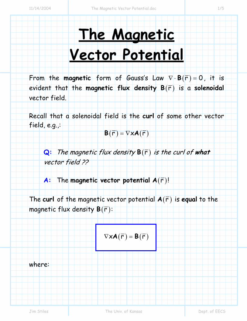
From the magnetic form of Gauss’s Law ( )r 0∇ ⋅ =B , it is evident that the magnetic flux density ( )rB is a solenoidal vector field. Recall that a solenoidal field is the curl of some other vector field, e.g.,:
( ) ( )r x r= ∇B A
Q: The magnetic flux density ( )rB is the curl of what vector field ?? A: The magnetic vector potential ( )rA !
The curl of the magnetic vector potential ( )rA is equal to the magnetic flux density ( )rB :
( ) ( )x r r∇ =A B
where:
11/14/2004 The Magnetic Vector Potential.doc 2/5
Jim Stiles The Univ. of Kansas Dept. of EECS
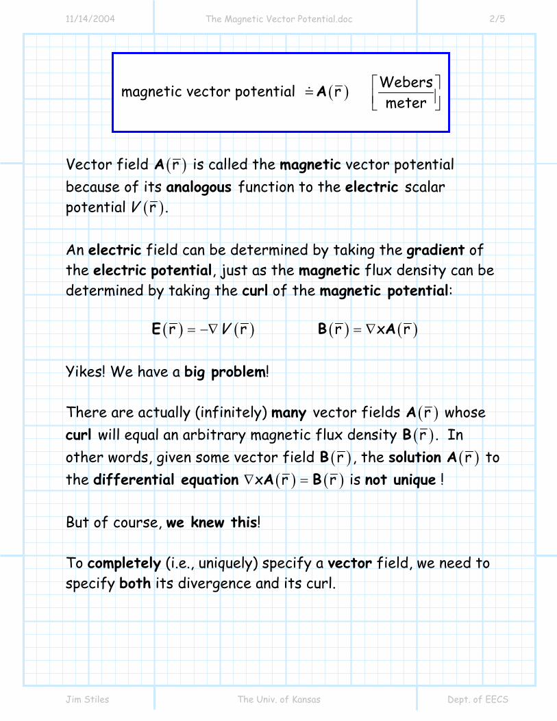
( ) Webersmagnetic vector potential r meter
⎡ ⎤⎢ ⎥⎣ ⎦
A
Vector field ( )rA is called the magnetic vector potential because of its analogous function to the electric scalar potential ( )rV . An electric field can be determined by taking the gradient of the electric potential, just as the magnetic flux density can be determined by taking the curl of the magnetic potential:
( ) ( ) ( ) ( )r r r x rV= −∇ = ∇E B A
Yikes! We have a big problem! There are actually (infinitely) many vector fields ( )rA whose curl will equal an arbitrary magnetic flux density ( )rB . In other words, given some vector field ( )rB , the solution ( )rA to the differential equation ( ) ( )x r r∇ =A B is not unique ! But of course, we knew this! To completely (i.e., uniquely) specify a vector field, we need to specify both its divergence and its curl.
11/14/2004 The Magnetic Vector Potential.doc 3/5
Jim Stiles The Univ. of Kansas Dept. of EECS
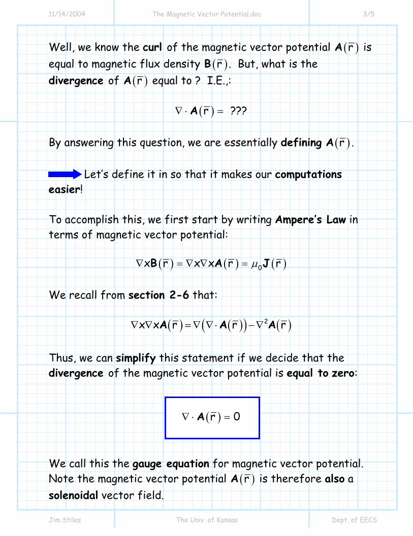
Well, we know the curl of the magnetic vector potential ( )rA is equal to magnetic flux density ( )rB . But, what is the divergence of ( )rA equal to ? I.E.,:
( )r ???∇ ⋅ =A
By answering this question, we are essentially defining ( )rA . Let’s define it in so that it makes our computations easier! To accomplish this, we first start by writing Ampere’s Law in terms of magnetic vector potential:
( ) ( ) ( )0x r x x r rµ∇ = ∇ ∇ =B A J
We recall from section 2-6 that:
( ) ( )( ) ( )2x x r r r∇ ∇ = ∇ ∇ ⋅ −∇A A A
Thus, we can simplify this statement if we decide that the divergence of the magnetic vector potential is equal to zero:
( )r 0∇ ⋅ =A
We call this the gauge equation for magnetic vector potential. Note the magnetic vector potential ( )rA is therefore also a solenoidal vector field.
11/14/2004 The Magnetic Vector Potential.doc 4/5
Jim Stiles The Univ. of Kansas Dept. of EECS
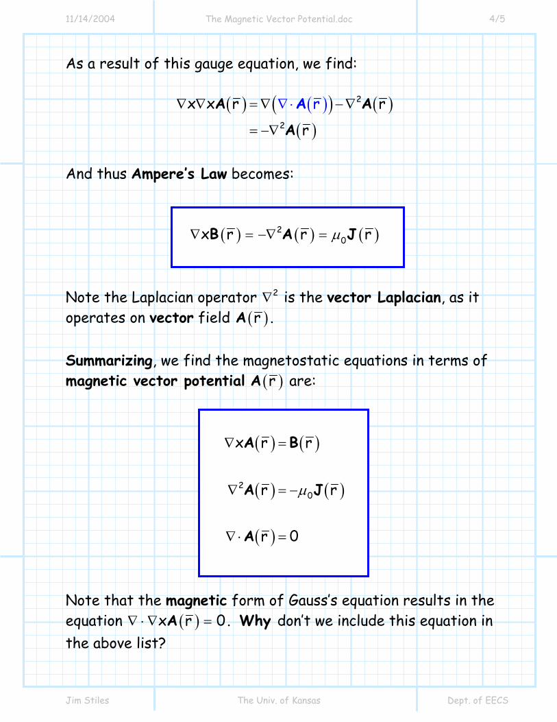
As a result of this gauge equation, we find:
( ) ( )( ) ( )( )
2
2
rx x r r
r
∇ ∇ = ∇ −∇
= −
⋅
∇
∇ AAA
A
And thus Ampere’s Law becomes:
( ) ( ) ( )20x r r rµ∇ = −∇ =B A J
Note the Laplacian operator 2∇ is the vector Laplacian, as it operates on vector field ( )rA .
Summarizing, we find the magnetostatic equations in terms of magnetic vector potential ( )rA are:
( ) ( )
( ) ( )
( )
20
x r r
r r
r 0
µ
∇ =
∇ = −
∇ ⋅ =
A B
A J
A
Note that the magnetic form of Gauss’s equation results in the equation ( )x r 0∇ ⋅∇ =A . Why don’t we include this equation in the above list?
11/14/2004 The Magnetic Vector Potential.doc 5/5
Jim Stiles The Univ. of Kansas Dept. of EECS
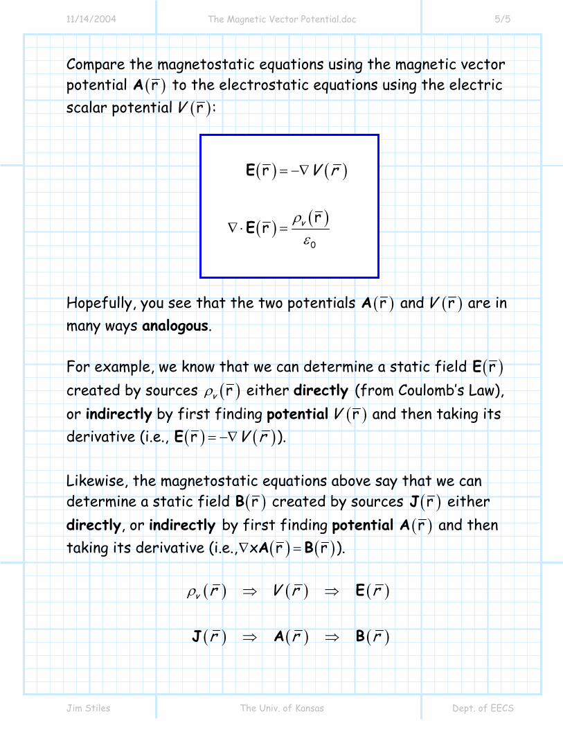
Compare the magnetostatic equations using the magnetic vector potential ( )rA to the electrostatic equations using the electric scalar potential ( )rV :
( ) ( )
( ) ( )0
r
rr v
V r
ρε
= −∇
∇ ⋅ =
E
E
Hopefully, you see that the two potentials ( )rA and ( )rV are in many ways analogous. For example, we know that we can determine a static field ( )rE created by sources ( )rvρ either directly (from Coulomb’s Law), or indirectly by first finding potential ( )rV and then taking its derivative (i.e., ( ) ( )r V r= −∇E ). Likewise, the magnetostatic equations above say that we can determine a static field ( )rB created by sources ( )rJ either directly, or indirectly by first finding potential ( )rA and then taking its derivative (i.e., ( ) ( )x r r∇ =A B ).
( ) ( ) ( )
( ) ( ) ( )
v r V r r
r r r
ρ ⇒ ⇒
⇒ ⇒
E
J A B
11/14/2004 Solutions to Amperes Law.doc 1/4
Jim Stiles The Univ. of Kansas Dept. of EECS
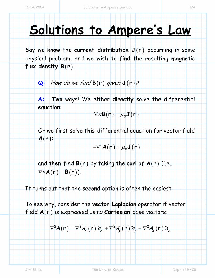
Solutions to Ampere’s Law Say we know the current distribution ( )rJ occurring in some physical problem, and we wish to find the resulting magnetic flux density ( )rB .
Q: How do we find ( )rB given ( )rJ ? A: Two ways! We either directly solve the differential equation:
( ) ( )0x r rµ∇ =B J
Or we first solve this differential equation for vector field ( )rA :
( ) ( )20r rµ−∇ =A J
and then find ( )rB by taking the curl of ( )rA (i.e.,
( ) ( )x r r∇ =A B ).
It turns out that the second option is often the easiest! To see why, consider the vector Laplacian operator if vector field ( )rA is expressed using Cartesian base vectors:
( ) ( ) ( ) ( )2 2 2 2r r r rˆ ˆ ˆx x y y z zA a A a A a∇ = ∇ + ∇ + ∇A
11/14/2004 Solutions to Amperes Law.doc 2/4
Jim Stiles The Univ. of Kansas Dept. of EECS
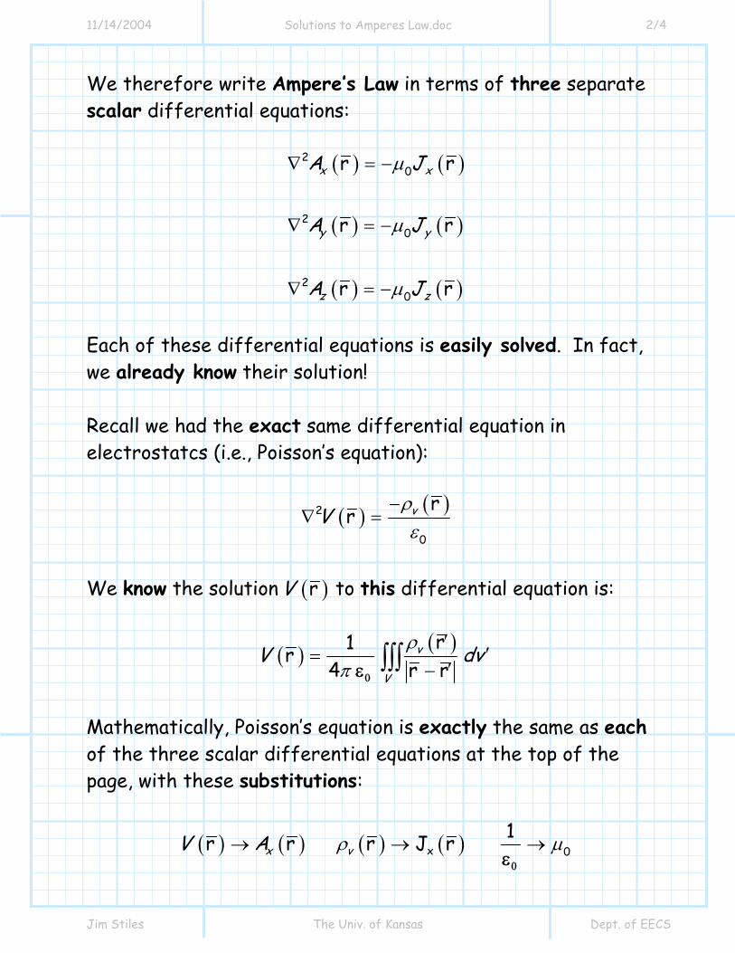
We therefore write Ampere’s Law in terms of three separate scalar differential equations:
( ) ( )
( ) ( )
( ) ( )
20
20
20
r r
r r
r r
x x
y y
z z
A J
A J
A J
µ
µ
µ
∇ = −
∇ = −
∇ = −
Each of these differential equations is easily solved. In fact, we already know their solution! Recall we had the exact same differential equation in electrostatcs (i.e., Poisson’s equation):
( ) ( )2
0
rr vV ρε
−∇ =
We know the solution ( )rV to this differential equation is:
( ) ( )r1r4 r r
v
VV dvρ
π′
′=′−∫∫∫
0ε
Mathematically, Poisson’s equation is exactly the same as each of the three scalar differential equations at the top of the page, with these substitutions:
( ) ( ) ( ) ( )x 01r r r J r x vV A ρ µ→ → →0ε
11/14/2004 Solutions to Amperes Law.doc 3/4
Jim Stiles The Univ. of Kansas Dept. of EECS
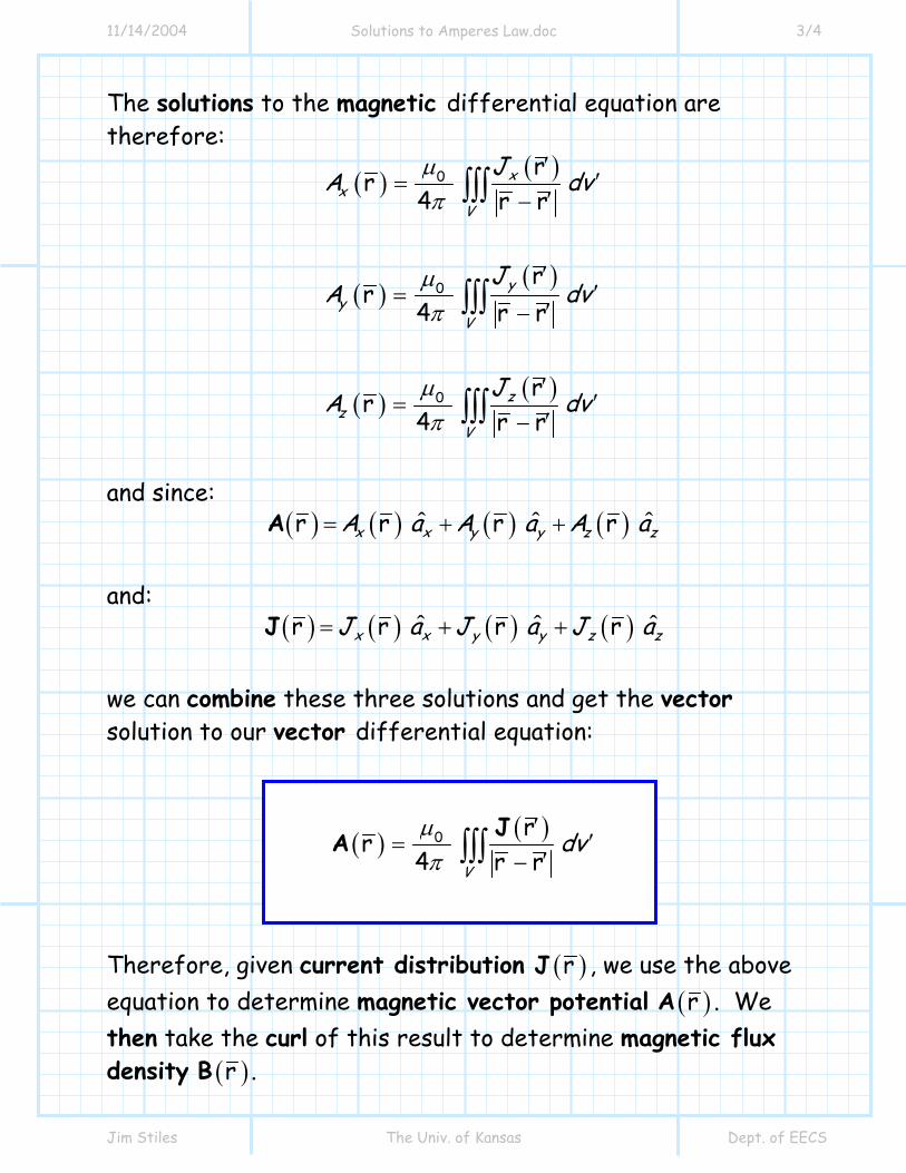
The solutions to the magnetic differential equation are therefore:
( ) ( )
( )( )
( ) ( )
0
0
0
rr4 r r
rr
4 r r
rr4 r r
xx
V
yy
V
zz
V
JA dv
JA dv
JA dv
µπ
µπ
µπ
′′=
′−
′′=
′−
′′=
′−
∫∫∫
∫∫∫
∫∫∫
and since:
( ) ( ) ( ) ( )ˆ ˆ ˆr r r rx x y y z zA a A a A a= + +A
and: ( ) ( ) ( ) ( )ˆ ˆ ˆr r r rx x y y z zJ a J a J a= + +J
we can combine these three solutions and get the vector solution to our vector differential equation:
( ) ( )0 rr4 r rV
dvµπ
′′=
′−∫∫∫JA
Therefore, given current distribution ( )rJ , we use the above equation to determine magnetic vector potential ( )rA . We then take the curl of this result to determine magnetic flux density ( )rB .
11/14/2004 Solutions to Amperes Law.doc 4/4
Jim Stiles The Univ. of Kansas Dept. of EECS
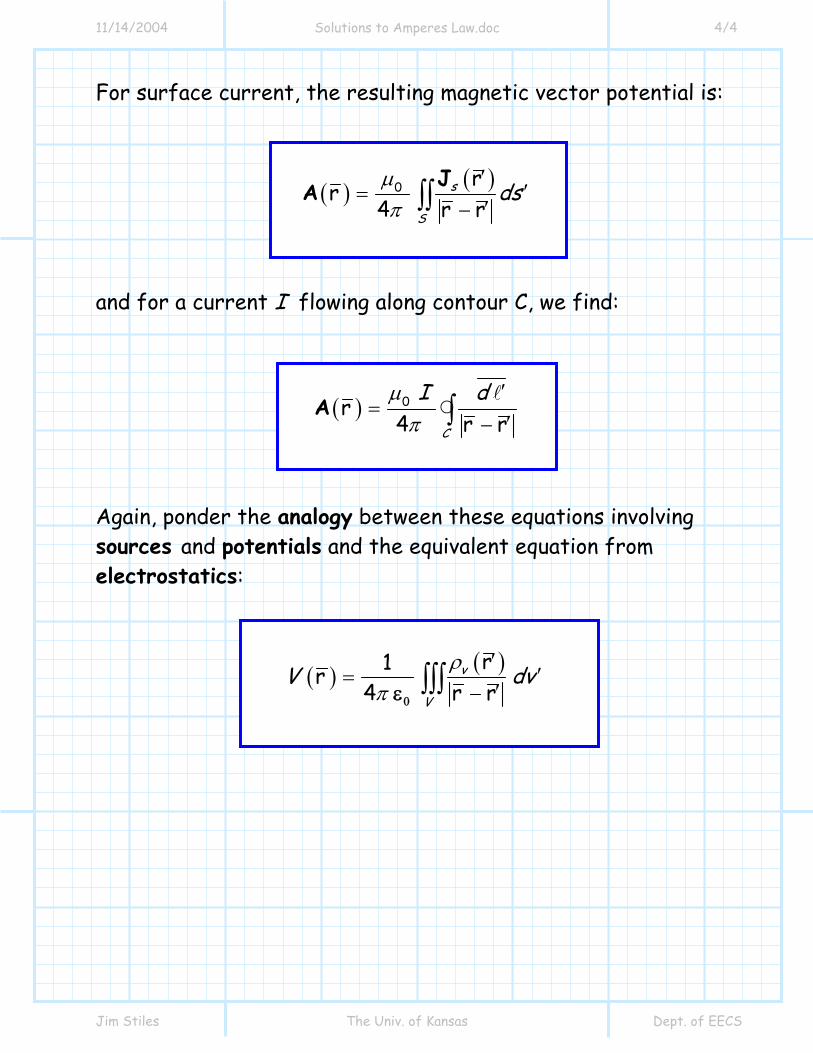
For surface current, the resulting magnetic vector potential is:
( ) ( )0 rr4 r r
s
Sdsµ
π′
′=′−∫∫
JA
and for a current I flowing along contour C, we find:
( ) 0r4 r rC
I dµπ
′=
′−∫A
Again, ponder the analogy between these equations involving sources and potentials and the equivalent equation from electrostatics:
( ) ( )r1r4 r r
v
VV dvρ
π′
′=′−∫∫∫
0ε
11/14/2004 The Biot Savart Law.doc 1/4
Jim Stiles The Univ. of Kansas Dept. of EECS
The Biot-Savart Law So, we now know that given some current density, we can find the resulting magnetic vector potential ( )rA :
( ) ( )0 rr4 r rV
dvµπ
′′=
′−∫∫∫JA
and then determine the resulting magnetic flux density ( )rB by taking the curl:
( ) ( )r x r= ∇B A
Combining the two above equations, we get:
( ) ( )0 rr x4 r rV
dvµπ
′′= ∇
′−∫∫∫JB
This result is of course not very helpful, but we note that we can move the curl operation into the integrand:
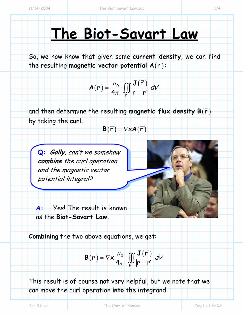
Q: Golly, can’t we somehow combine the curl operation and the magnetic vector potential integral?
A: Yes! The result is knownas the Biot-Savart Law.
11/14/2004 The Biot Savart Law.doc 2/4
Jim Stiles The Univ. of Kansas Dept. of EECS
( ) ( )0 rr x4 r rV
dvµπ
′′= ∇
′−∫∫∫JB
Note this result reverses the process: first we perform the curl, and then we integrate. We can do this is because the integral is over the primed coordinates (i.e.,r′) that specify the sources (current density), while the curl take the derivatives of the unprimed coordinates (i.e., r ) that describe the fields (magnetic flux density). Q: Yikes! That curl operation still looks particularly difficult. How we perform it? A: We take advantage of a know vector identity! The curl of vector field ( ) ( )r rf G , where ( )rf is any scalar field and ( )rG is any vector field, can be evaluated as:
( ) ( )( ) ( ) ( ) ( ) ( )x f r r r x r r x rf f∇ = ∇ − ∇G G G
Note the integrand of the above equation is in the form ( ) ( )( )x f r r∇ G , where:
( ) ( ) ( )1r and r rr r
f ′= =′−
G J
Therefore we find:
11/14/2004 The Biot Savart Law.doc 3/4
Jim Stiles The Univ. of Kansas Dept. of EECS
( ) ( ) ( )r 1 1x x r r xr r r r r r
⎛ ⎞ ⎛ ⎞′′ ′∇ = ∇ − ∇⎜ ⎟ ⎜ ⎟′ ′ ′− − −⎝ ⎠ ⎝ ⎠
J J J
In the first term we take the curl of ( )r′J . Note however that this vector field is a constant with respect to the unprimed coordinates r . Thus the derivatives in the curl will all be equal to zero, and we find that:
( )x r 0′∇ =J
Likewise, it can be shown that:
31 r r
r r r r⎛ ⎞ ′−
∇ = −⎜ ⎟′− ′−⎝ ⎠
Using these results, we find:
( ) ( ) ( )3
r r x r rxr r r r
⎛ ⎞′ ′ ′−∇ =⎜ ⎟′− ′−⎝ ⎠
J J
and therefore the magnetic flux density is:
( ) ( ) ( )03
r x r rr4 r rV
dvµπ
′ ′−′=
′−∫∫∫JB
This is know as the Biot-Savart Law !
11/14/2004 The Biot Savart Law.doc 4/4
Jim Stiles The Univ. of Kansas Dept. of EECS
For a surface current ( )rsJ , the Biot-Savart Law becomes:
( ) ( ) ( )03
r x r rr4 r r
s
S
dsµπ
′ ′−′=
′−∫∫JB
and for line current I, flowing on contour C, the Biot-Savart Law is:
( ) ( )03
x r rr4 r rC
dIµπ
′ ′−=
′−∫B
Note the contour C is closed. Do you know why?
Note that the Biot-Savart Law is therefore analogous to Coloumb’s Law in Electrostatics (Do you see why?)!
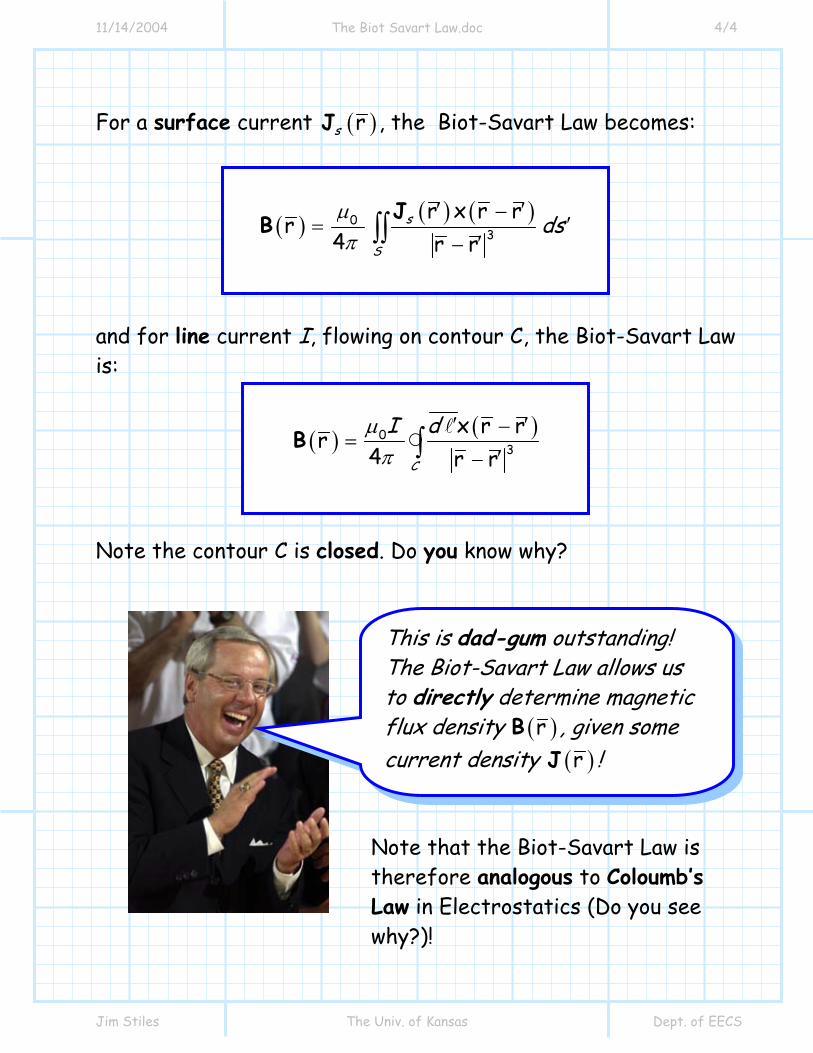
This is dad-gum outstanding! The Biot-Savart Law allows us to directly determine magnetic flux density ( )rB , given some current density ( )rJ !
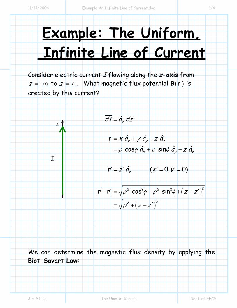
11/14/2004 Example An Infinite Line of Current.doc 1/4
Jim Stiles The Univ. of Kansas Dept. of EECS
Example: The Uniform, Infinite Line of Current
Consider electric current I flowing along the z-axis from z = −∞ to z = ∞ . What magnetic flux potential ( )rB is created by this current?
( )
( )
ˆ
ˆ ˆ ˆ
ˆ ˆ ˆ
ˆ ( , )
22 2 2 2
22
r cos sin
r 0 0
r r cos sin
z
x y z
x y z
z
d a dz
x a y a z aa a z a
z a x y
z z
z z
ρ φ ρ φ
ρ φ ρ φ
ρ
′=
= + +
= + +
′ ′ ′ ′= = =
′ ′− = + + −
′= + −
We can determine the magnetic flux density by applying the Biot-Savart Law:
z
I
11/14/2004 Example An Infinite Line of Current.doc 2/4
Jim Stiles The Univ. of Kansas Dept. of EECS
( ) ( )
( )
( )
( )
( )
( )
( )
ˆ ˆ
ˆ
ˆ ˆ ˆ ˆ
ˆ ˆ
ˆ
03
03
2 22
03
2 22
03
2 2 2
02 2 2
0
x r rr
4 r r
x cos sin4
cos s
cos s
in4
4
u
in
4 -
4
|
y x
C
z x y z
y x
dI
a a a z z aI dzz z
a aI dzz z
I duu
Iu
I a
a a
aφ
φ
µπ
ρ φ ρ φµπ ρ
ρ φ ρ φµπ ρ
µπ ρ
µπ ρ ρ
µ ρπ
ρ φ ρ φ
ρ
∞
−∞
∞
−∞
∞
−∞
′ ′−=
′−
⎡ ⎤′+ + −⎣ ⎦ ′=⎡ ⎤′+ −⎣ ⎦
−′=
⎡ ⎤′+ −⎣ ⎦
=⎡ ⎤+⎣ ⎦
∞
∞ +
=
−
=
∫
∫
∫
∫
B
ˆ
2
0
2
2I aφ
ρµπ ρ
=
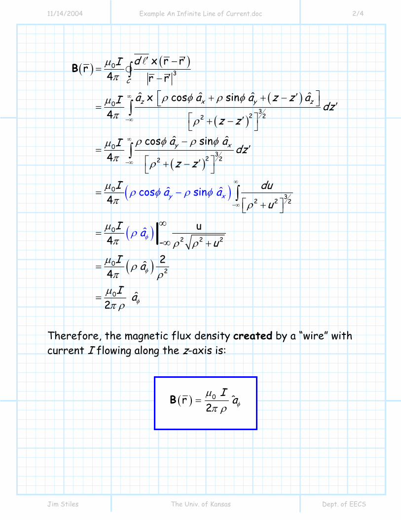
Therefore, the magnetic flux density created by a “wire” with current I flowing along the z-axis is:
( ) 0r2
ˆI aφ
µπ ρ
=B
11/14/2004 Example An Infinite Line of Current.doc 3/4
Jim Stiles The Univ. of Kansas Dept. of EECS
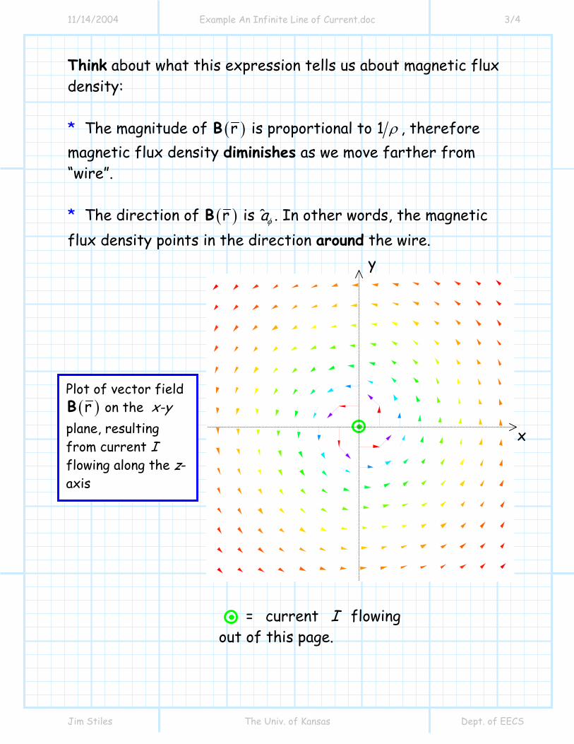
Think about what this expression tells us about magnetic flux density: * The magnitude of ( )rB is proportional to 1 ρ , therefore magnetic flux density diminishes as we move farther from “wire”. * The direction of ( )rB is aφ . In other words, the magnetic flux density points in the direction around the wire.
= current I flowingout of this page.
y
x
Plot of vector field ( )rB on the x-y
plane, resulting from current I flowing along the z-axis
11/14/2004 Example An Infinite Line of Current.doc 4/4
Jim Stiles The Univ. of Kansas Dept. of EECS
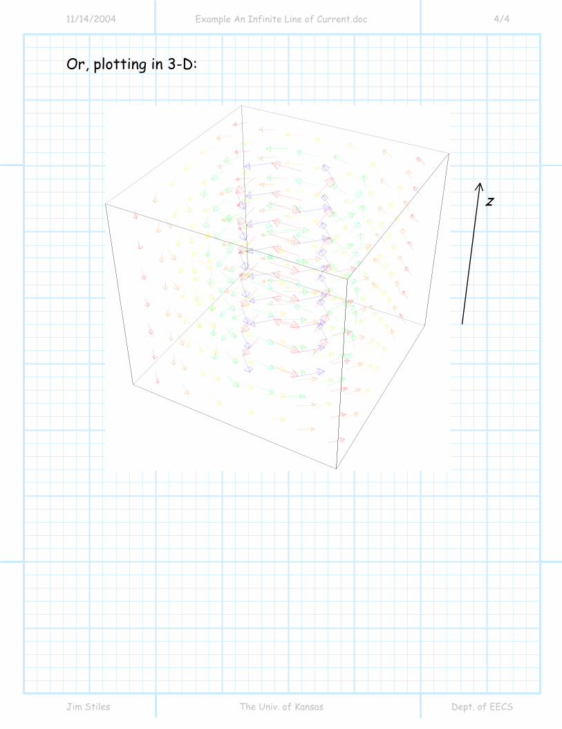
Or, plotting in 3-D:
z
11/14/2004 An Infinite Sheet of Current.doc 1/3
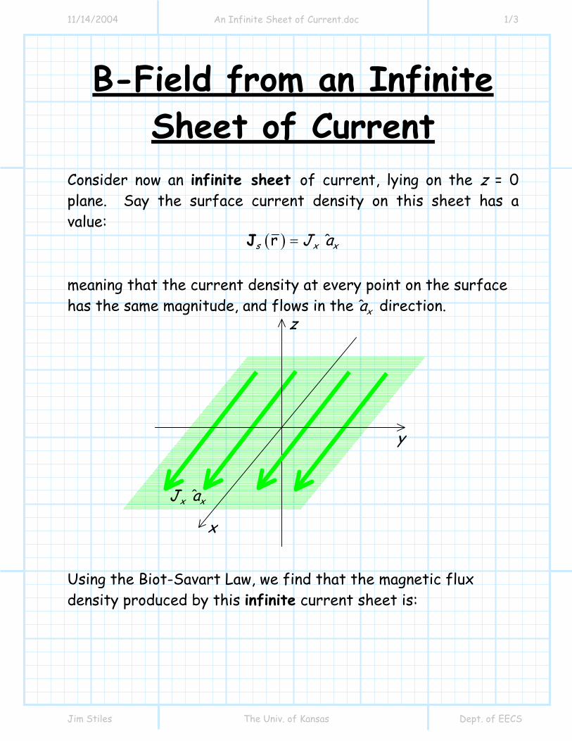
Jim Stiles The Univ. of Kansas Dept. of EECS
B-Field from an Infinite Sheet of Current
Consider now an infinite sheet of current, lying on the z = 0 plane. Say the surface current density on this sheet has a value:
( )r ˆs x xJ a=J
meaning that the current density at every point on the surface has the same magnitude, and flows in the ˆ xa direction. Using the Biot-Savart Law, we find that the magnetic flux density produced by this infinite current sheet is:
x
y
z
ˆx xJ a
11/14/2004 An Infinite Sheet of Current.doc 2/3
Jim Stiles The Univ. of Kansas Dept. of EECS
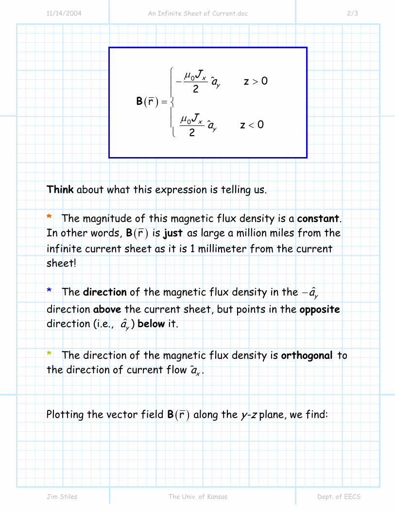
( )
0
0
z 02
r
z 02
ˆ
ˆ
xy
xy
J a
J a
µ
µ
⎧− >⎪⎪
= ⎨⎪⎪ <⎩
B
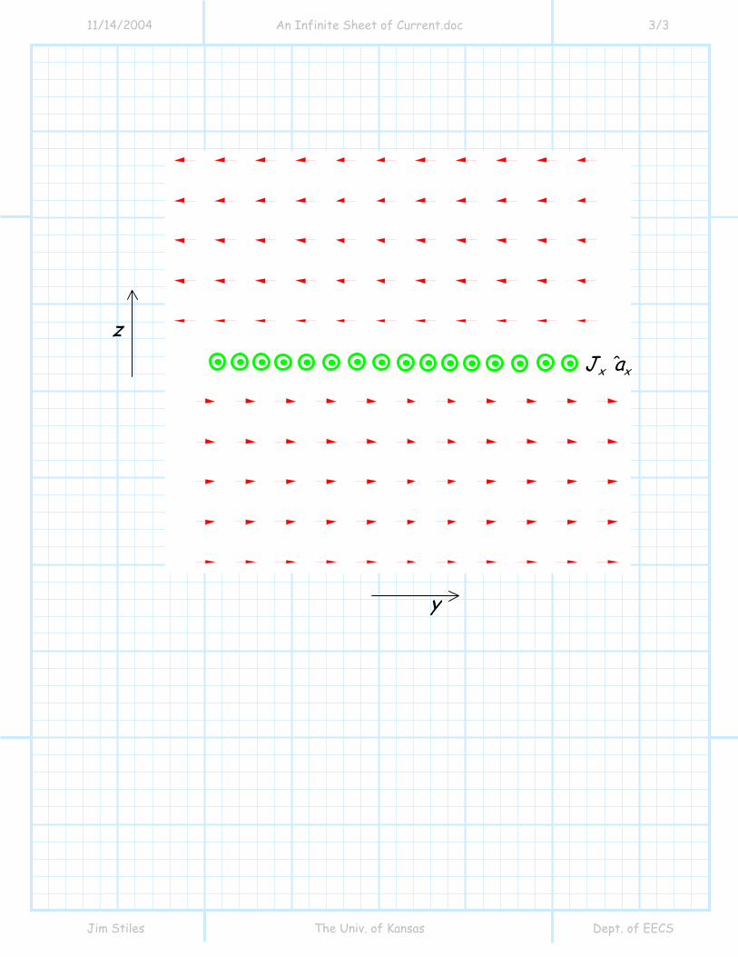
Think about what this expression is telling us. * The magnitude of this magnetic flux density is a constant. In other words, ( )rB is just as large a million miles from the infinite current sheet as it is 1 millimeter from the current sheet! * The direction of the magnetic flux density in the ya− direction above the current sheet, but points in the opposite direction (i.e., ya ) below it. * The direction of the magnetic flux density is orthogonal to the direction of current flow ˆ xa . Plotting the vector field ( )rB along the y-z plane, we find:
11/14/2004 An Infinite Sheet of Current.doc 3/3
Jim Stiles The Univ. of Kansas Dept. of EECS
z
y
ˆx xJ a