1  

Evaluation of gvSIG and SEXTANTE Tools for Hydrological Analysis

Schröder Dietricha, Mudogah Hildahb and Franz Davidb abPhotogrammetry and Geo-informatics Masters Programme, Stuttgart University of Applied

Sciences, Germany - dietrich.schroeder@hft-stuttgart.de

6th International gvSIG Conference

Key words: DEM, interpolation, hydrological modelling, viewshed analysis

1. Summary As part of the GIS training and education in the Photogrammetry and Geo-informatics Master’s program at Stuttgart University of Applied Sciences, the students have to carry out a number of studio projects. In one of these projects a hydrological analysis of a small dam project in South-West Germany has been done using gvSIG and SEXTANTE. As the study area is rather homogeneous, a simple model for infiltration as well as evapo-transpiration has been considered. The calculations are based on a Digital Elevation Model (DEM) created from digitized contour lines and supported by other vector and climate data. Overall, about 65 different tools or steps in gvSIG and SEXTANTE have been used in the project. About 3/4 of the tools worked without any problems. For about 5 % of the tasks no explicit tools have been found, while the rest accounts for workarounds that have been used.

2. Introduction In the context of sustainable development the share of renewable energy, e.g. water energy, should be increased. In a small valley of the Black Forest in the 1920’s a dam was built for water energy production, but the plant was shut down in the 1960’s. Now there is a discussion to revive the dam, or even to build a higher dam. In the planning, issues such as flood protection as well as landscape preservation have to be considered since the area is part of the nature reserve of the southern Black Forest. For this reason, the planning authority of the project requires several calculations to be made and some maps to be prepared.

For a complete GIS-based hydrological analysis, numerous steps have to be carried out based on vector as well as raster data. Based on the DEM, sink filling, flow accumulation, as well as channel network and watershed delineation tools from SEXTANTE have been used. To calculate the surface run-off and the unit hydrograph, interpolation of rain-fall data from climate stations has been done. For the unit hydrograph, the flow time for each raster pixel to the outlet point which is the dam location, has been calculated. The velocity raster is based on the roughness of the terrain extracted from a land cover layer and the slope is derived from the DEM. In addition, the storage capacity for the planned dam has been calculated based on the DEM. In the final step, a view shed analysis for the dam location is done.

While most of the tools run without problems, some of them have not worked as expected. In particular, there have been several problems in the raster analysis part of the project, for instance the NoData problem has caused a lot of trouble. Thus some suggestions for improvement can be extracted from this study.

Initially, the main work of the studio project has been done using gvSIG 1.9 and OADE 2010 version. Some of the steps which caused problems have been repeated recently using gvSIG 1.10. In this study the necessary steps as well as the corresponding tools are discussed.

 

The dat

DaDEClRiRaCOLa

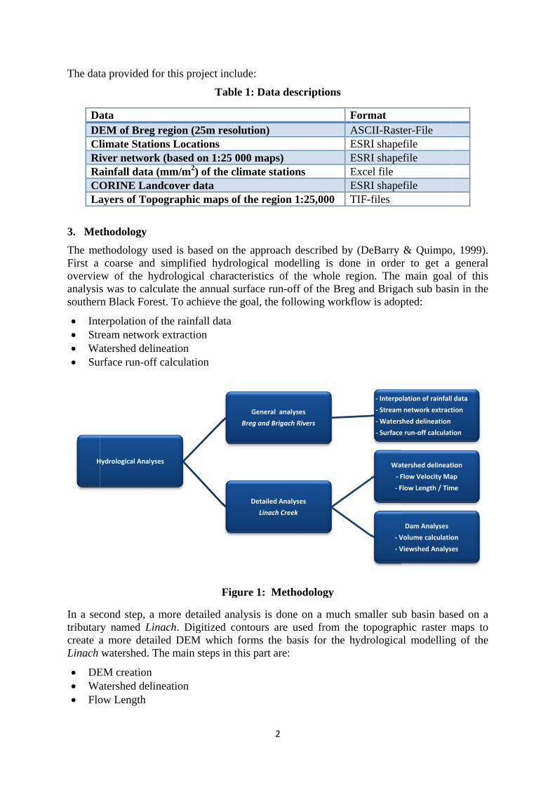
3. Met

The meFirst a overvieanalysissouther

• Int• Str• Wa• Sur

In a sectributarcreate aLinach

• DE• Wa• Flo

H

ta provided

ata EM of Breglimate Stativer networainfall dataORINE Laayers of To

thodology

ethodology coarse and

ew of the hs was to caln Black For

terpolation oream networatershed delrface run-of

cond step, ay named La more detawatershed.

EM creationatershed delow Length

Hydrological Anal

for this proj

g region (25tions Locatirk (based oa (mm/m2) andcover daopographic

used is basd simplifiehydrologicalculate the arest. To ach

of the rainfark extractiolineation ff calculatio

a more detaLinach. Digailed DEMThe main s

n lineation

yses

oject include

Table 1

5m resolutions

on 1:25 000of the climata maps of th

sed on the ad hydrolog

al characterannual surfa

hieve the go

all data on

on

Figure

ailed analysgitized conto which form

steps in this

Bre

2 

e:

: Data desc

tion)

0 maps) mate station

he region 1

approach dgical modelristics of thface run-off al, the follo

e 1: Metho

sis is done ours are usms the baspart are:

General  analyse

eg and Brigach Ri

Detailed Analyse

Linach Creek

criptions

FAEE

s EE

:25,000 T

escribed bylling is donhe whole ref of the Bregowing workf

odology

on a much sed from this for the h

es 

ivers

es

FormatASCII-RastESRI shapeESRI shapeExcel file ESRI shapeTIF-files

y (DeBarry ne in orderegion. The g and Brigaflow is adop

smaller suhe topographydrologica

‐ Interpo

‐ Stream

‐Waters

‐ Surface

Wa

‐ F

‐ F

‐ V

‐ V

ter-File efile efile

efile

& Quimpor to get a main goal

ach sub basipted:

ub basin basphic raster mal modelling

olation of rainfall

m network extract

shed delineation

e run‐off calculat

tershed delineat

Flow Velocity Ma

Flow Length / Tim

Dam Analyses

Volume calculatio

Viewshed Analys

o, 1999). general

l of this in in the

sed on a maps to g of the

l data

tion

ion

tion

ap

me

on

es

3  

• Flow Velocity and Flow time calculations • Volume calculations • Viewshed analysis

4. General hydrological analysis for Breg and Brigach rivers

The Breg is a river in Baden-Württemberg, Germany, with its source in the Black Forest. It joins with the second headstream, the river Brigach, to form the river Danube. For the sub-basins of Breg and Brigach, watershed delineation, drainage map preparation, stream network extraction and surface run-off computations are done. The study area has an extent of approximately 40 x 55 km2. For all raster calculations, a fixed resolution defined by the given DEM of 25 x 25 m has been used. Thus the created rasters have about 1600 x 2200 cells.

Since annual precipitation would be necessary for calculating surface runoff, the provided rainfall data was transformed to (.dbf) format and joined to the climate stations locations table. For the study area the data of 16 stations were available. Various interpolation techniques were then tested on the joined table, based on the annual rainfall field including the Inverse Distance Weighted (IDW), Kriging, and Nearest Neighbour methods incorporated in SEXTANTE. The results of the interpolations have been compared with the output of a proprietary GIS product. As usual for a sparse data problem, several parameter settings were tested to get meaningful results. The IDW shows the typical bulls-eye effect. Nevertheless, a comparison with the results used as reference, show very small differences. To fix the parameter for Kriging, first the Spatial autocorrelation tool has been used. To fix the nugget, sill, and range parameters, the autocorrelation point cloud is exported to some external tool, since up to now no tool is available in gvSIG and SEXTANTE to calculate a theoretical semivariogram function. Using the same values for the semivariogram, the comparison with the reference dataset shows some higher differences than IDW, but the results with only a maximum difference of 5% are still comparable. As expected, the Kriging shows a much smoother distribution of the interpolated values than IDW. Thus it was used for further analysis.

The workflow for watershed delineation is based on the descriptions in (Maidment & Djokic, 2000). For the stream network extraction, the flow accumulation based on a DEM with filled sinks and pits has to be used. Unfortunately, the SEXTANTE Sink Filling and Flow Accumulation tools could not be successfully applied on this dataset. Either the algorithm didn’t stop or it came up with some generic error message. Increasing the heap size or reducing the cell resolution by resampling didn’t improve the results. With the new SEXTANTE versions a work around can be used, that is using SEXTANTE as front end for the GRASS tools. After configuring SEXTANTE for GRASS, the use of the tools is very simple.

It is well known, that calculating the flow accumulation layer to extract the drainage network may fail in flat areas. An initial calculation shows a shift between the calculated streams and the provided streams by a maximum of 800 meter for flat areas near the junction of Breg and Brigach. To improve the results, an approach dubbed “burn-in” has been applied. It involves reducing the DEM along the river trenches by a defined value and using the output as the basis of the hydrological analysis. To initiate this process, the provided data was scaled to the same extent as the provided DEM. The rivers were then buffered using the Fixed Distance Buffer tool by a distance of 12.5m for both inner and outer buffers. Within an edit session, a field was added to the attribute table of the buffered rivers. The field was populated with the value by which the DEM would be reduced, here taken as 5 metres. Using the Rasterize

4  

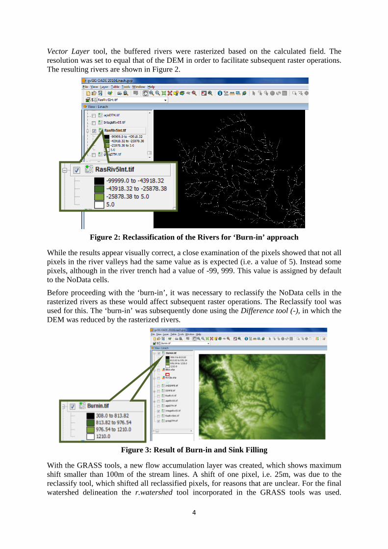
Vector Layer tool, the buffered rivers were rasterized based on the calculated field. The resolution was set to equal that of the DEM in order to facilitate subsequent raster operations. The resulting rivers are shown in Figure 2.

 

Figure 2: Reclassification of the Rivers for ‘Burn-in’ approach

While the results appear visually correct, a close examination of the pixels showed that not all pixels in the river valleys had the same value as is expected (i.e. a value of 5). Instead some pixels, although in the river trench had a value of -99, 999. This value is assigned by default to the NoData cells.

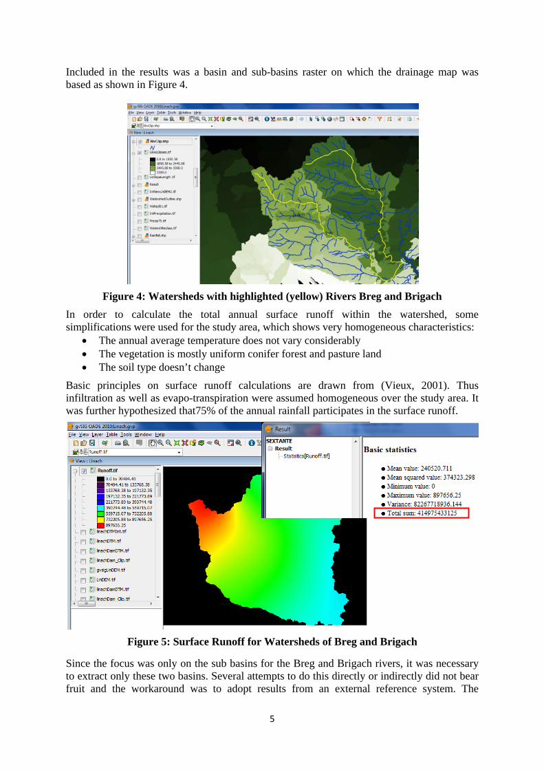
Before proceeding with the ‘burn-in’, it was necessary to reclassify the NoData cells in the rasterized rivers as these would affect subsequent raster operations. The Reclassify tool was used for this. The ‘burn-in’ was subsequently done using the Difference tool (-), in which the DEM was reduced by the rasterized rivers.

 

Figure 3: Result of Burn-in and Sink Filling

With the GRASS tools, a new flow accumulation layer was created, which shows maximum shift smaller than 100m of the stream lines. A shift of one pixel, i.e. 25m, was due to the reclassify tool, which shifted all reclassified pixels, for reasons that are unclear. For the final watershed delineation the r.watershed tool incorporated in the GRASS tools was used.

 

 

5  

Included in the results was a basin and sub-basins raster on which the drainage map was based as shown in Figure 4.

 

Figure 4: Watersheds with highlighted (yellow) Rivers Breg and Brigach In order to calculate the total annual surface runoff within the watershed, some simplifications were used for the study area, which shows very homogeneous characteristics:

• The annual average temperature does not vary considerably • The vegetation is mostly uniform conifer forest and pasture land • The soil type doesn’t change

Basic principles on surface runoff calculations are drawn from (Vieux, 2001). Thus infiltration as well as evapo-transpiration were assumed homogeneous over the study area. It was further hypothesized that75% of the annual rainfall participates in the surface runoff.

Figure 5: Surface Runoff for Watersheds of Breg and Brigach

Since the focus was only on the sub basins for the Breg and Brigach rivers, it was necessary to extract only these two basins. Several attempts to do this directly or indirectly did not bear fruit and the workaround was to adopt results from an external reference system. The

6  

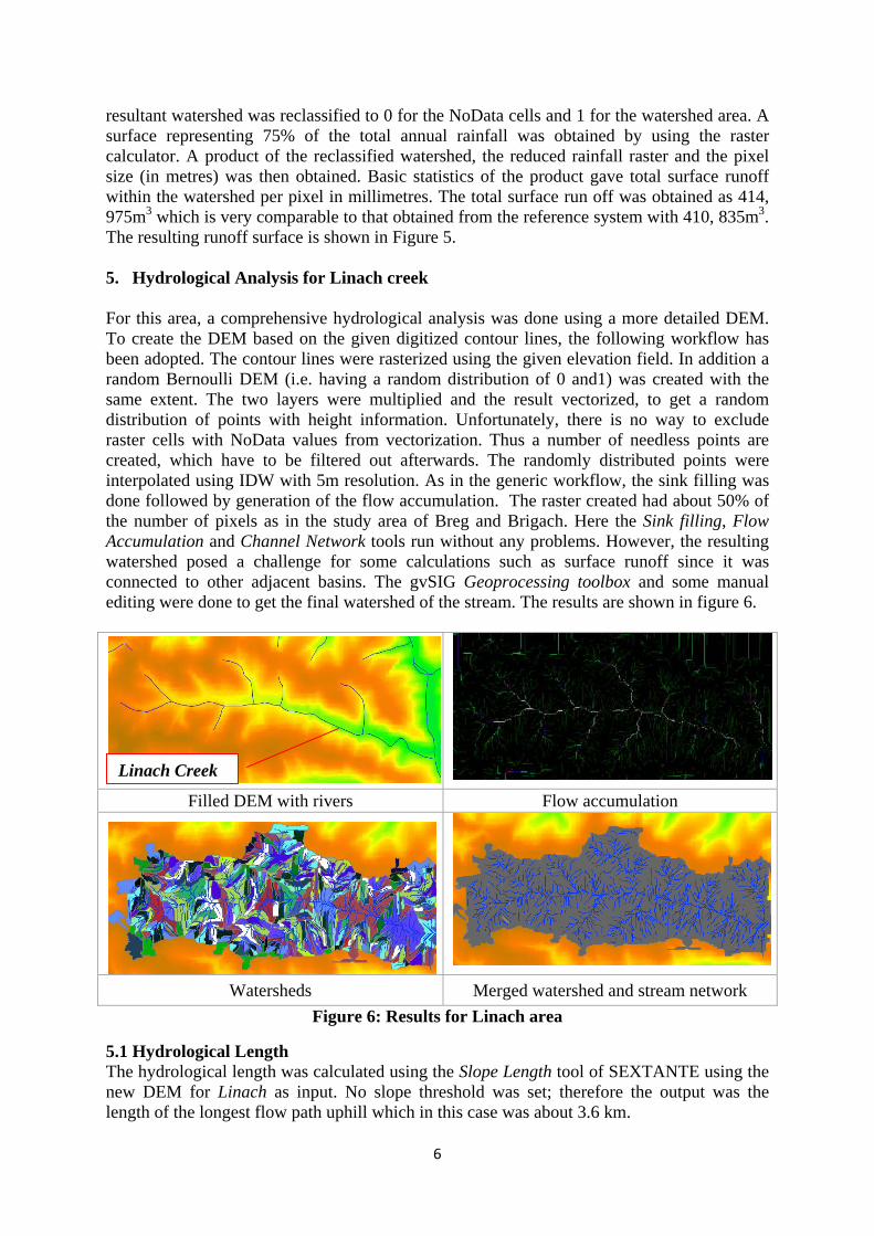
resultant watershed was reclassified to 0 for the NoData cells and 1 for the watershed area. A surface representing 75% of the total annual rainfall was obtained by using the raster calculator. A product of the reclassified watershed, the reduced rainfall raster and the pixel size (in metres) was then obtained. Basic statistics of the product gave total surface runoff within the watershed per pixel in millimetres. The total surface run off was obtained as 414, 975m3 which is very comparable to that obtained from the reference system with 410, 835m3. The resulting runoff surface is shown in Figure 5. 5. Hydrological Analysis for Linach creek For this area, a comprehensive hydrological analysis was done using a more detailed DEM. To create the DEM based on the given digitized contour lines, the following workflow has been adopted. The contour lines were rasterized using the given elevation field. In addition a random Bernoulli DEM (i.e. having a random distribution of 0 and1) was created with the same extent. The two layers were multiplied and the result vectorized, to get a random distribution of points with height information. Unfortunately, there is no way to exclude raster cells with NoData values from vectorization. Thus a number of needless points are created, which have to be filtered out afterwards. The randomly distributed points were interpolated using IDW with 5m resolution. As in the generic workflow, the sink filling was done followed by generation of the flow accumulation. The raster created had about 50% of the number of pixels as in the study area of Breg and Brigach. Here the Sink filling, Flow Accumulation and Channel Network tools run without any problems. However, the resulting watershed posed a challenge for some calculations such as surface runoff since it was connected to other adjacent basins. The gvSIG Geoprocessing toolbox and some manual editing were done to get the final watershed of the stream. The results are shown in figure 6.

Filled DEM with rivers Flow accumulation

Watersheds Merged watershed and stream network Figure 6: Results for Linach area

5.1 Hydrological Length The hydrological length was calculated using the Slope Length tool of SEXTANTE using the new DEM for Linach as input. No slope threshold was set; therefore the output was the length of the longest flow path uphill which in this case was about 3.6 km.

Linach Creek

7  

 

Figure 7: Result of Slope Length

5.2 Velocity map The flow time depends on the distance, but as well on the roughness of the surface and the slope. If a velocity map is provided as weight map to the slope length calculation, the flow time can be calculated. Unfortunately, the slope length tool of SEXTANTE doesn’t offer this option. To get an idea about the characteristics of the sub basin, a velocity map was calculated nevertheless. To calculate the flow velocity for each cell the Manning - Strickler equation can be used:

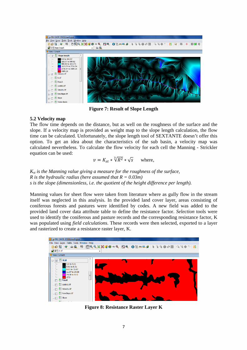
√ √ where, Kst is the Manning value giving a measure for the roughness of the surface, R is the hydraulic radius (here assumed that R = 0.03m) s is the slope (dimensionless, i.e. the quotient of the height difference per length). Manning values for sheet flow were taken from literature where as gully flow in the stream itself was neglected in this analysis. In the provided land cover layer, areas consisting of coniferous forests and pastures were identified by codes. A new field was added to the provided land cover data attribute table to define the resistance factor. Selection tools were used to identify the coniferous and pasture records and the corresponding resistance factor, K was populated using field calculations. These records were then selected, exported to a layer and rasterized to create a resistance raster layer, K.

 

Figure 8: Resistance Raster Layer K

8  

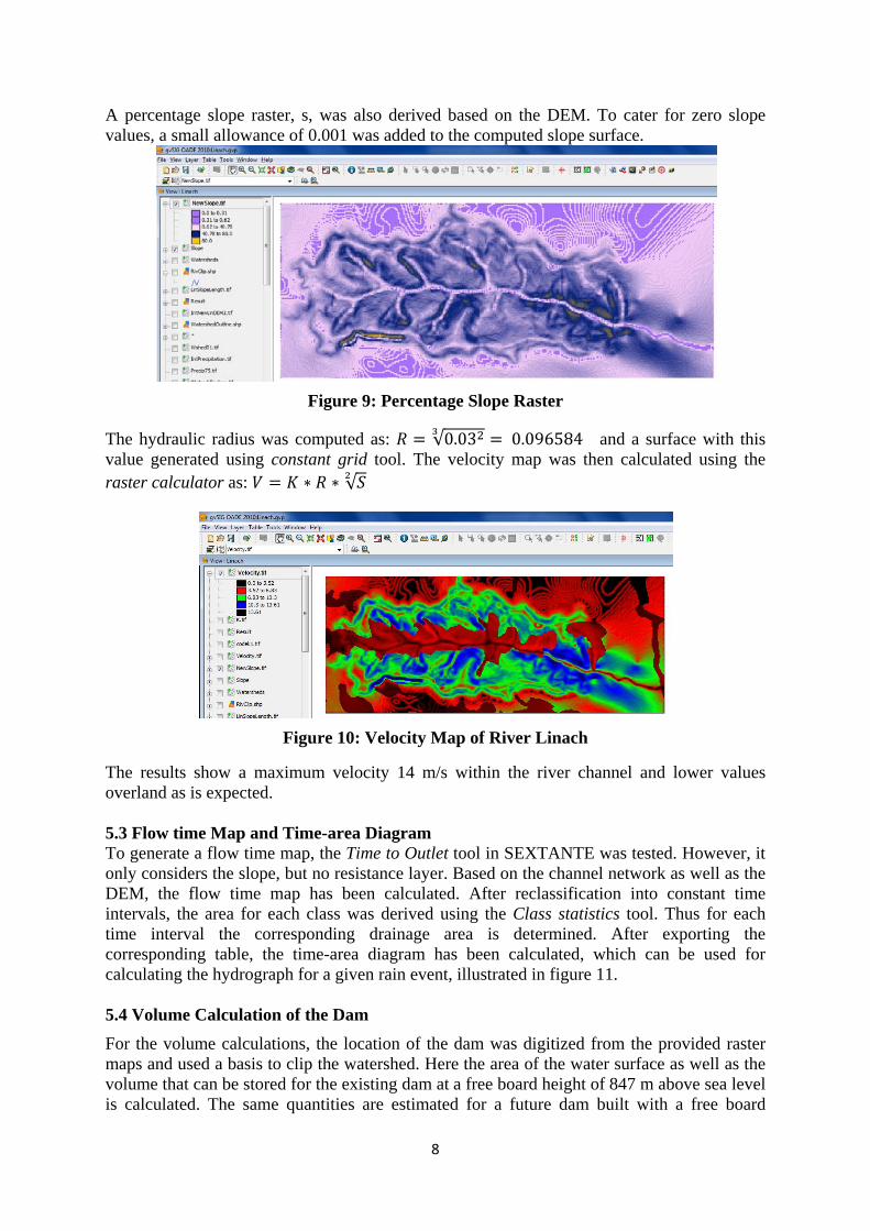
A percentage slope raster, s, was also derived based on the DEM. To cater for zero slope values, a small allowance of 0.001 was added to the computed slope surface.

 

Figure 9: Percentage Slope Raster

The hydraulic radius was computed as: √0.03 0.096584 and a surface with this value generated using constant grid tool. The velocity map was then calculated using the raster calculator as: √

 

Figure 10: Velocity Map of River Linach

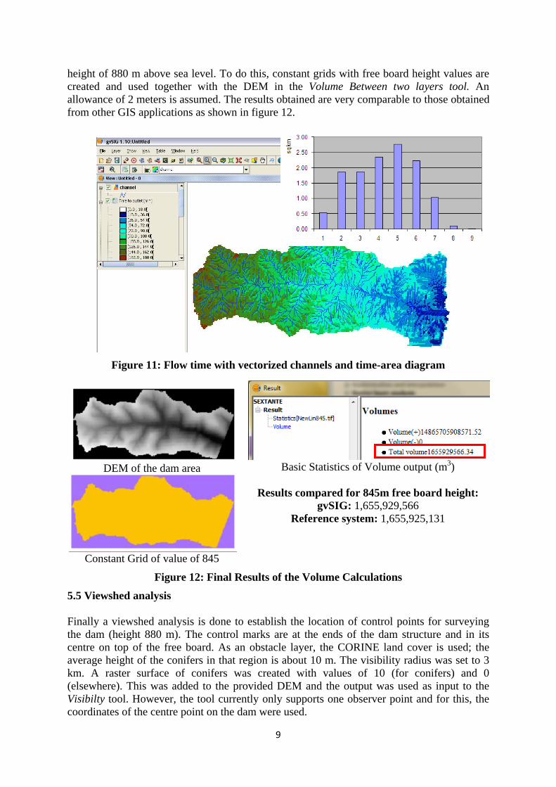
The results show a maximum velocity 14 m/s within the river channel and lower values overland as is expected. 5.3 Flow time Map and Time-area Diagram To generate a flow time map, the Time to Outlet tool in SEXTANTE was tested. However, it only considers the slope, but no resistance layer. Based on the channel network as well as the DEM, the flow time map has been calculated. After reclassification into constant time intervals, the area for each class was derived using the Class statistics tool. Thus for each time interval the corresponding drainage area is determined. After exporting the corresponding table, the time-area diagram has been calculated, which can be used for calculating the hydrograph for a given rain event, illustrated in figure 11.

5.4 Volume Calculation of the Dam

For the volume calculations, the location of the dam was digitized from the provided raster maps and used a basis to clip the watershed. Here the area of the water surface as well as the volume that can be stored for the existing dam at a free board height of 847 m above sea level is calculated. The same quantities are estimated for a future dam built with a free board

9  

height of 880 m above sea level. To do this, constant grids with free board height values are created and used together with the DEM in the Volume Between two layers tool. An allowance of 2 meters is assumed. The results obtained are very comparable to those obtained from other GIS applications as shown in figure 12.

Figure 11: Flow time with vectorized channels and time-area diagram

DEM of the dam area

Constant Grid of value of 845

Basic Statistics of Volume output (m3)

Results compared for 845m free board height: gvSIG: 1,655,929,566

Reference system: 1,655,925,131  

Figure 12: Final Results of the Volume Calculations

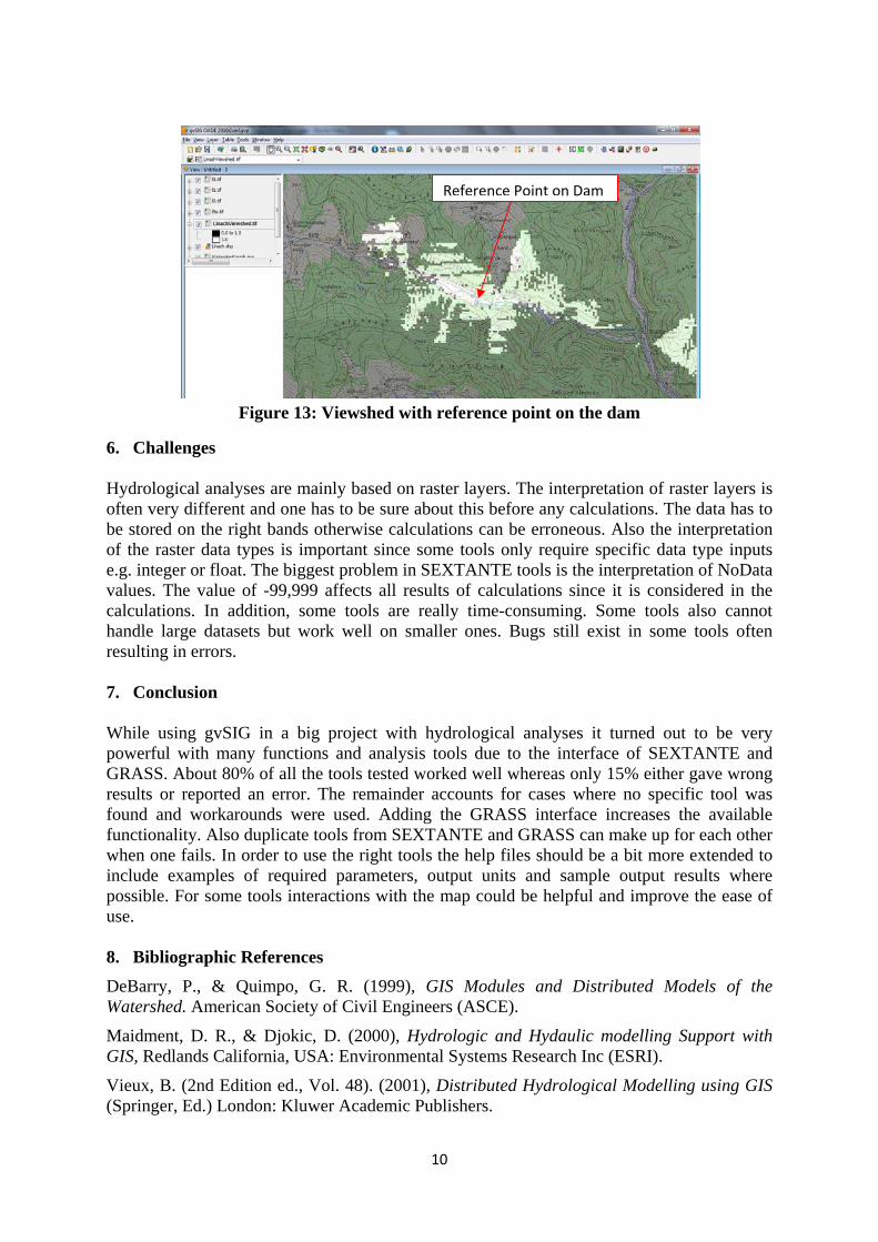
5.5 Viewshed analysis

Finally a viewshed analysis is done to establish the location of control points for surveying the dam (height 880 m). The control marks are at the ends of the dam structure and in its centre on top of the free board. As an obstacle layer, the CORINE land cover is used; the average height of the conifers in that region is about 10 m. The visibility radius was set to 3 km. A raster surface of conifers was created with values of 10 (for conifers) and 0 (elsewhere). This was added to the provided DEM and the output was used as input to the Visibilty tool. However, the tool currently only supports one observer point and for this, the coordinates of the centre point on the dam were used.

10  

 Figure 13: Viewshed with reference point on the dam

6. Challenges

Hydrological analyses are mainly based on raster layers. The interpretation of raster layers is often very different and one has to be sure about this before any calculations. The data has to be stored on the right bands otherwise calculations can be erroneous. Also the interpretation of the raster data types is important since some tools only require specific data type inputs e.g. integer or float. The biggest problem in SEXTANTE tools is the interpretation of NoData values. The value of -99,999 affects all results of calculations since it is considered in the calculations. In addition, some tools are really time-consuming. Some tools also cannot handle large datasets but work well on smaller ones. Bugs still exist in some tools often resulting in errors. 7. Conclusion

While using gvSIG in a big project with hydrological analyses it turned out to be very powerful with many functions and analysis tools due to the interface of SEXTANTE and GRASS. About 80% of all the tools tested worked well whereas only 15% either gave wrong results or reported an error. The remainder accounts for cases where no specific tool was found and workarounds were used. Adding the GRASS interface increases the available functionality. Also duplicate tools from SEXTANTE and GRASS can make up for each other when one fails. In order to use the right tools the help files should be a bit more extended to include examples of required parameters, output units and sample output results where possible. For some tools interactions with the map could be helpful and improve the ease of use. 8. Bibliographic References DeBarry, P., & Quimpo, G. R. (1999), GIS Modules and Distributed Models of the Watershed. American Society of Civil Engineers (ASCE).

Maidment, D. R., & Djokic, D. (2000), Hydrologic and Hydaulic modelling Support with GIS, Redlands California, USA: Environmental Systems Research Inc (ESRI).

Vieux, B. (2nd Edition ed., Vol. 48). (2001), Distributed Hydrological Modelling using GIS (Springer, Ed.) London: Kluwer Academic Publishers.

Reference Point on Dam