6/9/2015 Strategic Asset Allocation 1 Strategic Asset Allocation session 1 Andrei Simonov

04/18/23Strategic Asset Allocation1

Strategic Asset Allocation Strategic Asset Allocation sessionsession 1 1

Andrei Simonov


AgendaAgenda

Introduction, Course Outline, Requirements, Resources

Reminder: SAADefinitionsHistorical Records of Returns on different

securitiesCrisis in Investment Industry


Introduction Introduction The field of Finance and Investments

– Individual agents making decisions to supply capital to the markets

– Firms getting capital from the financial markets (when, where, how?)

– Capital Markets acting as market clearing device. Goal of the course:

– To familiarize you with ”real world” of investments.

– To give broad overview of modern investment issues. By June one should know what does that mean to be investment professional.


Resources and requirements:Resources and requirements: Course web page andreisimonov.com/NES Articles (package+web site)

Provide deeper insight, latest developments No econometrics, just general idea

Access to Internet, some Excel experience, basic knowledge of econometrics

It is assumed that basic courses are still remembered by you.

Groups of 2-3 (pls let TA know by the end of the week)


CasesCases What case report is NOT:

– Not copy of textbook or article.

– Not exercise in history of economics or finance. I do not care (at least, in that class) who got Nobel Prize for what...

Ideal case report is similar to consulting report:– Analysis of data that is in the case (preferrably statistical analysis)

– Covering all relevant issues (pros and cons)

– Take the position and defend it!

– Case report is not War and Peace. Be brief!

– Please understand what you are writing about.

– Cases are due before the discussion session. Do not spend more than 2 days on ANY case! Class discussion is part of the case work.


My assumptions about you:My assumptions about you:You know and understand basic regression

analysis (what is R2, statistical significance, etc.)

You remember conditions of optimality from Econ 101

You remember basics from Finance I You are willing to learn...


AgendaAgenda

Individual’s preferences, utility function Measurement of risk by variance Diversification

– A bit of math

– Industry diversification

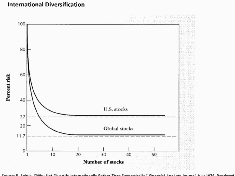
– International diversification

– Latest evidence Shortcut to math: Excel! Risk accounting


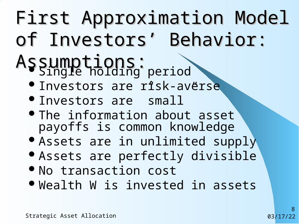
First Approximation Model of First Approximation Model of Investors’ Behavior: Assumptions:Investors’ Behavior: Assumptions:

Single holding periodInvestors are risk-averseInvestors are ”small”The information about asset payoffs is

common knowledgeAssets are in unlimited supplyAssets are perfectly divisibleNo transaction costWealth W is invested in assets


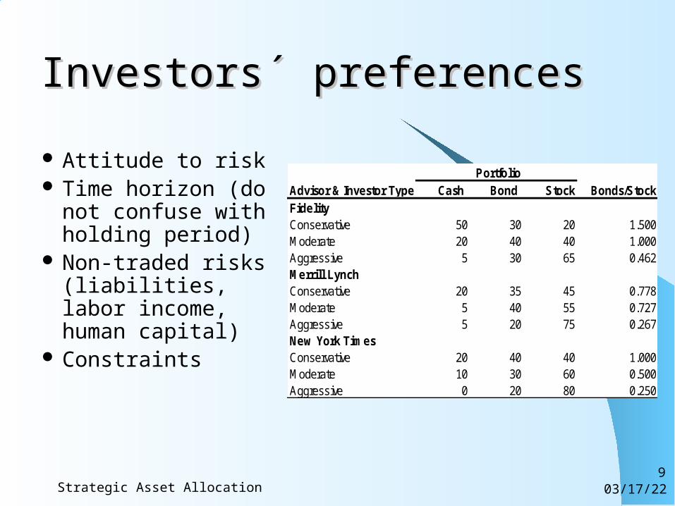
Investors´ preferencesInvestors´ preferences

Attitude to risk Time horizon (do

not confuse with holding period)

Non-traded risks (liabilities, labor income, human capital)

Constraints

PortfolioAdvisor & Investor Type: Cash Bond Stock Bonds/StockFidelityConservative 50 30 20 1.500Moderate 20 40 40 1.000Aggressive 5 30 65 0.462Merrill LynchConservative 20 35 45 0.778Moderate 5 40 55 0.727Aggressive 5 20 75 0.267New York TimesConservative 20 40 40 1.000Moderate 10 30 60 0.500Aggressive 0 20 80 0.250


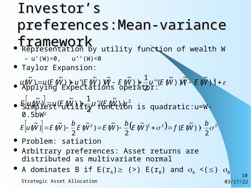
Investor’s preferences:Mean-Investor’s preferences:Mean-variance frameworkvariance framework

Representation by utility function of wealth W– u’(W)>0, u’’(W)<0

Taylor Expansion:

Applying Expectations operator:

Simplest utility function is quadratic:u=W-0.5bW2

Problem: satiation Arbitrary preferences: Asset returns are distributed as

multivariate normal A dominates B if E(rA) (>) E(rB) and A <() B

2))~

(~

))(~

((''2

1))

~(

~))(

~(('))

~(()

~( WEWWEuWEWWEuWEuWu

2))~

((''2

1))

~(()

~( WEuWEuWuE

2222

2))

~(()

~(

2)

~()

~(

2)

~()

~( b

WEfWEb

WEWEb

WEWuE


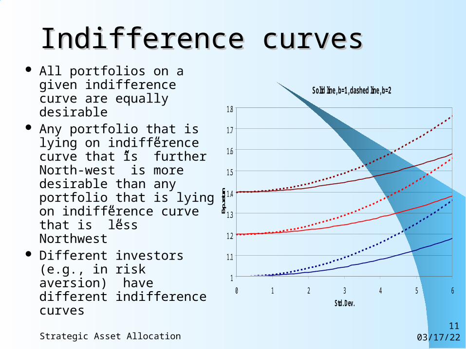
Indifference curvesIndifference curves All portfolios on a given

indifference curve are equally desirable

Any portfolio that is lying on indifference curve that is ”further North-west” is more desirable than any portfolio that is lying on indifference curve that is ”less Northwest”

Different investors (e.g., in risk aversion) have different indifference curves

Solid line, b=1, dashed line, b=2

1

1.1

1.2

1.3

1.4

1.5

1.6

1.7

1.8

0 1 2 3 4 5 6

Std. Dev.

Exp.

return


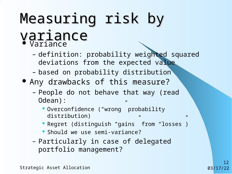
Measuring risk by varianceMeasuring risk by variance Variance

– definition: probability weighted squared deviations from the expected value

– based on probability distribution Any drawbacks of this measure?

– People do not behave that way (read Odean): Overconfidence (“wrong” probability distribution) Regret (distinguish “gains” from “losses”) Should we use semi-variance?

– Particularly in case of delegated portfolio management?


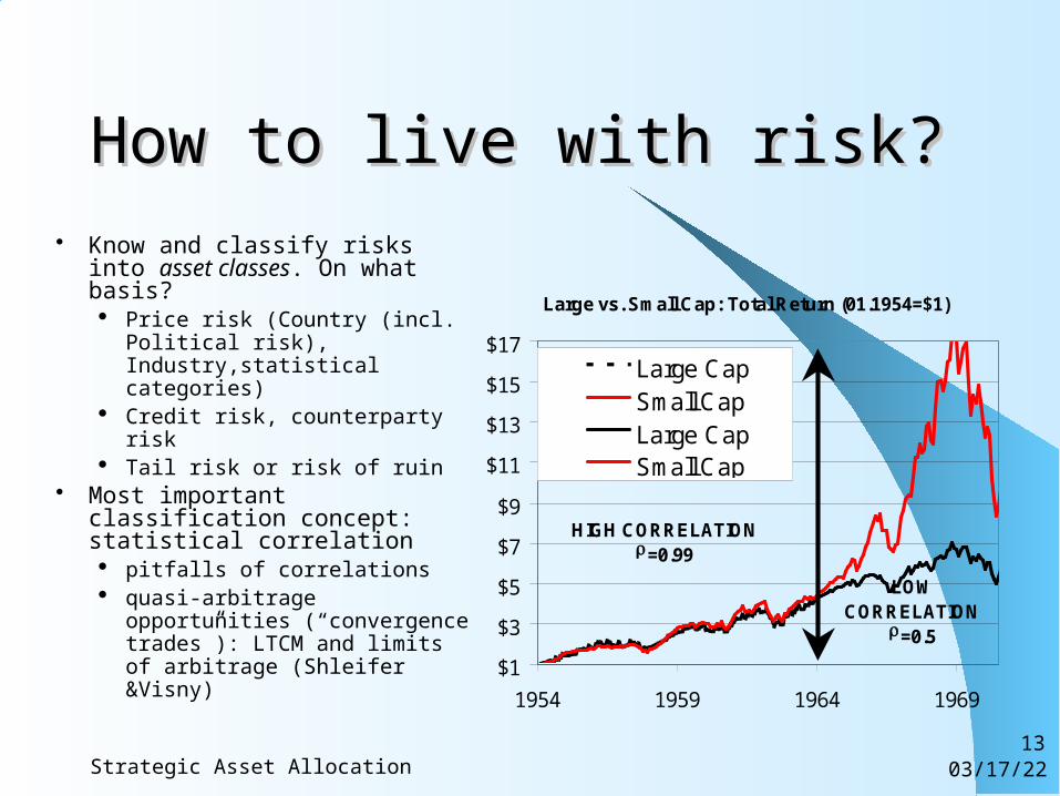
How to live with risk?How to live with risk? Know and classify risks into

asset classes. On what basis? Price risk (Country (incl.

Political risk), Industry,statistical categories)

Credit risk, counterparty risk Tail risk or risk of ruin

Most important classification concept: statistical correlation pitfalls of correlations quasi-arbitrage opportunities

(“convergence trades”): LTCM and limits of arbitrage (Shleifer &Visny)

Large vs. Small Cap: Total Return (01.1954=$1)

$1

$3

$5

$7

$9

$11

$13

$15

$17

1954 1959 1964 1969

Large CapSmall CapLarge CapSmall Cap

HIGH CORRELATIONr=0.99

LOW CORRELATION

r=0.5


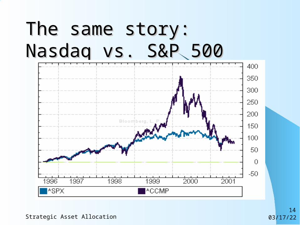
The same story:The same story: Nasdaq vs. S&P 500Nasdaq vs. S&P 500



Henry Lowenfeld, 1909Henry Lowenfeld, 1909

“It is significant to see how entirely all the rest of the Geographically Distributed stocks differ in their price movements from the British stock. It is this individuality of movement on the part of each security, included in a well-distributed Investment List, which ensures the first great essential of successful investment, namely, Capital Stability.”

From: Investment and Exact Science, 1909.


Globalization and Financial Globalization and Financial LinkagesLinkages Common wisdom is that globalization and

integration of markets accentuates financial linkages (correlations)– Business cycle synchronization– Policy coordination– Coordination of institutions– Decrease in “home bias” of investors– Globalization of firms

Globalization and integration also allows country specialization


What is the overall effect?What is the overall effect?

Decrease in expected returns Higher correlation between asset markets More markets for investment Increase in the types of marketed securities Potential synchronization of business cycles Increased policy coordination

Net effect?


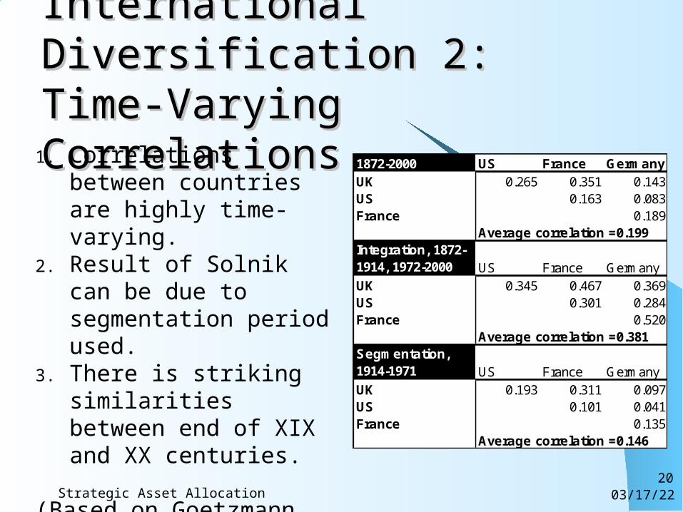
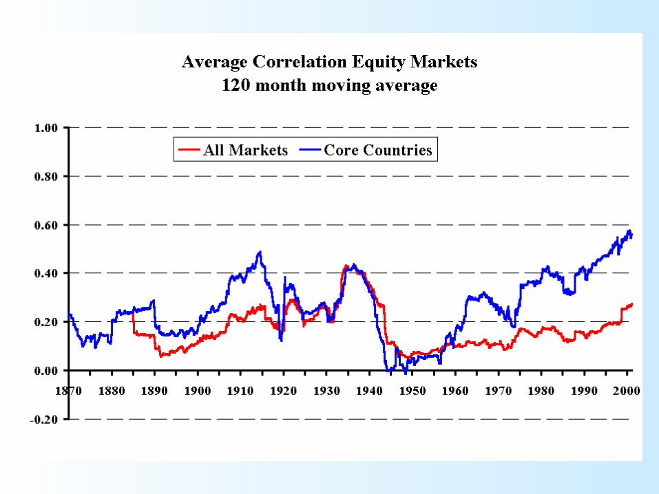
International Diversification 2: International Diversification 2: Time-Varying CorrelationsTime-Varying Correlations

1872-2000 US France GermanyUK 0.265 0.351 0.143US 0.163 0.083France 0.189

Average correlation =0.199Integration, 1872-1914, 1972-2000 US France GermanyUK 0.345 0.467 0.369US 0.301 0.284France 0.520

Average correlation =0.381Segmentation, 1914-1971 US France GermanyUK 0.193 0.311 0.097US 0.101 0.041France 0.135

Average correlation =0.146

1. Correlations between countries are highly time-varying.

2. Result of Solnik can be due to segmentation period used.

3. There is striking similarities between end of XIX and XX centuries.

(Based on Goetzmann et. al. NBER W8612)


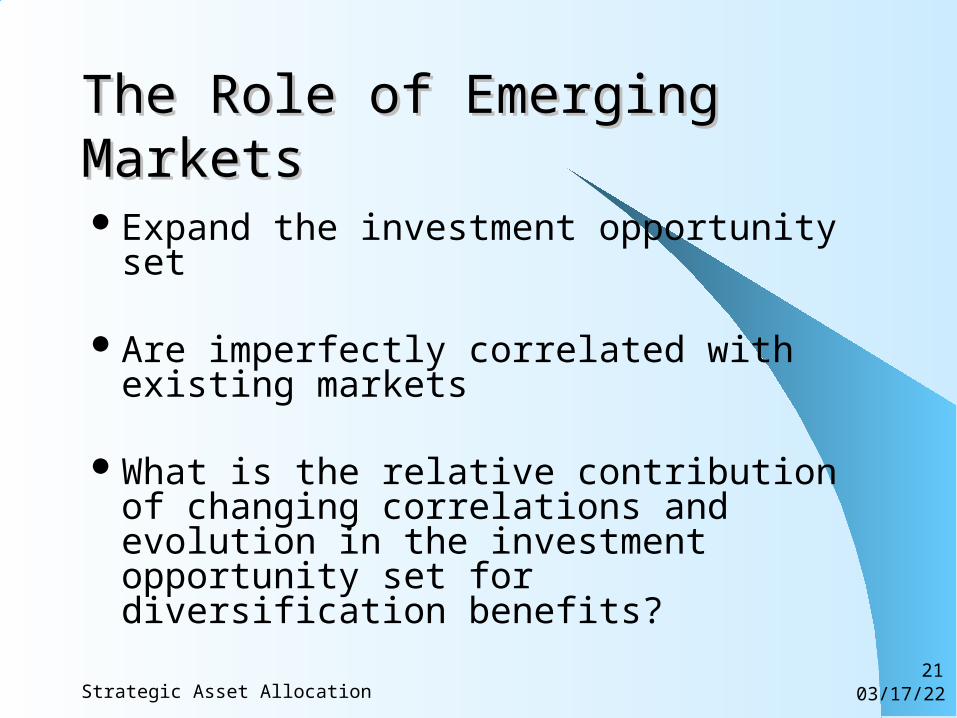
The Role of Emerging MarketsThe Role of Emerging Markets

Expand the investment opportunity set

Are imperfectly correlated with existing markets

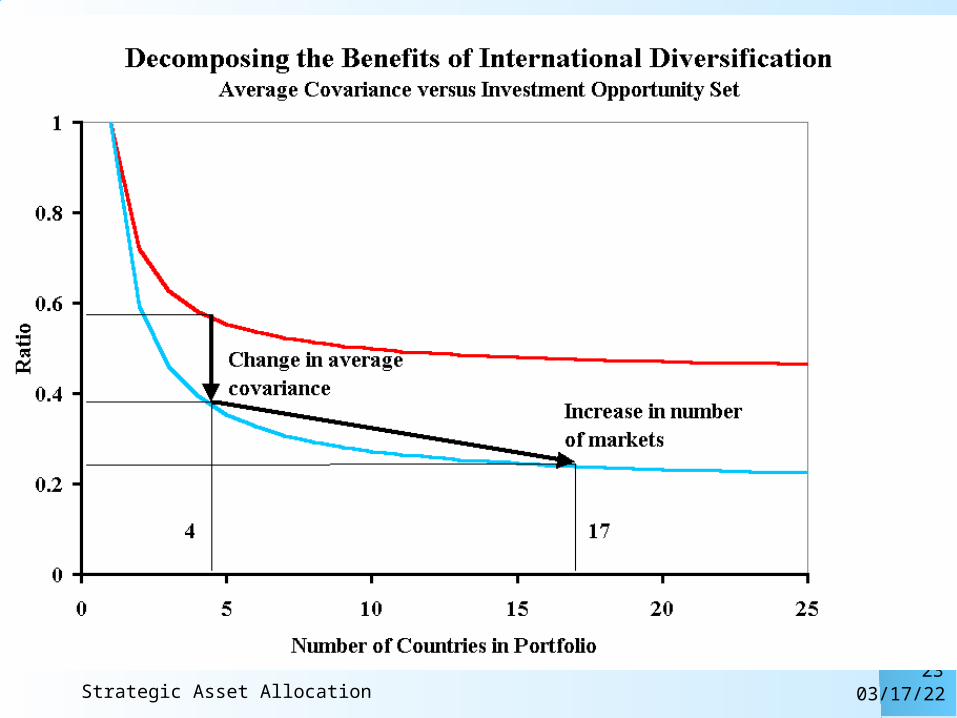
What is the relative contribution of changing correlations and evolution in the investment opportunity set for diversification benefits?


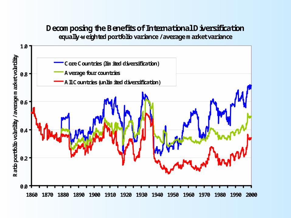
Decomposing the Benefits of International Diversificationequally-weighted portfolio variance / average market variance

0.0

0.2

0.4

0.6

0.8

1.0

1860 1870 1880 1890 1900 1910 1920 1930 1940 1950 1960 1970 1980 1990 2000

Rat

io p

ortf

olio

vol

atili

ty /

aver

age

mar

ket

vola

tilit

y

Core Countries (limited diversification)

Average four countries

All Countries (unlimited diversification)


Bottom Line: International Diversification Bottom Line: International Diversification Does Not Work as it Used to...Does Not Work as it Used to...

•Trade barriers disappear (NAFTA, EU, ASEAN, etc.)•Globalization of Business Enterprises,•Wave of intra-industry M&A (incl. cross-border M&A)

“…active portfolio managers will have increasing difficulty addingvalue by using a top-down strategy through European countryallocation.” (Freiman, 1998)

New Holy Graal: Industry Diversification


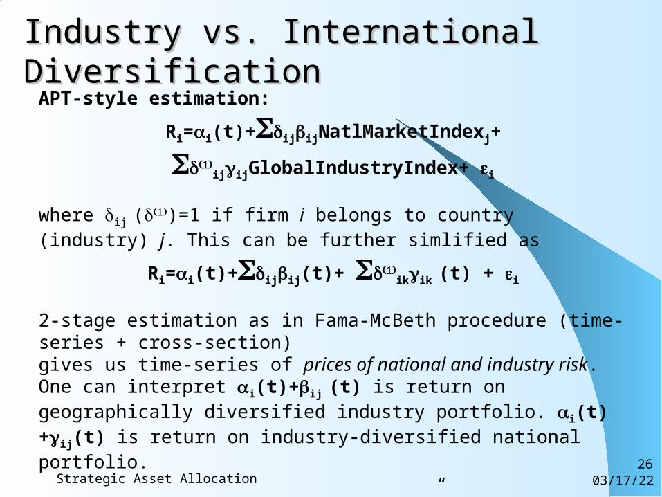
Industry vs. International DiversificationIndustry vs. International DiversificationAPT-style estimation:

Ri=i(t)+ijijNatlMarketIndexj+ ijijGlobalIndustryIndex+ i

where ij ()=1 if firm i belongs to country (industry) j. This can be further simlified as

Ri=i(t)+ijij(t)+ ikik (t) + i

2-stage estimation as in Fama-McBeth procedure (time-series + cross-section)gives us time-series of prices of national and industry risk. One can interpret i(t)+ij (t) is return on geographically diversified industry portfolio. i(t)+ij(t) is return on industry-diversified national portfolio.

Small Print: (a) We miss all “other” firm characteristics-size, b/m, dividend payout ratio, leverage, etc. (b)We also assume that securities in country i have same exposure to domestic and foreign factors. (c) We do not address Ericsson problem. (d) Cavaglia et. al. (2001) consider 35 industries in 21 countries.


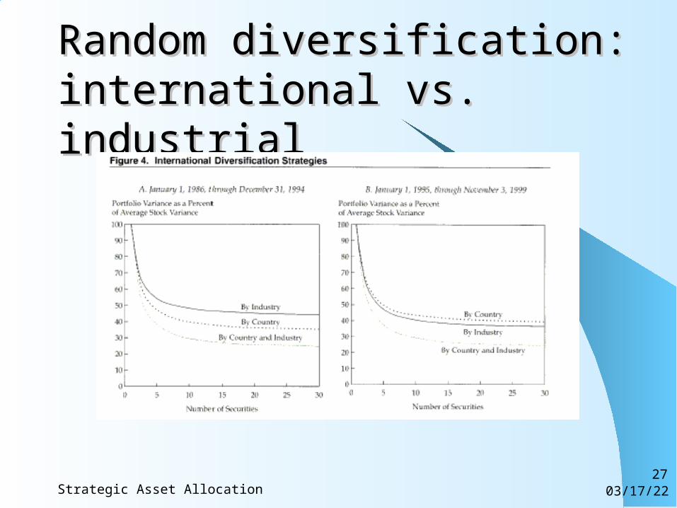
Random diversification: Random diversification: international vs. industrialinternational vs. industrial

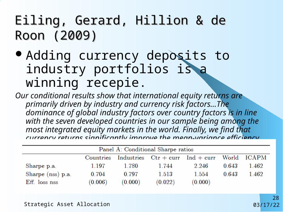
Eiling, Gerard, Hillion & de Roon (2009)Eiling, Gerard, Hillion & de Roon (2009)

Adding currency deposits to industry portfolios is a winning recepie.

Our conditional results show that international equity returns are primarily driven by industry and currency risk factors…The dominance of global industry factors over country factors is in line with the seven developed countries in our sample being among the most integrated equity markets in the world. Finally, we find that currency returns significantly improve the mean-variance efficiency of country, industry and world market portfolio returns.


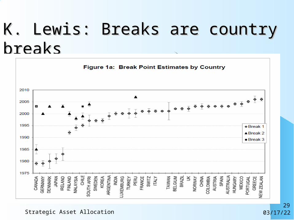
K. Lewis: Breaks are country breaksK. Lewis: Breaks are country breaks


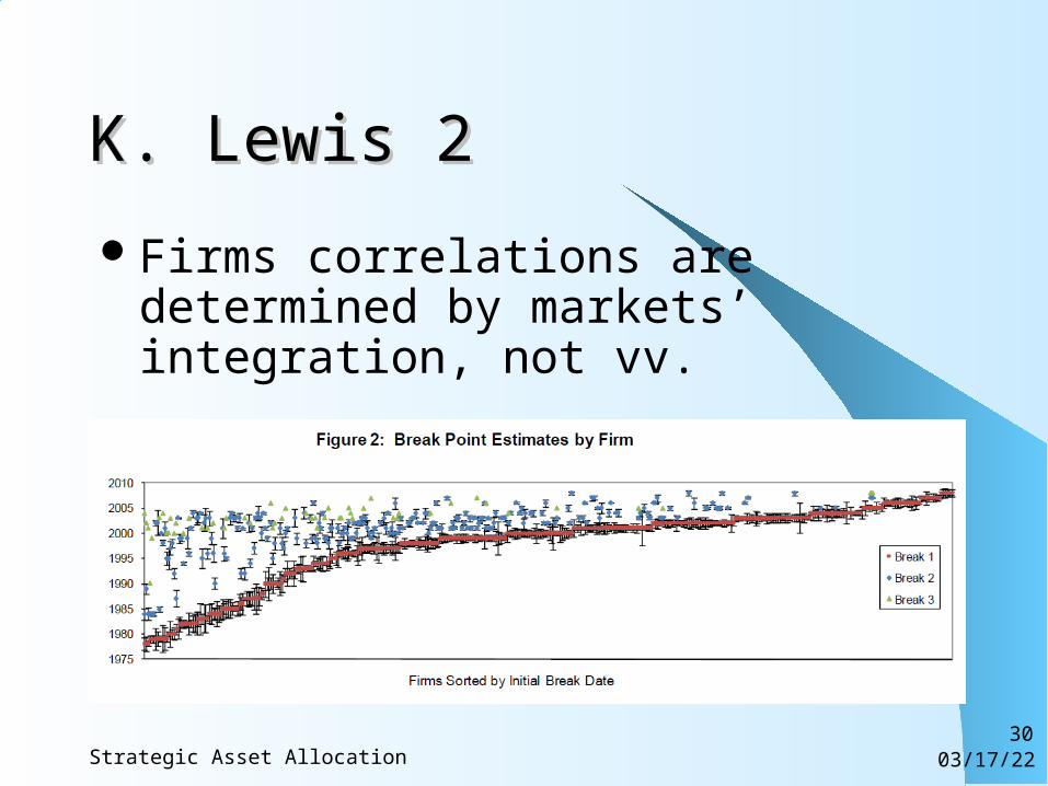
K. Lewis 2K. Lewis 2

Firms correlations are determined by markets’ integration, not vv.



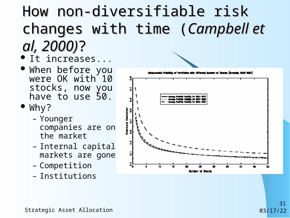
How non-diversifiable risk changes How non-diversifiable risk changes with time (with time (CampbellCampbell et al et al, , 2000)2000)?? It increases... When before you

were OK with 10 stocks, now you have to use 50.

Why?– Younger

companies are on the market

– Internal capital markets are gone

– Competition– Institutions


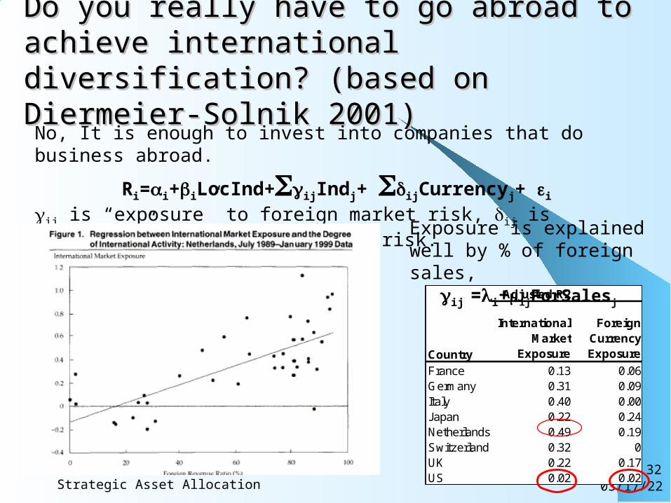
Do you really have to go abroad to achieve Do you really have to go abroad to achieve international diversification? (based on international diversification? (based on Diermeier-Solnik 2001)Diermeier-Solnik 2001)

No, It is enough to invest into companies that do business abroad.

Ri=i+iLocInd+ijIndj+ ijCurrencyj+ i

ij is “exposure” to foreign market risk, ij is “exposure” to foreign currency risk.

Adjusted R2

Country

International Market

Exposure

Foreign Currency Exposure

France 0.13 0.06Germany 0.31 0.09Italy 0.40 0.00Japan 0.22 0.24Netherlands 0.49 0.19Switzerland 0.32 0UK 0.22 0.17US 0.02 0.02

Exposure is explained well by % of foreign sales,

ij =i+ijForSalesj


Word of caution:Word of caution:

“Trust companies…have reckoned that by a wide spreading of their investment risk, a stable revenue position could be maintained, as it was not to be expected that all the world would go wrong at the same time. But the unexpected has happened, and every part of the civilized world is in trouble…”

Chairman of Alliance Trust Company (1929)



Non traded riskNon traded riskss Human capital and death insurance Investment in residence Other consumption needs: saving for

retirement and life insurance Liabilities: B/S optimization You must consider that these are part and

parcel of your portfolio, but with immutable weights


Human CapitalHuman Capital Most of the ”normal” individual wealth is in the form

of HUMAN CAPITAL. Assume that human capital supply (willingness to

work) is flexible and tradeable. Value of future cash flow decreases with time.

Share of stocks will go down with time The higher is the riskiness of human capital, the less is

the willingness to invest in stock Strong effect on portfolio decisions. Real estate can amplify riskiness of human capital


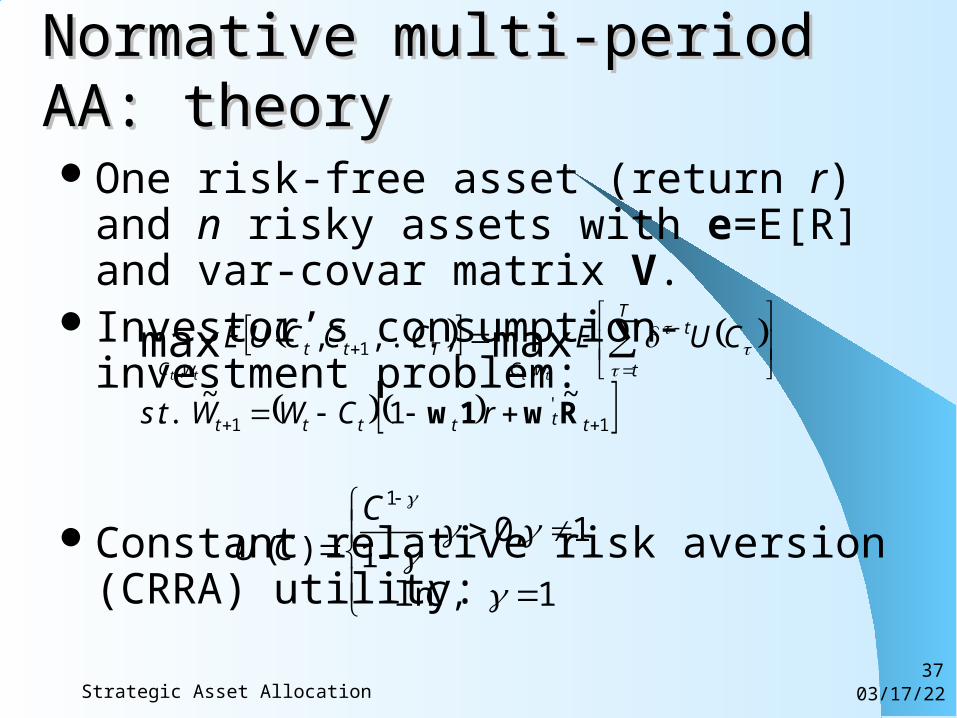
Normative multi-period AA: theoryNormative multi-period AA: theory

One risk-free asset (return r) and n risky assets with e=E[R] and var-covar matrix V.

Investor’s consumption-investment problem:

Constant relative risk aversion (CRRA) utility:

1'

1

,1

,

~1

~ ..

,...,, maxmax

tttttt

T

t

t

wCTtt

wC

rCWWts

CUECCCUEtttt

Rw1w

1 ,ln

1,0 ,1)(

1

C

CCU


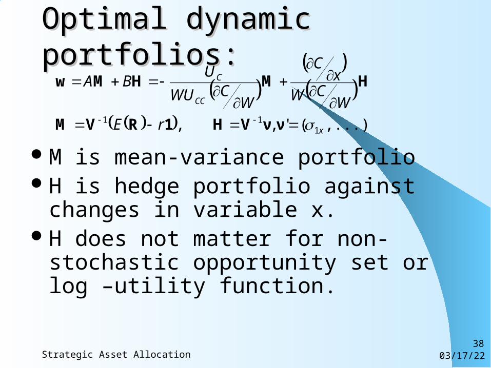
Optimal dynamic portfolios:Optimal dynamic portfolios:

M is mean-variance portfolio H is hedge portfolio against changes in

variable x. H does not matter for non-stochastic

opportunity set or log –utility function.

,...)(', , 111

x

CC

C

rE

WCW

xC

WCWU

UBA

ννVH1RVM

HMHMw


ConstraintsConstraints Liquidity Regulations: public or self imposed

SEC Pension funds: Employee Retirement Income Security Act

(ERISA); European directives no more than 5% in any publicly traded company Mostly domestic assets

Mutual funds: No borrowing. Association for Investment Management and Research (AIMR)

Taxes Unique needs: internal restrictions


Standard Deviation (Risk)

Expected Return

0.0 42.03.0 6.0 9.0 12.0 15.0 18.0 21.0 24.0 27.0 30.0 33.0 36.0 39.02.0

19.0

3.0

4.0

5.0

6.0

7.0

8.0

9.0

10.0

11.0

12.0

13.0

14.0

15.0

16.0

17.0

18.0

S&P500

IA Small Stocks

Russell 2000

MSCI Europe

MSCI Pacific TR

IA Corporate

IA 20Yr GvtIA 5YR Gvt

IA 1 Year GvtNon-US LT Gvt

30 Day TBILL

Gold

CRSP MidCap

Real Estate

S&P500 (20.0%)

IA Small Stocks (7.5%)MSCI Europe (19.7%)

MSCI Pacific TR (7.5%)

IA 5YR Gvt (4.5%)

IA 1 Year Gvt (20.0%)

Real Estate (20.0%)

S&P500 (51.8%)

IA Small Stocks (2.6%)

MSCI Europe (11.9%)

MSCI Pacific TR (10.2%)Real Estate (23.5%)

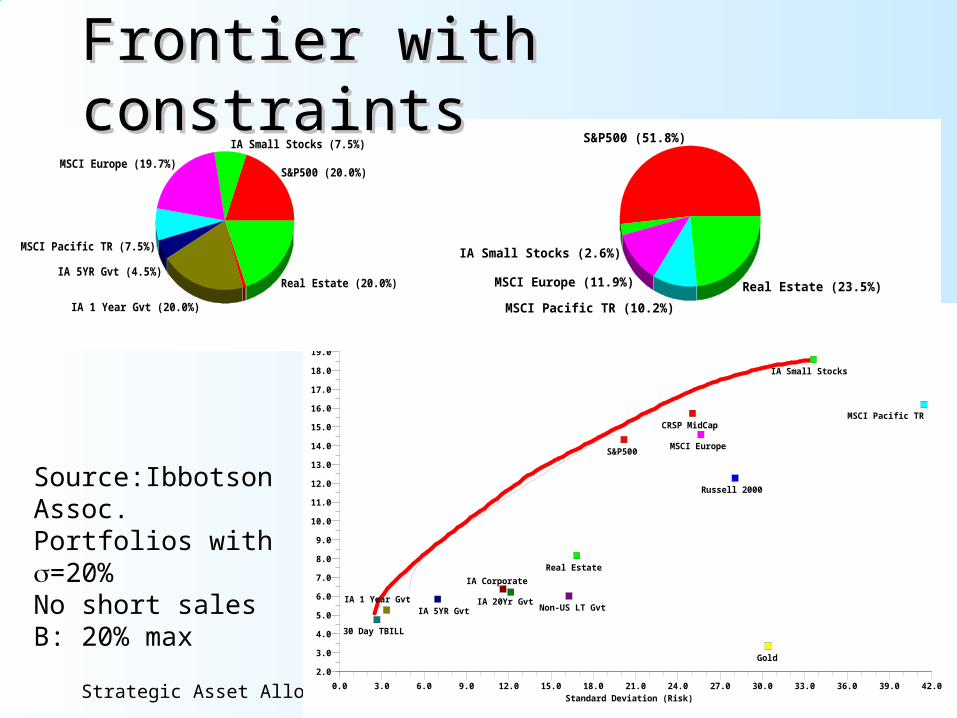
Frontier with constraintsFrontier with constraints

Source:Ibbotson Assoc.Portfolios with =20%No short salesB: 20% max


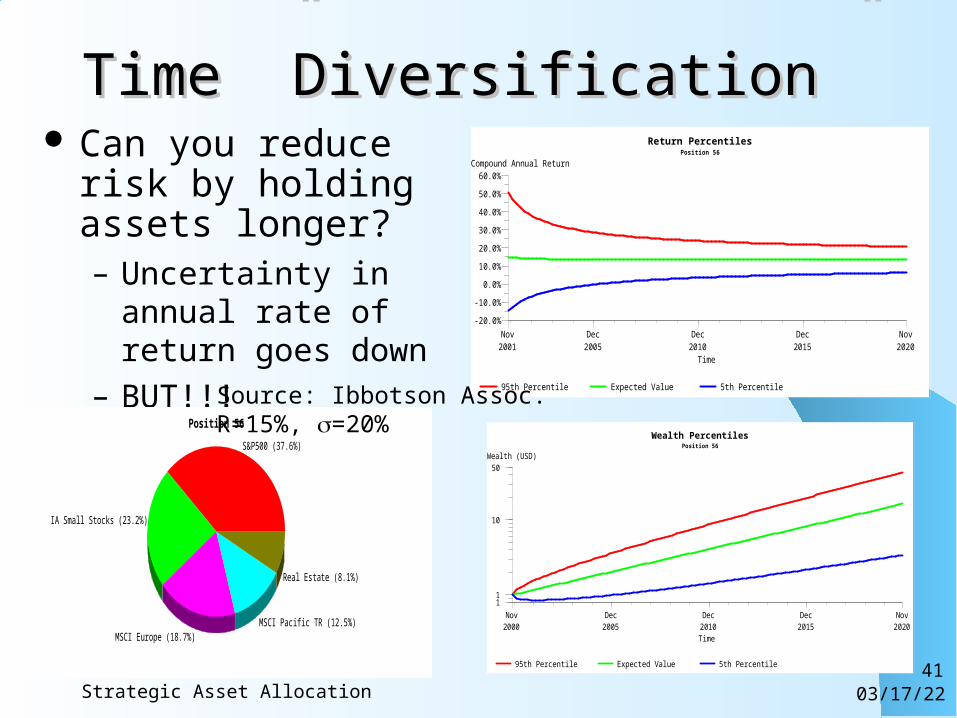
Time ”Diversification”Time ”Diversification” Can you reduce risk by

holding assets longer?– Uncertainty in annual

rate of return goes down

– BUT!!! Uncertainty of total returns goes up

Position 56

S&P500 (37.6%)

IA Small Stocks (23.2%)

MSCI Europe (18.7%)MSCI Pacific TR (12.5%)

Real Estate (8.1%)

Time

Compound Annual ReturnPosition 56

Return Percentiles

Nov2001

Nov2020

Dec2005

Dec2010

Dec2015

-20.0%

60.0%

-10.0%

0.0%

10.0%

20.0%

30.0%

40.0%

50.0%

95th Percentile Expected Value 5th Percentile

Time

Wealth (USD)Position 56

Wealth Percentiles

Nov2000

Nov2020

Dec2005

Dec2010

Dec2015

1

50

1

10

95th Percentile Expected Value 5th Percentile

Source: Ibbotson Assoc.R=15%, =20%


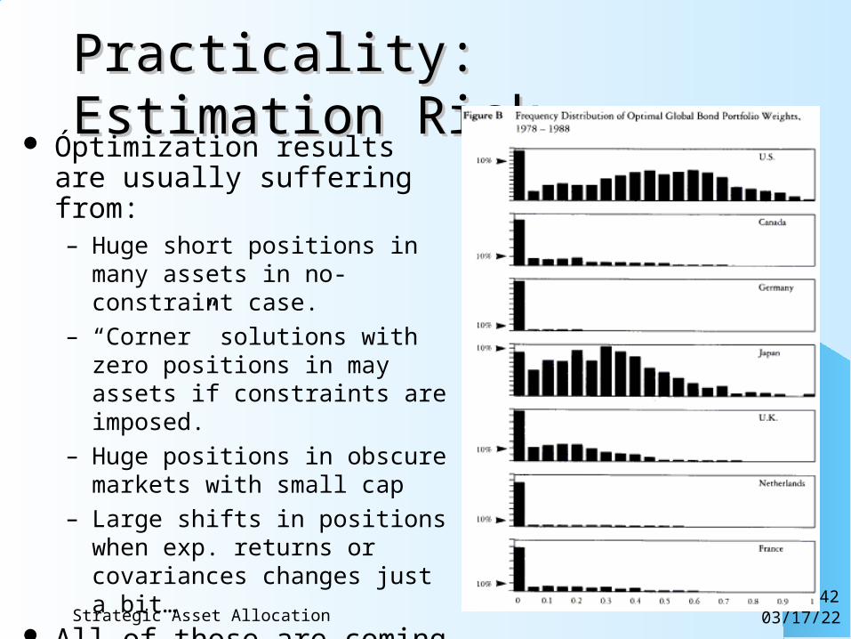
Practicality: Estimation RiskPracticality: Estimation Risk Óptimization results are usually

suffering from:– Huge short positions in many assets in

no-constraint case.

– “Corner” solutions with zero positions in may assets if constraints are imposed.

– Huge positions in obscure markets with small cap

– Large shifts in positions when exp. returns or covariances changes just a bit…

All of those are coming from one common cause: difficulties in estimation of expected returnsexpected returns.

04/18/23Asset Pricing Models43

Another example (GS 2003):Another example (GS 2003):

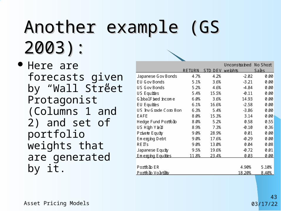
Here are forecasts given by “Wall Street Protagonist” (Columns 1 and 2) and set of portfolio weights that are generated by it.

RETURN STD DEVUnconstrained weights

No Short Sales

Japanese Gov Bonds 4.7% 4.2% -2.02 0.00EU Gov Bonds 5.1% 3.6% -3.21 0.00US Gov Bonds 5.2% 4.6% -4.84 0.00US Equities 5.4% 15.5% -0.11 0.00Global Fixed income 6.0% 3.6% 14.93 0.00EU Equities 6.1% 16.6% -2.58 0.00US Inv Grade Corp Bonds 6.3% 5.4% -3.86 0.00EAFE 8.0% 15.3% 3.14 0.00Hedge Fund Portfolio 8.0% 5.2% 0.58 0.55US High Yield 8.9% 7.3% -0.10 0.36Private Equity 9.0% 28.9% 0.01 0.00Emerging Debt 9.0% 17.6% -0.29 0.00REITs 9.0% 13.0% 0.04 0.08Japanese Equity 9.5% 19.6% -0.72 0.01Emerging Equities 11.8% 23.4% 0.03 0.00

Portfolio ER 4.90% 5.10%Portfolio Volatility 18.20% 8.40%


Equilibrium and individual Equilibrium and individual asset’ expected returnasset’ expected returnOne can expect that ERP is between 4 and

6% and is fairly stable with time (see later in the course)

One can make forecast for individual assets that are different from long term premium.

But by forecasting one asset class, we are implicitly making forecast for other asset classes as well.


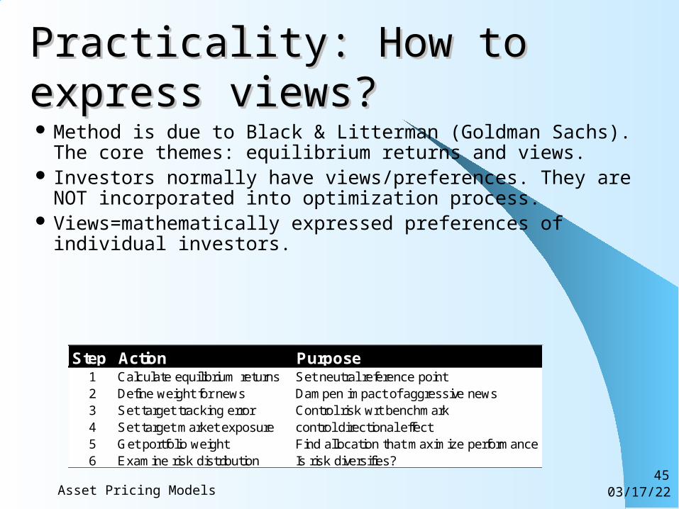
Practicality: How to express Practicality: How to express views?views? Method is due to Black & Litterman (Goldman Sachs). The core

themes: equilibrium returns and views. Investors normally have views/preferences. They are NOT

incorporated into optimization process. Views=mathematically expressed preferences of individual

investors.

Step Action Purpose1 Calculate equilibrium returns Set neutral reference point2 Define weight for news Dampen impact of aggressive news3 Set target tracking error Control risk wrt benchmark4 Set target market exposure control directional effect5 Get portfolio weight Find allocation that maximize performance6 Examine risk distribution Is risk diversifies?


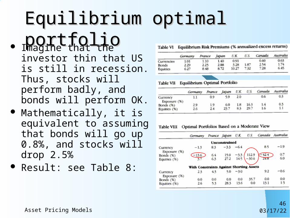
Equilibrium optimal portfolioEquilibrium optimal portfolio Imagine that the investor thin

that US is still in recession. Thus, stocks will perform badly, and bonds will perform OK.

Mathematically, it is equivalent to assuming that bonds will go up 0.8%, and stocks will drop 2.5%

Result: see Table 8:


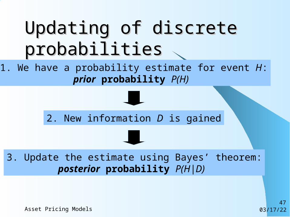
Updating of discrete Updating of discrete probabilitiesprobabilities

1. We have a probability estimate for event H:prior probability P(H)

2. New information D is gained

3. Update the estimate using Bayes’ theorem:posterior probability P(H|D)


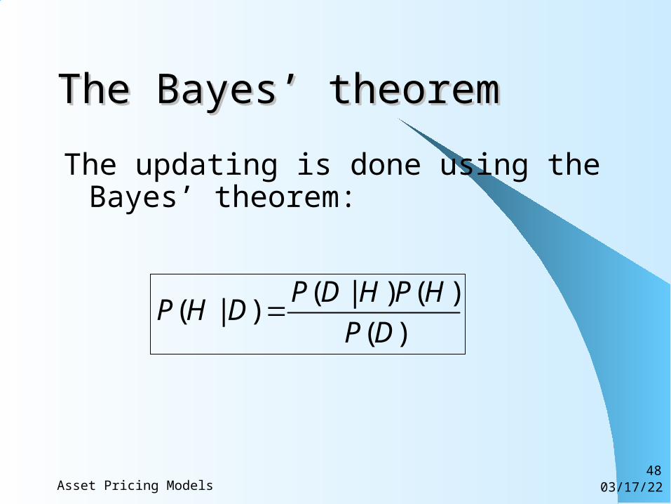
The Bayes’ theoremThe Bayes’ theorem

The updating is done using the Bayes’ theorem:

( | ) ( )( | )

( )

P D H P HP H D

P D


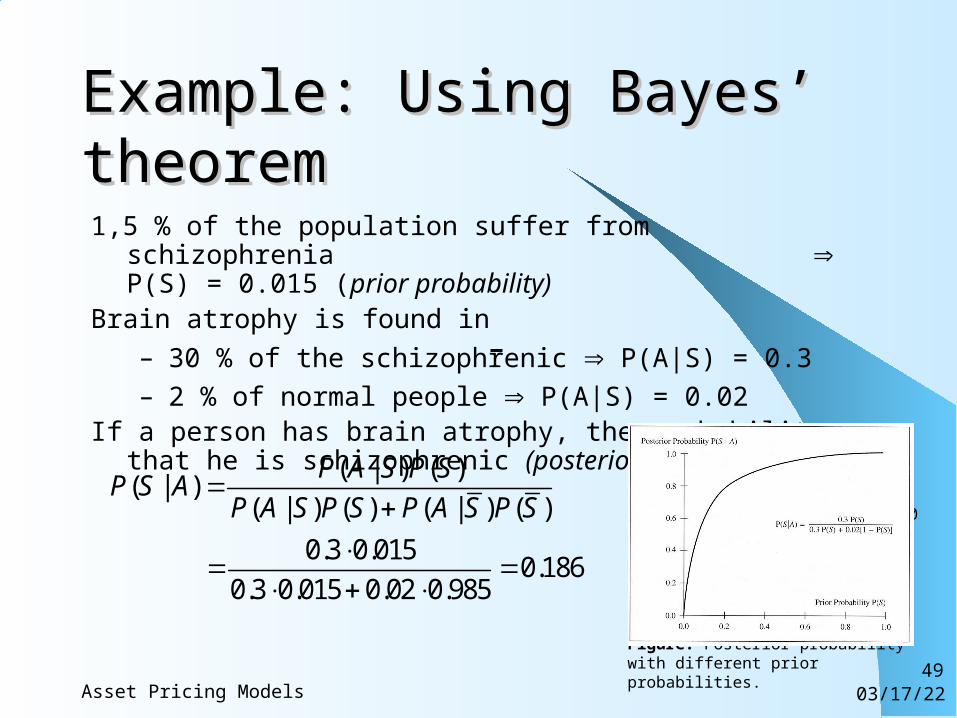
Example: Using Bayes’ Example: Using Bayes’ theoremtheorem1,5 % of the population suffer from schizophrenia

P(S) = 0.015 (prior probability)Brain atrophy is found in

– 30 % of the schizophrenic P(A|S) = 0.3

– 2 % of normal people P(A|S) = 0.02If a person has brain atrophy, the probability that he is schizophrenic

(posterior probability) is:

( | ) ( )( | )

( | ) ( ) ( | ) ( )

0.3 0.0150.186

0.3 0.015 0.02 0.985

P A S P SP S A

P A S P S P A S P S

Picture: Clemen s. 250

Figure: Posterior probability with different prior probabilities.


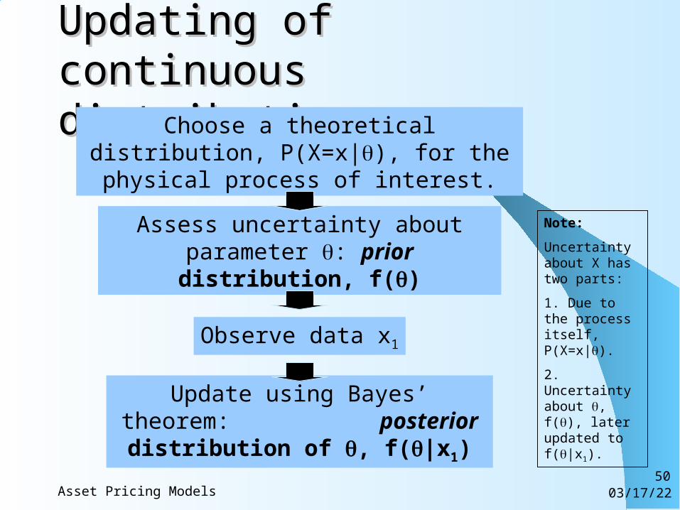
Updating of continuous Updating of continuous distributionsdistributions

Choose a theoretical distribution, P(X=x|), for the physical process of interest.

Assess uncertainty about parameter : prior distribution, f()

Observe data x1

Update using Bayes’ theorem: posterior distribution of , f(|x1)

Note:

Uncertainty about X has two parts:

1. Due to the process itself, P(X=x|).

2. Uncertainty about , f(), later updated to f(|x1).


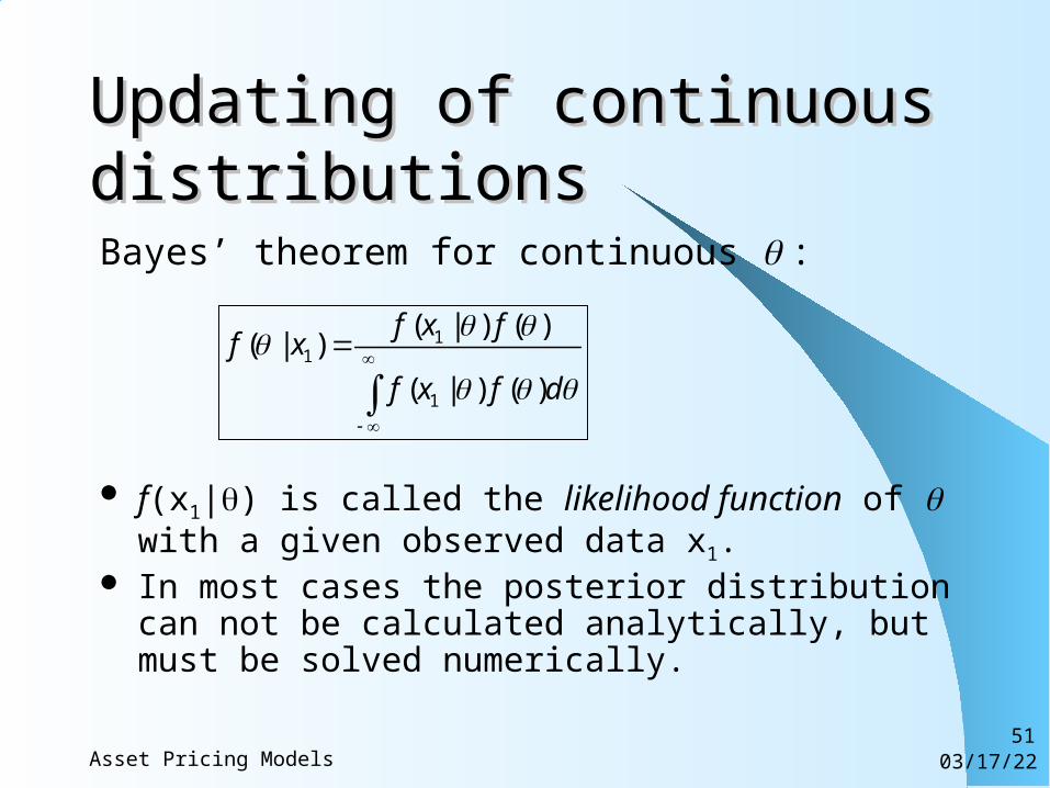
Updating of continuous Updating of continuous distributionsdistributionsBayes’ theorem for continuous :

f(x1|) is called the likelihood function of with a given observed data x1.

In most cases the posterior distribution can not be calculated analytically, but must be solved numerically.

11

1

( | ) ( )( | )

( | ) ( )

f x ff x

f x f d


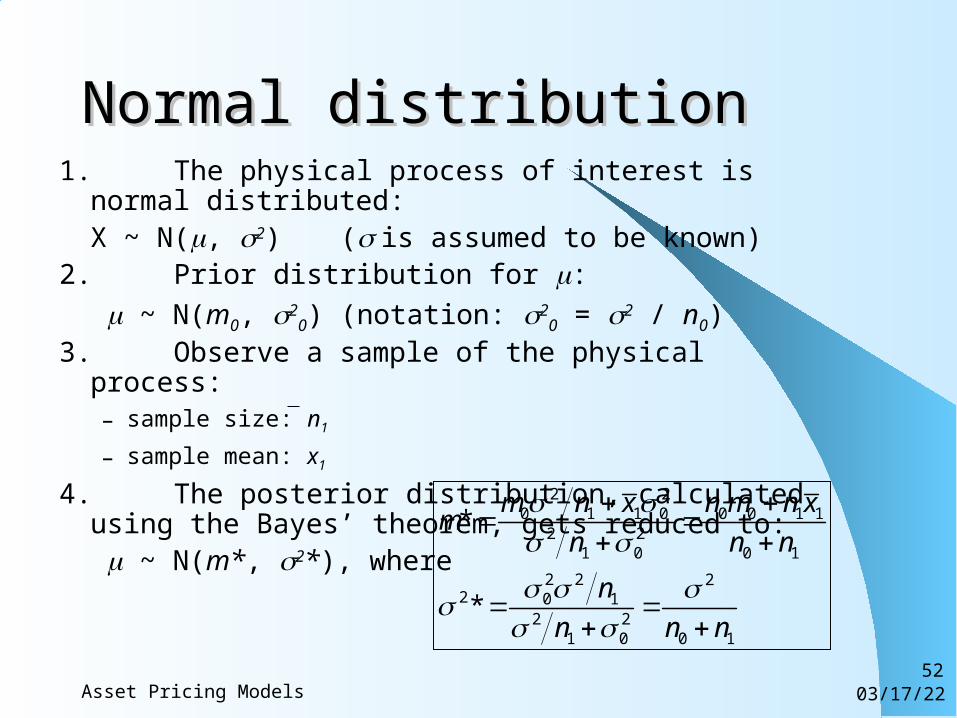
Normal distributionNormal distribution1. The physical process of interest is normal distributed:

X ~ N(, 2) ( is assumed to be known)2. Prior distribution for :

~ N(m0, 20)(notation: 2

0 = 2 / n0)3. Observe a sample of the physical process:

– sample size: n1

– sample mean: x1

4. The posterior distribution, calculated using the Bayes’ theorem, gets reduced to: ~ N(m*, 2*), where

2 20 1 1 0 0 0 1 1

2 21 0 0 1

2 2 22 0 1

2 21 0 0 1

*

*

m n x n m n xm

n n n

n

n n n


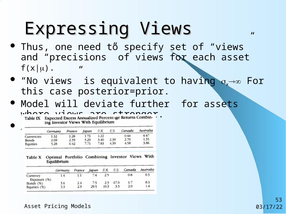
Expressing ViewsExpressing Views Thus, one need to specify set of “views” and “precisions” of

views for each asset f(x|). “No views” is equivalent to having x For this case

posterior=prior. Model will deviate further for assets where views are stronger. All assets are affected:


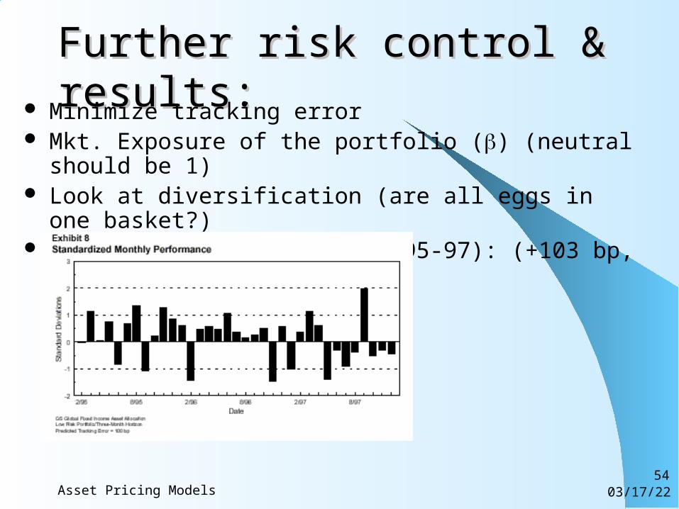
Further risk control & results:Further risk control & results: Minimize tracking error Mkt. Exposure of the portfolio () (neutral should be 1) Look at diversification (are all eggs in one basket?) Results (according to GS, 95-97): (+103 bp, +83 bp, -26bp)


Other uses:Other uses:

Black-Litterman model is essentially Tactical Asset Allocation model (provided that algorithm of selecting “views” is specified).

But it can be used effectively in updating priors on the distribution of the signals.

It can be used to bring in new asset classes for which the recorded history is short or unreliable (venture capital funds, hedge funds, emerging markets, etc.)


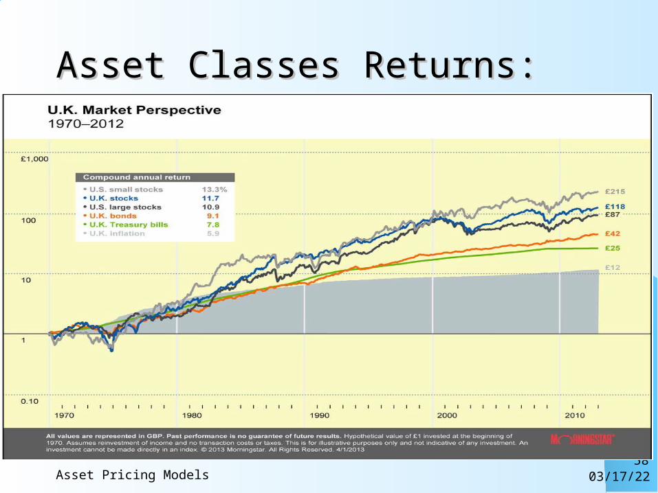
What is expected risk premium?What is expected risk premium?

Expected risk premium= Var(rM)/E[W/]Plays central role in any discussion about

the marketWhat is that? How to measure it? What

will it tell us about mankind and economy (or Asset Pricing Model)?– Historical perspective– Equilibrium perspective


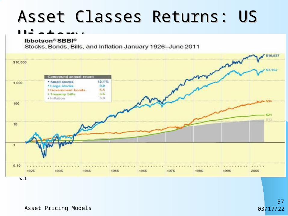
Asset Classes Returns: US HistoryAsset Classes Returns: US History

0.1

1

10

100

1000

10000

Jan1926

Jan1931

Jan1936

Jan1941

Jan1946

Jan1951

Jan1956

Jan1961

Jan1966

Jan1971

Jan1976

Jan1981

Jan1986

Jan1991

Jan1996

Jan2001

U.S. LT Gvt TR

U.S. 30 Day TBill TR

S&P 500 TR

U.S. Inflation

U.S. Small Stk TR


Asset Classes Returns: Swedish Asset Classes Returns: Swedish HistoryHistory

0.1

1

10

100

1000

10000

100000

1000000

1900 1920 1940 1960 1980 2000

1 S

EK

inve

sted

in 1

900

DMS Global Sweden Bill TR

DMS Global Sweden Inflation

DMS Global Sweden Equity TR

DMS Global Sweden Bond TR


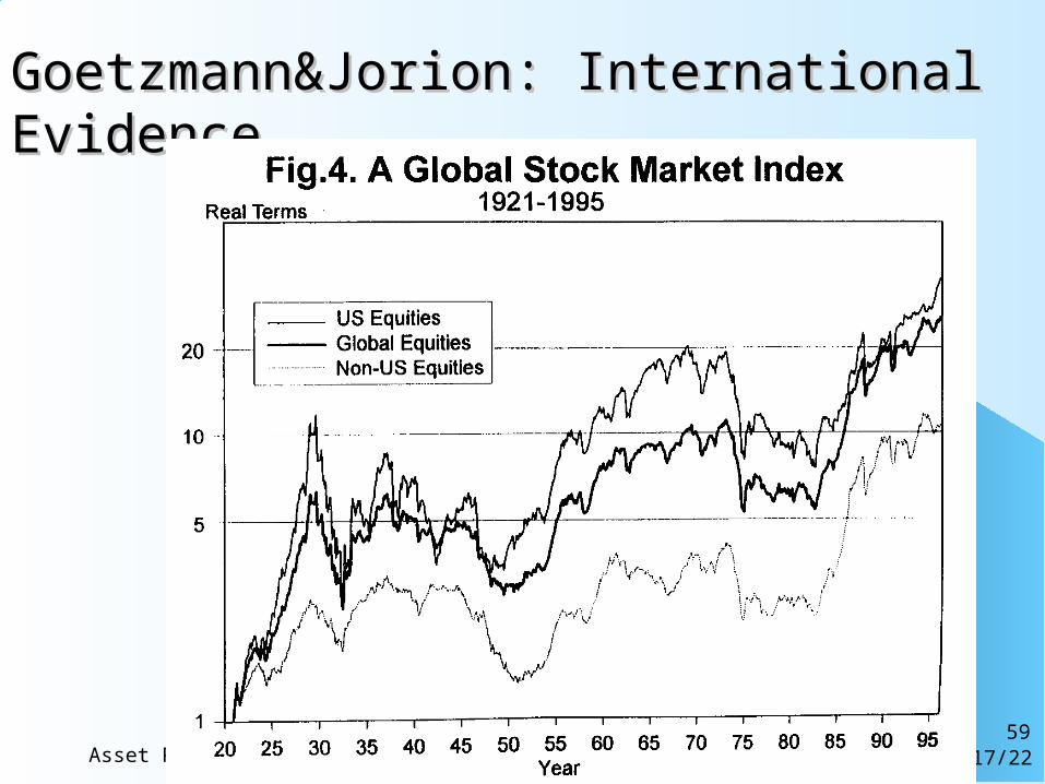
Goetzmann&Jorion: International EvidenceGoetzmann&Jorion: International Evidence


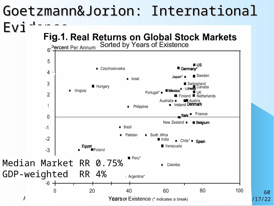
Goetzmann&Jorion: International EvidenceGoetzmann&Jorion: International Evidence

Median Market RR 0.75%GDP-weighted RR 4%


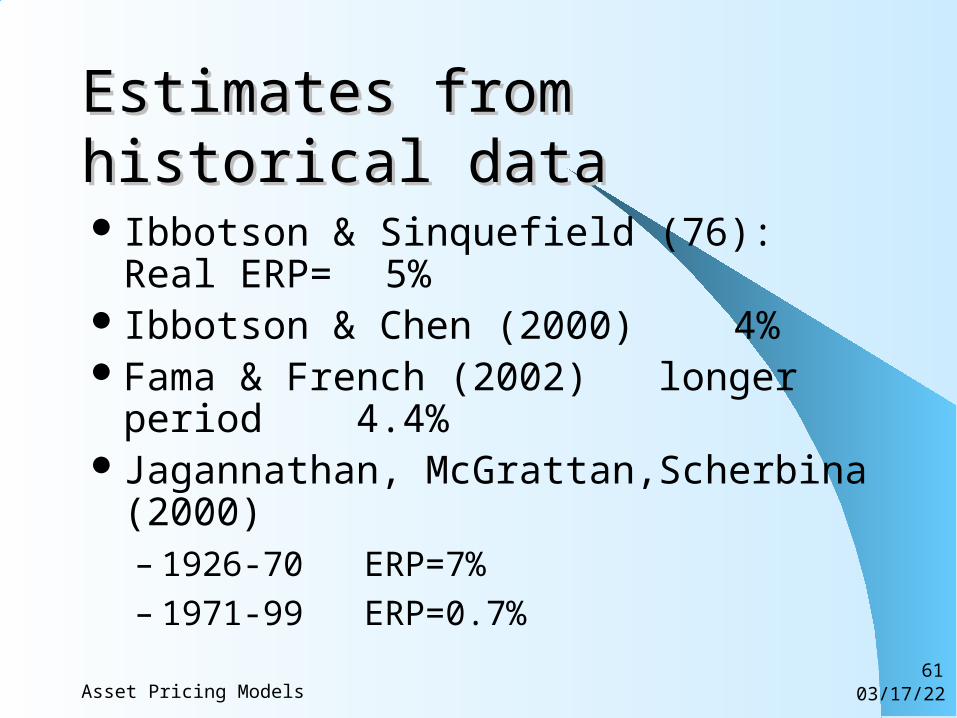
Estimates from historical dataEstimates from historical data

Ibbotson & Sinquefield (76): Real ERP=5%

Ibbotson & Chen (2000) 4%

Fama & French (2002) longer period 4.4%Jagannathan, McGrattan,Scherbina (2000)

– 1926-70 ERP=7%– 1971-99 ERP=0.7%

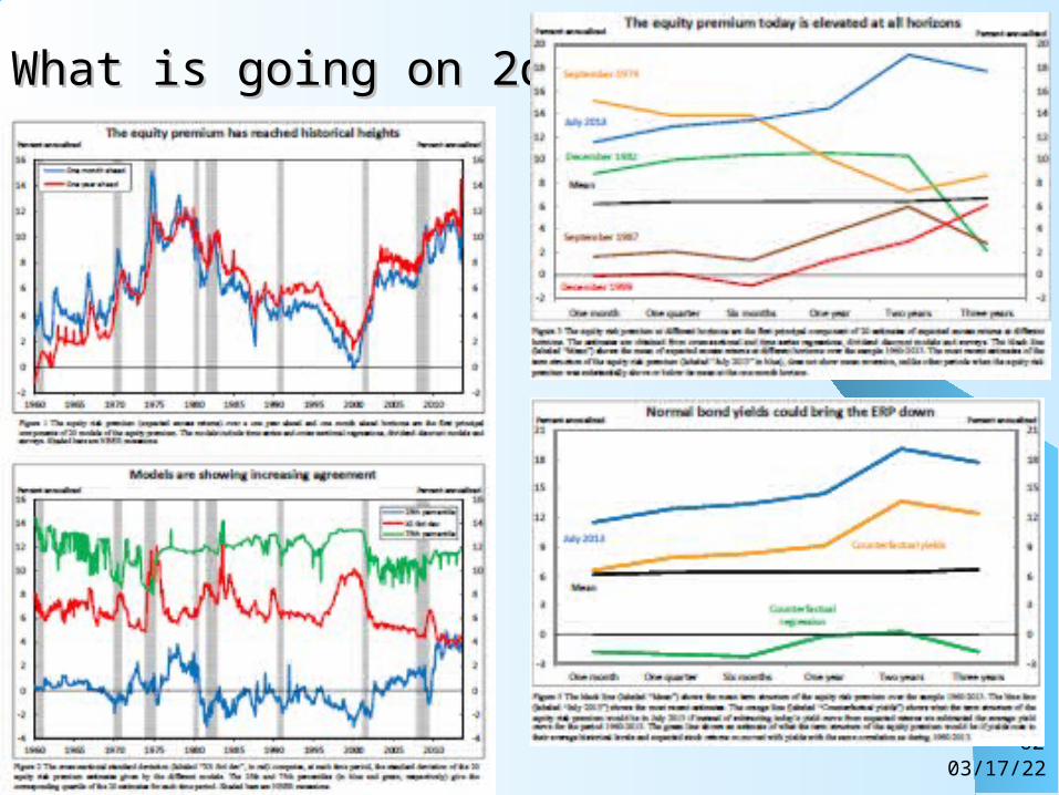
What is going on 2day?What is going on 2day?



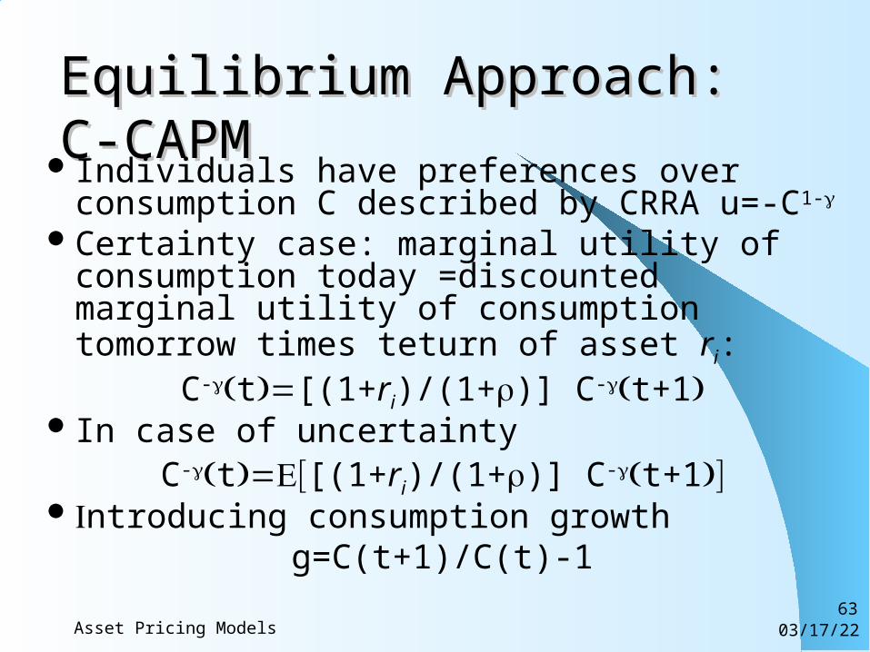
Equilibrium Approach: C-CAPMEquilibrium Approach: C-CAPMIndividuals have preferences over consumption

C described by CRRA u=-C1-

Certainty case: marginal utility of consumption today =discounted marginal utility of consumption tomorrow times teturn of asset ri:

C-t[(1+ri)/(1+r)] C-t+1In case of uncertainty

C-t[(1+ri)/(1+r)] C-t+1ntroducing consumption growth

g=C(t+1)/C(t)-1


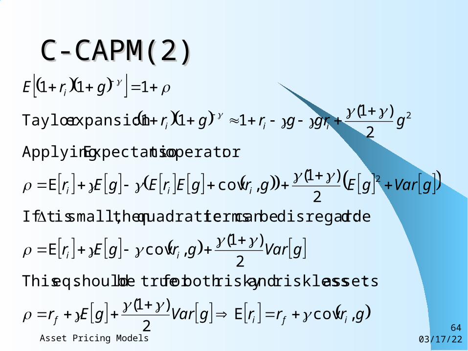
C-CAPM(2)C-CAPM(2)

grrrgVargEr

gVargrgEr

gVargEgrgErEgEr

ggrgrgr

grE

ifif

ii

iii

iii

i

,covE2

)1(

:assets riskless andrisky both for truebe should eq. This2

)1(,covE

:ddisregarde becan termsquadratic then small, ist If2

)1(,covE

:operator nsExpectatio Applying2

)1(111 :expansionTaylor

111

2

2

r

r

r

r


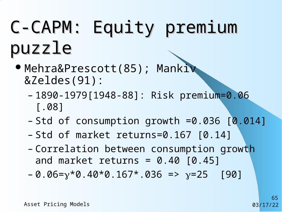
C-CAPM: Equity premium puzzleC-CAPM: Equity premium puzzle

Mehra&Prescott(85); Mankiv &Zeldes(91):– 1890-1979[1948-88]: Risk premium=0.06 [.08]– Std of consumption growth =0.036 [0.014]– Std of market returns=0.167 [0.14]– Correlation between consumption growth and

market returns = 0.40 [0.45]– 0.06=*0.40*0.167*.036 => =25 [90]


Equity premium puzzleEquity premium puzzle

Gamble: take 20% paycut if state of the world is ”bad” (prob=1/2) and stay at your current salary in good state, or agree on permanent cut of X%:

0.5*(0.8+1)=x


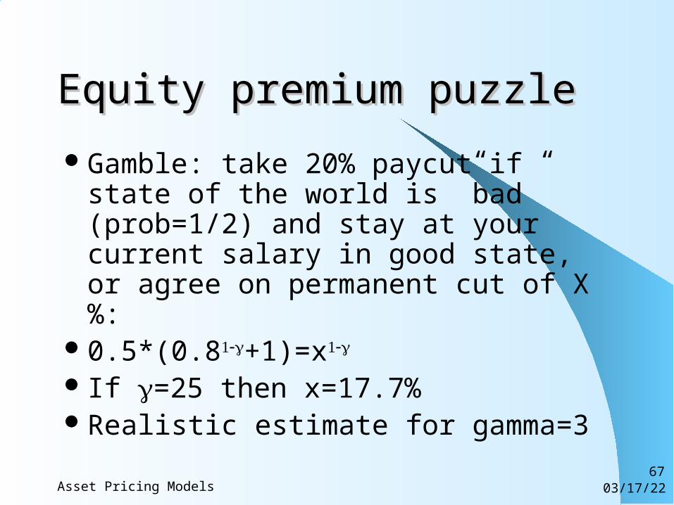
Equity premium puzzleEquity premium puzzle

Gamble: take 20% paycut if state of the world is ”bad” (prob=1/2) and stay at your current salary in good state, or agree on permanent cut of X%:

0.5*(0.8+1)=x

If =25 then x=17.7%Realistic estimate for gamma=3


How can we solve it? How can we solve it?

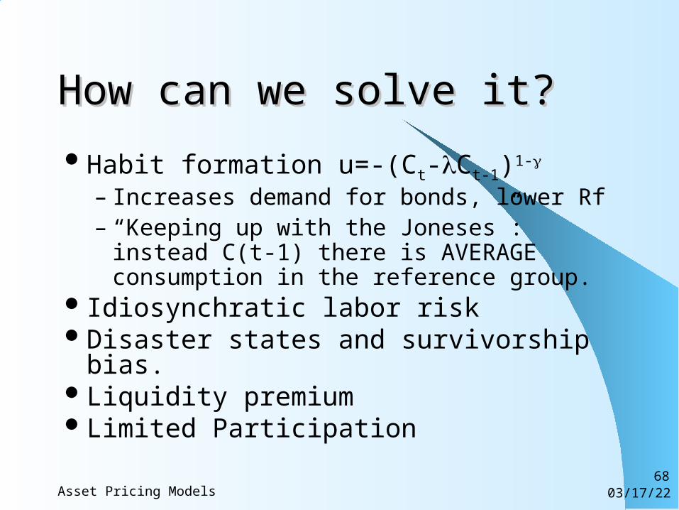
Habit formation u=-(Ct-Ct-1)1-

– Increases demand for bonds, lower Rf– “Keeping up with the Joneses”: instead C(t-1)

there is AVERAGE consumption in the reference group.

Idiosynchratic labor riskDisaster states and survivorship bias.Liquidity premiumLimited Participation

Documents

6/9/2015 Strategic Asset Allocation 1 Strategic Asset Allocation session 1 Andrei Simonov