Embed Size (px)
Citation preview
65-6514
FASSBERG, Harold Edward, 1919- CONTRIBUTIONS TO A CAPITAL MODEL WITH EFFICIENT PATHS OF CAPITAL ACCUMULATION BY USE OF THE CALCULUS OF VARIATIONS.
The American University, Ph. D ., 1965 Economics, theory
University Microfilms, Inc., Ann Arbor, Michigan
CONTRIBUTIONS TO A CAPITAL MODEL WITH EFFICIENT PATHS OF
CAPITAL ACCUMULATION BY USE OF THE CALCULUS OF VARIATIONS
A Dissertation
Presented to
the Faculty of the Graduate School
The American University
In Partial Fulfillment
of the Requirements for the Degree
Doctor of Philosophy
in Economics
byHarold E,-' Fassberg
December 1964
CONTRIBUTIONS TO A CAPITAL MODEL WITH EFFICIENT PATHS OFCAPITAL ACCUMULATION BY USE OF THE CALCULUS OF VARIATIONS
byHarold E. Fassberg
Submitted to the
Faculty of the Graduate School
of The American University in Partial Fulfillment of
the Requirements for the Degree
of
Doctor of Philosophy
In
Economics
Graduate Dean: /~\ ,
2 / Lf
Signatures of Committee:
t:Chairman:
Q(y / __
Date: Disc, / O / y / <y
December 1964
The American University Washington, D. C.
AMERICAN UNlVr.RSiT.1LldKKiv EF * 8 1 1965
WASHINGTON. 0 . C.
*
V
PREFACE
There has been increasing acceptance of the role of mathematics
in economic analysis over the past two decades. This has been brought
about by several factors including a recognition of the importance of
measuring the quantitative impact of alternative economic policies.
The advent of electronic computers has made possible the necessary
computation for handling a large number of relationships involving
many factors or variables. What is now called for is the recognition
of existing methods of mathematical formulation and the development of
new forms of analysis by and for economists.
This study has twin goals: to make some meaningful contributions
to the current concept of a capital model, and to bring into proper
focus the role of the Calculus of Variations in this kind of analysis.
To take advantage of the opportunities offered by this branch of mathe
matics it will be necessary to employ reasonably abstract forms of
analysis. Indeed, there are indications that economists will be using
the Calculus of Variations to an increasing extent in the near future.
It is hoped that this study will be useful on both counts.
The study is organized into four chapters. In the first chapter
a brief survey of previous attempts to apply the Calculus of Variations
is undertaken and the necessary mathematical preliminaries for the main
part of the study are set forth. These latter are concerned with the
nature of homogeneous production functions, transformation loci and the
conditions which must be met to achieve constrained maximum of such
functions. The material will be recognized as that necessary for work
in the field of mathematical economics.
The second chapter is concerned with a description of several
models of economic growth which are the subject of considerable interest
in the current economic literature. These include aggregate as well as
multisector economic growth models with the latter being the main focus
of attention in this study.
In the third chapter the main theoretical development of efficient
paths of capital accumulation is undertaken. Both methodologically and
substantively the current capital model is extended by the use of the
Hamilton-Jacobi formulation of the Calculus of Variations. The following
results which go beyond the current concept of a capital model are obtained:
1. There are important differences when the model is independent of time compared with the situation when time is an explicit variable.
2. In the time independent or conservative case there exists a set of prices, a discount rate, and an own rate of interest or growth which take the form of an additional constraint.This constraint says that the discounted value of all new investment is constant.
3. Maximization of capital accumulation with these prices is equivalent to the maximization without the specific incorporation of such prices.
Looking1 toward the time when such a model can be used for planning
and decision-making the study concludes with an examination of a number of
computational methods to obtain optimal paths of capital accumulation.
Two principal methods, the use of generating functions and direct methods,
are discussed and the possible economic implications are indicated.
In view of the interrelated economic and mathematical considerations
which are involved in this study my debt of gratitude to my dissertation
committee is particularly heavy. To Dr. Naidel, Dr. Smith, Dr. Jacobs,
Dr. Caplan and Dr. Wolozin, I wish to express my thanks for their aid andiii

encouragement. In many ways too numerous to mention the help of the
Research Analysis Corporation must be acknowledged. And finally, no words
could adequately describe the extent of my thanks to my wife and children
for their patience and encouragement over the years.
iv
TABLE OF CONTENTS
CHAPTER PAGE
PREFACE...............................................................ii
I. PRELIMINARY CONSIDERATIONS FOR THE DEVELOPMENT OF A
CAPITAL MODEL INVOLVING THE USE OF THE CALCULUS OF
VARIATIONS .................................................. 1
A. Introduction ................................... 1
B. Historical Developments ............................... 2
C. Nature of the Calculus of Variations . . . . . . . . . 7
D. The Transformation Function or L o c u s ...................11
1. Role in Economic Analysis.................... 11
2. Capital Stocks . . .......................... . 15
3. First Order Homogeneous Production Function . . . . 16
II. MODELS OF ECONOMIC GROWTH IN THE RECENT HISTORY OF
ECONOMIC I D E A S ..................................... 18A. General Vie w s............................................18
B. Aggregate Economic Model and Economic Growth ......... 22
1. Harrod-Domar M o d e l .......................... 24
2. Hicks-Samuelson Model........................ 27
C. Multisector Economic Growth Models .................. 29
1. Ramsey M o d e l .................... 30
2. Generalization of the Ramsey M o d e l ..........32
3. Efficient Paths of Capital Growth.................. 36
4. Economic Growth in Activity Analysis . . . . . . . 39
III. EXTENSIONS OF THE CURRENT CONCEPT OF A COMPLETE
CAPITAL MODEL ........................................... 42
CHAPTER PAGE
A. Preliminary Discussion . . . . . . . . . 42
B. Economic Analysis in Higher Dimensional Space . . . . 50
1. Role of Constraints.................... 51
2. Durrent Capital Model Considered in this Space . . 53
C. Nature of Prices..................................... 55
D. Implicit Fundamental Constraint .................... 58
E. Efficient Paths in N Space and in the Extended
Phase Space ..................................... 63
F. -Transversal Surfaces and the E n v e l o p e .............. 67
G. Economic Significance of the Analysis .............. 69
IV. IMPLICATIONS OF COMPUTATIONAL METHODS FOR ECONOMIC GROWTH . 73
A. An Overall V i e w .............................. 73
B. Methods of Solution ............. 74
1. Use of Generating Functions.............. 75
a. Hamilton's Principle Function ............ . 75
b. Jacobi's Generating Function Approach . . . . 79
2. Direct Methods.................. 83
a. Euler Method of Finite Differences .......... 85
b. Ritz's M e t h o d ............................... 86
BIBLIOGRAPHY . ......................... 87
APPENDIX ........................................................ 91
Vi
CHAPTER I
PRELIMINARY CONSIDERATIONS FOR THE DEVELOPMENT OF A
CAPITAL MODEL INVOLVING THE USE
OF THE CALCULUS OF VARIATIONS
A. INTRODUCTION
This is a purely theoretical study to investigate a general
Capital Model of heterogeneous capital goods by use of the Calculus of
Variations. It has as its aim extending the results achieved by
Professors Samuelson, Solow and others, and will bring to bear in this
field powerful mathematical insights which the use of the Calculus of
Variations makes possible. The new employment of an old tool in
theoretical economics has a relatively short history going back some
40 years and we shall make a cursory examination of these developments
as well as describe in very brief compass the nature of the mathematical
tool in the first chapter.
To expand further the theoretical results for a Capital Model we
shall develop the framework of the analysis at an abstract level,
specializing it to cover both the time independent and the time dependent
cases. This will be accomplished by parametrizing the problem and then
working in a space of higher dimension. It will then be possible to
employ the Hamilton-Jacobi formulation with significant advantages over
current capital models by bringing into the picture the role of prices and
their relationship to the momenta of classical mechanics. Moreover, we
shall show that by carrying out the analysis in the larger space and
utilizing the Hamiltonian there exists a constraint on the system with
interesting economic content. These results are presented in Chapter III.
To indicate that a capital model has potential usefulness beyond
its purely theoretical interest we shall survey some of the methods which
may be employed to solve Calculus of Variations problems. Some of these
methods have economic content which is of interest; other methods are purely numerical in character but are capable of computer solution. Much
attention and a lot of resources are being concentrated in this difficult
mathematical field and economists should be made aware of these developments
and their prospective usefulness. This survey is presented in Chapter IV,
and as far as can be determined from the literature this has not been done
before.
B. HISTORICAL DEVELOPMENTS
During the decade of the 1920's the first substantial interest in
the use of the Calculus of Variations as a tool in Economics is discernible
even though the tool itself has been developed over the past several
centuries. In an important article, "A General Mathematical Theory of
Depreciation," which appeared in the Journal of the American Statistical
Association (1925), Professor Hotelling wrote:
...But the problem here transcends the questions of depreciation and useful life, and belongs to the dawning economic theory based upon considerations of maximum and minimum which bears to the older theories the relations which the Hamilton dynamics and the thermodynamics of entropy bear to their predecessors...
...A thorough working knowledge of the Calculus of Variations is a prerequisite to the development of this type of economic theory— which doubtless explains why it has not developed further.
During this period a number of articles appeared by Hotelling,
Evans and Roos in which the Calculus of Variations was employed in the
Analysis of depreciation as well as in more general problems of monopoly
and competition. In retrospect, this burst of analytical activity does
not appear to have had much impact on subsequent theoretical developments.
In 1928, Frank Ramsey, a protege of the late .Lord Keynes, wrote a
pioneering article in the Economic Journal, 1928, "A Mathematical Theory
of Saving," which alluded to the use of Variational Analysis in the field
of capital growth and which has become the starting point for current
theoretical analysis to be described below.
The period of the 1930's saw some further development of this
earlier work by Hotelling, Evans and Roos but still without much impact.
However, an interesting point of view was presented by F. Creedy in two
articles in Econometrica in 1934 and 1935;
(1) "On Equations of Motion of Business Activity"
(2) "An Economic Interpretation of the Principle of LeastAction and Other Dynamical Theorems."
In these two articles Creedy attempted to utilize in economic
analysis the wealth of results which came from the use of the Calculus
of Variations in Classical Mechanics. In order to bring the economic
concepts within the requirements of Classical Mechanics rather strained
definitions were used which no economist has been willing to accept.
However, the basic idea of utilizing the results of the Calculus of
Variations which have been developed in Classical Mechanics has
persisted to the present time. Professor Harold Davis in his The
Theory of Econometrics wrote:
...the Calculus of Variations appears destined to play an important role in the theory of economics, as it has in mechanics...
It is worthy of note that up to the outbreak of World War II all
the work cited above was done by mathematicians rather than economists,
for it was not yet generally agreed that mathematics was an important tool
for the economist and the Calculus of Variations represents an advanced
part of mathematics.The war and immediate post-war years represented a hiatus in the
attempts to use the Calculus of Variations in economic analysis, however
renewed interest has arisen during the decade of the 1950's. There are
multiple motivations for further use of the Calculus of Variations.
First of all, the advent of the high-speed electronic computer has made
it possible to obtain numerical results whereas formerly only those
problems which could be solved in closed form could be evaluated numerically
and very few variational problems fall within this category. Second, in
a real sense the Calculus of Variations may be looked upon as a generaliza
tion of Linear Programming which has experienced a phenomenal development
during the last ten years. Linear Programming, or more generally mathe
matical programming, is a technique for optimizing a functional (not
necessarily linear) subject to simultaneous inequality constraints.
Using matrix notation the linear programming problem may be presented in
the following way:
MaximizeT1.1 c x
subject toAx < b
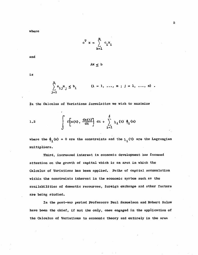
where
°T - ■ 1 V ik=l
and
is
Ax < b
\' a ,x ^ b, (i — 1, .«., in j j — lj > ■ • j n)L i «J J _ id=i
In the Calculus of Variations formulation we wish to maximize
I
1.2 * [* < « • 1 r ] d t + I * i ( t ) t ± wi=l
where the (J) (x) = 0 are the constraints and the (t) are the Lagrangian
multipliers.
Third, increased interest in economic development has focused
attention on the growth of capital which is an area in which the
Calculus of Variations has been applied. Paths of capital accumulation
within the constraints inherent in the economic system such as the
availabilities of domestic resources, foreign exchange and other factors
are being studied.
In the post-war period Professors Paul Samuelson and Robert Solow
have been the chief, if not the only, ones engaged in the application of
the Calculus of Variations to economic theory and entirely in the area
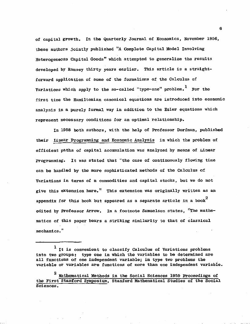
of capital growth. In the Quarterly Journal of Economics, November 1956,
these authors jointly published "A Complete Capital Model Involving
Heterogeneous Capital Goods” which attempted to generalize the results
developed by Ramsey thirty years earlier. This article is a straight
forward application of some of the formalisms of the Calculus of
Variations which apply to the so-called “type-one" problem.1 For the
first time the Hamiltonian canonical equations are introduced into economic
analysis in a purely formal way in addition to the Euler equations which
represent necessary conditions for an optimal relationship.
In 1958 both authors, with the help of Professor Dorfman, published
their Linear Programming and Economic Analysis in which the problem of
efficient paths of capital accumulation was analyzed by means of Linear
Programming. It was stated that "the case of continuously flowing time
can be handled by the more sophisticated methods of the Calculus of
Variations in terms of n commodities and capital stocks, but we do not
give this extension here.1' This extension was originally written as an2appendix for this book but appeared as a separate article in a book
edited by Professor Arrow. In a footnote Samuelson states, "The mathe
matics of this paper bears a striking similarity to that of classical
mechanics."
1 It is convenient to classify Calculus of Variations problems into two groups: type one in which the variables to be determined areall functions of one independent variable; in type two problems the variable or variables are functions of more than one independent variable.
2 Mathematical Methods in the Social Sciences 1959 Proceedings of the First Stanford Symposium, Stanford Mathematical Studies of the Social Sciences.
7
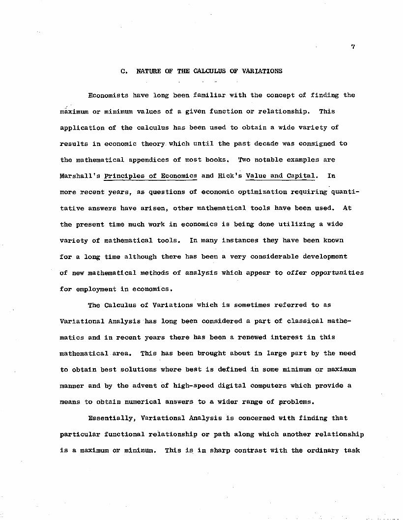
C. NATURE OF THE CALCULUS OF VARIATIONS
Economists have long been familiar with the concept of finding the
maximum or minimum values of a given function or relationship. This
application of the calculus has been used to obtain a wide variety of
results in economic theory, which until the past decade was consigned to
the mathematical appendices of most books. Two notable examples are
Marshall's Principles of Economics and Hick's Value and Capital. In
more recent years, as questions of economic optimization requiring quanti
tative answers have arisen, other mathematical tools have been used. At
the present time much work in economics is being done utilizing a wide
variety of mathematical tools. In many instances they have been known
for a long time although there has been a very considerable development
of new mathematical methods of analysis which appear to offer opportunities
for employment in economics.
The Calculus of Variations which is sometimes referred to as
Variational Analysis has long been considered a part of classical mathe
matics and in recent years there has been a renewed interest in this
mathematical area. This has been brought about in large part by the need
to obtain best solutions where best is defined in some minimum or maximum
manner and by the advent of high-speed digital computers which provide a
means to obtain numerical answers to a wider range of problems.
Essentially, Variational Analysis is concerned with finding that
particular functional relationship or path along which another relationship
is a maximum or minimum. This is in sharp contrast with the ordinary task
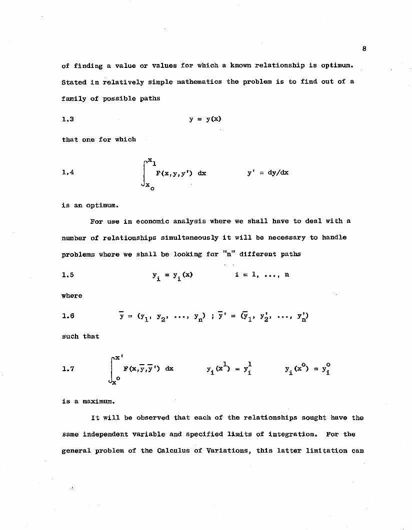
of finding a value or values for which a known relationship is optimum.
Stated in relatively simple mathematics the problem is to find out of a
family of possible paths
1.3 y = y(x)
that one for which
nxi1.4 PCxjy.y') dx y* = dy/dx
x
is an optimum.For use in economic analysis where we shall have to deal with a
number of relationships simultaneously it will be necessary to handle
problems where we shall be looking for "n" different paths
1.5 y± = y^x) i = 1, ..., n
where
1.6 y = (y1} y2, yQ) ; y' = (y^ y2, • ••* y )
such that
■>x11.7 F(x,y,y') dx y ^ x 1) = y^ yj.(x°) = y°
o*Jx
is a maximum.
It will be observed that each of the relationships sought have the
same independent variable and specified limits of integration. For the
general problem of the Calculus of Variations, this latter limitation can
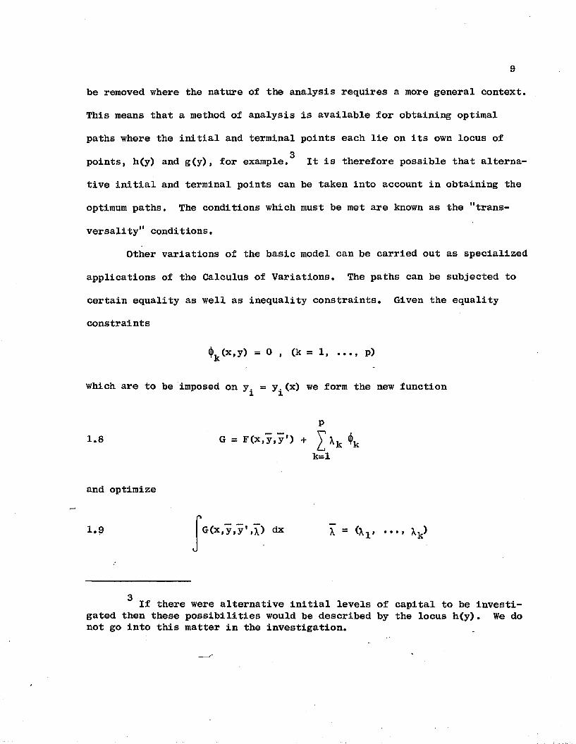
be removed where the nature of the analysis requires a more general context.
This means that a method of analysis is available for obtaining optimal
paths where the initial and terminal points each lie on its own locus of3points, h(y) and g(y), for example. It is therefore possible that alterna
tive initial and terminal points can be taken into account in obtaining the
optimum paths. The conditions which must be met are known as the "trans-
versality11 conditions.Other variations of the basic model can be carried out as specialized
applications of the Calculus of Variations. The paths can be subjected to
certain equality as well as inequality constraints. Given the equality
constraints
♦fc(x,y> = 0 > (k = 1, P)
which are to be imposed on y^ = y^(x) we form the new function
P1.8
k=l
and optimize
1.9 G(x,y,y\\) dx X = (Xx
3 If there were alternative initial levels of capital to be investigated then these possibilities would be described by the locus h(y). We do not go into this matter in the investigation.
10
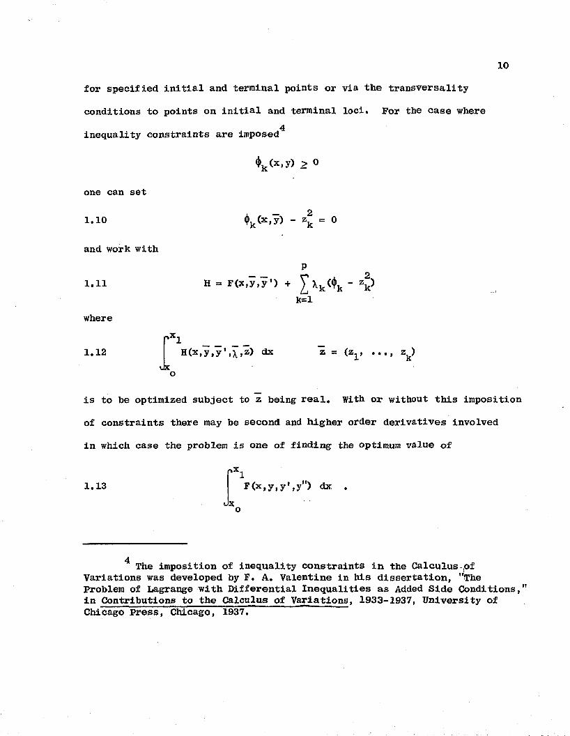
for specified initial and terminal points or via the transversality
conditions to points on initial and terminal loci. For the case where4inequality constraints are imposed
‘Lcx.y) > 0
one can set
1.10
and work with
^k(x,y) " Zk = 0
1.11
where
1.12rxi
H = F(x,y,y’) +k=l
H(x,y,y',x,z) dx Z - (Zj i . • • , Z )Ox
is to be optimized subject to z being real. With or without this imposition
of constraints there may be second and higher order derivatives involved
in which case the problem is one of finding the optimum value of
r>x.
1.13 F<x»y>y’»yn) dx .Ox
The imposition of inequality constraints in the Calculus -sof Variations was developed by F. A. Valentine in his dissertation, "The Problem of Lagrange with Differential Inequalities as Added Side Conditions," in Contributions to the Calculus of Variations, 1933-1937, University of Chicago Press, Chicago, 1937.
11
While it is possible that in the field of economics derivatives higher than
the first might be involved we shall not treat them.
From a purely mathematical standpoint there are a number of strong
requirements on the functions involved particularly regarding continuity
and differentiability which we shall assume. Necessary conditions to obtain
the optimal paths are well understood;, the use of the Weierstrass conditions
to determine sufficiency are more difficult and we shall not be concerned
with them.
In order to determine optimal paths of "n” simultaneous relationships
it will be necessary to work in "n" dimensional space. On occasion by
doubling the size of the space to 2n it will be possible to exhibit funda
mental relationships which are otherwise not obvious. This is accomplished
at the expense of adding to the computational burden. This more powerful
method of mathematical analysis, which came from the genius of W. R. Hamilton,
has a special significance for economic analysis which we shall utilize to
obtain our main results.
D. THE TRANSFORMATION FUNCTION OR LOCUS5
1. Role in Economic Analysis
For a number of years mathematical economists have utilized
the concept of a transformation locus in the theoretical analysis of the
firm. In this type of analysis it is assumed that the firm can produce two
g This discussion borrows from R. G. D. Allen's two books, Mathematical Analysis for Economists, Macmillan, 1938, and Mathematical Economics, St. Martins Press, 1956.
or more products X , X , . X with given supplies of factors of production.l a nAt this stage of the discussion we shall limit the number of products which
can be produced by a firm to two, X,Y, for purposes of easier exposition.
The results can be generalized to n products in a straightforward manner.
With the production of an amount x of X the fixed resources can be used for
the production of the greatest amount y of Y compatible with the production
of X. It is taken as normal that at higher levels of output of X the output
of Y will decrease at a faster rate and the reverse arguments would also
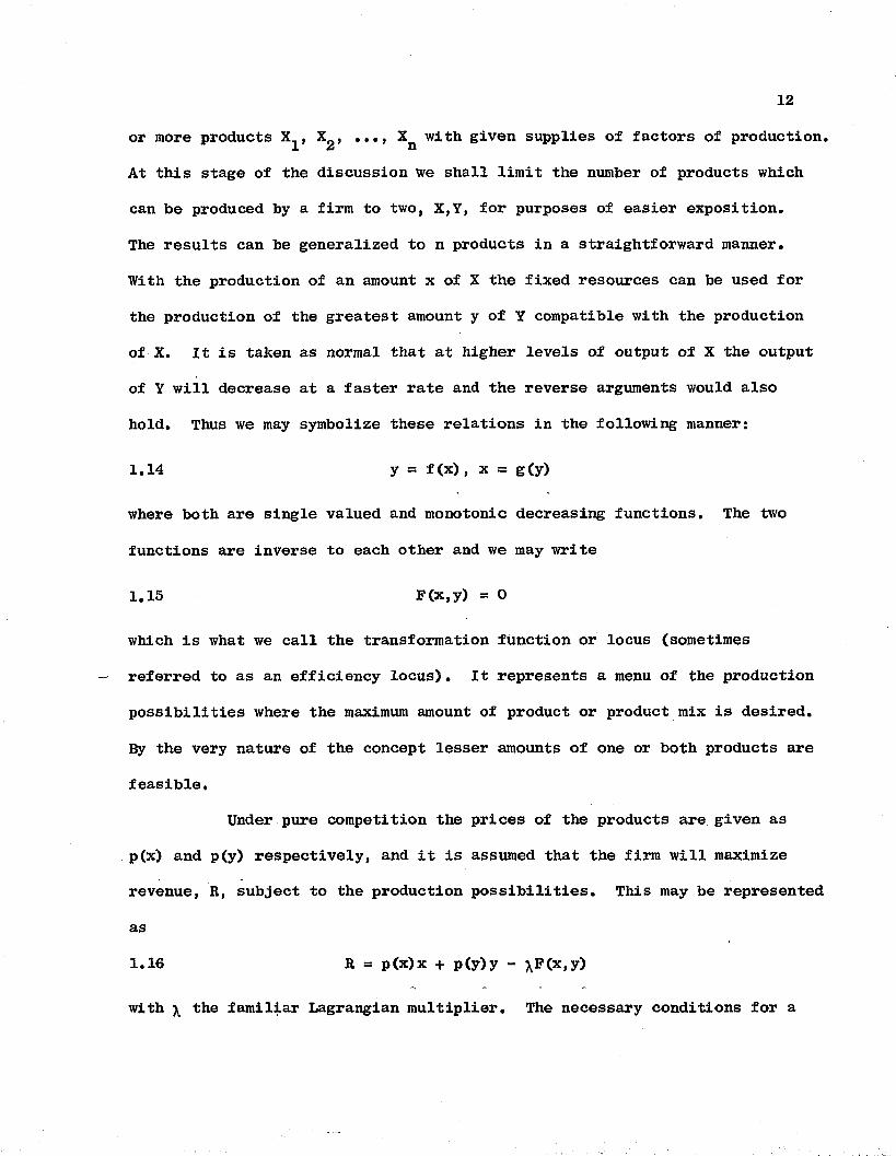
hold. Thus we may symbolize these relations in the following manner:
1.14 y = f (x) , x = g(y)
where both are single valued and monotonic decreasing functions. The two
functions are inverse to each other and we may write
1.15 F(x,y) = 0
which is what we call the transformation function or locus (sometimes
referred to as an efficiency locus). It represents a menu of the production
possibilities where the maximum amount of product or product mix is desired.
By the very nature of the concept lesser amounts of one or both products are
feasible.Under pure competition the prices of the products are given as
p(x) and p(y) respectively, and it is assumed that the firm will maximize
revenue, R, subject to the production possibilities. This may be represented
as
1.16 R = p(x)x + p(y)y - \F(x,y)
with \ the familiar Lagrangian multiplier. The necessary conditions for a
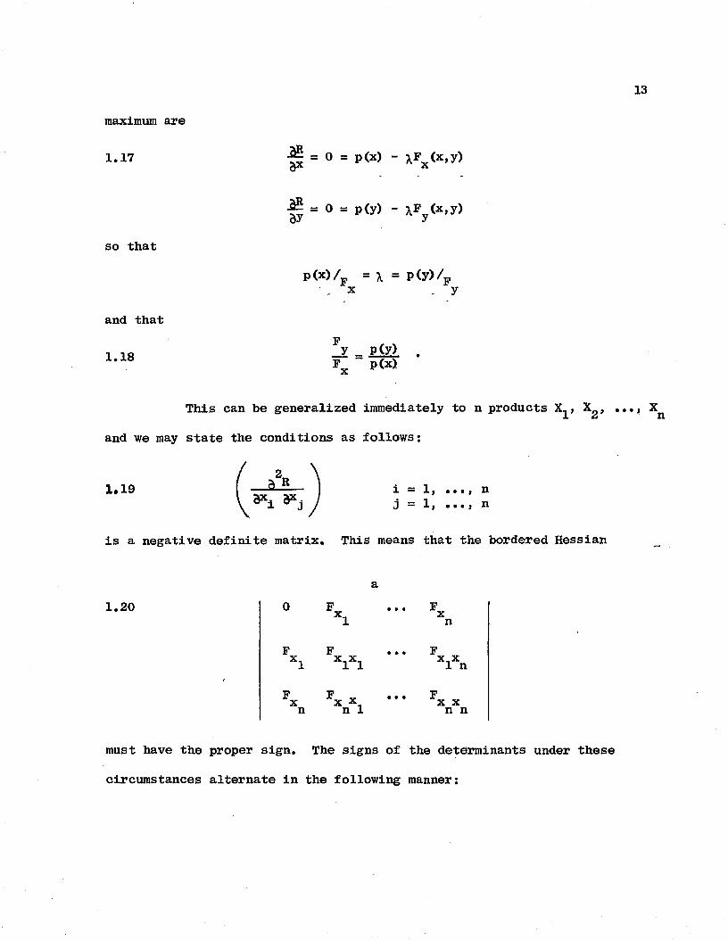
maximum are
1.17 = 0 = p(x) - xFx (x,y)
so that
= ° = P(y) - XFy(x,y)
p(x)/p = X = p(y)/jX
and that
1.18 _y _ p(y) .f x p(x)
This can be generalized immediately to n products X^, X^,
and we may state the conditions as follows:
1.19 _a!L
is a negative definite matrix. This means that the bordered Hessian
1.20 x.
X1X1
X X Xn n 1
n
x,x 1 n
X Xn n
must have the proper sign. The signs of the determinants under these
circumstances alternate in the following manner:
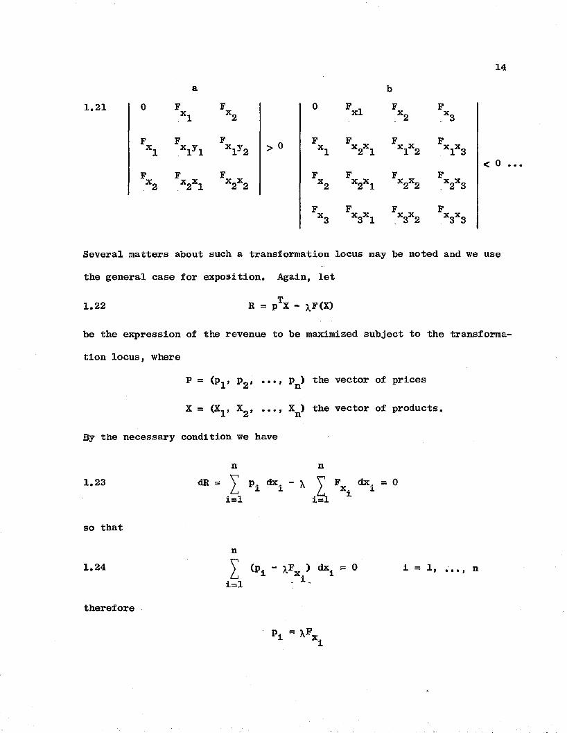
Several matters about such a transformation locus may be noted and we use
the general case for exposition. Again, let
be the expression of the revenue to be maximized subject to the transforma
tion locus, where
P = (P-. > P m •••» P ) the vector of prices l & n
X = (X , X2, ..., Xn) the vector of products.
By the necessary condition we have
1.22 R = pTX - xF(X)
n n1.23
i=lP dx. = 0x. 1ii=l
so that
n1.24
i=JL
therefore
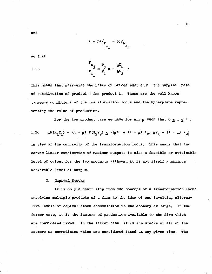
so that
This means that pair-wise the ratio of prices must equal the marginal rate
of substitution of product j for product i. These are the well known
tangency conditions of the transformation locus and the hyperplane repre
senting the value of production.
For the two product case we have for any jj, such that 0 < jj, < 1 .
1.26 uPOCjYj) + (1 - (J.) F(X2Y2) < F + (1 - |i) X2> ^ + (1 - ji) Y2]
in view of the concavity of the transformation locus. This means that any
convex linear combination of maximum outputs is also a feasible or attainable
level of output for the two products although it is not itself a maximum
achievable level of output.
2. Capital Stocks
It is only a short step from the concept of a transformation locus
involving multiple products of a firm to the idea of one involving alterna
tive levels of capital stock accumulation in the economy at large. In the
former case, it is the factors of production available to the firm which
are considered fixed. In the latter case, it is the stocks of all of the
factors or commodities which are considered fixed at any given time. The
16
problem then is the growth of these capital stocks during the next periodg
of time. One difference does arise, however, from the fact that a given
stock of capital will generate economic activity supporting consumption as
well as further growth of capital. The transformation locus therefore
includes consumption of such capital good as well as further stocks of each
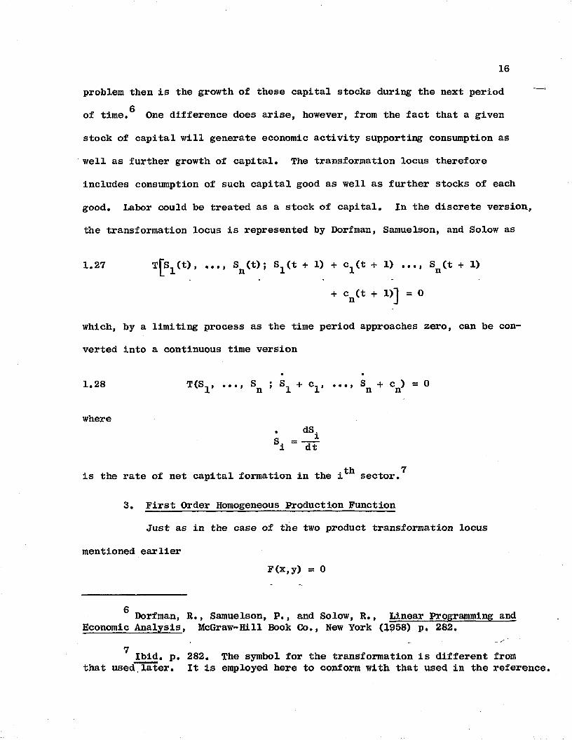
good. Labor could be treated as a stock of capital. In the discrete version,
the transformation locus is represented by Dorfman, Samuelson, and Solow as
1.27 Tfs. (t), ..., S (t); S (t + 1) + c (t + 1) ..., S (t + 1)1 n l l n+ cfl(t + l)j = 0
which, by a limiting process as the time period approaches zero, can be con
verted into a continuous time version
• •
1.28 T(S^, ..., Sn i S1 + c^i i•.i Sn + c^) = 0
wheredS
S, = -rf i dt
th 7is the rate of net capital formation in the i sector.
3. First Order Homogeneous Production Function
Just as in the case of the two product transformation locus
mentioned earlierF(x,y) = 0
gDorfman, R., Samuelson, P., and Solow, R., Linear Programming and
Economic Analysis, McGraw-Hill Book Co., New York (1958) p. 282.7 Ibid. p. 282. The symbol for the transformation is different from
that used.later. It is employed here to conform with that used in the reference.
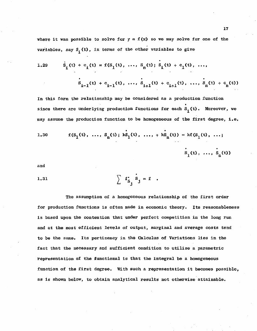
where it was possible to solve for y = f(x) so we may solve for one of the
variables, say S^t), in terms of the other variables to give
In this form the relationship may be considered as a production function
since there are underlying production functions for each S^(t). Moreover, we
may assume the production function to be homogeneous of the first degree, i.e.
for production functions is often made in economic theory. Its reasonableness
is based upon the contention that under perfect competition in the long run
and at the most efficient levels of output, marginal and average costs tend
to be the same. Its pertinency in the Calculus of Variations lies in the
fact that the necessary and sufficient condition to utilize a parametric
representation of the functional is that the integral be a homogeneous
function of the first degree. With such a representation it becomes possible,
as is shown below, to obtain analytical results not otherwise attainable.
1.29 • • • 9
1.30
s1(t), ..., sn(t))
and
1.31
The assumption of a homogeneous relationship of the first order
CHAPTER XI
MODELS1 OF ECONOMIC GROWTH IN THE
RECENT HISTORY OF ECONOMIC IDEAS
A. GENERAL VIEWS
In this chapter we shall investigate the role which capital accumula
tion has played in recent years in the formulation of models of economic
growth and place the concept of efficient paths of capital accumulation in
perspective. We shall be able to show the tradition out of which this
latter concept has grown and therefore place our analysis in its proper
historical setting. While the question of the nature and role of capital
has been a subject of investigation at least since the days of Adam Smith,
we shall confine our attention primarily to the period since World War II
with one or two notable exceptions, but we must recognize that the question
of economic growth and the role of capital was one of the principal concerns
of Ricardo.... The extension of the classical analysis by Marx is too familiar
to need any elaboration. Toward the end of the 19th century the subject of
capital was again an object of investigation by BHhm-Bawerk and J. B. Clark.
Since we are dealing with efficient paths of capital accumulation
and much of the economic literature is in terms of growth models we must be
clear about the meanings we ascribe to these concepts. In the literature,
growth is generally taken to mean the rise in national income (or one of the
related magnitudes such as Gross National Product) but it could just as well
1 The word model is used to indicate a formal framework within which to carry out the economic analysis.
19
be represented by the rise of the total output of the economy. Moreover,
it can be on a total value basis, a per man basis or even on a per hour
basis, although the latter is frequently a measure of productivity. When a
total value basis is used it is generally in real terms or constant dollars
so that monetary considerations do not enter into the analysis. By carrying
out the analysis in terms of a per man basis the growth in the population
or labor force is brought into the analysis. But what is of particular
interest is the fact that growth as it has been used is an aggregate concept
covering the entire economy rather than growth of an industry or particular
sector such as steel, automobile, weaving or textiles. The nature of growth
is also subject to varying interpretations. From one point of view it could
be understood to mean the most rapid rate of growth possible although this
would have to be subject to certain types of constraints otherwise consumption,
the government sector and the foreign trade sectors would be called upon to
undergo unacceptable deprivations. Other yardsticks for measuring growth
could involve the question of maintaining full employment of capital resources
as well as labor. Still another concept might be that rate of growth which
is consistent with the saving and investing patterns of activity of the
entrepreneurial class. Regardless of which concept is of interest the
determinants of the growth rate are inherent in the economic structure and
are in a sense market oriented although it is of course true that the govern
ment is not without resources to exert direct or indirect influence over
economic growth.
On the other hand efficient paths of capital accumulation will be
understood to refer to investment, on a net basis, in one or more specified
industrial sectors, in contrast to the path through time of some measure of
20
overall economic activity such as total production, indicated in the above
paragraph. How the sector or sectors are selected is not the critical
issue but the fact that there is some central control involved is what is
required. The objective might be the build-up of the fertilizer industry
as an example and the goal to be achieved would be to reach some specified
level of capacity in the particular industry. Of course, as is true for
the aggregate analysis referred to previously, resources are limited for
the case under consideration. Resources devoted -to the build-up of a given
industry or industries must be obtained at the expense of other industries,
consumption, government activities or such other economic activities as
might be involved.
What we are concerned with is known in the literature as a multi
sector model of the economy in which all the relevant sectors are included
in the analysis. This is in sharp contrast to the aggregate type models
where total levels of production, consumption, investment and government
spending are involved. It is the maximization of investment in a particular
sector which is to be achieved with the other sectors a central part of
the analysis. Within such a framework efficient paths of capital accumula
tion will not only involve the sector whose path is to be maximized but
also the paths of the other sectors of the economy. Their pattern of growth
is such that the necessary conditions of the Euler-Lagrange equations are
satisfied. Moreover, all the paths including the one which is maximized
must satisfy the fundamental relationship between the various own rates of
interest, which we shall briefly consider in the next chapter although it
is not the main focus of attention in this study.
21
The kind of problem to which this analysis addresses itself is
similar to what a developing country faces after having decided what sectors
must be developed first. The model with which we are concerned, however,
presents an idealized pattern of what could be accomplished within the
constraints imposed; it does not purport to represent a realistic situation
that one might find in an economy. As in so much of economic theorizing it
has the possibility of giving some added insights into the growth problem.
We shall see that the kind of analysis to be undertaken springs from
two separate but related traditions in the development of economic ideas,
both of relatively recent origin. In both traditions it is recognized that
economic growth, however defined, can be brought about or at least influenced
by many factors including institutional arrangements, development of tech
nology, productivity of labor, changes in consumers preferences, monetary
factors and changes in expectations. However, it is the essence of economic
theory to be able to select out from the welter of detail those factors which
can be identified as being the main motors in providing the thrust of the
economy. This is especially true in the macro-economic field although it
brings with it problems involving the degree of aggregation, measurement,
errors in the data, comparability of information and a host of other diffi
culties which make the testing of hypotheses about economic activity
troublesome. But all this is nothing new in either the micro or macro
economic theories which economists have expounded to bring about greater
understanding of the nature of economic activity.
22
B. a g g r e g a t e e c o n o m i c m o d e l a n d ec o n o m i c g r o w t h
The post World War II period has witnessed an unprecedented amount
of theoretical analysis in the formulation of economic models describing
paths and levels of economic activity. The pioneering work was done by2Harrod in an article published just prior to the outbreak of the war and
slightly recast and enlarged in a series of lectures which appeared in book
form in 1948 under the title, Towards A Dynamic Economics. There have been3 4a number of suggested modifications associated with Domar , Baumol ,
5 6 7 8 9 10Alexander , Hicks , Duesenberry , Phillips , Goodwin , and Samuelson .
2 Harrod, Roy F., "An Essay in Dynamic Theory," Economic Journal,1939. See also Towards A Dynamic Economics, Macmillan, 1949.
Domar, Evsey D., "Capital Expansion, Rate of Growth and Employment,"Econometrica, Vol. 14, p. 137-147. See also his Essays in the Theory of Economic Growth.
^ Baumol, William J., "Formalization of Mr. Harrod's Model," Economic Journal, Vol. 59 (1949). See.also Economic Dynamics, Macmillan, 1951.
g Alexander, Sydney, "Mr. Harrod's Dynamic Model," Economic Journal Vol. 60 (1950).
0 Hicks, J. R., A Contribution to the Theory of the Trade Cycle,Oxford Clarendon Press, 1959.
7 Duesenberry, James J., "Hicks on the Trade Qycle," Quarterly Journal of Economics, Vol. 64 (1950).
Phillips, W. A., "Stabilization Policy in a Closed Economy," Economic Journal, Vol. 64 (1950).
9 Goodwin, R. M., The Non-Linear Accelerator and the Persistence of Business Cycles," Econometrica, Vol. 19.
10 „Samuelson, Paul A., Interactions between the Multiplier Analysisand the Principle of Acceleration," Review of Economic Statistics, Vol. 21.
By and large the differences or modifications described in the literature
tend to be matters of detail in terms of our main interest. They involve
such issues as continuous versus period analysis, the number of time lags
to be incorporated in the consumption, savings and investment relationships,
the expected path of autonomous investment, and the linearity of such
relationships. It is of particular interest to note that in none of these
articles is there any attempt to identify their theoretical developments
with the work of such eminent economic theorists as Schumpeter’1-'1' or Joan 12Robinson even though the latter two had been active in the field of
economic development as early as the decade of the '30's. If there was
any real source it was Keynes and the "General Theory" but mainly as a point
of departure, for his is essentially a static equilibrium model with no
attempt at analyzing the paths of economic activity through time. One of
his basic conclusions that there can be equilibrium at less than full
utilization of labor typifies his general approach. However, the focus of
his attention on the role of investment and the consumption relationship
had a profound impact on the work of Harrod, Domar and others. But Keynes
never had a concept involving the accelerator which relates induced invest
ment to changes in income levels and it was therefore not to be expected
that his model would be dynamic in the sense that the growth in income would
Schumpeter, Joseph, The Theory of Economic Development, Harvard University Press, Cambridge, Mass., 1934.
12 Robinson, Joan, Accumulation of Capital
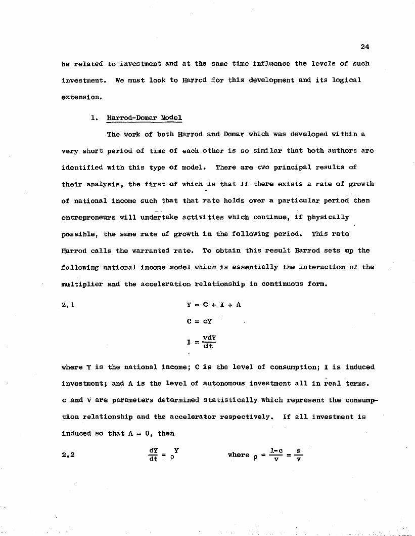
be related to investment and at the same time influence the levels of such
investment. We must look to Harrod for this development and its logical
extension.
1. Harrod-Domar ModelThe work of both Harrod and Domar which was developed within a
very short period of time of each other is so similar that both authors are
identified with this type of model. There are two principal results of
their analysis, the first of which is that if there exists a rate of growth
of national income such that that rate holds over a particular period then
entrepreneurs will undertake activities which continue, if physically
possible, the same rate of growth in the following period. This rate
Harrod calls the warranted rate. To obtain this result Harrod sets up the
following national income model which is essentially the interaction of the
multiplier and the acceleration relationship in continuous form.
2.1 Y = C + I A
C = cY
vdYdt
where Y is the national income; C is the level of consumption; 1 is induced
investment; and A is the level of autonomous investment all in real terms,
c and v are parameters determined statistically which represent the consump
tion relationship and the accelerator respectively. If all investment is
induced so that A = 0, then
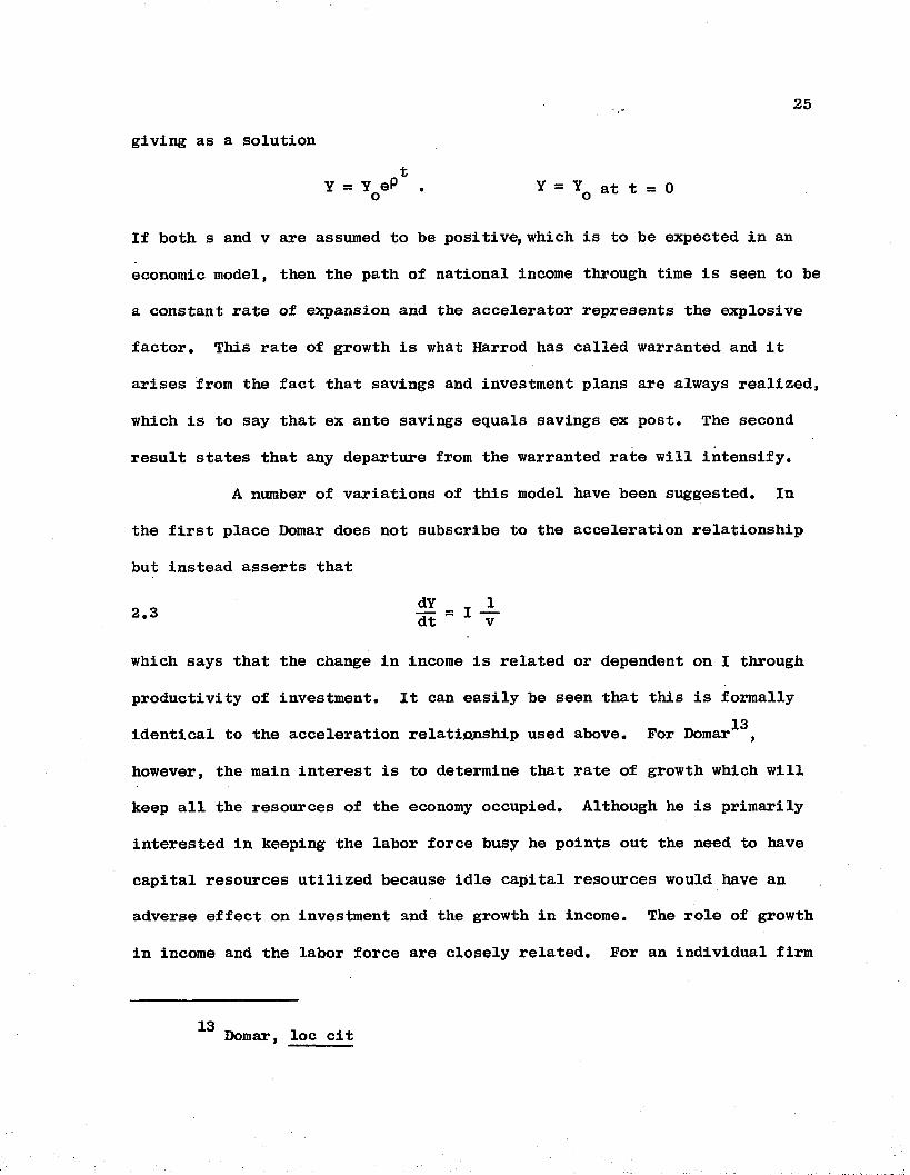
giving as a solutiont
Y = YQeP . Y = Yq at t = 0
If both s and v are assumed to be positive, which is to be expected in an
economic model, then the path of national income through time is seen to be
a constant rate of expansion and the accelerator represents the explosive
factor. This rate of growth is what Harrod has called warranted and it
arises from the fact that savings and investment plans are always realized,
which is to say that ex ante savings equals savings ex post. The second
result states that any departure from the warranted rate will intensify.
A number of variations of this model have been suggested. In
the first place Domar does not subscribe to the acceleration relationship
but instead asserts that
which says that the change in income is related or dependent on I through
productivity of investment. It can easily be seen that this is formally13identical to the acceleration relationship used above. For Domar ,
however, the main interest is to determine that rate of growth which will
keep all the resources of the economy occupied. Although he is primarily
interested in keeping the labor force busy he points out the need to have
capital resources utilized because idle capital resources would have an
adverse effect on investment and the growth in income. The role of growth
in income and the labor force are closely related. For an individual firm
13 Domar, loc cit
26
investment may mean more capital and less labor but for the economy as a
whole investment means more capital and not less labor. If both are to
be profitably employed a growth in income must take place.
In its continuous form as originally presented, the Harrod-Domar
model is not dynamic in view of the fact that no provision is made for
unintended investment or saving. By introducing lags in the acceleration
relationship and providing for the possibility that investment plans may14 15not be realized the model has been made dynamic by Raumol and Alexander .
It then becomes necessary to specify a particular kind of response to a
deficiency in investment. But in such a situation the warranted rate of
growth ceases to have much meaning and the time path of total output or
income may be damped, explosive or oscillatory, depending upon the
structural constants in the model. Additional modifications have been
introduced depending upon what is assumed by the pattern of autonomous
investment through time. By assuming a constant rate of growth in such
investment which appears to be a heroic assumption the levels of national
income can be shown to oscillate around an equilibrium level. All of this
indicates that any aggregate model in which savings plans are realized do
not give rise to activity which appears reasonable from an economic point
of view and especially when the idea of a warranted rate of growth is
involved.
^ Baumol, loc cit
Alexander, loc cit
27
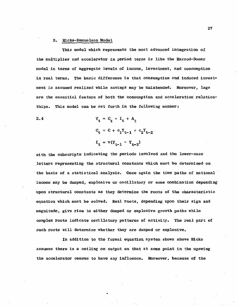
2. Hicks-Samuelson Model
This model which represents the most advanced integration of
the multiplier and accelerator in period terms is like the Harrod-Domar
model in terms of aggregate levels of income, investment, and consumption
in real terms. The basic difference is that consumption and induced invest
ment is assumed realized while savings may be unintended. Moreover, lags
are the essential feature of both the consumption and acceleration relation-
thips. This model can be set forth in the following manner;
2.4 Yt = ct + It + At
Ct = C + ClYt-l + C2Yt-2
't = V<Yt-X - Yt-2>
with the subscripts indicating the periods involved and the lower-case
letters representing the structural constants which must be determined on
the basis of a statistical analysis. Once again the time paths of national
income may be damped, explosive or oscillatory or some combination depending
upon structural constants as they determine the roots of the characteristic
equation which must be solved. Real roots, depending upon their sign and
magnitude, give rise to either damped or explosive growth paths while
complex roots indicate oscillatory patterns of activity. The real part of
such roots will determine whether they are damped or explosive.
In addition to the formal equation system shown above Hicks
assumes there is a ceiling on output so that at some point in the upswing
the accelerator ceases to have any influence. Moreover, because of the
existence of excess capital on the downswing the value of the accelerator
is assumed to be smaller during that part of the cycle. This model has
been subjected to constructive criticism by Duesenberry who argues that
disinvestment is limited by size of depreciation allowances. At the bottom
there are new initial conditions for the start of the upswing. With the
existence of excess capacity the accelerator will not be effective. In
fact, each cycle starts with the elimination of excess capacity. The
ceiling is called into question because a steady cyclic pattern can be
maintained even if the multiplier and accelerator coefficients imply
explosive oscillatory cycles. Finally, Duesenberry suggests the replace
ment of a rising trend of autonomous investment with an irreversible
consumption function which keeps the income in a depression from falling
back to the level of a previous depression.
In the search for more adequate models to describe both the growth
of the economy and its cyclical behaviour, many variations of the basic
relationships described in the above two models have been developed. The
most notable have been those due to Phillips and Goodwin, with the former
introducing lags in the continuous version while the latter makes use of a
non-linear accelerator. There has been much interest in these models not
only because of the people associated with them but also because the
question of growth has become more important. However, there is dissatis
faction with the idea that a warranted rate of growth rests upon a razor's
edge and once off will depart farther and farther from such a rate. More
over, the statistical evidence of the existence of the accelerator is not
too convincing even with the modifications introduced by Duesenberry and
others. The question that arises is how useful is the aggregated model in
explaining the pattern of growth for individual sectors of the economy. It
seems reasonably clear that the total value of output is a resultant of many
diverse movements in the individual industries, and the level of aggregation
may mask the important movements. For planning purposes the disadvantages
are even greater. Not everything is equally important in any development
program: services and agriculture may not be in the proper relationship to
the industrial sectors. For a partial answer to this type of question we
shall consider more recent developments in the area of growth models.
C. MULTISECTOR ECONOMIC GROWTH MODELS
The adaptation and further development of the concept of economic
growth to many sectors of the economy has been the subject of much recent
analysis. While it represents in one sense a logical extension of the work
done for aggregate analysis, a considerable part of the motivation has come
from a different tradition in which the pioneering work was done by Ramsey
as indicated earlier. This work, interestingly enough, was also couched in
aggregate terms with its main focus the question of how much an economy
should save. With this determined, at least conceptually, the question was
then raised as to how to distribute these resources among the different
sectors of the economy to achieve economic growth. The Calculus of Variations
has played an increasingly important role in this kind of analysis.
30
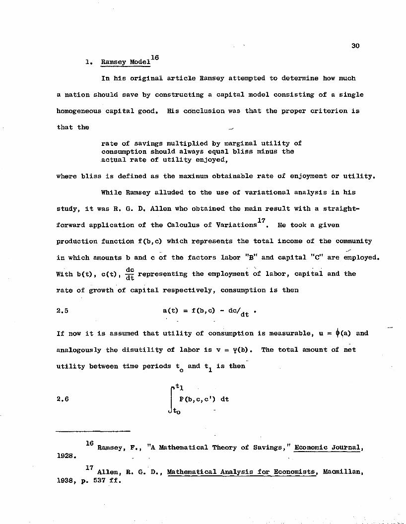
1. Ramsey Model^
In his original article Ramsey attempted to determine how much
a nation should save by constructing a capital model consisting of a single
homogeneous capital good. His conclusion was that the proper criterion is
that the
rate of savings multiplied by marginal utility of consumption should always equal bliss minus the actual rate of utility enjoyed,
where bliss is defined as the maximum obtainable rate of enjoyment or utility.
While Ramsey alluded to the use of variational analysis in his
study, it was R. G. D. Allen who obtained the main result with a straight-17forward application of the Calculus of Variations . He took a given
production function f(b,c) which represents the total income of the community
in which amounts b and c of the factors labor "b " and capital MCM are employed, dcWith b(t), c(t), representing the employment of labor, capital and theQX
rate of growth of capital respectively, consumption is then
2.5 a(t) = f(b,c) - de/dt .
If now it is assumed that utility of consumption is measurable, u = <j>(a) and analogously the disutility of labor is v = y(b). The total amount of net
utility between time periods tQ and ^ is then
f l2.6 F(b,c,c’) dt
to
10 Ramsey, F., ,rA Mathematical Theory of Savings," Economic Journal,1928.
17 Allen, R. G. D., Mathematical Analysis for Economists, Macmillan, 1938, p. 537 ff.
31
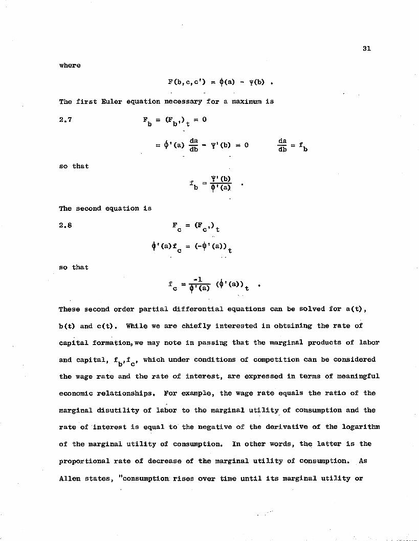
where
F(b,c,c') = <jl(a) - y(b) •
The first Euler equation necessary for a maximum is
2.7 Fb = <Fb,)t . 0
= (f)» (a) — - v» (b) = 0 — = f.V w db * v ' db b
so thaty(b)
b (f>' (a) *
The second equation is
2.8 Fc = (Fo,)t
♦ '<“>*, = <-+'(a))t
so that
These second order partial differential equations can be solved for a(t),
b(t) and c(t). While we are chiefly interested in obtaining the rate of
capital formation, we may note in passing that the marginal products of labor
and capital, f^,fc> which under conditions of competition can be considered
the wage rate and the rate of interest, are expressed in terms of meaningful
economic relationships. For example, the wage rate equals the ratio of the
marginal disutility of labor to the marginal utility of consumption and the
rate of interest is equal to the negative of the derivative of the logarithm
of the marginal utility of consumption. In other words, the latter is the
proportional rate of decrease of the marginal utility of consumption. As
Allen states, "consumption, rises over time until its marginal utility or
32
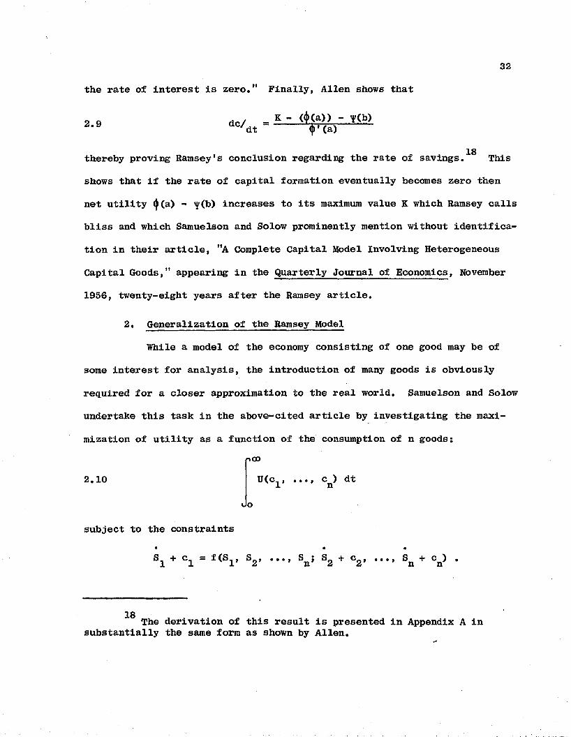
the rate of interest is zero." Finally, Allen shows that
2.9 dc/dt_ K - <<!» (a)) - y(b)"ip—
thereby proving Ramsey’s conclusion regarding the rate of savings 18 This
shows that if the rate of capital formation eventually becomes zero then
net utility <|)(a) - increases to its maximum value K which Ramsey calls
bliss and which Samuelson and Solow prominently mention without identifica
tion in their article, "A Complete Capital Model Involving Heterogeneous
Capital Goods," appearing in the Quarterly Journal of Economics, November
1956, twenty-eight years after the Ramsey article.
2. Generalization of the Ramsey Model
some interest for analysis, the introduction of many goods is obviously
required for a closer approximation to the real world. Samuelson and Solow
undertake this task in the above-cited article by investigating the maxi
mization of utility as a function of the consumption of n goods:
While a model of the economy consisting of one good may be of
2.10 U(c,, ..., c ) dt 1 n«Jo
subject to the constraints
18 The derivation of this result is presented in Appendix A in substantially the same form as shown by Allen.
33
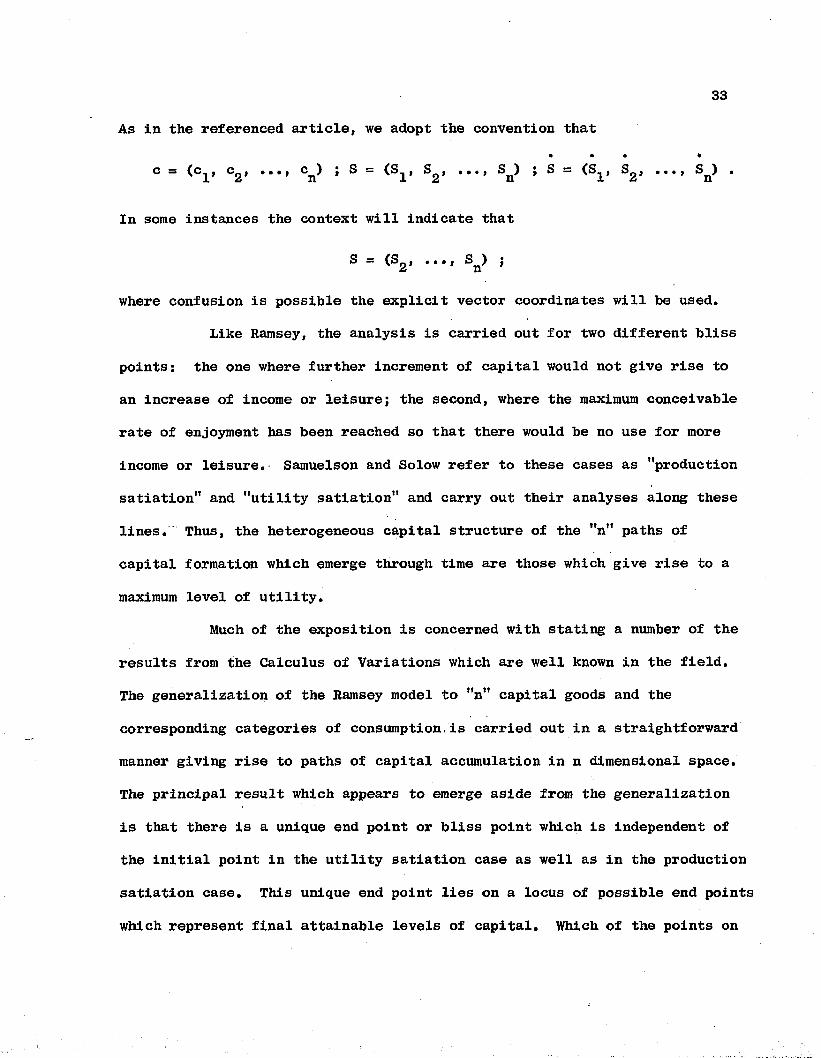
As in the referenced article, we adopt the convention that• • • *
c ss (c-» C2 * ; S = (S^, S^j •••» Sn) } S = (S^i Sg, • • •, sn) •
In some instances the context will indicate that
s = (Sg, •••, Sn) j
where confusion is possible the explicit vector coordinates will be used.
Like Ramsey, the analysis is carried out for two different bliss
points: the one where further increment of capital would not give rise to
an increase of income or leisure; the second, where the maximum conceivable
rate of enjoyment has been reached so that there would be no use for more
income or leisure. Samuelson and Solow refer to these cases as ’’production
satiation" and "utility satiation" and carry out their analyses along these
lines. Thus, the heterogeneous capital structure of the "n" paths of
capital formation which emerge through time are those which give rise to a
maximum level of utility.
Much of the exposition is concerned with stating a number of the
results from the Calculus of Variations which are well known in the field.
The generalization of the Ramsey model to "n” capital goods and the
corresponding categories of consumption.is carried out in a straightforward
manner giving rise to paths of capital accumulation in n dimensional space.
The principal result which appears to emerge aside from the generalization
is that there is a unique end point or bliss point which is independent of
the initial point in the utility satiation case as well as in the production
satiation case. This unique end point lies on a locus of possible end points
which represent final attainable levels of capital. Which of the points on
34
the locus is the desired bliss point is determined by the transversality
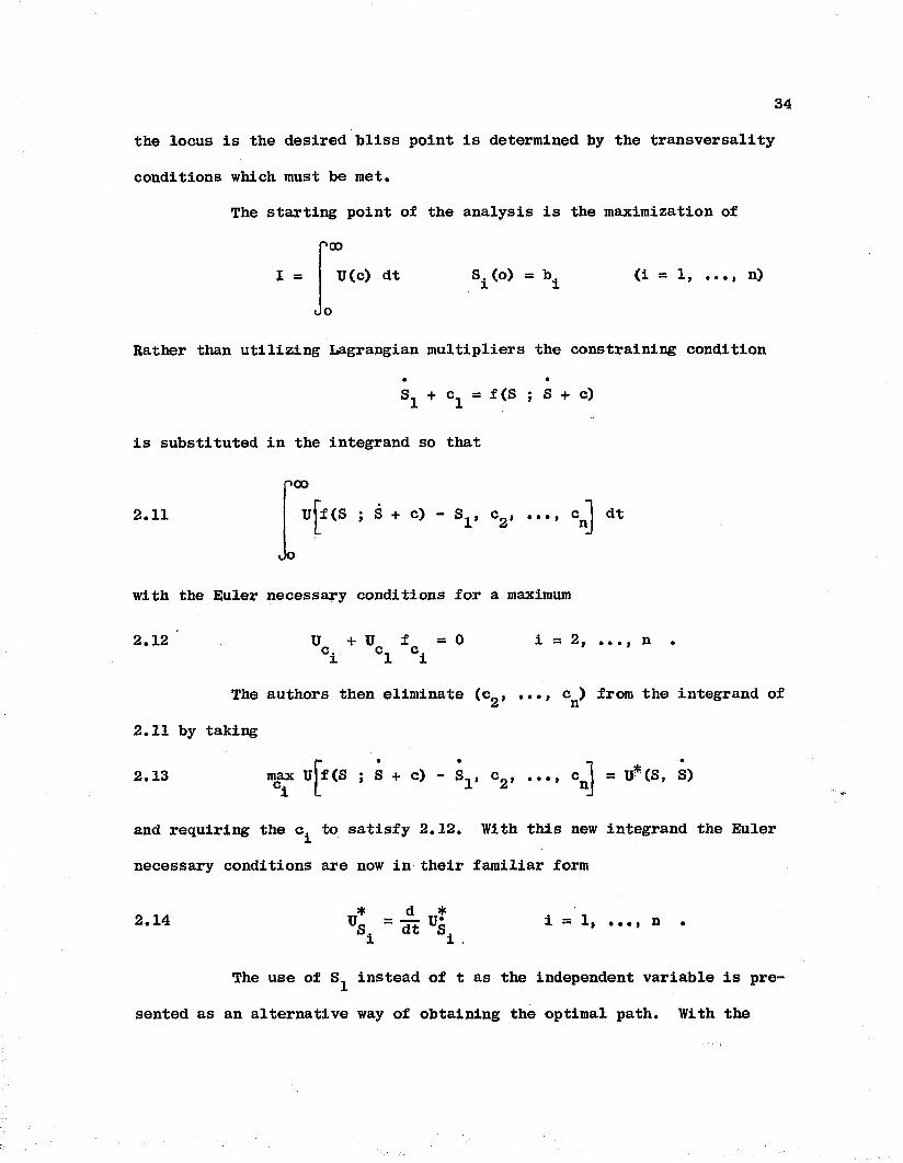
conditions which must be met.The starting point of the analysis is the maximization of
oooI = U(c) dt si<°> - \ (i = 11 ... i n)
do
Rather than utilizing Lagrangian multipliers the constraining condition
S1 + c = f(S ; S + c)
is substituted in the integrand so that
poo2.11 ujf(S j S + c) — S^, c^j •••» dt
Jo
with the Euler necessary conditions for a maximum
2.12 U + U f = 0 °i C1 °i
i — 2 j • • • y n •
The authors then eliminate (coJ . c ) from the integrand ofa n2.11 by taking
2.13 f. . — •
f(S ; S + c) - c2> ..., cnj = U*(S, S)
and requiring the c^ to satisfy 2.12. With this new integrand the Euler
necessary conditions are now in their familiar form
2.14 . * d * US± " dt \
The use of instead of t as the independent variable is pre
sented as an alternative way of obtaining the optimal path. With the
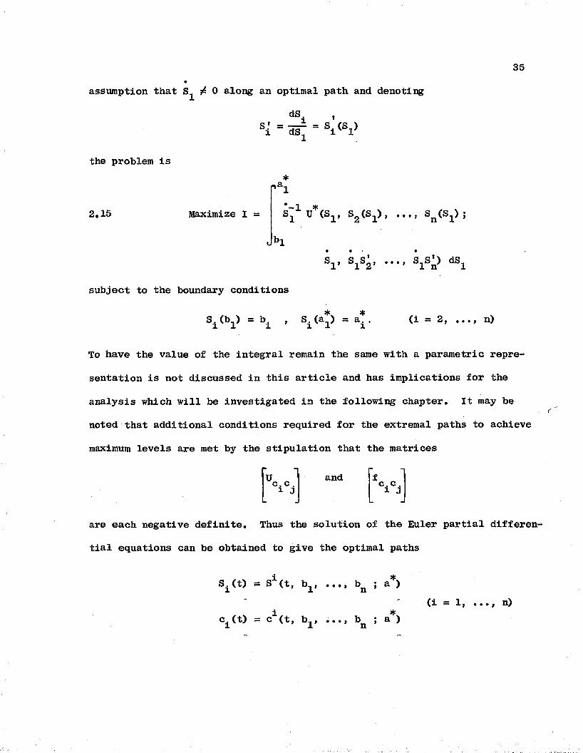
35
assumption that ^ 0 along an optimal path and denoting
dS
the problem is
2.15ra!
Maximize 1 = S11 U*(S1’ S2 (Sl)f V * 3!* 5
*>1• •
sl> sis2...... SlS'n> dsl
subject to the boundary conditions
Si*bl* = bi * ^i(a*) = a*. (i = 2, n)
To have the value of the integral remain the same with a parametric repre
sentation is not discussed in this article and has implications for the
analysis which will be investigated in the following chapter. It may bec
noted that additional conditions required for the extremal paths to achieve
maximum levels are met by the stipulation that the matrices
1Uc. c . i 3and c. c . i J
are each negative definite. Thus the solution of the Euler partial differen
tial equations can be obtained to give the optimal paths
S^t) = Si(t, b ^ ..., bn ; a*)
i *^(t) = c (t, bj, ..., b ; a )(i = 1, ..., n)
36
Some discussion of the model is devoted to (1) setting forth in
a purely mathematical manner some of the Hamiltonian equations which can
be obtained by working in a 2n dimensional space in which first order
partial differential equations are obtained, although these equations are
not used in the analysis, and (2) a very brief exposition of the famous_ rHamilton-Jacobi partial differential equation which can be used to get the
optimal paths of the problem. We shall go into these matters in some detail
in the following two chapters ascribing economic content to the results.
3. Efficient Paths of Capital Growth
The most recent contribution to the development of a Capital
Model using the Calculus of Variations as the principal means of analysis
is Professor Samuelson's article, "Efficient Paths of Capital Accumulation
in Terms of the Calculus of Variations,” which appeared as a chapter in
Mathematical Methods in the Social Sciences referred to earlier. It builds
on the earlier generalized Ramsey model and is at the same time a continuous
version of the discrete time analysis of Chapter 12, "Efficient Programs of
Capital Accumulation," of Linear Programming and Economic Analysis published
in 1958 by Dorfman, Samuelson and Solow. Rather than maximizing the utility
as in the generalized Ramsey case, the direct optimization of capital stocks
is undertaken subject, however, to the production function relationship as
in the earlier version.^
19 The authors point out that this formulation can be derived from the utility model previously described. See equations in Samuelson, P., and Solow, R., "A Complete Capital Model Involving Heterogeneous Capital Goods," Quarterly Journal of Economics, 70, (1956) p. 541.
37
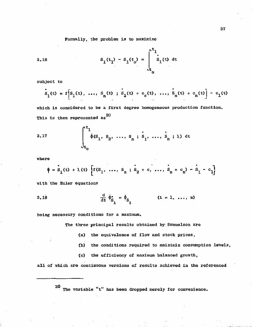
Formally, the problem is to maximize
:1rt’t-2.16 S,(t) dt
subject to
S^t) = f ^ C t ) , Sn (t) ; S2(t) + cg(t), Sn (t) + cn (t)j - ^(t)
which is considered to be a first degree homogeneous production function.20This is then represented as
pt.2.17
m •Sg, • •«> Sn j Slf ..., Sn j X) dt
where
<|> = Sx(t) + X(t) p c s 1> •••> j Sg + c
with the Euler equations
2.18 — ()>• = d)dt V , YS. (i — 1, ..., n)
being necessary conditions for a maximum.
The three principal results obtained by: Samuelson are
(a) the equivalence of flow and stock prices,
(b) the conditions required to maintain consumption levels,
(c) the efficiency of maximum balanced growth,
all of which are continuous versions of results achieved in the referenced
The variable "t" has been dropped merely for convenience.
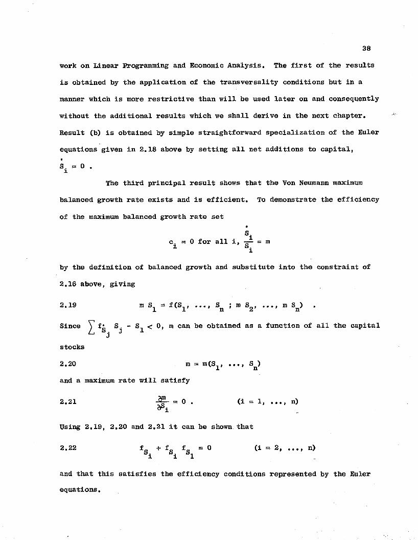
38
work on Linear Programming and Economic Analysis. The first of the results
is obtained by the application of the transversal!ty conditions but in a
manner which is more restrictive than will be used later on and consequently
without the additional results which we shall derive in the next chapter.
Result (b) is obtained by simple straightforward specialization of the Euler
equations given in 2.18 above by setting all net additions to capital,•S. = 0 .l
The third principal result shows that the Von Neumann maximum
balanced growth rate exists and is efficient. To demonstrate the efficiency
of the maximum balanced growth rate set•
Sic. = 0 for all i, —— = msi
by the definition of balanced growth and substitute into the constraint of
2.16 above, giving
2.19 m = f(S1, ..., ; m S^, ..., m S^)
Since V S. - S, < 0, m can be obtained as a function of all the capitalL s. j 1stocks
2.20 m — m(Sn, ..., S )1 nand a maximum rate will satisfy
2.21 -22- = 0 . (i = 1, ..., n)
Using 2.19, 2.20 and 2a21 it can be shown that
2.22 f + f f = 0 (i = 2, ..., n)i i 1
and that this satisfies the efficiency conditions represented by the Euler equations.
39
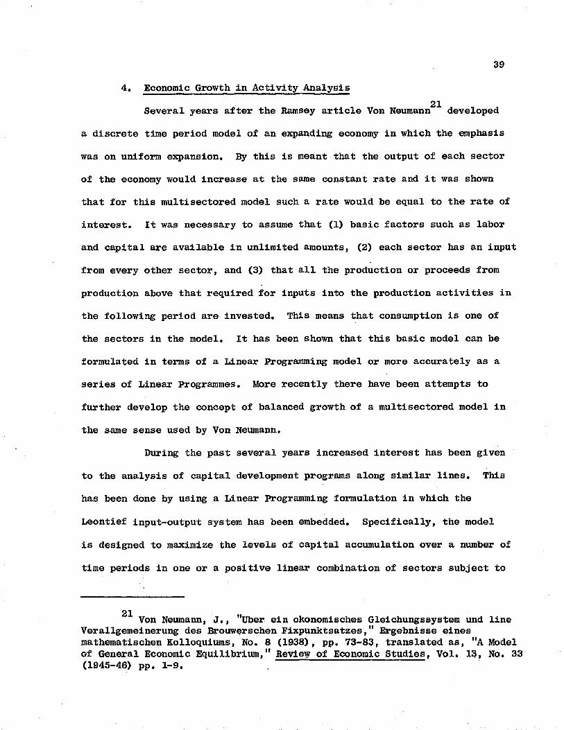
4. Economic Growth in Activity Analysis21Several years after the Ramsey article Von Neumann developed
a discrete time period model of an expanding economy in which the emphasis
was on uniform expansion. By this is meant that the output of each sector
of the economy would increase at the same constant rate and it was shown
that for this multisectored model such a rate would be equal to the rate of
interest. It was necessary to assume that (1) basic factors such as labor
and capital are available in unlimited amounts, (2) each sector has an input
from every other sector, and (3) that all the production or proceeds from
production above that required for inputs into the production activities in
the following period are invested. This means that consumption is one of
the sectors in the model. It has been shown that this basic model can be
formulated in terms of a Linear Programming model or more accurately as a
series of Linear Programmes. More recently there have been attempts to
further develop the concept of balanced growth of a multisectored model in
the same sense used by Von Neumann.
During the past several years increased interest has been given
to the analysis of capital development programs along similar lines. This
has been done by using a Linear Programming formulation in which the
Leontief input-output system has been embedded. Specifically, the model
is designed to maximize the levels of capital accumulation over a number of
time periods in one or a positive linear combination of sectors subject to
21 Von Neumann, J., "Uber ein okonomisches Gleichungssystem und line Verallgemeinerung des Brouwerschen Fixpunktsatzes," Ergebnisse eines mathematischen Kolloquiums, No. 8 (1938), pp. 73-83, translated as, "A Model of General Economic Equilibrium,1* Review of Economic Studies, Vol. 13, No. 33 (1945-46) pp. 1-9.
40
capacity restraints. The variables for this formulation represent levels of
capital in the various sectors by time period.
It can be seen that this approach represents a significant
departure from what has been described above in connection with aggregate
analysis. First of all it is non-market-oriented by which is meant that the
interplay of prices, consumption, and the levels of income do not have an
impact on investment activities. Levels of investment are determined on the
basis of technological considerations involving the individual sector input-
output relations and the capital-output ratios. Consumption of sector output
by consumers by time periods generally is stipulated.
The solution of such a Linear Programming model generates levels
of capital accumulation in quantity terms which maximize one sector or some
positive combination of sectors. The question naturally arises as to the role
of prices in such a formulation. It is well known that there is a dual
solution to every regular or primal solution to a Linear Programming model,
the variables of which are prices of the resources employed in the model.
Such prices are variously described as shadow prices or accounting prices
associated with the resources utilized. The prices of resources which are
not fully utilized are zero, the prices of fully utilized resources being
positive. A set of such prices may not be unique. They can be interpreted
as rates of substitution and in competitive markets may be thought of as
market prices. In non-competitive situations they serve as guides to effi
cient allocation of resources.
This kind of model represents a discrete time approach to the
continuous formulation described in 3. above. It has the advantage of having
available efficient algorithms for obtaining solutions of electronic

computers. It has the disadvantage of being forced into a mold with linear
relations or at best being able to handle a small class of non-linear
relations.
CHAPTER III
EXTENSIONS OF THE CURRENT CONCEPT OF A COMPLETE CAPITAL MODEL
A. PRELIMINARY DISCUSSION
As a general method of theoretical analysis there is usually much
to be gained by undertaking an abstract formulation of the subject matter
and then specializing the relationships to achieve and reveal particularly
interesting results. This is especially true for the analysis of a capital
model by means of the Calculus of Variations for it opens up new method
ological approaches to this type of economic analysis as well as revealing
analytical results. The analysis is best carried out at a level of mathe
matical abstraction necessary to achieve the desired results.
We are concerned with a disaggregated analysis of individual sectors
of the economy with respect to investment, on a net basis, over a specific
period of time. Capital accumulation in this sense refers to the growth of
the stocks of the individual sectors. By making the units of time short
enough, both fixed and circulating capital can be covered provided that
joint products are permitted. Thus we may include stocks of commodities
covering various types of capital formation from inventories to plant and
equipment. We are talking about industrial sectors of the economy generally,
although agricultural and trade sectors could be included. In fact we
include households as a sector by stipulating the levels of consumption
throughout the time period involved. It is clear therefore that we are
talking about an idealized model which has as a goal the theoretical
achievement of the maximum amount of capital accumulation by a certain
period of time in the future.
In order to make the mathematico-economic development easier to
follow it will be helpful to state the assumptions upon which the ensuing
analysis is based. Much of the discussion in Chapter I was concerned with
the kind of abstract economic analysis so frequently employed in economic
theory. This was done to show that essentially the same kind of concepts
are used in the Capital Model with which we are concerned. The transforma
tion function in which alternative levels of stocks of capital can be
obtained is presented in the form of a restraint on the growth of one
sector whose capital is maximized. This use of a transformation locus
has been frequently employed in the theoretical analysis of consumer
behavior in which utilities are associated with particular consumption
goods and the production function operates as a constraint limiting the
availabilities of such goods.
We also assume that the rate of production of capital goods in one
sector can be represented by a production function which is homogeneous of
the first degree and independent of time although this latter restriction
is partially removed later on. The independent variables are the levels
of capital and their rates of change. By having the production function
"conservative" or independent of time the production possibilities are
assumed not to change over the period considered. The first degree
homogeneity assumption means that there are constant returns to scale
which is frequently employed in economic analysis. In addition to the
"conservative" case we shall consider production functions which are time
dependent so that changes in production capabilities can be covered. For
this latter case it is assumed that the production function is again first
44
order homogeneous although the production function depends upon time in
addition to the levels of capital and their rates of change. In both the
time independent and dependent cases the substitution of capital is taken
to be smooth and continuous.
The representation of some economic activities by sufficiently smooth
and continuous curves is frequently made as a first order approximation in
theoretical economic analysis. In making such assumptions we shall satisfy
the mathematical requirements of the Calculus of Variations. This is
particularly pertinent to the paths of capital accumulation over the period
of time considered and to the rates of change of capital or investment,
which we shall obtain. The levels of capital at the end of the period are
stipulated except for the sector in which capital is maximized. The same
continuity assumptions hold true for prices of capital goods which are
introduced into the model. These prices are taken to be the marginal rates
of substitution embodied in the transformation function and may or may not
be in line with actual prices prevailing in the economy. However, the
concept of technologically determined prices has played an important role in
economic analysis.
Finally, the assumption is made that consumption is specified over
the time period as was done in the Samuelson model. This is not to say
that it is constant but rather that it may change but in a stipulated way.
We shall derive the following results, all of which are new for the
current concepts of a disaggregated capital model. Moreover, the power
and usefulness in economic analysis of the Calculus of Variations, and
particularly the Hamilton-Jacobi formulation will be evident. Indeed
45
it is diffucult to see how these results could be obtained in any other
way.
1. Prices are incorporated into the model and are shown to
arise naturally from the model by using the Calculus of
Variations as the principal tool of analysis. The special
nature of these prices is described.2. An overall constraint inherent in a Capital Model and its
economic significance are described and further developed.
3. Demonstration of equivalence of maximization of capital
accumulation with and without prices explicitly in the
model is undertaken.
4. The interrelationships of transversality, the transformation
locus, and the paths of maximum capital accumulation are
made more explicit and in some measure simplified.
Our task is to determine the implications of obtaining efficient
paths of capital accumulation for all sectors under consideration when the
objective is to maximize the investment in one particular sector. Such a
maximization is subject to the constraint inherent in the transformation
loci which appear over the time period concerned. To begin with, the
maximization starts at a particular period in time and continues to a
terminal point in time. During each point in time the transformation locus
represents the technical possibilities for having more or less of invest
ment in the sector to be maximized in relation to the other sectors. This
is exactly what a transformation locus represents in other areas of economic
analysis described previously.
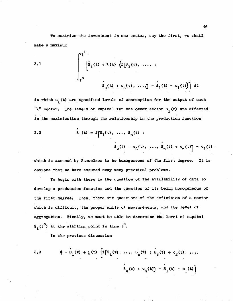
46To maximize the investment in one sector, say the first, we shall
make a maximum
"i" sector. The levels of capital for the other sector (t) are affected
in the maximization through the relationship in the production function
which is assumed by Samuelson to be homogeneous of the first degree. It is
obvious that we have assumed away many practical problems.
To begin with there is the question of the availability of data to
develop a production function and the question of its being homogeneous of
the first degree. Then, there are questions of the definition of a sector
which is difficult, the proper units of measurements, and the level of
aggregation. Finally, we must be able to determine the level of capital
S^(t°) at the starting point in time t°.
^ -J-11
3.1
in which c (-t) are specified levels of consumption for the output of each
3.2 • • • > S^(t) j
In the previous discussion
3.3 I • • • f Sn(t) j Sg(t) + c2(t), ...,
47
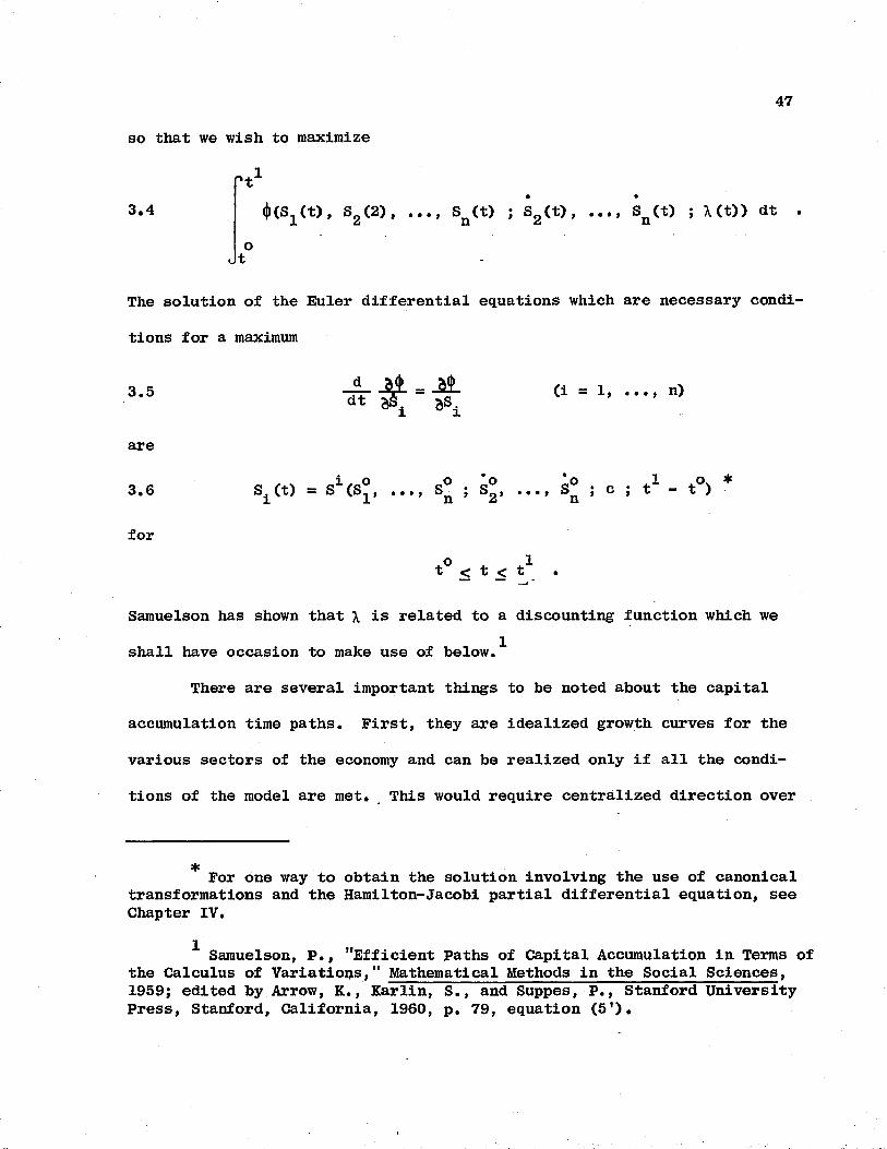
so that we wish to maximize
r't1
3.4 (j)(S1(t), S2(2), Sn (t) ; S2(t>, Sn (t) ; \(t)) dt .ot
The solution of the Euler differential equations which are necessary condi
tions for a maximum
3-5 = 0 = 1 ”)i 8s!
are
3.6 S;L(t) = S (Sr • • •, Sn ; Sg, • «•, ; c ; t — t )
foro 1t < t < t
Samuelson has shown that \ is related to a discounting function which we
shall have occasion to make use of below.^
There are several important things to be noted about the capital
accumulation time paths. First, they are idealized growth curves for the
various sectors of the economy and can be realized only if all the condi
tions of the model are met. This would require centralized direction over
j|( For one way to obtain the solution involving the use of canonical transformations and the Hamilton-Jaeobi partial differential equation, see Chapter IV.
1 Samuelson, P., "Efficient Paths of Capital Accumulation in Terms of the Calculus of Variations," Mathematical Methods in the Social Sciences, 1959; edited by Arrow, K., Karlin, S., and Suppes, P., Stanford University Press, Stanford, California, 1960, p. 79, equation (5').
48
the allocation of resources and realism in the economic relationships which
the equations describe. Realistically, they are goals or benchmarks against
which to measure actual growth in an investment plan. Second, while it is
only investment in the first sector which is maximized, all the investment
paths are efficient. However, for the sectors other than the first, the
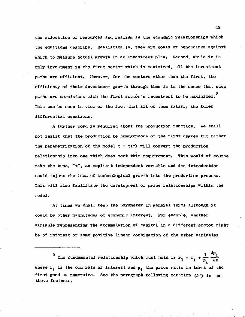
efficiency of their investment growth through time is in the sense that such2paths are consistent with the first sector’s investment to be maximized.
This can be seen in view of the fact that all of them satisfy the Euler
differential equations.
A further word is required about the production function. We shall
not insist that the production be homogeneous of the first degree but rather
the parametrization of the model t = t(T) will convert the production
relationship into one which does meet this requirement. This would of course
make the time, "t", an explicit independent variable and its introduction
could inject the idea of technological growth into the production process.
This will also facilitate the development of price relationships within the
model.
At times we shall keep the parameter in general terms although it
could be other magnitudes of economic interest. For example, another
variable representing the accumulation of capital in a different sector might
be of interest or some positive linear combination of the other variables
where r^ is the own rate of interest and p^ the price ratio in terms of thefirst good as numeraire. See the paragraph following equation (5 1) in the above footnote.
2 The fundamental relationship which must hold is r. = r^ + P± dt
might be used. In particular the latter could be the square root of the
sum of squares of the other variables which would from a mathematical point
of view make the variable of integration an arc length, while from an
economic standpoint the levels of capital accumulation would be in terms of
such a metric. Of course, we retain the flexibility of keeping the variables
as functions of time. Finally, regardless of the parametrization relative
prices remain the same which, of course, is what is required, for we do not
wish the basic structural relationships to be affected by the change in the
mathematical representation.
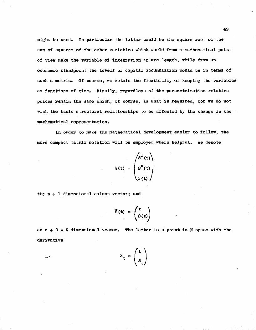
In order to make the mathematical development easier to follow, the
more compact matrix notation will be employed where helpful. We denote
an n + 2 = N dimensional vector. The latter is a point in N space with the
derivative
the n + 1 dimensional column vector; and
503which we assume to be continuous. Where there are no superscripts the
subscripts denote differentation of the matrix or vector in the usual
manner. Then the right hand side of 3.3 can be represented as <J>£(S(t) ;
St (t)], a continuous function of the 2n + 1 elements X,Sl ,S^ (i,j = 1, ..., n)where the c^ are stipulated and hence not variables. We shall sometimes
denote X(t) = Sn+*(t) where matrix notation is used. The derivative of <|>
with respect to the (n + 1)X1 column matrix S , <j> is a IX(n + 1) rowt
matrix p = (p., p _) known in the literature as the momentum matrix.1 n+1For the parametric case we shall use P = (P., ..., P „) = d> . Analogously,x n+^ gthe derivative of (j» with respect to the (n + 1)X1 column matrix S(t),(j»g is a IX(n + 1) row matrix (<|>sl, •••» <J>g n + 1). The Euler equations which must
be solved (see Chapter IV) to get the paths of maximum capital accumulation
can be written
3-7 It V = +8 •w
B. ECONOMIC ANALYSIS IN HIGHER DIMENSIONAL SPACE
It is obvious that if an analysis can take into account more variables
or factors which affect a particular activity, more information will be
obtained and more insight gained. The nature of efficient paths of capital
accumulation is no exception. However, it is not always appreciated that
additional information may be obtained by carrying out the analysis in a
3 The full use of matrix notation in the Calculus of Variations hasbeen made by Murnaghan, F., "The Calculus of Variations," Lectures on AppliedMathematics," issued by the David Taylor Model Basin, Washington, D.C. Thishas also appeared under the same title as a book published by the Spartan Press, Washington, D.C.
51higher dimensional space to get at the full implications of the relation
ships to be studied. This means that full advantage is not taken of all
the information that is embedded in a given set of relationships. We shall
take advantage of the opportunity to do this in utilizing the Calculus of
Variations as the tool of economic analysis.
1. Role of Constraints
The question arises as to whether restraints on paths of capital
accumulation can be revealed in working in a higher dimensional space which
otherwise would not be evident? The answer is, of course, affirmative and
we shall not only exhibit such relationships but, also, demonstrate the
utility of this approach for economic analysis. Moreover, by parameterizing
the relationships we shall be able to reveal a spectrum of economic implica
tions including constraints to which capital growth is subject.
As indicated previously, we shall make time a function of T which
will, in turn, make the stock of capital and capital formation functions of t.
Of course we can specialize t = t. Secondly, we shall work with the
Hamiltonian function
n+23.8 H(S,p) = £ p± S* - <j>(S,St)
i=l
which is defined in the 2N space (S,P) in which we shall carry out the
analysis. It will be shown that the paths of capital accumulation will lie
on a 2N - 1 dimensional locus represented by K(S,P) = 0. Finally, we shall
cover the case where time is considered along with the stocks as one of the
explicitly stipulated variables as well as the conservative situation in
which it is not explicitly represented.
52
It is well known that in order to have a different variable of
integration give the same value of the integral we wish to maximize
f(S,S ) dtJa
it is necessary that the function
3.9 f(S(t) ; S <T)) = <Ks(t) ; s.(t)) t
be homogeneous of the first degree wich we shall assume. Thus we have in
abbreviated form' which we shall use hereafter except where confusion may
arise
3.10•eF dr =
a(|> dt
a
with the limits of integration changed accordingly. We may write the con
strained integrand as F t K with j* as a Lagrangian multiplier. In this
formulation, the coordinates of the space are the S and P referred to in
the literature as the extended phase space. In this space K is known as
the extended Hamiltonian function. It will be possible to consider three
specializations of this model:
It is well known that the integrand must be homogeneous of the first degree if.the integral is not to be affected by the parametrization. For a discussion of this question in the Calculus of Variations see Bliss, G., Lectures on the Calculus of Variations, The University of Chicago Press, Chicago, Illinois, 1946, Chapter V.
53
(1) The parametric integrand is conservative and K is specialized
to K = Pj + H(S,p) = 0. This as a conservative system is similar to the
current Samuelson model although he does not take specific advantage of this
relationship. However, we shall make use of it as the constraint which
operates in the 2N space.
(2) The parametric variable of integration is taken to be t = t
where t is an explicit variable. This will set jj = 1 so that the parametric
integrand is F + K.
(3) K = P^ + H(S,p) with t an explicit variable; thus, like (2)
above, the model is non-conservative. As a consequence H> the ordinary
Hamiltonian, is itself a function of the explicit variable t.
2. Current Capital Model Considered in this Space
Looked at in terms of the higher dimensional space, the Samuelson
model of capital accumulation presents an especially interesting aspect. To
begin with by assuming that the production function is homogeneous of the
first degreen
3.11 V * : Si « fL s1 ti=2 St
the integrand of the integral to be maximized
0 = S*(t) + xct) jf(S ; S^(t), ..., s” (t)) - S*(t) j
ghas the same property. This means that
Since consumption is stipulated and is therefore not a variable we shall omit it from the equations for the sake of convenience.
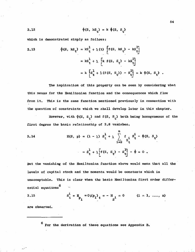
54
3.12 <j>(S, kSt) = k <J>(S, St)
which is demonstrated simply as follows:
3.13 (j»(S, kSt) = kS* + \(t) jf(S, kSt) - ksJJ
= ks* + \ jk f(s, st) - ksg
= k jsj + X(f(S, St)) - sJJ = k <|>(S, St) .
The implication of this property can be seen by considering what
this means for the Hamiltonian function and the consequences which flow
from it. This is the same function mentioned previously in connection with
the question of constraints which we shall develop later in this chapter.
However, with d>(S, S ) and f(S, S ) both being homogeneous of theX Xfirst degree the basic relationship of 3.8 vanishes.
n3.14 H(S, p) = (1 - \) + x Y f i st " ^ (S’ V
i=2 St
- * x[i<S, st) - s£j - 4 = 0
But the vanishing of the Hamiltonian function above would mean that all the
levels of capital stock and the momenta would be constants which is
unacceptable. This is clear when the basic Hamiltonian first order differ- 6ential equations
3.15 S* = H = 0 ;(p ) = - H = 0 (i = 1, ..., n)* pi i.t s1
are observed.
6 For the derivation of these equations see Appendix B.
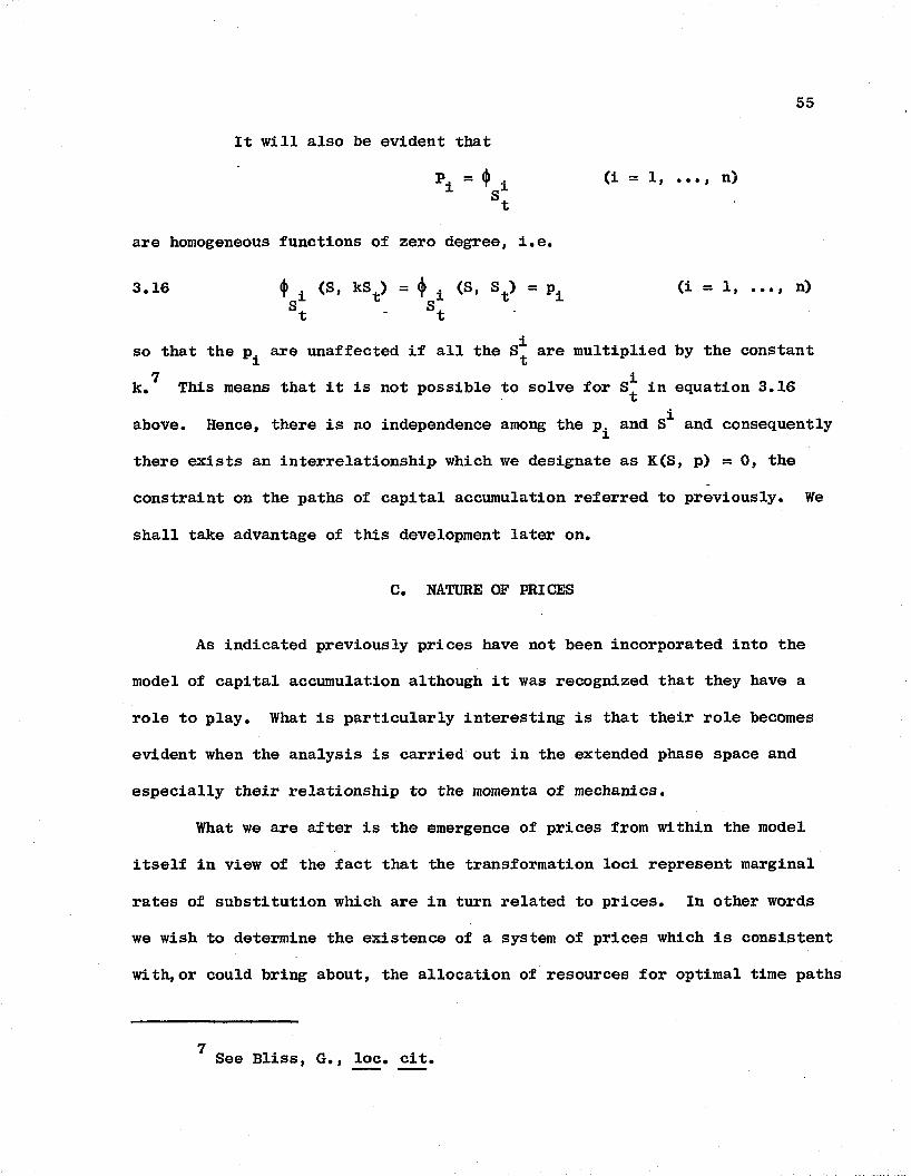
It will also be evident that
P = ()• j (i = 1, ..., n)st
are homogeneous functions of zero degree, i.e.
3.16 <|» ± <S, kS+) = <|> ± (S, St) = p± (i = 1, ..., n)
so that the are unaffected if all the S* are multiplied by the constant7 ik. This means that it is not possible to solve for in equation 3.16
above. Hence, there is no independence among the p^ and S* and consequently
there exists an interrelationship which we designate as K(S, p) = 0, the
constraint on the paths of capital accumulation referred to previously. We
shall take advantage of this development later on.
C. NATURE OF PRICES
As indicated previously prices have not been incorporated into the
model of capital accumulation although it was recognized that they have a
role to play. What is particularly interesting is that their role becomes
evident when the analysis is carried out in the extended phase space and
especially their relationship to the momenta of mechanics.
What we are after is the emergence of prices from within the model
itself in view of the fact that the transformation loci represent marginal
rates of substitution which are in turn related to prices. In other words
we wish to determine the existence of a system of prices which is consistent
with, or could bring about, the allocation of resources for optimal time paths
7 See Bliss, G., loc. cit.
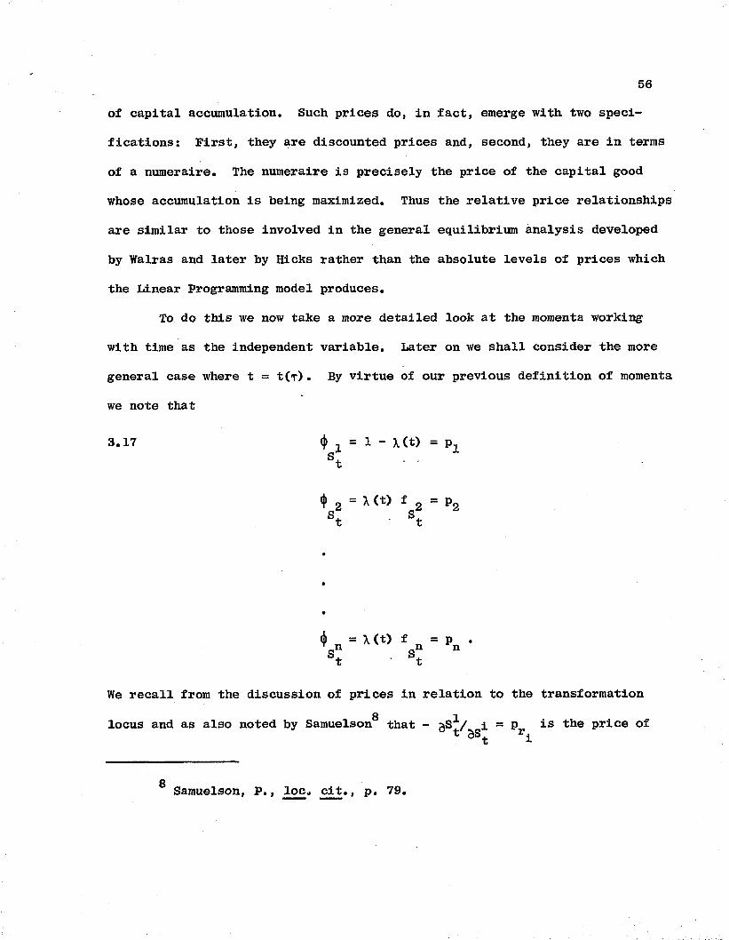
of capital accumulation. Such prices do, in fact, emerge with two speci
fications: First, they are discounted prices and, second, they are in terms
of a numeraire. The numeraire is precisely the price of the capital good
whose accumulation is being maximized. Thus the relative price relationships
are similar to those involved in the general equilibrium analysis developed
by Walras and later by Hicks rather than the absolute levels of prices which
the Linear Programming model produces.
To do this we now take a more detailed look at the momenta working
with time as the independent variable. Later on we shall consider the more
general case where t = t(T). By virtue of our previous definition of momenta
we note that
3.17 <(> 1 = 1 - \(t) = px
<j> = \(t) f = p .sn sn nt * t
We recall from the discussion of prices in relation to the transformation8 1locus and as also noted by Samuelson that - gS"y i = P is the price oft 3St i
g Samuelson, P., loc. cit., p. 79.
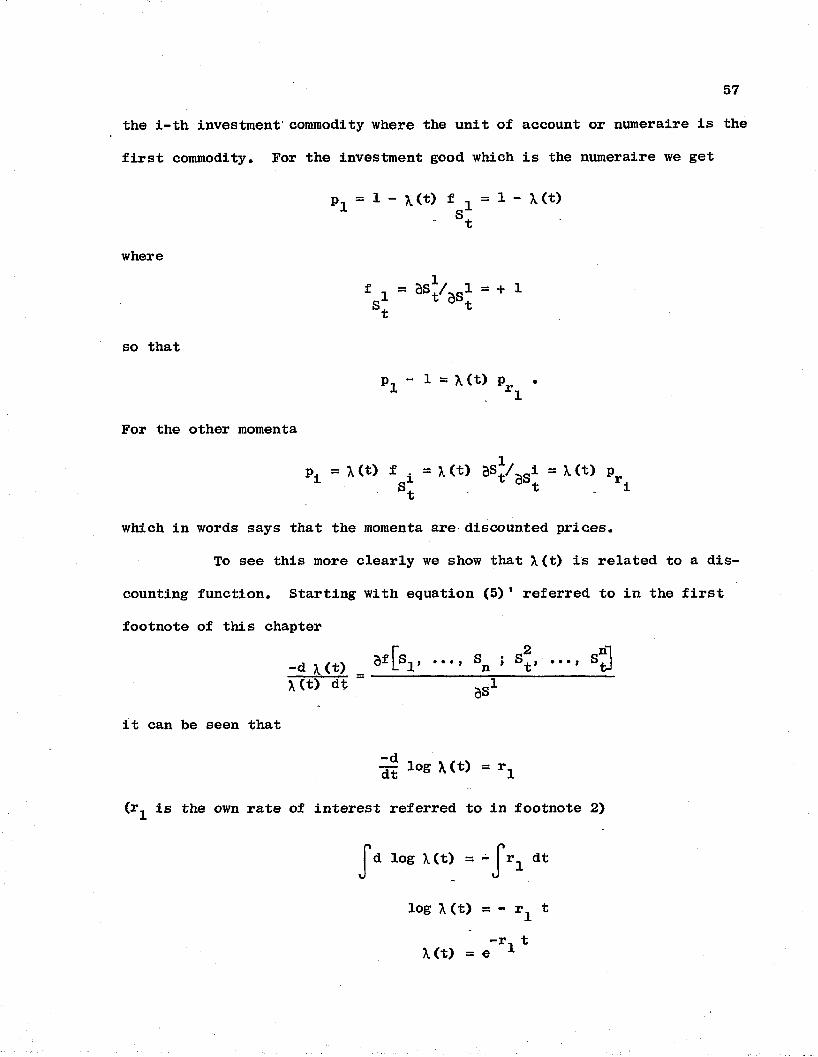
57
the i-th investment' commodity where the unit of account or numeraire is the
first commodity. For the investment good which is the numeraire we get
P, = 1 - \<t) f i = 1 - \<t) st
where
so that
Px - 1 = x(t) Pr .
For the other momenta
P, = X (t) f . = \ (t) as*/ i = \ (t) p S 1 t ast r.X
which in words says that the momenta are discounted prices.
To see this more clearly we show that X(t) is related to a dis
counting function. Starting with equation (5)' referred to in the first
footnote of this chapter
-d x(t) = af[s2> sn ; s;,..., sgX(t) dt BS1
it can be seen that
^ l o g \ ( t ) = r 1
is the own rate of interest referred to in footnote 2)
d log X(t) = - I r. dt
log X(t) = - rJL t-r t
X(t) = e 1
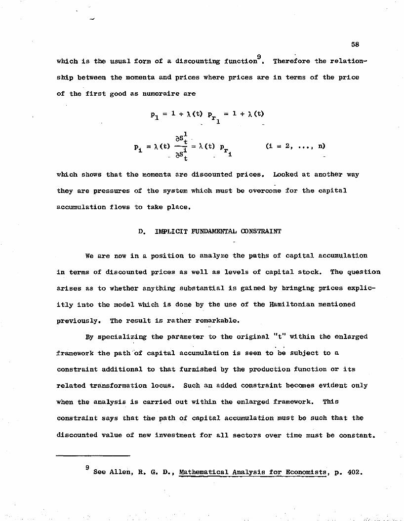
58gwhich is the usual form of a discounting function . Therefore the relation
ship between the momenta and prices where prices are in terms of the price
of the first good as numeraire are
P, = 1 + X(t) p = 1 + X(t). 1
as IP. = X (t) — T = X (t) p (i = 2, ..., n)
3s ; - 1
which shows that the momenta are discounted prices. Looked at another way
they are pressures of the system which must be overcome for the capital
accumulation flows to take place.
D. IMPLICIT FUNDAMENTAL CONSTRAINT
We are now in a position to analyze the paths of capital accumulation
in terms of discounted prices as well as levels of capital stock. The question
arises as to whether anything substantial is gained by bringing prices explic
itly into the model which is done by the use of the Hamiltonian mentioned
previously. The result is rather remarkable.
By specializing the parameter to the original "t" within the enlarged
framework the path of capital accumulation is seen to be subject to a
constraint additional to that furnished by the production function or its
related transformation locus. Such an added constraint becomes evident only
when the analysis is carried out within the enlarged framework. This
constraint says that the path of capital accumulation must be such that the
discounted value of new investment for all sectors over time must be constant.
g See Allen, R. G. D., Mathematical Analysis for Economists, p. 402.
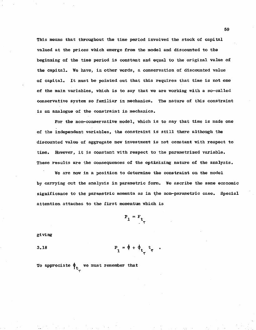
59
This means that throughout the time period involved the stock of capital
valued at the prices which emerge from the model and discounted to the
beginning of the time period is constant and equal to the original value of
the capital. We have, in other words, a conservation of discounted value
of capital. It must be pointed out that this requires that time is not one
of the main variables, which is to say that we are working with a so-called
conservative system so familiar in mechanics. The nature of this constraint
is an analogue of the constraint in mechanics.
For the non-conservative model, which is to say that time is made one
of the independent variables, the constraint is still there although the
discounted value of aggregate new investment is not constant with respect to
time. However, it is constant with respect to the parametrized variable.
These results are the consequences of the optimizing nature of the analysis.
We are now in a position to determine the constraint on the model
by carrying out the analysis in parametric form. We ascribe the same economic
significance to the parametric momenta as in t)ae non-parametric case. Special
attention attaches to the first momentum which is
. T
giving
3.18 P = <j) + d> t1 V T
To appreciate (|>t we must remember thatT
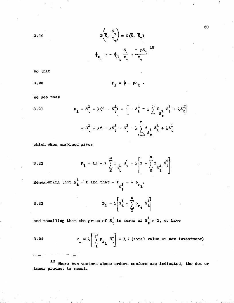
603.19
so that
3.20
We see that
3.21
♦ Is . - r - t<s . S J
S - pS, 10
t T T
Pj = ♦ - PBt •
= sj + X(f - sJ) + r - a\ - X £ i s* + xsjjt
n= s* + M - xsj - a\ - x £ fB± s* + Xs*
which when combined gives
i=2 St
3.22n
px - w - x l ± , a* -2 St
= Xn
-I v s t2 t
Remembering that S = f and that - f . = + p ,* s~ ri
v
3.23 P l - Xn
and recalling that the price of S* in terms of = 1, we havev v
3.24 P2 = Xn
IL 1P S pr. t x
= \ • (total value of new investment)
Where two vectors whose orders conform are indicated, the dot or inner product is meant.
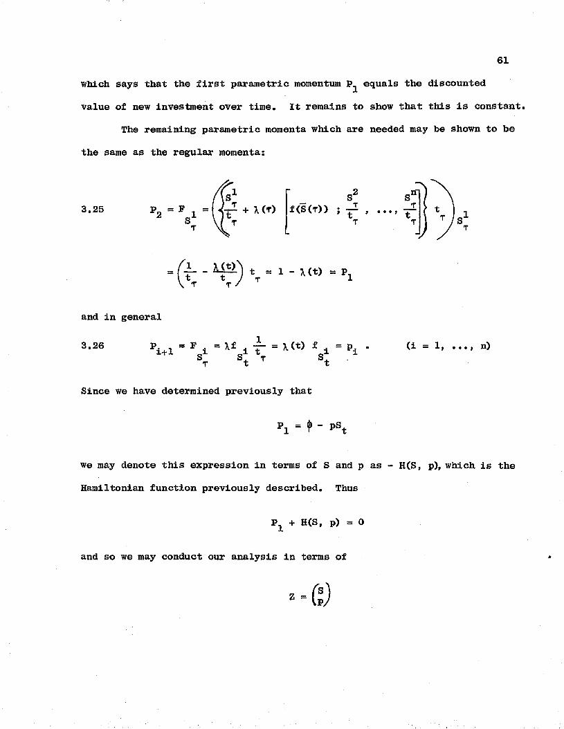
which says that the first parametric momentum P^ equals the discounted
value of new investment over time. It remains to show that this is constant.
The remaining parametric momenta which are needed may be shown to be
the same as the regular momenta:
3.25 + H t)
and in general
3.26 ?i 1 = p i = X f i — = \<t) f+ s* s\ \ s\
(i — 1) • • • t n)
Since we have determined previously that
we may denote this expression in terms of S and p as - H(S, p), which is the
Hamiltonian function previously described. Thus
Px + H(S, p) = 0
and so we may conduct our analysis in terms of
62
which is the extended phase space mentioned above. This means that the paths
of capital accumulation in this space must be on a 2N - 1 dimensional locus
Y(Z) = P^ + H(S, p) = 0 . If our model is conservative, which means that
time is not an explicit independent variable, then H(S, p), the Hamiltonian,
will not be a function of time. Therefore, = 0 so that H(S, p) is constant
through time. But the Hamiltonian is the discounted value of new investment.
This means, from a geometric point of view, that the paths of capital accumu
lation must lie on a constant discounted investment plane.
Since we are working with the Hamiltonian to describe the 2N - 1 locus
on which the paths of capital accumulation must lie, this is an appropriate
place to state some results which will be used later on. The Hamilton first
order partial differential equations 2N in number (contrasted with the N
Euler second order differential equations) which are derived in the appendix,
are
Pt = H«Hg
S T = - •
The first equation in the last block of N equations is particularly revealing:
3.27 tT = n'FP1 .
If the constraint isP1 = H(S, p) = 0 ,
then
3.28 t = jj, ,
and if we select t « t then jj, = 1, thus demonstrating B.l.(2) above. The
This is the economic counterpart of the constant energy level inmechanics.
advantages of working with the Hamilton canonical equations rather than the
Euler equations have to do with the method of obtaining solutions covered
in the following chapter.
E. EFFICIENT PATHS IN N SPACE AND IN THE EXTENDED PHASE SPACE
We again make use of the relationship between the space in which S
and S are the variables and the space in which S and P are the variablesb
(j)(S, St) = PSt - H(S, p)
12which holds for all trajectories whether or not they are extremals. By
differentiating both sides with respect to p we see that
3.29 S = Ht P
for any smooth cure in the N dimensional time coordinate space. This is a
different way of defining the momentum matrix p rather than identifying a
particular smooth trajectory. Any such curve can be embedded in the 2N
dimensional extended phase space where S and P are functions of the general
variable t defined in the interval a T < (3 • In this larger space the
integrand to be considered is
which follows from the fact that F is a positively homogeneous function of
the first degree. The paths of capital accumulation in this space are
constrained to be in the 2N - 1 dimensional locus K(S, P) which we have
12 The integral of the right-hand number is sometimes referred to as the canonical integral. See Lanczos, C., loc. cit., p. 168.
64
specialized to P. + H(S, p) = y = 0 . This constraint we have observed in
3.17 is the discounted value of new investment which is constant at all
times of the period under investigation.
It would appear, therefore, that the proper method of analysis is to
maximize the level of capital accumulation subject to both the production
constraint and to the constraint for which the discounted value of new
investment is constant. This would involve information regarding relative
prices which would double the data problem for planners. However, the
optimal or efficient paths obtained when the additional constraint is imposed
and relative prices are used is precisely the efficient path which results
from the optimization when this constraint and relative prices are not part
of the model.
This would add a great deal of flexibility to a planning operation.
Carrying out the analysis and plans without relative prices as inputs presents
a much lighter computation burden. In fact, only half as many equations must
be solved. On the other hand, it may be more feasible to monitor relative
prices in the economy as a means of determining whether investments are pro
ceeding in line with plans. Moreover, there may be reasons why it would be
desirable to know the magnitude and structure of relative prices particularly
in regard to the basic resources available to the economy and the way in
which soceity determines such values.
We shall now demonstrate this result. Utilizing this form of the
constraint and t = t, by virtue of the previous analysis involving the
Hamiltonian differential equations, t =1; the Jjagrangian multiplier u, = 1.T
Hence, S = y along the image in the 2N space of any smooth curve in the N t O
65
dimensional time coordinate space. But this is the first N differential
equations which arise from the determination of an extremal curve of a
constrained problem in the 2N dimensional framework of analysis in which
the variables are S and P. We now investigate what will satisfy the other
N equations
3.31 P = - fcT
which become by virtue of our specialization
3.32 Pt = - Ys = - Ks .
These equations are satisfied if, and only if, the paths of capital accumu
lation which are mapped into the S,P framework of analysis are themselves
extremal paths of an unconstrained maximization of <j>(S, ST) . This may be
seen by noting that the Euler equation for the unconstrained problem is
P = F T swhich, beeause^F = (j»t , may be written as
3.33 Ptt = fs
or
pt = *s •
However, on differentiating our previously used relation (j)(S, S^) = pSt - H(S , p)
with respect to S (S being held fixed) givesT
3.34 +S = 4 ' HS - H T PS •PTSince S = H or S = H , by substituting in the above equation we obtain
p ' pT<!>„ = — H which then yields the desired result ^
66
3.35 Pt H,SThus, we have the result that extremal paths of the unconstrained maximiza- ,
tion when considered within the framework of capital stocks, S(t), are,
when analyzed in the higher dimensional space of S(t) and P(t), the extremal
paths where the constraint P(t) + H(S, p) = 0 exists.
By carrying out the analysis within this level of generality we can
more easily see the impact of our assumptions about the relationships
governing the capital structure. If the relationships are conservative,
i.e. time has not been set up as an explicit variable, then the first of the
second N differential equations
because the Hamiltonian function is not a function of t .
On the other hand if t is made an explicit variable, then the
Hamiltonian is a function of t so that
which shows the time path of the discounted value of total new investment.
This means that, unlike the conservative case covered above, the paths of
capital accumulation do not lie on the plane which represents the constant
discounted value of new investments. This can be understood to mean that
at any point in time the original discounted value of the stock of capital
is not constant. The prices used are those which arise from the model.
(pi \ = - Ht<s’ p) - 0
3.36
<67
P. TRANSVERSAL SURFACES AND THE ENVELOPE13
The purpose of this section is to clarify and put in its proper
setting the current view of the role of the transversality conditions in a
capital model. The idea that there is a locus of possible points on which
the stock of capital of the first sector, for example, may lie is at the
heart of the concept of the transformation locus which has been central to
our analysis in this chapter. Each of the points on the transformation
locus represents differing levels of the capital stock S1 and the other
(n - 1) capital stocks. Since there are the technologically determined
possibilities, they also represent the constraint on the maximization of
the stock of capital in the first sector.
Following Samuelson, we assume that S1 achieves its maximum at the
terminal point
3.37 S1(t1) = E U t 1) ; SCt1), ..., ; S1(t°), ..., sn (t°)) ,
but in keeping with the literature of the Calculus of Variations this
function is called the transversal surface. This is done to distinguish
the case of a transversal surface from that of an envelope function. In
the former case an efficient path of capital accumulation would pierce the
locus, while in the latter case it would be tangent at its maximum point.
The object here is to show that the same price relationships hold for14capital stocks and new investment.
13 The transformation locus is used both for transversality and as an envelope. We shall distinguish both uses.
14 Samuelson, P. A., loc. cit.
68
To accomplish this we shall make use of one of the well known results
of the Calculus of Variations which says that for an efficient or extremal
path and a given transversal locus L(S) = 0, the following relationship holds
Lg(S) = P
where P is the vector of momenta previously considered. By taking
L(S) = E ,we have
3.38 L , = P. =p. = f = pS 1+1 1 S1 ri
If we set X = 1j we then have1 las as
3.39 = pi i ras ast i
15which is the result obtained by Samuelson, but more directly.
The transversality requirements, however, can be considered from a
different point of view. The locus of possible positions which the S1 may
assume at the terminal point in time is S1 = 01 (t) . We now state another
version of the transversality conditions as
n 4 j3.40 9 + £ (8t - St) 9 i = 0
i=l ' St
which can be written as
t - £ ■ i t .i=l St St
15 Ibid
69
However, by virtue of the homogeneity condition
♦ - y s t t * = °i=i st
so thatn
which shows that transversality is a generalization of orthogonality.
To understand the use of the transformation locus L or E as an
envelope it is necessary to go to Samuelson’s discussion of the discrete
treatment of capital in Chapter 12 of Linear Programming and Economic
Analysis." There for the intermediate time periods the envelope is tangent
to a series of alternative levels of capital accumulation, each proceeding*from differing levels of capital in the previous time period. (See
Figure 12-1 of Chapter 12). Once the point of tangency has been determined
then the efficient path is that which will pierce the locus at that point.
G. ECONOMIC SIGNIFICANCE OF THE ANALYSIS
Any model has the potential to be useful in at least either of two
ways: to derive theoretical results not otherwise readily obtainable, or
as a means for arriving at economic policy decisions. The expanded model
considered in this study belongs to the former category although with further
development there is some hope of ultimately being useful in the area of
economic planning and decision-making. What has been demonstrated is the
usefulness of applying the Hamilton-Jacobi formulation of the Calculus of
Variations in analyzing the implications of a capital model under varying
70
assumptions. This has been done by obtaining some new results as well as
results which are consistent with results obtained with other types of models.
Although the focus of attention has been on a capital model, it is clear that
the Hamilton-Jacobi formulation also could be applied to other models either
on an aggregate or multi-sectored level in which utilities, consumption, or
other economic activities could be maximized with or without constraints.
We are now able to draw a somewhat sharper distinction between the
capital model and the aggregate models, e.g. Harrod-Domar, described in the
first part of Chapter II. Not only is there the distinction between an
aggregate and a multi-sector model but also the matter of constraints operating
within the system. The idea that the activity of a particular sector has an
impact on many other sectors and may be limited by such sectors is by now
well recognized. The input-output model and its incorporation into a Linear
Programming formulation described briefly in the latter part of Chapter II
represents a discrete model in which resource restraints are imposed. However,
neither the Harrod-Domar model nor the Hicks-Samuelson model could be used
to analyze growth of an industry or sector because there are no resource
constraints incorporated into the analysis. The capital model developed in
this chapter in addition to having constraints represents a continuous version
and is an alternative to the discrete model mentioned above.
In the continuous capital model we have investigated, the role of time
becomes of great interest. It has been shown that previous capital models
have been time independent, which means that technology is constant in the
sense that it does not affect the production function. It has been shown
that such a limitation can be removed as long as the new production function
is homogeneous of the first order. This means that the impact of changes in
71
technology on the production function can be Incorporated into the model.
This opens up the possibility of developing more dynamic models in which
changes through time are explicitly taken into account.
The potential usefulness of the Hamilton-Jacobi formulation in
theoretical economic analysis is more obvious when the model can be spe
cialized to produce results which agree with results from other methods of
approach. It has been shown that given a conservative or time independent
model there exist a discount rate, an own rate of interest and a set of
technologically determined price ratios which appear in the form of a
constraint that the discounted value of all new investment is a constant.
This is comparable to the well known result that an accumulated value of a
constant stream at a given rate in a specified time period is the discounted
present value itself growing at that fixed rate of interest. It is worthy
of note that this appears 'as a constraint when time is not explicitly a part
of the model but when time is included the result is not obtained. We have
something very similar to the Von Neumann result that the maximum rate of
growth and the interest rate are equal for multi-sector models. It should
be noted, moreover, that the existence of such prices, discount rates and
own rates of interest or growth rates does not imply that they reflect actual
market conditions. Rather, they represent a set of consistent relationships
derived from the model itself.
One of the especially interesting results obtained, that the path of
maximum investment is independent of prices, requires a word of comment.
From a mathematical standpoint this is one of the remarkable results of the
Hamilton-Jacobi formulation of the Calculus of Variations. The result is
perhaps a little less surprising from an economic standpoint in view of the
fact that the prices inherent in the model are assumed to be technologically
determined by the transformation locus. Once the result is obtained it
becomes almost obvious since in this type of model such prices are inherent
in the maximizing relationships. The fact that the powerful tools of the
Calculus of Variations can produce results which are recognizable and
acceptable and frequently made more easily understood serve to enhance its
usefulness as a sophisticated means of economic analysis.
CHAPTER IV
IMPLICATIONS OF COMPUTATIONAL METHODS FOR ECONOMIC ANALYSIS
A. AN OVERALL VIEW
It has been recognized for a long time that the usefulness of
methods of economic analysis is not limited to those which can produce
numerical results. Purely theoretical results in both the micro and macro
economic fields have been obtained using very general functional relation
ships in the ordinary calculus as has been shown in the first chapter. It
is the purpose of this chapter, however, to show not only the various ways
in which numerical results can be obtained for a capital model but, also,
the economic content of these procedures. The discussion, however, will
not be concerned with the detailed mathematics of the numerical analysis
but rather the conceptual framework within which the analysis takes place.
The maximum usefulness of a capital model in economic analysis and
policy formulation requires both the proper logical relationships and,
also, the ability to determine economic magnitudes. This added dimension
to the content of economic analysis has been enhanced and spurred on by
the advent of the general purpose electronic digital computer and the
related field of Operations Research during the past decade. This expanded
capability extends to the area of the Calculus of Variations and has, in
turn, spurred on renewed interest in the development of more efficient
analytical and numerical methods for solving such problems. It should be
of considerable interest, therefore, to the economics profession to be
aware of those areas where further mathematical results could have
74
important implications for the further development of economic models
generally and a capital model in particular.
B. METHODS OF SOLUTION
The basic problem of obtaining efficient paths of capital accumula
tion involves the solution of the Euler second order differential equations
in which there are generally conditions to be met at both the initial and
terminal points. However, as indicated previously, for many problems it
makes more sense to consider either or both the initial and terminal values
lying on some locus or loci of possible values and to determine the most
efficient paths under such circumstances. In terms of a capital model, the
prescribed initial conditions represent the levels of investment in each of
the capital sectors at the beginning of the economic process under investi
gation, while the terminal conditions if they are specified, are the levels
of investment at some future time. It is obvious that a general solution
will give the levels of capital goods at all the intermediate time periods.
There are two principal methods of obtaining the solution or tra
jectories of capital accumulation: (1) by the use of generating functions,
and (2) by what is referred to in the literature as "direct methods." The
latter is a more recent development and seems more directly oriented to a
computer solution. The use of generating functions also is dependent to
a considerable extent on a computer solution except for very special cases
where so-called analytical solutions may be obtained.
7511. Use of Generating Functions
It is of very considerable interest that the use of generating
functions to get solutions requires the differential equations to be in
the Hamilton canonical form, and serves as a strong motivation for carrying
out the analysis in this higher dimensional space. This means that in this
larger space with s^ and p^ (i = 1, . N) as the coordinates both the
levels of capital accumulation and the price related momenta must be taken
into account. Essentially, what is wanted is some transformation of the
s^ and p^ into another coordinate system which will preserve the canonical
character of the model and, at the same time, make the integration of the
set of first order differential equations easier to solve. Here, too, it
is possible to handle a capital model in which time is not explicitly
stipulated as well as the time dependent case.
a. Hamilton's Principle Function
The nature of Hamilton's principle function can be intro
duced by the use of geometrical concepts. What is wanted is a yardstick
or numeraire such that
— pb4.1 W(S, S) = J <j>(S, St) dt
An extensive discussion of the use of generating functions and the Hamilton-Jacobi partial differential equation can be found in Lanczos, C., The Variational Principles of Mechanics, University of Toronto Press, Toronto. See especially Chapters VII and VIII. See also Akhiezer, N. I., The Calculus of Variations; Gelfand, I. M, and Fomin, S.V., Calculus of Variations; and Elsgolc, L. E., Calculus of Variations; all recent translations from Russian.
76
has the value of the length of S expressed in the coordinates of the two
points S and S. Such paths for the time independent case which we consider
first are known as geodesics or shortest lines in the appropriate space.2The use of different metrics or numeraires is not uncommon in the develop
ment of economic theory. Walras, in his theory of general equilibrium,
Elements d^conomic Politique Pure, gave prominent place to the selection3 'of a proper numeraire. The challenge here, however, is to be able to find
a metric which has useful economic content and at the same time will give
the length of the curve S as the value of the integral.
The value of this function lies in the fact that the solu
tion of the paths can be obtained by differentiation and elimination rather
than integration. Thus we can obtain
4.2 p± = Wg (S, S)
i, = <8, S)To obtain S.(t) let us assume that i
ws s sisj* 0
2 In many applications it is helpful to use the arc length as a metric. For the case where G is a matrix and dx a vector of differentials, the metric is (dx^Gdx)® which is known as a metric in Riemannian space.If the function defining the metric obeys other mild conditions the space is called a Finsler space. For an illuminating discussion of the relationship of Finsler spaces to the Calculus of Variations see Rund, H., The Differential Geometry of Finsler Spaces, Springer-Verlag, Berlin (1959) pp. 1-43.
3 A numeraire as used in economics is usually a one dimensional concept, a good used as a unit of accounting. Metric is generally an n dimensional concept. Viewed in this manner index numbers fall in this latter category.
so that
4.3 Si = sUs, p)
and substituting this in
P, = W (S, S)1 Si
gives
4.4 = p1(S, p)
where and p^ are the initial levels of capital stock and price related
momenta.
As has been shown previously, the paths of capital accumula
tion are constrained to lie, for the time independent case, on a 2N - 1
dimensional space where the Hamiltonian is equal to a constant. It can be
shown that the principle function of Hamilton, W(S, S) satisfies the
partial differential equation
4.5 H(S, W ) = E E = constantO
for any S. However, it also satisfies the initial points so that
4.6 H(S, - Wg) = E .
To approach the problem this way from a numerical standpoint is not very
helpful since the determination of W(S, S) has'to satisfy simultaneously
these two partial differential equations which is extremely difficult to
achieve.
We can handle the time dependent case in a straightforward
manner in accordance with our previous approach to this general problem.
The procedure is to consider time as an explicit variable in the extended
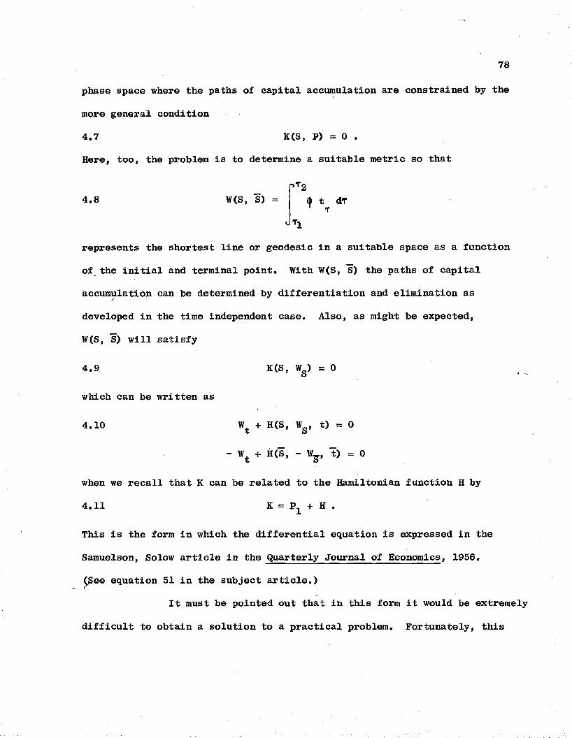
78
phase space where the paths of capital accumulation are constrained by the
more general condition
4.7 K(S, P) = 0 .
Here, too, the problem is to determine a suitable metric so that
r»Tr4.8 W(S, S) = ft drT
Jtxrepresents the shortest line or geodesic in a suitable space as a function
of the initial and terminal point. With W(S, S) the paths of capital
accumulation can be determined by differentiation and elimination as
developed in the time independent case. Also, as might be expected,
W(S, S) will satisfy
4.9 K(S, Wg) = 0
which can be written as
4.10 Wt + H(S, Wg, t) = 0
- Wt + H(S, - W-g, t) = 0
when we recall that K can be related to the Hamiltonian function H by
4.11 K = P]L + H .
This is the form in which the differential equation is expressed in the
Samuelson, Solow article in the Quarterly Journal of Economics, 1956.
£See equation 51 in the subject article.)
It must be pointed out that in this form it would be extremely
difficult to obtain a solution to a practical problem. Fortunately, this
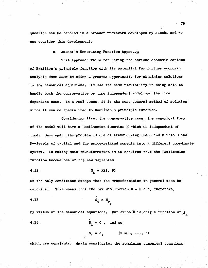
79
question can be handled in a broader framework developed by Jacobi and we
now consider this development.
b. Jacobi's Generating Function Approach
This approach while not having the obvious economic content
of Hamilton's principle function with its potential for further economic
analysis does seem to offer a greater opportunity for obtaining solutions
to the canonical equations. It has the same flexibility in being able to
handle both the conservative or time independent model and the time
dependent case. In a real sense, it is the more general method of solution
since it can be specialized to Hamilton's principle function.
Considering first the conservative case, the canonical form
of the model will have a Hamiltonian function H which is independent of
time. Once again the problem is one of transforming the S and P into S and
P— levels of capital and the price-related momenta into a different coordinate
system. In making this transformation it is required that the Hamiltonian
function become one of the new variables
4.12 S = H(S, P)n ’
as the only conditions except that the transformation in general must be
canonical. This means that the new Hamiltonian H = H and, therefore,
4.13 s± = Hi
by virtue of the canonical equations. But since H is only a function of snm
4.14 = 0 , and so
= d^ (i s 1, ..., n). r~
which are constants. Again considering the remaining canonical equations
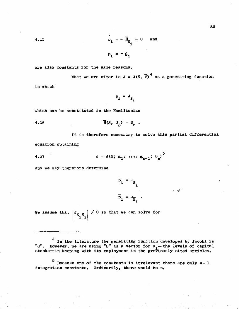
80
4.15 p = - H = 0 and 1 st
P, = - 8±
are also constants for the same reasons.4What we are after is J = J(S, S) as a generating function
in which
Pi = JSj
which can be substituted in the Hamiltonian
4.16 H<S, Js) = sn .
It is therefore necessary to solve this partial differential
equation obtaining5
4.17 J — J(S; •••»
and we may therefore determine
p = J i S.
We assume that S.S. i 3/ 0 so that we can solve for
4 In the literature the generating function developed by Jacobi is "S". However, we are using MS" as a vector for si— the levels of capital stocks— in keeping with its employment in the previously cited articles.
g Because one of the constants is irrelevant there are only n - 1 integration constants. Ordinarily, there would be n.
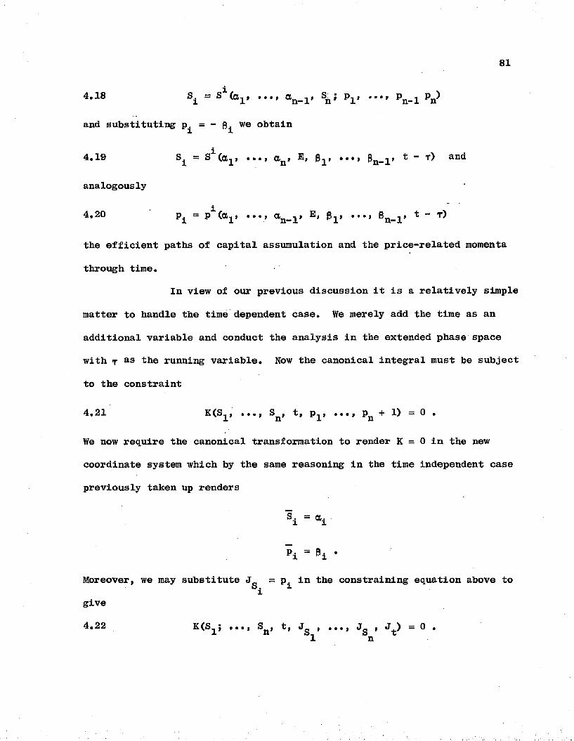
81
4.18 = S (a1> •••» P]_* •••» Pn_i
and substituting = - (3 we obtain
4.19 SA = S (otri •••> on » 3-j i •••> Pu—i’ t — t) and
analogously
4.20 p_ = p (og , •••> P]_* •••> Pn_2_» t - t)
the efficient paths of capital assumulation and the price-related momenta
through time.In view of our previous discussion it is a relatively simple
matter to handle the time dependent case. We merely add the time as an
additional variable and conduct the analysis in the extended phase space
with t as 'the running variable. Now the canonical integral must be subject
to the constraint
4.21 K(S^, «««, S^, t, •••» Pjj + 1) = 0 •
We now require the canonical transformation to render K = 0 in the new
coordinate system which by the same reasoning in the time independent case
previously taken up renders
s± = a*
pi = *i •Moreover, we may substitute J = p. in the constraining equation above to
Si 1give
4.22 K(S^j ..., Sn, t, Jg , ..., Jg , Jj_) = 0 .1 n
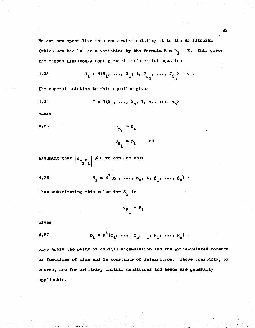
82
We can now specialize this constraint relating it to the Hamiltonian
(which now has "t" as a variable) by the formula K = P^ + H. This gives
the famous Hamilton-Jacobi partial differential equation
4.23 J + H(S^, iti, S^j tj Jg , «««, Jg ) = 0 .1 n
The general solution to this equation gives
4*24 J = J ( S • • • i Sn, t, CG-> •••» (ijj)
where
4.25 J = 0ai
assuming that Ja. S i i
Ja = P, aad Si i
/ 0 we can see that
4.26 S1 - S (ax» •••» CG i if P^f •••> 6n) •
Then substituting this value for in
JS = P 1 igives
4.27 p^ = p (<X-f •••f ttjjf •••t Pn) i
once again the paths of capital accumulation and the price-related momenta
as functions of time and 2n constants of integration. These constants, of
course, are for arbitrary initial conditions and hence are generally
applicable.
83
There axe many formal similarities between the use of
Hamilton's principle function and the generating function approach of 6Jacobi. The.use of Hamilton's principle function given the present state
of mathematical knowledge is not of practical value as a means of solving
problems. It offers considerable opportunity, however, for further
theoretical developments in economic analysis. Jacobi's transformation
approach does require the integration of the Hamilton-Jacobi partial
differential equation which is within the computing state-of-the-art.
Moreover, both the time independent and the time dependent models can be
handled, the former by a canonical transformation which changes the
Hamiltonian into one of the new variables, the latter by a transformation
which makes H = 0. Both these transformations are obtained by the solution
of the Hamilton-Jacobi partial differential equation.
2. Direct Methods
At the present time much attention is being given to the
development of direct methods of solution of variational problems no doubt
influenced by the advent of computers. Actually, many techniques fall
within this general framework and it is of some interest to note that
Russian mathematicians appear to be preeminent in this development. Only
the two most prominent methods, that of Euler's method of finite dif
ferences and the Ritz method similar to that of Kantorovic, will be
covered.
0For the deeper mathematical differences between Hamilton's
principle function and Jacobi's generating function see Lancos, C., op cit, pp. 254-264.
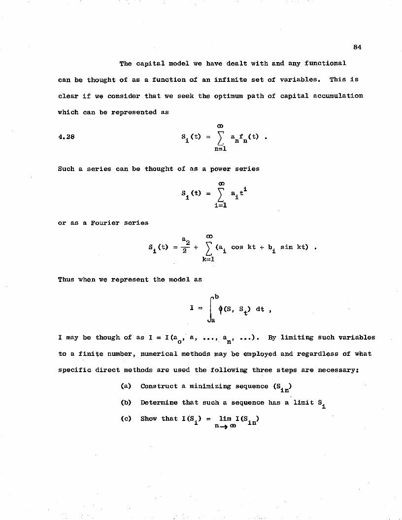
84
The capital model we have dealt with and any functional
can be thought of as a function of an infinite set of variables. This is
clear if we consider that we seek the optimum path of capital accumulation
which can be represented asoo
4.28 S, (t) = V a f (t) .i n nn='l
Such a series can be thought of as a power seriesOD
Si(t) = ^ a^t1i=l
or as a Fourier seriesooa 2(t) = -g— v V (a^ cos kt + b^ sin kt)
k=l
Thus when we represent the model as
i =Ja
f(S, S ) dt
I may be though of as I = I(aQ> a» •••» an > •••)• By limiting such variables
to a finite number, numerical methods may be employed and regardless of what
specific direct methods are used the following three steps are necessary:
(a) Construct a minimizing sequence (S^n)
(b) Determine that such a sequence has a limit
(c) Show that KS,) = lira I (S., )1 n_*GD ln
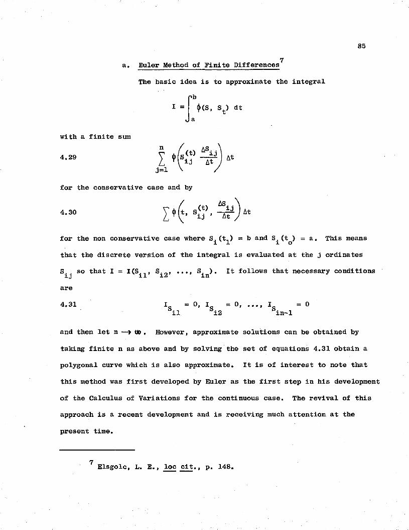
85 7a. Euler Method of Finite Differences
The basic idea is to approximate the integral ■»b
I = <|KSf st) dt
with a finite sum
4.29 £ ) At
for the conservative case and by
,(t) ^ij4.30 ^ ( t , S-',
for the non conservative case where = and = a * This means
that the discrete version of the integral is evaluated at the j ordinates
S,. so that I = I(SJ,f S . .... SJ ). It follows that necessary conditions ij ' il’ i2’ ’ inare
4.31 I = 0, I = 0, ..., I = 0il i2 in-1
and then let n — » Oo. However, approximate solutions can be obtained by
taking finite n as above and by solving the set of equations 4.31 obtain a
polygonal curve which is also approximate. It is of interest to note that
this method was first developed by Euler as the first step in his development
of the Calculus of Variations for the continuous case. The revival of this
approach is a recent development and is receiving much attention at the
present time.
7 Elsgolc, L. E., loc cit., p. 148.
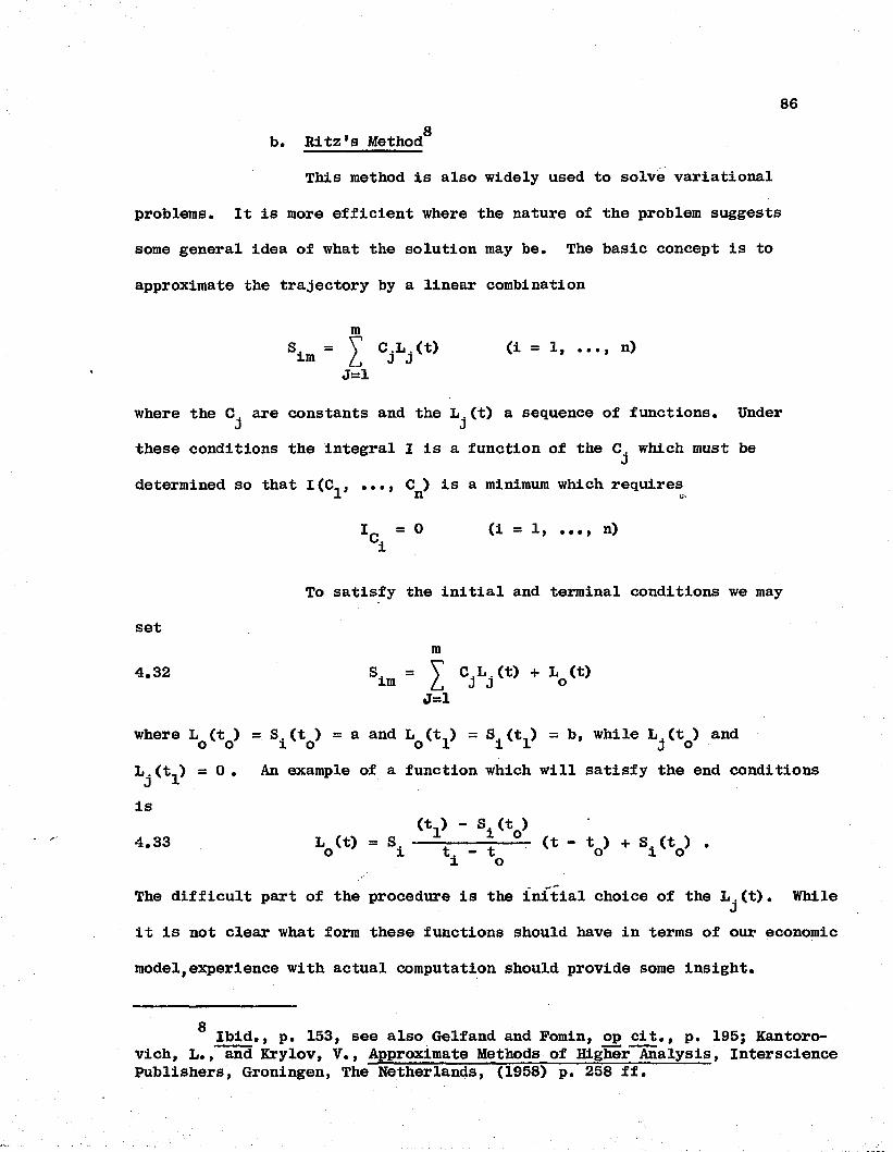
86g
b. Ritz's Method
This method is also widely used to solve variational
problems. It is more efficient where the nature of the problem suggests
some general idea of what the solution may be. The basic concept is to
approximate the trajectory by a linear combination
mS — y C.L.(t) (i — lt ..., n)
Zj “imJ=1
where the C. are constants and the L (t) a sequence of functions. Under J Jthese conditions the integral I is a function of the C which must be
•J
determined so that I(C., ..., C ) is a minimum which requires1 11 ij*
I = 0 (i = 1, ..., n)Ci
To satisfy the initial and terminal conditions we may
setm
4.32 Sln = £ CjLj (t) + Lo (t)J=1
where L (t ) =. S. (t ) = a and L (t.) = SJ(t,) = b, while L. (t ) and o o i o o l 1 1 j oL.(t.) = 0 . An example of a function which will satisfy the end conditions Jis
(t ) - S (t )4.33 L (t) = S4 --- -----=— — (t - t ) + S, (t ) .o i t . - t o i oi o
The difficult part of the procedure is the initial choice of the L . (t). While
it is not clear what form these functions should have in terms of our economic
model,experience with actual computation should provide some insight.
g Ibid., p. 153, see also Gelfand and Fomin, op cit., p. 195; Kantorovich, L., and Krylov, V., Approximate Methods of Higher Analysis, Interscience Publishers, Groningen, The Netherlands, (1958) p. 258 ff.

BIBLIOGRAPHY
SELECTED BIBLIOGRAPHY
A. ECONOMICS
Allen, R. G. D. Mathematical Analysis for Economists. London, 1938.In particular, Chapter 2CL
Bolza, Hans. "The Conception of Invariants in Dynamic Economics," Econometrica, Jan. 1936, Vol. 4, pp. 86-94.
Court, Louis M. "Entrepreneurial and Consumer Demand Theories for Commodity Spectra," Part I, Econometrica, April 1941, Vol. 9, pp. 135-162. Also see Part II, Econometrica, July-Oct. 1941, Vol. 9, pp. 241-297.
Creedy, F. "On Equations of Motion of Business Activity," Econometrica, Oct. 1934, Vol. 2, pp. 363-380.
_______ . "An Economic Interpretation of the Principle of Least Actionand Other Dynamical Theorems," Econometrica, Oct. 1935, Vol. 3, pp. 475.
Davis, Harold T. The Theory of Econometrics. The Principia Press.
_______ . "The Application of Functionals in Economics," (abs.),Econometrica, Oct. 1937, Vol. 5, pp. 384.
Evans, G. C. "A Simple Theory of Competition," American Mathematical Monthly, Vol. 29, 1922, pp. 371-380.
"Dynamics of Monopoly," American Mathematical Monthly, Vol. 31, 1924, pp. 77-83.
Mathematical Introduction to Economics. New York, 1930. In particular, Chapter 15 and Appendix II.
"Economics and the Calculus of Variations," Proceedings, National Academy of Science, Vol. 11, Jan. 1925.
. "The Mathematical Theory of Economics," American Mathematical Monthly, Vol. 32, March 1925. .
«vGeorgescu-Roegen, Nicholas. Discussion of "An Economic Interpretation of
the Principle of Least Action and Other Dynamical Theorems," (abs.), Econometrica, Oct. 1935, Vol. 3, pp. 475.
Hotelling, H. "A General Mathematical Theory of Depreciation," Journal of the American Statist!cal Association, Vol. 20, 1925, pp. 340-353.
. "Differential Equations Subject to Error, and Population EstimatesJournal of the American Statistical Association, Vol. 22, 1937, pp. 283 3141
88
Pankraz, O. "Sur la loi de la demande," Econometrica, Vol. 4, 1936, pp. 153-156.
Ramsey, P. "A Mathematical Theory of Savings," Economic Journal, 1928.
Roos, C. F. "A Mathematical Theory of Competition," American Journal of Mathematics, Vol. 57, 1925, pp. 163-175.
"A Dynamical Theory of Economics," Journal of Political Economy, Vol. 35, 1927, pp. 632-656.
_______ . "A Mathematical Theory of Depreciation and Replacement," AmericanJournal of Mathematics, Vol. 50, 1928, pp. 147-157.
_______ . "Generalized Lagrange Problems in the Calculus of Variations,"Transactions of the American Mathematical Society, Vol. 30, April 1928.
_______ . "The Problem of Depreciation in the Calculus of Variations,"Bulletin of the American Mathematical Society, Vol. 34, 1928, pp. 218-__
_______ . "A Mathematical Theory of Price and Production Fluctuations andEconomic Crises," Journal of Political Economy, Vol. 38, 1930, pp. 501- 522.
______. Dynamic Economics. Bloomington, Inc., 1934.
_______ . "Theoretical Studies of Demand," Econometrica, Vol. 2, 1934,pp. 73-90.
_______ . "Economic Theory of the Shorter Work Week," Econometrica, Vol. 3,1935, pp. 21-39.
Samuelson, Paul A. "Efficient Paths of Capital Accumulation in Terms of the Calculus of Variations," Mathematical Methods in the Social Sciences 1959 Proceedings of the First Stanford Symposium, Stanford Mathematical Studies in the Social Sciences, IV.
_______ and Solow, Robert M. "A Complete Capital Model Involving Heterogeneous Capital Goods," Quarterly Journal of Economics, Vol. LXX,Nov. 1956.
_______ , Dorfman, R. and Solow, Robert,M. Linear Programming and EconomicAnalysis. New Yorks McGraw-Hill Book Company, Inc., 1958^ —
Taylor, J. S. "A Statistical Theory of Depreciation Based on Unit Cost," Journal of the American Statistical Association, Vol. 18, 1923.
Tintner, Gerhard. "The Maximization of Utility over Time," Econometrica, Vol. 6, 1938, pp. 154-158.
89
•_____. "The Theoretical Derivation of Dynamic Demand Curves,"Econometrica, Vol. 6, 1938, pp. 375-380.
"The Economic Meaning of Eunctionals," (abs.), Econometrica, Vol. 5, 1937, pp. 385.
Von Szeliski, Victor S. "Selecting Functional Forms for Use in Demands and Price Analysis," (abs.), Econometrica, Vol. 10, 1942, pp. 174.
Whitman, R. H. "The Statistical Law of Demand for a Producer's Good as Illustrated by the Demand for Steel," Econometrica, Vol. 4, 1936, pp. 138-152.
Zinn, M. K. "A General Theory of the Correlation of Time Series of Statistics," The Review of Economic Statistics, Vol. 9, 1927, pp. 184-197.
goB. CALCULUS OF VARIATIONS
Akhiezer, N. I. The Calculus of Variations. Translated by A. H. Frink.New York: Blaisdell Publishing Co., 1962.
Bliss, G. A. Calculus of Variations. Chicago: Open Court Publishing Co.,192S.
_______ . Lectures on the Calculus of Variations. Chicago: University ofChicago Press, 1946.
Bolza, 0. Lectures on the Calculus of Variations. Reprinted. New York:G. E. Stechert and Co., 1931.
Courant, R. and Hilbert, D. Methods of Mathematical Physics, Vol. I.New York: Interscience Publishers, Inc., 1953.
Elsgolc, L. E. Calculus of Variations. Translated from Russian. Reading,Mass.: AddisonrWesley Publishing Co., 1962.
Forsyth, A. R. Calculus of Variations. Reprinted. New York: DoverPublications, 1960.
Fox, C. An Introduction to the Calculus of Variations. New York; Oxford University Press, 1950.
Gelfand, I. M. and Fomin, S. V. Calculus of Variations. Translated by Richard A. Silverman. Englewood Cliffs, New Jersey: Printice-Hall,Inc., 1963.
Gould S. H. Variational Methods for Eigenvalue Problems. Toronto:^ University of TorontoPress, 1957. "
Lanczos, C. The Variational Principles of Mechanics. Toronto: Universityof TorontoPress, 1949.
Morse, M. The Calculus of Variations in the Large. Providence, Rhode Island: American Mathematical Society, 1934.
Murnaghan, F. D. The Calculus of Variations. Washington, D.C.: SpartanBooks, 1962.
Pars, L. A. Calculus of Variations. New York: John Wiley and Sons, Inc.,1963.
Weinstock, R, Calculus of Variations, with Applications to Physics and Engineering! New York: McGraw-Hill Book Company, Inc., 1952.

APPENDIX
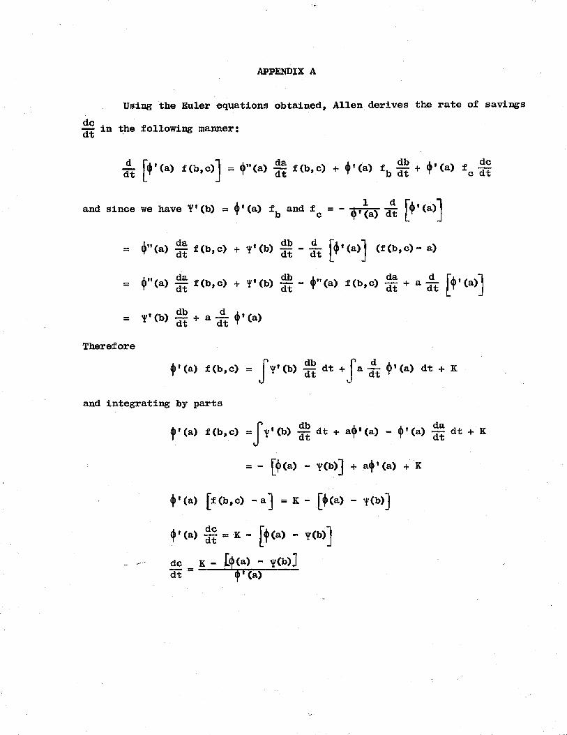
APPENDIX A
Using the Euler equations obtained, Allen derives the rate of savings
in the following maimer:dt
i [>•<») f(b,o)J = f (a) f(b,c) + V(a) £b § + f(a) £c §
and since we have (b) = <j>'(a) ffe and fc = - ^t(ay || j4'(a)J
(j>"(a) dadt f(b, c) + y’(b) db _
dt -#E [♦»(a)J (f(b,c)- a)
f ’< a) dadt f(b, c) + y*(b) db _
dt • f ’(a) „ - da f(b,c) ^ + a ddt
y’(b) dbdt + a d
dt $’(a)
Therefore
<|>'(a) f(b,c) = V ( b ) || dt + J a ± (j)'(a) dt + K
and integrating by parts
<j>'(a) f (b,c) = J V ( b ) || dt + a<|>' (a) - cf>* (a) || dt + K
= “ [<|>(a) - Y(b)j + a<j>* (a) + K
4»* <a) [f(b,c) - a] = K - j>(a) - y(b)]
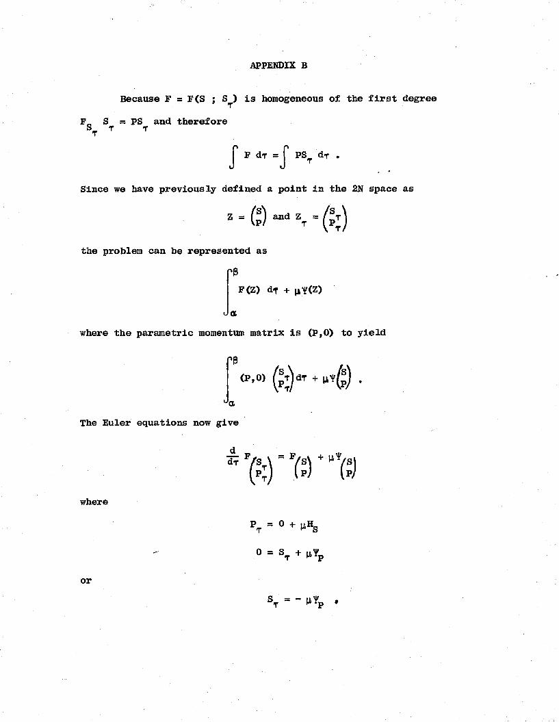
APPENDIX B
Because F = F(S ; S^) is homogeneous of the first degree
F_ S = PS and therefore S T TT
J F dT = J PST dT .
Since we have previously defined a point in the 2N space as
the problem can be represented as
’0F(Z) dt +
J<X
where the parametric momentum matrix is (P,0) to yield
The Euler equations now give
where
orsT = - »*rp

which axe the famous Hamilton first order partial differential equations
2N in number which must be solved instead of the N second order Euler
equations originally derived.


![[Concord] [Warrior Series 6514] Waffen-SS at War (1) the Early Years 1939-1942 (2006)](https://img.pdfslide.us/doc/110x75/55cf9b0b550346d033a48291/concord-warrior-series-6514-waffen-ss-at-war-1-the-early-years-1939-1942.jpg)