Embed Size (px)
Citation preview
04/18/23 EECS 584, Fall 2011 1
The Gamma Database MachineDeWitt, Ghandeharizadeh, Schneider,
Bricker, Hsiao, Rasmussen
Deepak Bastakoty
(With slide material sourced from Ghandeharizadeh and DeWitt)
04/18/23 EECS 584, Fall 2011 2
Outline
• Motivation • Physical System Designs• Data Clustering• Failure Management• Query Processing• Evaluation and Results• Bonus : Current Progress, Hadoop, Clustera..
04/18/23 EECS 584, Fall 2011 3
Outline
• Motivation • Physical System Designs• Data Clustering• Failure Management• Query Processing• Evaluation and Results• Bonus : Current Progress, Hadoop, Clustera..
04/18/23 EECS 584, Fall 2011 4
Motivation
What ?– Parallelizing Databases
• How to setup system / hardware?• How to distribute data ?• How to tailor software ?• Where does this rabbit hole lead?
04/18/23 EECS 584, Fall 2011 5
Motivation
Why ?
04/18/23 EECS 584, Fall 2011 6
Motivation
Why ?– Obtain faster response time– Increase query throughput– Improve robustness to failure– Reduce system cost– Enable Massive Scalability
(Faster, Safer, Cheaper, and More of it !)
04/18/23 EECS 584, Fall 2011 7
Outline
• Motivation • Physical System Designs• Data Clustering• Failure Management• Query Processing• Evaluation and Results• Bonus : Current Progress, Hadoop, Clustera..
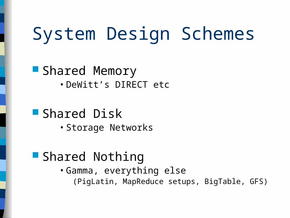
System Design Schemes
Shared Memory• DeWitt’s DIRECT etc
Shared Disk• Storage Networks
Shared Nothing• Gamma, everything else
(PigLatin, MapReduce setups, BigTable, GFS)
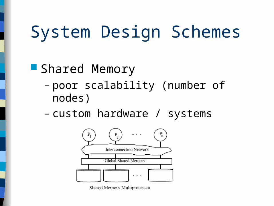
System Design Schemes
Shared Memory– poor scalability (number of nodes)– custom hardware / systems
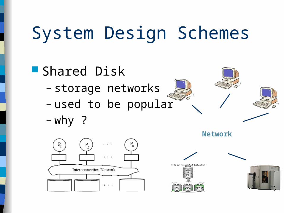
System Design Schemes
Shared Disk– storage networks– used to be popular– why ?
Network
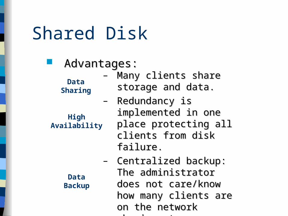
Advantages:Advantages:
HighAvailability
DataBackup
DataSharing
– Many clients share storage Many clients share storage and data.and data.
– Redundancy is Redundancy is implemented in one place implemented in one place protecting all clients from protecting all clients from disk failure.disk failure.
– Centralized backup: The Centralized backup: The administrator does not administrator does not care/know how many care/know how many clients are on the network clients are on the network sharing storage.sharing storage.
Shared Disk
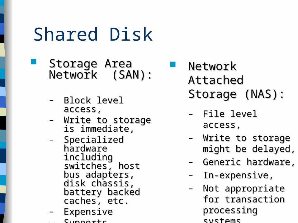
Shared Disk Storage Area Storage Area
Network (SAN):Network (SAN):
– Block level access,Block level access,– Write to storage is Write to storage is
immediate,immediate,– Specialized hardware Specialized hardware
including switches, including switches, host bus adapters, disk host bus adapters, disk chassis, battery chassis, battery backed caches, etc.backed caches, etc.
– ExpensiveExpensive– Supports transaction Supports transaction
processing systems.processing systems.
Network Attached Network Attached Storage (NAS):Storage (NAS):
– File level access,File level access,
– Write to storage might Write to storage might be delayed,be delayed,
– Generic hardware,Generic hardware,
– In-expensive,In-expensive,
– Not appropriate for Not appropriate for transaction processing transaction processing systems.systems.
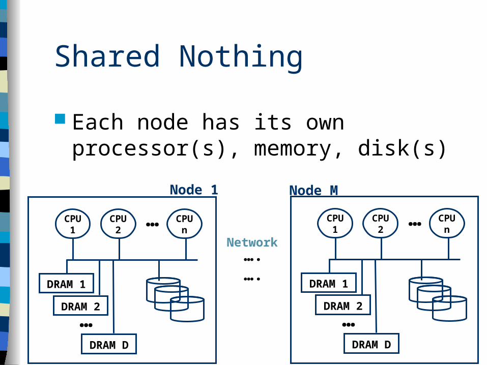
Shared Nothing
Each node has its own processor(s), memory, disk(s)
Network…. ….
CPU1
CPU2
CPUn
DRAM 1
DRAM 2
DRAM D
…
…
CPU1
CPU2
CPUn
DRAM 1
DRAM 2
DRAM D
…
…
Node MNode 1
Shared Nothing
Why ?
– Low Bandwidth Parallel Data Processing
– Commodity hardware (Cheap !!)
– Minimal Sharing = Minimal Interference
– Hence : Scalability (keep adding nodes!)
– DeWitt says : Even writing code is simpler
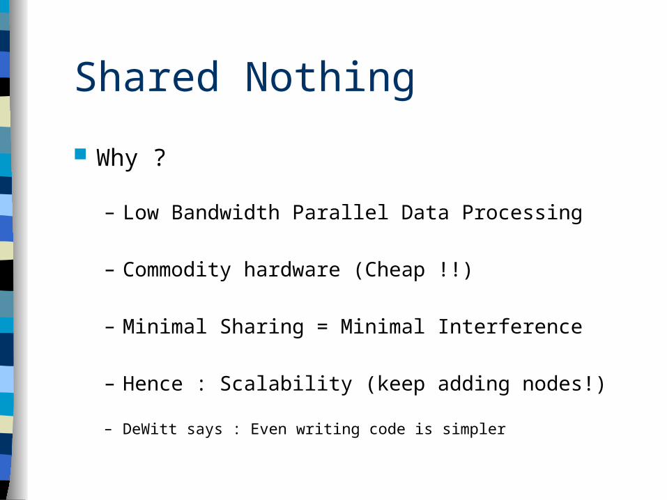
Shared Nothing
Why ?
– Low Bandwidth Parallel Data Processing
– Commodity hardware (Cheap !!)
– Minimal Sharing = Minimal Interference
– Hence : Scalability (keep adding nodes!)
– DeWitt says : Even writing code is simpler
04/18/23 EECS 584, Fall 2011 16
Outline
• Motivation • Physical System Designs• Data Clustering• Failure Management• Query Processing• Evaluation and Results• Bonus : Current Progress, Hadoop, Clustera..
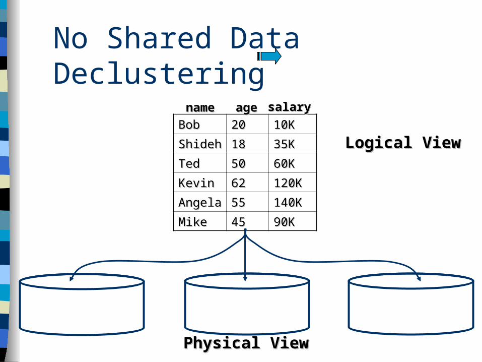
No Shared Data Declustering
Physical ViewPhysical View
BobBob 2020 10K10K
ShidehShideh 1818 35K35K
TedTed 5050 60K60K
KevinKevin 6262 120K120K
AngelaAngela 5555 140K140K
MikeMike 4545 90K90K
Logical ViewLogical View
namename ageage salarysalary
Spreading data between disks :
– Attribute-less partitioning• Random • Round-Robin
– Single Attribute Schemes• Hash De-clustering• Range De-clustering
– Multiple Attributes schemes possible• MAGIC, BERD etc
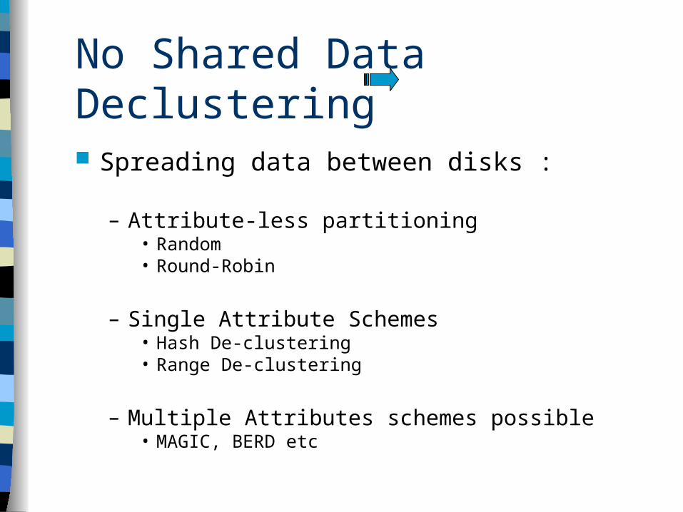
No Shared Data Declustering

Spreading data between disks :
– Attribute-less partitioning• Random • Round-Robin
– Single Attribute Schemes• Hash De-clustering• Range De-clustering
– Multiple Attributes schemes possible• MAGIC, BERD etc
No Shared Data Declustering
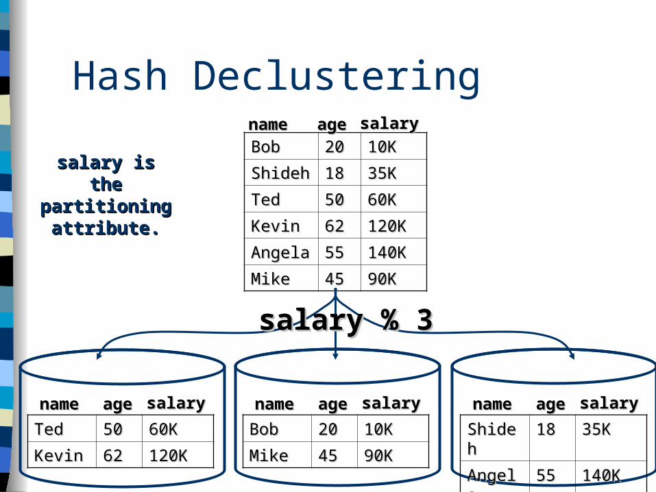
BobBob 2020 10K10K
ShidehShideh 1818 35K35K
TedTed 5050 60K60K
KevinKevin 6262 120K120K
AngelaAngela 5555 140K140K
MikeMike 4545 90K90K
namename ageage salarysalary
salary % 3salary % 3
TedTed 5050 60K60K
KevinKevin 6262 120K120K
namename ageage salarysalary
BobBob 2020 10K10K
MikeMike 4545 90K90K
namename ageage salarysalary
ShidehShideh 1818 35K35K
AngelaAngela 5555 140K140K
namename ageage salarysalary
salary is the salary is the partitioning partitioning
attribute.attribute.
Hash Declustering
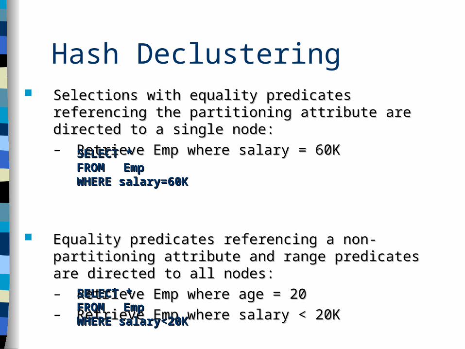
Hash Declustering Selections with equality predicates referencing the Selections with equality predicates referencing the
partitioning attribute are directed to a single node:partitioning attribute are directed to a single node:
– Retrieve Emp where salary = 60KRetrieve Emp where salary = 60K
Equality predicates referencing a non-partitioning attribute Equality predicates referencing a non-partitioning attribute and range predicates are directed to all nodes:and range predicates are directed to all nodes:
– Retrieve Emp where age = 20 Retrieve Emp where age = 20
– Retrieve Emp where salary < 20KRetrieve Emp where salary < 20K
SELECT *SELECT *FROM FROM EmpEmpWHERE salary=60KWHERE salary=60K
SELECT *SELECT *FROM FROM EmpEmpWHERE salary<20KWHERE salary<20K
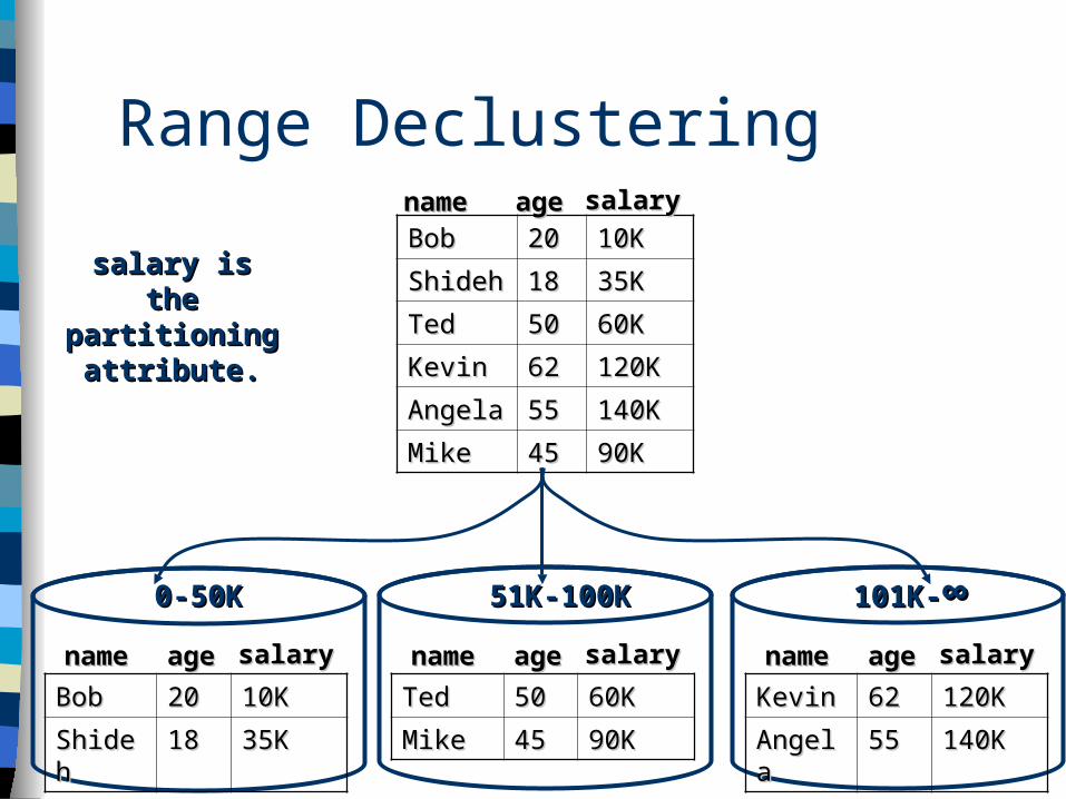
BobBob 2020 10K10K
ShidehShideh 1818 35K35K
TedTed 5050 60K60K
KevinKevin 6262 120K120K
AngelaAngela 5555 140K140K
MikeMike 4545 90K90K
namename ageage salarysalary
salary is the salary is the partitioning partitioning
attribute.attribute.
BobBob 2020 10K10K
ShidehShideh 1818 35K35K
namename ageage salarysalary
TedTed 5050 60K60K
MikeMike 4545 90K90K
namename ageage salarysalary
KevinKevin 6262 120K120K
AngelaAngela 5555 140K140K
namename ageage salarysalary
0-50K0-50K 51K-100K51K-100K 101K-101K-∞∞
Range Declustering
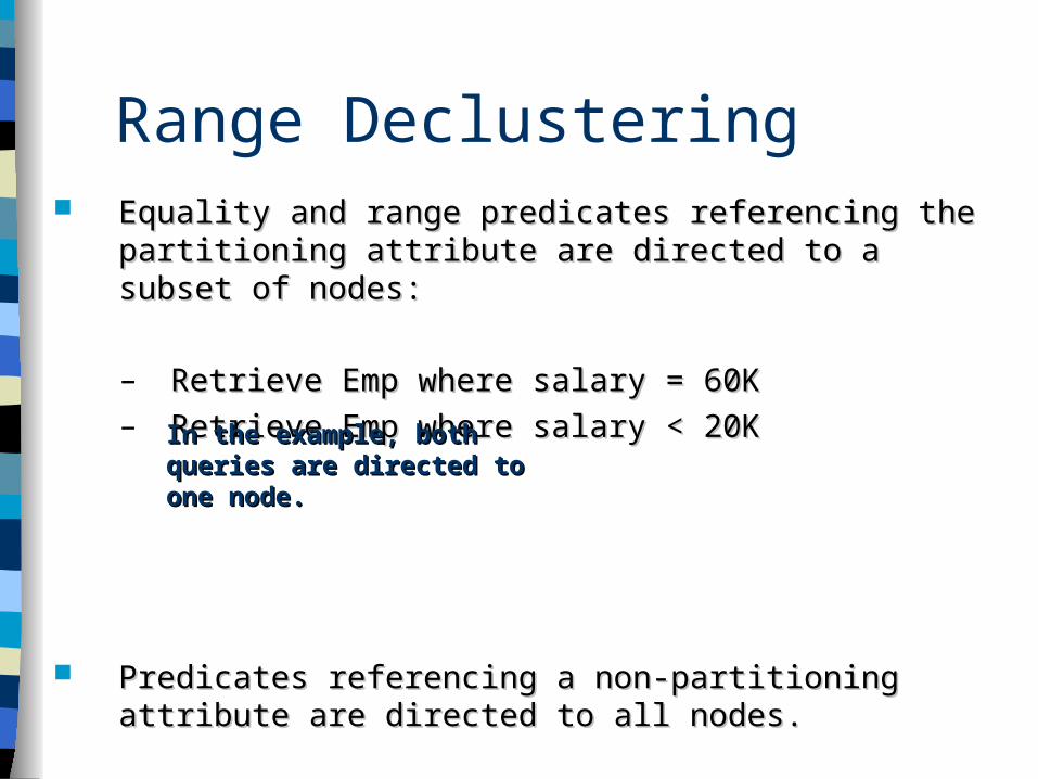
Range Declustering Equality and range predicates referencing the partitioning Equality and range predicates referencing the partitioning
attribute are directed to a subset of nodes:attribute are directed to a subset of nodes:
– Retrieve Emp where salary = 60KRetrieve Emp where salary = 60K
– Retrieve Emp where salary < 20KRetrieve Emp where salary < 20K
Predicates referencing a non-partitioning attribute are Predicates referencing a non-partitioning attribute are directed to all nodes.directed to all nodes.
In the example, both queries are In the example, both queries are directed to one node.directed to one node.
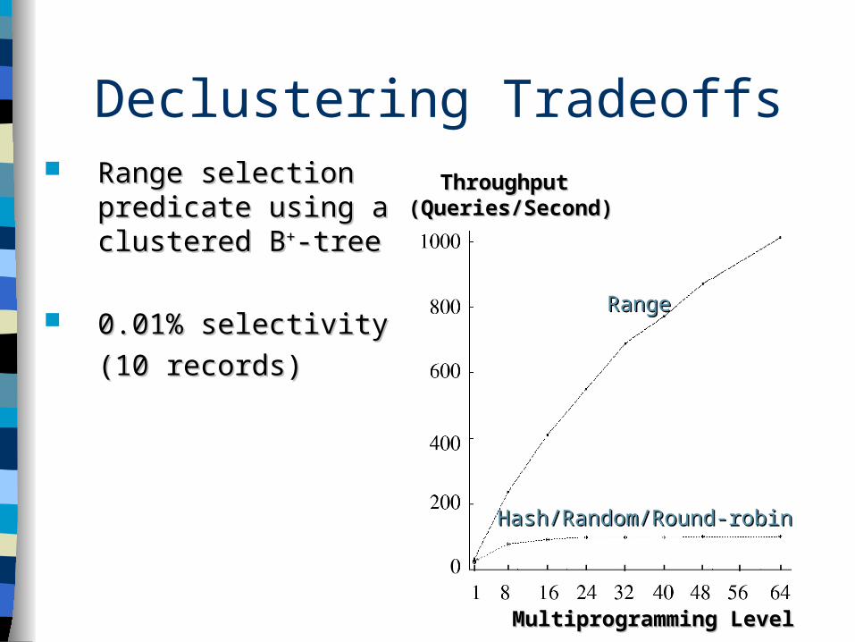
Range selection Range selection predicate using a predicate using a clustered Bclustered B++-tree-tree
0.01% selectivity 0.01% selectivity
(10 records)(10 records)
RangeRange
Hash/Random/Round-robinHash/Random/Round-robin
Multiprogramming LevelMultiprogramming Level
Throughput Throughput (Queries/Second)(Queries/Second)
Declustering Tradeoffs
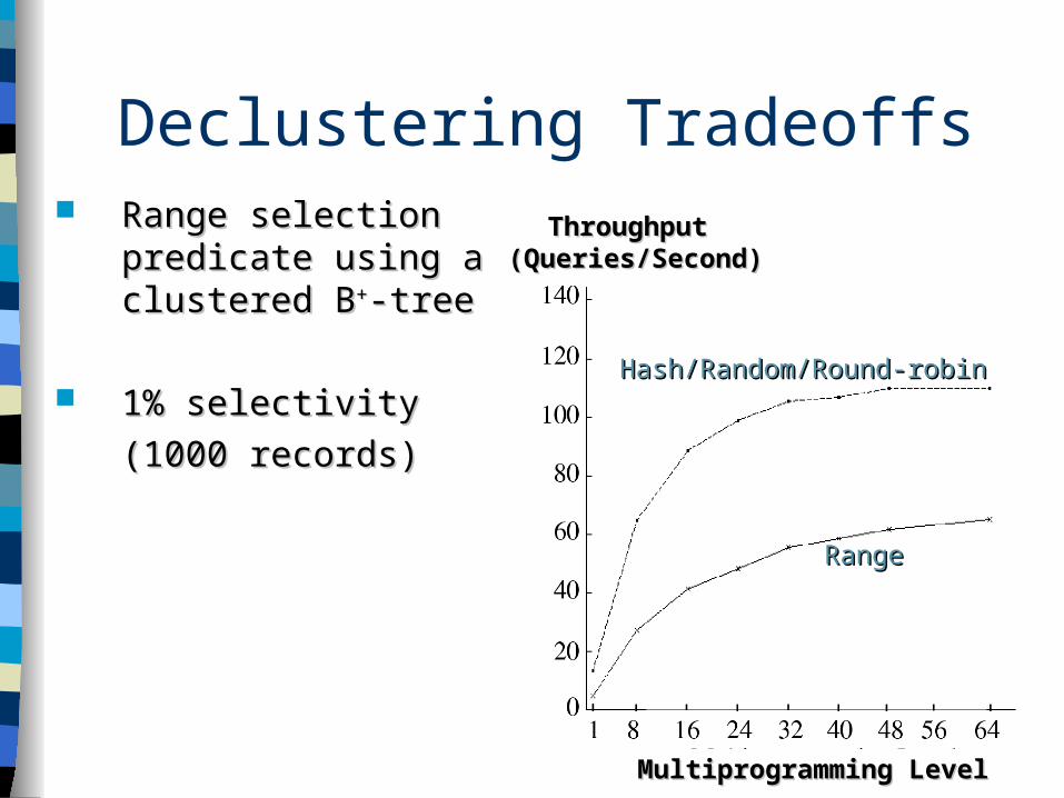
Range selection Range selection predicate using a predicate using a clustered Bclustered B++-tree-tree
1% selectivity 1% selectivity
(1000 records)(1000 records)
RangeRange
Hash/Random/Round-robinHash/Random/Round-robin
Multiprogramming LevelMultiprogramming Level
Throughput Throughput (Queries/Second)(Queries/Second)
Declustering Tradeoffs
04/18/23 EECS 584, Fall 2011 26
Why the difference ?
Declustering Tradeoffs
04/18/23 EECS 584, Fall 2011 27
Why the difference ?
• When selection was small, Range spread out load and was ideal
• When selection increased, Range caused high workload on one/few nodes while Hash spread out load
Declustering Tradeoffs
04/18/23 EECS 584, Fall 2011 28
Outline
• Motivation • Physical System Designs• Data Clustering• Failure Management• Query Processing• Evaluation and Results• Bonus : Current Progress, Hadoop, Clustera..
04/18/23 EECS 584, Fall 2011 29
Failure Management
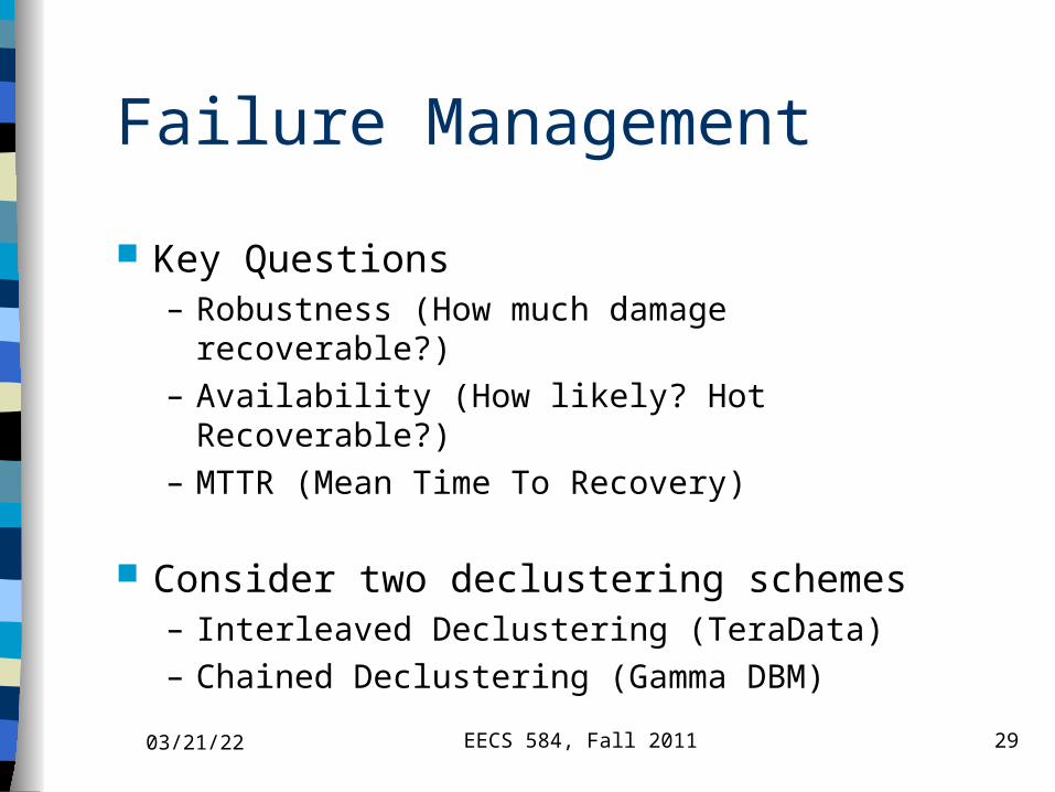
Key Questions– Robustness (How much damage recoverable?)– Availability (How likely? Hot Recoverable?)– MTTR (Mean Time To Recovery)
Consider two declustering schemes– Interleaved Declustering (TeraData)– Chained Declustering (Gamma DBM)
04/18/23 EECS 584, Fall 2011 30
Interleaved Declustering
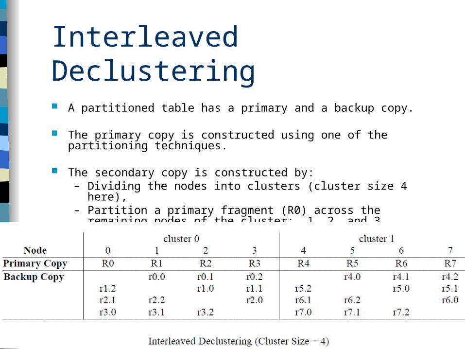
A partitioned table has a primary and a backup copy.
The primary copy is constructed using one of the partitioning techniques.
The secondary copy is constructed by:– Dividing the nodes into clusters (cluster size 4 here),– Partition a primary fragment (R0) across the remaining nodes of the
cluster: 1, 2, and 3. Realizing r0.0, r0.1, and r0.2.
Interleaved Declustering
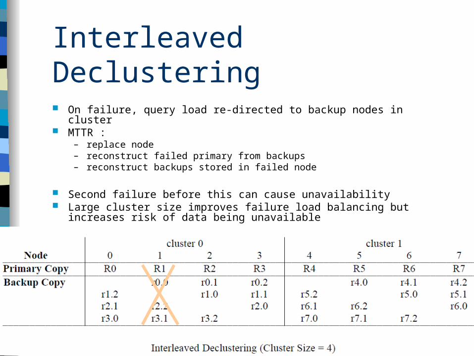
On failure, query load re-directed to backup nodes in cluster MTTR :
– replace node– reconstruct failed primary from backups– reconstruct backups stored in failed node
Second failure before this can cause unavailability Large cluster size improves failure load balancing but increases risk of
data being unavailable
Chained Declustering (Gamma)
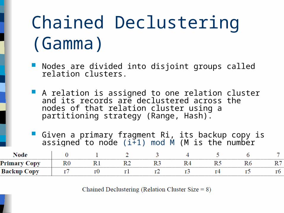
Nodes are divided into disjoint groups called relation clusters.
A relation is assigned to one relation cluster and its records are declustered across the nodes of that relation cluster using a partitioning strategy (Range, Hash).
Given a primary fragment Ri, its backup copy is assigned to node (i+1) mod M (M is the number of nodes in the relation cluster).
Chained Declustering (Gamma)
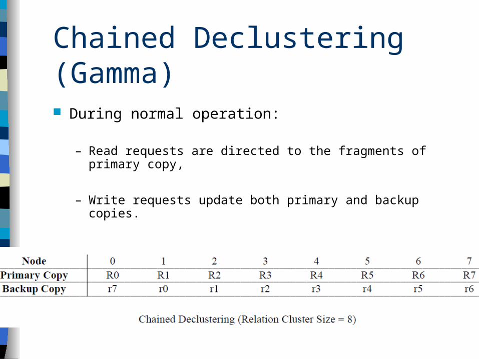
During normal operation:
– Read requests are directed to the fragments of primary copy,
– Write requests update both primary and backup copies.
Chained Declustering (Gamma)
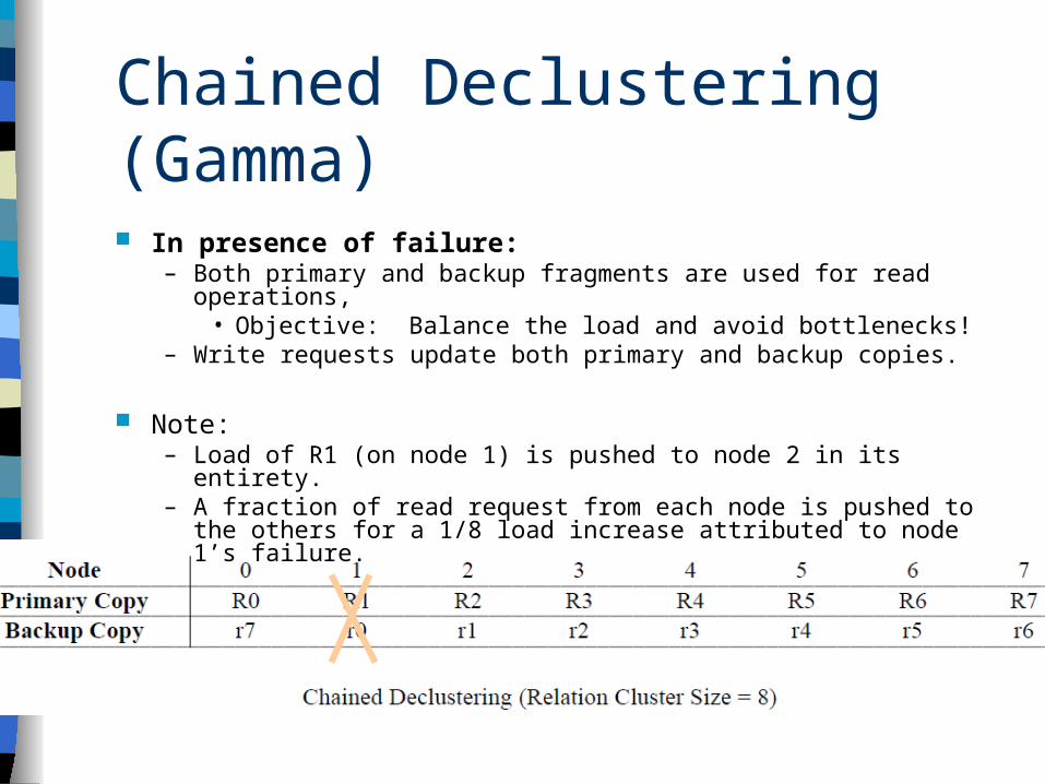
In presence of failure:– Both primary and backup fragments are used for read operations,
• Objective: Balance the load and avoid bottlenecks!– Write requests update both primary and backup copies.
Note:– Load of R1 (on node 1) is pushed to node 2 in its entirety.– A fraction of read request from each node is pushed to the others
for a 1/8 load increase attributed to node 1’s failure.
Chained Declustering (Gamma)
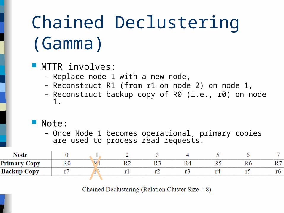
MTTR involves:– Replace node 1 with a new node,– Reconstruct R1 (from r1 on node 2) on node 1,– Reconstruct backup copy of R0 (i.e., r0) on node 1.
Note:– Once Node 1 becomes operational, primary copies are used
to process read requests.
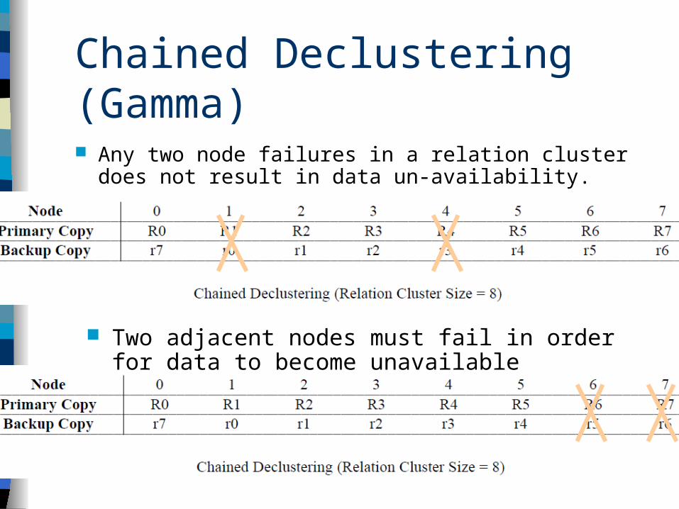
Chained Declustering (Gamma)
Any two node failures in a relation cluster does not result in data un-availability.
Two adjacent nodes must fail in order for data to become unavailable
04/18/23 EECS 584, Fall 2011 37
Outline
• Motivation • Physical System Designs• Data Clustering• Failure Management• Query Processing• Evaluation and Results• Bonus : Current Progress, Hadoop, Clustera..
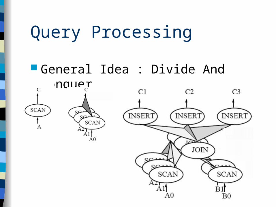
Query Processing
General Idea : Divide And Conquer
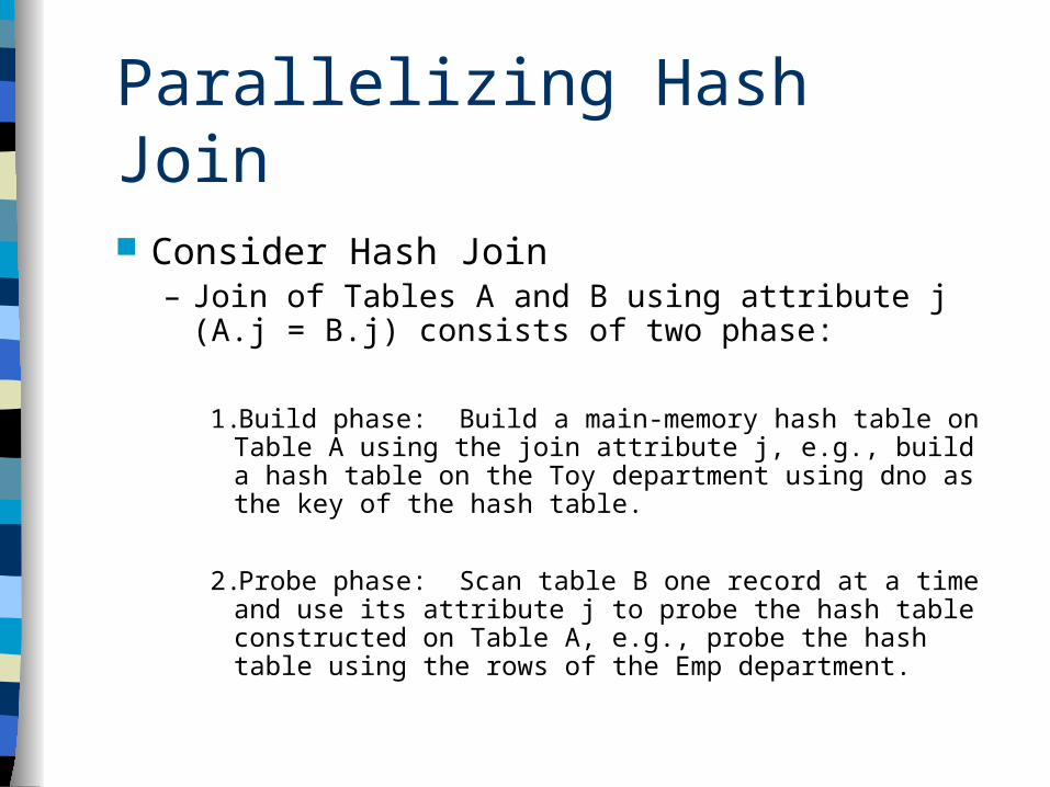
Parallelizing Hash Join
Consider Hash Join– Join of Tables A and B using attribute j (A.j = B.j)
consists of two phase:
1.Build phase: Build a main-memory hash table on Table A using the join attribute j, e.g., build a hash table on the Toy department using dno as the key of the hash table.
2.Probe phase: Scan table B one record at a time and use its attribute j to probe the hash table constructed on Table A, e.g., probe the hash table using the rows of the Emp department.

R join S where R is the inner table.
Parallelism and Hash-Join
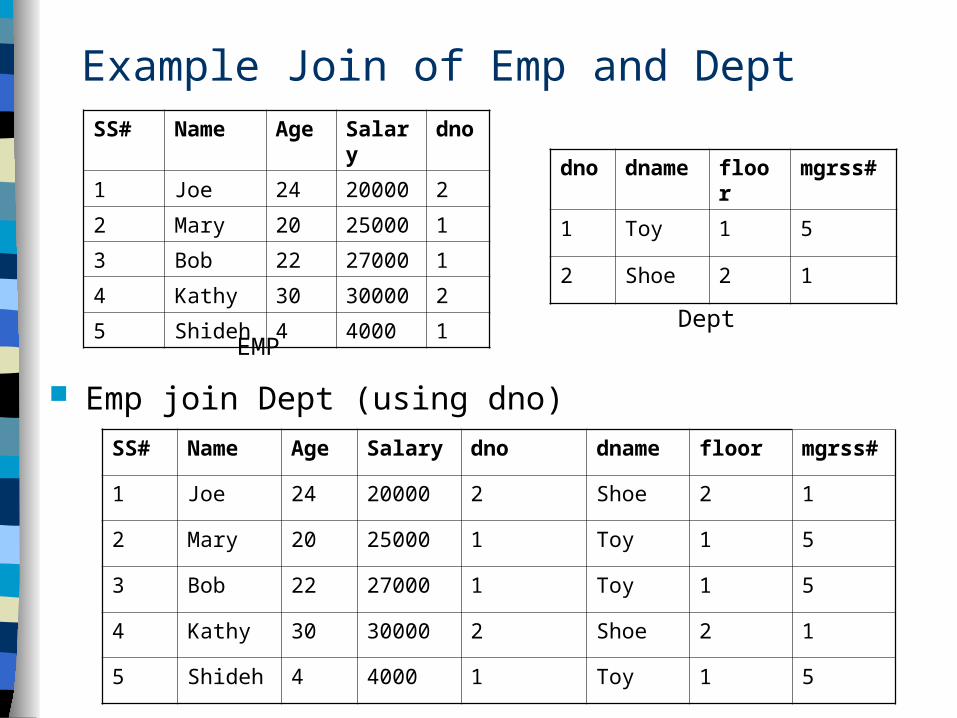
Example Join of Emp and Dept
Emp join Dept (using dno)
SS# Name Age Salary dno
1 Joe 24 20000 2
2 Mary 20 25000 1
3 Bob 22 27000 1
4 Kathy 30 30000 2
5 Shideh 4 4000 1
EMP
dno dname floor mgrss#
1 Toy 1 5
2 Shoe 2 1
Dept
SS# Name Age Salary dno dname floor mgrss#
1 Joe 24 20000 2 Shoe 2 1
2 Mary 20 25000 1 Toy 1 5
3 Bob 22 27000 1 Toy 1 5
4 Kathy 30 30000 2 Shoe 2 1
5 Shideh 4 4000 1 Toy 1 5
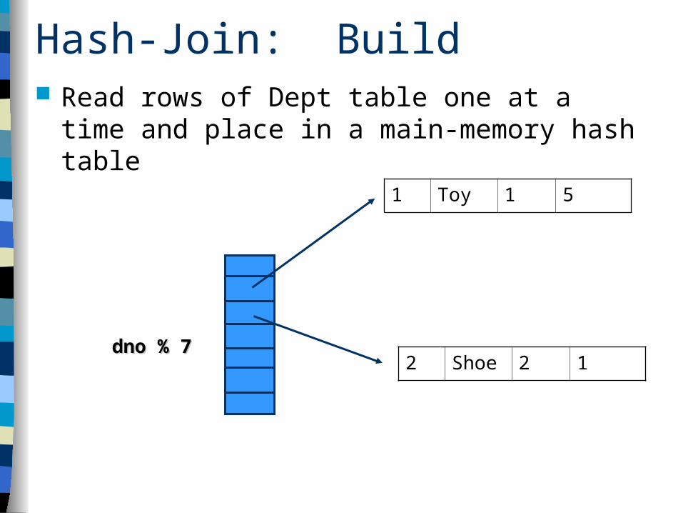
Hash-Join: Build Read rows of Dept table one at a time and place
in a main-memory hash table
1 Toy 1 5
2 Shoe 2 1dno % 7dno % 7
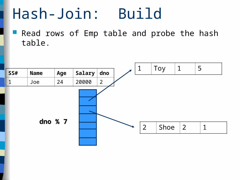
Hash-Join: Build Read rows of Emp table and probe the hash table.
1 Toy 1 5
2 Shoe 2 1dno % 7dno % 7
SS# Name Age Salary dno
1 Joe 24 20000 2
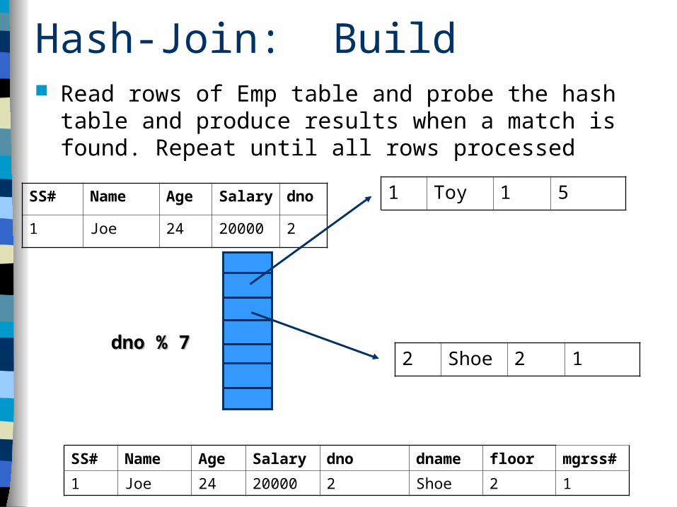
Hash-Join: Build Read rows of Emp table and probe the hash table and
produce results when a match is found. Repeat until all rows processed
SS# Name Age Salary dno
1 Joe 24 20000 2
1 Toy 1 5
2 Shoe 2 1dno % 7dno % 7
SS# Name Age Salary dno dname floor mgrss#
1 Joe 24 20000 2 Shoe 2 1
Hash-Join (slide for exam etc review only)
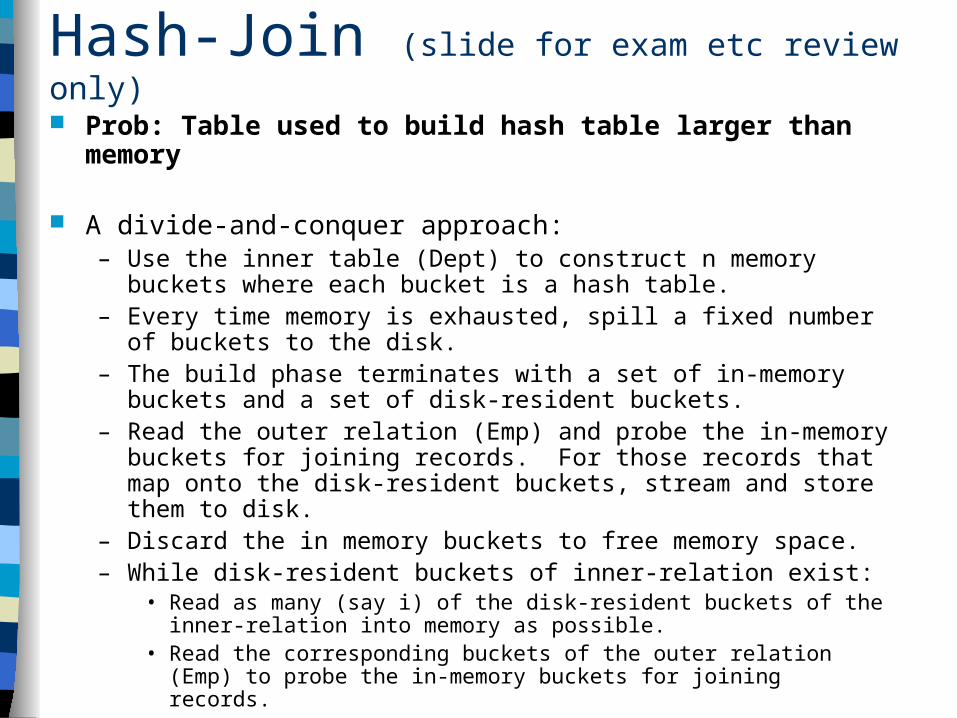
Prob: Table used to build hash table larger than memory
A divide-and-conquer approach:– Use the inner table (Dept) to construct n memory buckets where each
bucket is a hash table.– Every time memory is exhausted, spill a fixed number of buckets to the
disk.– The build phase terminates with a set of in-memory buckets and a set of
disk-resident buckets.– Read the outer relation (Emp) and probe the in-memory buckets for
joining records. For those records that map onto the disk-resident buckets, stream and store them to disk.
– Discard the in memory buckets to free memory space.– While disk-resident buckets of inner-relation exist:
• Read as many (say i) of the disk-resident buckets of the inner-relation into memory as possible.
• Read the corresponding buckets of the outer relation (Emp) to probe the in-memory buckets for joining records.
• Discard the in memory buckets to free memory space.• Delete the i buckets of the inner and outer relations.
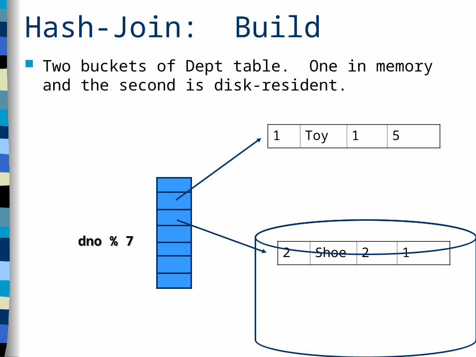
Hash-Join: Build Two buckets of Dept table. One in memory and the
second is disk-resident.
1 Toy 1 5
2 Shoe 2 1dno % 7dno % 7
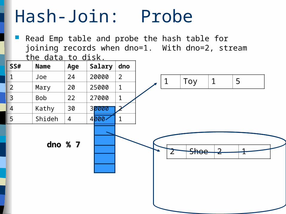
Hash-Join: Probe Read Emp table and probe the hash table for joining records when
dno=1. With dno=2, stream the data to disk.
1 Toy 1 5
2 Shoe 2 1dno % 7dno % 7
SS# Name Age Salary dno
1 Joe 24 20000 2
2 Mary 20 25000 1
3 Bob 22 27000 1
4 Kathy 30 30000 2
5 Shideh 4 4000 1
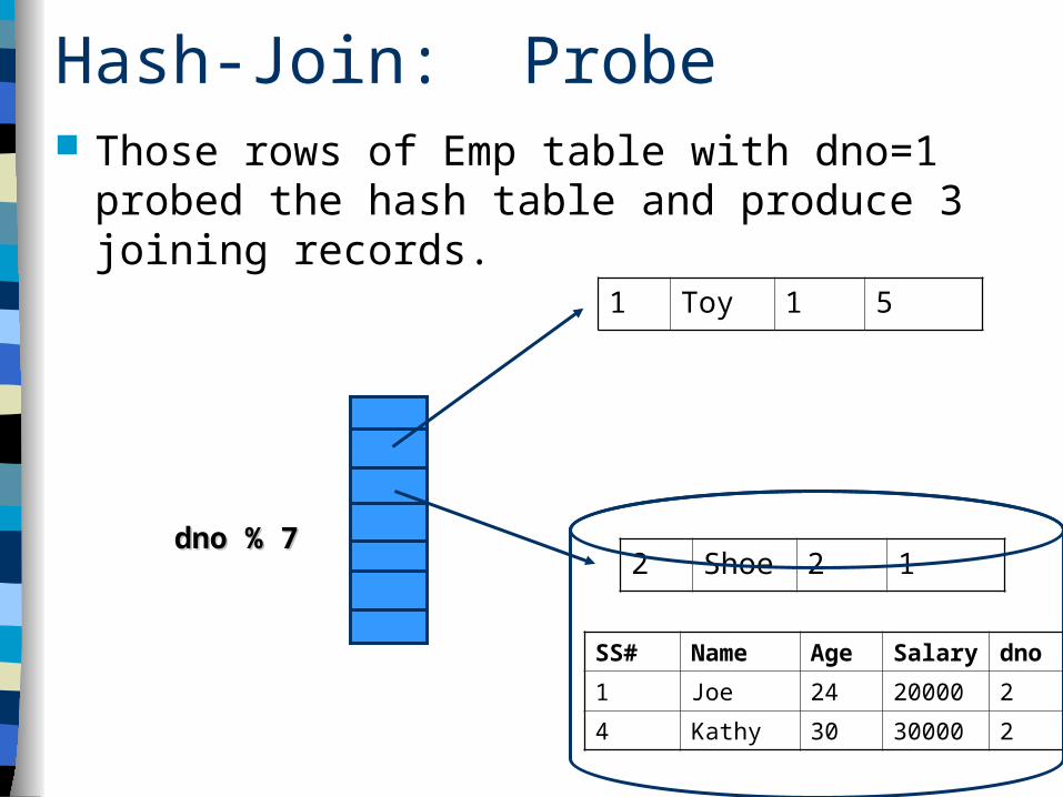
Hash-Join: Probe Those rows of Emp table with dno=1 probed the
hash table and produce 3 joining records.
1 Toy 1 5
2 Shoe 2 1dno % 7dno % 7
SS# Name Age Salary dno
1 Joe 24 20000 2
4 Kathy 30 30000 2
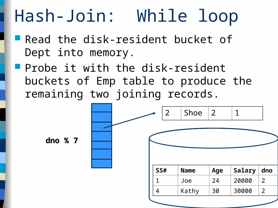
Hash-Join: While loop Read the disk-resident bucket of Dept into
memory. Probe it with the disk-resident buckets of Emp
table to produce the remaining two joining records.
2 Shoe 2 1
dno % 7dno % 7
SS# Name Age Salary dno
1 Joe 24 20000 2
4 Kathy 30 30000 2
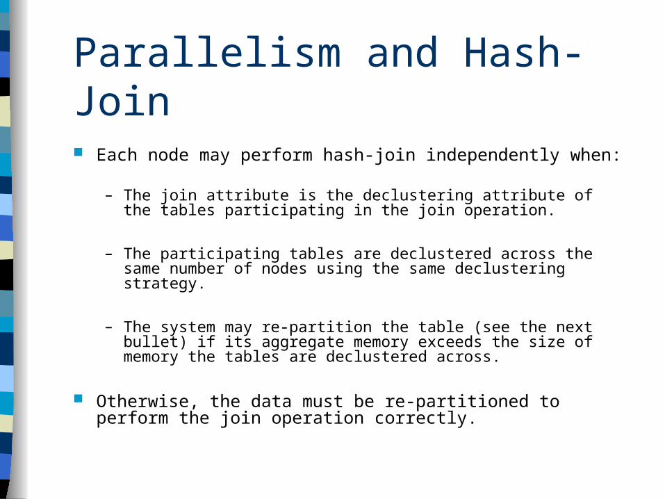
Parallelism and Hash-Join
Each node may perform hash-join independently when:
– The join attribute is the declustering attribute of the tables participating in the join operation.
– The participating tables are declustered across the same number of nodes using the same declustering strategy.
– The system may re-partition the table (see the next bullet) if its aggregate memory exceeds the size of memory the tables are declustered across.
Otherwise, the data must be re-partitioned to perform the join operation correctly.
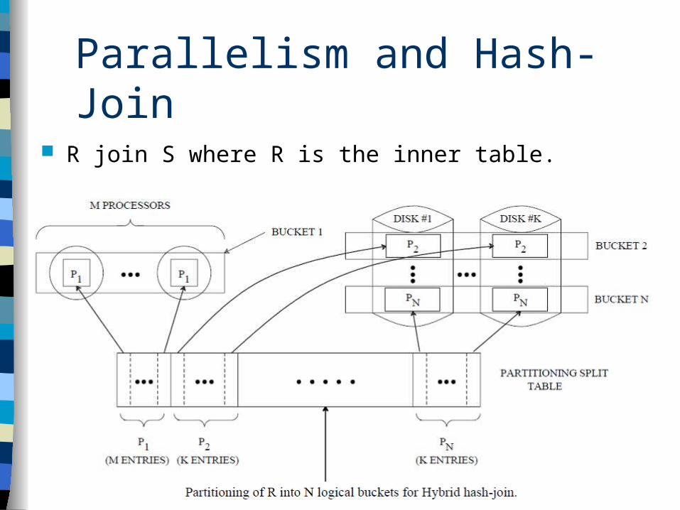
R join S where R is the inner table.
Parallelism and Hash-Join
04/18/23 EECS 584, Fall 2011 52
Outline
• Motivation • Physical System Designs• Data Clustering• Failure Management• Query Processing• Evaluation and Results• Bonus : Current Progress, Hadoop, Clustera..
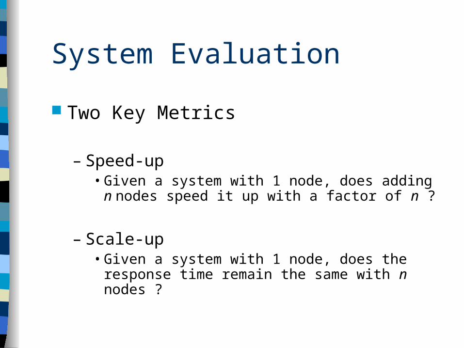
System Evaluation
Two Key Metrics
– Speed-up• Given a system with 1 node, does adding n
nodes speed it up with a factor of n ?
– Scale-up• Given a system with 1 node, does the response
time remain the same with n nodes ?
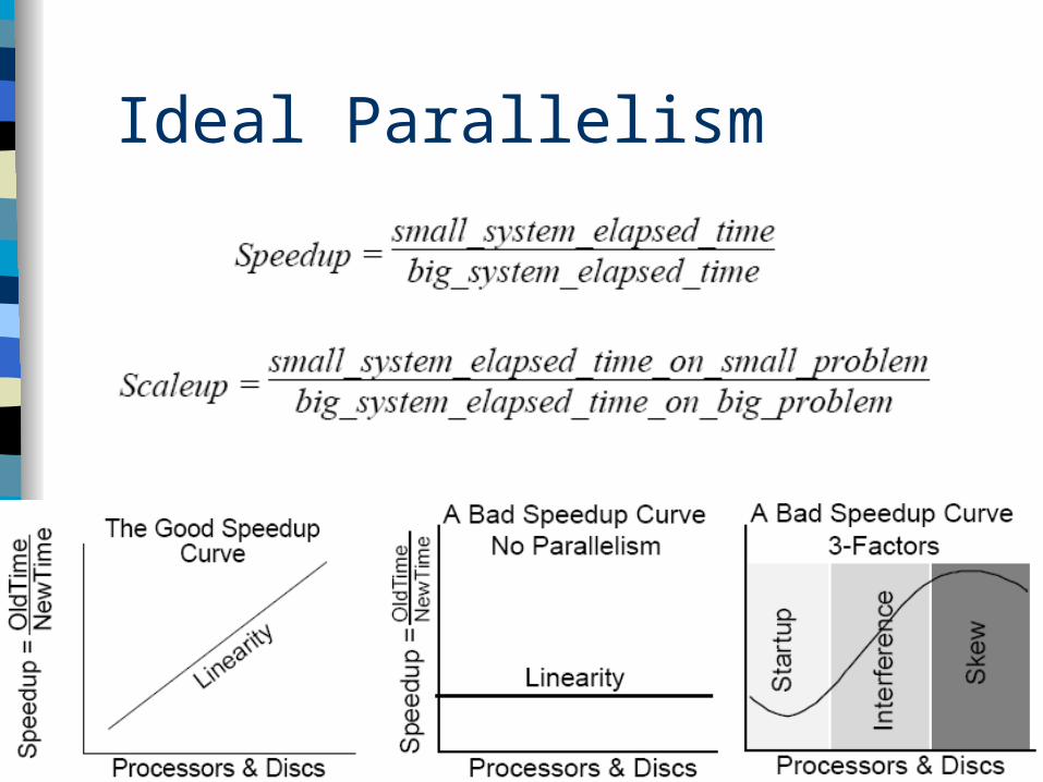
Ideal Parallelism
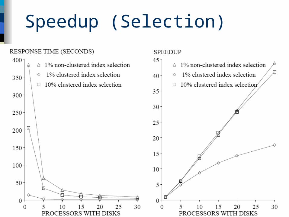
Speedup (Selection)
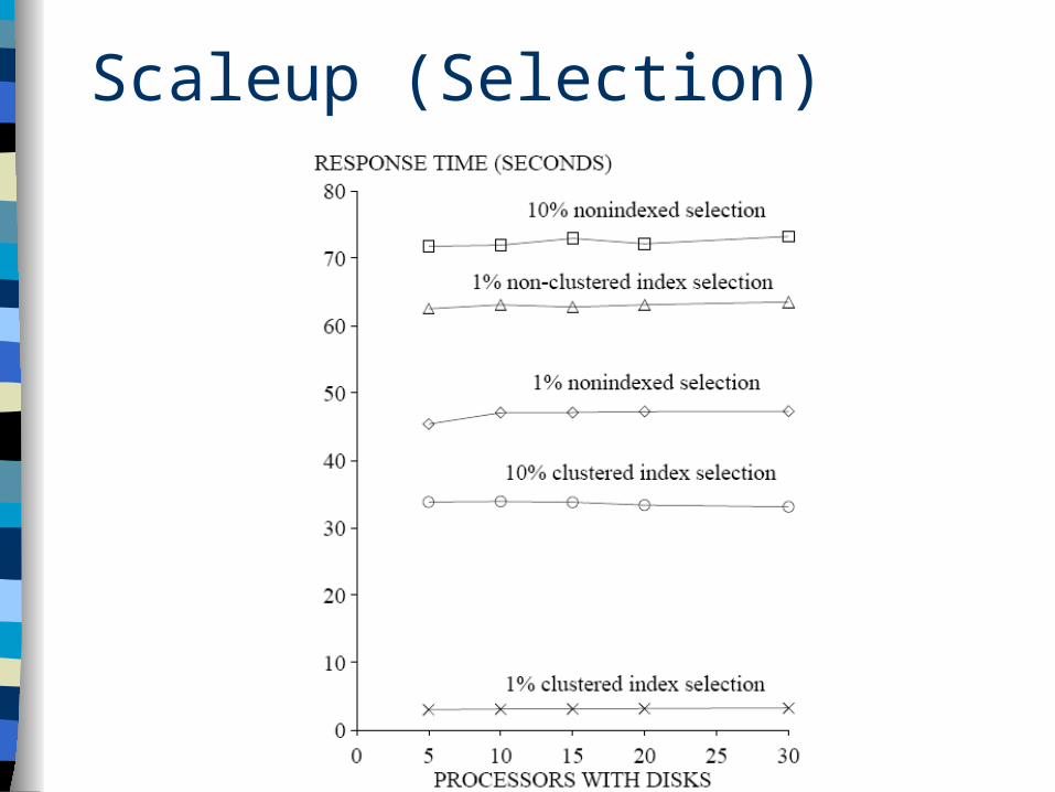
Scaleup (Selection)
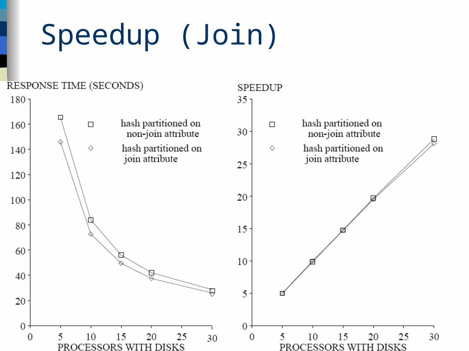
Speedup (Join)
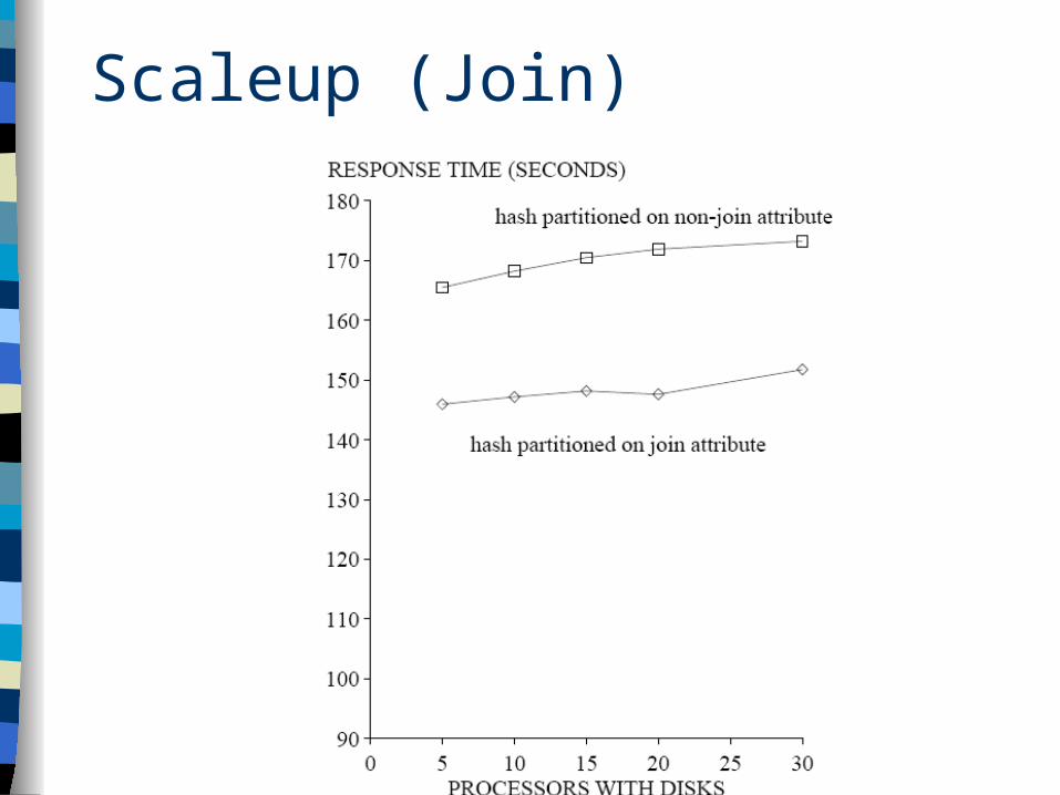
Scaleup (Join)
04/18/23 EECS 584, Fall 2011 59
Outline
• Motivation • Physical System Designs• Data Clustering• Failure Management• Query Processing• Overview of Results• Bonus: Current Progress, Hadoop, Clustera..
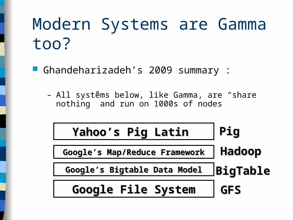
Modern Systems are Gamma too?
Ghandeharizadeh’s 2009 summary :
– All systems below, like Gamma, are “share nothing” and run on 1000s of nodes
Google File SystemGoogle File System
Google’s Bigtable Data ModelGoogle’s Bigtable Data Model
Google’s Map/Reduce FrameworkGoogle’s Map/Reduce Framework
Yahoo’s Pig Latin Yahoo’s Pig Latin
HadoopHadoop
PigPig
GFSGFS
BigTableBigTable
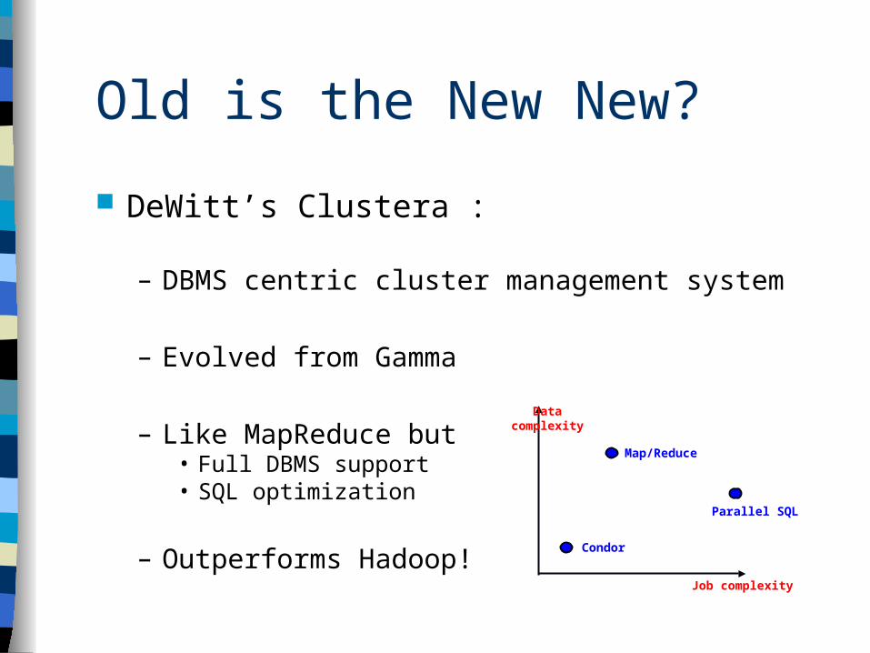
DeWitt’s Clustera :
– DBMS centric cluster management system
– Evolved from Gamma
– Like MapReduce but• Full DBMS support• SQL optimization
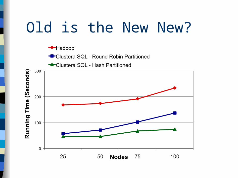
– Outperforms Hadoop!
Old is the New New?
Data complexity
Job complexity
Condor
Parallel SQL
Map/Reduce
Old is the New New?
04/18/23 EECS 584, Fall 2011 63
Outline
• Motivation • Physical System Designs• Data Clustering• Failure Management• Query Processing• Overview of Results• Bonus: Current Progress, Hadoop, Clustera..
Questions ?