6.02 Fall 2013 Lecture #3 - Massachusetts Institute of

6.02 Fall 2013 Lecture 3, Slide #1

6.02 Fall 2013�Lecture #3�

•  Communica*on network architecture •  Analog channels •  The digital abstrac*on •  Binary symmetric channels •  Hamming distance •  Channel codes


First, some recreational math related to Lecs 1 and 2�

•  Fundamental inequality: ln(x) ≤ x – 1 for x > 0 with equality only when x = 1. Proof: (Sketch LHS and RHS, to begin!) Equality for x=1 is obvious. Also, d/dx of RHS is 1, while d/dx of LHS is 1/x, which is >1 for 0 < x < 1, and is < 1 for x>1. •  So

log2(x) ≤ (x – 1).log2e for x > 0


Preceding inequality enables proofs of several results cited in Lecs 1 and 2�

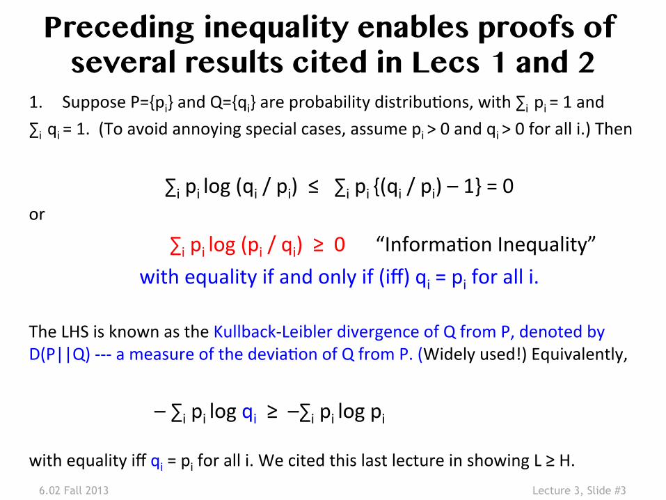
1. Suppose P={pi} and Q={qi} are probability distribu*ons, with ∑i pi = 1 and ∑i qi = 1. (To avoid annoying special cases, assume pi > 0 and qi > 0 for all i.) Then

∑i pi log (qi / pi) ≤ ∑i pi {(qi / pi) – 1} = 0 or

∑i pi log (pi / qi) ≥ 0 “Informa*on Inequality” with equality if and only if (iff) qi = pi for all i. The LHS is known as the Kullback-‐Leibler divergence of Q from P, denoted by D(P||Q) -‐-‐-‐ a measure of the devia*on of Q from P. (Widely used!) Equivalently,

– ∑i pi log qi ≥ –∑i pi log pi with equality iff qi = pi for all i. We cited this last lecture in showing L ≥ H.


More proofs …�2.  If pi > 0 for precisely i = 1 to N, then pick qi = 1/N in the

informa*on inequality to examine the divergence of the uniform distribu*on Q from P:

∑i=1 to N pi log (piNi) ≥ 0 or equivalently H = – ∑i pi log pi ≤ log N with equality iff pi = 1/N for all i. So, as previously claimed, the uniform distribu*on has maximum entropy, = log N Etc.


The System, End-to-End�

Digitize (if needed)

Original source

Source coding

Source binary digits (“message bits”)

Bit stream

COMMUNICATION NETWORK

Render/display, etc.

Receiving app/user

Source decoding

Bit stream

•  The rest of 6.02 is about the colored oval •  Simplest network is a single physical communica*on link •  We’ll start with that, then get to networks with many links


Single Link Communication Model�


Original source

Source coding


Bit stream


Receiving app/user

Source decoding

Bit stream

Channel Coding

(bit error correction)

Recv samples

+ Demapper

Mapper +

Xmit samples

Bits Signals (Voltages)

over physical link

Channel Decoding

(reducing or removing bit errors)

End-host devices

Bits


Network Communication Model�Three Abstraction Layers: Packets, Bits, Signals�


Original source

Source coding


Packets


Receiving app/user

Source decoding

Bit stream

End-host computers

Packetize

Switch Switch Switch

Switch

Buffer + stream

LINK LINK LINK

LINK

Packets Bits Signals Bits Packets

Bit stream


Physical Communication Links are Inherently Analog�

Analog = con*nuous-‐valued, con*nuous-‐*me

Voltage waveform on a cable Light on a fiber, or in free space Radio (EM) waves through the atmosphere Acous*c waves in air or water Indenta*ons on vinyl or plas*c Magne*za*on of a disc or tape …


or … Mud Pulse Telemetry, anyone?!� “This is the most common method of data transmission used by MWD (Measurement While Drilling) tools. Downhole a valve is operated to restrict the flow of the drilling mud (slurry) according to the digital informa*on to be transmiled. This creates pressure fluctua*ons represen*ng the informa*on. The pressure fluctua*ons propagate within the drilling fluid towards the surface where they are received from pressure sensors. On the surface, the received pressure signals are processed by computers to reconstruct the informa*on. The technology is available in three varie*es -‐ posi%ve pulse, nega%ve pulse, and con%nuous wave.” (from Wikipedia)


Digital Signaling: Map Bits to Signals�Key Idea: “Code” or map or modulate the desired bit sequence onto a (con*nuous-‐*me) analog signal, communica*ng at some bit rate (in bits/sec). To help us extract the intended bit sequence from the noisy received signals, we’ll map bits to signals using a fixed set of discrete values. For example, in a bi-‐level signaling (or bi-‐level mapping) scheme we use two “voltages”:

V0 is the binary value “0” V1 is the binary value “1”

If V0 = -‐V1 (and onen even otherwise) we refer to this as bipolar signaling. At the receiver, process and sample to get a “voltage” •  Voltages near V0 would be interpreted as represen*ng “0” •  Voltages near V1 would be interpreted as represen*ng “1” •  If we space V0 and V1 far enough apart, we can tolerate some degree of noise -‐-‐-‐ but there will be occasional errors!


Bit-In, Bit-Out Model of Overall Path:� Binary Symmetric Channel�

Suppose that during transmission a “0” is turned into a “1” or a “1” is turned into a “0” with probability p, independently of transmissions at other *mes This is a binary symmetric channel (BSC) -‐-‐-‐ a useful and widely used abstrac*on

0

1 with prob p

“heads” “tails”


BSC models input of “Mapper” to output of “Demapper” �


Original source

Source coding


Bit stream


Receiving app/user

Source decoding

Bit stream

Channel Coding


Recv samples

+ Demapper

Mapper +

Xmit samples

BITS Signals (Voltages)

over physical link

Channel Decoding


BITS


Replication Code to reduce decoding error �

Replication factor, n (=1/code_rate)

Prob(decoding error) over BSC w/ p=0.01

Code: Bit b coded as bb…b (n *mes) Exponen*al fall-‐off (note log scale) But huge overhead (low code rate)

We can do a lot better!


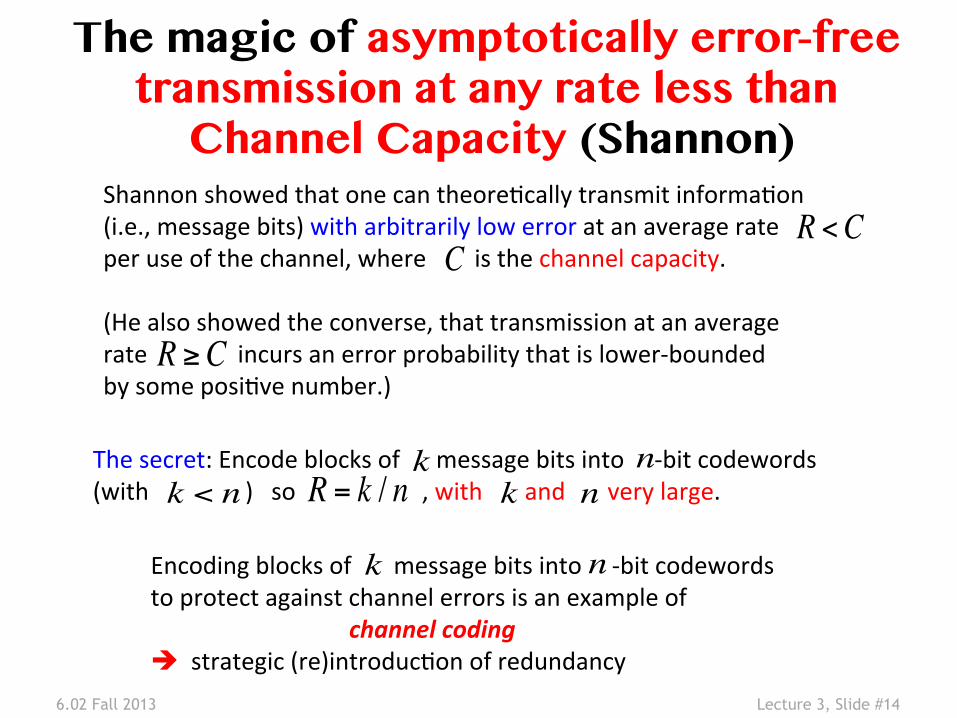
The magic of asymptotically error-free transmission at any rate less than �

Channel Capacity (Shannon)�Shannon showed that one can theore*cally transmit informa*on (i.e., message bits) with arbitrarily low error at an average rate per use of the channel, where is the channel capacity. (He also showed the converse, that transmission at an average rate incurs an error probability that is lower-‐bounded by some posi*ve number.)

R <C

R ≥C

The secret: Encode blocks of message bits into -‐bit codewords (with ) so , with and very large.

k nR = k / n nk

Encoding blocks of message bits into -‐bit codewords to protect against channel errors is an example of channel coding è strategic (re)introduc*on of redundancy

k n

C

k < n


Channel coding and decoding�


Original source

Source coding


Bit stream


Receiving app/user

Source decoding

Bit stream

Channel Coding


Recv samples

+ Demapper

Mapper +

Xmit samples

BITS Signals (Voltages)

over physical link

Channel Decoding


BITS


C =1− h(p)

è

0.5 1.0

1.0 bit per channel use

Cha

nnel

cap

acity

p

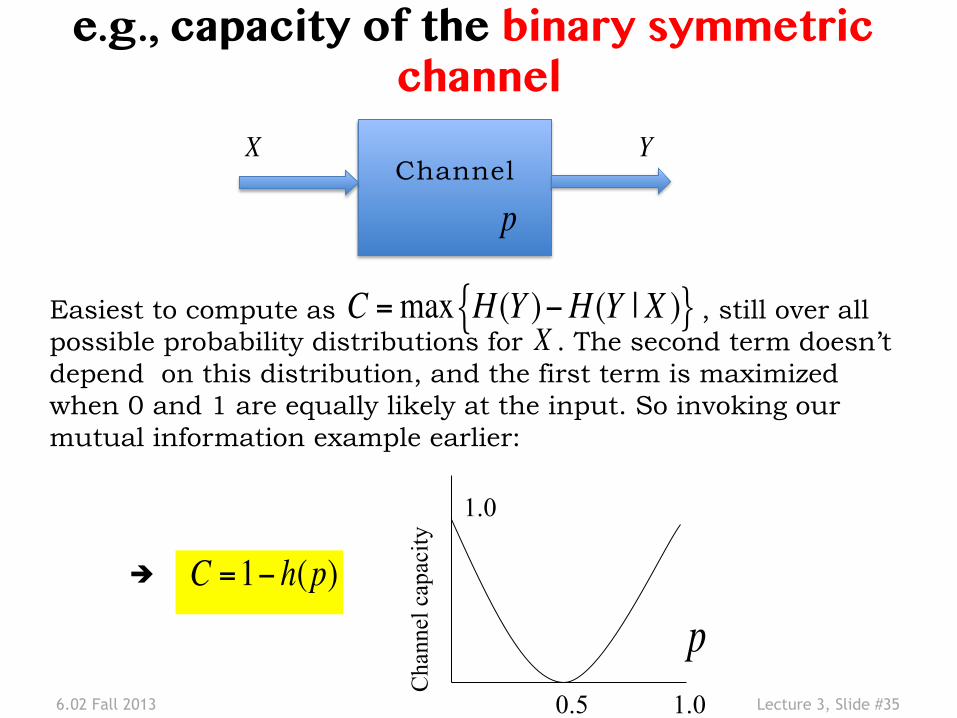
e.g., capacity of the binary symmetric channel�

C =max H (Y )−H (Y | X )}{

Channel X Y

p

X


We move on now to � �

Channel Coding�


Hamming Distance (HD)�

The number of bit posi*ons in which the corresponding bits of two binary strings of the same length are different

The Hamming Distance (HD) between a valid binary codeword and the same codeword with e errors is e. The problem with having no channel coding is that the two valid codewords (“0” and “1”) also have a Hamming distance of 1. So a single-‐bit error changes a valid codeword into another valid codeword… What is the Hamming Distance of the replica*on code?

1 0 “heads” “tails”

single-bit error

I wish he’d increase his Hamming distance


Idea: Embedding for Structural Separation�Encode so that the codewords are “far enough” from each other that the most likely error palerns don’t transform one codeword to another

11 00 “0” “1”

01

10 single-bit error may cause 00 to be 10 (or 01)

110

000 “0”

“1”

100

010

111

001

101

011

Code: nodes chosen in hypercube + mapping of message bits to nodes

If we choose 2k out of 2n nodes, it means we can map all k-‐bit message strings in a space of n-‐bit codewords. The code rate is k/n.


Minimum Hamming Distance of Code vs. �

Detection & Correction Capabilities�

If d is the minimum Hamming distance between codewords, we can detect all palerns of <= (d-‐1) bit errors

If d is the minimum Hamming distance between codewords, we can correct all palerns of

or fewer bit errors

d −12

"

#"$

%$

e.g. (schematically), a code with minimum HD=5 between two codewords (CWs) has a pair of CWs such that: [Cwi]_______X_________X_________X_________X________[CWj]


How to Construct Codes?�

Want: 4-‐bit messages with single-‐error correc*on (min HD=3) How to produce a code, i.e., a set of codewords, with this property?


A Simple Code: Parity Check �•  Add a parity bit to message of length k to make the total

number of “1” bits even (aka “even parity”). •  If the number of “1”s in the received word is odd, there there

has been an error. 0 1 1 0 0 1 0 1 0 0 1 1 → original word with parity bit 0 1 1 0 0 0 0 1 0 0 1 1 → single-‐bit error (detected) 0 1 1 0 0 0 1 1 0 0 1 1 → 2-‐bit error (not detected)

•  Minimum Hamming distance of parity check code is 2 –  Can detect all single-‐bit errors –  In fact, can detect all odd number of errors –  But cannot detect even number of errors –  And cannot correct any errors


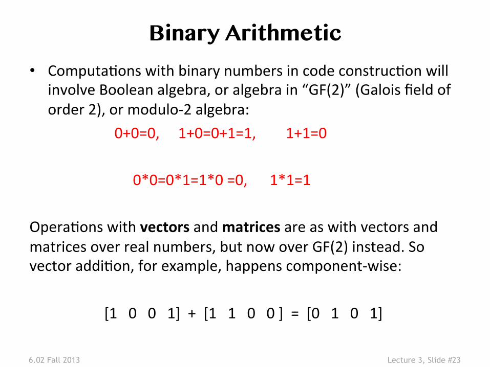
Binary Arithmetic �•  Computa*ons with binary numbers in code construc*on will

involve Boolean algebra, or algebra in “GF(2)” (Galois field of order 2), or modulo-‐2 algebra:

0+0=0, 1+0=0+1=1, 1+1=0

0*0=0*1=1*0 =0, 1*1=1 Opera*ons with vectors and matrices are as with vectors and matrices over real numbers, but now over GF(2) instead. So vector addi*on, for example, happens component-‐wise:

[1 0 0 1] + [1 1 0 0 ] = [0 1 0 1]


Linear Block Codes�

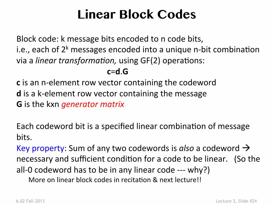
Block code: k message bits encoded to n code bits, i.e., each of 2k messages encoded into a unique n-‐bit combina*on via a linear transforma%on, using GF(2) opera*ons: c=d.G c is an n-‐element row vector containing the codeword d is a k-‐element row vector containing the message G is the kxn generator matrix Each codeword bit is a specified linear combina*on of message bits. Key property: Sum of any two codewords is also a codeword à necessary and sufficient condi*on for a code to be linear. (So the all-‐0 codeword has to be in any linear code -‐-‐-‐ why?) More on linear block codes in recita*on & next lecture!!


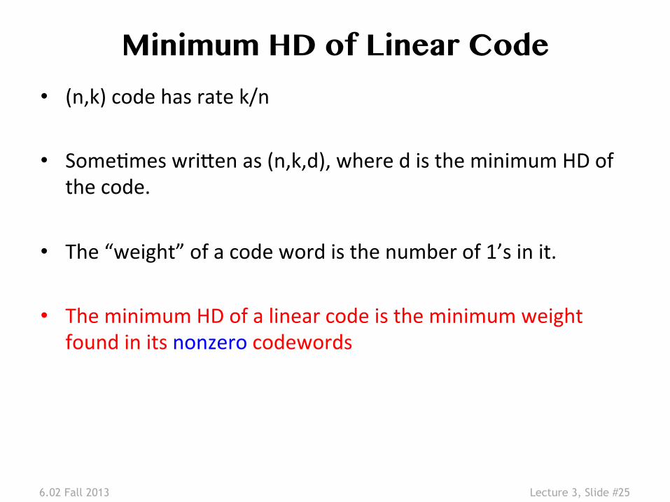
Minimum HD of Linear Code �•  (n,k) code has rate k/n

•  Some*mes wrilen as (n,k,d), where d is the minimum HD of the code.

•  The “weight” of a code word is the number of 1’s in it.

•  The minimum HD of a linear code is the minimum weight found in its nonzero codewords


Examples: What are n, k, d here?�

{000, 111} {0000, 1100, 0011, 1111}

{1111, 0000, 0001}

{1111, 0000, 0010, 1100}

Not linear codes!

The HD of a linear code is the number of “1”s in the non-‐zero codeword with the smallest # of “1”s

(3,1,3). Rate= 1/3. (4,2,2). Rate = ½.

(7,4,3) code. Rate = 4/7.


(n,k) Systematic Linear Block Codes�

•  Split data into k-‐bit blocks •  Add (n-‐k) parity bits to each block using (n-‐k) linear equa*ons,

making each block n bits long

•  Every linear code can be represented by an equivalent systema*c form

•  Corresponds to choosing G = [I | A], i.e., the iden*ty matrix in the first k columns

Message bits Parity bits

k

n The entire block is the called the “code word in systematic form”

n-k


More on channel capacity on the slides that follow��--- whatever part of this we don’t cover in lecture will be OPTIONAL reading! �


Mutual Information (Shannon)�

Channel X Y

Noise

I(X;Y ) = H (X)−H (X |Y )How much is our uncertainty about reduced by knowing ?

XY

Evidently a central ques*on in communica*on or, more generally, inference.


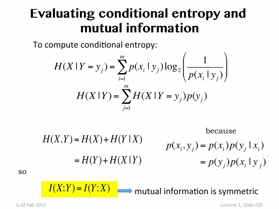
Evaluating conditional entropy and mutual information�

H (X |Y = yj ) = p(xii=1

m

∑ | yj )log21

p(xi | yj )

"

#$$

%

&''

To compute condi*onal entropy:

H (X |Y ) = H (X |Y = yj )p(j=1

m

∑ yj )

because p(xi, yj ) = p(xi )p(yj | xi )= p(yj )p(xi | y j )

I(X;Y ) = I(Y ;X)

H (X,Y ) = H (X)+H (Y | X)

= H (Y )+H (X |Y )so

mutual informa*on is symmetric


e.g., Mutual information between �input and output of �

binary symmetric channel (BSC)�

Channe l X ∈ {0,1} Y ∈ {0,1}p

With probability the input binary digit gets flipped before being presented at the output.

p

I(X;Y ) = I(Y ;X) = H (Y )−H (Y | X)=1−H (Y | X = 0)pX (0)−H (Y | X =1)pX (1)=1− h(p)

Assume 0 and 1 are equally likely


Binary entropy function �

!

Heads (or C=1) with probability Tails (or C=0) with probability

p

1− p

h(p)h(p)

p

H (C) = −p log2 p− (1− p)log2(1− p) = h(p)

1.0

0.5

1.0

0 0 0.5 1.0


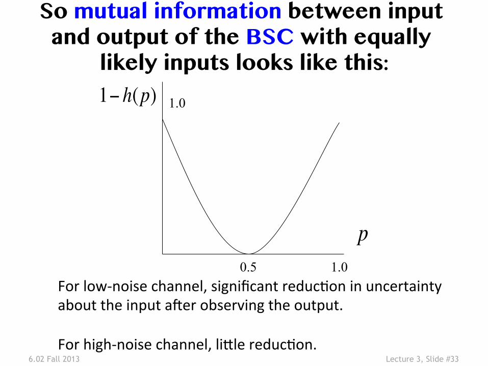
So mutual information between input and output of the BSC with equally

likely inputs looks like this:�

0.5 1.0

1.0 1− h(p)

p

For low-‐noise channel, significant reduc*on in uncertainty about the input aner observing the output. For high-‐noise channel, lille reduc*on.


Channel capacity (Shannon)�

C =max I(X;Y ) =max H (X)−H (X |Y )}{

To characterize the channel, rather than the input and output, define where the maximiza*on is over all possible distribu*ons of . XThis is the most we can expect to reduce our uncertainty about through knowledge of , and so must be the most informa%on we can expect to send through the channel on average, per use of the channel.

X Y

Channel X Y

Noise


C =1− h(p)è

0.5 1.0

1.0

Cha

nnel

cap

acity

p

e.g., capacity of the binary symmetric channel�

C =max H (Y )−H (Y | X )}{Easiest to compute as , still over all possible probability distributions for . The second term doesn’t depend on this distribution, and the first term is maximized when 0 and 1 are equally likely at the input. So invoking our mutual information example earlier:

Channel X Y

p

X

Documents

6.02 Fall 2013 Lecture #3 - Massachusetts Institute of