601.465/665 — Natural Language Processing

Assignment 6: Tagging with a Hidden Markov Model

Prof. Jason Eisner — Fall 2017Due date: Sunday 19 November, 9 pm

In this assignment, you will build a Hidden Markov Model and use it to tag words with theirparts of speech.

Collaboration: You may work in pairs on this assignment. That is, if you choose, you maycollaborate with one partner from the class, handing in a single homework with both your nameson it. However:

1. You should do all the work together, for example by pair programming. Don’t divide it upinto “my part” and “your part.”

2. Your README file should describe at the top what each of you contributed, so that we knowyou shared the work fairly.

In any case, observe academic integrity and never claim any work by third parties as your own.

Programming language: As usual, your choice, as long as we can make support for your languageavailable on the autograder. Pick a language in which you can program quickly and well, and whichprovides fast dictionaries (e.g., hash maps).

Reading: First read the handout attached to the end of this assignment!

1. The forward-backward algorithm was given in reading section C, which encouraged you toplay with the spreadsheet that we used in class.

Play as much as you like, but here are some questions to answer in your README:

(a) Reload the spreadsheet to go back to the default settings. Now, change the first day tohave just 1 ice cream.

i. What is the new probability (in the initial reconstruction) that day 1 is hot? Explain,by considering the probability of HHH versus CHH as explanations of the first threedays of data, 133.

ii. How much does this change affect the probability that day 2 is hot? That is, whatis that probability before vs. after the change to the day 1 data? What cell in thespreadsheet holds this probability?

iii. How does this change affect the final graph after 10 iterations of reestimation? Inparticular, what is p(H) on days 1 and 2? (Hint: Look at where the other 1-ice-creamdays fall during the summer.)

(b) We talked about sterotypes in class. Suppose you bring a very strong bias to interpretingthe data: you believe that I never eat only 1 ice cream on a hot day. So, again reloadthe spreadsheet, and set p(1 | H) = 0, p(2 | H) = 0.3, p(3 | H) = 0.7.

i. How does this change affect the initial reconstruction of the weather (the leftmostgraph)?

ii. What does the final graph look like after 10 iterations of reestimation?

iii. What is p(1 | H) after 10 iterations? Explain carefully why this is, discussing whathappens at each reestimation step, in terms of the 233 paths through the trellis.

(c) The backward algorithm (which computes all the β probabilities) is exactly analogous tothe inside algorithm. Recall that the inside algorithm finds the probability of a sentenceby summing over all possible parses. The backward algorithm finds the probability of asentence by summing over all possible taggings that could have generated that sentence.

i. Let’s make that precise. Each state (node) in the trellis has an β probability. Whichstate’s β probability equals the total probability of the sentence?

ii. It is actually possible to regard the backward algorithm as a special case of the insidealgorithm! In other words, there is a particular grammar whose parses correspondto taggings of the sentence. One parse of the sequence 2313 would look like the treeon the left:

START

C

H

C

H

ε

3

1

3

2

START

C

H

C

H

ε

EH

3

EC

1

EH

3

EC

2

In the tree on the left, what is the meaning of an H constituent? What is theprobability of the rule H→ 1 C? How about the probability of H→ ε? An equivalentapproach uses a grammar that instead produces the slightly more complicated parseon the right; why might one prefer that approach?

2. Write a bigram Viterbi tagger that can be run as follows on the ice cream data (readingsection F):

vtag ictrain ictest

For now, you should use naive unsmoothed estimates (i.e., maximum-likelihood estimates).The Viterbi algorithm was given in reading section D and some implementation hints weregiven in reading section H.

Your program must summarize the model’s performance on the test set, in the followingformat. These performance metrics were defined in reading section G.1.

Tagging accuracy (Viterbi decoding): 87.88% (known: 87.88% novel: 0.00%)

You are also free to print comment lines starting with #. These can report other informationthat you may want to see, including the tags your program picks, its accuracy as it goesalong, various probabilities, etc.

3. Now, you will improve your tagger so that you can run it on real data (reading section F):

vtag entrain entest

2

This means using a proper tag dictionary (for speed) and smoothed probabilities (for accu-racy).1 Ideally, your tagger should beat the following “baseline” result:

Model perplexity per tagged test word: 2649.489

Tagging accuracy (Viterbi decoding): 92.12% (known: 95.60% novel: 56.07%)

Now that you are using probabilities that are smoothed away from 0, you will have finiteperplexity. So make your program also print the perplexity, in the format shown above(see reading section G.2). This measures how surprised the model would be by the testobservations—both words and tags—before you try to reconstruct the tags from the words.

The baseline result shown above came from a stupid unigram Viterbi tagger in which thebigram transition probabilities ptt(ti | ti−1) are replaced by unigram transition probabilitiespt(ti).

2

The baseline tagger is really fast because it is a degenerate case—it throws away the tag-to-tagdependencies. If you think about what it does, it just tags every known word separately withits most probable part of speech from training data.3 Smoothing these simple probabilitieswill break ties in favor of tags that were more probable in training data; in particular, everynovel word will be tagged with the most common part of speech overall, namely N. Sincecontext is not considered, no dynamic programming is needed. It can just look up eachword token’s most probable part of speech in a hash table—with overall runtime O(n). Thisbaseline tagger also is pretty accurate (92.12%) because most words are easy to tag. To justifythe added complexity of a bigram tagger, you must show it can do better!4

Your implementation is required to use a “tag dictionary” as shown in Figure 3 of thereading—otherwise your tagger will be much too slow. Each word has a list of allowedtags, and you should consider only those tags. That is, don’t consider tag sequences that areincompatible with the dictionary.

Derive your tag dictionary from the training data. For a known word, allow only the tags thatit appeared with in the training set. For an unknown word, allow all tags except ###. (Hint:During training, before you add an observed tag t to tag dict(w) (and before incrementingc(t, w)), check whether c(t, w) > 0 already. This lets you avoid adding duplicates.)

The tag dictionary is only a form of pruning during the dynamic programming. The tagsthat are not considered will still have positive smoothed probability. Thus, even if the pruneddynamic programming algorithm doesn’t manage to consider the true (“gold”) tag sequence,that sequence will still have positive smoothed probability, which you should evaluate for theperplexity number.

1On the ic dataset, you were able to get away without smoothing because you didn’t have sparse data. You hadactually observed all possible “words” and “tags” in ictrain.

2The bigram case is the plain-vanilla definition of an HMM. It is sometimes called a 1st-order HMM, meaningthat each tag depends on 1 previous tag—just enough to make things interesting. A fancier trigram version usingpttt(ti | ti−2, ti−1) would be called a 2nd-order HMM. So by analogy, the unigram baseline can be called a 0th-orderHMM.

3That is, it chooses ti to maximize p(ti | wi). Why? Well, modifying the HMM algorithm to use unigramprobabilities says that ti−1 and ti+1 have no effect on ti. so (as you can check for yourself) the best path is justmaximizing p(ti) · p(wi | ti) at each position i separately. But that is simply the Bayes’ Theorem method formaximizing p(ti | wi).

4Comparison to a previous baseline is generally required when reporting NLP results.

3

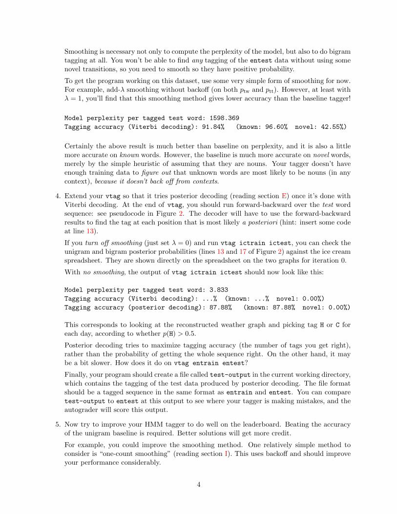
Smoothing is necessary not only to compute the perplexity of the model, but also to do bigramtagging at all. You won’t be able to find any tagging of the entest data without using somenovel transitions, so you need to smooth so they have positive probability.

To get the program working on this dataset, use some very simple form of smoothing for now.For example, add-λ smoothing without backoff (on both ptw and ptt). However, at least withλ = 1, you’ll find that this smoothing method gives lower accuracy than the baseline tagger!

Model perplexity per tagged test word: 1598.369

Tagging accuracy (Viterbi decoding): 91.84% (known: 96.60% novel: 42.55%)

Certainly the above result is much better than baseline on perplexity, and it is also a littlemore accurate on known words. However, the baseline is much more accurate on novel words,merely by the simple heuristic of assuming that they are nouns. Your tagger doesn’t haveenough training data to figure out that unknown words are most likely to be nouns (in anycontext), because it doesn’t back off from contexts.

4. Extend your vtag so that it tries posterior decoding (reading section E) once it’s done withViterbi decoding. At the end of vtag, you should run forward-backward over the test wordsequence: see pseudocode in Figure 2. The decoder will have to use the forward-backwardresults to find the tag at each position that is most likely a posteriori (hint: insert some codeat line 13).

If you turn off smoothing (just set λ = 0) and run vtag ictrain ictest, you can check theunigram and bigram posterior probabilities (lines 13 and 17 of Figure 2) against the ice creamspreadsheet. They are shown directly on the spreadsheet on the two graphs for iteration 0.

With no smoothing, the output of vtag ictrain ictest should now look like this:

Model perplexity per tagged test word: 3.833

Tagging accuracy (Viterbi decoding): ...% (known: ...% novel: 0.00%)

Tagging accuracy (posterior decoding): 87.88% (known: 87.88% novel: 0.00%)

This corresponds to looking at the reconstructed weather graph and picking tag H or C foreach day, according to whether p(H) > 0.5.

Posterior decoding tries to maximize tagging accuracy (the number of tags you get right),rather than the probability of getting the whole sequence right. On the other hand, it maybe a bit slower. How does it do on vtag entrain entest?

Finally, your program should create a file called test-output in the current working directory,which contains the tagging of the test data produced by posterior decoding. The file formatshould be a tagged sequence in the same format as entrain and entest. You can comparetest-output to entest at this output to see where your tagger is making mistakes, and theautograder will score this output.

5. Now try to improve your HMM tagger to do well on the leaderboard. Beating the accuracyof the unigram baseline is required. Better solutions will get more credit.

For example, you could improve the smoothing method. One relatively simple method toconsider is “one-count smoothing” (reading section I). This uses backoff and should improveyour performance considerably.

4

Or you could try using a higher-order HMM, e.g., trigram transition probabilities instead ofbigrams.

Or you could use a more interesting emission model that considers word spellings (e.g., wordendings) to help with novel words. Maybe the word actuary is a noun because it ends in ry,or because actuaries appears in training data as a noun. Feel free to talk to the course staffabout how to structure such a model.

We have not provided separate dev data: so if you want to tune any hyperparameters suchas smoothing parameters, you will have to split the training data into train and dev portionsfor yourself (e.g., using k-fold cross-validation). Of course, don’t use the test data to trainyour system.

Your tagger might still fall short of the state-of-the-art 97%, even though the reduced tagsetin Figure 4 of the reading ought to make the problem easier. Why? Because you only have100,000 words of training data.

How much did your tagger improve on the accuracy and perplexity of the baseline tagger (seepage 3)? Answer in your README with your observations and results, including the requiredoutput from running vtag entrain entest. Submit the source code for this version of vtag.Remember, for full credit, your tagger should include a tag dictionary, and both Viterbi andposterior decoders.

In this assignment, the leaderboard will show the various performance numbers that yourcode prints out. The autograder will probably run your code on the same entest that youhave in your possession. This is really “dev-test” data because it is being used to help developeveryone’s systems.

For actual grading, however, we will evaluate your code on “final-test” data that you havenever seen (as in Assignment 3). The autograder will run your code to both train and testyour model. It will compare the actual test-output generated by your posterior decoder tothe gold-standard tags on the final-test data.

6. Now let’s try the EM algorithm. Copy vtag to a new program, vtagem, and modify it toreestimate the HMM parameters on raw (untagged) data.5 You should be able to run it as

vtagem entrain25k entest enraw

Here entrain25k is a shorter version of entrain. In other words, let’s suppose that you don’thave much supervised data, so your tagger does badly and you need to use the unsuperviseddata in enraw to improve it.

Your EM program will alternately tag the test data (using your Viterbi decoder) and modifythe training counts. So you will be able to see how successive steps of EM help or hurt theperformance on test data.

Again, you’ll use the forward-backward algorithm, but it should now be run on the raw data.(Don’t bother running it on the test data anymore—unlike vtag, vtagem does not have toreport posterior decoding on test data.)

The forward-backward algorithm was given in reading section C and some implementationhints for EM were given in reading section J.

5Or if you prefer, you can submit a single program that behaves like vtag when given two files (train, test) andlike vtagem when given three files (train, test, raw).

5

[read train][read test][read raw][decode the test data]

Model perplexity per tagged test word: ...

Tagging accuracy (Viterbi decoding): ...% (known: ...% seen: ...% novel: ...%)

[compute new counts via forward-backward algorithm on raw]Iteration 0: Model perplexity per untagged raw word: ...

[switch to using the new counts][re-decode the test data]

Model perplexity per tagged test word: ...

Tagging accuracy (Viterbi decoding): ...% (known: ...% seen: ...% novel: ...%)

[compute new counts via forward-backward algorithm on raw]Iteration 1: Model perplexity per untagged raw word: ...

[switch to using the new counts][re-decode the test data]

Model perplexity per tagged test word: ...

Tagging accuracy (Viterbi decoding): ...% (known: ...% seen: ...% novel: ...%)

[compute new counts via forward-backward algorithm on raw]Iteration 2: Model perplexity per untagged raw word: ...

[switch to using the new counts][re-decode the test data]

Model perplexity per tagged test word: ...Tagging accuracy (Viterbi decoding): ...% (known: ...% seen: ...% novel: ...%)

[compute new counts via forward-backward algorithm on raw]Iteration 3: Model perplexity per untagged raw word: ...

[switch to using the new counts]

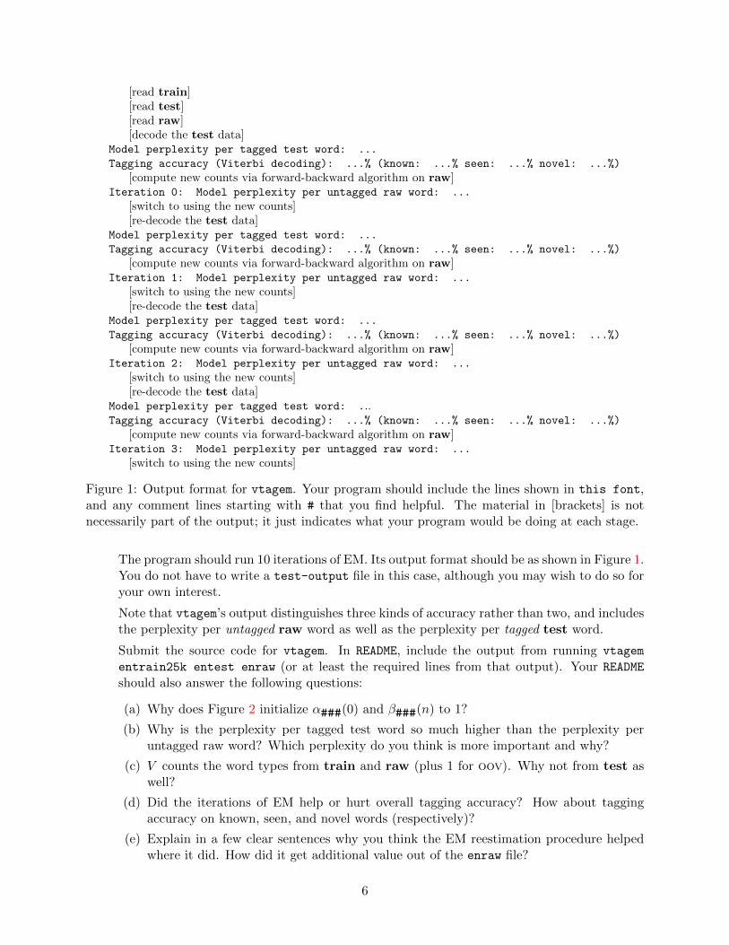
Figure 1: Output format for vtagem. Your program should include the lines shown in this font,and any comment lines starting with # that you find helpful. The material in [brackets] is notnecessarily part of the output; it just indicates what your program would be doing at each stage.

The program should run 10 iterations of EM. Its output format should be as shown in Figure 1.You do not have to write a test-output file in this case, although you may wish to do so foryour own interest.

Note that vtagem’s output distinguishes three kinds of accuracy rather than two, and includesthe perplexity per untagged raw word as well as the perplexity per tagged test word.

Submit the source code for vtagem. In README, include the output from running vtagem

entrain25k entest enraw (or at least the required lines from that output). Your README

should also answer the following questions:

(a) Why does Figure 2 initialize α###(0) and β###(n) to 1?

(b) Why is the perplexity per tagged test word so much higher than the perplexity peruntagged raw word? Which perplexity do you think is more important and why?

(c) V counts the word types from train and raw (plus 1 for oov). Why not from test aswell?

(d) Did the iterations of EM help or hurt overall tagging accuracy? How about taggingaccuracy on known, seen, and novel words (respectively)?

(e) Explain in a few clear sentences why you think the EM reestimation procedure helpedwhere it did. How did it get additional value out of the enraw file?

6

(f) Suggest at least two reasons to explain why EM didn’t always help.

(g) What is the maximum amount of ice cream you have ever eaten in one day? Why? Didyou get sick?

As mentioned in class, Merialdo (1994) found that although the EM algorithm improveslikelihood at every iteration, the tags start looking less like parts of speech after the firstfew iterations, so the tagging accuracy will get worse even though the perplexity improves.His paper at http://aclweb.org/anthology/J94-2001 has been cited 700 times, often bypeople who are attempting to build better unsupervised learners!

7. Extra credit: vtagem will be quite slow on the cz dataset. Why? Czech is a morphologicallycomplex language: each word contains several morphemes. Since its words are more compli-cated, more of them are unknown (50% instead of 9%) and we need more tags (66 insteadof 25).6 So there are (66/25)2 ≈ 7 times as many tag bigrams . . . and the worst case of twounknown words in a row (which forces us to consider all those tag bigrams) occurs far moreoften.

Speed up vtagem by implementing some kind of tag pruning during the computations of µ, α,and β. (Feel free to talk to the course staff about your ideas.) Submit your improved sourcecode. Answer the following questions in your README:

(a) Using your sped-up program, what accuracy and perplexity do you obtain for the czdataset?

(b) Estimate your speedup on the en and cz datasets.

(c) But how seriously does pruning hurt your accuracy and perplexity? Estimate this bytesting on the en dataset with and without pruning.

(d) How else could you cope with tagging a morphologically complex language like Czech?You can assume that you have a morphological analyzer for the language.

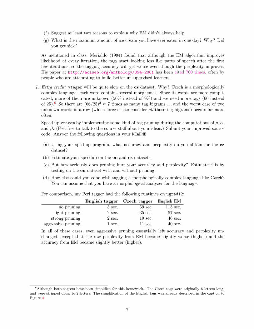
For comparison, my Perl tagger had the following runtimes on ugrad12:

English tagger Czech tagger English EM

no pruning 3 sec. 59 sec. 113 sec.light pruning 2 sec. 35 sec. 57 sec.

strong pruning 2 sec. 19 sec. 46 sec.aggressive pruning 1 sec. 11 sec. 40 sec.

In all of these cases, even aggressive pruning essentially left accuracy and perplexity un-changed, except that the raw perplexity from EM became slightly worse (higher) and theaccuracy from EM became slightly better (higher).

6Although both tagsets have been simplified for this homework. The Czech tags were originally 6 letters long,and were stripped down to 2 letters. The simplification of the English tags was already described in the caption toFigure 4.

7

601.465/665 — Natural Language Processing

Reading for Assignment 5: Tagging with a Hidden Markov Model

Prof. Jason Eisner — Fall 2017

We don’t have a required textbook for this course. Instead, handouts like this one are the mainreadings. This handout accompanies assignment 5, which refers to it.

A Semi-Supervised Learning

In the first part of the assignment, you will do supervised learning, estimating the parametersp(tag | previous tag) and p(word | tag) from a training set of already-tagged text. Some smoothingis necessary. You will then evaluate the learned model by finding the Viterbi tagging (i.e., best tagsequence) for some test data and measuring how many tags were correct.

Then in the second part of the assignment, you will try to improve your supervised parametersby reestimating them on additional “raw” (untagged) data, using the Expectation-Maximization(EM) algorithm. This yields a semi-supervised model, which you will again evaluate by findingthe Viterbi tagging on the test data. Note that you’ll use the Viterbi approximation for testing butnot for training—you’ll do real EM training using the full forward-backward algorithm.

This kind of procedure is common. Will it work in this case? For speed and simplicity, you willuse relatively small datasets, and a bigram model instead of a trigram model. You will also ignorethe spelling of words (useful for tagging unknown words). All these simplifications hurt accuracy.1

So overall, your percentage of correct tags will be in the low 90’s instead of the high 90’s that Imentioned in class.

How about speed? My final program was about 300 lines in Perl. Running on ugrad12, ithandled the final “vtag” task from question 5 in about 3 seconds, and the final “vtagem” task fromquestion 6 in under 2 minutes. Note that a compiled language should run far faster.

B Notation

In this reading handout, I’ll use the following notation. You might want to use the same notationin your program.

• The input string consists of n+ 1 words, w0, w1, . . . wn.

• The corresponding tags are t0, t1, . . . tn. We have wi/ti = ###/### for i = 0, for i = n, andprobably also for some other values of i.

• I’ll use “tt” to name tag-to-tag transition probabilities, as in ptt(ti | ti−1).

• I’ll use “tw” to name tag-to-word emission probabilities, as in ptw(wi | ti).1But another factor helps your accuracy measurement: you will also use a smaller-than-usual set of tags. The

motivation is speed, but it has the side effect that your tagger won’t have to make fine distinctions.

R-1

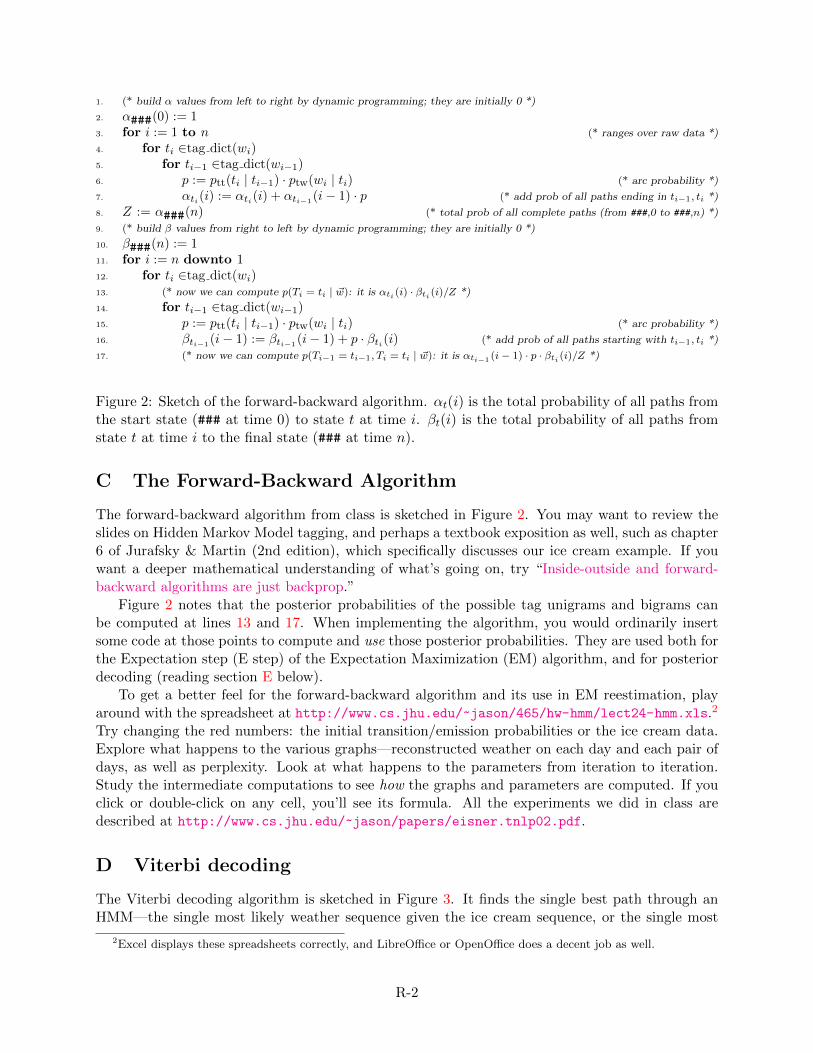
1. (* build α values from left to right by dynamic programming; they are initially 0 *)

2. α###(0) := 13. for i := 1 to n (* ranges over raw data *)

4. for ti ∈tag dict(wi)5. for ti−1 ∈tag dict(wi−1)6. p := ptt(ti | ti−1) · ptw(wi | ti) (* arc probability *)

7. αti(i) := αti(i) + αti−1(i− 1) · p (* add prob of all paths ending in ti−1, ti *)

8. Z := α###(n) (* total prob of all complete paths (from ###,0 to ###,n) *)

9. (* build β values from right to left by dynamic programming; they are initially 0 *)

10. β###(n) := 111. for i := n downto 112. for ti ∈tag dict(wi)13. (* now we can compute p(Ti = ti | ~w): it is αti (i) · βti (i)/Z *)

14. for ti−1 ∈tag dict(wi−1)15. p := ptt(ti | ti−1) · ptw(wi | ti) (* arc probability *)

16. βti−1(i− 1) := βti−1

(i− 1) + p · βti(i) (* add prob of all paths starting with ti−1, ti *)

17. (* now we can compute p(Ti−1 = ti−1, Ti = ti | ~w): it is αti−1 (i− 1) · p · βti (i)/Z *)

Figure 2: Sketch of the forward-backward algorithm. αt(i) is the total probability of all paths fromthe start state (### at time 0) to state t at time i. βt(i) is the total probability of all paths fromstate t at time i to the final state (### at time n).

C The Forward-Backward Algorithm

The forward-backward algorithm from class is sketched in Figure 2. You may want to review theslides on Hidden Markov Model tagging, and perhaps a textbook exposition as well, such as chapter6 of Jurafsky & Martin (2nd edition), which specifically discusses our ice cream example. If youwant a deeper mathematical understanding of what’s going on, try “Inside-outside and forward-backward algorithms are just backprop.”

Figure 2 notes that the posterior probabilities of the possible tag unigrams and bigrams canbe computed at lines 13 and 17. When implementing the algorithm, you would ordinarily insertsome code at those points to compute and use those posterior probabilities. They are used both forthe Expectation step (E step) of the Expectation Maximization (EM) algorithm, and for posteriordecoding (reading section E below).

To get a better feel for the forward-backward algorithm and its use in EM reestimation, playaround with the spreadsheet at http://www.cs.jhu.edu/~jason/465/hw-hmm/lect24-hmm.xls.2

Try changing the red numbers: the initial transition/emission probabilities or the ice cream data.Explore what happens to the various graphs—reconstructed weather on each day and each pair ofdays, as well as perplexity. Look at what happens to the parameters from iteration to iteration.Study the intermediate computations to see how the graphs and parameters are computed. If youclick or double-click on any cell, you’ll see its formula. All the experiments we did in class aredescribed at http://www.cs.jhu.edu/~jason/papers/eisner.tnlp02.pdf.

D Viterbi decoding

The Viterbi decoding algorithm is sketched in Figure 3. It finds the single best path through anHMM—the single most likely weather sequence given the ice cream sequence, or the single most

2Excel displays these spreadsheets correctly, and LibreOffice or OpenOffice does a decent job as well.

R-2

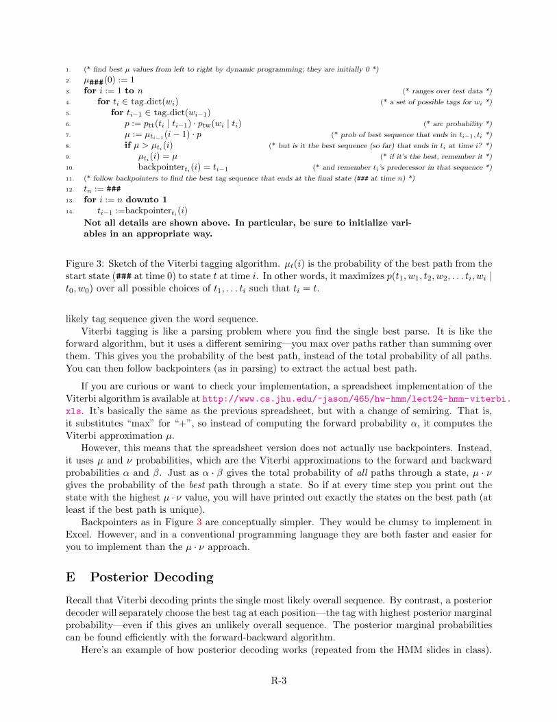
1. (* find best µ values from left to right by dynamic programming; they are initially 0 *)

2. µ###(0) := 13. for i := 1 to n (* ranges over test data *)

4. for ti ∈ tag dict(wi) (* a set of possible tags for wi *)

5. for ti−1 ∈ tag dict(wi−1)6. p := ptt(ti | ti−1) · ptw(wi | ti) (* arc probability *)

7. µ := µti−1(i− 1) · p (* prob of best sequence that ends in ti−1, ti *)

8. if µ > µti(i) (* but is it the best sequence (so far) that ends in ti at time i? *)

9. µti(i) = µ (* if it’s the best, remember it *)

10. backpointerti(i) = ti−1 (* and remember ti’s predecessor in that sequence *)

11. (* follow backpointers to find the best tag sequence that ends at the final state (### at time n) *)

12. tn := ###

13. for i := n downto 114. ti−1 :=backpointerti(i)

Not all details are shown above. In particular, be sure to initialize vari-ables in an appropriate way.

Figure 3: Sketch of the Viterbi tagging algorithm. µt(i) is the probability of the best path from thestart state (### at time 0) to state t at time i. In other words, it maximizes p(t1, w1, t2, w2, . . . ti, wi |t0, w0) over all possible choices of t1, . . . ti such that ti = t.

likely tag sequence given the word sequence.Viterbi tagging is like a parsing problem where you find the single best parse. It is like the

forward algorithm, but it uses a different semiring—you max over paths rather than summing overthem. This gives you the probability of the best path, instead of the total probability of all paths.You can then follow backpointers (as in parsing) to extract the actual best path.

If you are curious or want to check your implementation, a spreadsheet implementation of theViterbi algorithm is available at http://www.cs.jhu.edu/~jason/465/hw-hmm/lect24-hmm-viterbi.xls. It’s basically the same as the previous spreadsheet, but with a change of semiring. That is,it substitutes “max” for “+”, so instead of computing the forward probability α, it computes theViterbi approximation µ.

However, this means that the spreadsheet version does not actually use backpointers. Instead,it uses µ and ν probabilities, which are the Viterbi approximations to the forward and backwardprobabilities α and β. Just as α · β gives the total probability of all paths through a state, µ · νgives the probability of the best path through a state. So if at every time step you print out thestate with the highest µ · ν value, you will have printed out exactly the states on the best path (atleast if the best path is unique).

Backpointers as in Figure 3 are conceptually simpler. They would be clumsy to implement inExcel. However, and in a conventional programming language they are both faster and easier foryou to implement than the µ · ν approach.

E Posterior Decoding

Recall that Viterbi decoding prints the single most likely overall sequence. By contrast, a posteriordecoder will separately choose the best tag at each position—the tag with highest posterior marginalprobability—even if this gives an unlikely overall sequence. The posterior marginal probabilitiescan be found efficiently with the forward-backward algorithm.

Here’s an example of how posterior decoding works (repeated from the HMM slides in class).

R-3

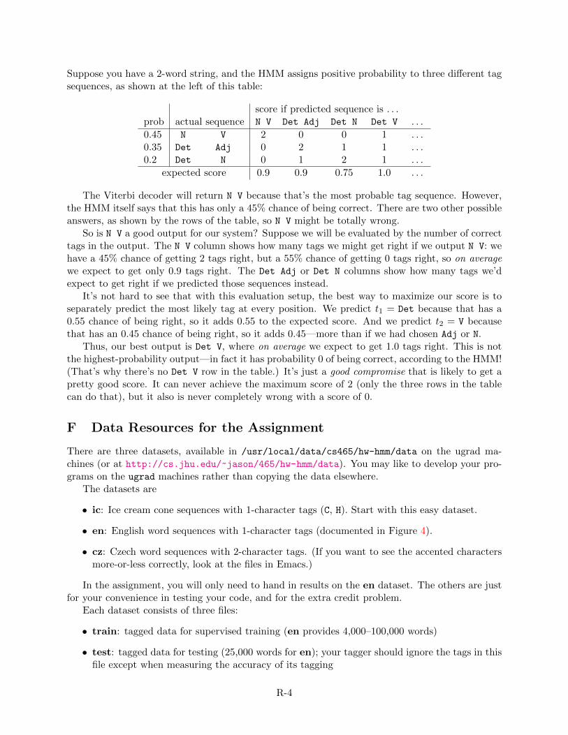
Suppose you have a 2-word string, and the HMM assigns positive probability to three different tagsequences, as shown at the left of this table:

score if predicted sequence is . . .prob actual sequence N V Det Adj Det N Det V . . .

0.45 N V 2 0 0 1 . . .0.35 Det Adj 0 2 1 1 . . .0.2 Det N 0 1 2 1 . . .

expected score 0.9 0.9 0.75 1.0 . . .

The Viterbi decoder will return N V because that’s the most probable tag sequence. However,the HMM itself says that this has only a 45% chance of being correct. There are two other possibleanswers, as shown by the rows of the table, so N V might be totally wrong.

So is N V a good output for our system? Suppose we will be evaluated by the number of correcttags in the output. The N V column shows how many tags we might get right if we output N V: wehave a 45% chance of getting 2 tags right, but a 55% chance of getting 0 tags right, so on averagewe expect to get only 0.9 tags right. The Det Adj or Det N columns show how many tags we’dexpect to get right if we predicted those sequences instead.

It’s not hard to see that with this evaluation setup, the best way to maximize our score is toseparately predict the most likely tag at every position. We predict t1 = Det because that has a0.55 chance of being right, so it adds 0.55 to the expected score. And we predict t2 = V becausethat has an 0.45 chance of being right, so it adds 0.45—more than if we had chosen Adj or N.

Thus, our best output is Det V, where on average we expect to get 1.0 tags right. This is notthe highest-probability output—in fact it has probability 0 of being correct, according to the HMM!(That’s why there’s no Det V row in the table.) It’s just a good compromise that is likely to get apretty good score. It can never achieve the maximum score of 2 (only the three rows in the tablecan do that), but it also is never completely wrong with a score of 0.

F Data Resources for the Assignment

There are three datasets, available in /usr/local/data/cs465/hw-hmm/data on the ugrad ma-chines (or at http://cs.jhu.edu/~jason/465/hw-hmm/data). You may like to develop your pro-grams on the ugrad machines rather than copying the data elsewhere.

The datasets are

• ic: Ice cream cone sequences with 1-character tags (C, H). Start with this easy dataset.

• en: English word sequences with 1-character tags (documented in Figure 4).

• cz: Czech word sequences with 2-character tags. (If you want to see the accented charactersmore-or-less correctly, look at the files in Emacs.)

In the assignment, you will only need to hand in results on the en dataset. The others are justfor your convenience in testing your code, and for the extra credit problem.

Each dataset consists of three files:

• train: tagged data for supervised training (en provides 4,000–100,000 words)

• test: tagged data for testing (25,000 words for en); your tagger should ignore the tags in thisfile except when measuring the accuracy of its tagging

R-4

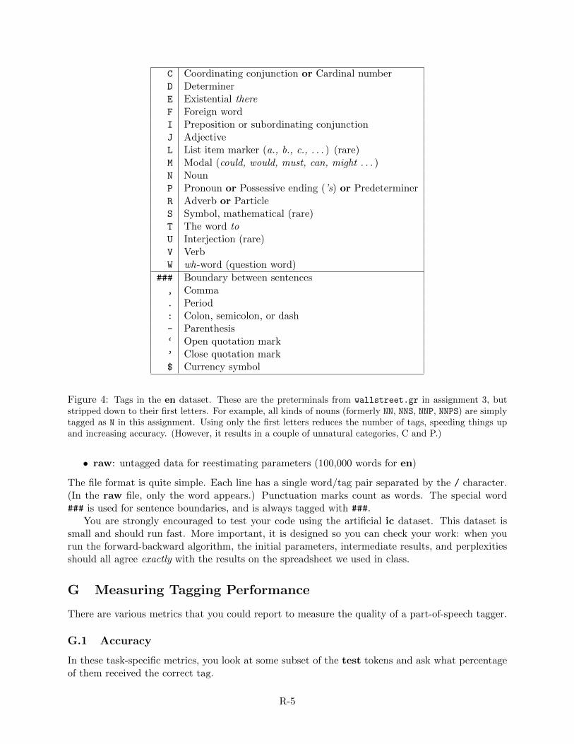
C Coordinating conjunction or Cardinal numberD DeterminerE Existential thereF Foreign wordI Preposition or subordinating conjunctionJ AdjectiveL List item marker (a., b., c., . . . ) (rare)M Modal (could, would, must, can, might . . . )N NounP Pronoun or Possessive ending (’s) or PredeterminerR Adverb or ParticleS Symbol, mathematical (rare)T The word toU Interjection (rare)V VerbW wh-word (question word)

### Boundary between sentences, Comma. Period: Colon, semicolon, or dash- Parenthesis‘ Open quotation mark’ Close quotation mark$ Currency symbol

Figure 4: Tags in the en dataset. These are the preterminals from wallstreet.gr in assignment 3, butstripped down to their first letters. For example, all kinds of nouns (formerly NN, NNS, NNP, NNPS) are simplytagged as N in this assignment. Using only the first letters reduces the number of tags, speeding things upand increasing accuracy. (However, it results in a couple of unnatural categories, C and P.)

• raw: untagged data for reestimating parameters (100,000 words for en)

The file format is quite simple. Each line has a single word/tag pair separated by the / character.(In the raw file, only the word appears.) Punctuation marks count as words. The special word### is used for sentence boundaries, and is always tagged with ###.

You are strongly encouraged to test your code using the artificial ic dataset. This dataset issmall and should run fast. More important, it is designed so you can check your work: when yourun the forward-backward algorithm, the initial parameters, intermediate results, and perplexitiesshould all agree exactly with the results on the spreadsheet we used in class.

G Measuring Tagging Performance

There are various metrics that you could report to measure the quality of a part-of-speech tagger.

G.1 Accuracy

In these task-specific metrics, you look at some subset of the test tokens and ask what percentageof them received the correct tag.

R-5

accuracy looks at all test tokens, except for the sentence boundary markers. (No one in NLP triesto take credit for tagging ### correctly with ###!)

known-word accuracy considers only tokens of words (other than ###) that also appeared intrain. So we have observed some possible parts of speech.

seen-word accuracy considers tokens of words that did not appear in train, but did appear inraw untagged data. Thus, we have observed the words in context and have used EM to tryto infer their parts of speech.

novel-word accuracy considers only tokens of words that did not appear in train or raw. Theseare very hard to tag, since context at test time is the only clue to the correct tag. But theyconstitute about 9% of all tokens in entest, so it is important to tag them as accurately aspossible.

vtagem’s output must also include the perplexity per untagged raw word. This is defined onraw data ~w as

exp

(− log p(w1, . . . wn | w0)

n

)Note that this does not mention the tags for raw data, which we don’t even know. It is easy tocompute, since you found Z = p(w1, . . . wn | w0) while running the forward-backward algorithm(Figure 2, line 8). It is the total probability of all paths (tag sequences compatible with thedictionary) that generate the raw word sequence.

G.2 Perplexity

As usual, perplexity is a useful task-independent metric that may correlate with accuracy.Given a tagged corpus, the model’s perplexity per tagged word is given by3

perplexity per tagged word = 2cross-entropy per tagged word (1)

where

cross-entropy per tagged word =− log2 p(w1, t1, . . . wn, tn | w0, t0)

n

Since the power of 2 and the log base 2 cancel each other out, you can equivalently write this usinga power of e and log base e:

perplexity per tagged word = exp (−log-likelihood per tagged word) (2)

= exp

(− log p(w1, t1, . . . wn, tn | w0, t0)

n

)(3)

This is equivalent because e−(log x)/n = (elog x)−1/n = x−1/n = (2log2 x)−1/n = 2−(log2 x)/n.Why is the corpus probability in the formula conditioned on w0, t0? Because you knew in

advance that the tagged test corpus would start with ###/###—your model is only predicting therest of that corpus. (The model has no parameter that would even tell you p(w0, t0). Instead,Figure 3, line 2, explicitly hard-codes your prior knowledge that t0 =###.)

3Using the notation from reading section B.

R-6

When you have untagged data, you can also compute the model’s perplexity on that:

perplexity per untagged word = exp (−log-likelihood per untagged word) (4)

= exp

(− log p(w1, . . . wn, | w0, t0)

n

)where the forward or backward algorithm can compute

p(w1, . . . wn, | w0, t0) =∑

t1,...,tn

p(w1, t1, . . . wn, tn | w0, t0) (5)

Notice that

p(w1, t1, . . . wn, tn | w0, t0) = p(w1, . . . wn | w0, t0) · p(t1, . . . tn | ~w, t0) (6)

so the tagged perplexity (2) can be regarded as the product of two perplexities—namely, howperplexed is the model by the words (in (4)), and how perplexed is it by the tags given the words?

To evaluate a trained model, you should ordinarily consider its perplexity on test data. Lowerperplexity is better.

On the other hand, models can be trained in the first place to minimize their perplexity on train-ing data. As equation (2), this is equivalent to maximizing the model’s likelihood (or log-likelihood)on training data. Maximizing the tagged likelihood p(w1, t1, . . . wn, tn | w0, t0) corresponds to un-smoothed training on a tagged corpus—as in question 2 on the assignment. Maximizing the un-tagged likelihood (5) corresponds to unsmoothed training on an untagged corpus, and is what EMattempts to do.

Thus, question 6 on the assignment will ask you to report (4) on untagged training data, simplyto track how well EM is improving its own training objective. This does not evaluate how well theresulting model will generalize to test data, which is why we will also ask you to report (2) on testdata.

H Implementation Hints for Viterbi Tagging

Make sure you really understand the algorithm before you start coding! Perhaps write pseudocodeor work out an example on paper. Review the reading or the slides. Coding should be a fewstraightforward hours of work if you really understand everything and can avoid careless bugs.

H.1 Steps of the Tagger

Your vtag program in the assignment should go through the following steps:

1. Read the train data and store the counts in global tables. (Your functions for computingprobabilities on demand, such as ptw, should access these tables. In problem 3, you willmodify those functions to do smoothing.)

2. Read the test data ~w into memory.

3. Follow the Viterbi algorithm pseudocode in Figure 3 to find the tag sequence ~t that maximizesp(~t, ~w).

4. Compute and print the accuracy and perplexity of the tagging. (You can compute the accu-racy at the same time as you extract the tag sequence while following backpointers.)

R-7

H.2 One Long String

Don’t bother to train on each sentence separately, or to tag each sentence separately. Just treatthe train file as one long string that happens to contain some ### words. Similarly for the testfile.

Tagging sentences separately would save you memory, since then you could throw away eachsentence (and its tag probabilities and backpointers) when you were done with it. But why botherif you seem to have enough memory? Just pretend it’s one long sentence. Worked for me.

H.3 Fixing the Vocabulary

As in homework 3, you should use the same vocabulary size V for all your computations, so thatyour perplexity results will be comparable to one another. So you need to compute it before youViterbi-tag test the first time (even though you have not used raw yet in any other way).

Take the vocabulary to be all the words that appeared at least once in train, plus an oov type.(Once you do EM, your vocabulary should also include the words that appeared at least once inraw.)

H.4 Data Structures

Some suggestions:

• Figure 3 refers to a “tag dictionary” that stores all the possible tags for each word. As longas you only use the ic dataset, the tag dictionary is so simple that you can specify it directlyin the code: tag dict(###) = {###}, and tag dict(w) = {C, H} for any other word w. But fornatural-language problems, you’ll generalize this as described in the assignment to derive thetag dictionary from training data.

• Before you start coding, make a list of the data structures you will need to maintain, andchoose names for those data structures as well as their access methods.

For example, you will have to look up certain values of c(· · · ). So write down, for example,that you will store the count c(ti−1, ti) in a table count tt whose elements have names likecount tt("D","N"). When you read the training data you will increment these elements.

• You will need some multidimensional tables, indexed by strings and/or integers, to store thetraining counts and the path probabilities. (E.g., count tt("D","N") above, and µD(5) inFigure 3.) There are various easy ways to implement these:

– a hash table indexed by a single string that happens to have two parts, such as "D/N"

or "5/D". This works well, and is especially memory-efficient since no space is wastedon nonexistent entries.

– a hash table of arrays. This wastes a little more space.

– an ordinary multidimensional array (or array of arrays). This means you have to convertstrings (words or tags) to integers and use those integers as array indices. But thisconversion is a simple matter of lookup in a hash table. (High-speed NLP packages doall their internal processing using integers, converting to and from strings only duringI/O.)

It’s best to avoid an array of hash tables or a hash table of hash tables. It is slow andwasteful of memory to have many small hash tables. Better to combine them into one bighash table as described in the first bullet point above.

R-8

H.5 Avoiding Underflow

Probabilities that might be small (such as α and β in Figure 2) should be stored in memory aslog-probabilities. Doing this is actually crucial to prevent underflow.4

• This handout has been talking in terms of probabilities, but when you see something likep := p · q you should implement it as something like lp = lp + log q, where lp is a variablestoring log p.

• Tricky question: If p is 0, what should you store in lp? How can you represent that valuein your program? You are welcome to use any trick or hack that works.5

• Suggestion: To simplify your code and avoid bugs, I recommend that you use log-probabilitiesrather than negative log-probabilities. Then you won’t have to remember to negate the outputto log or the input to exp. (The convention of negating log-probabilities is designed to keepminus signs out of the numbers; but when you’re coding, it’s safer to keep minus signs out ofthe formulas and code instead.)

Similarly, I recommend that you use natural logarithms (loge) because they are simpler thanlog2, slightly faster, and less prone to programming mistakes.

Yes, it’s conventional to report − log2 probabilities, (the unit here is “bits”). But you canstore loge x internally, and convert to bits only when and if you print it out: − log2 x =−(loge x)/ loge 2. (As it happens, you are not required to print any log-probabilities for thisassignment, only perplexities: see equation (3).

• The forward-backward algorithm requires you to add probabilities, as in p := p+ q. But youare probably storing these probabilities p and q as their logs, lp and lq.

You might try to write lp := log(exp lp+exp lq), but the exp operation will probably underflowand return 0—that is why you are using logs in the first place!

Instead you need to write lp := logsumexp(lp, lq), where

logsumexp(x, y)def=

{x+ log(1 + exp(y − x)) if y ≤ xy + log(1 + exp(x− y)) otherwise

You can check for yourself that this equals log(expx + exp y); that the exp can’t overflow(because its argument is always ≤ 0); and that you get an appropriate answer even if the expunderflows.

The sub-expression log(1+z) can be computed more quickly and accurately by the specializedfunction log1p(z) = z − z2/2 + z3/3 − · · · (Taylor series), which is usually available in themath library of your programming language (or see http://www.johndcook.com/cpp_log_

4At least, if you are tagging the test set as one long sentence (see above). Conceivably you might be able to getaway without logs if you are tagging one sentence at a time. That’s how the ice cream spreadsheet got away withoutusing logs: its corpus was only 33 “words.” There is also an alternative way to avoid logs, which you are welcome touse if you care to work out the details. It turns out that for most purposes you only care about the relative µ values(or α or β values) at each time step—i.e., up to a multiplicative constant. So to avoid underflow, you can rescalethem by an arbitrary constant at every time step, or every several time steps when they get too small.

5The IEEE floating-point standard does have a way of representing −∞, so you could genuinely set lp = -Inf,which will work correctly with +, >, and ≥. Or you could just use an extremely negative value. Or you could usesome other convention to represent the fact that p = 0, such as setting a boolean variable p is zero or setting lp tosome special value (e.g., lp = undef or lp = null in a language that supports this, or even lp = +9999, since a positivevalue like this will never be used to represent any other log-probability).

R-9

one_plus_x.html). This avoids ever computing 1+z, which would lose most of z’s significantdigits for small z.

Make sure to handle the special case where p = 0 or q = 0 (see above).

Tip: logsumexp is available in Python as numpy.logaddexp.

• If you want to be slick, you might consider implementing a Probability class for all of this.It should support binary operations *, +, and max. Also, it should have a constructor thatturns a real into a Probability, and a method for getting the real value of a Probability.

Internally, the Probability class stores p as log p, which enables it to represent very smallprobabilities. It has some other, special way of storing p = 0. The implementations of *, +,max need to pay attention to this special case.

You’re not required to write a class (or even to use an object-oriented language). You mayprefer just to inline these simple methods. But even so, the above is a good way of thinkingabout what you’re doing.

H.6 Counting Carefully

To be careful and obtain precisely the sample results provided in this assignment, your unigramcounts should skip the training file’s very first (or very last) ###/###.

So even though the training file appears to have n + 1 word/tag unigrams, you should onlycount n of these unigrams. This matches the fact that there are n bigrams.

This counting procedure also slightly affects c(t), c(w), and c(t, w).Why count this way? Because doing so makes the smoothed (or unsmoothed) probabilities sum

to 1 as required.The root of the problem is that there are n + 1 tagged words but only n tag-tag pairs. Omit-

ting one of the boundaries arranges that∑

t c(t),∑

w c(w), and∑

t,w c(t, w) all equal n, just as∑t,t′ c(t, t

′) = n.To see how this works out in practice, suppose you have the very short corpus

#/# H/3 C/2 #/# C/1 #/# (I’m abbreviating ### as # in this section)

I’m just saying that you should set c(#) = 2, not c(#) = 3, for both the tag # and the word #.Remember that probabilities have the form p(event | context). Let’s go through the settings wherec(#) is used:

• In an expression ptt(· | #), where we are transitioning from #. You want unsmoothed

ptt(H | #) = c(#H)

c(#)= 1

2 (not 13), because # only appears twice as a context (representing bos

at positions 0 and 3—the eos at position 5 is not the context for any event).

• In an expression ptt(# | ·), where we are transitioning to #. Now, unsmoothed ptt(# |C) = c(C#)

c(C) = 22 doesn’t use c(#). But it backs off to ptt(#), and you want unsmoothed

ptt(#) = c(#)n = 2

5 (not 35), because # only appears twice as an event (representing eos at

positions 3 and 5—the bos at position 0 is not an event but rather is given “for free” as thecontext of the first event, like the root symbol in a PCFG).

• In an expression ptw(# | #), where we are emitting a word from #. Reading section H.7notes that there’s no point in smoothing this probability or even estimating it from data: youknow it’s 1! But if you were to estimate it, you would want to count the unsmoothed value

R-10

c(##)

c(#)should be counted as 2

2 (not 33 , and certainly not 3

2). This is best interpreted as saying

that no word was ever emitted at position 0. The only thing that exists at position 0 is a bosstate that transitions to the H state.

When reestimating counts using raw data in problem 6, you should similarly ignore the initialor final ###/### in the raw data.

H.7 Don’t Guess When You Know

Don’t smooth ptw(wi = ### | ti = ###). This probability doesn’t have to be estimated from data.It should always be 1, because you know—without any data—that the ### tag always emits the### word.

Indeed, the only reason we even bother to specify ### words in the file, not just ### tags, isto make your code simpler and more uniform: “treat the file as one long string that happens tocontain some ### words.”

H.8 Checking Your Implementation

Check your implementation as follows. If you use add-1 smoothing without backoff, then vtag

ictrain ictest should yield a tagging accuracy of 87.88% or 90.91%,6 with no novel words anda perplexity per tagged test word of 4.326.7 If you turn smoothing off, then the correct resultsare shown in question 4 of the assignment, and you can use the Viterbi version of the spreadsheet(reading section D)—which doesn’t smooth—to check your µ probabilities and your tagging:

• ictrain has been designed so that your initial unsmoothed supervised training on it willyield the initial parameters from the spreadsheet (transition and emission probabilities).

• ictest has exactly the data from the spreadsheet. Running your Viterbi tagger with theabove parameters on ictest should produce the same values as the spreadsheet’s iteration 0:8

6Why are there two possibilities? Because the code in Figure 3 breaks ties arbitrarily. In this example, there aretwo tagging paths that disagree on day 27 but have exactly the same probability. So backpointerH(28) will be set toH or C according to how the tie is broken, which depends on whether t27 = H or t27 = C is considered first in the loopat line 5. (Since line 8 happens to be written with a strict inequality >, the tie will arbitrarily be broken in favor ofthe first one we try; the second one will not be strictly better and so will not be able to displace it. Using ≥ at line 8would instead break ties in favor of the last one we tried.)

As a result, you might get an output that agrees with either 29 or 30 of the “correct” tags given by ictest.Breaking ties arbitrarily is common practice. It’s so rare in real data for two floating-point numbers to be exactly ==

that the extra overhead of handling ties carefully probably isn’t worth it.Ideally, though, a Viterbi tagger would output both taggings in this unusual case, and give an average score of

29.5 correct tags. This is how you handled ties on HW3. However, keeping track of multiple answers is harder inthe Viterbi algorithm, when the answer is a whole sequence of tags. You would have to keep multiple backpointersat every point where you had a tie. Then the backpointers wouldn’t define a single best tag string, but rather, askinny FSA that weaves together all the tag strings that are tied for best. The output of the Viterbi algorithm wouldthen actually be this skinny FSA. (Or rather its reversal, so that the strings go right-to-left rather than left-to-right.)When I say it’s ”skinny,” I mean it is pretty close to a straight-line FSA, since it usually will only contain one or afew paths. To score this skinny FSA and give partial credit, you’d have to compute, for each tag, the fraction of itspaths that got the right answer on that tag. How would you do this efficiently? By running the forward-backwardalgorithm on the skinny FSA!

7A uniform probability distribution over the 7 possible tagged words (###/###, 1/C, 1/H, 2/C, 2/H, 3/C, 3/H) wouldgive a perplexity of 7, so 4.326 is an improvement.

8To check your work, you only have to look at iteration 0, at the left of the spreadsheet. But for your interest, thespreadsheet does do reestimation. It is just like the forward-backward spreadsheet, but uses the Viterbi approximation.Interestingly, this approximation prevents it from really learning the pattern in the ice cream data, especially when

R-11

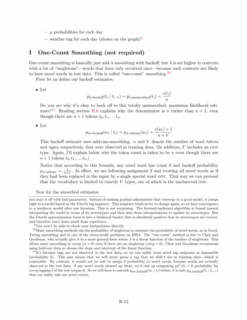
– µ probabilities for each day

– weather tag for each day (shown on the graph)9

I One-Count Smoothing (not required)

One-count smoothing is basically just add-λ smoothing with backoff, but λ is set higher in contextswith a lot of “singletons”—words that have only occurred once—because such contexts are likelyto have novel words in test data. This is called “one-count” smoothing.10

First let us define our backoff estimates:

• Let

ptt-backoff(ti | ti−1) = pt-unsmoothed(ti) =c(ti)

n

Do you see why it’s okay to back off to this totally unsmoothed, maximum likelihood esti-mate?11 Reading section H.6 explains why the denominator is n rather than n + 1, eventhough there are n+ 1 tokens t0, t1, . . . tn.

• Let

ptw-backoff(wi | ti) = pw-addone(wi) =c(wi) + 1

n+ V

This backoff estimate uses add-one-smoothing. n and V denote the number of word tokensand types, respectively, that were observed in training data. (In addition, V includes an oovtype. Again, I’ll explain below why the token count is taken to be n even though there aren+ 1 tokens t0, t1, . . . tn.)

Notice that according to this formula, any novel word has count 0 and backoff probabilitypw-addone = 1

n+V . In effect, we are following assignment 2 and treating all novel words as ifthey had been replaced in the input by a single special word oov. That way we can pretendthat the vocabulary is limited to exactly V types, one of which is the unobserved oov.

Now for the smoothed estimates:

you start it off with bad parameters. Instead of making gradual adjustments that converge to a good model, it jumpsright to a model based on the Viterbi tag sequence. This sequence tends never to change again, so we have convergenceto a mediocre model after one iteration. This is not surprising. The forward-backward algorithm is biased towardinterpreting the world in terms of its stereotypes and then uses those interpretations to update its stereotypes. Butthe Viterbi approximation turns it into a blinkered fanatic that is absolutely positive that its stereotypes are correct,and therefore can’t learn much from experience.

9You won’t be able to check your backpointers directly.10Many smoothing methods use the probability of singletons to estimate the probability of novel words, as in Good-

Turing smoothing and in one of the extra-credit problems on HW3. The “one-count” method is due to Chen andGoodman, who actually give it in a more general form where λ is a linear function of the number of singletons. Thisallows some smoothing to occur (λ > 0) even if there are no singletons (sing = 0). Chen and Goodman recommendusing held-out data to choose the slope and intercept of the linear function.

11It’s because tags are not observed in the test data, so we can safely treat novel tag unigrams as impossible(probability 0). This just means that we will never guess a tag that we didn’t see in training data—which isreasonable. By contrast, it would not be safe to assign 0 probability to novel words, because words are actuallyobserved in the test data: if any novel words showed up there, we’d end up computing p(~t, ~w) = 0 probability forevery tagging ~t of the test corpus ~w. So we will have to smooth ptw-backoff(wi | ti) below; it is only ptt-backoff(ti | ti−1)that can safely rule out novel events.

R-12

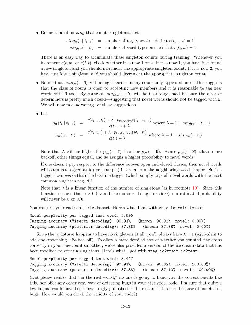
• Define a function sing that counts singletons. Let

singtt(· | ti−1) = number of tag types t such that c(ti−1, t) = 1

singtw(· | ti) = number of word types w such that c(ti, w) = 1

There is an easy way to accumulate these singleton counts during training. Whenever youincrement c(t, w) or c(t, t), check whether it is now 1 or 2. If it is now 1, you have just founda new singleton and you should increment the appropriate singleton count. If it is now 2, youhave just lost a singleton and you should decrement the appropriate singleton count.

• Notice that singtw(· | N) will be high because many nouns only appeared once. This suggeststhat the class of nouns is open to accepting new members and it is reasonable to tag newwords with N too. By contrast, singtw(· | D) will be 0 or very small because the class ofdeterminers is pretty much closed—suggesting that novel words should not be tagged with D.We will now take advantage of these suggestions.

• Let

ptt(ti | ti−1) =c(ti−1, ti) + λ · ptt-backoff(ti | ti−1)

c(ti−1) + λwhere λ = 1 + singtt(· | ti−1)

ptw(wi | ti) =c(ti, wi) + λ · ptw-backoff(wi | ti)

c(ti) + λwhere λ = 1 + singtw(· | ti)

Note that λ will be higher for ptw(· | N) than for ptw(· | D). Hence ptw(· | N) allows morebackoff, other things equal, and so assigns a higher probability to novel words.

If one doesn’t pay respect to the difference betwen open and closed classes, then novel wordswill often get tagged as D (for example) in order to make neighboring words happy. Such atagger does worse than the baseline tagger (which simply tags all novel words with the mostcommon singleton tag, N)!

Note that λ is a linear function of the number of singletons (as in footnote 10). Since thisfunction ensures that λ > 0 (even if the number of singletons is 0), our estimated probabilitywill never be 0 or 0/0.

You can test your code on the ic dataset. Here’s what I got with vtag ictrain ictest:

Model perplexity per tagged test word: 3.890

Tagging accuracy (Viterbi decoding): 90.91% (known: 90.91% novel: 0.00%)

Tagging accuracy (posterior decoding): 87.88% (known: 87.88% novel: 0.00%)

Since the ic dataset happens to have no singletons at all, you’ll always have λ = 1 (equivalent toadd-one smoothing with backoff). To allow a more detailed test of whether you counted singletonscorrectly in your one-count smoother, we’ve also provided a version of the ice cream data that hasbeen modified to contain singletons. Here’s what I got with vtag ic2train ic2test:

Model perplexity per tagged test word: 8.447

Tagging accuracy (Viterbi decoding): 90.91% (known: 90.32% novel: 100.00%)

Tagging accuracy (posterior decoding): 87.88% (known: 87.10% novel: 100.00%)

(But please realize that “in the real world,” no one is going to hand you the correct results likethis, nor offer any other easy way of detecting bugs in your statistical code. I’m sure that quite afew bogus results have been unwittingly published in the research literature because of undetectedbugs. How would you check the validity of your code?)

R-13

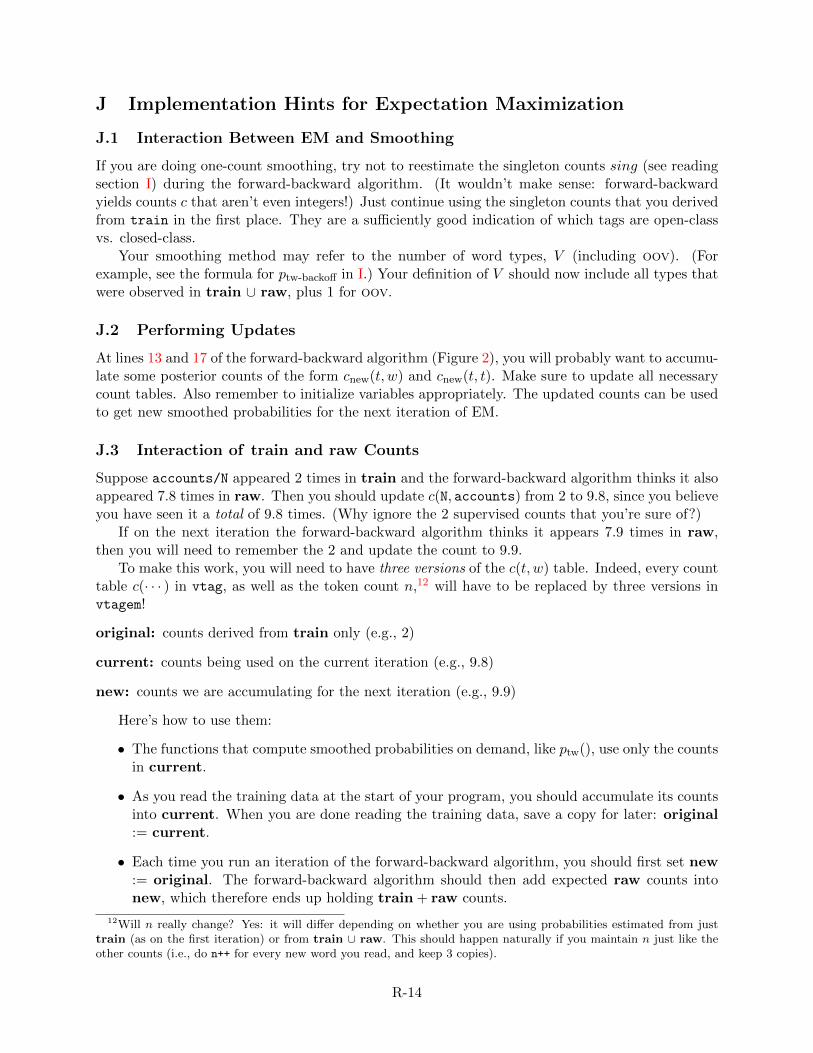
J Implementation Hints for Expectation Maximization

J.1 Interaction Between EM and Smoothing

If you are doing one-count smoothing, try not to reestimate the singleton counts sing (see readingsection I) during the forward-backward algorithm. (It wouldn’t make sense: forward-backwardyields counts c that aren’t even integers!) Just continue using the singleton counts that you derivedfrom train in the first place. They are a sufficiently good indication of which tags are open-classvs. closed-class.

Your smoothing method may refer to the number of word types, V (including oov). (Forexample, see the formula for ptw-backoff in I.) Your definition of V should now include all types thatwere observed in train ∪ raw, plus 1 for oov.

J.2 Performing Updates

At lines 13 and 17 of the forward-backward algorithm (Figure 2), you will probably want to accumu-late some posterior counts of the form cnew(t, w) and cnew(t, t). Make sure to update all necessarycount tables. Also remember to initialize variables appropriately. The updated counts can be usedto get new smoothed probabilities for the next iteration of EM.

J.3 Interaction of train and raw Counts

Suppose accounts/N appeared 2 times in train and the forward-backward algorithm thinks it alsoappeared 7.8 times in raw. Then you should update c(N, accounts) from 2 to 9.8, since you believeyou have seen it a total of 9.8 times. (Why ignore the 2 supervised counts that you’re sure of?)

If on the next iteration the forward-backward algorithm thinks it appears 7.9 times in raw,then you will need to remember the 2 and update the count to 9.9.

To make this work, you will need to have three versions of the c(t, w) table. Indeed, every counttable c(· · · ) in vtag, as well as the token count n,12 will have to be replaced by three versions invtagem!

original: counts derived from train only (e.g., 2)

current: counts being used on the current iteration (e.g., 9.8)

new: counts we are accumulating for the next iteration (e.g., 9.9)

Here’s how to use them:

• The functions that compute smoothed probabilities on demand, like ptw(), use only the countsin current.

• As you read the training data at the start of your program, you should accumulate its countsinto current. When you are done reading the training data, save a copy for later: original:= current.

• Each time you run an iteration of the forward-backward algorithm, you should first set new:= original. The forward-backward algorithm should then add expected raw counts intonew, which therefore ends up holding train + raw counts.

12Will n really change? Yes: it will differ depending on whether you are using probabilities estimated from justtrain (as on the first iteration) or from train ∪ raw. This should happen naturally if you maintain n just like theother counts (i.e., do n++ for every new word you read, and keep 3 copies).

R-14

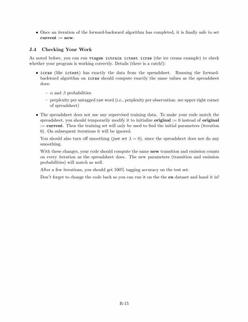
• Once an iteration of the forward-backward algorithm has completed, it is finally safe to setcurrent := new.

J.4 Checking Your Work

As noted before, you can run vtagem ictrain ictest icraw (the ice cream example) to checkwhether your program is working correctly. Details (there is a catch!):

• icraw (like ictest) has exactly the data from the spreadsheet. Running the forward-backward algorithm on icraw should compute exactly the same values as the spreadsheetdoes:

– α and β probabilities

– perplexity per untagged raw word (i.e., perplexity per observation: see upper right cornerof spreadsheet)

• The spreadsheet does not use any supervised training data. To make your code match thespreadsheet, you should temporarily modify it to initialize original := 0 instead of original:= current. Then the training set will only be used to find the initial parameters (iteration0). On subsequent iterations it will be ignored.

You should also turn off smoothing (just set λ = 0), since the spreadsheet does not do anysmoothing.

With these changes, your code should compute the same new transition and emission countson every iteration as the spreadsheet does. The new parameters (transition and emissionprobabilities) will match as well.

After a few iterations, you should get 100% tagging accuracy on the test set.

Don’t forget to change the code back so you can run it on the the en dataset and hand it in!

R-15