Embed Size (px)
Citation preview
6.006- Introduction to Algorithms6.006 Introduction to AlgorithmsLecture 19
Dynamic Programming IIProf Manolis KellisProf. Manolis Kellis
CLRS 15.4, 25.1, 25.2
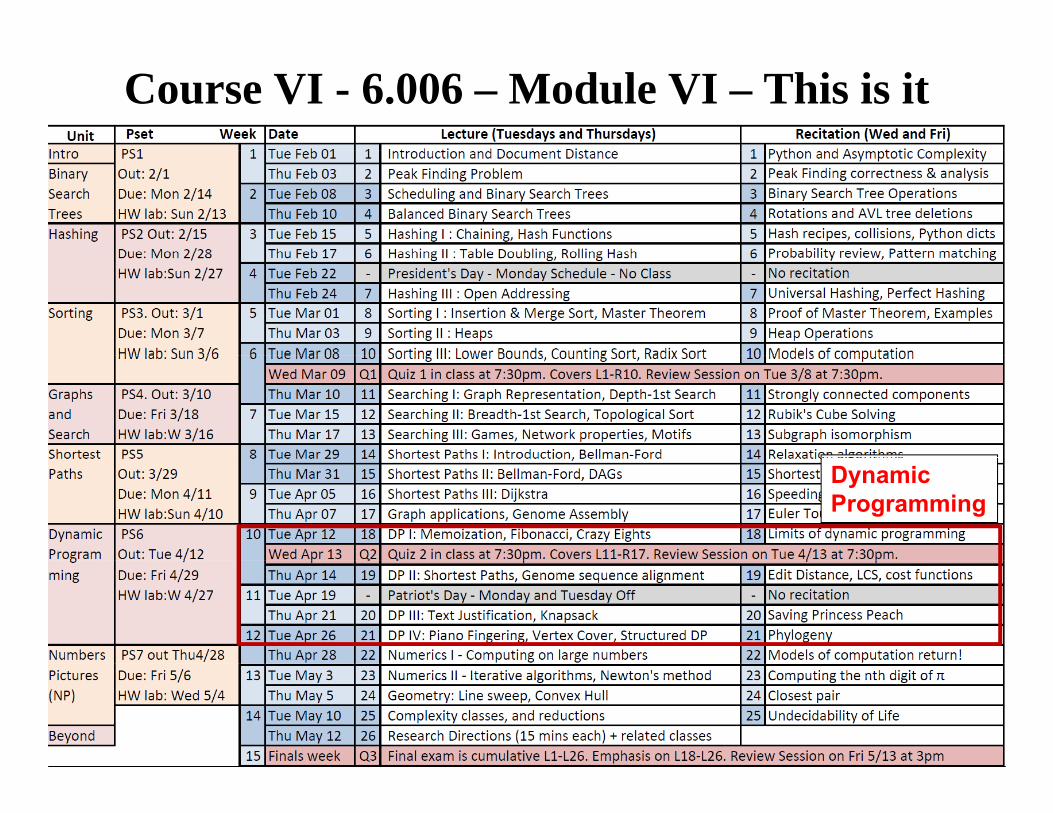
Course VI - 6.006 – Module VI – This is it
Dynamic Programming
2
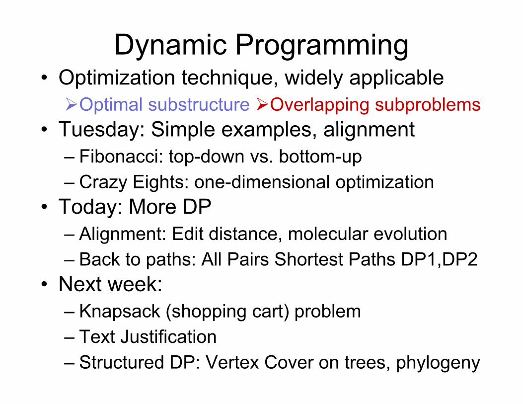
Dynamic Programming• Optimization technique widely applicable• Optimization technique, widely applicableOptimal substructure Overlapping subproblems
Tuesday: Simple examples alignment• Tuesday: Simple examples, alignment– Fibonacci: top-down vs. bottom-up
C Ei ht di i l ti i ti– Crazy Eights: one-dimensional optimization• Today: More DP
Ali t Edit di t l l l ti– Alignment: Edit distance, molecular evolution– Back to paths: All Pairs Shortest Paths DP1,DP2
N t k• Next week: – Knapsack (shopping cart) problem
f– Text Justification– Structured DP: Vertex Cover on trees, phylogeny
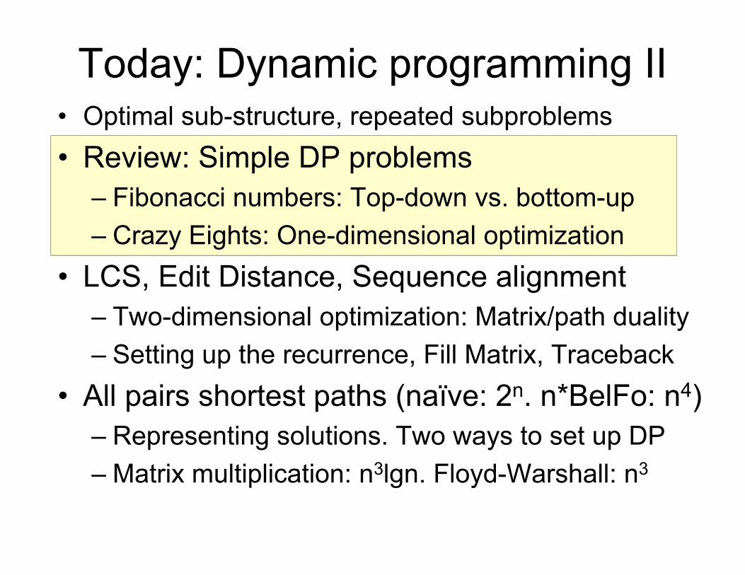
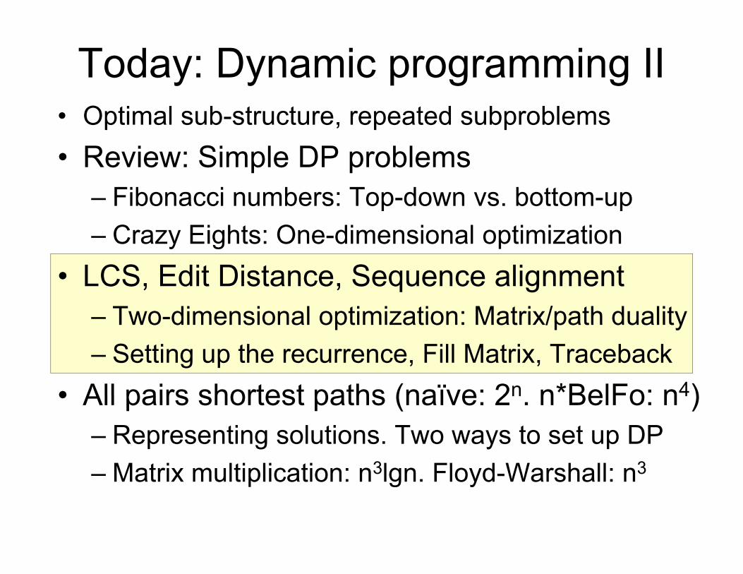
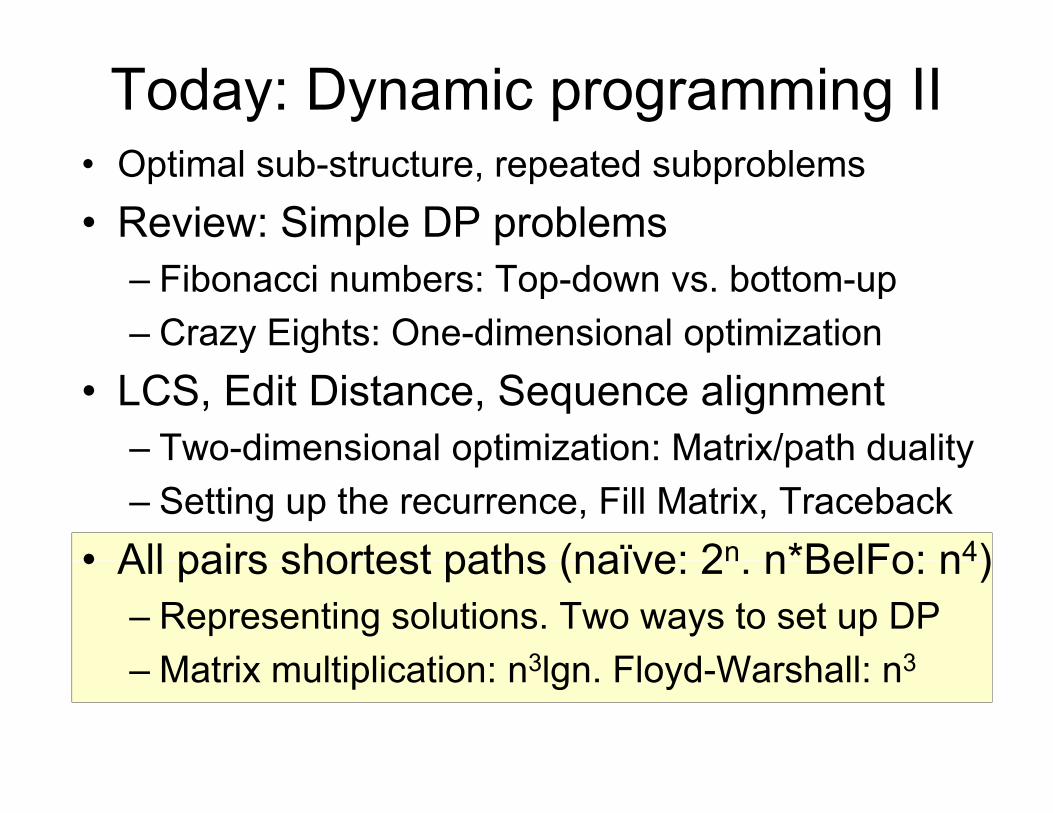
Today: Dynamic programming IIO i l b d b bl• Optimal sub-structure, repeated subproblems
• Review: Simple DP problems– Fibonacci numbers: Top-down vs. bottom-up– Crazy Eights: One-dimensional optimization
• LCS, Edit Distance, Sequence alignment– Two-dimensional optimization: Matrix/path dualityTwo dimensional optimization: Matrix/path duality– Setting up the recurrence, Fill Matrix, Traceback
• All pairs shortest paths (naïve: 2n n*BelFo: n4)• All pairs shortest paths (naïve: 2n. n BelFo: n4)– Representing solutions. Two ways to set up DP
Matrix multiplication: n3lgn Floyd Warshall: n3– Matrix multiplication: n3lgn. Floyd-Warshall: n3
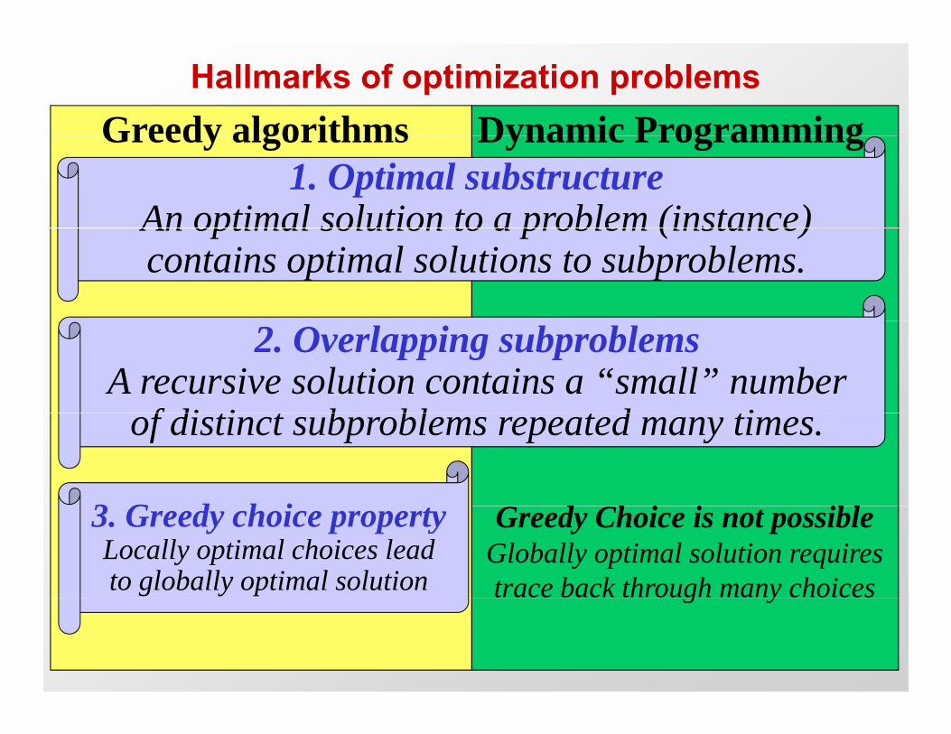
Hallmarks of optimization problemsGreedy algorithms Dynamic Programming
1. Optimal substructureAn optimal solution to a problem (instance)
Greedy algorithms Dynamic Programming
An optimal solution to a problem (instance) contains optimal solutions to subproblems.
2. Overlapping subproblemsA recursive solution contains a “small” number
f di ti t b bl t d tiof distinct subproblems repeated many times.
3 G d h i3. Greedy choice propertyLocally optimal choices lead to globally optimal solution
Greedy Choice is not possibleGlobally optimal solution requires trace back through many choicesg y
1 Fibonacci Computation1. Fibonacci Computation
(not really an optimization problem, but similar intuition applies))
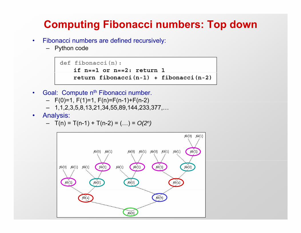
Computing Fibonacci numbers: Top down• Fibonacci numbers are defined recursively: y
– Python code
def fibonacci(n): if n==1 or n==2: return 1return fibonacci(n-1) + fibonacci(n-2)
• Goal: Compute nth Fibonacci number. – F(0)=1, F(1)=1, F(n)=F(n-1)+F(n-2)F(0) 1, F(1) 1, F(n) F(n 1) F(n 2)– 1,1,2,3,5,8,13,21,34,55,89,144,233,377,…
• Analysis: – T(n) = T(n-1) + T(n-2) = (…) = O(2n)
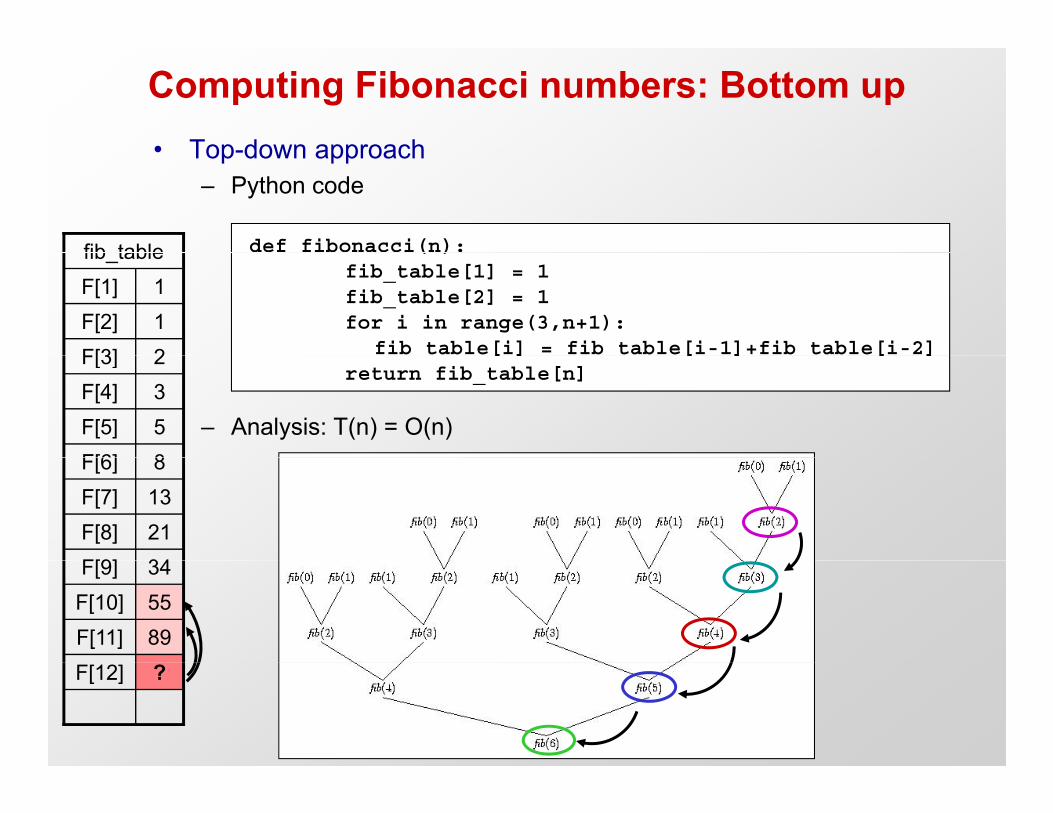
Computing Fibonacci numbers: Bottom up• Top-down approach• Top-down approach
– Python code
def fibonacci(n): fib table ( )fib_table[1] = 1fib_table[2] = 1for i in range(3,n+1):
fib table[i] = fib table[i-1]+fib table[i-2]2F[3]1F[2]1F[1]
fib_table
– Analysis: T(n) = O(n)
_ [ ] _ [ ] _ [ ]return fib_table[n]
8F[6]5F[5]3F[4]2F[3]
34F[9]21F[8]13F[7]8F[6]
89F[11]55F[10]34F[9]
?F[12]
2 Crazy Eights2. Crazy Eights
One-dimensional Optimization
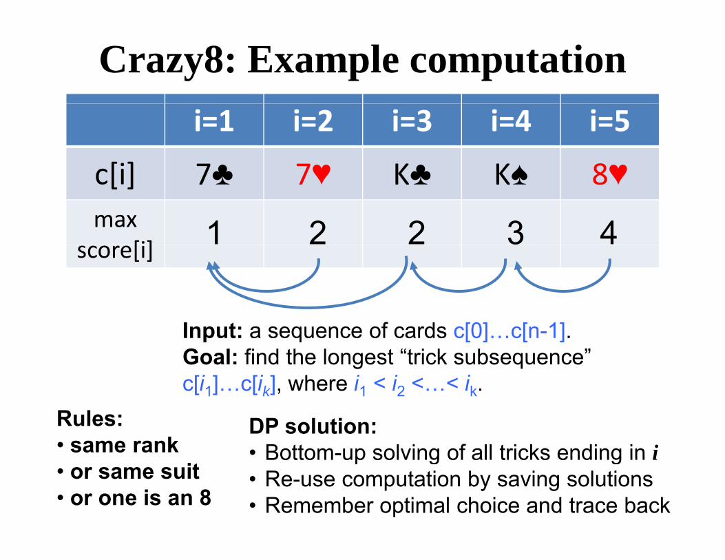
Crazy8: Example computationi=1 i=2 i=3 i=4 i=5
c[i] 7♣ 7♥ K♣ K♠ 8♥c[i] 7♣ 7♥ K♣ K♠ 8♥max
[i] 1 2 2 3 4score[i]
Input: a sequence of cards c[0]…c[n-1]. Goal: find the longest “trick subsequence” c[i1] c[ik] where i1 < i2 < < ik
Rules: • same rank
c[i1]…c[ik], where i1 < i2 <…< ik.
DP solution: • Bottom-up solving of all tricks ending in i
• or same suit • or one is an 8
Bottom up solving of all tricks ending in i• Re-use computation by saving solutions• Remember optimal choice and trace back
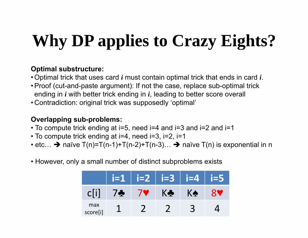
Why DP applies to Crazy Eights?Why DP applies to Crazy Eights?Optimal substructure: • Optimal trick that uses card i must contain optimal trick that ends in card i. • Proof (cut-and-paste argument): If not the case, replace sub-optimal trick ending in i with better trick ending in i, leading to better score overall
• Contradiction: original trick was supposedly ‘optimal’Contradiction: original trick was supposedly optimal
Overlapping sub-problems: • To compute trick ending at i=5, need i=4 and i=3 and i=2 and i=1
T t t i k di t i 4 d i 3 i 2 i 1• To compute trick ending at i=4, need i=3, i=2, i=1• etc… naïve T(n)=T(n-1)+T(n-2)+T(n-3)… naïve T(n) is exponential in n
• However, only a small number of distinct subproblems exists, y p
i=1 i=2 i=3 i=4 i=5c[i] 7♣ 7♥ K♣ K♠ 8♥c[i] 7♣ 7♥ K♣ K♠ 8♥max
score[i] 1 2 2 3 4
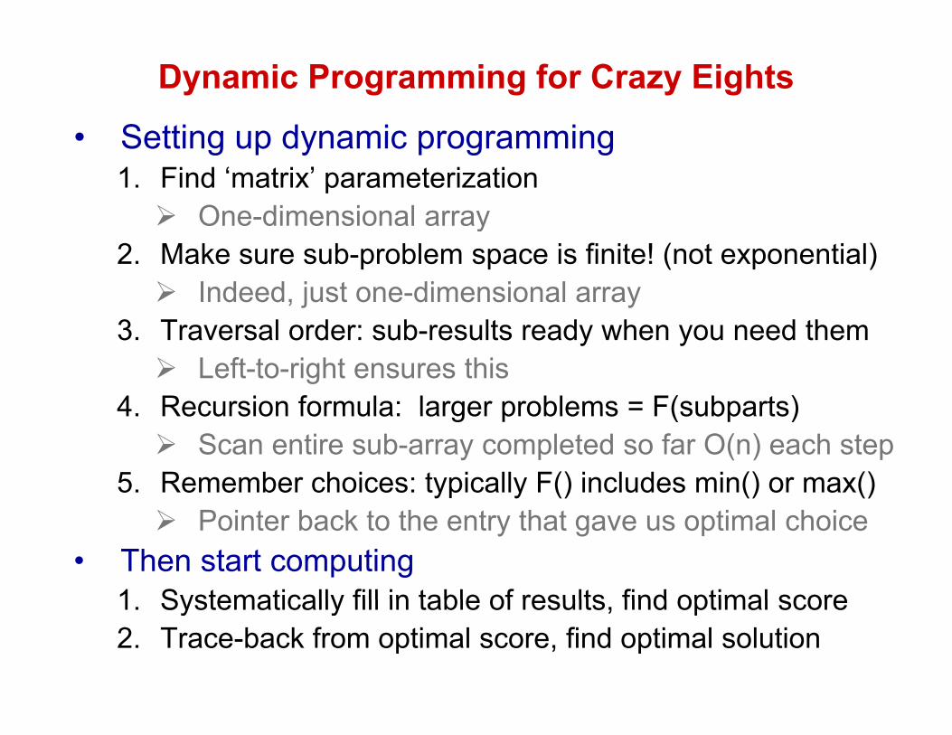
Dynamic Programming for Crazy Eights
• Setting up dynamic programming• Setting up dynamic programming1. Find ‘matrix’ parameterization One-dimensional arrayy
2. Make sure sub-problem space is finite! (not exponential) Indeed, just one-dimensional array
3 T l d b lt d h d th3. Traversal order: sub-results ready when you need them Left-to-right ensures this
4. Recursion formula: larger problems = F(subparts)4. Recursion formula: larger problems F(subparts) Scan entire sub-array completed so far O(n) each step
5. Remember choices: typically F() includes min() or max() Pointer back to the entry that gave us optimal choice
• Then start computing1 Systematically fill in table of results find optimal score1. Systematically fill in table of results, find optimal score2. Trace-back from optimal score, find optimal solution
Today: Dynamic programming IIO i l b d b bl• Optimal sub-structure, repeated subproblems
• Review: Simple DP problems– Fibonacci numbers: Top-down vs. bottom-up– Crazy Eights: One-dimensional optimization
• LCS, Edit Distance, Sequence alignment– Two-dimensional optimization: Matrix/path dualityTwo dimensional optimization: Matrix/path duality– Setting up the recurrence, Fill Matrix, Traceback
• All pairs shortest paths (naïve: 2n n*BelFo: n4)• All pairs shortest paths (naïve: 2n. n BelFo: n4)– Representing solutions. Two ways to set up DP
Matrix multiplication: n3lgn Floyd Warshall: n3– Matrix multiplication: n3lgn. Floyd-Warshall: n3
3. Sequence Alignment(aka Edit Distance aka LCS(aka. Edit Distance, aka. LCS,
Longest common subsequence)
T di i l ti i tiTwo-dimensional optimization
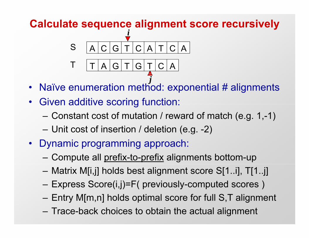
Calculate sequence alignment score recursively
S
i
A C G T C A T C A
T A G T G T C A
S
T
• Naïve enumeration method: exponential # alignments• Given additive scoring function:
j
Given additive scoring function:– Constant cost of mutation / reward of match (e.g. 1,-1)– Unit cost of insertion / deletion (e.g. -2)( g )
• Dynamic programming approach: – Compute all prefix-to-prefix alignments bottom-up– Matrix M[i,j] holds best alignment score S[1..i], T[1..j]– Express Score(i,j)=F( previously-computed scores )
E M[ ] h ld i l f f ll S T li– Entry M[m,n] holds optimal score for full S,T alignment– Trace-back choices to obtain the actual alignment
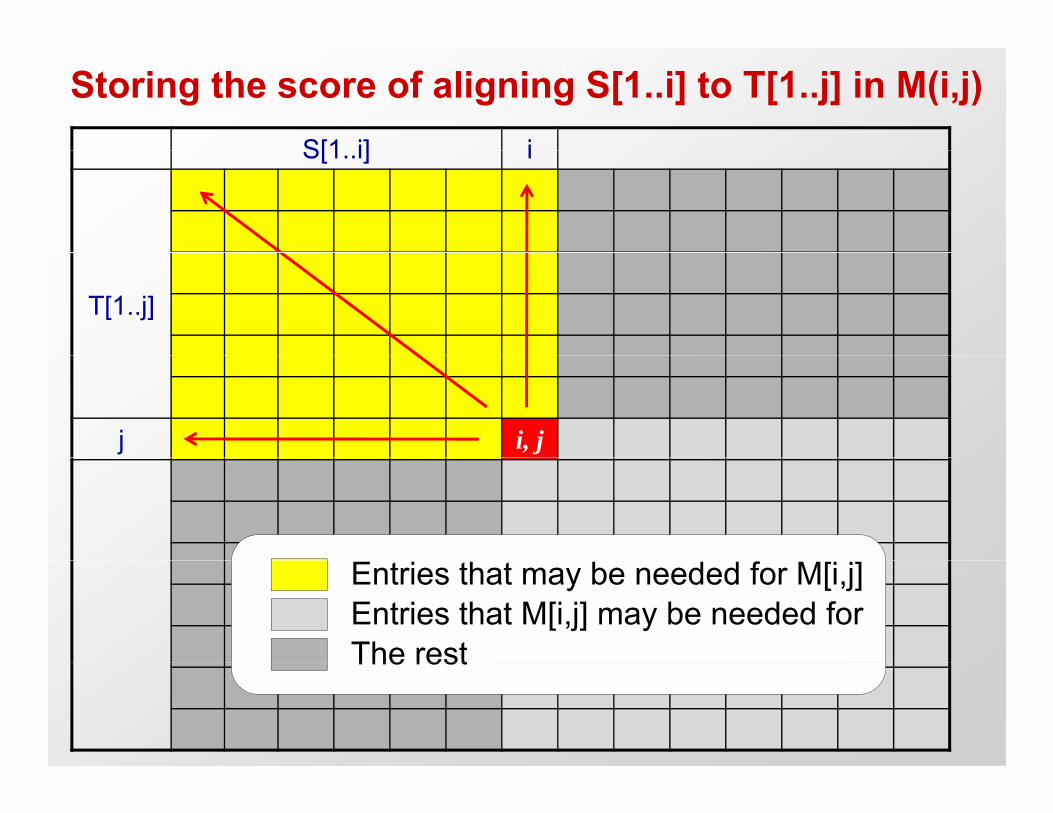
Storing the score of aligning S[1..i] to T[1..j] in M(i,j)S[1 i] iS[1..i] i
T[1..j]
j i, j
Entries that may be needed for M[i,j]Entries that M[i,j] may be needed forThe restThe rest
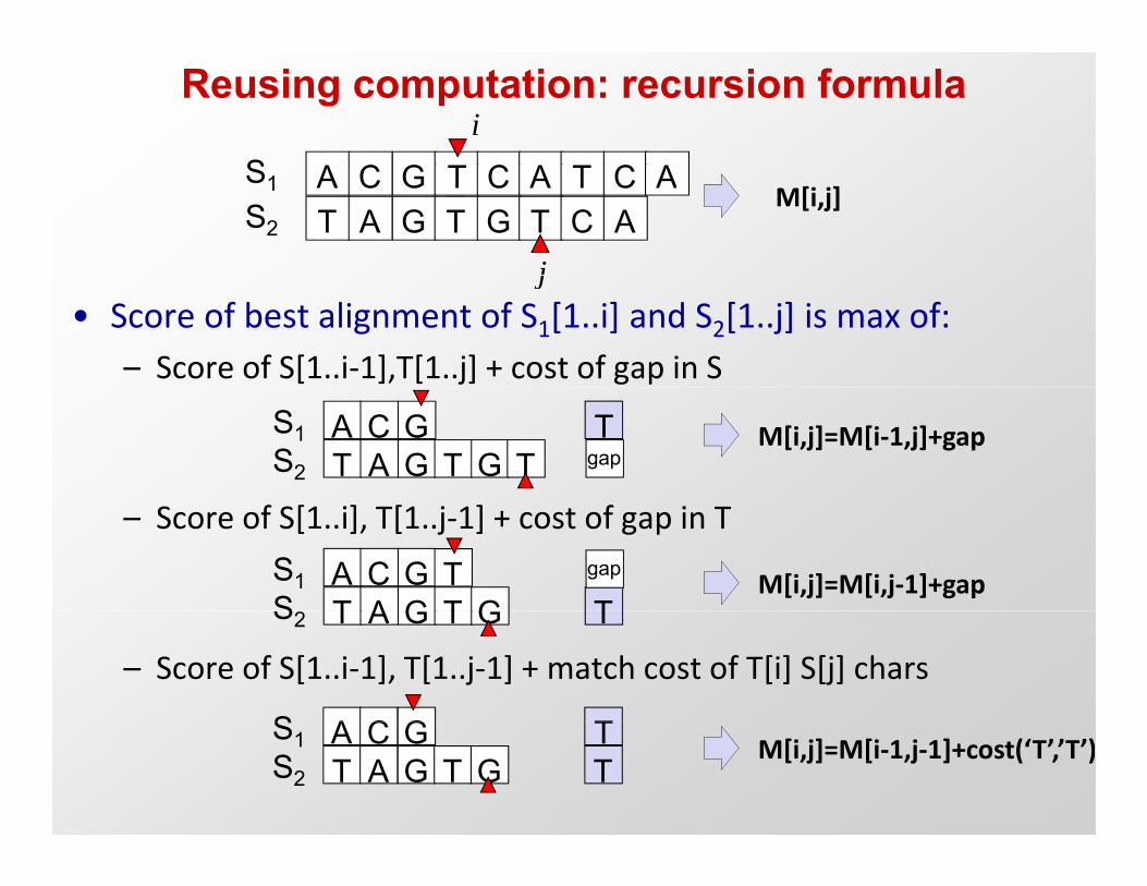
Reusing computation: recursion formula
Si
A C GT
CT A T C AT A G T G T C A
S1
S2
j
M[i,j]
• Score of best alignment of S1[1..i] and S2[1..j] is max of: – Score of S[1..i‐1],T[1..j] + cost of gap in S
j
M[i,j]=M[i‐1,j]+gapA C GT
TT A G T G T
S1S2
gap
– Score of S[1..i], T[1..j‐1] + cost of gap in T
M[i,j]=M[i,j‐1]+gapA C G TT A G T G T
S1S
gap
– Score of S[1..i‐1], T[1..j‐1] + match cost of T[i] S[j] chars
T A G T G TS2
A C G TSM[i,j]=M[i‐1,j‐1]+cost(‘T’,’T’)A C G T
T A G T G TS1S2
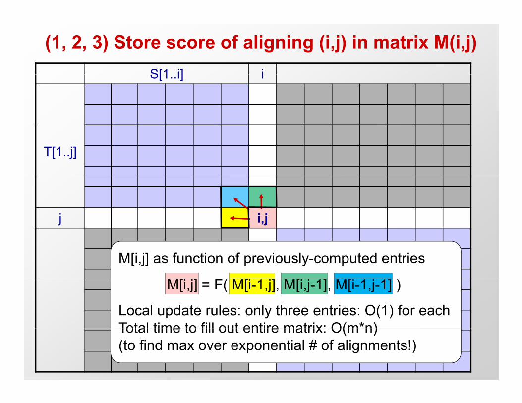
(1, 2, 3) Store score of aligning (i,j) in matrix M(i,j)S[1 i] iS[1..i] i
T[1..j]
j i,j
M[i,j] as function of previously-computed entries
Local update rules: only three entries: O(1) for eachTotal time to fill out entire matrix: O(m*n)
M[i,j] = F( M[i-1,j], M[i,j-1], M[i-1,j-1] )
Total time to fill out entire matrix: O(m n)(to find max over exponential # of alignments!)
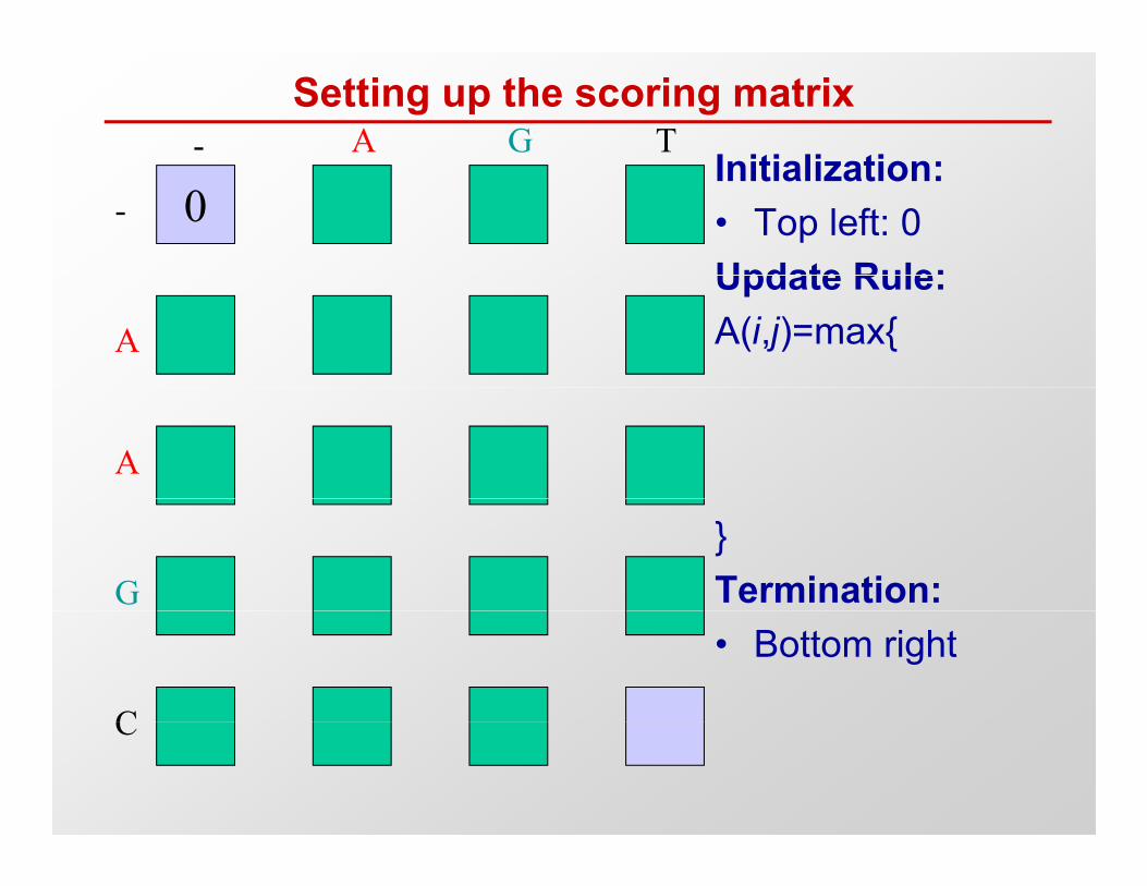
Setting up the scoring matrix- A G T
Initialization:- 0
Initialization:• Top left: 0Update Rule:
A
Update Rule:A(i,j)=max{
A
G}Termination:
C
• Bottom right
C
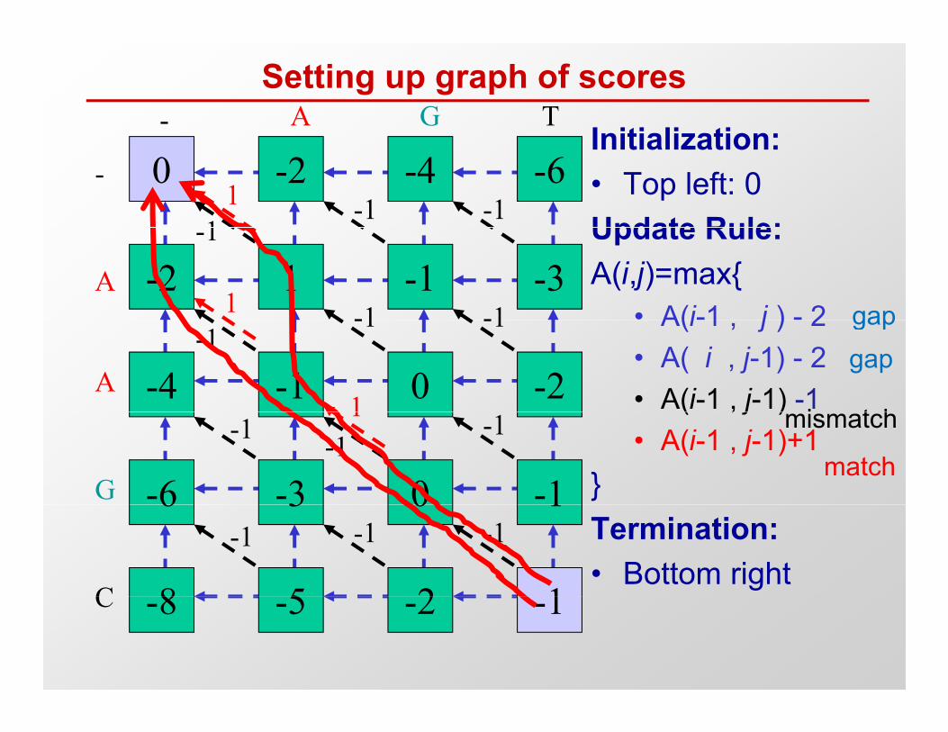
Setting up graph of scores- A G T
Initialization:- 0 -2 -4 -6
1-1 -1
Initialization:• Top left: 0Update Rule:
1
A -2 1 -1 -3-1
-1 -1
Update Rule:A(i,j)=max{
• A(i-1 j ) - 21 gap
A -4 -1 0 -2-1
-1 -1 A(i 1 , j ) 2• A( i , j-1) - 2• A(i-1 , j-1) -11 i t h
gapgap
G -6 -3 0 -1-1-1 -1
( , j )• A(i-1 , j-1)+1
}
1 mismatch
match
C
6 3 0 1
8 5 2 1
-1 -1 -1 Termination:• Bottom right
C -8 -5 -2 -1
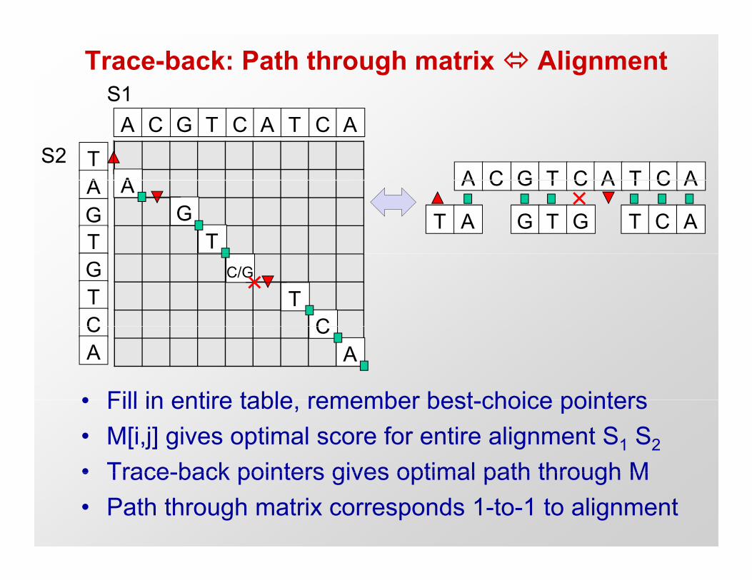
Trace-back: Path through matrix AlignmentS1
A C G T C A T C ATA
S2A C G T C A T C AAA
GT
A C G T C A T C A
T A G T G T C A
AG
TGTC
C/G
TC
• Fill in entire table remember best choice pointers
CA
CA
• Fill in entire table, remember best-choice pointers• M[i,j] gives optimal score for entire alignment S1 S2
• Trace-back pointers gives optimal path through M• Trace-back pointers gives optimal path through M• Path through matrix corresponds 1-to-1 to alignment
Dynamic Programming for sequence alignment
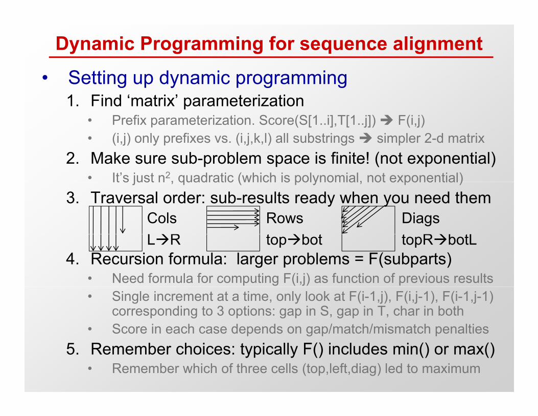
• Setting up dynamic programming• Setting up dynamic programming1. Find ‘matrix’ parameterization
• Prefix parameterization. Score(S[1..i],T[1..j]) F(i,j)• (i,j) only prefixes vs. (i,j,k,l) all substrings simpler 2-d matrix
2. Make sure sub-problem space is finite! (not exponential)• It’s just n2, quadratic (which is polynomial, not exponential)It s just n , quadratic (which is polynomial, not exponential)
3. Traversal order: sub-results ready when you need themColsLR
Rowst b t
Diagst Rb tL
4. Recursion formula: larger problems = F(subparts)• Need formula for computing F(i,j) as function of previous results
LR topbot topRbotL
• Single increment at a time, only look at F(i-1,j), F(i,j-1), F(i-1,j-1) corresponding to 3 options: gap in S, gap in T, char in both
• Score in each case depends on gap/match/mismatch penalties5. Remember choices: typically F() includes min() or max()
• Remember which of three cells (top,left,diag) led to maximum
Dynamic programming: design choices matter
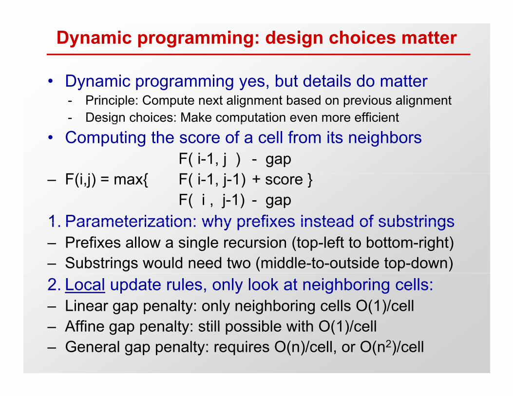
• Dynamic programming yes, but details do matter- Principle: Compute next alignment based on previous alignment- Design choices: Make computation even more efficientg p
• Computing the score of a cell from its neighborsF( i-1, j ) - gap
( ) { ( ) }– F(i,j) = max{ F( i-1, j-1) + score }F( i , j-1) - gap
1 Parameterization: why prefixes instead of substrings1. Parameterization: why prefixes instead of substrings– Prefixes allow a single recursion (top-left to bottom-right)– Substrings would need two (middle-to-outside top-down)2. Local update rules, only look at neighboring cells: – Linear gap penalty: only neighboring cells O(1)/cell
Affi lt till ibl ith O(1)/ ll– Affine gap penalty: still possible with O(1)/cell– General gap penalty: requires O(n)/cell, or O(n2)/cell
Today: Dynamic programming IIO i l b d b bl• Optimal sub-structure, repeated subproblems
• Review: Simple DP problems– Fibonacci numbers: Top-down vs. bottom-up– Crazy Eights: One-dimensional optimization
• LCS, Edit Distance, Sequence alignment– Two-dimensional optimization: Matrix/path dualityTwo dimensional optimization: Matrix/path duality– Setting up the recurrence, Fill Matrix, Traceback
• All pairs shortest paths (naïve: 2n n*BelFo: n4)• All pairs shortest paths (naïve: 2n. n BelFo: n4)– Representing solutions. Two ways to set up DP
Matrix multiplication: n3lgn Floyd Warshall: n3– Matrix multiplication: n3lgn. Floyd-Warshall: n3
All pairs shortest pathsAll pairs shortest paths
4. Matrix Multiplication5. Floyd-Warshall5. Floyd Warshall
April 14, 2011 L12.25
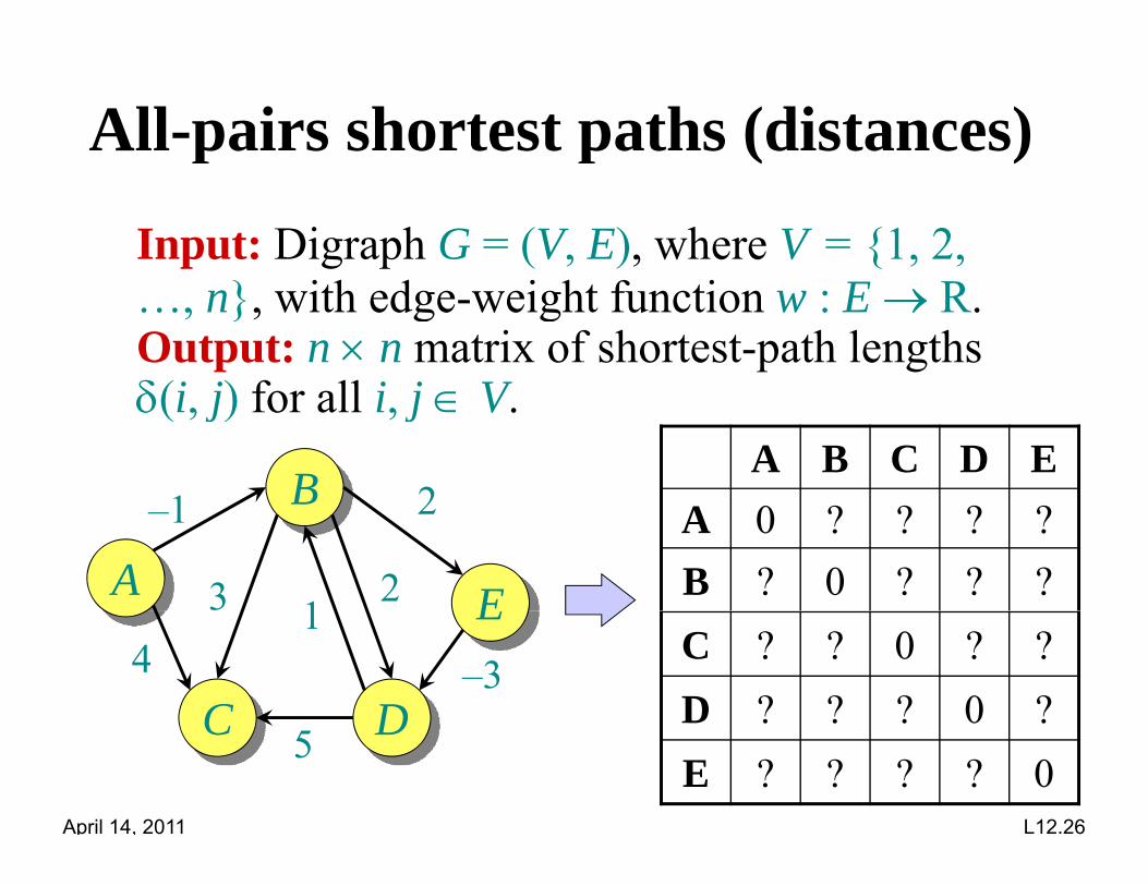
All-pairs shortest paths (distances)p p
Input: Digraph G = (V, E), where V = {1, 2, …, n}, with edge-weight function w : E R.Output: n n matrix of shortest-path lengths (i j) f ll i j V(i, j) for all i, j V.
B1 2A B C D E
A
B
E
–1
12
2
3
A 0 ? ? ? ?B ? 0 ? ? ?E
C D4
1–3
C ? ? 0 ? ?D ? ? ? 0 ?
April 14, 2011 L12.26
C D5D ? ? ? 0 ?E ? ? ? ? 0
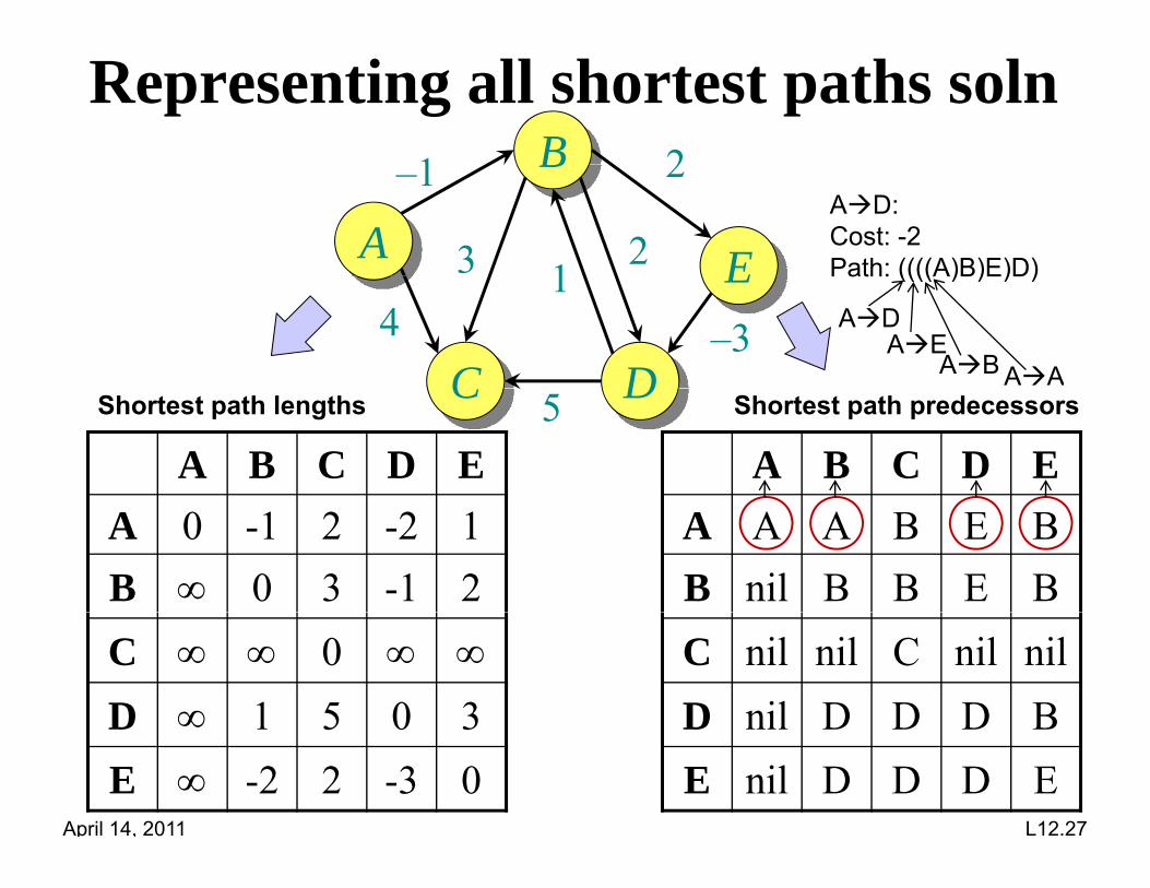
Representing all shortest paths solnB1 2
A
B
E
–1
12
2
3AD: Cost: -2Path: ((((A)B)E)D)E
C D4
1–3
Path: ((((A)B)E)D)
ADAE
AAABC D5A B C D EA B C D E
Shortest path lengths Shortest path predecessors
A A A B E BB nil B B E B
A 0 -1 2 -2 1B 0 3 -1 2
C nil nil C nil nilD nil D D D B
C 0
D 1 5 0 3
April 14, 2011 L12.27
D nil D D D BE nil D D D E
D 1 5 0 3E -2 2 -3 0
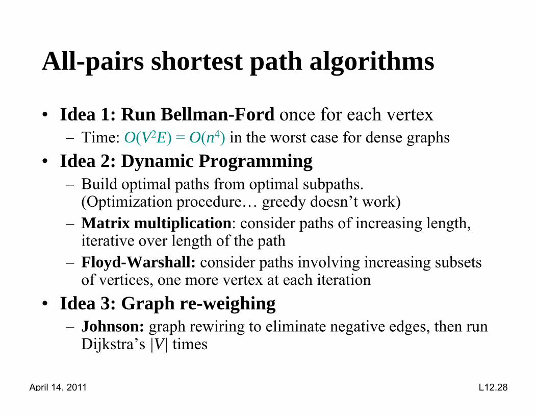
All-pairs shortest path algorithms
• Idea 1: Run Bellman-Ford once for each vertex– Time: O(V2E) = O(n4) in the worst case for dense graphs
• Idea 2: Dynamic ProgrammingB ild ti l th f ti l b th– Build optimal paths from optimal subpaths.(Optimization procedure… greedy doesn’t work)
– Matrix multiplication: consider paths of increasing length, iterative over length of the path
– Floyd-Warshall: consider paths involving increasing subsets of vertices, one more vertex at each iteration ,
• Idea 3: Graph re-weighing– Johnson: graph rewiring to eliminate negative edges, then run
Dijk ’ |V| i
April 14, 2011 L12.28
Dijkstra’s |V| times
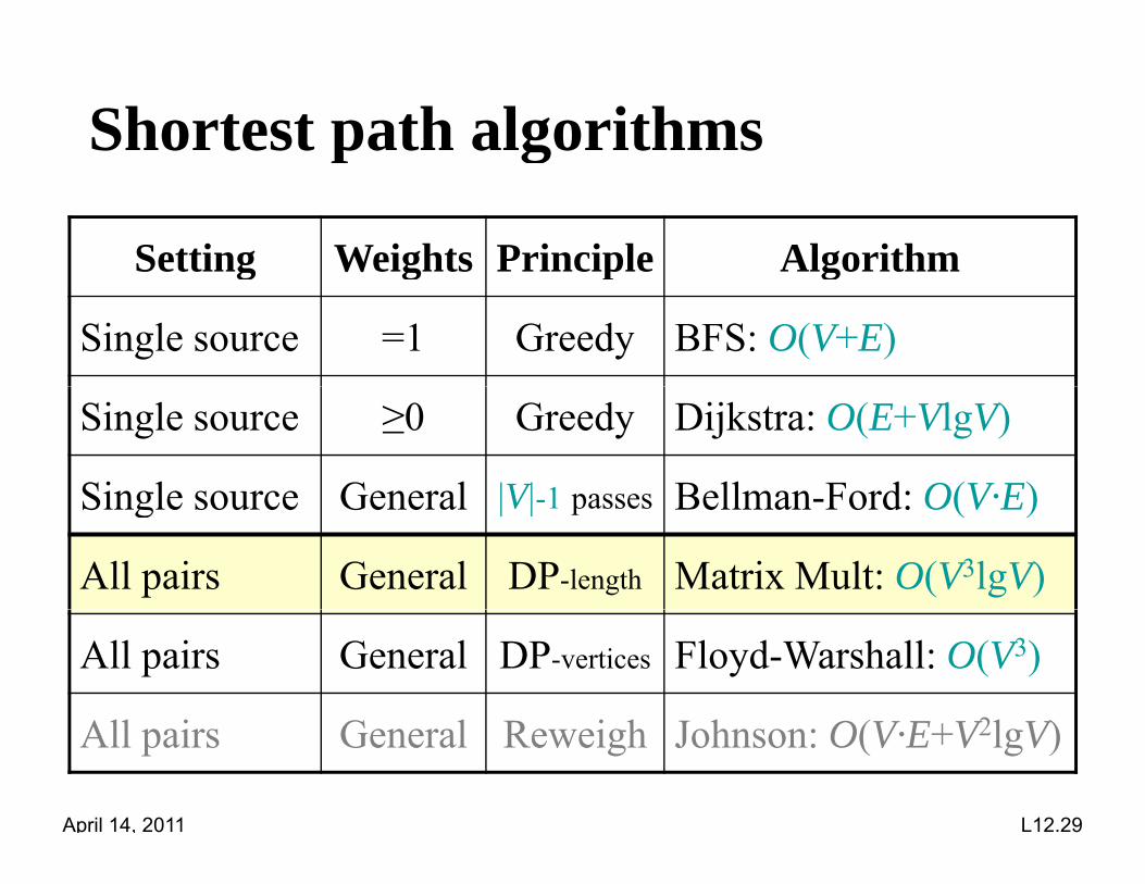
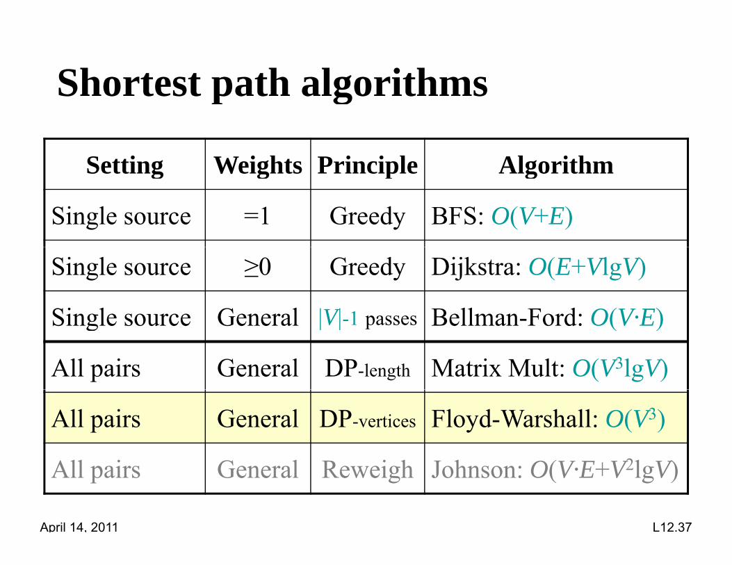
Shortest path algorithmsp g
Setting Weights Principle Algorithmg g p g
Single source =1 Greedy BFS: O(V+E)
Single source ≥0 Greedy Dijkstra: O(E+VlgV)
Single source General |V| 1 passes Bellman Ford: O(V·E)Single source General |V|-1 passes Bellman-Ford: O(V·E)
All pairs General DP-length Matrix Mult: O(V3lgV)
All pairs General DP-vertices Floyd-Warshall: O(V3)
All i G l R i h J h O(V E V2l V)
April 14, 2011 L12.29
All pairs General Reweigh Johnson: O(V·E+V2lgV)
4. Matrix Multiplication4. Matrix Multiplication
Consider paths of increasing lengthat each iteration
April 14, 2011 L12.30
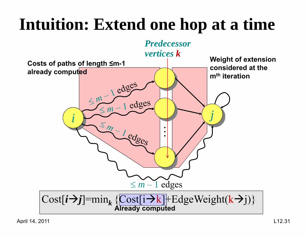
Intuition: Extend one hop at a timePredecessorPredecessorvertices k
Weight of extensionconsidered at the
th it ti
Costs of paths of length ≤m-1already computed mth iterationalready computed
i ji
m – 1 edges
April 14, 2011 L12.31
Cost[ij]=mink {Cost[ik]+EdgeWeight(kj)}Already computed
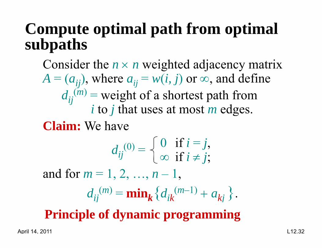
Compute optimal path from optimal subpathssubpaths
Consider the n n weighted adjacency matrix A = (a ) where a = w(i j) or and defineA = (aij), where aij = w(i, j) or , and define
dij(m) = weight of a shortest path from
i to j that uses at most m edges
0 if i jClaim: We have
i to j that uses at most m edges.
dij(0) = 0 if i = j,
if i j;d f 1 2 1and for m = 1, 2, …, n – 1,
dij(m) = mink{dik
(m–1) akj }.
April 14, 2011 L12.32
Principle of dynamic programming
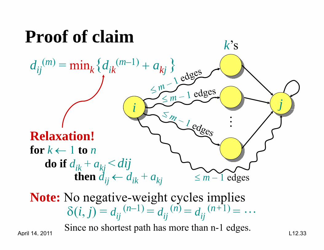
Proof of claim k’sdij
(m) = mink{dik(m–1) akj }
k s
i jii ji
Relaxation!for k 1 to n
do if dik + akj < dijd d m – 1 edges
jthen dij dik + akj
Note: No negative-weight cycles implies
April 14, 2011 L12.33
g g y p(i, j) = dij
(n–1) = dij (n) = dij
(n+1) = Since no shortest path has more than n-1 edges.
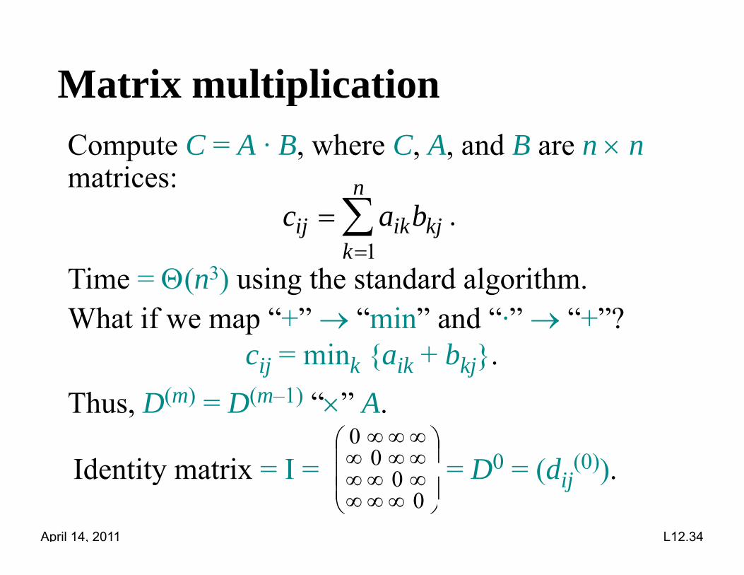
Matrix multiplicationpCompute C = A · B, where C, A, and B are n nmatrices:matrices:
n
kkjikij bac
1.
k 1Time = (n3) using the standard algorithm.What if we map “+” “min” and “·” “+”?What if we map + min and + ?
cij = mink {aik + bkj}.Th D(m) D(m 1) “ ” AThus, D(m) = D(m–1) “” A.
Identity matrix = I =
00
= D0 = (d (0))
April 14, 2011 L12.34
Identity matrix = I =
0
0 = D0 = (dij(0)).
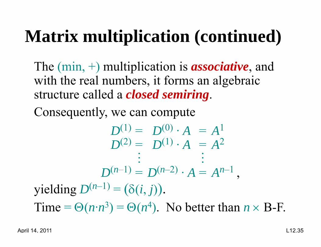
Matrix multiplication (continued)pThe (min, +) multiplication is associative, and
i h h l b i f l b iwith the real numbers, it forms an algebraic structure called a closed semiring.C lConsequently, we can compute
D(1) = D(0) · A = A1(2) (1) 2D(2) = D(1) · A = A2
D(n–1) D(n–2) A An–1D(n 1) = D(n 2) · A = An 1 ,
yielding D(n–1) = ((i, j)).
April 14, 2011 L12.35
Time = (n·n3) = (n4). No better than n B-F.
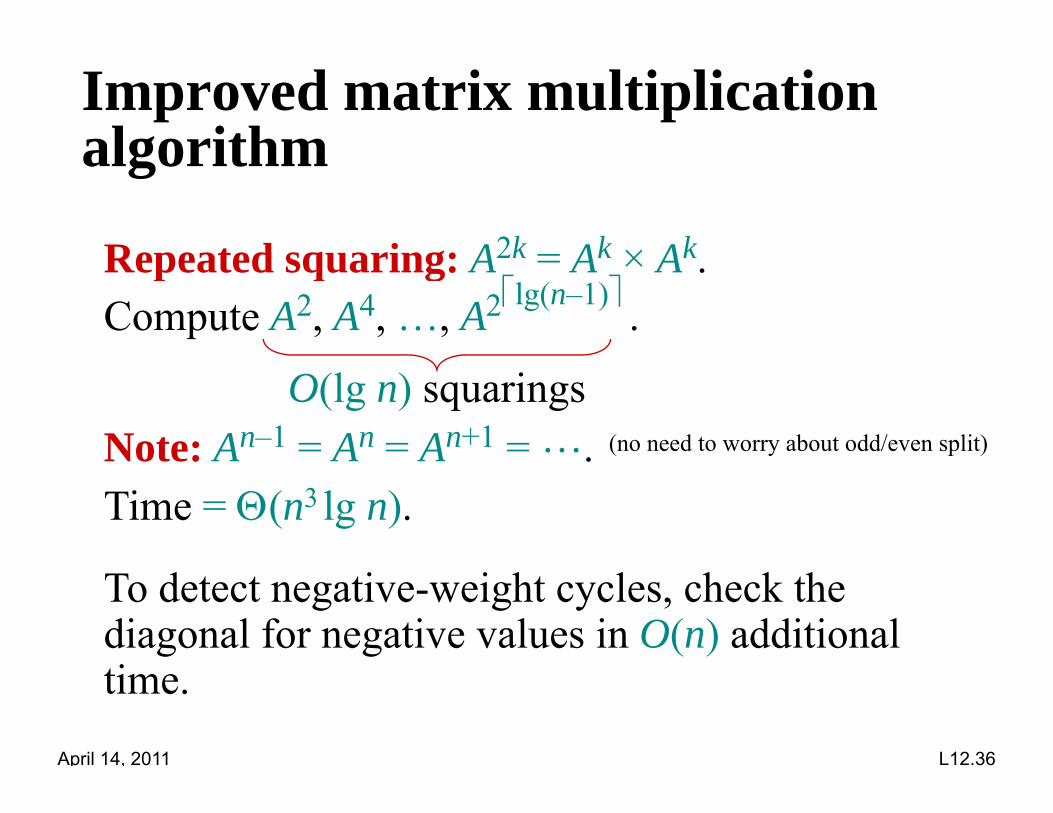
Improved matrix multiplication algorithmalgorithm
Repeated squaring: A2k Ak × AkRepeated squaring: A2k = Ak × Ak.Compute A2, A4, …, Alg(n–1) .
O(lg n) squaringsNote: An–1 = An = An+1 = . (no need to worry about odd/even split)
Time = (n3 lg n).Note: A A A .
To detect negative-weight cycles, check the diagonal for negative values in O(n) additional
April 14, 2011 L12.36
time.
Shortest path algorithmsp g
Setting Weights Principle Algorithmg g p g
Single source =1 Greedy BFS: O(V+E)
Single source ≥0 Greedy Dijkstra: O(E+VlgV)
Single source General |V| 1 passes Bellman Ford: O(V·E)Single source General |V|-1 passes Bellman-Ford: O(V·E)
All pairs General DP-length Matrix Mult: O(V3lgV)
All pairs General DP-vertices Floyd-Warshall: O(V3)
All i G l R i h J h O(V E V2l V)
April 14, 2011 L12.37
All pairs General Reweigh Johnson: O(V·E+V2lgV)
5. Floyd-Warshall algorithm5. Floyd Warshall algorithm
Consider one additional vertex each time
April 14, 2011 L12.38
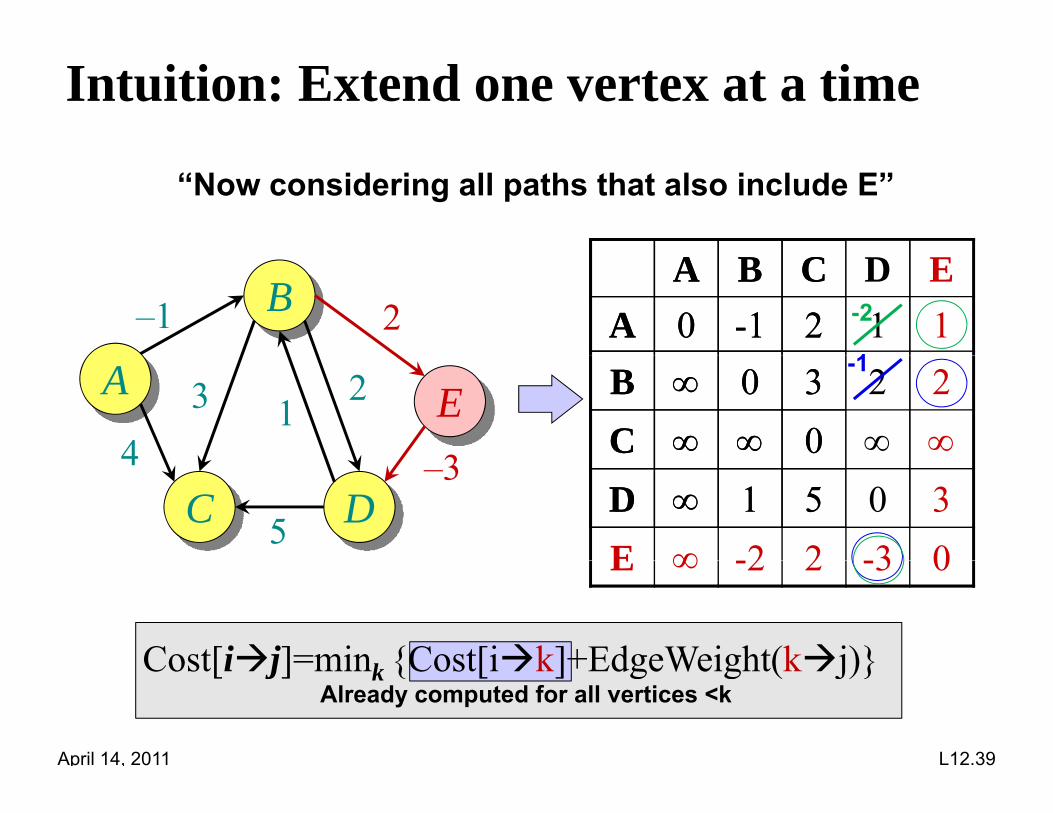
Intuition: Extend one vertex at a time
“Now considering all paths that also include E”
A B C DA 0 -1 2 1
A B C D EA 0 -1 2 1 1
B–1 21
-2
B 0 3 2C 0
B 0 3 2 2C 0
A
41
2 E3
3-1
D 1 5 0D 1 5 0 3E 2 2 3 0
C D4
5
–3
E -2 2 -3 0
Cost[ij]=min {Cost[ik]+EdgeWeight(kj)}
April 14, 2011 L12.39
Cost[ij] mink {Cost[ik]+EdgeWeight(kj)}Already computed for all vertices <k
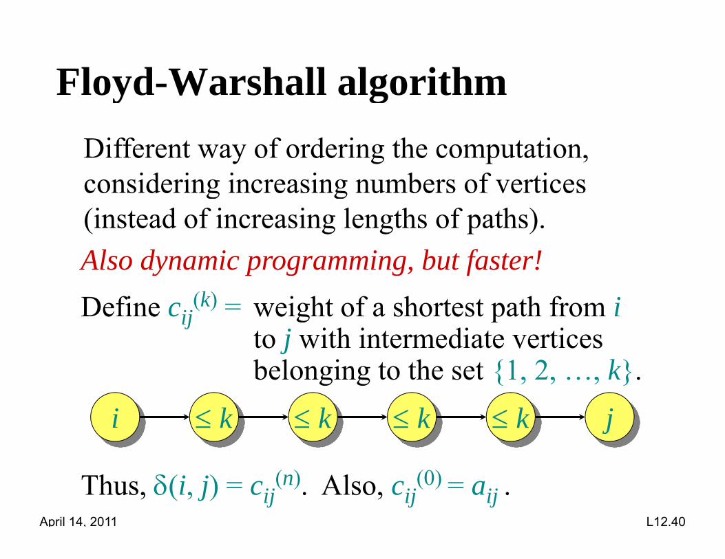
Floyd-Warshall algorithmy gDifferent way of ordering the computation,
id i i i b f iconsidering increasing numbers of vertices(instead of increasing lengths of paths).Also dynamic programming, but faster!Define cij
(k) = weight of a shortest path from iDefine cij weight of a shortest path from ito j with intermediate vertices belonging to the set {1, 2, …, k}.g g { }
i k k k k j
April 14, 2011 L12.40
Thus, (i, j) = cij(n). Also, cij
(0) = aij .
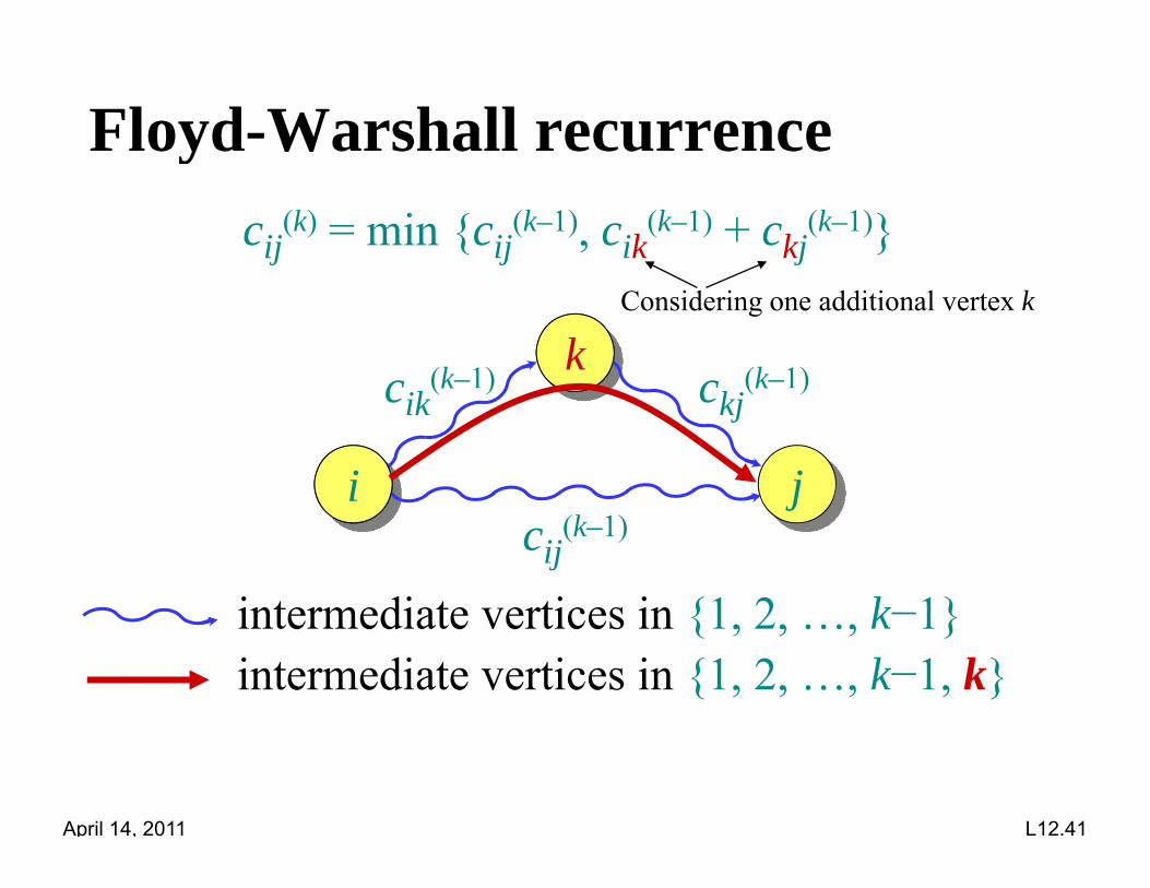
Floyd-Warshall recurrenceycij
(k) = min {cij(k–1), cik
(k–1) + ckj(k–1)}
kc (k–1) c (k–1)
Considering one additional vertex k
i ji
cik(k ) ckj
(k )
i jicij
(k–1)
intermediate vertices in {1 2 k 1}intermediate vertices in {1, 2, …, k−1}intermediate vertices in {1, 2, …, k−1, k}
April 14, 2011 L12.41
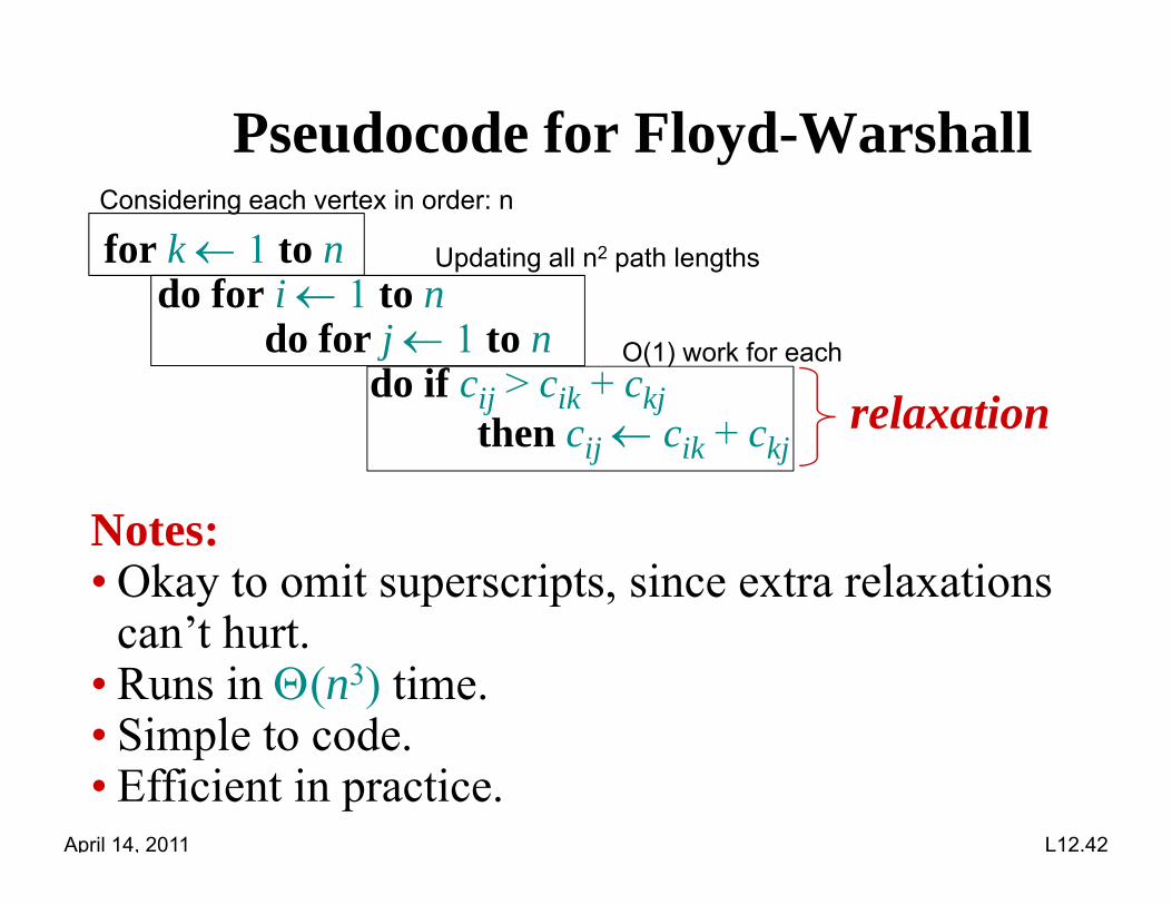
Pseudocode for Floyd-Warshall
for k 1 to nd f i 1 t
Considering each vertex in order: n
Updating all n2 path lengthsdo for i 1 to n
do for j 1 to ndo if cij > cik + ckj
O(1) work for eachdo if cij cik ckj
then cij cik + ckjrelaxation
Notes:• Okay to omit superscripts, since extra relaxations
’t h tcan’t hurt.• Runs in (n3) time.• Simple to code
April 14, 2011 L12.42
• Simple to code.• Efficient in practice.
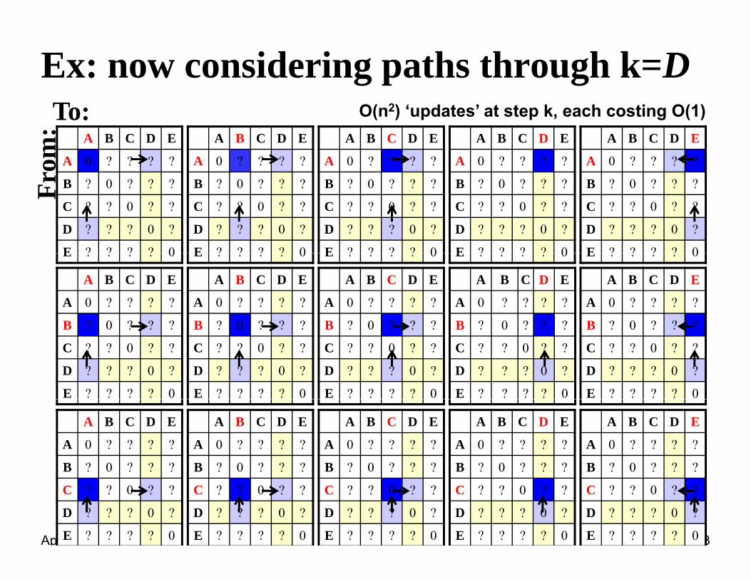
Ex: now considering paths through k=DT O( 2) ‘ d t ’ t t k h ti O(1)
A B C D E
A 0 ? ? ? ?
B ? 0 ? ? ?
A B C D E
A 0 ? ? ? ?
B ? 0 ? ? ?
A B C D E
A 0 ? ? ? ?
B ? 0 ? ? ?
A B C D E
A 0 ? ? ? ?
B ? 0 ? ? ?
A B C D E
A 0 ? ? ? ?
B ? 0 ? ? ?rom
:To: O(n2) ‘updates’ at step k, each costing O(1)
B ? 0 ? ? ?
C ? ? 0 ? ?
D ? ? ? 0 ?
E ? ? ? ? 0
B ? 0 ? ? ?
C ? ? 0 ? ?
D ? ? ? 0 ?
E ? ? ? ? 0
B ? 0 ? ? ?
C ? ? 0 ? ?
D ? ? ? 0 ?
E ? ? ? ? 0
B ? 0 ? ? ?
C ? ? 0 ? ?
D ? ? ? 0 ?
E ? ? ? ? 0
B ? 0 ? ? ?
C ? ? 0 ? ?
D ? ? ? 0 ?
E ? ? ? ? 0
Fr
E ? ? ? ? 0 E ? ? ? ? 0 E ? ? ? ? 0 E ? ? ? ? 0E ? ? ? ? 0
A B C D E
A 0 ? ? ? ?
B ? 0 ? ? ?
A B C D E
A 0 ? ? ? ?
B ? 0 ? ? ?
A B C D E
A 0 ? ? ? ?
B ? 0 ? ? ?
A B C D E
A 0 ? ? ? ?
B ? 0 ? ? ?
A B C D E
A 0 ? ? ? ?
B ? 0 ? ? ? B ? 0 ? ? ?
C ? ? 0 ? ?
D ? ? ? 0 ?
E ? ? ? ? 0
B ? 0 ? ? ?
C ? ? 0 ? ?
D ? ? ? 0 ?
E ? ? ? ? 0
B ? 0 ? ? ?
C ? ? 0 ? ?
D ? ? ? 0 ?
E ? ? ? ? 0
B ? 0 ? ? ?
C ? ? 0 ? ?
D ? ? ? 0 ?
E ? ? ? ? 0
B ? 0 ? ? ?
C ? ? 0 ? ?
D ? ? ? 0 ?
E ? ? ? ? 0
A B C D E
A 0 ? ? ? ?
B ? 0 ? ? ?
A B C D E
A 0 ? ? ? ?
B ? 0 ? ? ?
A B C D E
A 0 ? ? ? ?
B ? 0 ? ? ?
A B C D E
A 0 ? ? ? ?
B ? 0 ? ? ?
A B C D E
A 0 ? ? ? ?
B ? 0 ? ? ?
April 14, 2011 L12.43
C ? ? 0 ? ?
D ? ? ? 0 ?
E ? ? ? ? 0
C ? ? 0 ? ?
D ? ? ? 0 ?
E ? ? ? ? 0
C ? ? 0 ? ?
D ? ? ? 0 ?
E ? ? ? ? 0
C ? ? 0 ? ?
D ? ? ? 0 ?
E ? ? ? ? 0
C ? ? 0 ? ?
D ? ? ? 0 ?
E ? ? ? ? 0
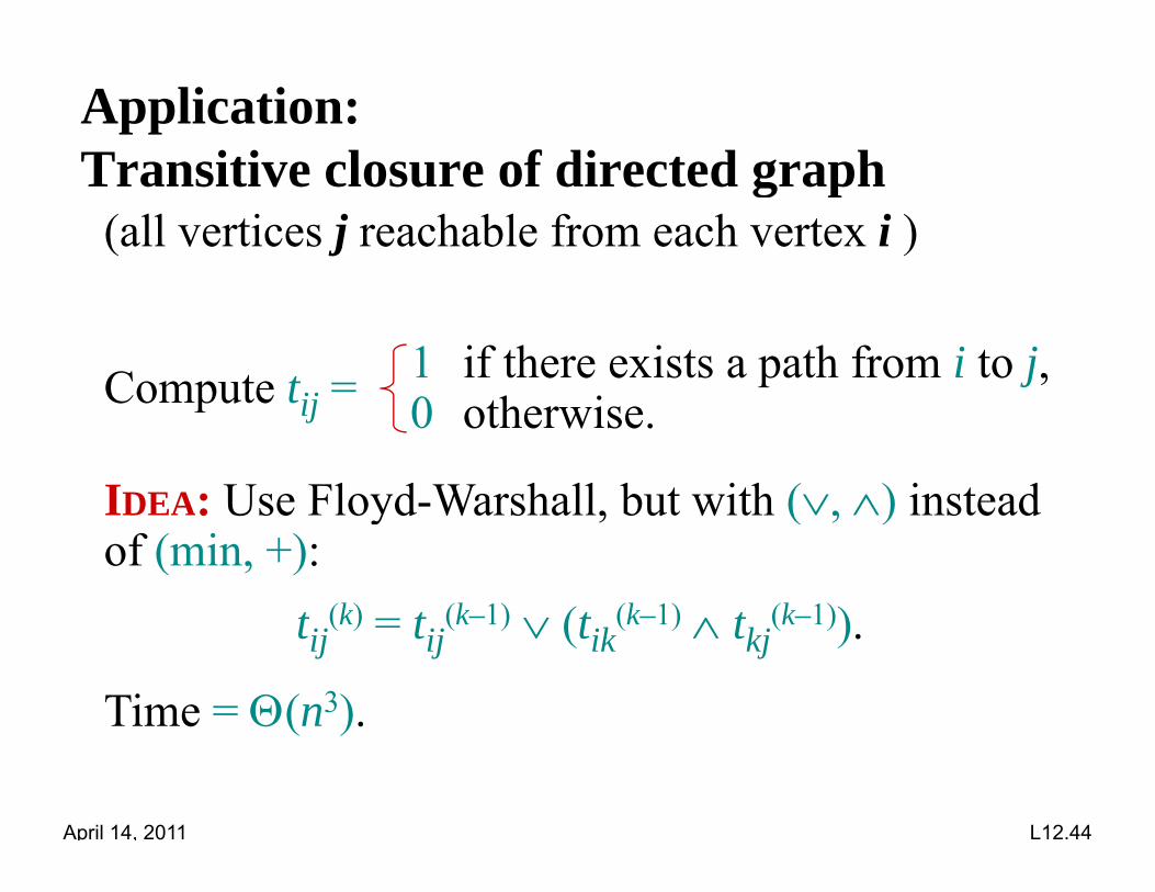
Application: Transitive closure of directed graphTransitive closure of directed graph
(all vertices j reachable from each vertex i )
Compute t = 1 if there exists a path from i to j,Compute tij = 0 otherwise.
IDEA: Use Floyd Warshall but with ( ) insteadIDEA: Use Floyd-Warshall, but with (, ) instead of (min, +):
t (k) t (k 1) (t (k 1) t (k 1))tij(k) = tij(k–1) (tik(k–1) tkj(k–1)).
Time = (n3).
April 14, 2011 L12.44
( )

Shortest path algorithmsp g
Setting Weights Principle Algorithmg g p g
Single source =1 Greedy BFS: O(V+E)
Single source ≥0 Greedy Dijkstra: O(E+VlgV)
Single source General |V| 1 passes Bellman Ford: O(V·E)Single source General |V|-1 passes Bellman-Ford: O(V·E)
All pairs General DP-length Matrix Mult: O(V3lgV)
All pairs General DP-vertices Floyd-Warshall: O(V3)
All i G l R i h J h O(V E V2l V)
April 14, 2011 L12.45
All pairs General Reweigh Johnson: O(V·E+V2lgV)
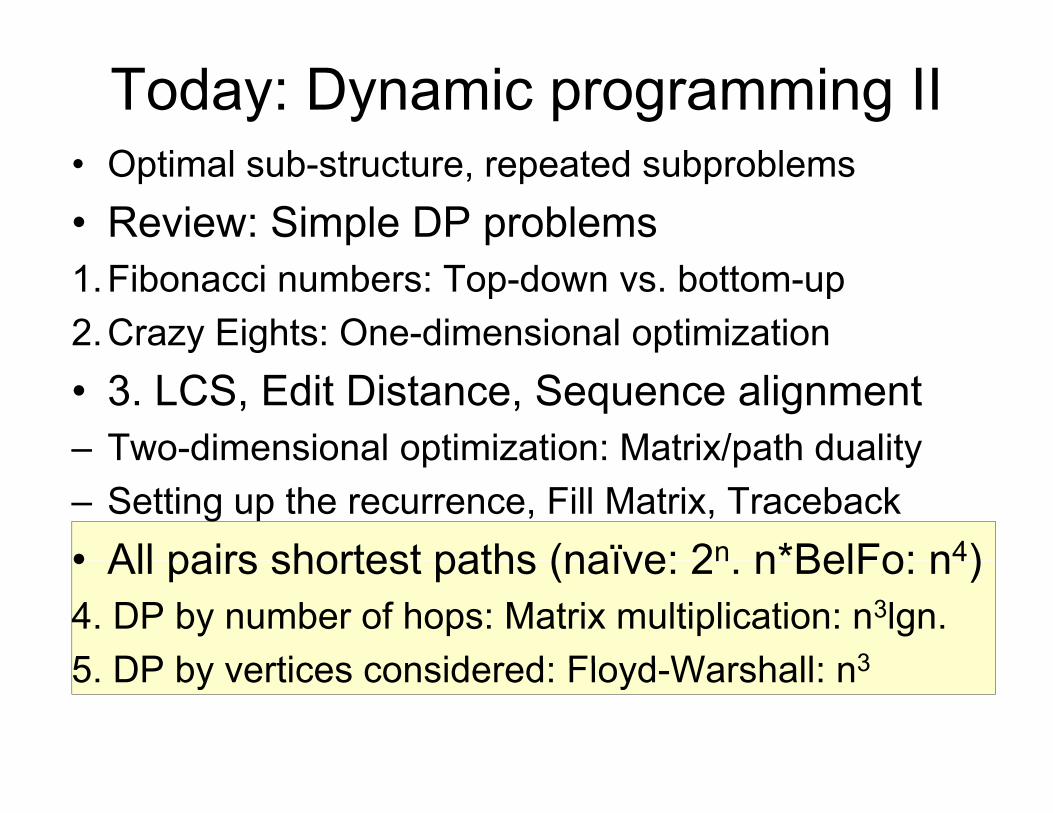
Today: Dynamic programming IIO i l b d b bl• Optimal sub-structure, repeated subproblems
• Review: Simple DP problems1.Fibonacci numbers: Top-down vs. bottom-up2.Crazy Eights: One-dimensional optimization• 3. LCS, Edit Distance, Sequence alignment– Two-dimensional optimization: Matrix/path dualityTwo dimensional optimization: Matrix/path duality– Setting up the recurrence, Fill Matrix, Traceback• All pairs shortest paths (naïve: 2n n*BelFo: n4)• All pairs shortest paths (naïve: 2n. n BelFo: n4)4. DP by number of hops: Matrix multiplication: n3lgn. 5 DP by vertices considered: Floyd Warshall: n35. DP by vertices considered: Floyd-Warshall: n3
Dynamic Programming module• Optimization technique widely applicable• Optimization technique, widely applicableOptimal substructure Overlapping subproblems
Tuesday: Simple examples alignment• Tuesday: Simple examples, alignment– Simple examples: Fibonacci, Crazy Eights
Ali t Edit di t l l l ti– Alignment: Edit distance, molecular evolution• Today: More DP
Ali t B d Li S Affi G– Alignment: Bound, Linear Space, Affine Gaps– Back to paths: All Pairs Shortest Paths DP1,DP2
N t k• Next week: – Knapsack (shopping cart) problem
f– Text Justification– Structured DP: Vertex Cover on trees, phylogeny

Happy Patriot’s Day!
Dynamic Programming
48