6 Week 3. Fama-French and the cross section of stock returns —

detailed notes

1. Big questions.

(a) Last week — does expected return vary over time? Is1999(2000) different from2004(

2005)?

If so, why? (Something about higher risk premium in recessions, but we didn’t really

answer that one — coming soon.)

(b) This week — does expected return vary across assets? Is () different from ()?

If so, why?

(c) As we will see, they are really not so distinct questions, but for now the separation is

conceptually useful.

2. Background:

(a) CAPM,

() = (+)

(b) are defined from time series regressions

= +

+ ;

( =

− )

(c) What we do: look to see if high average returns are matched by high .

3. The CAPM worked for many years.

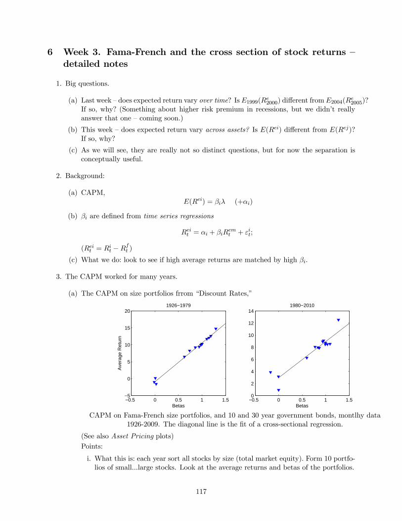
(a) The CAPM on size portfolios frrom “Discount Rates,”

−0.5 0 0.5 1 1.5−5

0

5

10

15

20

Betas

Ave

rage

Ret

urn

1926−1979

−0.5 0 0.5 1 1.50

2

4

6

8

10

12

14

Betas

1980−2010

CAPM on Fama-French size portfolios, and 10 and 30 year government bonds, montlhy data

1926-2009. The diagonal line is the fit of a cross-sectional regression.

(See also Asset Pricing plots)

Points:

i. What this is: each year sort all stocks by size (total market equity). Form 10 portfo-

lios of small...large stocks. Look at the average returns and betas of the portfolios.

117

ii. The small firm portfolio has much higher () than large firm portfolio. Thus,

yes, () does seem to vary across assets. Does this mean you should buy small

stocks? Not necessarily. The small firm beta is much larger than large firm beta!

iii. The size anomaly is the small amount by which the smallest firm portfolio lies too

far above the line. This is a glass that’s 90% full!

iv. Interestingly, the anomaly in pre 79 data disappeared when CRSP cleaned up data.

(b) Thus the “explanation” given by the CAPM,

() =

where are defined from time series regressions

= +

+ ;

( subtracts T bill rate — = − )

i. Note () = is a cross-sectional relation. The issue is , that some assets have

higher average returns than others. It’s not about “predicting” returns.

ii. Portfolios have large () because they have large . () is the thing to be

explained () is the right hand variable () and is the slope coefficient (, or

often, !)

() = +

= +

iii. are the errors — the amount by which the CAPM is wrong, the expected return

earned above and beyond compensation for risk.

iv. If () = , we say () it represents a premium for risk. Not “small stocks

are good, they pay higher ()” but “Small stocks are so risky they must pay a

high () to get people to hold them.” This is like our time-series investigation

— in bad times () is high. You might think the opposite; () high means it’s

a good time to invest. But if we all invested, we’d drive the price up and expected

return down. Differentiate when you’re asking about equilibrium vs. your own

portfolios.

v. The slope should be the mean market return. = 1 so () = 1× That’s

why we usually write

() = () +

I like to emphasize this is the slope in the graph of () vs. , but it’s the same

thing

vi. The size portfolios were a a rejection of the CAPM — the smallest firm was sta-

tistically significant. (No longer, in these data, but an open debate.)

vii. Fama and French like tables of numbers. You have to understand the idea, equation,

or plot to know what they’re talking about.

viii. Why does the CAPM “Explain?” the simplest version is, suppose a security gets

an average return twice the market, but also has a beta of two. Well, I can get

that same average return and same or less risk by just leveraging up the market (or

buying index futures, etc.)

118

ix. A bit more carefully: if you hold the market portfolio, and if a security has zero

alpha — if an expected return, higher than the market return, is matched by a beta

higher than market beta — then adding a bit of the security to your portfolio will not

improve your portfolio’s Sharpe ratio. It will be just like levering up your market

index.

4. CAPM Example 2: industry portfolios

0 0.5 1 1.50

2

4

6

8

10

12

14

NoDur

Durbl

Oil

Chems

Manuf

TelcmUtils

ShopsMoney

Other

Rf

Rm

β

E(R

e )

Time series regression (through Rm, Rf)

Cross sectional regression

Cross section, no γ

It’s not perfect, but the spread in average returns is related to betas.

(a) This is an example of how the CAPM worked ok in application after application for 20

years. It’s still a bit of a puzzle, as the SML is “too flat.” But we can make excuses for

that; betas are badly measured, etc. It doesn’t scream that the model is wrong.

(b) However, there is always a telescope, a way to make small-looking errors big (and prof-

itable.) If the “too flat SML” is real it invites “beta arbitrage:” buy low beta stocks and

short high beta stocks. Frazzini’s paper in the readings explores this fact and AQR is

trading on it.

5. The Value Puzzle

(a) FF: The CAPM works OK for size, industry, beta-sorted portfolios and many others

(all the ones anyone tried from 1970 to about 1990). What about book/market sorted

portfolios?

(b) Inspiration: like but across assets.

− ≈ +

∞X=1

−1 (∆+ − +)

Thus, if there are stocks with higher (), for whatever reason (high ), they will have

lower − . D/P reveals to us which assets (times) have high/low expected returns

by investors. FF use B/M not D/P because B is better across firms than dividends or

earnings. Many firms have = 0 0.

119

(c) Thus, we should see “low price” (High B/M) stocks have high average returns ().

It’s not surprising that “value stocks” have higher expected returns. AND we should

see them have high . Expected return alone is not a puzzle. All puzzles are joint puzzles

of expected return and beta — either high expected returns not matched by high betas, or

high/low betas not matched by expected returns.

(d) Facts: There is a big spread in average returns. But market beta is a disaster. From

“Discount rates” The () line rises as you go to value, but the × () and

×() lines do not. ( comes from a single regression, comes from the multiple

regression with FF factors too).

Growth Value −0.2

0

0.2

0.4

0.6

0.8

E(r)

β x E(rmrf)

b x E(rmrf)

h x E(hml)

Ave

rage

ret

urn

Average returns and betas

Average returns and betas for Fama - French 10 B/M sorted portfolios. Monthly data 1963-2010.

(e) Note (also in “Discount rates”) the difference pre and post 1963. Value portfolios gave

higher average returns in the earlier period, as they do now. But the CAPM worked

pretty well! The betas were right. The big puzzle post 63 is that the betas changed, not

the pattern of average returns. Again, all puzzles are joint puzzles of average returns

and betas.

120

0 0.2 0.4 0.6 0.8 10

0.2

0.4

0.6

0.8

1

G

23456

78

9

V

Rf

Betas

Ave

rage

ret

urn

1963−2009

0 0.5 1 1.50

0.2

0.4

0.6

0.8

1

1.2

Betas

1926−1963

G23

4

5 67

8 9 V

Rf

Value effect before and after 1963. Average returns on Fama - French 10 portfolios sorted by

book-to-market equity vs. CAPM betas. Monthly data. Source: Ken French’s website.

(f) Asset Pricing shows similar graphs for the 25 FF size and BM portfolios. If you want a

graphical treatment of FF’s Table 1A look there.

121

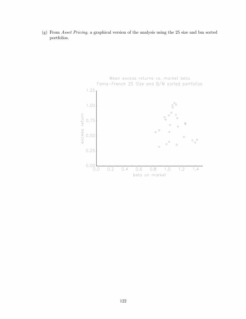
(g) From Asset Pricing, a graphical version of the analysis using the 25 size and bm sorted

portfolios.

122

123

(h) Holding size constant, B/M betas go the wrong way. Betas are lower for higher return

securities. The wrong sign is even worse than an unexplained alpha. (The Discount

Rates plot did not hold size constant, and as you can imagine

(i) To repeat, there is nothing in principle wrong with a value effect in average returns.

It’s fine if high B/M stocks have high average returns. The puzzle is: they should also

124

have high betas. The puzzle is in the betas, which go the wrong way.

6. Fama-French solution: (See Fama French Table 1)

(a) Run time series regressions that include additional factors (portfolios of stocks) SMB,

HML

= +

+ + + ; = 1 2 for each = 1 2

(b) Look across stocks at the cross-sectional implication of this time-series regression (Take

of both sides again):

() = + () + () + ()

This works pretty well ( not big) except the small growth stocks

(c) “Discount Rates” one stop summary again. Now look at the sum of red solid and red

dashed lines. () = ×() + ×().

Growth Value −0.2

0

0.2

0.4

0.6

0.8

E(r)

β x E(rmrf)

b x E(rmrf)

h x E(hml)

Ave

rage

ret

urn

Average returns and betas

Average returns and betas for Fama - French 10 B/M sorted portfolios. Monthly data 1963-2010.

125

(d) From Asset Pricing, using all 25 size and B/M portfolios. This is a graphical version of

FF’s table 1

126

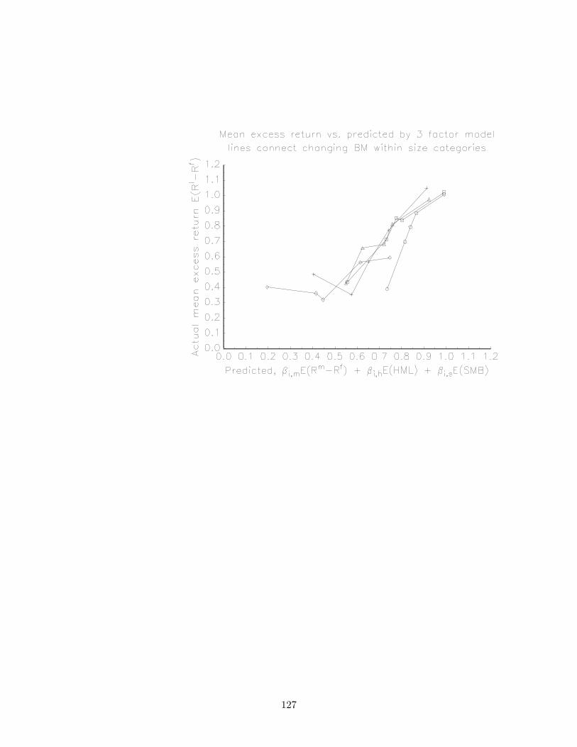
127

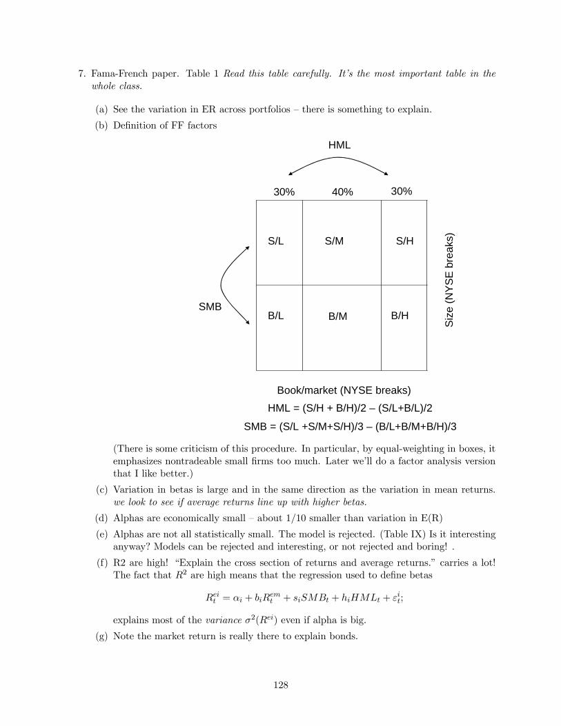
7. Fama-French paper. Table 1 Read this table carefully. It’s the most important table in the

whole class.

(a) See the variation in ER across portfolios — there is something to explain.

(b) Definition of FF factors

Book/market (NYSE breaks)

Siz

e (N

YS

E b

reak

s)

30% 30%40%

S/L S/M S/H

B/L B/M B/H

HML = (S/H + B/H)/2 – (S/L+B/L)/2

SMB = (S/L +S/M+S/H)/3 – (B/L+B/M+B/H)/3

SMB

HML

(There is some criticism of this procedure. In particular, by equal-weighting in boxes, it

emphasizes nontradeable small firms too much. Later we’ll do a factor analysis version

that I like better.)

(c) Variation in betas is large and in the same direction as the variation in mean returns.

we look to see if average returns line up with higher betas.

(d) Alphas are economically small — about 1/10 smaller than variation in E(R)

(e) Alphas are not all statistically small. The model is rejected. (Table IX) Is it interesting

anyway? Models can be rejected and interesting, or not rejected and boring! .

(f) R2 are high! “Explain the cross section of returns and average returns.” carries a lot!

The fact that 2 are high means that the regression used to define betas

= +

+ + + ;

explains most of the variance 2() even if alpha is big.

(g) Note the market return is really there to explain bonds.

128

8. Comments

(a) What’s the difference between description and explanation?What’s wrong with() =

()+()? (In fact “dissecting anomalies” does just this, but doesn’t call it

an “explanation.”) What’s wrong with “Fama and French’s model says you can explain

stock returns by size and book/market?

(b) Answer: “How you behave” not “who you are.”

i. () = () + () is a a good description. Not a good explanation.

“Fama and French’s model says you can explain stock returns by their covariance

or betas with size and book/market factors” is correct.

ii. If so, you could make money. Find small/value stocks [() () ] that have

no betas, (or form a portfolio with no beta). Make huge $ with no risk!

iii. It’s easy to change characteristic. Small companies can merge. A portfolio of small

companies is a “large” company. This does not change betas.

(c) Understand the difference between “explaining returns” (time-series regression, under-

standing the risks of investing, understanding variance and covariance) and “explaining

average returns” (cross-sectional relation between average return and beta)! Both are

interesting, but totally different concepts.

(d) Watch the language here. () = can work great — you can have a large cross-

sectional R2; you can do a good job of “explaining the cross-section of average returns”

even if the time series regression has a low 2 so you don’t “explain the cross-section of

[ex-post] returns.” And vice versa, you might have a great time-series 2 but big alphas

(intercepts in these regressions). They are different issues.

(e) Big note: The main point of FFs time series regression is not to “explain stock returns,”

a high 2. The point is to see if the are low; if high average returns are associated

with high The regressions in FF Table 1 are not by themselves the “explanation”

we’re after. They are data for that explanation — they give you the average returns and

betas. The point is to see if average returns are high where betas are high, not whether

the time-series regressions do well. This is the one most important thing to understand.

(f) Why test with portfolios and characteristics rather than just look at stocks?

i. Individual stocks have = 40− 80%, so √ makes it nearly impossible to accu-

rately measure ()Portfolios have lower by diversification, so √ is not so

bad.

ii. Betas are badly measured too, and vary over time.

iii. You need an interesting alternative. Group stocks together that might have a vio-

lation, this gives much more power.

iv. This is what people do to (try to) make money. They don’t randomly buy stocks.

They buy stocks with certain characteristics that they think will outperform. Thus,

keep tests and practice close.

v. The CAPM seemed fine (and still does) until stocks were grouped by B/M. The

CAPM still works fine for some groupings (size), not others (value) .

(g) Table 1 is a table of data for the cross-sectional relationship between () and .

We don’t really care at all about the regression in the table. Why do they show it this

way? Answer: they really want us to believe that average returns line up with betas as

they should, and see and evaluate the model’s failures.

129

9. Fama French. Is it a tautology to “explain” 25 B/M, size portfolios by 2 B/M, size portfolios?

(No)

10. → How does it work on other sorts?

(a) Sales rank is especially interesting since it is not 1/P. (quote, p. 63)

i. Note stories for betas, beyond formal tests.

ii. Sales losers behave like small value stocks.

(b) Past return sorts.

i. Focus on 12-2, 60-2, 60-13 results

ii. Note wrong sign of momentum on hml beta. Just like the discovery of HML!

iii. Note R2

(c) Jabs at Momentum:

i. High transactions costs. Will turnover all stocks at least once per year.

ii. Requires short position in small losing illiquid stocks. (November is about 1/2 of

the effect)

iii. Present in indices but not index futures.

iv. Sample sensitive. Worked less well pre 62. (But is said still to be working — all my

hedge fund buddies are still doing it).

v. Momentum is risky. In many years, last year’s winners all lose together.

vi. Very small autocorrelation 2 = 001 implies momentum (“New facts”).

vii. Will it persist? Is it a little glitch or a new parable for risk and return, leading away

from economics and to psychology?

viii. Lots of people doing it, so why does it last?

ix. But...It’s an important part of current asset allocation models

(d) Momentum factor?

i. Does it work? Yes. — If you form a portfolio of past winners, they are not guaranteed

to keep going up. (say) 55% of the time they go up, 45% of the time they go

down, so on average momentum works. But if they go down they all (tend to) go

down together. As high B/M stocks have “common movement” so past winners

move together, and a portfolio win - lose will “explain” expected returns in a factor

model.

ii. Fact:

= + + + ++

works great, “umd” factor captures 10 momentum portfolios.

iii. Does it make any sense? FF want some story about “risk premium.”

11. What is the FF model? Where does it come from?

(a) ICAPM: “State variables of concern to investors” p. 77

i. Story: People lose jobs in recessions.

ii. Gven market beta, they avoid stocks that go down in recessions→drive down prices→driveup expected returns.

130

iii. Now expected returns depend on tendency to go down in recessions as well as market

beta.

iv. HML goes down in recessions, “proxies”

(b) APT: “Minimalist interpretation.” p. 76 The central fact is high 2 in time series

regression.

i. Given hml has a premium, high time series 2 means other size and B/M portfolios

will follow. Suppose 2 = 1,

= + + + 0

→³

´= () + () + ()

ii. The same logic holds if 2 is large. Each asset is (close to) a portfolio of rmrf, hml,

smb, so must have the same return, or you can make huge profits long the asset

short the portfolio.

iii. Thus, the central puzzle is that HML seems mispriced by CAPM. Given HML

mispricing other portfolios follow by APT logic

iv. The central finding of the paper is that size, B/M portfolios move together, high 2

This survives even if the value premium disappears. “Irrational pricing” stories can

describe why mean returns of BM stocks are high, but why should they all move

together on news?

v. APT/ICAPM? Will it still work on non size-B/M portfolios? APT says only if they

still give high R2.

(c) Did you not follow that? If so, is FF really a “model”? How is this better than the

“characteristic model” () = ()? If not, Let’s spend a week thinking about

what constitutes a model!

12. Note: The conventional CAPM like the FF model is a model of variance as well as a model

for means.

= +

+

means

(

) =

2 ( ) + ( )

(Quiz: why no cross terms ()?) In matrix notation,

( 0) = 02() + Σ

Sometimes we also assume Σ is diagonal, so this is a “one factor structure.” Even if not, you

see that we are describing a lot of the covariance of returns with a single common factor.

Notice does not matter for this decomposition of variance; the relative size of 2()

and Σ, 2 and the potential diagonality of Σ do matter for “factor structure.” For our usual

quesiton about mean returns does matter (it’s everything) and 2, size or diagonality of Σ,

are basically irrelevant. (They only matter because higher 2 means higher statistics, and

thus better measures.)

13. Do we need all three factors? Why do Fama and French include smb, given that size portfolios

are perfectly explained by betas (see graph above)? This is a deep question.

131

(a) The answer is, in brief, that they could have left size out as a model of average returns,

but that size is important as a model of returns, i.e. return variance. The small stocks

often go off their own way, all together. This movement doesn’t generate an additional

premium, but it is an important component of the variance of typical (small!) stocks.

(b) For many purposes, we want to include extra factors that explain variance even if those

factors do not explain mean. For example, for risk management, you want a hedge

portfolio that closely matches the assets you’re hedging. You don’t care if there is extra

premium to the hedge portfolio, you care that its returns match your asset. Also, if we

recognize the smb factor, the residual becomes much smaller. Standard errors all depend

on the variance of the residual, so soaking up residual variance makes everything else

better measured.

(c) To see these points, go back to the CAPM. Suppose the CAPM works perfectly, and

we price an individual stock,

³

´= (

)

But suppose when we run the CAPM, we include an industry portfolio,

= +

+

+

Obviously, we will see 6= 0 — stocks load a lot on industry portfolios. If we take

averages, we see

³

´= + (

) +

³

´(28)

The industry portfolio has a positive mean (see above graph of industry portfolios).

Now, we have a puzzle. We assumed the CAPM was completely right, but it looks like

we’re going to get a multifactor model out, as both market and industry premiums are

high, and both the market and industry returns generate betas. How do we resolve this

puzzle?

(d) The easiest way to resolve this puzzle is to include an “orthogonalized” or “beta-hedged”

industry portfolio instead. (If you remember regressions, “orthogonalizing” right hand

variables is often recommended, and it makes single and multiple regression coefficients

the same.) First run

= +

+

If the CAPM is right, then

() = ()

Now construct

∗ =

−

If the CAPM is right, this beta-hedged industry portfolio has mean zero

³∗

´=

³

´− (

) = 0

Now think about running

= +

+

∗ +

What will happen?

132

i. 0, 2 improves, statistics improve, () decreases. The model of variance

improvesii.

³

´= (

) +

³∗

´= (

) + 0

The mean of the new factor is zero, so the predictions of this “two-factor model”

are the same as the predictions of the CAPM. The model of means is unchanged.

iii. Exercise: Show that the model (28) also has zero alpha and produces the same mean

return as the CAPM. Hint: Use = +

(e) As you can see, the central part of the puzzle was that and were correlated with

each other. If they had been uncorrelated to start, we wouldn’t have gotten confused.

(f) Aha. So to summarize A new factor, though useless for means, may be useful for ex-

plaining the variance of returns. The test for this situation is whether the existing factors

account for the mean of the new factor. In the case of FF, we run

= + + +

If = 0 then we can achieve the same pricing results without smb. But we will lose

2, precision, and the ability to hedge small firm return variance. If and are equal

to zero then the small stock premium () is the same as the small stock . If and are not zero and = 0, then the small stock premium exists, but it’s earned for

exposure to the other factors.

14. A summary chart of the methodology here

Group stocks by some characteristic (size, B/M, past return, etc.)

Is there a spread in average returns?

Yes

Really? Do the statistics right? Survivor/selection bias? Out of sample?

Are high average returns explained by high market betas?

Are high average returns explained by multifactor betas?

Does a new multifactor model seem plausible, work?

Trade on it. Hope it lasts.Take up behavioral financeFame and fortune

Empirical Asset Pricing Flowchart

Yes

No

Yes

No

No

Yes

No

No

Yes

133

15. A big picture for “dissecting anomalies” and the whole question of multivariate forecasts:

(a) Recall

≈

∞X=1

−1+ −

∞X=1

−1∆+

and our lovely interpretation: forecasts returns because it reveals to us market expec-

tations. If expected returns go up (some signal the market sees and we do not) then

goes down, goes up. works the same way as .

(b) Ok, but then it seems is the perfect predictor! It reveals to us everything markets

know! How can any other variables help to predict? For example, if variable says

expected returns are higher, then that means dividend yields are higher, and reveals the

information to us. We don’t need variable . Similarly, we interpreted dp forecasts to

say that 100% of variation came from expected returns. Well, if forecasts returns,

it seems like we can forecast more than 100% of returns which makes no sense!

(c) No! reveals to us the market’s expectations for the sum on the right hand side. If forecasts returns to rise and dividend growth to rise, then it can help to foreast returns

— and dividend growth. Thinking conversely, if traders’ expectations of returns and

dividend growth rose at the same time, then there would be no effect on . This is a

reasonable story for a recession — both higher growth (because the level is low) but also

higher risk aversion.

(d) Similarly, if forecasts one year returns +1 but forecasts longer term returns + to go

in the opposite direction, then it can help to forecast one year returns without affecting

(in the presence of) dp.

(e) In fact, for an extra variable to help forecast returns, it must either also forecast

dividend growth, or it must help to forecast longer term returns.

(f) Fama and French “dissecting anomalies” quotes: This is why additional “cashflow fore-

cast” anomaly variables help to forecast returns.

(g) “Discount rates” the cay experiment turns out to forecast the time path of returns.

134

1. (After reading “Dissecting anomalies”) Regressions summary. We have run a lot of different

regressions that look almost alike but are totally different in their interpretation

(a) Forecasting

+1 = + + +1; = 1 2

(b) The “market model” of returns (return variance)

= +

+ ; = 1 2 for each

(c) FF’s three-factor model of returns (return variance)

= + + + + ; = 1 2 for each

(d) The CAPM model of mean returns. (We implicitly run this when we look at expected

return vs. beta. We will run this “cross-sectional regression” explicitly soon.)

³

´= + ; = 1 2

(e) The slope coefficient in d should equal the mean market return (since its beta is one) should = (), so we sometimes force that in the implicit cross sectional “regression”

³

´= (

) + ; = 1 2

(f) Fama and French. They do option e. They are implicitly running a cross sectional

regression with the slopes equal to means of the factors. Table 1 is just data for this

regression

³

´= () + () + () + ; = 1 2

(g) The cross-sectional characteristic regression. Rather than Table 1A, FF dissecting anom-

alies and discount rates describe mean returns by a characteristic regression

³

´= + [log()] + [log()] + ; = 1 2

more generally with a vector of characteristics

³

´= + ; ; = 1 2

(h) The characteristic regression is the same thing as a forecasting regression. (Note some-

times there are fixed effects, or )

+1 = + log() + log() + ; = 1 2 = 1 2

+1 = + + +1

135

6.1 Fama and French Multifactor Anomalies Questions

NOTE: In previous years, I handed out these questions for you to mull over and then discuss in

class. This year, I took a subset and put them on the problem set for you to write out answers.

You had enough to do so I did not also post these questions. However, here they are in case you

would like a self-study guide to reading the papers. The answers follow.

Please be ready to answer, pointing to statements, numbers, or pictures in the papers. Note:

Read the bottom of p. 55 and 56. The “model” is equation (1), not equation (2)! A big point

today is to distinguish the meanings of (1) and (2)!

1. In Table 1, which kinds of stocks have higher vs. lower average returns?

2. How do Fama and French define “value” and “small” stocks?

3. Do “value” stocks have high book to market ratios or low book to market ratios?

4. Are small stocks ones with small numbers of employees, small plants, etc.

5. Do FF’s “growth” stocks have fast-growing earnings, assets, or sales?

6. Relate Fama and French’s Table 1 panel A to forecasting regressions like we ran last week?

What regression would capture the same ideas?

7. Does the spread in average returns in Table 1A present a puzzle, by itself? (Hint: why might

you not just go buy small value stocks based on the evidence of this table?)

8. How are FF’s “SMB” and “HML” factors constructed? (one sentence)

9. How is Fama and French’s Table 1 Panel B regression different from regressions you would

run to check the CAPM?

10. Can we summarize Fama and French’s model amount to saying “We can explain the average

returns of a company by looking at the company’s size and book/market ratio?”

11. Does variation in market betas across the 25 portfolios explain the variation in average returns

across the 25 portfolios?

12. What does explain variation in average returns across the 25 portfolios?

13. In “Discount rates” and overheads, I show CAPM betas explain size portfolios very well. Yet

in Table 1, market betas are about 1 across the full range of size. What explains the difference

between the results?

14. Do the strong t statistics on hml and smb in Table I, plus the large 2, verify that the Fama

French model is a good one?

15. Every model should have a test. What is the test of the FF model, and does it pass?

16. Is it a tautology to explain expected returns in 25 size and B/M portfolios by betas on size

and B/M factors?

A: No. But it’s really subtle. Consider the letter of the alphabet example.

136

17. How does a pure value sort work — not just the double sort on value and size? Does replacing

B/M with similar variables like cashflow/price or earnings/price give similar results, or is

B/M really special?

18. Which gets better returns going forward, stocks that had great past growth in sales over the

last 5 years, or stocks that had poor past growth in sales?

19. How do Fama and French explain the average returns of stocks sorted on sales growth?

20. Sales growth and B/M are very correlated across firms. In the double-sort portfolios (which

are like multiple regressions) of Table IV and V, does sales rank still help to foreast returns

controlling for B/M? Does B/M still help to forecast returns controlling for sales growth? Does

the independent movement in expected returns with sales growth, holding B/M constant,

correspond to the b, s or h betas? (Note FF don’t say much about this.)

21. Which results show the “long-term reversal” effect in average returns best? Which show the

“momentum” effect best?l pre 63.

22. Why do the sorts in Table VI stop at month -2 rather than go all the way to the minute the

portfolio is formed?

23. Does the FF model explain every anomaly thrown at it in this paper?

24. Are the returns to momentum portfolios correlated with the returns to value?

25. What is FF’s “minimalist” interpretation of their model (p. 5, p. 75)

26. Do FF think their model is a ICAPM or an APT? What do you think?

27. It looks like we should all buy value, but we can’t all buy value, someone has to hold the

growth stocks. If we all try to buy value, the value effect will disappear because we drive

up the prices. How to Fama and French address this conundrum? Do they think investors

are just too behavioral to notice value? Do they think the effect will go away when investors

wake up? (hint, p. 76, 77)

28. Momentum seems to be a big problem for the model. What do Fama and French have to say

about momentum?

29. (Though about the introduction, these are easier to answer after you’ve read the paper.) On

p. 55, why do FF refer to (1) as their “model,” and not (2)?

30. On p. 56, FF say ”the three factor model in (1) seems to capture much of the cross-sectional

variation in average stock returns” (my emphasis). What result in what table supports this

statment?

31. on p. 56, bottom, FF say “the three factor model in (1) and (2)...is a parsimonious description

of returns and average returns.” Why did they add (2) and make the distinction between

“returns” and “average returns?” What additional results in what table support the “returns”

word?

137

6.2 Discount rates questions

These questions cover only this week’s reading, p. 1058-1064.

1. Figure 6 says expected returns are higher for value portfolios. Does the paper say this is the

value puzzle?

2. What central feature of Figure 6 captures FF’s “explanation” of the value puzzle?

3. On p. 1060 I say ”Covariance is in a sense Fama and French’s central result.” What table or

set of numbers in Fama and French convey this result?

4. What regression does “discount rates” suggest to provide the same information as FF’s Table

1A, in the same way we forecast returns last week?

6.3 Fama and French Dissecting Anomalies Questions

The point of this paper is to look at momentum, and a bunch of additional variables that appeared

since the size and B/M work. Are they real? Are they subsumed in size, B/M? Are they all

independent, or are some subsumed by others? (1654 “which have information about average returns

that is missed by the others.”) The paper also looks at what anomalies are there in big stocks, vs.

what is just a feature of microcaps, which can’t really be exploited. Take some time with this paper

to really digest Table 2 and 4. Finally, the paper agonizes about functional form. Is expected

return really related to a firm’s B/M, to the log of B/M, to which decile of B/M a firm is in,

etc.? Note the entire object of the paper is to extend Table 1 panel A of multifactor anomalies,

the description of expected returns as a function of characteristics. Many of the variables have

inspiration as cashflow forecasts — variables which forecast cash flows should help B/M to forecast

returns. My questions go through the tables and facts first, then come back to the introduction

1. How do FF define “Microcap” and “small” stocks? What percentage of stocks are “Micro”?

What fraction of market value do “micro” stocks comprise? How can the percentile break-

point that defines tiny be different from the fraction of tiny stocks in the sample?

2. Do small and micro stocks have different mean and standard deviation of returns than bigger

stocks? Why are the VW and EW average returns in Table I so different?

3. Are the average returns in Table II raw, excess, or adjusted somehow? Do they represent

returns, or alphas, or something else?

4. Explain the first row of Momentum and then Net stock issues (Market) in Table II. What do

the numbers mean?

5. Why are the t- statistics for the High-Low portfolio so much better than for the individual

portfolios?

6. Which anomalies produce strong average hedge returns for all three size groups? What num-

bers in Table II document your answer? (Hint: start by reading the H-L returns, then the

H-L t stats, then look at the remaining columns)

7. Which anomalies seem only to work in tiny stocks in Table II?

138

8. Which anomaly gives the highest Sharpe ratio in Table II? (Help, there are no Sharpe ratios

in Table II! Hint: how is a t statistic computed? You can translate from t to Sharpe ratios.)

9. The Profitability sort seems not to work in Table II. (Point to numbers). How did people

think it was there? (Hint: 1663 pp2) ns, not each variable at a time.

10. Explain why the numbers in Table III jump so much between 4 and high.

Note on the way to Table IV. Table IV has “Fama-MacBeth regressions”. We’ll study those

in detail a bit later. For now, you can think of them as regressions across individual stocks i,

to determine how average returns depend on characteristics like size and book/market,

³´= + 1 log() + 2 log() + 3 + + ; = 1 2

If all works well, this regression gives the same information as splitting things into 5 groups

and looking at group means. But the paper is all about the pitfalls of each method vs. the

other. One reason for doing regressions is there is no way to split things into groups based

on 2,3,4, etc. variables, to see whether, for example, momentum is still important after ac-

counting for size and B/M. 1666 below III, “which anomalies are distinct and which have

little marginal ability to predict returns?” But regressions need to take more of a stand on

functional form, which FF worry about a lot. (“pervasive” is also about functional form

though. It’s only “pervasive” if expected returns are linear in the portfolio number.)

Log(Book/market)

E(R)

1 2 3 4 5Portfolio

PortfolioMean

Securities

Better weights?

Sorted portfolios and cross-sectional regressions.

139

Log(Book/market)

E(R)

A warning on OLS equally-weighted cross-sectional regressions

11. Explain what the first two rows of MC and B/M columns mean in Table IV.

12. “The novel evidence is that the market cap (MC) result draws[size effect] much of its power

from microcaps.” (p. 1667) What numbers in Table IV are behind this conclusion?

13. Should the intercept be zero in the regressions of Table IV?

14. What is a “good” pattern of results in Table IV? Which variables have it, and which do not?

15. Overall, do any of the anomaly variables drive the other ones out in a multiple regression

sense, or does each seem to give a separate piece of information about expected returns?

16. In the conclusions p. 1675, FF say “The evidence..is consistent with the standard valuation

equation which says that controlling for B/M, higher expected net cashflows...imply higher

expected stock returns” and “Holding the current book-to-market ratio fixed, firms with

high expected future cash flows must have high expected returns” Isn’t this the fallacy that

“profitable companies have higher stock returns” , or “confusing good companies with good

stocks”? (Hint: “controlling for B/M” is important! Think about our present value identity.)

17. FF start out comparing regressions and sorts (1654, top). How is a regression the same thing

as a sort? What regression would you run to achieve the same thing as a BM sort?

18. FF point out dangers of the common practice of sorting stocks by some variable, and then

looking at the average returns of the 1-10 spread portfolio. What don’t they like about this

practice?

19. FF continue by pointing out advantages and disadvantages of cross sectional regressions vs.

portfolio sorts. What are they?

Note: If you can’t directly answer the following questions from the paper, at least think

about what else you need to know in order to figure out the answer.

20. Do these new average returns correspond to new dimensions of common movement across

stocks, as B/M and size corresponded to B/M and size factors?

140

21. What is the highest Sharpe ratio you can get from exploiting one of these anomalies? (Choose

any one).

22. What is the highest Sharpe ratio you can get from combining all these anomalies and exploit-

ing them as much as possible?

23. It seems we get better returns and higher t statistics the finer we chop portfolios. Can you

make anything look good by making 100 portfolios and then looking at the 1-100 spread? (FF

don’t talk about this, it’s a puzzle for you. An accurate answer takes a few equations, but

just think through the issue and guess what would happen as you subdivide finer and finer.)

6.4 Discount rates multivariate sections questions

These questions cover p. 1053-1058 and 1058-1064, and 1098-1099

1. Dooes cay help to forecast market returns?

2. In the context of the present value identity, how can cay help to forecast returns given that

dividend yields reveal the market’s return foreast?

3. In what way do the first two columns of Figure 5 differ from the impulse-response function

based only on returns and dp that you calculated?

4. In the final column of Figure 5, which components of the present value identity also change

so that cay can help to forecast one-year returns without changing the dividend yield

5. On the top of p. 1062 I advocate running some regressions. Which Fama French table runs

regressions like these?

6. How does the “cross-secton” log(B/M) coefficient in Table AIII compare to the coefficients

in FF’s Table IV? (Roughly). Why is the “portfolio dummies” coefficient so much larger?

141

6.5 Fama and French Multifactor Anomalies Questions and Answers

Note: Read the bottom of p. 55 and 56. The “model” is equation (1), not equation (2)! A big

point today is to distinguish the meanings of (1) and (2)!

1. In Table 1, which kinds of stocks have higher vs. lower average returns?

A: Value and small. Table 1 panel A

2. How do Fama and French define “value” and “small” stocks?

A: Table I caption. Based on total market value of equity, and ratio of market value to book

value. They form portfolios every year based on June values.

3. Do “value” stocks have high book to market ratios or low book to market ratios?

A: Remember low market value, hence high B/M.

4. Are small stocks ones with small numbers of employees, small plants, etc.

A: Not necessarily. It’s a market value sort, not a book value or other sort. Thus, it’s also

a 1/price kind of variable. In fact, it turns out that “small” companies, with small numbers

of employees, book assets, etc., don’t earn any special returns. The returns are good only if

you define “small” in a way that involves low market prices.

5. Do FF’s “growth” stocks have fast-growing earnings, assets, or sales?

A: No and this is important. Wall street “growth” stocks means stocks with fast-growing

earnings or similar features. FF mean just “high market/book” stocks, i.e. “overpriced”

stocks. Getting definitions straight is 90% of the battle in this business. It turns out that

FF’s “‘growth” stocks usually are growing fast, high turnover, etc., but that’s not how FF

define them. (That’s documented in other FF papers. Here, note that high sales-growth

companies have “growth” values of . ) Wall St. terminology is different, however, and

worth remembering. “Growth” managers would be insulted if you told them they invest in

overpriced stocks!

6. Relate Fama and French’s Table 1 panel A to forecasting regressions like we ran last week?

What regression would capture the same ideas?

A: They don’t run regressions in this paper (Yes in other papers). They just form portfolios

based on B/M and size in year t and see how they do in year t+1. It’s basically the same thing

of course. Table 1 Panel A is basically this, with = average return and = book/market

ratio. So they could have run +1 = + () + +1. “Discount rates” talks a lot

about this equivalence.

142

x

y

7. Does the spread in average returns in Table 1A present a puzzle, by itself? (Hint: why might

you not just go buy small value stocks based on the evidence of this table?)

A: It would not be a puzzle if betas where high where expected returns are high. Then the

high returns would be compensation for risk.

8. How are FF’s “SMB” and “HML” factors constructed? (one sentence)

A: See Table 1 caption. Basically as big portfolios of large - small and value - growth firms.

There is some criticism of FF that the HML factor equally weights the subcategories, giving

it a bias towards small firms.

9. How is Fama and French’s Table 1 Panel B regression different from regressions you would

run to check the CAPM?

A: It’s the same, but there are more factors on the right hand side.

10. Can we summarize Fama and French’s model amount to saying “We can explain the average

returns of a company by looking at the company’s size and book/market ratio?”

A: NO. The model says you get high average returns for covarying with the B/M portfolio,

not for being a high B/M firm. A firm that was value but acted like growth should get the

growth premium.

11. Does variation in market betas across the 25 portfolios explain the variation in average returns

across the 25 portfolios?

A: No, market betas are all about one. Table 1, Panel B

12. What does explain variation in average returns across the 25 portfolios?

A: size (s) and book/market (b) betas. Table 1 Panel B

13. In “Discount rates” and overheads, I show CAPM betas explain size portfolios very well. Yet

in Table 1, market betas are about 1 across the full range of size. What explains the difference

between the results?

A: Multiple regression vs. single regression. The CAPM explains SMB pretty well too. But

size correlates with SMB, so in a multiple regression we see SMB betas take over from CAPM

143

betas. This does not mean the CAPM is wrong — the capm says that average returns line

up with single regression betas on the market, not with multiple regression betas. This table

does not show the CAPM is wrong — you need another table for that that uses only single

regression betas. As an example, industry portfolios will always enter if you add them, even

if the CAPM is right.

14. Do the strong t statistics on hml and smb in Table I, plus the large 2, verify that the Fama

French model is a good one?

A: NO. or at least not for this purpose. The model is (1) not (2), the purpose is to understand

average returns, not the variation in returns, the question is whether intercepts (alphas) are

zero. Strong betas and high 2 are meaningful, to say the model captures a lot of risk, it

is a good description of returns (i.e. variation in returns), but not that it captures average

returns.

15. What meaning does the 2 in Table I have? What words from the paper follow from the 2

values

A:The 2 is important. Where there is mean there must be covariation, otherwise Sharpe

ratios would explode. It reflects the fact that all the value stocks move up and down together.

They must do this, so that the diversified portfolio of HML only earns its premium and not

an astronomical Sharpe ratio. This is the “APT’ interpretation of Fama and French. As we

will see the “APT” states that a high 2 implies that alphas can’t be too big. Words like

“explains returns” as opposed to “explains average returns” refer to the 2.

16. Every model should have a test. What is the test of the FF model, and does it pass?

Answer: the test is whether the alphas are jointly equal to zero. P. 57, “The F test... ” reports

that it fails. The reason though is that the 2 are so high. It’s like a t test — () can

be large because () is low, not because is large. The model’s success is that the alphas

are so small. Statistics lets us show that the glass is only 95% full, and the 5% is not due

to chance. The point of looking at all the tables is that the glass is indeed 95% full! It’s an

interesting comment on statistics that this, the most successful model in the last 20 years, is

decisively rejected.

17. Is it a tautology to explain expected returns in 25 size and B/M portfolios by betas on size

and B/M factors?

A: No. But it’s really subtle. Consider the letter of the alphabet example.

18. How does a pure value sort work — not just the double sort on value and size? Does replacing

B/M with similar variables like cashflow/price or earnings/price give similar results, or is

B/M really special?

A: Table II/III top

19. Which gets better returns going forward, stocks that had great past growth in sales over the

last 5 years, or stocks that had poor past growth in sales?

A: Poor — see Table II.

20. How do Fama and French explain the average returns of stocks sorted on sales growth?

A: Table III it’s mostly a value effect. I love this one because it has no price in it at all.

And Wall Street intuition goes exactly the other way. Again, the expected returns “should”

correspond to beta — low sales firms should have higher average returns — and higher betas!

144

21. Sales growth and B/M are very correlated across firms. In the double-sort portfolios (which

are like multiple regressions) of Table IV and V, does sales rank still help to foreast returns

controlling for B/M? Does B/M still help to forecast returns controlling for sales growth? Does

the independent movement in expected returns with sales growth, holding B/M constant,

correspond to the b, s or h betas? (Note FF don’t say much about this.)

A: I put the numbers in a table to get a better sense, as I couldn’t follow the 1-2 stuff.

Holding sales growth constant, you still see very strong value effects. Holding B/M constant,

however, I see almost negligible sales growth effects. 0.47 to 0.52, 0.93 to 1.11. And since

these are big portfolios, the low sales growth might be tilted to more value firms within the

portfolios.Average returns (Table IV)

sales

high med low

growth 0.47 0.49 0.52

B/M 0.64 0.69 0.74

value 0.93 0.94 1.11

The market bs are all 1 as usual.

market betas b (Table V)

sales

high med low

growth 1.10 1.03 1.00

B/M 1.12 1.00 0.99

value 1.17 1.06 1.01

The small s’s increase as you go down. Value firms are also small. As we move right to left,

we see the usual U shaped pattern — extremes are more volatile firms, and small firms are

more volatilesml betas s

sales

high med low

growth 0.49 0.31 0.55

B/M 0.63 0.48 0.50

value 0.87 0.74 0.97

Now, the interesting part. The hml betas increase as you go down, as they should. The hml

betas do not increase as you go from left to right, though the expected returns did. Both are

slight, so it’s not really a rejection of the model. Both might really be flat as you go from

left to right. So I really read it that sales growth worked only as a proxy for B/M. However,

the point estimates say that the slight rise in expected returns as you go from left to right is

contradicted by the slight decline of h as you go from left to right.

hml betas h

sales

high med low

growth -0.33 -0.14 -0.04

B/M 0.31 0.25 0.32

value 0.75 0.70 0.68

145

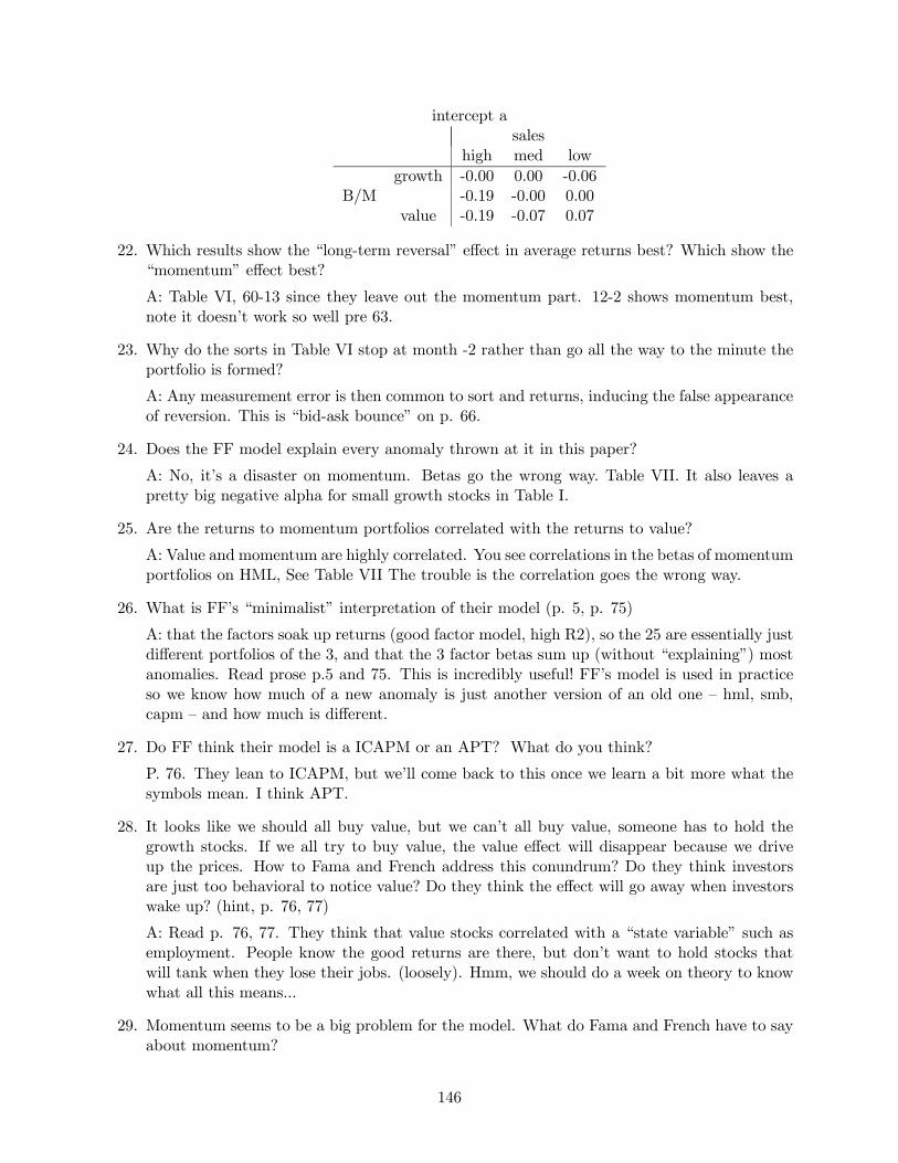
intercept a

sales

high med low

growth -0.00 0.00 -0.06

B/M -0.19 -0.00 0.00

value -0.19 -0.07 0.07

22. Which results show the “long-term reversal” effect in average returns best? Which show the

“momentum” effect best?

A: Table VI, 60-13 since they leave out the momentum part. 12-2 shows momentum best,

note it doesn’t work so well pre 63.

23. Why do the sorts in Table VI stop at month -2 rather than go all the way to the minute the

portfolio is formed?

A: Any measurement error is then common to sort and returns, inducing the false appearance

of reversion. This is “bid-ask bounce” on p. 66.

24. Does the FF model explain every anomaly thrown at it in this paper?

A: No, it’s a disaster on momentum. Betas go the wrong way. Table VII. It also leaves a

pretty big negative alpha for small growth stocks in Table I.

25. Are the returns to momentum portfolios correlated with the returns to value?

A: Value and momentum are highly correlated. You see correlations in the betas of momentum

portfolios on HML, See Table VII The trouble is the correlation goes the wrong way.

26. What is FF’s “minimalist” interpretation of their model (p. 5, p. 75)

A: that the factors soak up returns (good factor model, high R2), so the 25 are essentially just

different portfolios of the 3, and that the 3 factor betas sum up (without “explaining”) most

anomalies. Read prose p.5 and 75. This is incredibly useful! FF’s model is used in practice

so we know how much of a new anomaly is just another version of an old one — hml, smb,

capm — and how much is different.

27. Do FF think their model is a ICAPM or an APT? What do you think?

P. 76. They lean to ICAPM, but we’ll come back to this once we learn a bit more what the

symbols mean. I think APT.

28. It looks like we should all buy value, but we can’t all buy value, someone has to hold the

growth stocks. If we all try to buy value, the value effect will disappear because we drive

up the prices. How to Fama and French address this conundrum? Do they think investors

are just too behavioral to notice value? Do they think the effect will go away when investors

wake up? (hint, p. 76, 77)

A: Read p. 76, 77. They think that value stocks correlated with a “state variable” such as

employment. People know the good returns are there, but don’t want to hold stocks that

will tank when they lose their jobs. (loosely). Hmm, we should do a week on theory to know

what all this means...

29. Momentum seems to be a big problem for the model. What do Fama and French have to say

about momentum?

146

A: p. 81. Maybe it’s data snooping and will go away. (It didn’t) Maybe it’s irrational,

but they caught the behavioral guys making up new theories for every fact. Maybe we need

another factor. (let’s hope not!) Alas, it does seem to be another factor; it’s much harder

to come up with any ”rational” or ”irrational” story for it. Rational — why should we care

about these stocks? Irrational — why should they all move together ex post? Note it’s hard

to trade, and requires turning over the portfolio every year. It also is a “new telescope” for

small autocorrelation, and a tiny component of asset prices (”discount rates”) because it lasts

so short a time.

30. (Though about the introduction, these are easier to answer after you’ve read the paper.) On

p. 55, why do FF refer to (1) as their ”model,” and not (2)?

A: The point of the model is expected returns. (2) only defines the betas. Taking the mean

of (2), you get an term in (1). The point of (1) is that it has no term.

31. On p. 56, FF say ”the three factor model in (1) seems to capture much of the cross-sectional

variation in average stock returns” (my emphasis). What result in what table supports this

statment?

A: 2 in Table I

32. on p. 56, bottom, FF say “the three factor model in (1) and (2)...is a parsimonious description

of returns and average returns.” Why did they add (2) and make the distinction between

“returns” and “average returns?” What additional results in what table support the “returns”

word?

A: (2) is a description of variance, and the high 2 makes it a good “description of returns.”

(1) is a description of mean returns, and the low or zero means mean returns are high

where betas are high.

6.6 Discount rates questions and answers

These questions only reflect the cross sectional section p. 1058-1064.

1. Figure 6 says expected returns are higher for value portfolios. Does the paper say this is the

value puzzle?

A: No. The puzzle is that betas don’t also rise, p. 1058 ”The fact that betas do not rise with

value is really the heart of the puzzle”

2. What central feature of Figure 6 captures FF’s “explanation” of the value puzzle?

A: The fact that ×() lines up with (). “Higher average returns do line up well with

larger values of the regression coefficient.” 1059

3. On p. 1060 I say ”Covariance is in a sense Fama and French’s central result.” What table or

set of numbers in Fama and French convey this result?

A: The large 2 in Table 1 B

4. What regression does “discount rates” suggest to provide the same information as FF’s Table

1A, in the same way we forecast returns last week?

A: +1 = + × + × + +1, top of p. 1062 ( includes BEME and ME)

147

6.7 Fama and French Dissecting Anomalies Q and A

The point of this paper is to look at momentum, and a bunch of additional variables that appeared

since the size and B/M work. Are they real? Are they subsumed in size, B/M? Are they all

independent, or are some subsumed by others? (1654 “which have information about average returns

that is missed by the others.”) The paper also looks at what anomalies are there in big stocks, vs.

what is just a feature of microcaps, which can’t really be exploited. Take some time with this paper

to really digest Table 2 and 4. Finally, the paper agonizes about functional form. Is expected

return really related to a firm’s B/M, to the log of B/M, to which decile of B/M a firm is in,

etc.? Note the entire object of the paper is to extend Table 1 panel A of multifactor anomalies,

the description of expected returns as a function of characteristics. Many of the variables have

inspiration as cashflow forecasts — variables which forecast cash flows should help B/M to forecast

returns. My questions go through the tables and facts first, then come back to the introduction

1. How do FF define “Microcap” and “small” stocks? What percentage of stocks are “Micro”?

What fraction of market value do “micro” stocks comprise? How can the percentile break-

point that defines tiny be different from the fraction of tiny stocks in the sample?

A: 1656 or Table 1. The breakpoints are the 20% and 50% percentiles of the NYSE. 60% of

stocks are micro, but account for 3% of microcaps. Most stocks are tiny. Most value is in a

few large stocks. This means that equally weighted portfolios will always be weighted towards

really small stocks. The sample includes amex and nasdaq which have many smaller stocks

than NYSE, and breakpoints come from NYSE

2. Do small and micro stocks have different mean and standard deviation of returns than bigger

stocks? Why are the VW and EW average returns in Table I so different?

A: Larger mean, and a good deal larger volatility.

3. Are the average returns in Table II raw, excess, or adjusted somehow? Do they represent

returns, or alphas, or something else?

A: They are “characteristic-adjusted”, explained 1658 below II. sorts. This means, find the

portfolio of 25 size/book/market whose size and B/M are closest, and subtract off that return.

The text says that true size and book/market alphas gives similar results, though since there

are some big alphas (small/growth) separating average returns and betas in the 25, I’m not

altogether convinced. OTOH, FF argue that individual-stock hml, smb betas are measured

badly and wander over time. Thus, they say, the characteristic is a better measure of beta

than beta itself. Anyway, read the table as FF’s ideas about alphas after controlling for size

and b/m.

4. Explain the first row of Momentum and then Net stock issues (Market) in Table II. What do

the numbers mean?

A: this just leads to a discussion to make sure we understand table construction.

5. Why are the t- statistics for the High-Low portfolio so much better than for the individual

portfolios?

A: We’re really not that interested in whether portfolio excess returns are different from zero.

We want to know if they’re different from each other. If all averages were equal to each

other but different from zero, it wouldn’t be that interesting. Each portfolio could be within

148

a standard error of zero, but if the long-short portfolio is significant, you have a trading

strategy/anomaly.

6. Which anomalies produce strong average hedge returns for all three size groups? What num-

bers in Table II document your answer? (Hint: start by reading the H-L returns, then the

H-L t stats, then look at the remaining columns)

A: read 1662 pp3. Issues, accruals, and momentum. Look at the High-Low number. Look

for consistency across 4 size groupings, and consistency across VW and EW results.

Note: FF are really interested in what goes on in the microcap range. I’ll focus on the results

that survive in the big ranges.

7. Which anomalies seem only to work in tiny stocks in Table II?

A: Asset growth. Look at the numbers.

8. Which anomaly gives the highest Sharpe ratio in Table II? (Help, there are no Sharpe ratios

in Table II! Hint: how is a t statistic computed? You can translate from t to Sharpe ratios.)

A: = ()³()

ë;()() =

√ To annualize()() =

√12 ×

√ =

p,

p =

√425 = 6 52 Thus, a = 326 translates to the market

Sharpe ratio 0.5, and a t=6.52 translates to a Sharpe ratio of 1. Hedge funds think they can

find Sharpes of 2 or more — good luck. Most of the ts are between 3 and 5, especially if you

only look at big firms.

9. The Profitability sort seems not to work in Table II. (Point to numbers). How did people

think it was there? (Hint: 1663 pp2)

A: 1663 pp2 With controls for cap and B/M. There is a profitability effect on its own, but

size and B/M pick it up. This is a good instance of the point of the paper — what works in

the presence of the others, what has marginal power, what is the multiple regression forecast

of returns, not each variable at a time.

10. Explain why the numbers in Table III jump so much between 4 and high.

A: The 1/5 of extreme values of any distribution is way spread out. Table III momentum

lets you make the connection between autocorrelation and momentum. Compare the mean

returns and the spread in right hand variable between II and III. This is a case in which

momentum itself rather than the portfolio number (which squishes the tails) might be a

better variable. Functional form! Other cases work differently. Make a graph showing how

distributions lead to large values of the x variable for the tails. Compare the returns in III

to the average returns in II to infer the autocorrelation coefficient behind momentum.

Note on the way to Table IV. Table IV has “Fama-MacBeth regressions”. We’ll study those

in detail a bit later. For now, you can think of them as regressions across individual stocks i,

to determine how average returns depend on characteristics like size and book/market,

³´= + 1 log() + 2 log() + 3 + + ; = 1 2

If all works well, this regression gives the same information as splitting things into 5 groups

and looking at group means. But the paper is all about the pitfalls of each method vs. the

other. One reason for doing regressions is there is no way to split things into groups based

149

on 2,3,4, etc. variables, to see whether, for example, momentum is still important after ac-

counting for size and B/M. 1666 below III, “which anomalies are distinct and which have

little marginal ability to predict returns?” But regressions need to take more of a stand on

functional form, which FF worry about a lot. (“pervasive” is also about functional form

though. It’s only “pervasive” if expected returns are linear in the portfolio number.)

Log(Book/market)

E(R)

1 2 3 4 5Portfolio

PortfolioMean

Securities

Better weights?

Sorted portfolios and cross-sectional regressions.

Log(Book/market)

E(R)

A warning on OLS equally-weighted cross-sectional regressions

11. Explain what the first two rows of MC and B/M columns mean in Table IV.

A: you’re seeing the basic size and B/M effects in expected returns. Larger size means smaller

ER, Larger B/M means larger ER. (see bottom 1667.)

12. “The novel evidence is that the market cap (MC) result draws[size effect] much of its power

from microcaps.” (p. 1667) What numbers in Table IV are behind this conclusion?

A: This is the disappearance of the size coefficient in the other groups in the top left part of

Table IV. Note size is also much weaker post 1979 — when the size effect was published and

small stock funds started. (not in this paper)

150

13. Should the intercept be zero in the regressions of Table IV?

A: NO. These are “description” regressions, () = + ln + ln() + They

correspond to Table 1A of FF 1996. These are not “explanation” regressions the right hand

variables are not betas.

14. What is a “good” pattern of results in Table IV? Which variables have it, and which do not?

A: we’re looking for a large coefficient and t stat, and we want the coefficient to be consistent

in the size groupings. Nonzero Issues and momentum are the only ones that do (1669)

15. Overall, do any of the anomaly variables drive the other ones out in a multiple regression

sense, or does each seem to give a separate piece of information about expected returns?

A: Table IV the ones that were individually significant all seem to survive, Except Zero NS.

16. In the conclusions p. 1675, FF say “The evidence..is consistent with the standard valuation

equation which says that controlling for B/M, higher expected net cashflows...imply higher

expected stock returns” and “Holding the current book-to-market ratio fixed, firms with

high expected future cash flows must have high expected returns” Isn’t this the fallacy that

“profitable companies have higher stock returns” , or “confusing good companies with good

stocks”? (Hint: “controlling for B/M” is important! Think about our present value identity.)

A: Note the crucial “holding B/M fixed.” Holding price fixed, anything that forecasts cashflows

must also forecast returns. Go back to our linearized present value formula,

− =

∞X=1

−1∆+ −

∞X=1

−1+

The fallacy is that high ∆+ means nothing about , because it just means high − . But

holding p-d constant high∆must also come with high . In that sense, the cashflow variables

can be thought of as “cleaning up” B/M for the fact that B/M forecasts both cashflows and

returns.

Now, having seen what’s in the paper, let’s go back and read the introduction:

17. FF start out comparing regressions and sorts (1654, top). How is a regression the same thing

as a sort? What regression would you run to achieve the same thing as a BM sort?

A: +1 = + () + +1 means that if you sort stocks by higher BM, those will have

× higher returns.

18. FF point out dangers of the common practice of sorting stocks by some variable, and then

looking at the average returns of the 1-10 spread portfolio. What don’t they like about this

practice?

A: 1654. Their main complaint is that these portfolios are equal-weighted, thus focusing on

tiny stocks.

19. FF continue by pointing out advantages and disadvantages of cross sectional regressions vs.

portfolio sorts. What are they?

A: 1654 bottom. Functional form, microcaps can dominate because more of them and wider

spreads in anomalies (draw a picture). Statistician: We can fix that, it’s called GLS.

Note: If you can’t directly answer the following questions from the paper, at least think

about what else you need to know in order to figure out the answer.

151

20. Do these new average returns correspond to new dimensions of common movement across

stocks, as B/M and size corresponded to B/M and size factors?

A: This paper does not go on to do the next obvious question: do we now have 5 or 6 factors?

21. What is the highest Sharpe ratio you can get from exploiting one of these anomalies? (Choose

any one).

A: That also depends on the covariance structure. If the stocks or portfolios sorted on a

new anomaly are independent, Sharpe ratios go through the roof. If there are also common

factors, the sharpe ratios from diversified portfolios that load on new anomalies is not so

large. We know the individual portfolio sharpe ratios are 0.5-1.0 from the t stats, though,

and we know these are uncorrelated from the market, so we know there are some interesting

Sharpe ratios in here, even if there are new common factors!

22. What is the highest Sharpe ratio you can get from combining all these anomalies and exploit-

ing them as much as possible?

A: Again, we don’t know without knowing a) are there new common factors b) how correlated

are the new common factors. Next paper please!

23. It seems we get better returns and higher t statistics the finer we chop portfolios. Can you

make anything look good by making 100 portfolios and then looking at the 1-100 spread? (FF

don’t talk about this, it’s a puzzle for you. An accurate answer takes a few equations, but

just think through the issue and guess what would happen as you subdivide finer and finer.)

A: No. First, you’re sorting on microcaps which you may not trust. More importantly, the

variance goes up as well, so the sharpe ratio and the t statistic ³√´should stabilize

as you get more extreme. Discount rates p. 1029 has a calculation.

6.8 Discount rates multivariate questions and answers

These questions cover p. 1053-1058 and 1058-1064, and 1098-1099. See also Week 1 notes on the

impulse response function with cay

1. Dooes cay help to forecast market returns?

A: That’s a bit of a trick question. It helps to foreacast one year returns a lot, with t = 3.19.

But it does not help to forecast long run returns at all.

2. In the context of the present value identity, how can cay help to forecast returns given that

dividend yields reveal the market’s return foreast?

A: If cay forecasts +1 then it must either also forcast longer horizon returns, or it must

forecast dividend growth, because dp gives the sum of long-run return and dividend growth

forecasts. (Bottom of 1054)

3. In what way do the first two columns of Figure 5 differ from the impulse-response function

based only on returns and dp that you calculated?

A: It doesn’t, it’s pretty much the same

4. In the final column of Figure 5, which components of the present value identity also change

so that cay can help to forecast one-year returns without changing the dividend yield

152

A: It’s mostly long-run returns. There isn’t that much effect on long-run dividend growth.

(Text, bottom of 1057)

5. On the top of p. 1062 I advocate running some regressions. Which Fama French table runs

regressions like these?

A: Dissecting anomalies, Fama MacBeth regressions Table IV

6. How does the “cross-secton” log(B/M) coefficient in Table AIII compare to the coefficients

in FF’s Table IV? (Roughly). Why is the “portfolio dummies” coefficient so much larger?

A: They’re about the same, -0.27 and -0.28. p. 1099, “Variation over time in a given portfolio’s

book-to-market ratio is a much stronger signal of return variation than the same variation

across portfolios in average book-to-market ratio.”

153