6. Representing Rotation - Computer Sciencetrink/Courses/RobotManipulation/lectures/lecture6.pdf · Lecture 6. Representing Rotation. Chapter 1 Manipulation 1 ... 6.4 Graphical representation

6. Representing RotationMechanics of Manipulation

Matt [email protected]

http://www.cs.cmu.edu/~mason

Carnegie Mellon

Lecture 6. Mechanics of Manipulation – p.1

Lecture 6. Representing Rotation.

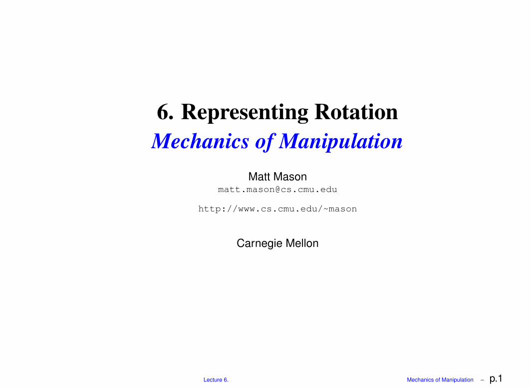
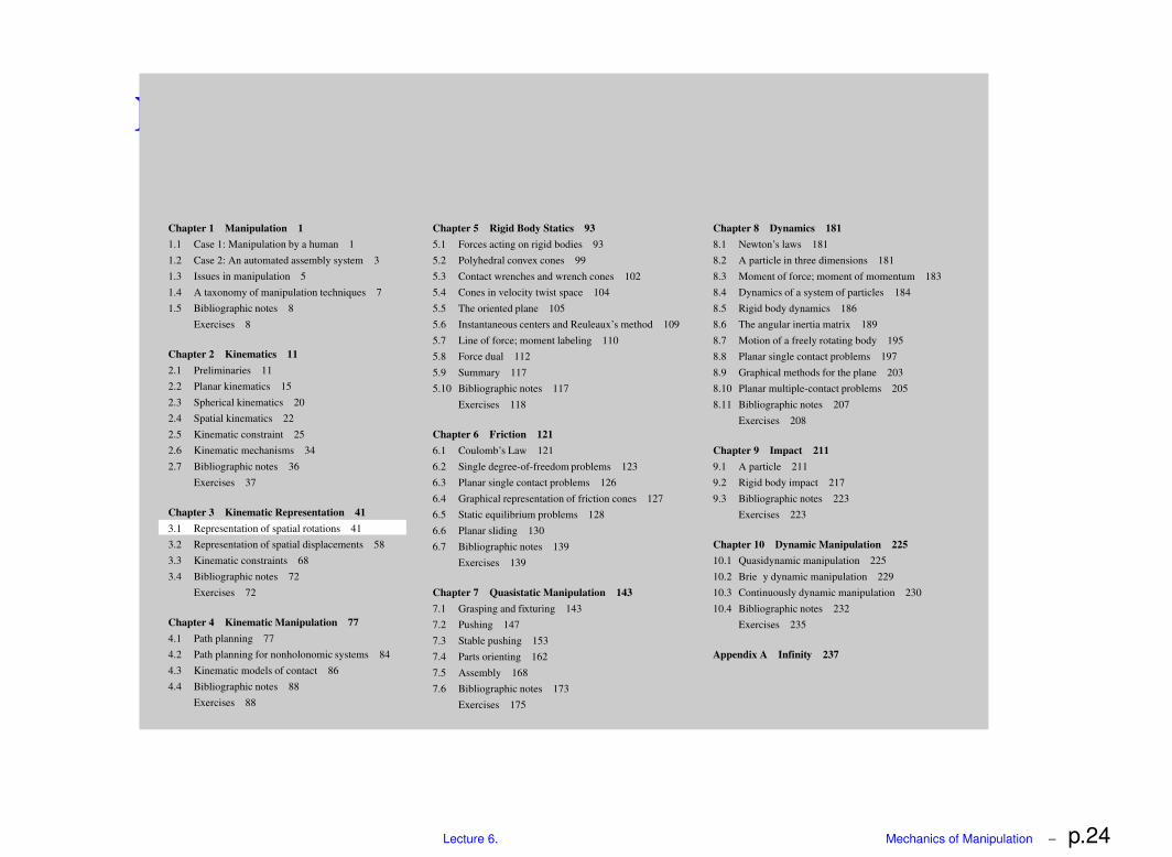
Chapter 1 Manipulation 11.1 Case 1: Manipulation by a human 11.2 Case 2: An automated assembly system 31.3 Issues in manipulation 51.4 A taxonomy of manipulation techniques 71.5 Bibliographic notes 8

Exercises 8

Chapter 2 Kinematics 112.1 Preliminaries 112.2 Planar kinematics 152.3 Spherical kinematics 202.4 Spatial kinematics 222.5 Kinematic constraint 252.6 Kinematic mechanisms 342.7 Bibliographic notes 36

Exercises 37

Chapter 3 Kinematic Representation 413.1 Representation of spatial rotations 413.2 Representation of spatial displacements 583.3 Kinematic constraints 683.4 Bibliographic notes 72

Exercises 72

Chapter 4 Kinematic Manipulation 774.1 Path planning 774.2 Path planning for nonholonomic systems 844.3 Kinematic models of contact 864.4 Bibliographic notes 88

Exercises 88

Chapter 5 Rigid Body Statics 935.1 Forces acting on rigid bodies 935.2 Polyhedral convex cones 995.3 Contact wrenches and wrench cones 1025.4 Cones in velocity twist space 1045.5 The oriented plane 1055.6 Instantaneous centers and Reuleaux’s method 1095.7 Line of force; moment labeling 1105.8 Force dual 1125.9 Summary 1175.10 Bibliographic notes 117

Exercises 118

Chapter 6 Friction 1216.1 Coulomb’s Law 1216.2 Single degree-of-freedom problems 1236.3 Planar single contact problems 1266.4 Graphical representation of friction cones 1276.5 Static equilibrium problems 1286.6 Planar sliding 1306.7 Bibliographic notes 139

Exercises 139

Chapter 7 Quasistatic Manipulation 1437.1 Grasping and fixturing 1437.2 Pushing 1477.3 Stable pushing 1537.4 Parts orienting 1627.5 Assembly 1687.6 Bibliographic notes 173

Exercises 175

Chapter 8 Dynamics 1818.1 Newton’s laws 1818.2 A particle in three dimensions 1818.3 Moment of force; moment of momentum 1838.4 Dynamics of a system of particles 1848.5 Rigid body dynamics 1868.6 The angular inertia matrix 1898.7 Motion of a freely rotating body 1958.8 Planar single contact problems 1978.9 Graphical methods for the plane 2038.10 Planar multiple-contact problems 2058.11 Bibliographic notes 207

Exercises 208

Chapter 9 Impact 2119.1 A particle 2119.2 Rigid body impact 2179.3 Bibliographic notes 223

Exercises 223

Chapter 10 Dynamic Manipulation 22510.1 Quasidynamic manipulation 22510.2 Brie� y dynamic manipulation 22910.3 Continuously dynamic manipulation 23010.4 Bibliographic notes 232

Exercises 235

Appendix A Infinity 237


Outline.• Generalities

• Axis-angle

• Rodrigues’s formula

• Rotation matrices

• Euler angles


Why representing rotations is hard.• Rotations do not commute.

• The topology of spatial rotations does not permit a smoothembedding in Euclidean three space.


Choices• More than three numbers

• Rotation matrices• Unit quaternions. (aka Euler parameters)

• Many-to-one• Axis times angle (matrix exponential)

• Unsmooth and many-to-one• Euler angles

• Unsmooth and many-to-one and more than three numbers• Axis-angle


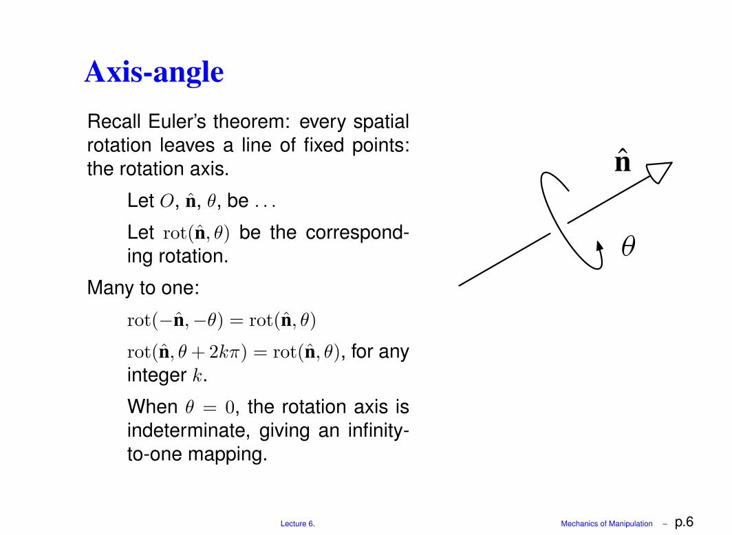
Axis-angleRecall Euler’s theorem: every spatialrotation leaves a line of fixed points:the rotation axis.

Let O, n, θ, be . . .

Let rot(n, θ) be the correspond-ing rotation.

Many to one:

rot(−n,−θ) = rot(n, θ)

rot(n, θ + 2kπ) = rot(n, θ), for anyinteger k.

When θ = 0, the rotation axis isindeterminate, giving an infinity-to-one mapping.

n


RepresentationWhat do we want from a representation? For a start:

• Rotate points;Rodrigues’s formula

• Compose rotations;Using axis-angle? Ugh.

• (Convert to other representations.)


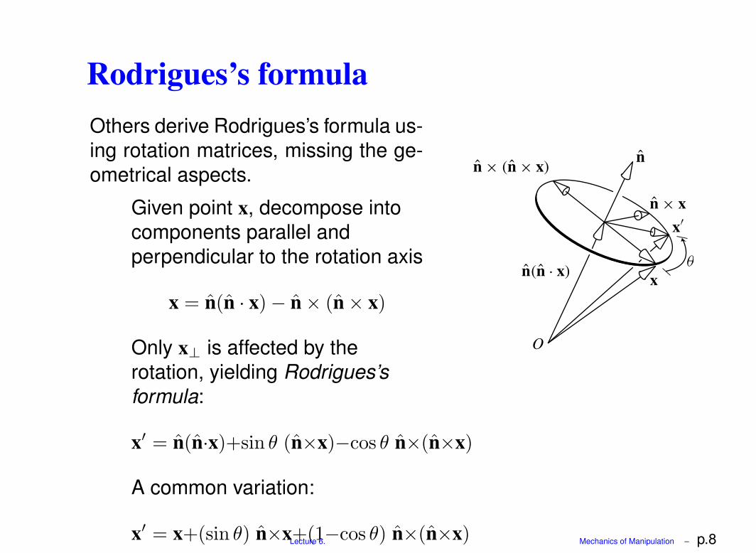
Rodrigues’s formulaOthers derive Rodrigues’s formula us-ing rotation matrices, missing the ge-ometrical aspects.

Given point x, decompose intocomponents parallel andperpendicular to the rotation axis

x = n(n · x) − n × (n × x)

Only x⊥ is affected by therotation, yielding Rodrigues’sformula:

x′ = n(n·x)+sin θ (n×x)−cos θ n×(n×x)

A common variation:

x′ = x+(sin θ) n×x+(1−cos θ) n×(n×x)

n n x

n n x

n

n xx

x

O


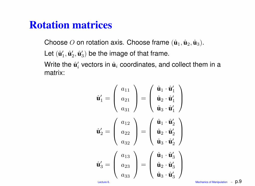
Rotation matricesChoose O on rotation axis. Choose frame (u1, u2, u3).

Let (u′

1, u′

2, u′

3) be the image of that frame.

Write the u′

i vectors in ui coordinates, and collect them in amatrix:

u′

1=

a11

a21

a31

=

u1 · u′

1

u2 · u′

1

u3 · u′

1

u′

2=

a12

a22

a32

=

u1 · u′

2

u2 · u′

2

u3 · u′

2

u′

3=

a13

a23

a33

=

u1 · u′

3

u2 · u′

3

u3 · u′

3

A = (aij) = (u′

1|u′

2|u′

3)


So many numbersA rotation matrix has nine numbers,

but spatial rotations have only three degrees of freedom,

leaving six excess numbers . . .

There are six constraints that hold among the nine numbers.

|u′

1| = |u′

2| = |u′

3| = 1

u′

3= u′

1× u′

2

i.e. the u′

i are unit vectors forming a right-handed coordinatesystem.

Such matrices are called orthonormal or rotation matrices.


Rotating a pointLet (x1, x2, x3) be coordinates of x in frame (u1, u2, u3).

Then x′ is given by the same coordinates taken in the (u′

1, u′

2, u′

3)

frame:

x′ =x1u′

1+ x2u′

2+ x3u′

3

=x1Au1 + x2Au2 + x3Au3

=A(x1u1 + x2u2 + x3u3)

=Ax

So rotating a point is implemented by ordinary matrixmultiplication.


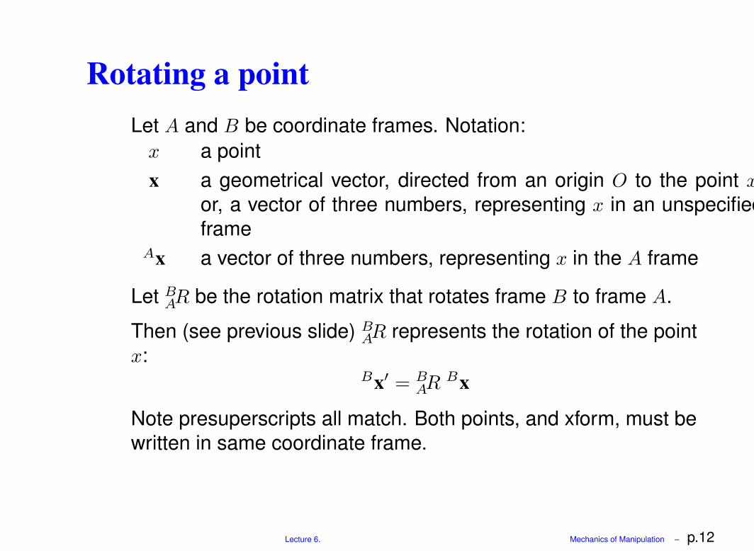
Rotating a pointLet A and B be coordinate frames. Notation:

x a pointx a geometrical vector, directed from an origin O to the point x;

or, a vector of three numbers, representing x in an unspecifiedframe

Ax a vector of three numbers, representing x in the A frame

Let BAR be the rotation matrix that rotates frame B to frame A.

Then (see previous slide) BAR represents the rotation of the point

x:Bx′ = B

AR Bx

Note presuperscripts all match. Both points, and xform, must bewritten in same coordinate frame.


Coordinate transformThere is another use for B

AR:Ax and Bx represent the same point, in frames A and B resp.

To transform from A to B:

Bx = BAR Ax

For coord xform, matrix subscript and vector superscript“cancel”.

Rotation from B to A is the same as coordinate transform from A to

B.


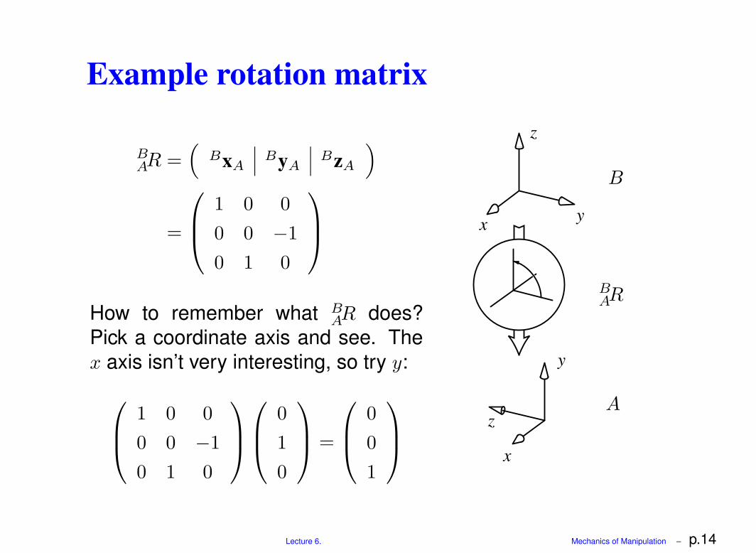
Example rotation matrix

BAR =

(

BxAByA

BzA

)

=

1 0 0

0 0 −1

0 1 0

How to remember what BAR does?

Pick a coordinate axis and see. Thex axis isn’t very interesting, so try y:

1 0 0

0 0 −1

0 1 0

0

1

0

=

0

0

1


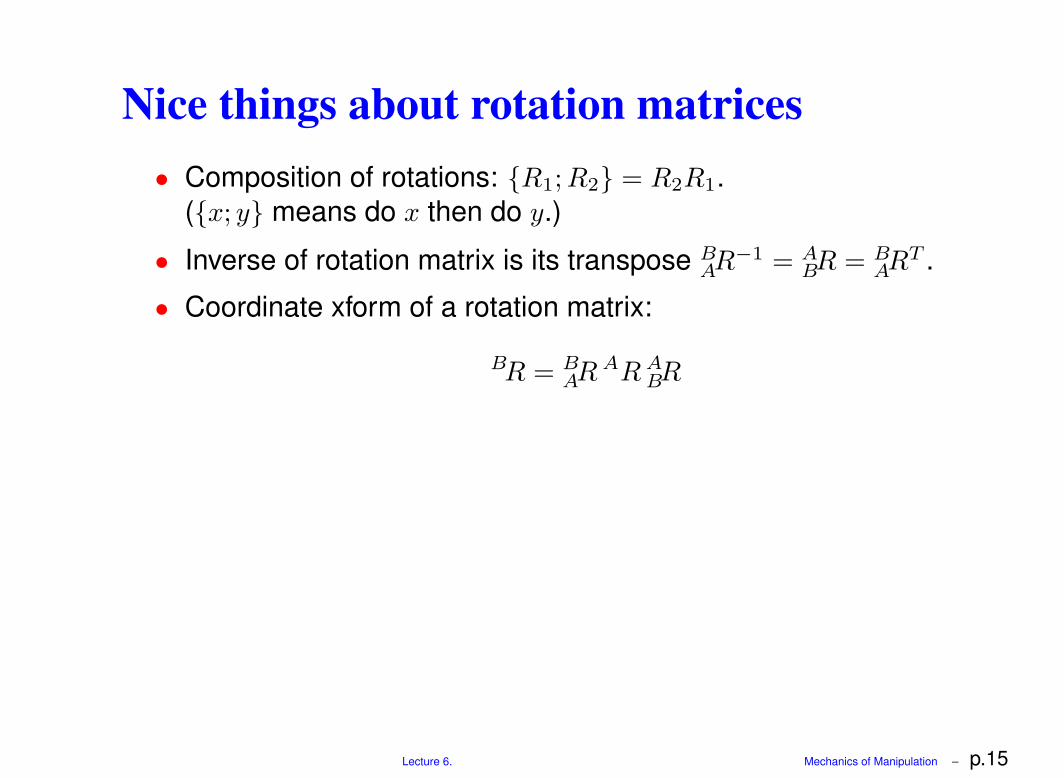
Nice things about rotation matrices• Composition of rotations: {R1; R2} = R2R1.

({x; y} means do x then do y.)

• Inverse of rotation matrix is its transpose BAR−1 = A

BR = BART .

• Coordinate xform of a rotation matrix:

BR = BAR AR A

BR


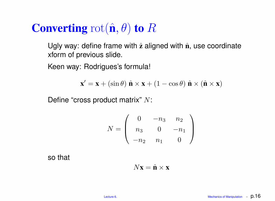
Converting rot(n, θ) to R

Ugly way: define frame with z aligned with n, use coordinatexform of previous slide.

Keen way: Rodrigues’s formula!

x′ = x + (sin θ) n × x + (1 − cos θ) n × (n × x)

Define “cross product matrix” N :

N =

0 −n3 n2

n3 0 −n1

−n2 n1 0

so thatNx = n × x


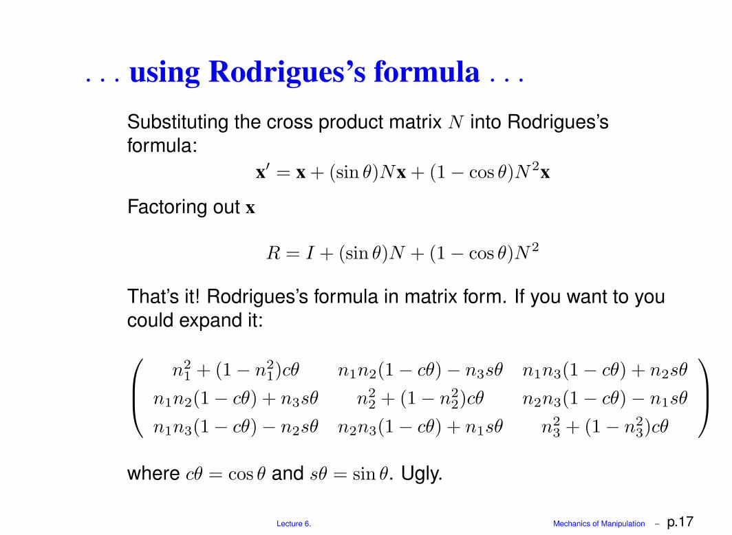
. . . using Rodrigues’s formula . . .

Substituting the cross product matrix N into Rodrigues’sformula:

x′ = x + (sin θ)Nx + (1 − cos θ)N 2x

Factoring out x

R = I + (sin θ)N + (1 − cos θ)N 2

That’s it! Rodrigues’s formula in matrix form. If you want to youcould expand it:

n2

1+ (1 − n2

1)cθ n1n2(1 − cθ) − n3sθ n1n3(1 − cθ) + n2sθ

n1n2(1 − cθ) + n3sθ n2

2+ (1 − n2

2)cθ n2n3(1 − cθ) − n1sθ

n1n3(1 − cθ) − n2sθ n2n3(1 − cθ) + n1sθ n2

3+ (1 − n2

3)cθ

where cθ = cos θ and sθ = sin θ. Ugly.


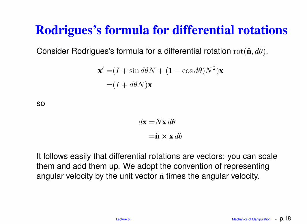
Rodrigues’s formula for differential rotationsConsider Rodrigues’s formula for a differential rotation rot(n, dθ).

x′ =(I + sin dθN + (1 − cos dθ)N 2)x

=(I + dθN)x

so

dx =Nx dθ

=n × x dθ

It follows easily that differential rotations are vectors: you can scalethem and add them up. We adopt the convention of representingangular velocity by the unit vector n times the angular velocity.


Converting from R to rot(n, θ) . . .

Problem: n isn’t defined for θ = 0.

We will do it indirectly. Convert R to a unit quaternion (nextlecture), then to axis-angle.


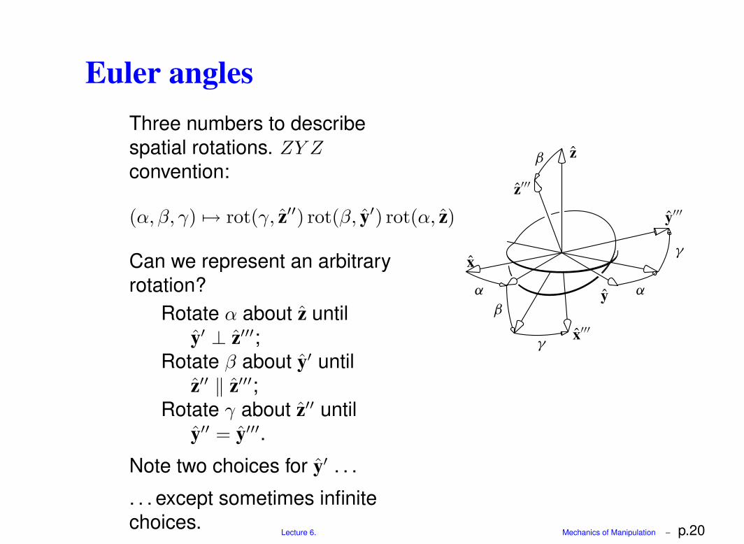
Euler anglesThree numbers to describespatial rotations. ZY Z

convention:

(α, β, γ) 7→ rot(γ, z′′) rot(β, y′) rot(α, z)

Can we represent an arbitraryrotation?

Rotate α about z untily′ ⊥ z′′′;

Rotate β about y′ untilz′′ ‖ z′′′;

Rotate γ about z′′ untily′′ = y′′′.

Note two choices for y′ . . .

. . . except sometimes infinitechoices.

x

x

y

y

z

z


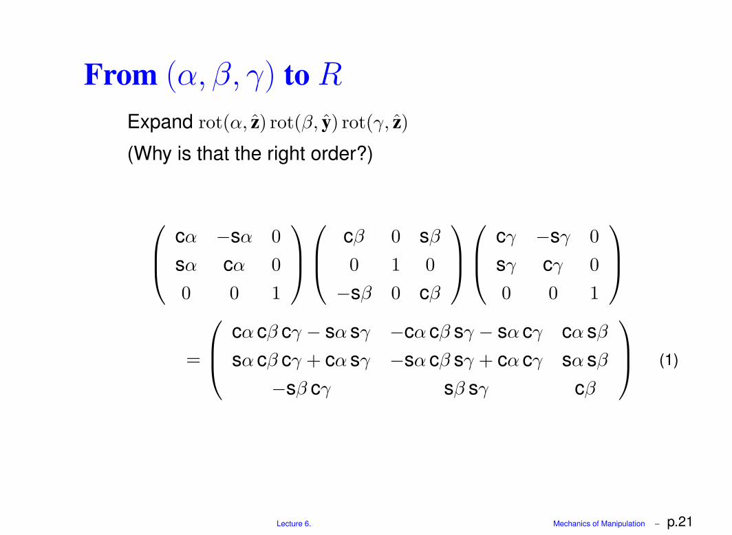
From (α, β, γ) to R

Expand rot(α, z) rot(β, y) rot(γ, z)

(Why is that the right order?)

cα −sα 0

sα cα 0

0 0 1

cβ 0 sβ

0 1 0

−sβ 0 cβ

cγ −sγ 0

sγ cγ 0

0 0 1

=

cα cβ cγ − sα sγ −cα cβ sγ − sα cγ cα sβ

sα cβ cγ + cα sγ −sα cβ sγ + cα cγ sα sβ

−sβ cγ sβ sγ cβ

(1)


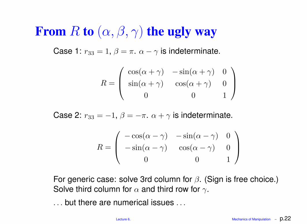
From R to (α, β, γ) the ugly wayCase 1: r33 = 1, β = π. α − γ is indeterminate.

R =

cos(α + γ) − sin(α + γ) 0

sin(α + γ) cos(α + γ) 0

0 0 1

Case 2: r33 = −1, β = −π. α + γ is indeterminate.

R =

− cos(α − γ) − sin(α − γ) 0

− sin(α − γ) cos(α − γ) 0

0 0 1

For generic case: solve 3rd column for β. (Sign is free choice.)Solve third column for α and third row for γ.

. . . but there are numerical issues . . .


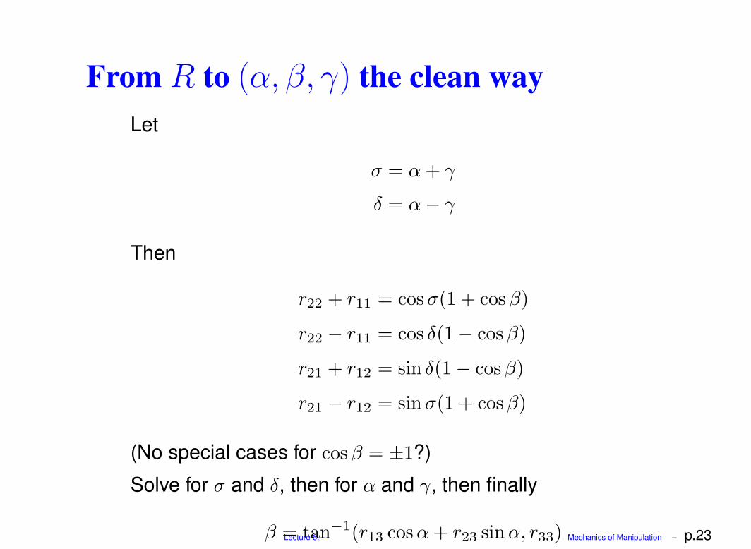
From R to (α, β, γ) the clean wayLet

σ = α + γ

δ = α − γ

Then

r22 + r11 = cos σ(1 + cosβ)

r22 − r11 = cos δ(1 − cosβ)

r21 + r12 = sin δ(1 − cosβ)

r21 − r12 = sin σ(1 + cosβ)

(No special cases for cosβ = ±1?)

Solve for σ and δ, then for α and γ, then finally

β = tan−1(r13 cos α + r23 sinα, r33)Lecture 6. Mechanics of Manipulation – p.23

Next: Quaternions.

Chapter 1 Manipulation 11.1 Case 1: Manipulation by a human 11.2 Case 2: An automated assembly system 31.3 Issues in manipulation 51.4 A taxonomy of manipulation techniques 71.5 Bibliographic notes 8

Exercises 8

Chapter 2 Kinematics 112.1 Preliminaries 112.2 Planar kinematics 152.3 Spherical kinematics 202.4 Spatial kinematics 222.5 Kinematic constraint 252.6 Kinematic mechanisms 342.7 Bibliographic notes 36

Exercises 37

Chapter 3 Kinematic Representation 413.1 Representation of spatial rotations 413.2 Representation of spatial displacements 583.3 Kinematic constraints 683.4 Bibliographic notes 72

Exercises 72

Chapter 4 Kinematic Manipulation 774.1 Path planning 774.2 Path planning for nonholonomic systems 844.3 Kinematic models of contact 864.4 Bibliographic notes 88

Exercises 88

Chapter 5 Rigid Body Statics 935.1 Forces acting on rigid bodies 935.2 Polyhedral convex cones 995.3 Contact wrenches and wrench cones 1025.4 Cones in velocity twist space 1045.5 The oriented plane 1055.6 Instantaneous centers and Reuleaux’s method 1095.7 Line of force; moment labeling 1105.8 Force dual 1125.9 Summary 1175.10 Bibliographic notes 117

Exercises 118

Chapter 6 Friction 1216.1 Coulomb’s Law 1216.2 Single degree-of-freedom problems 1236.3 Planar single contact problems 1266.4 Graphical representation of friction cones 1276.5 Static equilibrium problems 1286.6 Planar sliding 1306.7 Bibliographic notes 139

Exercises 139

Chapter 7 Quasistatic Manipulation 1437.1 Grasping and fixturing 1437.2 Pushing 1477.3 Stable pushing 1537.4 Parts orienting 1627.5 Assembly 1687.6 Bibliographic notes 173

Exercises 175

Chapter 8 Dynamics 1818.1 Newton’s laws 1818.2 A particle in three dimensions 1818.3 Moment of force; moment of momentum 1838.4 Dynamics of a system of particles 1848.5 Rigid body dynamics 1868.6 The angular inertia matrix 1898.7 Motion of a freely rotating body 1958.8 Planar single contact problems 1978.9 Graphical methods for the plane 2038.10 Planar multiple-contact problems 2058.11 Bibliographic notes 207

Exercises 208

Chapter 9 Impact 2119.1 A particle 2119.2 Rigid body impact 2179.3 Bibliographic notes 223

Exercises 223

Chapter 10 Dynamic Manipulation 22510.1 Quasidynamic manipulation 22510.2 Brie� y dynamic manipulation 22910.3 Continuously dynamic manipulation 23010.4 Bibliographic notes 232

Exercises 235

Appendix A Infinity 237


Documents

6. Representing Rotation - Computer Sciencetrink/Courses/RobotManipulation/lectures/lecture6.pdf · Lecture 6. Representing Rotation. Chapter 1 Manipulation 1 ... 6.4 Graphical representation