Embed Size (px)
Citation preview

6
Metric Spaces
Definition 6.1. A function d : X ×X → [0,∞) is called a metric if1. (Symmetry) d(x, y) = d(y, x) for all x, y ∈ X2. (Non-degenerate) d(x, y) = 0 if and only if x = y ∈ X3. (Triangle inequality) d(x, z) ≤ d(x, y) + d(y, z) for all x, y, z ∈ X.
As primary examples, any normed space (X, k·k) (see Definition 5.1) is ametric space with d(x, y) := kx− yk . Thus the space p(µ) (as in Theorem5.2) is a metric space for all p ∈ [1,∞]. Also any subset of a metric spaceis a metric space. For example a surface Σ in R3 is a metric space with thedistance between two points on Σ being the usual distance in R3.
Definition 6.2. Let (X,d) be a metric space. The open ball B(x, δ) ⊂ Xcentered at x ∈ X with radius δ > 0 is the set
B(x, δ) := {y ∈ X : d(x, y) < δ}.
We will often also write B(x, δ) as Bx(δ). We also define the closed ballcentered at x ∈ X with radius δ > 0 as the set Cx(δ) := {y ∈ X : d(x, y) ≤ δ}.Definition 6.3. A sequence {xn}∞n=1 in a metric space (X, d) is said to beconvergent if there exists a point x ∈ X such that limn→∞ d(x, xn) = 0. Inthis case we write limn→∞ xn = x of xn → x as n→∞.
Exercise 6.1. Show that x in Definition 6.3 is necessarily unique.
Definition 6.4. A set E ⊂ X is bounded if E ⊂ B (x,R) for some x ∈ Xand R < ∞. A set F ⊂ X is closed iff every convergent sequence {xn}∞n=1which is contained in F has its limit back in F. A set V ⊂ X is open iff V c
is closed. We will write F @ X to indicate the F is a closed subset of X andV ⊂o X to indicate the V is an open subset of X. We also let τd denote thecollection of open subsets of X relative to the metric d.

50 6 Metric Spaces
Definition 6.5. A subset A ⊂ X is a neighborhood of x if there exists anopen set V ⊂o X such that x ∈ V ⊂ A. We will say that A ⊂ X is an openneighborhood of x if A is open and x ∈ A.
Exercise 6.2. Let F be a collection of closed subsets of X, show ∩F :=∩F∈FF is closed. Also show that finite unions of closed sets are closed, i.e. if{Fk}nk=1 are closed sets then ∪nk=1Fk is closed. (By taking complements, thisshows that the collection of open sets, τd, is closed under finite intersectionsand arbitrary unions.)
The following “continuity” facts of the metric d will be used frequently inthe remainder of this book.
Lemma 6.6. For any non empty subset A ⊂ X, let dA(x) := inf{d(x, a)|a ∈A}, then
|dA(x)− dA(y)| ≤ d(x, y) ∀x, y ∈ X (6.1)
and in particular if xn → x in X then dA (xn)→ dA (x) as n→∞. Moreoverthe set Fε := {x ∈ X|dA(x) ≥ ε} is closed in X.
Proof. Let a ∈ A and x, y ∈ X, then
d(x, a) ≤ d(x, y) + d(y, a).
Take the inf over a in the above equation shows that
dA(x) ≤ d(x, y) + dA(y) ∀x, y ∈ X.
Therefore, dA(x)−dA(y) ≤ d(x, y) and by interchanging x and y we also havethat dA(y)− dA(x) ≤ d(x, y) which implies Eq. (6.1). If xn → x ∈ X, then byEq. (6.1),
|dA(x)− dA(xn)| ≤ d(x, xn)→ 0 as n→∞so that limn→∞ dA (xn) = dA (x) . Now suppose that {xn}∞n=1 ⊂ Fε andxn → x in X, then
dA (x) = limn→∞ dA (xn) ≥ ε
since dA (xn) ≥ ε for all n. This shows that x ∈ Fε and hence Fε is closed.
Corollary 6.7. The function d satisfies,
|d(x, y)− d(x0, y0)| ≤ d(y, y0) + d(x, x0).
In particular d : X × X → [0,∞) is “continuous” in the sense that d(x, y)is close to d(x0, y0) if x is close to x0 and y is close to y0. (The notion ofcontinuity will be developed shortly.)

6.1 Continuity 51
Proof. By Lemma 6.6 for single point sets and the triangle inequality for theabsolute value of real numbers,
|d(x, y)− d(x0, y0)| ≤ |d(x, y)− d(x, y0)|+ |d(x, y0)− d(x0, y0)|≤ d(y, y0) + d(x, x0).
Example 6.8. Let x ∈ X and δ > 0, then Cx (δ) and Bx (δ)c are closed subsets
of X. For example if {yn}∞n=1 ⊂ Cx (δ) and yn → y ∈ X, then d (yn, x) ≤ δ forall n and using Corollary 6.7 it follows d (y, x) ≤ δ, i.e. y ∈ Cx (δ) . A similarproof shows Bx (δ)
c is open, see Exercise 6.3.
Exercise 6.3. Show that V ⊂ X is open iff for every x ∈ V there is a δ > 0such that Bx(δ) ⊂ V. In particular show Bx(δ) is open for all x ∈ X andδ > 0. Hint: by definition V is not open iff V c is not closed.
Lemma 6.9 (Approximating open sets from the inside by closedsets). Let A be a closed subset of X and Fε := {x ∈ X|dA(x) ≥ ε} @ Xbe as in Lemma 6.6. Then Fε ↑ Ac as ε ↓ 0.Proof. It is clear that dA(x) = 0 for x ∈ A so that Fε ⊂ Ac for each ε > 0 andhence ∪ε>0Fε ⊂ Ac. Now suppose that x ∈ Ac ⊂o X. By Exercise 6.3 thereexists an ε > 0 such that Bx(ε) ⊂ Ac, i.e. d(x, y) ≥ ε for all y ∈ A. Hencex ∈ Fε and we have shown that Ac ⊂ ∪ε>0Fε. Finally it is clear that Fε ⊂ Fε0whenever ε0 ≤ ε.
Definition 6.10. Given a set A contained a metric space X, let A ⊂ X bethe closure of A defined by
A := {x ∈ X : ∃ {xn} ⊂ A 3 x = limn→∞xn}.
That is to say A contains all limit points of A. We say A is dense in X ifA = X, i.e. every element x ∈ X is a limit of a sequence of elements from A.
Exercise 6.4. Given A ⊂ X, show A is a closed set and in fact
A = ∩{F : A ⊂ F ⊂ X with F closed}. (6.2)
That is to say A is the smallest closed set containing A.
6.1 Continuity
Suppose that (X, ρ) and (Y, d) are two metric spaces and f : X → Y is afunction.

52 6 Metric Spaces
Definition 6.11. A function f : X → Y is continuous at x ∈ X if for allε > 0 there is a δ > 0 such that
d(f(x), f(x0)) < ε provided that ρ(x, x0) < δ. (6.3)
The function f is said to be continuous if f is continuous at all points x ∈ X.
The following lemma gives two other characterizations of continuity of afunction at a point.
Lemma 6.12 (Local Continuity Lemma). Suppose that (X, ρ) and (Y, d)are two metric spaces and f : X → Y is a function defined in a neighborhoodof a point x ∈ X. Then the following are equivalent:
1. f is continuous at x ∈ X.2. For all neighborhoods A ⊂ Y of f(x), f−1(A) is a neighborhood of x ∈ X.3. For all sequences {xn}∞n=1 ⊂ X such that x = limn→∞ xn, {f(xn)} isconvergent in Y and
limn→∞ f(xn) = f
³limn→∞xn
´.
Proof. 1 =⇒ 2. If A ⊂ Y is a neighborhood of f (x) , there exists ε > 0 suchthat Bf(x) (ε) ⊂ A and because f is continuous there exists a δ > 0 such thatEq. (6.3) holds. Therefore
Bx (δ) ⊂ f−1¡Bf(x) (ε)
¢ ⊂ f−1 (A)
showing f−1 (A) is a neighborhood of x.2 =⇒ 3. Suppose that {xn}∞n=1 ⊂ X and x = limn→∞ xn. Then for
any ε > 0, Bf(x) (ε) is a neighborhood of f (x) and so f−1¡Bf(x) (ε)
¢is a
neighborhood of x which must containing Bx (δ) for some δ > 0. Becausexn → x, it follows that xn ∈ Bx (δ) ⊂ f−1
¡Bf(x) (ε)
¢for a.a. n and this
implies f (xn) ∈ Bf(x) (ε) for a.a. n, i.e. d(f(x), f (xn)) < ε for a.a. n. Sinceε > 0 is arbitrary it follows that limn→∞ f (xn) = f (x) .3. =⇒ 1. We will show not 1. =⇒ not 3. If f is not continuous at x,
there exists an ε > 0 such that for all n ∈ N there exists a point xn ∈ X withρ (xn, x) <
1n yet d (f (xn) , f (x)) ≥ ε. Hence xn → x as n → ∞ yet f (xn)
does not converge to f (x) .Here is a global version of the previous lemma.
Lemma 6.13 (Global Continuity Lemma). Suppose that (X, ρ) and (Y, d)are two metric spaces and f : X → Y is a function defined on all of X. Thenthe following are equivalent:
1. f is continuous.2. f−1(V ) ∈ τρ for all V ∈ τd, i.e. f−1(V ) is open in X if V is open in Y.3. f−1(C) is closed in X if C is closed in Y.

6.2 Completeness in Metric Spaces 53
4. For all convergent sequences {xn} ⊂ X, {f(xn)} is convergent in Y and
limn→∞ f(xn) = f
³limn→∞xn
´.
Proof. Since f−1 (Ac) =£f−1 (A)
¤c, it is easily seen that 2. and 3. are equiv-
alent. So because of Lemma 6.12 it only remains to show 1. and 2. are equiv-alent. If f is continuous and V ⊂ Y is open, then for every x ∈ f−1 (V ) ,V is a neighborhood of f (x) and so f−1 (V ) is a neighborhood of x. Hencef−1 (V ) is a neighborhood of all of its points and from this and Exercise 6.3it follows that f−1 (V ) is open. Conversely if x ∈ X and A ⊂ Y is a neigh-borhood of f (x) , then there exists V ⊂o X such that f (x) ∈ V ⊂ A. Hencex ∈ f−1 (V ) ⊂ f−1 (A) and by assumption f−1 (V ) is open showing f−1 (A)is a neighborhood of x. Therefore f is continuous at x and since x ∈ X wasarbitrary, f is continuous.
Example 6.14. The function dA defined in Lemma 6.6 is continuous for eachA ⊂ X. In particular, if A = {x} , it follows that y ∈ X → d(y, x) is continuousfor each x ∈ X.
Exercise 6.5. Use Example 6.14 and Lemma 6.13 to recover the results ofExample 6.8.
The next result shows that there are lots of continuous functions on ametric space (X,d) .
Lemma 6.15 (Urysohn’s Lemma for Metric Spaces). Let (X, d) be ametric space and suppose that A and B are two disjoint closed subsets of X.Then
f(x) =dB(x)
dA(x) + dB(x)for x ∈ X (6.4)
defines a continuous function, f : X → [0, 1], such that f(x) = 1 for x ∈ Aand f(x) = 0 if x ∈ B.
Proof. By Lemma 6.6, dA and dB are continuous functions on X. Since A andB are closed, dA(x) > 0 if x /∈ A and dB(x) > 0 if x /∈ B. Since A ∩ B = ∅,dA(x) + dB(x) > 0 for all x and (dA + dB)
−1 is continuous as well. Theremaining assertions about f are all easy to verify.Sometimes Urysohn’s lemma will be use in the following form. Suppose
F ⊂ V ⊂ X with F being closed and V being open, then there exists f ∈C (X, [0, 1])) such that f = 1 on F while f = 0 on V c. This of course followsfrom Lemma 6.15 by taking A = F and B = V c.
6.2 Completeness in Metric Spaces
Definition 6.16 (Cauchy sequences). A sequence {xn}∞n=1 in a metricspace (X, d) is Cauchy provided that

54 6 Metric Spaces
limm,n→∞ d(xn, xm) = 0.
Exercise 6.6. Show that convergent sequences are always Cauchy sequences.The converse is not always true. For example, let X = Q be the set of rationalnumbers and d(x, y) = |x − y|. Choose a sequence {xn}∞n=1 ⊂ Q which con-verges to
√2 ∈ R, then {xn}∞n=1 is (Q, d) — Cauchy but not (Q, d) — convergent.
The sequence does converge in R however.
Definition 6.17. A metric space (X, d) is complete if all Cauchy sequencesare convergent sequences.
Exercise 6.7. Let (X,d) be a complete metric space. Let A ⊂ X be a subsetof X viewed as a metric space using d|A×A. Show that (A, d|A×A) is completeiff A is a closed subset of X.
Example 6.18. Examples 2. — 4. of complete metric spaces will be verified inChapter 7 below.
1. X = R and d(x, y) = |x− y|, see Theorem 3.8 above.2. X = Rn and d(x, y) = kx− yk2 =
Pni=1(xi − yi)
2.3. X = p(µ) for p ∈ [1,∞] and any weight function µ : X → (0,∞).4. X = C([0, 1],R) — the space of continuous functions from [0, 1] to R and
d(f, g) := maxt∈[0,1]
|f(t)− g(t)|.
This is a special case of Lemma 7.3 below.5. Let X = C([0, 1],R) and
d(f, g) :=
Z 1
0
|f(t)− g(t)| dt.
You are asked in Exercise 7.14 to verify that (X,d) is a metric space whichis not complete.
Exercise 6.8 (Completions of Metric Spaces). Suppose that (X, d) isa (not necessarily complete) metric space. Using the following outline showthere exists a complete metric space
¡X, d
¢and an isometric map i : X → X
such that i (X) is dense in X, see Definition 6.10.
1. Let C denote the collection of Cauchy sequences a = {an}∞n=1 ⊂ X. Giventwo element a, b ∈ C show
dC (a, b) := limn→∞ d (an, bn) exists,
dC (a, b) ≥ 0 for all a, b ∈ C and dC satisfies the triangle inequality,
dC (a, c) ≤ dC (a, b) + dC (b, c) for all a, b, c ∈ C.Thus (C, dC) would be a metric space if it were true that dC(a, b) = 0 iffa = b. This however is false, for example if an = bn for all n ≥ 100, thendC(a, b) = 0 while a need not equal b.

6.3 Supplementary Remarks 55
2. Define two elements a, b ∈ C to be equivalent (write a ∼ b) wheneverdC(a, b) = 0. Show “ ∼ ” is an equivalence relation on C and thatdC (a0, b0) = dC (a, b) if a ∼ a0 and b ∼ b0. (Hint: see Corollary 6.7.)
3. Given a ∈ C let a := {b ∈ C : b ∼ a} denote the equivalence class contain-ing a and let X := {a : a ∈ C} denote the collection of such equivalenceclasses. Show that d
¡a, b¢:= dC (a, b) is well defined on X × X and verify¡
X, d¢is a metric space.
4. For x ∈ X let i (x) = a where a is the constant sequence, an = x for all n.Verify that i : X → X is an isometric map and that i (X) is dense in X.
5. Verify¡X, d
¢is complete. Hint: if {a(m)}∞m=1 is a Cauchy sequence in X
choose bm ∈ X such that d (i (bm) , a(m)) ≤ 1/m. Then show a(m) → bwhere b = {bm}∞m=1 .
6.3 Supplementary Remarks
6.3.1 Word of Caution
Example 6.19. Let (X, d) be a metric space. It is always true that Bx(ε) ⊂Cx(ε) since Cx(ε) is a closed set containing Bx(ε). However, it is not alwaystrue that Bx(ε) = Cx(ε). For example let X = {1, 2} and d(1, 2) = 1, thenB1(1) = {1} , B1(1) = {1} while C1(1) = X. For another counter example,take
X =©(x, y) ∈ R2 : x = 0 or x = 1ª
with the usually Euclidean metric coming from the plane. Then
B(0,0)(1) =©(0, y) ∈ R2 : |y| < 1ª ,
B(0,0)(1) =©(0, y) ∈ R2 : |y| ≤ 1ª , while
C(0,0)(1) = B(0,0)(1) ∪ {(0, 1)} .In spite of the above examples, Lemmas 6.20 and 6.21 below shows that
for certain metric spaces of interest it is true that Bx(ε) = Cx(ε).
Lemma 6.20. Suppose that (X, |·|) is a normed vector space and d is themetric on X defined by d(x, y) = |x− y| . Then
Bx(ε) = Cx(ε) and
bd(Bx(ε)) = {y ∈ X : d(x, y) = ε}.where the boundary operation, bd(·) is defined in Definition 10.30 below.Proof. We must show that C := Cx(ε) ⊂ Bx(ε) =: B. For y ∈ C, let v = y−x,then
|v| = |y − x| = d(x, y) ≤ ε.
Let αn = 1 − 1/n so that αn ↑ 1 as n → ∞. Let yn = x + αnv, thend(x, yn) = αnd(x, y) < ε, so that yn ∈ Bx(ε) and d(y, yn) = 1 − αn → 0 asn→∞. This shows that yn → y as n→∞ and hence that y ∈ B.

56 6 Metric Spaces
ε
δ
Fig. 6.1. An almost length minimizing curve joining x to y.
6.3.2 Riemannian Metrics
This subsection is not completely self contained and may safely be skipped.
Lemma 6.21. Suppose that X is a Riemannian (or sub-Riemannian) mani-fold and d is the metric on X defined by
d(x, y) = inf { (σ) : σ(0) = x and σ(1) = y}where (σ) is the length of the curve σ. We define (σ) = ∞ if σ is notpiecewise smooth.Then
Bx(ε) = Cx(ε) and
bd(Bx(ε)) = {y ∈ X : d(x, y) = ε}where the boundary operation, bd(·) is defined in Definition 10.30 below.Proof. Let C := Cx(ε) ⊂ Bx(ε) =: B. We will show that C ⊂ B by showingBc ⊂ Cc. Suppose that y ∈ Bc and choose δ > 0 such that By(δ) ∩ B = ∅. Inparticular this implies that
By(δ) ∩Bx(ε) = ∅.We will finish the proof by showing that d(x, y) ≥ ε + δ > ε and hencethat y ∈ Cc. This will be accomplished by showing: if d(x, y) < ε + δ thenBy(δ) ∩Bx(ε) 6= ∅.If d(x, y) < max(ε, δ) then either x ∈ By(δ) or y ∈ Bx(ε). In either case
By(δ) ∩ Bx(ε) 6= ∅. Hence we may assume that max(ε, δ) ≤ d(x, y) < ε + δ.Let α > 0 be a number such that
max(ε, δ) ≤ d(x, y) < α < ε+ δ
and choose a curve σ from x to y such that (σ) < α. Also choose 0 < δ0 < δsuch that 0 < α−δ0 < ε which can be done since α−δ < ε. Let k(t) = d(y, σ(t))a continuous function on [0, 1] and therefore k([0, 1]) ⊂ R is a connected

6.4 Exercises 57
set which contains 0 and d(x, y). Therefore there exists t0 ∈ [0, 1] such thatd(y, σ(t0)) = k(t0) = δ0. Let z = σ(t0) ∈ By(δ) then
d(x, z) ≤ (σ|[0,t0]) = (σ)− (σ|[t0,1]) < α− d(z, y) = α− δ0 < ε
and therefore z ∈ Bx(ε) ∩Bx(δ) 6= ∅.Remark 6.22. Suppose again that X is a Riemannian (or sub-Riemannian)manifold and
d(x, y) = inf { (σ) : σ(0) = x and σ(1) = y} .Let σ be a curve from x to y and let ε = (σ)− d(x, y). Then for all 0 ≤ u <v ≤ 1,
d(σ(u), σ(v)) ≤ (σ|[u,v]) + ε.
So if σ is within ε of a length minimizing curve from x to y that σ|[u,v] iswithin ε of a length minimizing curve from σ(u) to σ(v). In particular ifd(x, y) = (σ) then d(σ(u), σ(v)) = (σ|[u,v]) for all 0 ≤ u < v ≤ 1, i.e. if σis a length minimizing curve from x to y that σ|[u,v] is a length minimizingcurve from σ(u) to σ(v).To prove these assertions notice that
d(x, y) + ε = (σ) = (σ|[0,u]) + (σ|[u,v]) + (σ|[v,1])≥ d(x, σ(u)) + (σ|[u,v]) + d(σ(v), y)
and therefore
(σ|[u,v]) ≤ d(x, y) + ε− d(x, σ(u))− d(σ(v), y)
≤ d(σ(u), σ(v)) + ε.
6.4 Exercises
Exercise 6.9. Let (X,d) be a metric space. Suppose that {xn}∞n=1 ⊂ X is asequence and set εn := d(xn, xn+1). Show that for m > n that
d(xn, xm) ≤m−1Xk=n
εk ≤∞Xk=n
εk.
Conclude from this that if∞Xk=1
εk =∞Xn=1
d(xn, xn+1) <∞
then {xn}∞n=1 is Cauchy. Moreover, show that if {xn}∞n=1 is a convergentsequence and x = limn→∞ xn then
d(x, xn) ≤∞Xk=n
εk.

58 6 Metric Spaces
Exercise 6.10. Show that (X,d) is a complete metric space iff every sequence{xn}∞n=1 ⊂ X such that
P∞n=1 d(xn, xn+1) < ∞ is a convergent sequence in
X. You may find it useful to prove the following statements in the course ofthe proof.
1. If {xn} is Cauchy sequence, then there is a subsequence yj := xnj suchthat
P∞j=1 d(yj+1, yj) <∞.
2. If {xn}∞n=1 is Cauchy and there exists a subsequence yj := xnj of {xn}such that x = limj→∞ yj exists, then limn→∞ xn also exists and is equalto x.
Exercise 6.11. Suppose that f : [0,∞) → [0,∞) is a C2 — function suchthat f(0) = 0, f 0 > 0 and f 00 ≤ 0 and (X, ρ) is a metric space. Show thatd(x, y) = f(ρ(x, y)) is a metric on X. In particular show that
d(x, y) :=ρ(x, y)
1 + ρ(x, y)
is a metric on X. (Hint: use calculus to verify that f(a+ b) ≤ f(a) + f(b) forall a, b ∈ [0,∞).)Exercise 6.12. Let {(Xn, dn)}∞n=1 be a sequence of metric spaces, X :=Q∞
n=1Xn, and for x = (x(n))∞n=1 and y = (y(n))
∞n=1 in X let
d(x, y) =∞Xn=1
2−ndn(x(n), y(n))
1 + dn(x(n), y(n)).
Show:
1. (X, d) is a metric space,2. a sequence {xk}∞k=1 ⊂ X converges to x ∈ X iff xk(n) → x(n) ∈ Xn ask →∞ for each n ∈ N and
3. X is complete if Xn is complete for all n.
Exercise 6.13. Suppose (X,ρ) and (Y, d) are metric spaces and A is a densesubset of X.
1. Show that if F : X → Y and G : X → Y are two continuous functionssuch that F = G on A then F = G on X. Hint: consider the set C :={x ∈ X : F (x) = G (x)} .
2. Suppose f : A → Y is a function which is uniformly continuous, i.e. forevery ε > 0 there exists a δ > 0 such that
d (f (a) , f (b)) < ε for all a, b ∈ A with ρ (a, b) < δ.
Show there is a unique continuous function F : X → Y such that F = f onA. Hint: each point x ∈ X is a limit of a sequence consisting of elementsfrom A.
3. Let X = R = Y and A = Q ⊂ X, find a function f : Q→ R which iscontinuous on Q but does not extend to a continuous function on R.

7
Banach Spaces
Let (X, k·k) be a normed vector space and d (x, y) := kx− yk be the asso-ciated metric on X. We say {xn}∞n=1 ⊂ X converges to x ∈ X (and writelimn→∞ xn = x or xn → x) if
0 = limn→∞ d (x, xn) = lim
n→∞ kx− xnk .
Similarly {xn}∞n=1 ⊂ X is said to be a Cauchy sequence if
0 = limm,n→∞ d (xm, xn) = lim
m,n→∞ kxm − xnk .
Definition 7.1 (Banach space). A normed vector space (X, k·k) is a Ba-nach space if the associated metric space (X,d) is complete, i.e. all Cauchysequences are convergent.
Remark 7.2. Since kxk = d (x, 0) , it follows from Lemma 6.6 that k·k is acontinuous function on X and that
|kxk− kyk| ≤ kx− yk for all x, y ∈ X.
It is also easily seen that the vector addition and scalar multiplication arecontinuos on any normed space as the reader is asked to verify in Exercise7.7. These facts will often be used in the sequel without further mention.
7.1 Examples
Lemma 7.3. Suppose that X is a set then the bounded functions, ∞(X), onX is a Banach space with the norm
kfk = kfk∞ = supx∈X
|f(x)| .
Moreover if X is a metric space (more generally a topological space, see Chap-ter 10) the set BC(X) ⊂ ∞(X) = B(X) is closed subspace of ∞(X) andhence is also a Banach space.

60 7 Banach Spaces
Proof. Let {fn}∞n=1 ⊂ ∞(X) be a Cauchy sequence. Since for any x ∈ X, wehave
|fn(x)− fm(x)| ≤ kfn − fmk∞ (7.1)
which shows that {fn(x)}∞n=1 ⊂ F is a Cauchy sequence of numbers. Because F(F = R or C) is complete, f(x) := limn→∞ fn(x) exists for all x ∈ X. Passingto the limit n→∞ in Eq. (7.1) implies
|f(x)− fm(x)| ≤ lim infn→∞ kfn − fmk∞
and taking the supremum over x ∈ X of this inequality implies
kf − fmk∞ ≤ lim infn→∞ kfn − fmk∞ → 0 as m→∞
showing fm → f in ∞(X).For the second assertion, suppose that {fn}∞n=1 ⊂ BC(X) ⊂ ∞(X) and
fn → f ∈ ∞(X). We must show that f ∈ BC(X), i.e. that f is continuous.To this end let x, y ∈ X, then
|f(x)− f(y)| ≤ |f(x)− fn(x)|+ |fn(x)− fn(y)|+ |fn(y)− f(y)|≤ 2 kf − fnk∞ + |fn(x)− fn(y)| .
Thus if ε > 0, we may choose n large so that 2 kf − fnk∞ < ε/2 andthen for this n there exists an open neighborhood Vx of x ∈ X such that|fn(x)− fn(y)| < ε/2 for y ∈ Vx. Thus |f(x)− f(y)| < ε for y ∈ Vx showingthe limiting function f is continuous.Here is an application of this theorem.
Theorem 7.4 (Metric Space Tietze Extension Theorem). Let (X, d)be a metric space, D be a closed subset of X, −∞ < a < b < ∞ and f ∈C(D, [a, b]). (Here we are viewing D as a metric space with metric dD :=dD×D.) Then there exists F ∈ C(X, [a, b]) such that F |D = f.
Proof. 1. By scaling and translation (i.e. by replacing f by (b− a)−1 (f − a)),it suffices to prove Theorem 7.4 with a = 0 and b = 1.
2. Suppose α ∈ (0, 1] and f : D → [0, α] is continuous function. Let A :=f−1([0, 13α]) andB := f−1([23α, α]). By Lemma 6.15 there exists a functiong ∈ C(X, [0, α/3]) such that g = 0 on A and g = 1 on B. Letting g := α
3 g,we have g ∈ C(X, [0, α/3]) such that g = 0 on A and g = α/3 on B.Further notice that
0 ≤ f(x)− g(x) ≤ 23α for all x ∈ D.
3. Now suppose f : D → [0, 1] is a continuous function as in step 1. Letg1 ∈ C(X, [0, 1/3]) be as in step 2, see Figure 7.1. with α = 1 and letf1 := f − g1|D ∈ C(D, [0, 2/3]). Apply step 2. with α = 2/3 and f = f1 to

7.1 Examples 61
find g2 ∈ C(X, [0, 1323 ]) such that f2 := f − (g1 + g2) |D ∈ C(D, [0,
¡23
¢2]).
Continue this way inductively to find gn ∈ C(X, [0, 13¡23
¢n−1]) such that
f −NXn=1
gn|D =: fN ∈ C(D, [0,
µ2
3
¶N]). (7.2)
4. Define F :=P∞
n=1 gn. Since
∞Xn=1
kgnk∞ ≤∞Xn=1
1
3
µ2
3
¶n−1=1
3
1
1− 23
= 1,
the series defining F is uniformly convergent so F ∈ C(X, [0, 1]). Passingto the limit in Eq. (7.2) shows f = F |D.
Fig. 7.1. Reducing f by subtracting off a globally defined function g1 ∈C¡X, [0, 1
3]¢.
Theorem 7.5 (Completeness of p(µ)). Let X be a set and µ : X → (0,∞)be a given function. Then for any p ∈ [1,∞], ( p(µ), k·kp) is a Banach space.Proof. We have already proved this for p =∞ in Lemma 7.3 so we now assumethat p ∈ [1,∞). Let {fn}∞n=1 ⊂ p(µ) be a Cauchy sequence. Since for anyx ∈ X,
|fn(x)− fm(x)| ≤ 1
µ(x)kfn − fmkp → 0 as m,n→∞
it follows that {fn(x)}∞n=1 is a Cauchy sequence of numbers and f(x) :=limn→∞ fn(x) exists for all x ∈ X. By Fatou’s Lemma,
62 7 Banach Spaces
kfn − fkpp =XX
µ · limm→∞ inf |fn − fm|p ≤ lim
m→∞ infXX
µ · |fn − fm|p
= limm→∞ inf kfn − fmkpp → 0 as n→∞.
This then shows that f = (f − fn) + fn ∈ p(µ) (being the sum of two p —
functions) and that fnp−→ f.
Remark 7.6. Let X be a set, Y be a Banach space and ∞(X,Y ) denote thebounded functions f : X → Y equipped with the norm
kfk = kfk∞ = supx∈X
kf(x)kY .
If X is a metric space (or a general topological space, see Chapter 10), letBC(X,Y ) denote those f ∈ ∞(X,Y ) which are continuous. The same proofused in Lemma 7.3 shows that ∞(X,Y ) is a Banach space and that BC(X,Y )is a closed subspace of ∞(X,Y ). Similarly, if 1 ≤ p <∞ we may define
p (X,Y ) =
f : X → Y : kfkp =ÃXx∈X
kf (x)kpY!1/p
<∞ .
The same proof as in Theorem 7.5 would then show that³
p (X,Y ) , k·kp´is
a Banach space.
7.2 Bounded Linear Operators Basics
Definition 7.7. Let X and Y be normed spaces and T : X → Y be a linearmap. Then T is said to be bounded provided there exists C < ∞ such thatkT (x)k ≤ CkxkX for all x ∈ X. We denote the best constant by kTk, i.e.
kTk = supx 6=0
kT (x)kkxk = sup
x6=0{kT (x)k : kxk = 1} .
The number kTk is called the operator norm of T.
Proposition 7.8. Suppose that X and Y are normed spaces and T : X → Yis a linear map. The the following are equivalent:
(a)T is continuous.(b) T is continuous at 0.(c) T is bounded.
Proof. (a)⇒ (b) trivial. (b)⇒ (c) If T continuous at 0 then there exist δ > 0such that kT (x)k ≤ 1 if kxk ≤ δ. Therefore for any x ∈ X, kT (δx/kxk) k ≤ 1

7.2 Bounded Linear Operators Basics 63
which implies that kT (x)k ≤ 1δ kxk and hence kTk ≤ 1
δ < ∞. (c) ⇒ (a) Letx ∈ X and ε > 0 be given. Then
kTy − Txk = kT (y − x)k ≤ kTk ky − xk < ε
provided ky − xk < ε/kTk := δ.For the next three exercises, let X = Rn and Y = Rm and T : X → Y
be a linear transformation so that T is given by matrix multiplication by anm× n matrix. Let us identify the linear transformation T with this matrix.
Exercise 7.1. Assume the norms on X and Y are the 1 — norms, i.e. forx ∈ Rn, kxk =Pn
j=1 |xj | . Then the operator norm of T is given by
kTk = max1≤j≤n
mXi=1
|Tij | .
Exercise 7.2. Suppose that norms on X and Y are the ∞ — norms, i.e. forx ∈ Rn, kxk = max1≤j≤n |xj| . Then the operator norm of T is given by
kTk = max1≤i≤m
nXj=1
|Tij | .
Exercise 7.3. Assume the norms on X and Y are the 2 — norms, i.e. forx ∈ Rn, kxk2 = Pn
j=1 x2j . Show kTk2 is the largest eigenvalue of the matrix
T trT : Rn → Rn. Hint: Use the spectral theorem for orthogonal matrices.
Notation 7.9 Let L(X,Y ) denote the bounded linear operators from X to Yand L (X) = L (X,X) . If Y = F we write X∗ for L(X,F) and call X∗ the(continuous) dual space to X.
Lemma 7.10. Let X,Y be normed spaces, then the operator norm k·k onL(X,Y ) is a norm. Moreover if Z is another normed space and T : X → Yand S : Y → Z are linear maps, then kSTk ≤ kSkkTk, where ST := S ◦ T.Proof. As usual, the main point in checking the operator norm is a normis to verify the triangle inequality, the other axioms being easy to check. IfA,B ∈ L(X,Y ) then the triangle inequality is verified as follows:
kA+Bk = supx6=0
kAx+Bxkkxk ≤ sup
x6=0kAxk+ kBxk
kxk
≤ supx6=0
kAxkkxk + sup
x6=0kBxkkxk = kAk+ kBk .
For the second assertion, we have for x ∈ X, that
kSTxk ≤ kSkkTxk ≤ kSkkTkkxk.

64 7 Banach Spaces
From this inequality and the definition of kSTk, it follows that kSTk ≤kSkkTk.The reader is asked to prove the following continuity lemma in Exercise
7.12.
Lemma 7.11. Let X, Y and Z be normed spaces. Then the maps
(S, x) ∈ L(X,Y )×X −→ Sx ∈ Y
and(S, T ) ∈ L(X,Y )× L(Y,Z) −→ ST ∈ L(X,Z)
are continuous relative to the norms
k(S, x)kL(X,Y )×X := kSkL(X,Y ) + kxkX and
k(S, T )kL(X,Y )×L(Y,Z) := kSkL(X,Y ) + kTkL(Y,Z)on L(X,Y )×X and L(X,Y )× L(Y,Z) respectively.
Proposition 7.12. Suppose that X is a normed vector space and Y is a Ba-nach space. Then (L(X,Y ), k · kop) is a Banach space. In particular the dualspace X∗ is always a Banach space.
Proof. Let {Tn}∞n=1 be a Cauchy sequence in L(X,Y ). Then for each x ∈ X,
kTnx− Tmxk ≤ kTn − Tmk kxk→ 0 as m,n→∞showing {Tnx}∞n=1 is Cauchy in Y. Using the completeness of Y, there existsan element Tx ∈ Y such that
limn→∞ kTnx− Txk = 0.
The map T : X → Y is linear map, since for x, x0 ∈ X and λ ∈ F we haveT (x+ λx0) = lim
n→∞Tn (x+ λx0) = limn→∞ [Tnx+ λTnx
0] = Tx+ λTx0,
wherein we have used the continuity of the vector space operations in the lastequality. Moreover,
kTx− Tnxk ≤ kTx− Tmxk+ kTmx− Tnxk ≤ kTx− Tmxk+ kTm − Tnk kxkand therefore
kTx− Tnxk ≤ lim infm→∞ (kTx− Tmxk+ kTm − Tnk kxk)
= kxk · lim infm→∞ kTm − Tnk .
HencekT − Tnk ≤ lim inf
m→∞ kTm − Tnk→ 0 as n→∞.
Thus we have shown that Tn → T in L(X,Y ) as desired.The following characterization of a Banach space will sometimes be useful
in the sequel.

7.2 Bounded Linear Operators Basics 65
Theorem 7.13. A normed space (X, k · k) is a Banach space iff for everysequence {xn}∞n=1 such that
∞Pn=1
kxnk <∞ implies limN→∞NPn=1
xn = s exists
in X (that is to say every absolutely convergent series is a convergent series
in X.) As usual we will denote s by∞Pn=1
xn.
Proof. This is very similar to Exercise 6.10.
(⇒)If X is complete and∞Pn=1
kxnk < ∞ then sequence sN :=NPn=1
xn for
N ∈ N is Cauchy because (for N > M)
ksN − sMk ≤NX
n=M+1
kxnk→ 0 as M,N →∞.
Therefore s =∞Pn=1
xn := limN→∞NPn=1
xn exists in X.
(⇐=) Suppose that {xn}∞n=1 is a Cauchy sequence and let {yk = xnk}∞k=1be a subsequence of {xn}∞n=1 such that
∞Pn=1
kyn+1− ynk <∞. By assumption
yN+1 − y1 =NXn=1
(yn+1 − yn)→ s =∞Xn=1
(yn+1 − yn) ∈ X as N →∞.
This shows that limN→∞ yN exists and is equal to x := y1+ s. Since {xn}∞n=1is Cauchy,
kx− xnk ≤ kx− ykk+ kyk − xnk→ 0 as k, n→∞
showing that limn→∞ xn exists and is equal to x.
Example 7.14. Here is another proof of Theorem 7.12 which makes use ofProposition 7.12. Suppose that Tn ∈ L(X,Y ) is a sequence of operators such
that∞Pn=1
kTnk <∞. Then
∞Xn=1
kTnxk ≤∞Xn=1
kTnk kxk <∞
and therefore by the completeness of Y, Sx :=∞Pn=1
Tnx = limN→∞ SNx exists
in Y, where SN :=NPn=1
Tn. The reader should check that S : X → Y so defined
is linear. Since,
66 7 Banach Spaces
kSxk = limN→∞
kSNxk ≤ limN→∞
NXn=1
kTnxk ≤∞Xn=1
kTnk kxk ,
S is bounded and
kSk ≤∞Xn=1
kTnk. (7.3)
Similarly,
kSx− SMxk = limN→∞
kSNx− SMxk
≤ limN→∞
NXn=M+1
kTnk kxk =∞X
n=M+1
kTnk kxk
and therefore,
kS − SMk ≤∞X
n=M
kTnk→ 0 as M →∞.
7.3 General Sums in Banach Spaces
Definition 7.15. Suppose X is a normed space.
1. Suppose that {xn}∞n=1 is a sequence in X, then we sayP∞
n=1 xn convergesin X and
P∞n=1 xn = s if
limN→∞
NXn=1
xn = s in X.
2. Suppose that {xα : α ∈ A} is a given collection of vectors in X. We saythe sum
Pα∈A xα converges in X and write s =
Pα∈A xα ∈ X if for all
ε > 0 there exists a finite set Γε ⊂ A such that°°s−Pα∈Λ xα
°° < ε forany Λ ⊂⊂ A such that Γε ⊂ Λ.
Warning: As usual ifP
α∈A kxαk < ∞ thenP
α∈A xα exists in X, seeExercise 7.16. However, unlike the case of real valued sums the existence ofP
α∈A xα does not implyP
α∈Λ kxαk <∞. See Proposition 29.19 below, fromwhich one may manufacture counter-examples to this false premise.
Lemma 7.16. Suppose that {xα ∈ X : α ∈ A} is a given collection of vectorsin a normed space, X.
1. If s =P
α∈A xα ∈ X exists and T : X → Y is a bounded linear mapbetween normed spaces, then
Pα∈A Txα exists in Y and
Ts = TXα∈A
xα =Xα∈A
Txα.

7.3 General Sums in Banach Spaces 67
2. If s =P
α∈A xα exists in X then for every ε > 0 there exists Γε ⊂⊂ A
such that°°P
α∈Λ xα°° < ε for all Λ ⊂⊂ A \ Γε.
3. If s =P
α∈A xα exists in X, the set Γ := {α ∈ A : xa 6= 0} is at mostcountable. Moreover if Γ is infinite and {αn}∞n=1 is an enumeration of Γ,then
s =∞Xn=1
xαn := limN→∞
NXn=1
xαn . (7.4)
4. If we further assume that X is a Banach space and suppose for all ε > 0there exists Γε ⊂⊂ A such that
°°Pα∈Λ xα
°° < ε whenever Λ ⊂⊂ A \ Γε,then
Pα∈A xα exists in X.
Proof.
1. Let Γε be as in Definition 7.15 and Λ ⊂⊂ A such that Γε ⊂ Λ. Then°°°°°Ts−Xα∈Λ
Txα
°°°°° ≤ kTk°°°°°s−X
α∈Λxα
°°°°° < kTk εwhich shows that
Pα∈Λ Txα exists and is equal to Ts.
2. Suppose that s =P
α∈A xα exists and ε > 0. Let Γε ⊂⊂ A be as inDefinition 7.15. Then for Λ ⊂⊂ A \ Γε,°°°°°X
α∈Λxα
°°°°° =°°°°° Xα∈Γε∪Λ
xα −Xα∈Γε
xα
°°°°°≤°°°°° Xα∈Γε∪Λ
xα − s
°°°°°+°°°°°Xα∈Γε
xα − s
°°°°° < 2ε.3. If s =
Pα∈A xα exists in X, for each n ∈ N there exists a finite subset
Γn ⊂ A such that°°P
α∈Λ xα°° < 1
n for all Λ ⊂⊂ A \ Γn. Without loss ofgenerality we may assume xα 6= 0 for all α ∈ Γn. Let Γ∞ := ∪∞n=1Γn — acountable subset of A. Then for any β /∈ Γ∞, we have {β} ∩ Γn = ∅ andtherefore
kxβk =°°°°°°X
α∈{β}xα
°°°°°° ≤ 1
n→ 0 as n→∞.
Let {αn}∞n=1 be an enumeration of Γ and define γN := {αn : 1 ≤ n ≤ N} .Since for any M ∈ N, γN will eventually contain ΓM for N sufficientlylarge, we have
lim supN→∞
°°°°°s−NXn=1
xαn
°°°°° ≤ 1
M→ 0 as M →∞.
Therefore Eq. (7.4) holds.

68 7 Banach Spaces
4. For n ∈ N, let Γn ⊂⊂ A such that°°P
α∈Λ xα°° < 1
n for all Λ ⊂⊂ A \ Γn.Define γn := ∪nk=1Γk ⊂ A and sn :=
Pα∈γn xα. Then for m > n,
ksm − snk =°°°°°°
Xα∈γm\γn
xα
°°°°°° ≤ 1/n→ 0 as m,n→∞.
Therefore {sn}∞n=1 is Cauchy and hence convergent in X, because X is aBanach space. Let s := limn→∞ sn. Then for Λ ⊂⊂ A such that γn ⊂ Λ,we have°°°°°s−X
α∈Λxα
°°°°° ≤ ks− snk+°°°°°°X
α∈Λ\γnxα
°°°°°° ≤ ks− snk+ 1
n.
Since the right side of this equation goes to zero as n→∞, it follows thatPα∈A xα exists and is equal to s.
Exercise 7.4. Prove Theorem 8.4. BRUCE: Delete
7.4 Inverting Elements in L(X)
Definition 7.17. A linear map T : X → Y is an isometry if kTxkY = kxkXfor all x ∈ X. T is said to be invertible if T is a bijection and T−1 is bounded.
Notation 7.18 We will write GL(X,Y ) for those T ∈ L(X,Y ) which areinvertible. If X = Y we simply write L(X) and GL(X) for L(X,X) andGL(X,X) respectively.
Proposition 7.19. Suppose X is a Banach space and Λ ∈ L(X) := L(X,X)
satisfies∞Pn=0
kΛnk <∞. Then I − Λ is invertible and
(I − Λ)−1 = “1
I − Λ” =
∞Xn=0
Λn and°°(I − Λ)−1
°° ≤ ∞Xn=0
kΛnk.
In particular if kΛk < 1 then the above formula holds and°°(I − Λ)−1°° ≤ 1
1− kΛk .
Proof. Since L(X) is a Banach space and∞Pn=0
kΛnk < ∞, it follows from
Theorem 7.13 that

7.4 Inverting Elements in L(X) 69
S := limN→∞
SN := limN→∞
NXn=0
Λn
exists in L(X). Moreover, by Lemma 7.11,
(I − Λ)S = (I − Λ) limN→∞
SN = limN→∞
(I − Λ)SN
= limN→∞
(I − Λ)NXn=0
Λn = limN→∞
(I − ΛN+1) = I
and similarly S (I − Λ) = I. This shows that (I −Λ)−1 exists and is equal toS. Moreover, (I − Λ)−1 is bounded because
°°(I − Λ)−1°° = kSk ≤ ∞X
n=0
kΛnk.
If we further assume kΛk < 1, then kΛnk ≤ kΛkn and∞Xn=0
kΛnk ≤∞Xn=0
kΛkn = 1
1− kΛk <∞.
Corollary 7.20. Let X and Y be Banach spaces. Then GL(X,Y ) is an open(possibly empty) subset of L(X,Y ). More specifically, if A ∈ GL(X,Y ) andB ∈ L(X,Y ) satisfies
kB −Ak < kA−1k−1 (7.5)
then B ∈ GL(X,Y )
B−1 =∞Xn=0
£IX −A−1B
¤nA−1 ∈ L(Y,X), (7.6)
°°B−1°° ≤ kA−1k 1
1− kA−1k kA−Bk (7.7)
and °°B−1 −A−1°° ≤ kA−1k2 kA−Bk
1− kA−1k kA−Bk . (7.8)
In particular the map
A ∈ GL(X,Y )→ A−1 ∈ GL(Y,X) (7.9)
is continuous.
70 7 Banach Spaces
Proof. Let A and B be as above, then
B = A− (A−B) = A£IX −A−1(A−B))
¤= A(IX − Λ)
where Λ : X → X is given by
Λ := A−1(A−B) = IX −A−1B.
Now
kΛk = °°A−1(A−B))°° ≤ kA−1k kA−Bk < kA−1kkA−1k−1 = 1.
Therefore I−Λ is invertible and hence so is B (being the product of invertibleelements) with
B−1 = (IX − Λ)−1A−1 =£IX −A−1(A−B))
¤−1A−1.
Taking norms of the previous equation gives°°B−1°° ≤ °°(IX − Λ)−1°° kA−1k ≤ kA−1k 1
1− kΛk≤ kA−1k1− kA−1k kA−Bk
which is the bound in Eq. (7.7). The bound in Eq. (7.8) holds because°°B−1 −A−1°° = °°B−1 (A−B)A−1
°° ≤ °°B−1°°°°A−1°° kA−Bk
≤ kA−1k2 kA−Bk1− kA−1k kA−Bk .
For an application of these results to linear ordinary differential equations,see Section 8.3.
7.5 Hahn Banach Theorem
Our next goal is to show that continuous dual X∗ of a Banach space X isalways large. This will be the content of the Hahn — Banach Theorem 7.24below.
Proposition 7.21. Let X be a complex vector space over C and let XR denoteX thought of as a real vector space. If f ∈ X∗ and u = Ref ∈ X∗R then
f(x) = u(x)− iu(ix). (7.10)
Conversely if u ∈ X∗R and f is defined by Eq. (7.10), then f ∈ X∗ andkukX∗R = kfkX∗ . More generally if p is a semi-norm on X, then
|f | ≤ p iff u ≤ p.

7.5 Hahn Banach Theorem 71
Proof. Let v(x) = Im f(x), then
v(ix) = Im f(ix) = Im(if(x)) = Ref(x) = u(x).
Therefore
f(x) = u(x) + iv(x) = u(x) + iu(−ix) = u(x)− iu(ix).
Conversely for u ∈ X∗R let f(x) = u(x)− iu(ix). Then
f((a+ ib)x) = u(ax+ ibx)− iu(iax− bx)
= au(x) + bu(ix)− i(au(ix)− bu(x))
while(a+ ib)f(x) = au(x) + bu(ix) + i(bu(x)− au(ix)).
So f is complex linear.Because |u(x)| = |Ref(x)| ≤ |f(x)|, it follows that kuk ≤ kfk. For x ∈ X
choose λ ∈ S1 ⊂ C such that |f(x)| = λf(x) so
|f(x)| = f(λx) = u(λx) ≤ kuk kλxk = kukkxk.Since x ∈ X is arbitrary, this shows that kfk ≤ kuk so kfk = kuk.1For the last assertion, it is clear that |f | ≤ p implies that u ≤ |u| ≤ |f | ≤ p.
Conversely if u ≤ p and x ∈ X, choose λ ∈ S1 ⊂ C such that |f(x)| = λf(x).Then
|f(x)| = λf(x) = f(λx) = u(λx) ≤ p(λx) = p(x)
holds for all x ∈ X.
Definition 7.22 (Minkowski functional). A function p : X → R is aMinkowski functional if
1
Proof. To understand better why kfk = kuk, notice thatkfk2 = sup
kxk=1|f(x)|2 = sup
kxk=1(|u(x)|2 + |u(ix)|2).
Supppose that M = supkxk=1
|u(x)| and this supremum is attained at x0 ∈ X with
kx0k = 1. Replacing x0 by −x0 if necessary, we may assume that u(x0) = M.Since u has a maximum at x0,
0 =d
dt
¯0
u
µx0 + itx0kx0 + itx0k
¶=
d
dt
¯0
½1
|1 + it| (u(x0) + tu(ix0))
¾= u(ix0)
since ddt|0|1 + it| = d
dt|0√1 + t2 = 0.This explains why kfk = kuk.

72 7 Banach Spaces
1. p(x+ y) ≤ p(x) + p(y) for all x, y ∈ X and2. p(cx) = cp(x) for all c ≥ 0 and x ∈ X.
Example 7.23. Suppose that X = R and
p(x) = inf {λ ≥ 0 : x ∈ λ[−1, 2] = [−λ, 2λ]} .Notice that if x ≥ 0, then p(x) = x/2 and if x ≤ 0 then p(x) = −x, i.e.
p(x) =
½x/2 if x ≥ 0|x| if x ≤ 0.
From this formula it is clear that p(cx) = cp(x) for all c ≥ 0 but not for c < 0.Moreover, p satisfies the triangle inequality, indeed if p(x) = λ and p(y) = µ,then x ∈ λ[−1, 2] and y ∈ µ[−1, 2] so that
x+ y ∈ λ[−1, 2] + µ[−1, 2] ⊂ (λ+ µ) [−1, 2]which shows that p(x+y) ≤ λ+µ = p(x)+p(y). To check the last set inclusionlet a, b ∈ [−1, 2], then
λa+ µb = (λ+ µ)
µλ
λ+ µa+
µ
λ+ µb
¶∈ (λ+ µ) [−1, 2]
since [−1, 2] is a convex set and λλ+µ +
µλ+µ = 1.
BRUCE: Add in the relationship to convex sets and separation theorems,see Reed and Simon Vol. 1. for example.
Theorem 7.24 (Hahn-Banach). Let X be a real vector space, M ⊂ X be asubspace f :M → R be a linear functional such that f ≤ p on M . Then thereexists a linear functional F : X → R such that F |M = f and F ≤ p.
Proof. Step (1) We show for all x ∈ X \M there exists and extension F toM ⊕ Rx with the desired properties. If F exists and α = F (x), then for ally ∈ M and λ ∈ R we must have f(y) + λα = F (y + λx) ≤ p(y + λx) i.e.λα ≤ p(y + λx)− f(y). Equivalently put we must find α ∈ R such that
α ≤ p(y + λx)− f(y)
λfor all y ∈M and λ > 0
α ≥ p(z − µx)− f(z)
µfor all z ∈M and µ > 0.
So if α ∈ R is going to exist, we have to prove, for all y, z ∈ M and λ, µ >0 that
f(z)− p(z − µx)
µ≤ p(y + λx)− f(y)
λ
or equivalently

7.5 Hahn Banach Theorem 73
f(λz + µy) ≤ µp(y + λx) + λp(z − µx) (7.11)
= p(µy + µλx) + p(λz − λµx).
But by assumption and the triangle inequality for p,
f(λz + µy) ≤ p(λz + µy) = p(λz + µλx+ λz − λµx)
≤ p(λz + µλx) + p(λz − λµx)
which shows that Eq. (7.11) is true and by working backwards, there exist anα ∈ R such that f(y) + λα ≤ p(y + λx). Therefore F (y + λx) := f(y) + λα isthe desired extension.Step (2) Let us now write F : X → R to mean F is defined on a linear
subspace D(F ) ⊂ X and F : D(F ) → R is linear. For F,G : X → R we willsay F ≺ G if D(F ) ⊂ D(G) and F = G|D(F ), that is G is an extension of F.Let
F = {F : X → R : f ≺ F and F ≤ p on D(F )}.Then (F ,≺) is a partially ordered set. If Φ ⊂ F is a chain (i.e. a linearlyordered subset of F) then Φ has an upper bound G ∈ F defined by D(G) =SF∈Φ
D(F ) and G(x) = F (x) for x ∈ D(F ). Then it is easily checked that
D(G) is a linear subspace, G ∈ F , and F ≺ G for all F ∈ Φ. We may nowapply Zorn’s Lemma2 (see Theorem B.7) to conclude there exists a maximalelement F ∈ F . Necessarily, D(F ) = X for otherwise we could extend F bystep (1), violating the maximality of F. Thus F is the desired extension of f.
Corollary 7.25. Suppose that X is a complex vector space, p : X → [0,∞) isa semi-norm, M ⊂ X is a linear subspace, and f :M → C is linear functionalsuch that |f(x)| ≤ p(x) for all x ∈ M. Then there exists F ∈ X 0 (X 0 is thealgebraic dual of X) such that F |M = f and |F | ≤ p.
Proof. Let u = Ref then u ≤ p onM and hence by Theorem 7.24, there existsU ∈ X 0
R such that U |M = u and U ≤ p on M . Define F (x) = U(x)− iU(ix)then as in Proposition 7.21, F = f on M and |F | ≤ p.
Theorem 7.26. Let X be a normed space M ⊂ X be a closed subspace andx ∈ X \M . Then there exists f ∈ X∗ such that kfk = 1, f(x) = δ = d(x,M)and f = 0 on M .
2 The use of Zorn’s lemma in this step may be avoided in the case that p (x) is anorm and X may be written as M ⊕ span(β) where β := {xn}∞n=1 is a countablesubset ofX. In this case, by step (1) and induction, f :M → Rmay be extended toa linear functional F :M ⊕ span(β)→ R with F (x) ≤ p (x) for x ∈M ⊕ span(β).This function F then extends by continuity to X and gives the desired extensionof f.

74 7 Banach Spaces
Proof. Defineh :M ⊕ Cx→ Cby h(m+ λx) ≡ λδ for all m ∈M and λ ∈ C.Then
khk := supm∈M and λ6=0
|λ| δkm+ λxk = sup
m∈M and λ6=0δ
kx+m/λk =δ
δ= 1
and by the Hahn — Banach theorem there exists f ∈ X∗ such that f |M⊕Cx = hand kfk ≤ 1. Since 1 = khk ≤ kfk ≤ 1, it follows that kfk = 1.Corollary 7.27. The linear map x ∈ X → x ∈ X∗∗ where x(f) = f(x) forall x ∈ X is an isometry.
Proof. Since |x(f)| = |f(x)| ≤ kfkX∗ kxkX for all f ∈ X∗, it follows thatkxkX∗∗ ≤ kxkX . Now applying Theorem 7.26 with M = {0} , there existsf ∈ X∗ such that kfk = 1 and |x(f)| = f(x) = kxk , which shows thatkxkX∗∗ ≥ kxkX . This shows that x ∈ X → x ∈ X∗∗ is an isometry. Sinceisometries are necessarily injective, we are done.
Definition 7.28. A Banach space X is reflexive if the map x ∈ X → x ∈ X∗∗
is surjective. (BRUCE: this is defined again in Definition 33.44 below.)
Exercise 7.5. Show all finite dimensional Banach spaces are reflexive.
Definition 7.29. For M ⊂ X and N ⊂ X∗ let
M0 := {f ∈ X∗ : f |M = 0} andN⊥ := {x ∈ X : f(x) = 0 for all f ∈ N}.
Lemma 7.30. Let M ⊂ X and N ⊂ X∗, then
1. M0 and N⊥ are always closed subspace of X∗ and X respectively.2.¡M0
¢⊥= M.
Proof. The first item is an easy consequence of the assumed continuity off alllinear functionals involved.If x ∈ M, then f(x) = 0 for all f ∈ M0 so that x ∈ ¡M0
¢⊥. Therefore
M ⊂ ¡M0¢⊥
. If x /∈ M, then there exists f ∈ X∗ such that f |M = 0 while
f(x) 6= 0, i.e. f ∈ M0 yet f(x) 6= 0. This shows x /∈ ¡M0¢⊥
and we have
shown¡M0
¢⊥ ⊂ M.
Proposition 7.31. Suppose X is a Banach space, then X∗∗∗ = [(X∗)⊕³X´0
where ³X´0= {λ ∈ X∗∗∗ : λ (x) = 0 for all x ∈ X} .
In particular X is reflexive iff X∗ is reflexive.

7.5 Hahn Banach Theorem 75
Proof. Let ψ ∈ X∗∗∗ and define fψ ∈ X∗ by fψ(x) := ψ(x) for all x ∈ X andset ψ0 := ψ − fψ. For x ∈ X (so x ∈ X∗∗) we have
ψ0(x) = ψ(x)− fψ(x) = fψ(x)− x(fψ) = fψ(x)− fψ(x) = 0.
This shows ψ0 ∈ X0 and we have shown X∗∗∗ = cX∗ + X0. If ψ ∈ cX∗ ∩ X0,then ψ = f for some f ∈ X∗ and 0 = f(x) = x(f) = f(x) for all x ∈ X, i.e.f = 0 so ψ = 0. Therefore X∗∗∗ = cX∗ ⊕ X0 as claimed.If X is reflexive, then X = X∗∗ and so X0 = {0} showing (X∗)∗∗ =
X∗∗∗ = [(X∗), i.e. X∗ is reflexive. Conversely if X∗ is reflexive we conclude
that³X´0= {0} and therefore
X∗∗ = {0}⊥ =³X0´⊥
= X,
which shows X is reflexive. Here we have used³X0´⊥
= X = X
since X is a closed subspace of X∗∗.For the remainder of this section let X be an infinite set, µ : X → (0,∞)
be a given function and p, q ∈ [1,∞] such that q = p/ (p− 1) . it will also beconvenient to define δx : X → R for x ∈ X by
δx (y) =
½1 if y = x0 if y 6= x.
Notation 7.32 Let c0 (X) denote those functions f ∈ ∞ (X) which “vanishat ∞,” i.e. for every ε > 0 there exists a finite subset Λε ⊂ X such that|f (x)| < ε whenever x /∈ Λε. Also let cf (X) denote those functions f : X → Fwith finite support, i.e.
cf (X) := {f ∈ ∞ (X) : # ({x ∈ X : f (x) 6= 0}) <∞} .Exercise 7.6. Show cf (X) is a dense subspace of the Banach spaces³
p (µ) , k·kp´for 1 ≤ p < ∞, while the closure of cf (X) inside the Ba-
nach space, ( ∞ (X) , k·k∞) is c0 (X) . Note from this it follows that c0 (X) isa closed subspace of ∞ (X) .
Theorem 7.33. Let X be an infinite set, µ : X → (0,∞) be a function,p ∈ [1,∞], q := p/ (p− 1) be the conjugate exponent and for f ∈ q (µ) defineφf :
p (µ)→ F byφf (g) :=
Xx∈X
f (x) g (x)µ (x) .
Then

76 7 Banach Spaces
1. φf (g) is well defined and φf ∈ p (µ)∗.
2. The map
f ∈ q (µ)φ→ φf ∈ p (µ)
∗ (7.12)
is a isometric linear map of Banach spaces.3. If p ∈ [1,∞), then the map in Eq. (7.12) is also surjective and hence,
p (µ)∗ is isometrically isomorphic to q (µ) . When p =∞, the map
f ∈ 1 (µ)→ φf ∈ c∗0
is an isometric and surjective, i.e. 1 (µ) is isometrically isomorphic toc∗0.
4. p (µ) is reflexive for p ∈ (1,∞) .5. The map φ : 1 (µ)→ ∞ (X)∗ is not surjective.6. 1 (µ) and ∞ (X) are not reflexive.
Proof.
1. By Holder’s inequality,Xx∈X
|f (x)| |g (x)|µ (x) ≤ kfkq kgkp
which shows that φf is well defined. The φf : p (µ)→ F is linear by thelinearity of sums and since
|φf (g)| =¯¯Xx∈X
f (x) g (x)µ (x)
¯¯ ≤X
x∈X|f (x)| |g (x)|µ (x) ≤ kfkq kgkp ,
we learn thatkφfk p(µ)∗ ≤ kfkq . (7.13)
Therefore φf ∈ p (µ)∗ .2. The map φ in Eq. (7.12) is linear in f by the linearity properties of infinitesums.For p ∈ (1,∞) , define g (x) = sgn(f (x)) |f (x)|q−1 where
sgn(z) :=
½ z|z| if z 6= 00 if z = 0.
Then
kgkpp =Xx∈X
|f (x)|(q−1)p µ (x) =Xx∈X
|f (x)|( pp−1−1)p µ (x)
=Xx∈X
|f (x)|q µ (x) = kfkqq
and

7.5 Hahn Banach Theorem 77
φf (g) =Xx∈X
f (x) sgn(f (x)) |f (x)|q−1 µ (x) =Xx∈X
|f (x)| |f (x)|q−1 µ (x)
= kfkq( 1q+ 1p )
q = kfkq kfkqpq = kfkq kgkp .
Hence kφfk p(µ)∗ ≥ kfkq which combined with Eq. (7.13) showskφfk p(µ)∗ = kfkq .For p =∞, let g (x) = sgn(f (x)), then kgk∞ = 1 and
|φf (g)| =Xx∈X
f (x) sgn(f (x))µ (x)
=Xx∈X
|f (x)|µ (x) = kfk1 kgk∞
which shows kφfk ∞(µ)∗ ≥ kfk 1(µ) . Combining this with Eq. (7.13) showskφfk ∞(µ)∗ = kfk 1(µ) .For p = 1,
|φf (δx)| = µ (x) |f (x)| = |f (x)| kδxk1and therefore kφfk 1(µ)∗ ≥ |f (x)| for all x ∈ X. Hence kφfk 1(µ)∗ ≥ kfk∞which combined with Eq. (7.13) shows kφfk 1(µ)∗ = kfk∞ .
3. Suppose that p ∈ [1,∞) and λ ∈ p (µ)∗ or p = ∞ and λ ∈ c∗0. We wish
to find f ∈ q (µ) such that λ = φf . If such an f exists, then λ (δx) =f (x)µ (x) and so we must define f (x) := λ (δx) /µ (x) . As a preliminaryestimate,
|f (x)| = |λ (δx)|µ (x)
≤ kλk p(µ)∗ kδxk p(µ)
µ (x)
=kλk p(µ)∗ [µ (x)]
1p
µ (x)= kλk p(µ)∗ [µ (x)]
− 1q .
When p = 1 and q =∞, this implies kfk∞ ≤ kλk 1(µ)∗ <∞. If p ∈ (1,∞]and Λ ⊂⊂ X, then
kfkqq(Λ,µ) :=Xx∈Λ
|f (x)|q µ (x) =Xx∈Λ
f (x) sgn(f (x)) |f (x)|q−1 µ (x)
=Xx∈Λ
λ (δx)
µ (x)sgn(f (x)) |f (x)|q−1 µ (x)
=Xx∈Λ
λ (δx) sgn(f (x)) |f (x)|q−1
= λ
ÃXx∈Λ
sgn(f (x)) |f (x)|q−1 δx!
≤ kλk p(µ)∗
°°°°°Xx∈Λ
sgn(f (x)) |f (x)|q−1 δx°°°°°p
.
78 7 Banach Spaces
Since°°°°°Xx∈Λ
sgn(f (x)) |f (x)|q−1 δx°°°°°p
=
ÃXx∈Λ
|f (x)|(q−1)p µ (x)!1/p
=
ÃXx∈Λ
|f (x)|q µ (x)!1/p
= kfkq/pq(Λ,µ)
which is also valid for p =∞ provided kfk1/∞1(Λ,µ) := 1. Combining the lasttwo displayed equations shows
kfkqq(Λ,µ) ≤ kλk p(µ)∗ kfkq/pq(Λ,µ)and solving this inequality for kfkqq(Λ,µ) (using q − q/p = 1) implieskfk q(Λ,µ) ≤ kλk p(µ)∗ Taking the supremum of this inequality on Λ ⊂⊂ X
shows kfk q(µ) ≤ kλk p(µ)∗ , i.e. f ∈ q (µ) . Since λ = φf agree on cf (X)
and cf (X) is a dense subspace of p (µ) for p < ∞ and cf (X) is densesubspace of c0 when p =∞, it follows that λ = φf .
4. This basically follows from two applications of item 3. More precisely ifλ ∈ p (µ)
∗∗, let λ ∈ q (µ)
∗ be defined by λ (g) = λ (φg) for g ∈ q (µ) .Then by item 3., there exists f ∈ p (µ) such that, for all g ∈ q (µ) ,
λ (φg) = λ (g) = φf (g) = φg (f) = f (φg) .
Since p (µ)∗ = {φg : g ∈ q (µ)} , this implies that λ = f and so p (µ) isreflexive.
5. Let 1 ∈ ∞ (X) denote the constant function 1 on X. Notice thatk1− fk∞ ≥ 1 for all f ∈ c0 and therefore there exists λ ∈ ∞ (X)∗
such that λ (1) = 0 while λ|c0 ≡ 0. Now if λ = φf for some f ∈ 1 (µ) ,then µ (x) f (x) = λ (δx) = 0 for all x and f would have to be zero. Thisis absurd.
6. As we have seen 1 (µ)∗ ∼= ∞ (X) while ∞ (X)∗ ∼= c∗0 6= 1 (µ) . Let
λ ∈ ∞ (X)∗ be the linear functional as described above. We view this asan element of 1 (µ)∗∗ by using
λ (φg) := λ (g) for all g ∈ ∞ (X) .
Suppose that λ = f for some f ∈ 1 (µ) , then
λ (g) = λ (φg) = f (φg) = φg (f) = φf (g) .
But λ was constructed in such a way that λ 6= φf for any f ∈ 1 (µ) .It now follows from Proposition 7.31 that 1 (µ)∗ ∼= ∞ (X) is also notreflexive.

7.6 Exercises 79
7.6 Exercises
Exercise 7.7. Let (X, k·k) be a normed space over F (R or C). Show the map(λ, x, y) ∈ F×X ×X → x+ λy ∈ X
is continuous relative to the norm on F×X ×X defined by
k(λ, x, y)kF×X×X := |λ|+ kxk+ kyk .(See Exercise 10.21 for more on the metric associated to this norm.) Also showthat k·k : X → [0,∞) is continuous.Exercise 7.8. Let X = N and for p, q ∈ [1,∞) let k·kp denote the p(N) —norm. Show k·kp and k·kq are inequivalent norms for p 6= q by showing
supf 6=0
kfkpkfkq
=∞ if p < q.
Exercise 7.9. Suppose that (X, k·k) is a normed space and S ⊂ X is a linearsubspace.
1. Show the closure S of S is also a linear subspace.2. Now suppose that X is a Banach space. Show that S with the inheritednorm from X is a Banach space iff S is closed.
Exercise 7.10. Folland Problem 5.9. Showing Ck([0, 1]) is a Banach space.
Exercise 7.11. (Do not use.) Folland Problem 5.11. Showing Holder spacesare Banach spaces.
Exercise 7.12. Suppose thatX,Y and Z are Banach spaces andQ : X×Y →Z is a bilinear form, i.e. we are assuming x ∈ X → Q (x, y) ∈ Z is linear foreach y ∈ Y and y ∈ Y → Q (x, y) ∈ Z is linear for each x ∈ X. Show Q iscontinuous relative to the product norm, k(x, y)kX×Y := kxkX + kykY , onX × Y iff there is a constant M <∞ such that
kQ (x, y)kZ ≤M kxkX · kykY for all (x, y) ∈ X × Y. (7.14)
Then apply this result to prove Lemma 7.11.
Exercise 7.13. Let d : C(R)× C(R)→ [0,∞) be defined by
d(f, g) =∞Xn=1
2−nkf − gkn
1 + kf − gkn ,
where kfkn := sup{|f(x)| : |x| ≤ n} = max{|f(x)| : |x| ≤ n}.1. Show that d is a metric on C(R).

80 7 Banach Spaces
2. Show that a sequence {fn}∞n=1 ⊂ C(R) converges to f ∈ C(R) as n→∞iff fn converges to f uniformly on bounded subsets of R.
3. Show that (C(R), d) is a complete metric space.
Exercise 7.14. Let X = C([0, 1],R) and for f ∈ X, let
kfk1 :=Z 1
0
|f(t)| dt.
Show that (X, k·k1) is normed space and show by example that this space isnot complete. Hint: For the last assertion find a sequence of {fn}∞n=1 ⊂ Xwhich is “trying” to converge to the function f = 1[ 12 ,1] /∈ X.
Exercise 7.15. Let (X, k·k1) be the normed space in Exercise 7.14. Computethe closure of A when
1. A = {f ∈ X : f (1/2) = 0} .2. A =
nf ∈ X : supt∈[0,1] f (t) ≤ 5
o.
3. A =nf ∈ X :
R 1/20
f (t) dt = 0o.
Exercise 7.16. Suppose {xα ∈ X : α ∈ A} is a given collection of vectors ina Banach space X. Show
Pα∈A xα exists in X and°°°°°Xα∈A
xα
°°°°° ≤Xα∈A
kxαk
ifP
α∈A kxαk < ∞. That is to say “absolute convergence” implies con-vergence in a Banach space.
Exercise 7.17 (Dominated Convergence Theorem Again). Let X be aBanach space, A be a set and suppose fn : A→ X is a sequence of functions.Further assume there exists a summable function g : A → [0,∞) such thatkfn (α)k ≤ g (α) for all α ∈ A. Show
Pα∈A f (α) exists in X and
limn→∞
Xα∈A
fn (α) =Xα∈A
f (α)
where f (α) := limn→∞ fn (α) .
7.6.1 Hahn — Banach Theorem Problems
Exercise 7.18. Folland 5.20, p. 160.
Exercise 7.19. Folland 5.21, p. 160.

7.6 Exercises 81
Exercise 7.20. Let X be a Banach space such that X∗ is separable. ShowX is separable as well. (The converse is not true as can be seen by takingX = 1 (N) .) Hint: use the greedy algorithm, i.e. suppose D ⊂ X∗ \ {0} is acountable dense subset of X∗, for ∈ D choose x ∈ X such that kx k = 1and | (x )| ≥ 1
2k k.Exercise 7.21. Folland 5.26.


8
The Riemann Integral
In this Chapter, the Riemann integral for Banach space valued functions isdefined and developed. Our exposition will be brief, since the Lebesgue integraland the Bochner Lebesgue integral will subsume the content of this chapter.In Definition 11.1 below, we will give a general notion of a compact subset of a“topological” space. However, by Corollary 11.9 below, when we are workingwith subsets of Rd this definition is equivalent to the following definition.
Definition 8.1. A subset A ⊂ Rd is said to be compact if A is closed andbounded.
Theorem 8.2. Suppose that K ⊂ Rd is a compact set and f ∈ C (K,X) .Then
1. Every sequence {un}∞n=1 ⊂ K has a convergent subsequence.2. The function f is uniformly continuous on K, namely for every ε > 0there exists a δ > 0 only depending on ε such that kf (u)− f (v)k < εwhenever u, v ∈ K and |u− v| < δ where |·| is the standard Euclideannorm on Rd.
Proof.
1. (This is a special case of Theorem 11.7 and Corollary 11.9 below.) SinceKis bounded, K ⊂ [−R,R]d for some sufficiently large d. Let tn be the firstcomponent of un so that tn ∈ [−R,R] for all n. Let J1 = [0, R] if tn ∈ J1for infinitely many n otherwise let J1 = [−R, 0]. Similarly split J1 in halfand let J2 ⊂ J1 be one of the halves such that tn ∈ J2 for infinitely manyn. Continue this way inductively to find a nested sequence of intervalsJ1 ⊃ J2 ⊃ J3 ⊃ J4 ⊃ . . . such that the length of Jk is 2−(k−1)R and foreach k, tn ∈ Jk for infinitely many n. We may now choose a subsequence,{nk}∞k=1 of {n}∞n=1 such that τk := tnk ∈ Jk for all k. The sequence{τk}∞k=1 is Cauchy and hence convergent. Thus by replacing {un}∞n=1 by asubsequence if necessary we may assume the first component of {un}∞n=1 is

84 8 The Riemann Integral
convergent. Repeating this argument for the second, then the third and allthe way through the dth — components of {un}∞n=1 , we may, by passing tofurther subsequences, assume all of the components of un are convergent.But this implies limun = u exists and since K is closed, u ∈ K.
2. (This is a special case of Exercise 11.5 below.) If f were not uniformlycontinuous on K, there would exists an ε > 0 and sequences {un}∞n=1 and{vn}∞n=1 in K such that
kf (un)− f (vn)k ≥ ε while limn→∞ |un − vn| = 0.
By passing to subsequences if necessary we may assume that limn→∞ unand limn→∞ vn exists. Since limn→∞ |un − vn| = 0, we must have
limn→∞un = u = lim
n→∞ vn
for some u ∈ K. Since f is continuous, vector addition is continuous andthe norm is continuous, we may now conclude that
ε ≤ limn→∞ kf (un)− f (vn)k = kf (u)− f (u)k = 0
which is a contradiction.
For the remainder of the chapter, let [a, b] be a fixed compact interval andX be a Banach space. The collection S = S([a, b],X) of step functions,f : [a, b]→ X, consists of those functions f which may be written in the form
f(t) = x01[a,t1](t) +n−1Xi=1
xi1(ti,ti+1](t), (8.1)
where π := {a = t0 < t1 < · · · < tn = b} is a partition of [a, b] and xi ∈ X.For f as in Eq. (8.1), let
I(f) :=n−1Xi=0
(ti+1 − ti)xi ∈ X. (8.2)
Exercise 8.1. Show that I(f) is well defined, independent of how f is repre-sented as a step function. (Hint: show that adding a point to a partition π of[a, b] does not change the right side of Eq. (8.2).) Also verify that I : S → Xis a linear operator.
Notation 8.3 Let S denote the closure of S inside the Banach space,∞([a, b],X) as defined in Remark 7.6.
The following simple “Bounded Linear Transformation” theorem will oftenbe used in the sequel to define linear transformations.

8 The Riemann Integral 85
Theorem 8.4 (B. L. T. Theorem). Suppose that Z is a normed space, Xis a Banach space, and S ⊂ Z is a dense linear subspace of Z. If T : S → Xis a bounded linear transformation (i.e. there exists C <∞ such that kTzk ≤C kzk for all z ∈ S), then T has a unique extension to an element T ∈ L(Z,X)and this extension still satisfies°°T z°° ≤ C kzk for all z ∈ S.Exercise 8.2. Prove Theorem 8.4.
Proposition 8.5 (Riemann Integral). The linear function I : S → Xextends uniquely to a continuous linear operator I from S to X and thisoperator satisfies,
kI(f)k ≤ (b− a) kfk∞ for all f ∈ S. (8.3)
Furthermore, C([a, b],X) ⊂ S ⊂ ∞([a, b],X) and for f ∈, I(f) may be com-puted as
I(f) = lim|π|→0
n−1Xi=0
f(cπi )(ti+1 − ti) (8.4)
where π := {a = t0 < t1 < · · · < tn = b} denotes a partition of [a, b],|π| = max {|ti+1 − ti| : i = 0, . . . , n− 1} is the mesh size of π and cπi may bechosen arbitrarily inside [ti, ti+1]. See Figure 8.1.
Fig. 8.1. The usual picture associated to the Riemann integral.
Proof. Taking the norm of Eq. (8.2) and using the triangle inequality shows,
kI(f)k ≤n−1Xi=0
(ti+1 − ti)kxik ≤n−1Xi=0
(ti+1 − ti)kfk∞ ≤ (b− a)kfk∞. (8.5)

86 8 The Riemann Integral
The existence of I satisfying Eq. (8.3) is a consequence of Theorem 8.4.Given f ∈ C([a, b],X), π := {a = t0 < t1 < · · · < tn = b} a partition of
[a, b], and cπi ∈ [ti, ti+1] for i = 0, 1, 2 . . . , n− 1, let fπ ∈ S be defined by
fπ(t) := f(c0)01[t0,t1](t) +n−1Xi=1
f(cπi )1(ti,ti+1](t).
Then by the uniform continuity of f on [a, b] (Theorem 8.2), lim|π|→0 kf −fπk∞ = 0 and therefore f ∈ S. Moreover,
I (f) = lim|π|→0
I(fπ) = lim|π|→0
n−1Xi=0
f(cπi )(ti+1 − ti)
which proves Eq. (8.4).If fn ∈ S and f ∈ S such that limn→∞ kf − fnk∞ = 0, then for a ≤ α <
β ≤ b, then 1(α,β]fn ∈ S and limn→∞°°1(α,β]f − 1(α,β]fn°°∞ = 0. This shows
1(α,β]f ∈ S whenever f ∈ S.Notation 8.6 For f ∈ S and a ≤ α ≤ β ≤ b we will write denote I(1(α,β]f)
byR βαf(t) dt or
R(α,β]
f(t)dt. Also following the usual convention, if a ≤ β ≤α ≤ b, we will let Z β
α
f(t) dt = −I(1(β,α]f) = −Z α
β
f(t) dt.
The next Lemma, whose proof is left to the reader contains some of themany familiar properties of the Riemann integral.
Lemma 8.7. For f ∈ S([a, b],X) and α, β, γ ∈ [a, b], the Riemann integralsatisfies:
1.°°°R βα f(t) dt
°°°X≤ (β − α) sup {kf(t)k : α ≤ t ≤ β} .
2.R γαf(t) dt =
R βαf(t) dt+
R γβf(t) dt.
3. The function G(t) :=R taf(τ)dτ is continuous on [a, b].
4. If Y is another Banach space and T ∈ L(X,Y ), then Tf ∈ S([a, b], Y )and
T
ÃZ β
α
f(t) dt
!=
Z β
α
Tf(t) dt.
5. The function t→ kf(t)kX is in S([a, b],R) and°°°°°Z b
a
f(t) dt
°°°°°X
≤Z b
a
kf(t)kX dt.

8.1 The Fundamental Theorem of Calculus 87
6. If f, g ∈ S([a, b],R) and f ≤ g, thenZ b
a
f(t) dt ≤Z b
a
g(t) dt.
Exercise 8.3. Prove Lemma 8.7.
8.1 The Fundamental Theorem of Calculus
Our next goal is to show that our Riemann integral interacts well with dif-ferentiation, namely the fundamental theorem of calculus holds. Before doingthis we will need a couple of basic definitions and results of differential calcu-lus, more details and the next few results below will be done in greater detailin Chapter 16.
Definition 8.8. Let (a, b) ⊂ R. A function f : (a, b)→ X is differentiable att ∈ (a, b) iff
L := limh→0
[f(t+ h)− f(t)]h−1 = limh→0
“f(t+ h)− f(t)
h”
exists in X. The limit L, if it exists, will be denoted by f(t) or dfdt (t). We also
say that f ∈ C1((a, b) → X) if f is differentiable at all points t ∈ (a, b) andf ∈ C((a, b)→ X).
As for the case of real valued functions, the derivative operator ddt is easily
seen to be linear. The next two results have proves very similar to their realvalued function analogues.
Lemma 8.9 (Product Rules). Suppose that t→ U (t) ∈ L (X) , t→ V (t) ∈L (X) and t→ x (t) ∈ X are differentiable at t = t0, then
1. ddt |t0 [U (t)x (t)] ∈ X exists and
d
dt|t0 [U (t)x (t)] =
hU (t0)x (t0) + U (t0) x (t0)
iand
2. ddt |t0 [U (t)V (t)] ∈ L (X) exists and
d
dt|t0 [U (t)V (t)] =
hU (t0)V (t0) + U (t0) V (t0)
i.
3. If U (t0) is invertible, then t→ U (t)−1 is differentiable at t = t0 and
d
dt|t0U (t)−1 = −U (t0)−1 U (t0)U (t0)−1 . (8.6)

88 8 The Riemann Integral
Proof. The reader is asked to supply the proof of the first two items in Exercise8.10. Before proving item 3., let us assume that U (t)−1 is differentiable, thenusing the product rule we would learn
0 =d
dt|t0I =
d
dt|t0hU (t)
−1U (t)
i=
·d
dt|t0U (t)−1
¸U (t0) + U (t0)
−1U (t0) .
Solving this equation for ddt |t0U (t)−1 gives the formula in Eq. (8.6). The
problem with this argument is that we have not yet shown t → U (t)−1 is
invertible at t0. Here is the formal proof.Since U (t) is differentiable at t0, U (t)→ U (t0) as t→ t0 and by Corollary
7.20, U (t0 + h) is invertible for h near 0 and
U (t0 + h)−1 → U (t0)−1 as h→ 0.
Therefore, using Lemma 7.11, we may let h→ 0 in the identity,
U (t0 + h)−1 − U (t0)
−1
h= U (t0 + h)−1
µU (t0)− U (t0 + h)
h
¶U (t0)
−1 ,
to learn
limh→0
U (t0 + h)−1 − U (t0)
−1
h= −U (t0)−1 U (t0)U (t0)−1 .
Proposition 8.10 (Chain Rule). Suppose s → x (s) ∈ X is differentiableat s = s0 and t → T (t) ∈ R is differentiable at t = t0 and T (t0) = s0, thent→ x (T (t)) is differentiable at t0 and
d
dt|t0x (T (t)) = x0 (T (t0))T 0 (t0) .
The proof of the chain rule is essentially the same as the real valued func-tion case, see Exercise 8.11.
Proposition 8.11. Suppose that f : [a, b]→ X is a continuous function suchthat f(t) exists and is equal to zero for t ∈ (a, b). Then f is constant.
Proof. Let ε > 0 and α ∈ (a, b) be given. (We will later let ε ↓ 0.) By thedefinition of the derivative, for all τ ∈ (a, b) there exists δτ > 0 such that
kf(t)− f(τ)k =°°°f(t)− f(τ)− f(τ)(t− τ)
°°° ≤ ε |t− τ | if |t− τ | < δτ .
(8.7)Let
A = {t ∈ [α, b] : kf(t)− f(α)k ≤ ε(t− α)} (8.8)

8.1 The Fundamental Theorem of Calculus 89
and t0 be the least upper bound for A. We will now use a standard argumentwhich is referred to as continuous induction to show t0 = b.Eq. (8.7) with τ = α shows t0 > α and a simple continuity argument shows
t0 ∈ A, i.e.kf(t0)− f(α)k ≤ ε(t0 − α). (8.9)
For the sake of contradiction, suppose that t0 < b. By Eqs. (8.7) and (8.9),
kf(t)− f(α)k ≤ kf(t)− f(t0)k+ kf(t0)− f(α)k≤ ε(t0 − α) + ε(t− t0) = ε(t− α)
for 0 ≤ t− t0 < δt0 which violates the definition of t0 being an upper bound.Thus we have shown b ∈ A and hence
kf(b)− f(α)k ≤ ε(b− α).
Since ε > 0 was arbitrary we may let ε ↓ 0 in the last equation to concludef(b) = f (α) . Since α ∈ (a, b) was arbitrary it follows that f(b) = f (α) for allα ∈ (a, b] and then by continuity for all α ∈ [a, b], i.e. f is constant.Remark 8.12. The usual real variable proof of Proposition 8.11 makes useRolle’s theorem which in turn uses the extreme value theorem. This lattertheorem is not available to vector valued functions. However with the aidof the Hahn Banach Theorem 7.24 and Lemma 8.7, it is possible to reducethe proof of Proposition 8.11 and the proof of the Fundamental Theorem ofCalculus 8.13 to the real valued case, see Exercise 8.24.
Theorem 8.13 (Fundamental Theorem of Calculus). Suppose that f ∈C([a, b],X), Then
1. ddt
R taf(τ) dτ = f(t) for all t ∈ (a, b).
2. Now assume that F ∈ C([a, b],X), F is continuously differentiable on(a, b) (i.e. F (t) exists and is continuous for t ∈ (a, b)) and F extends toa continuous function on [a, b] which is still denoted by F . ThenZ b
a
F (t) dt = F (b)− F (a).
Proof. Let h > 0 be a small number and consider°°°°°Z t+h
a
f(τ)dτ −Z t
a
f(τ)dτ − f(t)h
°°°°° =°°°°°Z t+h
t
(f(τ)− f(t)) dτ
°°°°°≤Z t+h
t
k(f(τ)− f(t))k dτ ≤ hε(h),
where ε(h) := maxτ∈[t,t+h] k(f(τ) − f(t))k. Combining this with a similarcomputation when h < 0 shows, for all h ∈ R sufficiently small, that

90 8 The Riemann Integral
kZ t+h
a
f(τ)dτ −Z t
a
f(τ)dτ − f(t)hk ≤ |h|ε(h),
where now ε(h) := maxτ∈[t−|h|,t+|h|] k(f(τ)− f(t))k. By continuity of f at t,ε(h)→ 0 and hence d
dt
R taf(τ) dτ exists and is equal to f(t).
For the second item, set G(t) :=R taF (τ) dτ − F (t). Then G is continuous
by Lemma 8.7 and G(t) = 0 for all t ∈ (a, b) by item 1. An application ofProposition 8.11 shows G is a constant and in particular G(b) = G(a), i.e.R baF (τ) dτ − F (b) = −F (a).
Corollary 8.14 (Mean Value Inequality). Suppose that f : [a, b] → X isa continuous function such that f(t) exists for t ∈ (a, b) and f extends to acontinuous function on [a, b]. Then
kf(b)− f(a)k ≤Z b
a
kf(t)kdt ≤ (b− a) ·°°°f°°°
∞. (8.10)
Proof. By the fundamental theorem of calculus, f(b) − f(a) =R baf(t)dt and
then by Lemma 8.7,
kf(b)− f(a)k =°°°°°Z b
a
f(t)dt
°°°°° ≤Z b
a
kf(t)kdt
≤Z b
a
°°°f°°°∞dt = (b− a) ·
°°°f°°°∞.
Corollary 8.15 (Change of Variable Formula). Suppose that f ∈C([a, b],X) and T : [c, d] → (a, b) is a continuous function such that T (s)is continuously differentiable for s ∈ (c, d) and T 0 (s) extends to a continuousfunction on [c, d]. ThenZ d
c
f (T (s))T 0 (s) ds =Z T (d)
T (c)
f (t) dt.
Proof. For s ∈ (a, b) define F (t) := R tT (c)
f (τ) dτ. Then F ∈ C1 ((a, b) ,X)
and by the fundamental theorem of calculus and the chain rule,
d
dsF (T (s)) = F 0 (T (s))T 0 (s) = f (T (s))T 0 (s) .
Integrating this equation on s ∈ [c, d] and using the chain rule again givesZ d
c
f (T (s))T 0 (s) ds = F (T (d))− F (T (c)) =
Z T (d)
T (c)
f (t) dt.

8.2 Integral Operators as Examples of Bounded Operators 91
8.2 Integral Operators as Examples of BoundedOperators
In the examples to follow all integrals are the standard Riemann integrals andwe will make use of the following notation.
Notation 8.16 Given an open set U ⊂ Rd, let Cc (U) denote the collectionof real valued continuous functions f on U such that
supp(f) := {x ∈ U : f (x) 6= 0}is a compact subset of U.
Example 8.17. Suppose that K : [0, 1] × [0, 1] → C is a continuous function.For f ∈ C([0, 1]), let
Tf(x) =
Z 1
0
K(x, y)f(y)dy.
Since
|Tf(x)− Tf(z)| ≤Z 1
0
|K(x, y)−K(z, y)| |f(y)| dy≤ kfk∞maxy |K(x, y)−K(z, y)| (8.11)
and the latter expression tends to 0 as x → z by uniform continuity of K.Therefore Tf ∈ C([0, 1]) and by the linearity of the Riemann integral, T :C([0, 1])→ C([0, 1]) is a linear map. Moreover,
|Tf(x)| ≤Z 1
0
|K(x, y)| |f(y)| dy ≤Z 1
0
|K(x, y)| dy · kfk∞ ≤ A kfk∞
where
A := supx∈[0,1]
Z 1
0
|K(x, y)| dy <∞. (8.12)
This shows kTk ≤ A < ∞ and therefore T is bounded. We may in factshow kTk = A. To do this let x0 ∈ [0, 1] be such that
supx∈[0,1]
Z 1
0
|K(x, y)| dy =Z 1
0
|K(x0, y)| dy.
Such an x0 can be found since, using a similar argument to that in Eq. (8.11),x→ R 1
0|K(x, y)| dy is continuous. Given ε > 0, let
fε(y) :=K(x0, y)q
ε+ |K(x0, y)|2

92 8 The Riemann Integral
and notice that limε↓0 kfεk∞ = 1 and
kTfεk∞ ≥ |Tfε(x0)| = Tfε(x0) =
Z 1
0
|K(x0, y)|2qε+ |K(x0, y)|2
dy.
Therefore,
kTk ≥ limε↓0
1
kfεk∞
Z 1
0
|K(x0, y)|2qε+ |K(x0, y)|2
dy
= limε↓0
Z 1
0
|K(x0, y)|2qε+ |K(x0, y)|2
dy = A
since
0 ≤ |K(x0, y)|− |K(x0, y)|2qε+ |K(x0, y)|2
=|K(x0, y)|q
ε+ |K(x0, y)|2·q
ε+ |K(x0, y)|2 − |K(x0, y)|¸
≤qε+ |K(x0, y)|2 − |K(x0, y)|
and the latter expression tends to zero uniformly in y as ε ↓ 0.We may also consider other norms on C([0, 1]). Let (for now) L1 ([0, 1])
denote C([0, 1]) with the norm
kfk1 =Z 1
0
|f(x)| dx,
then T : L1 ([0, 1], dm) → C([0, 1]) is bounded as well. Indeed, let M =sup {|K(x, y)| : x, y ∈ [0, 1]} , then
|(Tf)(x)| ≤Z 1
0
|K(x, y)f(y)| dy ≤M kfk1
which shows kTfk∞ ≤M kfk1 and hence,
kTkL1→C ≤ max {|K(x, y)| : x, y ∈ [0, 1]} <∞.
We can in fact show that kTk =M as follows. Let (x0, y0) ∈ [0, 1]2 satisfying|K(x0, y0)| = M. Then given ε > 0, there exists a neighborhood U = I × Jof (x0, y0) such that |K(x, y)−K(x0, y0)| < ε for all (x, y) ∈ U. Let f ∈Cc(I, [0,∞)) such that
R 10f(x)dx = 1. Choose α ∈ C such that |α| = 1 and
αK(x0, y0) =M, then

8.3 Linear Ordinary Differential Equations 93
|(Tαf)(x0)| =¯Z 1
0
K(x0, y)αf(y)dy
¯=
¯ZI
K(x0, y)αf(y)dy
¯≥ Re
ZI
αK(x0, y)f(y)dy
≥ZI
(M − ε) f(y)dy = (M − ε) kαfkL1
and hencekTαfkC ≥ (M − ε) kαfkL1
showing that kTk ≥M − ε. Since ε > 0 is arbitrary, we learn that kTk ≥Mand hence kTk =M.One may also view T as a map from T : C([0, 1]) → L1([0, 1]) in which
case one may show
kTkL1→C ≤Z 1
0
maxy|K(x, y)| dx <∞.
8.3 Linear Ordinary Differential Equations
Let X be a Banach space, J = (a, b) ⊂ R be an open interval with 0 ∈ J,h ∈ C(J → X) and A ∈ C(J → L(X)). In this section we are going toconsider the ordinary differential equation,
y(t) = A(t)y(t) + h (t) where y(0) = x ∈ X, (8.13)
where y is an unknown function in C1(J → X). This equation may be writtenin its equivalent (as the reader should verify) integral form, namely we arelooking for y ∈ C(J,X) such that
y(t) = x+
Z t
0
h (τ) dτ +
Z t
0
A(τ)y(τ)dτ. (8.14)
In what follows, we will abuse notation and use k·k to denote the opera-tor norm on L (X) associated to then norm, k·k , on X and let kφk∞ :=maxt∈J kφ(t)k for φ ∈ BC(J,X) or BC(J, L (X)).
Notation 8.18 For t ∈ R and n ∈ N, let
∆n(t) =
½{(τ1, . . . , τn) ∈ Rn : 0 ≤ τ1 ≤ · · · ≤ τn ≤ t} if t ≥ 0{(τ1, . . . , τn) ∈ Rn : t ≤ τn ≤ · · · ≤ τ1 ≤ 0} if t ≤ 0
and also write dτ = dτ1 . . . dτn andZ∆n(t)
f(τ1, . . . τn)dτ : = (−1)n·1t<0Z t
0
dτn
Z τn
0
dτn−1 . . .Z τ2
0
dτ1f(τ1, . . . τn).

94 8 The Riemann Integral
Lemma 8.19. Suppose that ψ ∈ C (R,R) , then
(−1)n·1t<0Z∆n(t)
ψ(τ1) . . . ψ(τn)dτ =1
n!
µZ t
0
ψ(τ)dτ
¶n. (8.15)
Proof. Let Ψ(t) :=R t0ψ(τ)dτ. The proof will go by induction on n. The case
n = 1 is easily verified since
(−1)1·1t<0Z∆1(t)
ψ(τ1)dτ1 =
Z t
0
ψ(τ)dτ = Ψ(t).
Now assume the truth of Eq. (8.15) for n− 1 for some n ≥ 2, then
(−1)n·1t<0Z∆n(t)
ψ(τ1) . . . ψ(τn)dτ
=
Z t
0
dτn
Z τn
0
dτn−1 . . .Z τ2
0
dτ1ψ(τ1) . . . ψ(τn)
=
Z t
0
dτnΨn−1(τn)(n− 1)! ψ(τn) =
Z t
0
dτnΨn−1(τn)(n− 1)! Ψ(τn)
=
Z Ψ(t)
0
un−1
(n− 1)!du =Ψn(t)
n!,
wherein we made the change of variables, u = Ψ(τn), in the second to lastequality.
Remark 8.20. Eq. (8.15) is equivalent toZ∆n(t)
ψ(τ1) . . . ψ(τn)dτ =1
n!
ÃZ∆1(t)
ψ(τ)dτ
!n
and another way to understand this equality is to viewR∆n(t)
ψ(τ1) . . . ψ(τn)dτ
as a multiple integral (see Section 20 below) rather than an iterated integral.Indeed, taking t > 0 for simplicity and letting Sn be the permutation groupon {1, 2, . . . , n} we have
[0, t]n = ∪σ∈Sn{(τ1, . . . , τn) ∈ Rn : 0 ≤ τσ1 ≤ · · · ≤ τσn ≤ t}
with the union being “essentially” disjoint. Therefore, making a change of vari-ables and using the fact that ψ(τ1) . . . ψ(τn) is invariant under permutations,we find

8.3 Linear Ordinary Differential Equations 95µZ t
0
ψ(τ)dτ
¶n=
Z[0,t]n
ψ(τ1) . . . ψ(τn)dτ
=Xσ∈Sn
Z{(τ1,...,τn)∈Rn:0≤τσ1≤···≤τσn≤t}
ψ(τ1) . . . ψ(τn)dτ
=Xσ∈Sn
Z{(s1,...,sn)∈Rn:0≤s1≤···≤sn≤t}
ψ(sσ−11) . . . ψ(sσ−1n)ds
=Xσ∈Sn
Z{(s1,...,sn)∈Rn:0≤s1≤···≤sn≤t}
ψ(s1) . . . ψ(sn)ds
= n!
Z∆n(t)
ψ(τ1) . . . ψ(τn)dτ.
Theorem 8.21. Let φ ∈ BC(J,X), then the integral equation
y(t) = φ(t) +
Z t
0
A(τ)y(τ)dτ (8.16)
has a unique solution given by
y(t) = φ(t) +∞Xn=1
(−1)n·1t<0Z∆n(t)
A(τn) . . . A(τ1)φ(τ1)dτ (8.17)
and this solution satisfies the bound
kyk∞ ≤ kφk∞ eRJkA(τ)kdτ .
Proof. Define Λ : BC(J,X)→ BC(J,X) by
(Λy)(t) =
Z t
0
A(τ)y(τ)dτ.
Then y solves Eq. (8.14) iff y = φ+ Λy or equivalently iff (I − Λ)y = φ.An induction argument shows
(Λnφ)(t) =
Z t
0
dτnA(τn)(Λn−1φ)(τn)
=
Z t
0
dτn
Z τn
0
dτn−1A(τn)A(τn−1)(Λn−2φ)(τn−1)
...
=
Z t
0
dτn
Z τn
0
dτn−1 . . .Z τ2
0
dτ1A(τn) . . . A(τ1)φ(τ1)
= (−1)n·1t<0Z∆n(t)
A(τn) . . . A(τ1)φ(τ1)dτ.

96 8 The Riemann Integral
Taking norms of this equation and using the triangle inequality along withLemma 8.19 gives,
k(Λnφ)(t)k ≤ kφk∞ ·Z∆n(t)
kA(τn)k . . . kA(τ1)kdτ
≤kφk∞ · 1n!
ÃZ∆1(t)
kA(τ)kdτ!n
≤kφk∞ · 1n!
µZJ
kA(τ)kdτ¶n
.
Therefore,
kΛnkop ≤ 1
n!
µZJ
kA(τ)kdτ¶n
(8.18)
and ∞Xn=0
kΛnkop ≤ eRJkA(τ)kdτ <∞
where k·kop denotes the operator norm on L (BC(J,X)) . An application of
Proposition 7.19 now shows (I − Λ)−1 =∞Pn=0
Λn exists and
°°(I − Λ)−1°°op≤ e
RJkA(τ)kdτ .
It is now only a matter of working through the notation to see that theseassertions prove the theorem.
Corollary 8.22. Suppose h ∈ C(J → X) and x ∈ X, then there exits aunique solution, y ∈ C1 (J,X) , to the linear ordinary differential Eq. (8.13).
Proof. Let
φ (t) = x+
Z t
0
h (τ) dτ.
By applying Theorem 8.21 with and J replaced by any open interval J0 suchthat 0 ∈ J0 and J0 is a compact subinterval1 of J, there exists a uniquesolution yJ0 to Eq. (8.13) which is valid for t ∈ J0. By uniqueness of solutions,if J1 is a subinterval of J such that J0 ⊂ J1 and J1 is a compact subintervalof J, we have yJ1 = yJ0 on J0. Because of this observation, we may constructa solution y to Eq. (8.13) which is defined on the full interval J by settingy (t) = yJ0 (t) for any J0 as above which also contains t ∈ J.
Corollary 8.23. Suppose that A ∈ L(X) is independent of time, then thesolution to
y(t) = Ay(t) with y(0) = x
1 We do this so that φ|J0 will be bounded.

8.4 Classical Weierstrass Approximation Theorem 97
is given by y(t) = etAx where
etA =∞Xn=0
tn
n!An. (8.19)
Moreover,e(t+s)A = etAesA for all s, t ∈ R. (8.20)
Proof. The first assertion is a simple consequence of Eq. 8.17 and Lemma 8.19with ψ = 1. The assertion in Eq. (8.20) may be proved by explicit computationbut the following proof is more instructive.Given x ∈ X, let y (t) := e(t+s)Ax. By the chain rule,
d
dty (t) =
d
dτ|τ=t+seτAx = AeτAx|τ=t+s
= Ae(t+s)Ax = Ay (t) with y (0) = esAx.
The unique solution to this equation is given by
y (t) = etAx (0) = etAesAx.
This completes the proof since, by definition, y (t) = e(t+s)Ax.We also have the following converse to this corollary whose proof is outlined
in Exercise 8.21 below.
Theorem 8.24. Suppose that Tt ∈ L(X) for t ≥ 0 satisfies1. (Semi-group property.) T0 = IdX and TtTs = Tt+s for all s, t ≥ 0.2. (Norm Continuity) t → Tt is continuous at 0, i.e. kTt − IkL(X) → 0 as
t ↓ 0.Then there exists A ∈ L(X) such that Tt = etA where etA is defined in Eq.
(8.19).
8.4 Classical Weierstrass Approximation Theorem
Definition 8.25 (Support). Let f : X → Y be a function from a topologicalspace (X, τX) to a vector space Y. Then we define the support of f by
supp(f) := {x ∈ X : f(x) 6= 0},a closed subset of X.
Example 8.26. For example if f : R→ R is defined by f(x) = sin(x)1[0,4π](x) ∈R, then
{f 6= 0} = (0, 4π) \ {π, 2π, 3π}and therefore supp(f) = [0, 4π].

98 8 The Riemann Integral
Definition 8.27 (Convolution). For f, g ∈ C (R) with either f or g havingcompact support, we define the convolution of f and g by
f ∗ g(x) =ZRf(x− y)g(y)dy =
ZRf(y)g(x− y)dy.
Lemma 8.28 (Approximate δ — sequences). Suppose that {qn}∞n=1 is asequence non-negative continuous real valued functions on R with compactsupport that satisfy Z
Rqn(x) dx = 1 and (8.21)
limn→∞
Z|x|≥ε
qn(x)dx = 0 for all ε > 0. (8.22)
If W is a compact subset of Rd and f ∈ BC(R×W ), then
qn ∗ f (x,w) :=ZRqn(y)f(x− y, w)dy
converges to f uniformly on compact subsets of R×W ⊂ Rd+1.Proof. Let (x,w) ∈ R×W, then because of Eq. (8.21),
|qn ∗ f(x,w)− f(x,w)| =¯ZRqn(y) (f(x− y,w)− f(x,w)) dy
¯≤ZRqn(y) |f(x− y, w)− f(x,w)| dy.
Let M = sup {|f(x,w)| : (x,w) ∈ R×W} . Then for any ε > 0, using Eq.(8.21),
|qn ∗ f(x,w)− f(x,w)| ≤Z|y|≤ε
qn(y) |f(x− y, w)− f(x,w)| dy
+
Z|y|>ε
qn(y) |f(x− y,w)− f(x,w)| dy
≤ sup|z|≤ε
|f(x+ z,w)− f(x,w)|+ 2MZ|y|>ε
qn(y)dy.
So if K is a compact subset of R (for example a large interval) we have
sup(x,w)∈K×W
|qn ∗ f(x,w)− f(x,w)|
≤ sup|z|≤ε,(x,w)∈K×W
|f(x+ z, w)− f(x,w)|+ 2MZ|y|>ε
qn(y)dy
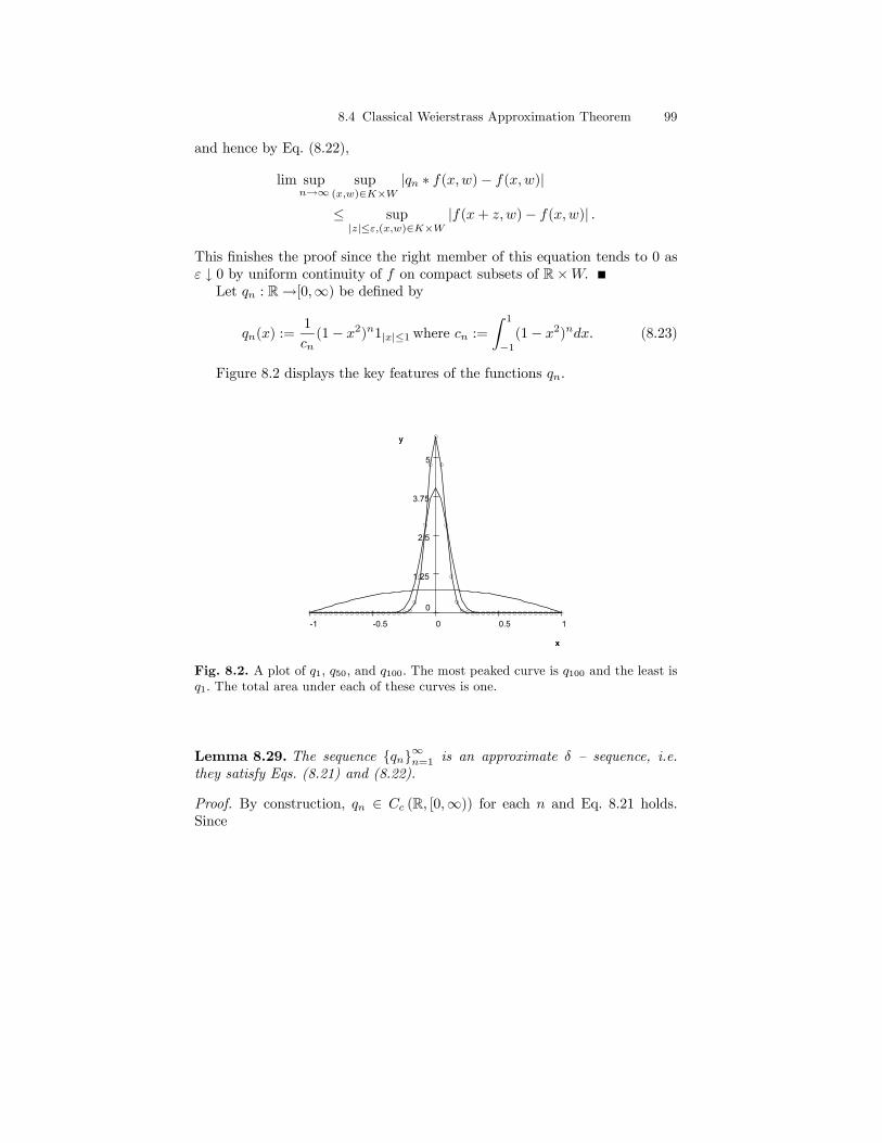
8.4 Classical Weierstrass Approximation Theorem 99
and hence by Eq. (8.22),
lim supn→∞
sup(x,w)∈K×W
|qn ∗ f(x,w)− f(x,w)|
≤ sup|z|≤ε,(x,w)∈K×W
|f(x+ z,w)− f(x,w)| .
This finishes the proof since the right member of this equation tends to 0 asε ↓ 0 by uniform continuity of f on compact subsets of R×W.Let qn : R→[0,∞) be defined by
qn(x) :=1
cn(1− x2)n1|x|≤1where cn :=
Z 1
−1(1− x2)ndx. (8.23)
Figure 8.2 displays the key features of the functions qn.
10.50-0.5-1
5
3.75
2.5
1.25
0
x
y
x
y
Fig. 8.2. A plot of q1, q50, and q100. The most peaked curve is q100 and the least isq1. The total area under each of these curves is one.
Lemma 8.29. The sequence {qn}∞n=1 is an approximate δ — sequence, i.e.they satisfy Eqs. (8.21) and (8.22).
Proof. By construction, qn ∈ Cc (R, [0,∞)) for each n and Eq. 8.21 holds.Since

100 8 The Riemann IntegralZ|x|≥ε
qn(x)dx =2R 1ε(1− x2)ndx
2R ε0(1− x2)ndx+ 2
R 1ε(1− x2)ndx
≤R 1ε
xε (1− x2)ndxR ε
0xε (1− x2)ndx
=(1− x2)n+1|1ε(1− x2)n+1|ε0
=(1− ε2)n+1
1− (1− ε2)n+1→ 0 as n→∞,
the proof is complete.
Notation 8.30 Let Z+ := N ∪ {0} and for x ∈ Rd and α ∈ Zd+ let xα =Qdi=1 x
αii and |α| =Pd
i=1 αi. A polynomial on Rd is a function p : Rd → C ofthe form
p(x) =X
α:|α|≤Npαx
α with pα ∈ C and N ∈ Z+.
If pα 6= 0 for some α such that |α| = N, then we define deg(p) := N to bethe degree of p. The function p has a natural extension to z ∈ Cd, namelyp(z) =
Pα:|α|≤N pαz
α where zα =Qd
i=1 zαii .
Theorem 8.31 (Weierstrass Approximation Theorem). Suppose thatK ⊂ Rd is a compact subset and f ∈ C(K,C)2 . Then there exists polynomialspn on Rd such that pn → f uniformly on K.
Proof. Choose λ > 0 and b ∈ Rd such thatK0 := λK − b := {λx− b : x ∈ K} ⊂ Bd
where Bd := (0, 1)d . The function F (y) := f¡λ−1 (y + b)
¢for y ∈ K0 is in
C (K0,C) and if pn (y) are polynomials on Rd such that pn → F uniformlyon K0 then pn (x) := pn (λx− b) are polynomials on Rd such that pn → funiformly on K. Hence we may now assume that K is a compact subset ofBd.Let g ∈ C (K ∪Bc
d) be defined by
g (x) =
½f (x) if x ∈ K0 if x ∈ Bc
d
and then use the Tietze extension Theorem 7.4 to find a continuous functionF ∈ C(Rd,C) such that F = g|K∪Bc
d. If pn are polynomials on Rd such
2 Note that f is automatically bounded because if not there would exist un ∈ Ksuch that limn→∞ |f (un)| = ∞. Using Theorem 8.2 we may, by passing to asubsequence if necessary, assume un → u ∈ K as n→∞ . Now the continuity off would then imply
∞ = limn→∞
|f (un)| = |f (u)|which is absurd since f takes values in C.

8.4 Classical Weierstrass Approximation Theorem 101
that pn → F uniformly on [0, 1]d then pn also converges to f uniformly onK. Hence, by replacing f by F, we may now assume that f ∈ C(Rd,C),K = Bd = [0, 1]
d , and f ≡ 0 on Bcd.
With qn defined as in Eq. (8.23), x ∈ [0, 1] and w ∈ Rd−1, let
fn(x,w) := (qn ∗ f)(x,w) =ZRqn(x− y)f(y, w)dy
=1
cn
Z[0,1]
f(y, w)£(1− (x− y)2)n1|x−y|≤1
¤dy
=1
cn
Z[0,1]
f(y, w)(1− (x− y)2)ndy =2nXk=0
Ank (w)x
k
where
Ank (w) =
Z[0,1]
f (y, w) ρnk (y) dy
and ρk is a polynomial function in y for each k. Then Ank (w) = 0 if w /∈
(0, 1)d−1 and using the uniform continuity of f on [0, 1]d , one easily showsAnk ∈ C
¡Rd−1,C
¢. Moreover by Lemmas 8.28 and 8.29, fn(x,w) → f(x,w)
uniformly for (x,w) ∈ [0, 1]d as n → ∞. This completes the proof of d = 1since then An
k are constants and pn (x) := fn (x) is a polynomial in x.The case of general d now follows by induction. Indeed, by the inductive
hypothesis there exists polynomial functions ank on Rd−1 such that
supw∈[0,1]d−1
|Ank (w)− ank (w)| ≤
1
2 (n+ 1)n.
Then
pn (x,w) :=2nXk=0
ank (w)xk
is a polynomial function on Rd such that
|f (x,w)− pn (x,w)| ≤ |f (x,w)− fn (x,w)|+ |fn (x,w)− pn (x,w)|
≤ εn +2nXk=0
|Ank (w)− ank (w)|xk
≤ εn +1
n
whereεn := sup
(x,w)∈[0,1]d|f (x,w)− fn (x,w)|→ 0 as n→∞.
This shows
sup(x,w)∈[0,1]d
|f (x,w)− pn (x,w)|→ 0 as n→∞
which completes the proof.

102 8 The Riemann Integral
Remark 8.32. The mapping (x, y) ∈ Rd × Rd → z = x + iy ∈ Cd is anisomorphism of vector spaces. Letting z = x − iy as usual, we have x = z+z
2and y = z−z
2i . Therefore under this identification any polynomial p(x, y) onRd ×Rd may be written as a polynomial q in (z, z), namely
q(z, z) = p(z + z
2,z − z
2i).
Conversely a polynomial q in (z, z) may be thought of as a polynomial p in(x, y), namely p(x, y) = q(x+ iy, x− iy).
Corollary 8.33 (ComplexWeierstrass Approximation Theorem). Sup-pose that K ⊂ Cd is a compact set and f ∈ C(K,C). Then there exists poly-nomials pn(z, z) for z ∈ Cd such that supz∈K |pn(z, z)− f(z)|→ 0 as n→∞.
Proof. This is an immediate consequence of Theorem 8.31 and Remark 8.32.
Example 8.34. Let K = S1 = {z ∈ C : |z| = 1} and A be the set of polynomi-als in (z, z) restricted to S1. Then A is dense in C(S1).3 Since z = z−1 on S1,we have shown polynomials in z and z−1 are dense in C(S1). This examplegeneralizes in an obvious way to K =
¡S1¢d ⊂ Cd.
Exercise 8.4. Suppose −∞ < a < b <∞ and f ∈ C ([a, b],C) satisfiesZ b
a
f (t) tndt = 0 for n = 0, 1, 2 . . . .
Show f ≡ 0.Exercise 8.5. Suppose f ∈ C (R,C) is a 2π — periodic function (i.e.f (x+ 2π) = f (x) for all x ∈ R) andZ 2π
0
f (x) einxdx = 0 for all n ∈ Z,
show again that f ≡ 0. Hint: Use Example 8.34 to shows that any 2π —periodic continuous function g on R is the uniform limit of trigonometricpolynomials of the form
p (x) =nX
k=−npke
ikx with pk ∈ C for all k.
3 Note that it is easy to extend f ∈ C(S1) to a function F ∈ C(C) by settingF (z) = zf( z
|z| ) for z 6= 0 and F (0) = 0. So this special case does not require theTietze extension theorem.

8.5 Iterated Integrals 103
8.5 Iterated Integrals
Theorem 8.35 (Baby Fubini Theorem). Let a, b, c, d ∈ R and f(s, t) ∈ Xbe a continuous function of (s, t) for s between a and b and t between c and d.Then the maps t→ R b
af(s, t)ds ∈ X and s→ R d
cf(s, t)dt are continuous andZ d
c
"Z b
a
f(s, t)ds
#dt =
Z b
a
"Z d
c
f(s, t)dt
#ds. (8.24)
Proof. See Exercise 8.7 for a sketch of another, more instructive, proof of thisresult. (BRUCE: Drop the following proof and leave it as an exercise.) Without loss of generality we may assume a < b and c < d. By uniform continuityof f (Theorem 8.2),
supc≤t≤d
kf(s, t)− f(s0, t)k→ 0 as s→ s0
and so by Lemma 8.7Z d
c
f(s, t)dt→Z d
c
f(s0, t)dt as s→ s0
showing the continuity of s → R dcf(s, t)dt. The other continuity assertion is
proved similarly.Now let
π = {a ≤ s0 < s1 < · · · < sm = b} and π0 = {c ≤ t0 < t1 < · · · < tn = d}
be partitions of [a, b] and [c, d] respectively. For s ∈ [a, b] let sπ = si if s ∈(si, si+1] and i ≥ 1 and sπ = s0 = a if s ∈ [s0, s1]. Define tπ0 for t ∈ [c, d]analogously. ThenZ b
a
"Z d
c
f(s, t)dt
#ds =
Z b
a
"Z d
c
f(s, tπ0)dt
#ds+
Z b
a
επ0(s)ds
=
Z b
a
"Z d
c
f(sπ, tπ0)dt
#ds+ δπ,π0 +
Z b
a
επ0(s)ds
where
επ0(s) =
Z d
c
f(s, t)dt−Z d
c
f(s, tπ0)dt
and
δπ,π0 =
Z b
a
"Z d
c
{f(s, tπ0)− f(sπ, tπ0)} dt#ds.
The uniform continuity of f and the estimates

104 8 The Riemann Integral
sups∈[a,b]
kεπ0(s)k ≤ sups∈[a,b]
Z d
c
kf(s, t)− f(s, tπ0)k dt
≤ (d− c) sup {kf(s, t)− f(s, tπ0)k : (s, t) ∈ Q}and
kδπ,π0k ≤Z b
a
"Z d
c
kf(s, tπ0)− f(sπ, tπ0)k dt#ds
≤ (b− a)(d− c) sup {kf(s, t)− f(s, tπ0)k : (s, t) ∈ Q}allow us to conclude thatZ b
a
"Z d
c
f(s, t)dt
#ds−
Z b
a
"Z d
c
f(sπ, tπ0)dt
#ds→ 0 as |π|+ |π0|→ 0.
By symmetry (or an analogous argument),Z d
c
"Z b
a
f(s, t)ds
#dt−
Z d
c
"Z b
a
f(sπ, tπ0)ds
#dt→ 0 as |π|+ |π0|→ 0.
This completes the proof sinceZ b
a
"Z d
c
f(sπ, tπ0)dt
#ds =
X0≤i<m,0≤j<n
f(si, tj)(si+1 − si)(tj+1 − tj)
=
Z d
c
"Z b
a
f(sπ, tπ0)ds
#dt.
Proposition 8.36 (Equality of Mixed Partial Derivatives). Let Q =(a, b) × (c, d) be an open rectangle in R2 and f ∈ C(Q,X). Assume that∂∂tf(s, t),
∂∂sf(s, t) and
∂∂t
∂∂sf(s, t) exists and are continuous for (s, t) ∈ Q,
then ∂∂s
∂∂tf(s, t) exists for (s, t) ∈ Q and
∂
∂s
∂
∂tf(s, t) =
∂
∂t
∂
∂sf(s, t) for (s, t) ∈ Q. (8.25)
Proof. Fix (s0, t0) ∈ Q. By two applications of Theorem 8.13,
f(s, t) = f(st0 , t) +
Z s
s0
∂
∂σf(σ, t)dσ
= f(s0, t) +
Z s
s0
∂
∂σf(σ, t0)dσ +
Z s
s0
dσ
Z t
t0
dτ∂
∂τ
∂
∂σf(σ, τ) (8.26)
and then by Fubini’s Theorem 8.35 we learn
f(s, t) = f(s0, t) +
Z s
s0
∂
∂σf(σ, t0)dσ +
Z t
t0
dτ
Z s
s0
dσ∂
∂τ
∂
∂σf(σ, τ).
Differentiating this equation in t and then in s (again using two more appli-cations of Theorem 8.13) shows Eq. (8.25) holds.
8.6 Exercises 105
8.6 Exercises
Throughout these problems, (X, k·k) is a Banach space.Exercise 8.6. Show f = (f1, . . . , fn) ∈ S([a, b],Rn) iff fi ∈ S([a, b],R) fori = 1, 2, . . . , n andZ b
a
f(t)dt =
ÃZ b
a
f1(t)dt, . . . ,
Z b
a
fn(t)dt
!.
Here Rn is to be equipped with the usual Euclidean norm. Hint: Use Lemma8.7 to prove the forward implication.
Exercise 8.7. Prove Theorem 8.35 using the following strategy.
1. Use the results from the proof in the text of Theorem 8.35 that
s→Z d
c
f(s, t)dt and t→Z b
a
f(s, t)ds
are continuous maps.2. For the moment take X = R and prove Eq. (8.24) holds by first proving itholds when f (s, t) = smtn withm,n ∈ N0. Then use this result along withTheorem 8.31 to show Eq. (8.24) holds for all f ∈ C ([a, b]× [c, d],R) .
3. For the general case, use the special case proved in item 2. along withHahn - Banach theorem.
Exercise 8.8. Give another proof of Proposition 8.36 which does not useFubini’s Theorem 8.35 as follows.
1. By a simple translation argument we may assume (0, 0) ∈ Q and we aretrying to prove Eq. (8.25) holds at (s, t) = (0, 0).
2. Let h(s, t) := ∂∂t
∂∂sf(s, t) and
G(s, t) :=
Z s
0
dσ
Z t
0
dτh(σ, τ)
so that Eq. (8.26) states
f(s, t) = f(0, t) +
Z s
0
∂
∂σf(σ, t0)dσ +G(s, t)
and differentiating this equation at t = 0 shows
∂
∂tf(s, 0) =
∂
∂tf(0, 0) +
∂
∂tG(s, 0). (8.27)
Now show using the definition of the derivative that

106 8 The Riemann Integral
∂
∂tG(s, 0) =
Z s
0
dσh(σ, 0). (8.28)
Hint: Consider
G(s, t)− t
Z s
0
dσh(σ, 0) =
Z s
0
dσ
Z t
0
dτ [h(σ, τ)− h(σ, 0)] .
3. Now differentiate Eq. (8.27) in s using Theorem 8.13 to finish the proof.
Exercise 8.9. Give another proof of Eq. (8.24) in Theorem 8.35 based onProposition 8.36. To do this let t0 ∈ (c, d) and s0 ∈ (a, b) and define
G(s, t) :=
Z t
t0
dτ
Z s
s0
dσf(σ, τ)
Show G satisfies the hypothesis of Proposition 8.36 which combined with twoapplications of the fundamental theorem of calculus implies
∂
∂t
∂
∂sG(s, t) =
∂
∂s
∂
∂tG(s, t) = f(s, t).
Use two more applications of the fundamental theorem of calculus along withthe observation that G = 0 if t = t0 or s = s0 to conclude
G(s, t) =
Z s
s0
dσ
Z t
t0
dτ∂
∂τ
∂
∂σG(σ, τ) =
Z s
s0
dσ
Z t
t0
dτ∂
∂τf(σ, τ). (8.29)
Finally let s = b and t = d in Eq. (8.29) and then let s0 ↓ a and t0 ↓ c toprove Eq. (8.24).
Exercise 8.10 (Product Rule). Prove items 1. and 2. of Lemma 8.9. Thiscan be modeled on the standard proof for real valued functions.
Exercise 8.11 (Chain Rule). Prove the chain rule in Proposition 8.10.Again this may be modeled on the on the standard proof for real valuedfunctions.
Exercise 8.12. To each A ∈ L (X) , we may define LA, RA : L (X)→ L (X)by
LAB = AB and RAB = BA for all B ∈ L (X) .
Show LA, RA ∈ L (L (X)) and that
kLAkL(L(X)) = kAkL(X) = kRAkL(L(X)) .
Exercise 8.13. Suppose that A : R → L(X) is a continuous function andU, V : R→ L(X) are the unique solution to the linear differential equations
V (t) = A(t)V (t) with V (0) = I (8.30)

8.6 Exercises 107
andU(t) = −U(t)A(t) with U(0) = I. (8.31)
Prove that V (t) is invertible and that V −1(t) = U(t)4 , where by abuse ofnotation I am writing V −1 (t) for [V (t)]−1 . Hints: 1) show d
dt [U(t)V (t)] = 0(which is sufficient if dim(X) < ∞) and 2) show compute y(t) := V (t)U(t)solves a linear differential ordinary differential equation that has y ≡ Id as anobvious solution. (The results of Exercise 8.12 may be useful here.) Then usethe uniqueness of solutions to linear ODEs.
Exercise 8.14. Suppose that (X, k·k) is a Banach space, J = (a, b) with−∞ ≤ a < b ≤ ∞ and fn : R → X are continuously differentiable functionssuch that there exists a summable sequence {an}∞n=1 satisfying
kfn (t)k+°°°fn (t)°°° ≤ an for all t ∈ J and n ∈ N.
Show:
1. supn°°°fn(t+h)−fn(t)h
°°° : (t, h) ∈ J ×R 3 t+ h ∈ J and h 6= 0o≤ an.
2. The function F : R→ X defined by
F (t) :=∞Xn=1
fn (t) for all t ∈ J
is differentiable and for t ∈ J,
F (t) =∞Xn=1
fn (t) .
Exercise 8.15. Suppose that A ∈ L(X). Show directly that:
1. etA define in Eq. (8.19) is convergent in L(X) when equipped with theoperator norm.
2. etA is differentiable in t and that ddte
tA = AetA.
Exercise 8.16. Suppose that A ∈ L(X) and v ∈ X is an eigenvector of Awith eigenvalue λ, i.e. that Av = λv. Show etAv = etλv. Also show that ifX = Rn and A is a diagonalizable n× n matrix with
A = SDS−1 with D = diag(λ1, . . . , λn)
then etA = SetDS−1 where etD = diag(etλ1 , . . . , etλn). Here diag(λ1, . . . , λn)denotes the diagonal matrix Λ such that Λii = λi for i = 1, 2, . . . , n.
Exercise 8.17. Suppose that A,B ∈ L(X) and [A,B] := AB − BA = 0.Show that e(A+B) = eAeB.
4 The fact that U(t) must be defined as in Eq. (8.31) follows from Lemma 8.9.
108 8 The Riemann Integral
Exercise 8.18. Suppose A ∈ C(R, L(X)) satisfies [A(t), A(s)] = 0 for alls, t ∈ R. Show
y(t) := e(R t0A(τ)dτ)x
is the unique solution to y(t) = A(t)y(t) with y(0) = x.
Exercise 8.19. Compute etA when
A =
µ0 1−1 0
¶and use the result to prove the formula
cos(s+ t) = cos s cos t− sin s sin t.Hint: Sum the series and use etAesA = e(t+s)A.
Exercise 8.20. Compute etA when
A =
0 a b0 0 c0 0 0
with a, b, c ∈ R. Use your result to compute et(λI+A) where λ ∈ R and I isthe 3× 3 identity matrix. Hint: Sum the series.
Exercise 8.21. Prove Theorem 8.24 using the following outline.
1. Using the right continuity at 0 and the semi-group property for Tt, showthere are constants M and C such that kTtkL(X) ≤MCt for all t > 0.
2. Show t ∈ [0,∞)→ Tt ∈ L(X) is continuous.3. For ε > 0, let Sε := 1
ε
R ε0Tτdτ ∈ L(X). Show Sε → I as ε ↓ 0 and
conclude from this that Sε is invertible when ε > 0 is sufficiently small.For the remainder of the proof fix such a small ε > 0.
4. Show
TtSε =1
ε
Z t+ε
t
Tτdτ
and conclude from this that
limt↓0
µTt − I
t
¶Sε =
1
ε(Tε − IdX) .
5. Using the fact that Sε is invertible, conclude A = limt↓0 t−1 (Tt − I) existsin L(X) and that
A =1
ε(Tε − I)S−1ε .
6. Now show, using the semigroup property and step 4., that ddtTt = ATt for
all t > 0.

8.6 Exercises 109
7. Using step 5, show ddte−tATt = 0 for all t > 0 and therefore e−tATt =
e−0AT0 = I.
Exercise 8.22 (Duhamel’ s Principle I). Suppose that A : R → L(X) isa continuous function and V : R→ L(X) is the unique solution to the lineardifferential equation in Eq. (8.30). Let x ∈ X and h ∈ C(R,X) be given. Showthat the unique solution to the differential equation:
y(t) = A(t)y(t) + h(t) with y(0) = x (8.32)
is given by
y(t) = V (t)x+ V (t)
Z t
0
V (τ)−1h(τ) dτ. (8.33)
Hint: compute ddt [V
−1(t)y(t)] (see Exercise 8.13) when y solves Eq. (8.32).
Exercise 8.23 (Duhamel’ s Principle II). Suppose that A : R→ L(X) isa continuous function and V : R→ L(X) is the unique solution to the lineardifferential equation in Eq. (8.30). Let W0 ∈ L(X) and H ∈ C(R, L(X)) begiven. Show that the unique solution to the differential equation:
W (t) = A(t)W (t) +H(t) with W (0) =W0 (8.34)
is given by
W (t) = V (t)W0 + V (t)
Z t
0
V (τ)−1H(τ) dτ. (8.35)
Exercise 8.24. Give another proof Corollary 8.14 based on Remark 8.12.Hint: the Hahn Banach theorem implies
kf(b)− f(a)k = supλ∈X∗, λ6=0
|λ(f(b))− λ(f(a))|kλk .


![Choudhary]_ Metric Spaces](https://img.pdfslide.us/doc/110x75/5695d2261a28ab9b02994972/choudhary-metric-spaces.jpg)